BDDC and FETI-DP for the Virtual Element Method

Abstract.

We build and analyze Balancing Domain Decomposition by Constraint (BDDC) and Finite Element Tearing and Interconnecting Dual Primal (FETI-DP) preconditioners for elliptic problems discretized by the virtual element method (VEM). We prove polylogarithmic condition number bounds, independent of the number of subdomains, the mesh size, and jumps in the diffusion coefficients. Numerical experiments confirm the theory.

1. Introduction

The ever-increasing interest in methods based on polygonal and polyhedral meshes for the numerical solution of PDEs stems from the high flexibility that polytopic grids allow in the treatment of complex geometries, which presently turns out to be, in many applications in computational engineering and scientific computing, as crucial a task as the construction and numerical solution of the discretized equations. Examples of methods where the discretization is based on arbitrarily shaped polytopic meshes include: Mimetic Finite Differences [14, 25], Discontinuous Galerkin-Finite Element Method (DG-FEM) [1, 26], Hybridizable and Hybrid High-Order Methods [29, 31], Weak Galerkin Method [60], BEM-based FEM [55] and Polygonal FEM [57]. Among such methods, the virtual element method (VEM) [5] is a quite recent discretization framework which can be viewed as an extension of the Finite Element Methods (FEM). The main idea of VEM is to consider local approximation spaces including polynomial functions, but to avoid the explicit construction and integration of the associated shape functions, whence the name virtual. An implicit knowledge of the local shape functions allows the evaluation of the operators and matrices needed in the method. Its implementation is described in [7] and the $p$ and $hp$ versions of the method are discussed and analyzed in [4, 12, 51]. Despite its recent introduction, VEM has already been applied and extended to study a wide variety of different model problems. Within the VEM literature we recall applications to: parabolic problems [59], Cahn-Hilliard, Stokes, Navier-Stokes and Helmoltz equations [2, 3, 15, 16, 54], linear and nonlinear elasticity problems [30, 6, 36], general elliptic problems in mixed form [8], fracture networks [18], Laplace-Beltrami equation [35].

To ensure that the Virtual Element Method can achieve its full potential, it is however necessary to deal with the efficient solution of the associated linear system of equations, and, in particular, to provide good preconditioners. By proposing suitable choices for the degrees of freedom, the first works in this direction aimed at dealing with the increase of condition number of the stiffness matrix resulting from the degradation of the quality of the geometry [12, 4, 50] and/or to the increase in the polynomial order of the method [19]. In this paper we rather focus on the increase in the condition number resulting from decreasing the mesh-size. In view of a possible parallel implementation of the method, we choose to consider a Domain Decomposition approach [58]. In particular, we focus on the two preconditioning techniques which are, nowadays, considered as the most efficient: Balancing Domain Decomposition by Constraint (BDDC) [32] and Dual-Primal Finite Element Tearing and Interconnecting (FETI-DP) [34]. These are non overlapping domain decomposition methods, aiming at preconditioning the Schur complement with respect to the unknowns on the skeleton of the subdomain partition. Acting on dual problems – the BDDC method defines a preconditioner for the Schur complement of the linear matrix stemming from discretized PDE, whereas FETI-DP reformulates the problem as a constrained optimization problem and solves it by iterating on the set of Lagrange multipliers representing the fluxes across the interface between the non overlapping subdomains – the two methods have been proven to be spectrally equivalent [24, 49, 48]. While both the BDDC and FETI-DP methods have been already extensively studied in the context of many different discretization methods – spectral elements [53, 44], mortar discretizations [38, 41, 40, 39], Discontinuous Galerkin methods [33, 28], NURBS discretizations in isogeometric analysis [13, 17] – to the best of our knowledge, these preconditioners have not yet been considered for VEM methods.

Here we prove that properties of scalability, quasi-optimality and independence on the discontinuities of the elliptic operator coefficients across subdomain interfaces still hold when dealing with VEM. More specifically, for both preconditioners, we show that the condition number of the preconditioned matrix is bounded by a constant times

$$(1+\log(Hk^{2}/h))^{2},$$

where $H$, $h$ and $k$ are the subdomain mesh-size, the fine mesh-size and the polynomial order respectively, see Corollary 4.3. In order to prove such a result we show that the validity of several inequalities (see, e.g. Lemma 4.1 in the following) is independent of the properties of the discretization within the subdomains and only relies on the properties of the trace of the discretization on the interface. This allows us to avoid handling discrete functions which are only implicitly defined.

The paper is organized as follows. The basic notation, functional setting and the description of the Virtual Element Method are given in Section 2. The dual-primal preconditioners are introduced and analyzed in Section 3, whereas their algebraic forms are presented in Section 5. Numerical experiments that validate the theory are presented in Section 6.

2. The virtual element method (VEM)

For $\hat{\Omega}$ (resp. $\hat{\Gamma}$) denoting any two-dimensional (resp. one-dimensional) domain with diameter (resp. length) $\hat{H}$, we introduce the usual (properly scaled) norms and semi-norms for the functional spaces that we will need to use in the following:

$$\|w\|_{L^{2}(\hat{\Omega})}^{2}=\hat{H}^{-2}\int_{\hat{\Omega}}|w(x)|^{2}\,dx,\qquad\|w\|_{L^{2}(\hat{\Gamma})}^{2}=\hat{H}^{-1}\int_{\hat{\Gamma}}|w(\tau)|^{2}\,d\tau,$$

$$|w|_{H^{1}(\hat{\Omega})}^{2}=\int_{\hat{\Omega}}|\nabla w(x)|^{2}\,dx,\qquad|w(\tau)|_{H^{1}(\hat{\Gamma})}^{2}=\hat{H}\int_{\Gamma}|w^{\prime}(\tau)|^{2}\,d\tau,$$

$$|w|^{2}_{H^{s}(\hat{\Gamma})}=\hat{H}^{2s-1}\int_{\hat{\Gamma}}\,d\sigma\int_{\hat{\Gamma}}\,d\tau\frac{|w(\sigma)-w(\tau)|^{2}}{|\sigma-\tau|^{2s+1}},\ 0<s<1,$$

$$\|w\|_{H^{1}(\hat{\Omega})}^{2}=\|w\|_{L^{2}(\hat{\Omega})}^{2}+|w|_{H^{1}(\hat{\Omega})}^{2},\quad\|w\|_{H^{s}(\hat{\Gamma})}^{2}=\|w\|_{L^{2}(\hat{\Gamma})}^{2}+|w|_{H^{s}(\hat{\Gamma})}^{2},\ 0<s\leq 1.$$

Let us start by recalling the definition and the main properties of the Virtual Element Method [5]. To fix the ideas we focus on the following elliptic model problem:

$$-\nabla\cdot(\rho\nabla u)=f\ \text{ in }\Omega,\qquad u=0\ \text{ on }\partial\Omega,$$

with $f\in L^{2}(\Omega)$, where $\Omega\subset\mathbb{R}^{2}$ is a polygonal domain. We assume that the coefficient $\rho$ is a scalar such that for almost all $x\in\Omega$, $\alpha\leq\rho(x)\leq M$ for two constants $M\geq\alpha>0$. The variational formulation of such an equation reads

(2.1) $$\left\{\begin{array}[]{l}\text{find $u\in V:=H^{1}_{0}(\Omega)$ such that}\\[2.84526pt] a(u,v)=(f,v)\ \forall v\in V\end{array}\right.$$

with

$$a(u,v)=\int_{\Omega}\rho(x)\nabla u(x)\cdot\nabla v(x)\,dx,\qquad(f,v)=\int_{\Omega}f(x)v(x)\,dx.$$

We consider a family $\{\mathcal{T}_{h}\}_{h}$ of tessellations of $\Omega$ into a finite number of simple polygons $K$, and we let $\mathcal{E}_{h}$ be the set of edges $e$ of $\mathcal{T}_{h}$. We make the following assumptions on the tessellation

Assumption 2.1.

There exists constants $\gamma_{0},\gamma_{1}>0$ such that for all tessellations $\mathcal{T}_{h}$:

1. each element $K\in\mathcal{T}_{h}$ is star-shaped with respect to a ball of radius $\geq\gamma_{0}h_{K}$, where $h_{K}$ is the diameter of $K$;

2. for each element $K$ in $\mathcal{T}_{h}$ the distance between any two vertices of $K$ is $\geq\gamma_{1}h_{K}$.

For simplicity, we also make the following assumption

Assumption 2.2.

The tessellation $\mathcal{T}_{h}$ is quasi-uniform, that is there exist positive constants $c_{0}$, $c_{1}$ such that for any two elements $K$ and $K^{\prime}$ in $\mathcal{T}_{h}$ we have $\alpha_{0}\leq h_{K}/h_{K^{\prime}}\leq\alpha_{1}$.

Assumption 2.3.

For all $K$ there exists a constant $\rho_{K}$ such that the coefficient $\rho$ verifies $\rho=\rho_{K}$ on $K$.

Remark 2.4.

Assumption 2.3 ensures that for the computable projection $\Pi^{\nabla}_{K}$ the splitting (2.3) holds. Remark, however, that the virtual element method can also be defined for the case of coefficients varying within the elements of the tessellation [10], and that the theoretical analysis developed here, which essentially relies on the bound (2.5), can be extended to such a case (see Section 4.0.1).

The Virtual Element discretization space is first defined element by element starting from the edges of the tessellation. More precisely, for each polygon $K\in\mathcal{T}_{h}$ we define the space $\mathbb{B}_{k}(\partial K)$ as

$$\mathbb{B}_{k}(\partial K)=\{v\in C^{0}(\partial K):v|_{e}\in\mathbb{P}_{k}\ \forall e\in\mathcal{E}^{K}\},$$

where $\mathbb{P}_{k}$ denotes the set of polynomials of degree less than or equal to $k$, and where $\mathcal{E}^{K}$ denotes the set of edges of the polygon $K$. It is not difficult to see that $\mathbb{B}_{k}(\partial K)$ is a linear space of dimension $kn^{K}$ where $n^{K}$ is the number of vertices of the polygon $K$. Letting

(2.2) $$V^{K,k}=\{v\in H^{1}(K):\ v|_{\partial K}\in\mathbb{B}_{k}(\partial K),\ \Delta v\in\mathbb{P}_{k-2}(K)\}$$

(with $\mathbb{P}_{-1}=\{0\}$), the discrete space $V_{h}$ is defined as

$$V_{h} =\{v\in V:w|_{K}\in V^{K,k}\ \forall K\in\mathcal{T}_{h}\}=$$

$$=\{v\in V:\forall K\in\mathcal{T}_{h}\ w|_{\partial K}\in\mathbb{B}_{k}(\partial K),\ \Delta v|_{K}\in\mathbb{P}_{k-2}(K)\}.$$

A function $v_{h}\in V_{h}$ is uniquely determined by the following degrees of freedom

• the values of $v_{h}$ at the vertices of the tessellation;

• for each edge $e$, the values of $v_{h}$ at the $k-1$ internal points of the $k+1$-points Gauss-Lobatto quadrature rule on $e$;

• for each element $K$, the moments up to order $k-2$ of $v_{h}$ in $K$.

The degrees of freedom are then naturally split as boundary degrees of freedom (the first two sets) and interior degrees of freedom. Boundary degrees of freedom are nodal, and we let $\Upsilon$ denote the corresponding set of nodes, which includes the vertices of the tessellation as well as the union over all edges of the $k-1$ internal nodes of the $k+1$-points Gauss-Lobatto quadrature rule.

Using a Galerkin approach, the Virtual Element Method stems from replacing the bilinear form $a$ (which, due to the implicit definition of the discrete space, is not directly computable on discrete functions in terms of the degrees of freedom) with a suitable approximate bilinear form. More precisely, setting, for each $K\in\mathcal{T}_{h}$

$$a^{K}(u,v)=\int_{K}\rho\nabla u\cdot\nabla v,$$

the key observation is that, given any $v\in V^{K,k}$ and any $p\in\mathbb{P}_{k}(K)$ we can compute $a^{K}(p,v)$ by using Green’s formula (recall that $\rho=\rho_{K}$ constant in $K$)

$$a^{K}(p,v)=-\rho_{K}\int_{K}v\Delta p+\rho_{K}\int_{\partial K}v\frac{\partial p}{\partial n}.$$

Since $v$ is a piecewise polynomial on $\partial K$, $p$ a polynomial of order $k$, and $\Delta p$ a polynomial of order $k-2$, the right hand side can be computed directly from the degrees of freedom of $v_{h}$. This allows to define the “element by element” computable projection operator $\Pi^{\nabla}_{K}:V^{K,k}\longrightarrow\mathbb{P}_{k}(K)$ as

$$a^{K}(\Pi^{\nabla}_{K}u,q)=a^{K}(u,q)\quad\forall q\in\mathbb{P}_{k}(K).$$

The last equation defines $\Pi^{\nabla}_{K}u$ only up to a constant; this is fixed by prescribing

$$\sum_{i=1}^{n}\Pi^{\nabla}_{K}u(V_{i})=\sum_{i=1}^{n}u(V_{i}),\quad V_{i}\text{ vertices of }K, \text{for }k=1,$$

$$\int_{K}\Pi^{\nabla}_{K}u=\int_{K}u, \text{for }k\geq 2.$$

Clearly we have

(2.3) $$a^{K}(u,v)=a^{K}(\Pi^{\nabla}_{K}u,\Pi^{\nabla}_{K}v)+a^{K}(u-\Pi^{\nabla}_{K}u,v-\Pi^{\nabla}_{K}v).$$

The virtual element method stems from replacing the second term of the sum on the right hand side (which cannot be computed exactly), with an “equivalent” term, where the bilinear for $a^{K}$ is substituted by a computable symmetric bilinear $S_{a}^{K}$, resulting in defining

$$a^{K}_{h}(u,v)=a^{K}(\Pi^{\nabla}_{K}u,\Pi^{\nabla}_{K}v)+S_{a}^{K}(u-\Pi^{\nabla}_{K}u,v-\Pi^{\nabla}_{K}v).$$

Different choices are possible for the bilinear form $S_{a}^{K}$ (see [11]), the essential requirement being that it satisfies

(2.4) $$c_{0}a^{K}(v,v)\leq S_{a}^{K}(v,v)\leq c_{1}a^{K}(v,v),\quad\forall v\in V^{K,k}\ \text{ with }\Pi^{\nabla}_{K}v=0,$$

for two positive constants $c_{0}$ and $c_{1}$, so that we have

(2.5) $$(1+c_{0})a^{K}(v,v)\leq a^{K}_{h}(v,v)\leq(1+c_{1})a^{K}(v,v),\quad\forall v\in V^{K,k}.$$

In the numerical tests performed in Section 6 we made the standard choice of defining $S_{a}^{K}$ in terms of the vectors of local degrees of freedom as the properly scaled euclidean scalar product.

Finally, we let $a_{h}:V_{h}\times V_{h}\to\mathbb{R}$ be defined by

$$a_{h}(u_{h},v_{h})=\sum_{K}a_{h}^{K}(u_{h},v_{h}),$$

and we consider the following discrete problems of the form

Problem 2.5.

Find $u_{h}\in V_{h}$ such that

$$a_{h}(u_{h},v_{h})=f_{h}(v_{h})\qquad\forall v_{h}\in V_{h}.$$

For the study of the convergence, stability and robustness properties of the method we refer to [5, 10].

3. Domain decomposition for the Virtual Element Method

We assume that the set $\mathcal{T}_{h}$ can be split as $\mathcal{T}_{h}=\cup_{\ell}\mathcal{T}_{h}^{\ell}$, in such a way that $\Omega$ may be written as the union of $L$ disjoint polygonal subdomains $\Omega^{\ell}$ with

(3.1) $${\Omega^{\ell}}=\cup_{K\in\mathcal{T}_{h}^{\ell}}K.$$

Assumption 3.1.

We make the following assumptions:

1. the decomposition is geometrically conforming, that is, for each $\ell,m$, $\partial\Omega^{\ell}\cap\partial\Omega^{m}$ is either a vertex or a whole edge of both $\Omega^{\ell}$ and $\Omega^{m}$;

2. there exists a positive constant $\gamma_{2}$ such that for each $\ell$ the distance between any two vertices of $\Omega^{\ell}$ is $\geq\gamma_{2}\ \text{diam}(\Omega^{\ell})$;

Assumption 3.2.

For all $\ell$, there exists a scalar $\rho_{\ell}>0$ such that $\rho|_{\Omega^{\ell}}\simeq\rho_{\ell}$.

We let $\Gamma=\cup\partial\Omega^{\ell}\setminus\partial\Omega$ denote the skeleton of the decomposition. For simplicity we assume that the decomposition is quasi uniform:

Assumption 3.3.

There exists constants $\beta_{0}$ and $\beta_{1}$ such that for any two subdomains $\Omega^{\ell}$ and $\Omega^{m}$ we have $\beta_{0}\leq\text{diam}(\Omega^{\ell})/\text{diam}(\Omega^{m})\leq\beta_{1}$.

Remark 3.4.

We would like to point out that Assumption 3.1 is actually also an assumption on the tessellation $\mathcal{T}_{h}$, satisfied, for instance, if $\mathcal{T}_{h}$ is built by first introducing the $\Omega^{\ell}$s and then refining them. The design and testing of FETI-DP and BDDC type preconditioners on more general tessellation will be the object of a future study.

We are interested here in explicitly studying the dependence of the estimates that we are going to prove on the number and size of the subdomains, the number and size of the elements of the tessellations, and on order $k$ of the virtual element method. To this end, in the following we will employ the notation $A\lesssim B$ (resp. $A\gtrsim B$) to say that the quantity $A$ is bounded from above (resp. from below) by $cB$, with a constant $c$ independent of $\rho$ and depending on the tessellation and on the decomposition only via the constants in Assumptions 2.1-3 and 3.1-3. The expression $A\simeq B$ will stand for $A\lesssim B\lesssim A$.

Observe that, in view of the quasi uniformity assumptions on the tessellation $\mathcal{T}_{h}$ and on its decomposition into subdomains, we can introduce global mesh size parameters $H$ and $h$ such that for all $\ell$ and for all $K$

$$h_{K}\simeq h,\qquad\text{diam}(\Omega^{\ell})\simeq H.$$

In the following it will be useful to define several sets of “pointers” for identifying specific sets of nodes and edges. To this end, recalling that

$$\Upsilon=\{y_{i},\ i=1,\cdots,N\}$$

denotes the set of nodes corresponding to boundary degrees of freedom, we let

$$\mathcal{Y}=\{i:\ y_{i}\in\Gamma\}$$

identify those nodes lying on the interface $\Gamma$ of the decomposition of $\Omega$ into subdomains. For each subdomain $\Omega^{\ell}$ we let $\mathcal{Y}^{\ell}\subset\mathcal{Y}$

$$\mathcal{Y}^{\ell}=\{i\in\mathcal{Y}:y_{i}\in\partial\Omega^{\ell}\}$$

identify the set of nodes on the boundary of $\Omega^{\ell}$. We let $\mathcal{X}$ and $\mathcal{X}^{\ell}$ identify, respectively, the set of cross-points and the set of vertices of the subdomain $\Omega^{\ell}$

$$\mathcal{X}=\{i\in\mathcal{Y}:y_{i}\text{ is a cross point}\},\qquad\mathcal{X}^{\ell}=\mathcal{X}\cap\mathcal{Y}^{\ell}.$$

Moreover, letting $\mathcal{E}_{H}$ denote the set of those macro-edges $E$ of the decomposition which are interior to $\Omega$, for each $E\in\mathcal{E}_{H}$ we let

$$\mathcal{Y}_{E}=\{i\in\mathcal{Y}:\ y_{i}\in\bar{E}\},\qquad\mathcal{X}_{E}=\{i\in\mathcal{X}:\ y_{i}\in\bar{E}\}$$

identify respectively the set of nodes and the set of cross points belonging to $E$. For each node $y_{i}$ we let $\mathcal{N}_{i}$ identify the set of the $n_{i}$ subdomains to whose boundary $y_{i}$ belongs

$$\mathcal{N}_{i}=\{\ell:y_{i}\in\partial\Omega^{\ell}\},\qquad n_{i}=\#(\mathcal{N}_{i}).$$

Remark that for all $i\in\mathcal{Y}\setminus\mathcal{X}$ we will have $n_{i}=2$.

The subdomain spaces $V_{h}^{\ell}$ and bilinear forms $a_{h}^{\ell}:V_{h}^{\ell}\times V_{h}^{\ell}\to\mathbb{R}$ are defined, as usual, as

$$V_{h}^{\ell}={V_{h}}|_{\Omega^{\ell}},\qquad a_{h}^{\ell}(u_{h},v_{h})=\sum_{K\in\mathcal{T}_{h}^{\ell}}a_{h}^{K}(u_{h},v_{h}),$$

and we easily see that solving Problem 2.5 is equivalent to finding $u_{h}=(u_{h}^{\ell})_{\ell}\in\prod V_{h}^{\ell}$ minimizing

$$J(u_{h})=\frac{1}{2}\sum_{\ell}a^{\ell}_{h}(u_{h}^{\ell},u_{h}^{\ell})-\int_{\Omega}fu_{h}$$

subject to a continuity constraint across the interface. In view of (2.5) we immediately obtain that for all $u,v\in V_{h}^{\ell}$

$$a_{h}^{\ell}(u,v)\lesssim|u|_{1,\Omega^{\ell}}|v|_{1,\Omega^{\ell}},\qquad a_{h}^{\ell}(u,u)\simeq|u|_{1,\Omega^{\ell}}^{2}.$$

The FETI-DP and BDDC preconditioners are constructed according to the same strategy used in the finite element case. More precisely we let

$$\mathring{V}_{h}=\prod\mathring{V}_{h}^{\ell},\quad\text{ with }\quad\mathring{V}_{h}^{\ell}=V_{h}^{\ell}\cap H^{1}_{0}(\Omega^{\ell}),$$

and

(3.2) $$W_{h}=\prod_{\ell}W_{h}^{\ell},\quad\text{ with }\quad W_{h}^{\ell}={V_{h}^{\ell}}|_{\partial\Omega^{\ell}}.$$

Moreover, let $\widehat{W}_{h}\subset W_{h}$ denote the subset of traces of functions which are continuous across $\Gamma$:

(3.3) $$\widehat{W}_{h}=\{w_{h}\in W_{h}:\forall i\in\mathcal{Y},\ell,m\in\mathcal{N}_{i}\Rightarrow w_{h}^{\ell}(y_{i})=w_{h}^{m}(y_{i})\}.$$

Analogously we let $\widetilde{W}_{h}$ denote the subset of $W_{h}$ of traces of functions which are continuous at cross-points:

(3.4) $$\widetilde{W}_{h}=\{w_{h}\in W_{h}:\forall i\in\mathcal{X},\ell,m\in\mathcal{N}_{i}\Rightarrow w_{h}^{\ell}(y_{i})=w_{h}^{m}(y_{i})\}.$$

On $W_{h}$ we define a norm and a seminorm:

$$\|w_{h}\|_{1/2,*}^{2}=\sum_{\ell}\|w_{h}^{\ell}\|_{H^{1/2}(\partial\Omega^{\ell})}^{2},\qquad|w_{h}|_{1/2,*}^{2}=\sum_{\ell}|w_{h}^{\ell}|_{H^{1/2}(\partial\Omega^{\ell})}^{2}.$$

Moreover, for each macroedge $E=\Gamma^{\ell}\cap\Gamma^{m}\in\mathcal{E}_{H}$, we let $W^{E}_{h}=W^{\ell}_{h}|_{E}=W^{m}_{h}|_{E}$. The space $W_{h}^{E}$ is the order $k$ one dimensional finite element space on the grid induced on $E$ by the tessellation $\mathcal{T}_{h}$, which, in view of Assumptions 2.2, is quasi uniform of mesh size $h$. In particular, it satisfies standard inverse and direct inequalities (recall that we are using scaled norms and seminorms): for all $r,s$ with $0<r\leq k+1$, $0\leq s<\min\{3/2,r\}$, $w\in H^{r}(E)$ implies

(3.5) $$\inf_{v_{h}\in W_{h}^{E}}\|w-v_{h}\|_{H^{s}(E)}\lesssim\left(\frac{h}{Hk}\right)^{r-s}|w|_{H^{r}(E)},$$

and for all $s,r$ with $0\leq s\leq r<3/2$, $w_{h}\in W_{h}^{E}$ implies

(3.6) $$\|w_{h}\|_{H^{r}(E)}\lesssim\left(\frac{h}{Hk^{2}}\right)^{s-r}\|w_{h}\|_{H^{s}(E)}.$$

As usual, we define a local discrete lifting operator $\mathcal{L}_{h}^{\ell}:W_{h}^{\ell}\to V_{h}^{\ell}$ as

(3.7) $$a^{\ell}_{h}(\mathcal{L}_{h}^{\ell}w_{h},v_{h})=0, \forall v_{h}\in\mathring{V}_{h}^{\ell},$$

(3.8) $$\mathcal{L}_{h}^{\ell}w_{h}=w_{h} \ \text{ on }\partial\Omega^{\ell}.$$

The following proposition holds

Proposition 3.5.

$\mathcal{L}_{h}^{\ell}$ is well defined, and it verifies

$$|\mathcal{L}_{h}^{\ell}w_{h}|_{1,\Omega^{\ell}}\simeq|w_{h}|_{1/2,\partial\Omega^{\ell}}.$$

Proof.

We start by remarking that there exists a linear operator $\Pi_{SZ}:H^{1}(\Omega^{\ell})\to V^{\ell}_{h}$ such that, for $v\in H^{1+s}$, $0\leq s\leq k$ one has

(3.9) $$\|v-\Pi_{SZ}v\|_{0,\Omega^{\ell}}+h|v-\Pi_{SZ}v|_{1,\Omega^{\ell}}\lesssim h^{s+1}|v|_{s+1,\Omega^{\ell}}.$$

Moreover $\Pi_{SZ}$ can be constructed in such a way that if $v|_{\partial\Omega^{\ell}}\in W_{h}^{\ell}$ one has $\Pi_{SZ}v=v$ on $\partial\Omega^{\ell}$. This is achieved by modifying the proof of Proposition 4.2 in [52] by replacing the Clément operator by a Scott-Zhang type operator, as constructed, for instance, in equation (4.8.6) in [23]. In view of this result it is not difficult to construct an operator $L_{h}^{\ell}:W_{h}^{\ell}\to V_{h}^{\ell}$ satisfying $L^{\ell}_{h}w_{h}|_{\partial\Omega^{\ell}}=w_{h}$ and

(3.10) $$|L^{\ell}_{h}w_{h}|_{H^{1}(\Omega^{\ell})}\leq|w_{h}|_{H^{1/2}(\partial\Omega^{\ell})}.$$

In fact, letting $w_{h}^{\mathcal{H}}\in H^{1}(\Omega^{m})$ denote the harmonic lifting of $w_{h}$, we can define

$$L_{h}^{\ell}w_{h}=\Pi_{SZ}(w_{h}^{\mathcal{H}}).$$

Equation (3.10) follows from the stability of the continuous harmonic lifting and of $\Pi_{SZ}$. We now observe that $\mathcal{L}_{h}^{\ell}w_{h}-L_{h}^{\ell}w_{h}\in\mathring{V}_{h}^{\ell}$ satisfies

$$a_{h}^{\ell}(\mathcal{L}_{h}^{\ell}w_{h}-L_{h}^{\ell}w_{h},v_{h})=-a_{h}^{\ell}(L_{h}^{\ell}w_{h},v_{h})\quad\forall v_{h}\in\mathring{V}^{\ell}_{h}.$$

We can then write

$$|\mathcal{L}_{h}^{\ell}w_{h}-L_{h}^{\ell}w_{h}|^{2}_{1,\Omega^{\ell}}\lesssim a^{\ell}_{h}(\mathcal{L}_{h}^{\ell}w_{h}-L_{h}^{\ell}w_{h},\mathcal{L}_{h}^{\ell}w_{h}-L_{h}^{\ell}w_{h})=-a_{h}^{\ell}(L_{h}^{\ell}w_{h},\mathcal{L}_{h}^{\ell}w_{h}-L_{h}^{\ell}w_{h})$$

$$\lesssim|L_{h}^{\ell}w_{h}|_{1,\Omega^{\ell}}|\mathcal{L}_{h}^{\ell}w_{h}-L_{h}^{\ell}w_{h}|_{1,\Omega^{\ell}},$$

yielding

$$|\mathcal{L}_{h}^{\ell}w_{h}-L_{h}^{\ell}w_{h}|_{1,\Omega^{\ell}}\lesssim|L_{h}^{\ell}w_{h}|_{1,\Omega}\lesssim|w_{h}|_{1/2,\Omega}.$$

By triangular inequality we then obtain

$$|\mathcal{L}_{h}^{\ell}w_{h}|_{1,\Omega^{\ell}}\lesssim|L_{h}^{\ell}w_{h}|_{1,\Omega^{\ell}}+|\mathcal{L}_{h}^{\ell}w_{h}-L_{h}^{\ell}w_{h}|_{1,\Omega^{\ell}}\lesssim|w_{h}|_{1/2,\partial\Omega^{\ell}}.$$

∎

For $w_{h}=(w_{h}^{\ell})_{\ell}\in W_{h}$ we let $\mathcal{L}_{h}(w_{h})=(\mathcal{L}_{h}^{\ell}w_{h}^{\ell})_{\ell}$, so that we can split $V_{h}$ as $\mathring{V}_{h}\oplus\mathcal{L}_{h}\widehat{W}_{h}$.

We can then define a bilinear for $s:W_{h}\times W_{h}\to\mathbb{R}$ as

$$s(w_{h},v_{h}):=\sum_{\ell}a^{\ell}_{h}(\mathcal{L}_{h}^{\ell}w_{h},\mathcal{L}_{h}^{\ell}v_{h}).$$

Problem 2.5 can be split as the combination of two independent problems

Problem 3.6.

Find $\mathring{u}_{h}\in\mathring{V}_{h}$ such that for all $v_{h}\in\mathring{V}_{h}$

$$a_{h}(\mathring{u}_{h},v_{h})=f_{h}(v_{h}).$$

Problem 3.7.

Find $w_{h}\in\widehat{W}_{h}$ such that for all $v_{h}\in\widehat{W}_{h}$

$$s(w_{h},v_{h})=\langle f,\mathcal{L}_{h}v_{h}\rangle.$$

The proof of the following proposition is trivial.

Proposition 3.8.

For all $v_{h},w_{h}\in W_{h}$ we have

(3.11) $$s(v_{h},w_{h})\lesssim|w_{h}|_{1/2,*}|v_{h}|_{1/2,*},\qquad s(w_{h},w_{h})\gtrsim|w_{h}|_{1/2,*}^{2}.$$

Following the approach of [24] we introduce the operators $\mathcal{\widehat{S}}:\widehat{W}_{h}\to\widehat{W}_{h}^{\prime}$ and $\mathcal{\widetilde{S}}:\widetilde{W}_{h}\to\widetilde{W}_{h}^{\prime}$ defined respectively as

(3.12) $$\langle\mathcal{\widehat{S}}w_{h},v_{h}\rangle=s(w_{h},v_{h})\ \forall v_{h}\in\widehat{W}_{h},\qquad\langle\mathcal{\widetilde{S}}w_{h},v_{h}\rangle=s(w_{h},v_{h})\ \forall v_{h}\in\widetilde{W}_{h},$$

and we let $\mathcal{R}:\widehat{W}_{h}\to\widetilde{W}_{h}$ denote the natural injection operator. We observe that

$$\mathcal{\widehat{S}}=\mathcal{R}^{T}\mathcal{\widetilde{S}}\mathcal{R}.$$

Problem 3.7 becomes

(3.13) $$\mathcal{\widehat{S}}u=f.$$

The BDDC Preconditioner

In order to build the BDDC preconditioner, we introduce, as in [58], the weighted counting functions $\delta_{\ell}$ which are associated with each $\partial\Omega^{\ell}$ and are defined for $\gamma\in[1/2,\infty)$ by a sum of contribution from $\Omega^{\ell}$ and its neighbors. For $i\in\mathcal{Y}^{\ell}$, we set

(3.14) $$\delta_{\ell}(y_{i})=\frac{\sum_{j\in\mathcal{N}_{i}}\rho_{j}^{\gamma}}{\rho_{\ell}^{\gamma}}.$$

As in [48, 46], we define a scalar product (i.e. a symmetric positive definite bilinear form) $d:W_{h}\times W_{h}\to\mathbb{R}$ defined as

(3.15) $$d(w_{h},v_{h})=\sum_{\ell}\sum_{i\in\mathcal{Y}^{\ell}}d^{\ell,i}v^{\ell}(y_{i})w^{\ell}(y_{i}),$$

where the scaling coefficients $d^{\ell,i}$ defined as

(3.16) $$d^{\ell,i}=(\delta_{\ell}(y_{i}))^{-1}=\frac{\rho_{\ell}^{\gamma}}{\sum_{j\in\mathcal{N}_{i}}\rho_{j}^{\gamma}}.$$

We next introduce the projection operator $\mathcal{E}_{D}:\widetilde{W}_{h}\to\widehat{W}_{h}$, orthogonal with respect to the scalar product $d$:

(3.17) $$d(\mathcal{E}_{D}w_{h},v_{h})=d(w_{h},v_{h}),\ \forall v_{h}\in\widehat{W}_{h}.$$

With this notation we can define the BDDC method, as the preconditioned conjugate gradient method applied to system (3.13); the BDDC preconditioner $\mathcal{M}_{BDDC}:\widehat{W}_{h}^{\prime}\to\widehat{W}_{h}$ takes the form

(3.18) $$\mathcal{M}_{BDDC}=\mathcal{E}_{D}\mathcal{\widetilde{S}}^{-1}\mathcal{E}_{D}^{T}.$$

The FETI-DP Preconditioner

Following [24], we introduce the quotient space $\Sigma_{h}=\widetilde{W}_{h}/\widehat{W}_{h}$. We let $\Lambda_{h}=\Sigma_{h}^{\prime}$ denote its dual and we let $\mathcal{B}:\widetilde{W}_{h}\to\Sigma_{h}=\Lambda_{h}^{\prime}$ be the quotient mapping, defined as

$$\mathcal{B}w_{h}=w_{h}+\widehat{W}_{h}.$$

Observe that two element $w_{h}$ and $v_{h}$ are representative of the same equivalence class in $\Sigma_{h}$ if and only if they have the same jump across the interface: for $E\in\mathcal{E}_{H}$ with $E=\Gamma^{m}\cap\Gamma^{\ell}$ $w_{h}^{m}-w_{h}^{\ell}=v_{h}^{m}-v_{h}^{\ell}$. We can then identify $\Sigma_{h}$ with the set of jumps of elements of $W_{h}$. The quotient map $\mathcal{B}$ is then the operator that maps an element of $W_{h}$ to its jump on the interface.

Clearly

$$\widehat{W}_{h}=\ker(\mathcal{B})=\{w_{h}\in\widetilde{W}_{h}:\ b(w_{h},\lambda)=0,\ \forall\lambda\in\Lambda_{h}\},$$

where $b:\widetilde{W}_{h}\times\Lambda_{h}\to\mathbb{R}$ is defined as $b(w_{h},\lambda_{h})=\langle\mathcal{B}(w_{h}),\lambda_{h}\rangle$. Problem 2.5 is then equivalent to the following saddle point problem: find $w_{h}\in\widetilde{W}_{h}$, $\lambda_{h}\in\Lambda_{h}$ solution to

$$\mathcal{\widetilde{S}}w_{h}-\mathcal{B}^{T}\lambda_{h}=\tilde{f},\qquad\mathcal{B}w_{h}=0,$$

where $\tilde{f}\in W_{h}^{\prime}$ is defined by

$$\langle\tilde{f},w_{h}\rangle=\int_{\Omega}f\mathcal{L}_{h}w_{h}=\sum_{\ell}\int_{\Omega^{\ell}}f\mathcal{L}_{h}^{\ell}w_{h}^{\ell}.$$

Eliminating $w_{h}$ we obtain a problem in the unknown $\lambda_{h}\in\Lambda_{h}$ of the form

(3.19) $$\mathcal{B}\mathcal{\widetilde{S}}^{-1}\mathcal{B}^{T}\lambda_{h}=-\mathcal{B}\mathcal{\widetilde{S}}^{-1}\tilde{f}.$$

The SPD operator $\mathcal{B}\mathcal{\widetilde{S}}^{-1}\mathcal{B}^{T}$ is the one that the FETI-DP preconditioner tackles. Letting $\mathcal{B}^{+}:\Sigma_{h}\to\widetilde{W}_{h}$ be any right inverse of $\mathcal{B}$ (for $\eta\in\Sigma_{h}$, $\mathcal{B}^{+}\eta$ is any element in $\widetilde{W}_{h}$ such that $\mathcal{B}\mathcal{B}^{+}\eta=w_{h}$), we set

$$\mathcal{B}^{T}_{D}=(\mathbf{1}_{\widetilde{W}_{h}}-\mathcal{E}_{D})\mathcal{B}^{+},$$

where $\mathbf{1}_{\widetilde{W}_{h}}$ denotes the identity operator in the space $\widetilde{W}_{h}$. Remark that the definition of $\mathcal{B}_{D}^{T}$ is independent of the actual choice of $\mathcal{B}^{+}$. Indeed for $v_{1}$ and $v_{2}$ such that $\mathcal{B}v_{1}=\mathcal{B}v_{2}$ we have $\mathcal{B}_{D}^{T}v_{1}-\mathcal{B}_{D}^{T}v_{2}=(v_{1}-v_{2})-\mathcal{E}_{D}(v_{1}-v_{2})=0$ where the last equality derives from the fact that since $\mathcal{B}v_{1}=\mathcal{B}v_{2}$, we have $v_{1}-v_{2}\in\widehat{W}_{h}$.

The preconditioner $\mathcal{M}_{FETI}:\Sigma_{h}\to\Lambda_{h}$ for (3.19) takes the form

(3.20) $$\mathcal{M}_{FETI}=\mathcal{B}_{D}\mathcal{\widetilde{S}}\mathcal{B}_{D}^{T}.$$

4. Analysis of the two preconditioners

Let us now provide bounds on the condition number of the preconditioned systems. We observe that the space $W_{h}$ coincides with the analogous space that we would get by applying the same procedure in the finite element case with a triangular or polyhedral mesh sharing with $\mathcal{T}_{h}$ the nodes on the interface. It is then reasonable to expect that by defining BDDC and FETI-DP preconditioners as in the finite element case we would obtain the same estimates on the dependence of the condition number on $H$, $h$ and $k$. A possible way of analyzing the method could be to introduce an auxiliary standard finite element mesh inducing the same trace spaces on $\Gamma$, and to prove that this can be done while satisfying the assumptions needed for the analysis of the preconditioners in the FEM case. This would allow to carry over the results for the FEM method to the VEM method. Here, however, we prefer to start from scratch and, in view of a future extension to the three dimensional case, providing a proof that will be mostly independent on the properties of the tessellation inside the subdomains. We start by remarking that, by construction, we are in the framework of [49], yielding the equivalence between the BDDC and the FETI-DP preconditioners. In particular we have the identity

$$\mathcal{B}_{D}^{T}\mathcal{B}+\mathcal{E}_{D}=\mathbf{1}_{\widetilde{W}_{h}}.$$

In fact, it is not difficult to see that for all $w_{h}\in\widetilde{W}_{h}$ we have that $(\mathbf{1}_{\widetilde{W}_{h}}-\mathcal{B}_{D}^{T}\mathcal{B})w_{h}\in\widehat{W}_{h}$ and that we have

$$d((\mathbf{1}_{\widetilde{W}_{h}}-\mathcal{B}_{D}^{T}\mathcal{B})w_{h},v_{h})=d(w_{h},v_{h})\quad\text{ for all }v_{h}\in\widehat{W}_{h}.$$

Then, letting

$$\omega_{FETI-DP}=\kappa(\mathcal{M}_{FETI}(\mathcal{B}\mathcal{\widetilde{S}}^{-1}\mathcal{B}^{T})),\qquad\omega_{BDDC}=\kappa(\mathcal{M}_{BDDC}\mathcal{\widehat{S}}),$$

denote the condition numbers of the operators $\mathcal{M}_{FETI}(\mathcal{B}\mathcal{\widetilde{S}}^{-1}\mathcal{B}^{T})$ and $\mathcal{M}_{BDDC}\mathcal{\widehat{S}}$, we have ([49])

(4.1) $$\omega_{BDDC}\lesssim\max_{w_{h}\in\widetilde{W}_{h}}\frac{s(\mathcal{E}_{D}w_{h},\mathcal{E}_{D}w_{h})}{s(w_{h},w_{h})},\qquad\omega_{FETI-DP}\lesssim\max_{w_{h}\in\widetilde{W}_{h}}\frac{s(\mathcal{B}_{D}^{T}\mathcal{B}w_{h},\mathcal{B}_{D}^{T}\mathcal{B}w_{h})}{s(w_{h},w_{h})},$$

and

(4.2) $$\omega_{BDDC}\simeq\omega_{FETI-DP}.$$

In order to have a bound on both condition numbers, we then only need to bound $s(\mathcal{E}_{D}w_{h},\mathcal{E}_{D}w_{h})$ in terms of $s(w_{h},w_{h})$.

We start by proving a technical Lemma. For $w_{h}\in W_{h}$ let us consider the splitting

(4.3) $$w_{h}=w_{H}+\mathring{w}_{h},$$

where $w_{H}^{\ell}(y_{i})=w^{\ell}_{h}(y_{i})$ for all $i\in\mathcal{X}^{\ell}$, and $w_{H}^{\ell}(y_{i})=0$ for all $i\in\mathcal{Y}^{\ell}\setminus\mathcal{X}^{\ell}$ ($w_{H}^{\ell}$ coincides with $w_{h}^{\ell}$ at the vertices of $\Omega^{\ell}$ and it is zero at all other nodes on $\partial\Omega^{\ell}$). We have the following Lemma ([56, 22]), for which we present a new proof that only relies on the properties of space $W_{h}$ and is independent of the properties of the tessellation in the interior of the subdomains $\Omega^{\ell}$.

Lemma 4.1.

For all $w_{h}\in W_{h}^{E}$, $E\in\mathcal{E}_{H}$, letting $\mathring{w}_{h}\in W_{h}^{E}$ be defined by $\mathring{w}_{h}(y_{i})=w_{h}(y_{i})$ for all $i\in\mathcal{Y}_{E}\setminus\mathcal{X}_{E}$, and $\mathring{w}_{h}(y_{i})=0$ for $i\in\mathcal{X}_{E}$, we have

$$\|\mathring{w}_{h}\|_{H^{1/2}_{00}(E)}\lesssim(1+\log(Hk^{2}/h))|w_{h}|_{H^{1/2}(E)}+\sqrt{1+\log(Hk^{2}/h)}\|w_{h}\|_{L^{\infty}(E)}.$$

Proof.

We start by proving the result for the lowest order VEM method ($k=1$). We let $\mathring{W}_{h}^{E}$ be defined as

$$\mathring{W}_{h}^{E}=\{w_{h}\in W_{h}^{E}:\ w_{h}(y_{i})=0\text{ for all }i\in\mathcal{X}_{E}\}.$$

Let $\pi_{h}:L^{2}(E)\to W_{h}^{E}$ and $\pi_{h}^{0}:L^{2}(E)\to\mathring{W}_{h}^{E}$ denote the $L^{2}$-projection onto respectively $W_{h}^{E}$ and $\mathring{W}_{h}^{E}$. Moreover, let $i_{h}^{0}:W_{h}^{E}\to\mathring{W}_{h}^{E}$ be defined by

$$i_{h}^{0}w_{h}(y_{i})=w_{h}(y_{i})\ \text{ for all }i\in\mathcal{Y}_{E}\setminus\mathcal{X}_{E}.$$

Remark that for $w_{h}\in W_{h}^{E}$ we have

$$\|i_{h}^{0}w_{h}\|_{L^{2}(E)}^{2}\lesssim h\sum_{i\in\mathcal{Y}_{E}\setminus\mathcal{X}_{E}}|w_{h}(y_{i})|^{2}\lesssim h\sum_{i\in\mathcal{Y}_{E}}|w_{h}(y_{i})|^{2}\lesssim\|w_{h}\|^{2}_{L^{2}(E)}.$$

Consider now the operator $\pi_{h}^{1}=i_{h}^{0}\circ\pi_{h}:L^{2}(E)\to\mathring{W}_{h}^{E}$. We easily see that $\pi_{h}^{1}$ is $L^{2}$ bounded: for all $w\in L^{2}(E)$,

$$\|\pi_{h}^{1}w\|_{L^{2}(E)}\lesssim\|\pi_{h}w\|_{L^{2}(E)}\lesssim\|w\|_{L^{2}(E)}.$$

On the other hand, observing that $i_{h}^{0}\circ\pi_{h}^{0}=\pi_{h}^{0}$, we have that, for $w\in H^{1}_{0}(E)$

$$\|w-\pi_{h}^{1}w\|_{L^{2}(E)} =\|w-\pi_{h}^{0}w+i_{h}^{0}\pi_{h}^{0}w-i_{h}^{0}\pi_{h}w\|_{L^{2}(E)}\lesssim$$

$$\lesssim\|w-\pi_{h}^{0}w\|_{L^{2}(E)}+\|\pi_{h}^{0}w-\pi_{h}w\|_{L^{2}(E)}.$$

By adding and subtracting $w$ in the second term on the right hand side we obtain, for $w\in H^{1}_{0}(E)$,

$$\|w-\pi_{h}^{1}w\|_{L^{2}(E)}\lesssim\|w-\pi_{h}^{0}w\|_{L^{2}(E)}+\|w-\pi_{h}w\|_{L^{2}(E)}\lesssim\frac{h}{H}|w|_{H^{1}(E)}.$$

This allows us to prove, by a standard argument, that $\pi_{h}^{1}$ is $H^{1}_{0}$-bounded. In fact, letting $\Pi_{h}^{1}:H^{1}_{0}(E)\to\mathring{W}_{h}^{E}$ denote the $H^{1}_{0}(E)$ projection onto $\mathring{W}_{h}^{E}$, defined as

$$\Pi_{h}^{1}(w)=\arg\min_{v_{h}\in\mathring{W}_{h}^{E}}\left(\frac{1}{2}|v_{h}|_{1,E}^{2}-\langle w,v_{h}\rangle\right),$$

we have

$$|\pi_{h}^{1}w| {}_{H^{1}(E)}\lesssim$$

$$\lesssim|w|_{H^{1}(E)}+\left(\frac{h}{H}\right)^{-1}\|\pi_{h}^{1}w-\Pi_{h}^{1}w\|_{L^{2}(E)}\lesssim$$

$$\lesssim|w|_{H^{1}(E)}+\left(\frac{h}{H}\right)^{-1}\|\pi_{h}^{1}w-w\|_{L^{2}(E)}+\left(\frac{h}{H}\right)^{-1}\|w-\Pi_{h}^{1}w\|_{L^{2}(E)}\lesssim$$

$$\lesssim|w|_{H^{1}(E)}+\left(\frac{h}{H}\right)^{-1}\left(\frac{h}{H}\right)|w|_{H^{1}(E)}+\left(\frac{h}{H}\right)^{-1}\left(\frac{h}{H}\right)|w|_{H^{1}(E)}\lesssim|w|_{H^{1}(E)}.$$

By space interpolation we then deduce that $\pi_{h}^{1}$ is uniformly $H^{s}_{0}(E)$ bounded for all $s\in[0,1]$, $s\not=1/2$, that is for all $w\in H^{s}_{0}(E)$ we have

$$\|\pi_{h}^{1}w\|_{H^{s}_{0}(E)}\lesssim\|w\|_{H^{s}_{0}(E)},$$

with a constant independent of $s$, whereas for $w\in H^{1/2}_{00}(E)$ we have

$$\|\pi_{h}^{1}w\|_{H^{1/2}_{00}(E)}\lesssim\|w\|_{H^{1/2}_{00}(E)}.$$

We now recall that for $0<s<1/2$, the space $H^{s}(E)$ is embedded in $H^{s}_{0}(E)$ and we have ([20])

$$\|w\|_{H^{s}_{0}(E)}\lesssim\frac{1}{1-2s}|w|_{H^{s}(E)}+\frac{1}{\sqrt{1-2s}}\|w\|_{L^{\infty}(E)}.$$

Then, for $\varepsilon\in]0,1/2[$ and $w_{h}\in W_{h}^{E}$ we have

$$\|\pi_{h}^{1}w_{h}\|_{H^{1/2}_{00}(E)} \lesssim\left(\frac{h}{H}\right)^{-\varepsilon}\|\pi_{h}^{1}w_{h}\|_{H^{1/2-\varepsilon}_{0}(E)}\lesssim\left(\frac{h}{H}\right)^{-\varepsilon}\|w_{h}\|_{H^{1/2-\varepsilon}_{0}(E)}\lesssim$$

$$\lesssim\frac{1}{\varepsilon}\left(\frac{h}{H}\right)^{-\varepsilon}|w_{h}|_{H^{1/2-\varepsilon}(E)}+\frac{1}{\sqrt{\varepsilon}}\left(\frac{h}{H}\right)^{-\varepsilon}\|w_{h}\|_{L^{\infty}(E)}$$

$$\lesssim(1+\log(H/h))|w_{h}|_{H^{1/2}(E)}+\sqrt{1+\log(H/h)}\|w_{h}\|_{L^{\infty}(E)},$$

where the last inequality is obtained by choosing $\varepsilon=1/|1+\log(H/h)|$ . Observing that for $w_{h}\in W_{h}^{E}$ we have

$$\mathring{w}_{h}^{\ell}|_{E}=i_{h}^{0}w_{h}|_{E}=\pi_{h}^{1}w_{h}|_{E},$$

we immediately get the thesis for $k=1$. For $k=2$ the result is proven analogously. In order to prove the result for $k\geq 3$, we proceed as in [58], Section 7.4.1. We let $w_{h}^{\star}$ and $\mathring{w}_{h}^{\star}$ denote the two functions which are piecewise linear on the grid with mesh size $\gtrsim h^{\star}=h/k^{2}$ induced on $E$ by the nodes $y_{i}$, $i\in\mathcal{Y}_{E}$, and interpolating respectively $w_{h}$ and $\mathring{w}_{h}$ at such nodes. We know (see [27]) that the following equivalences hold

$$\|w_{h}^{\star}\|_{0,E}\simeq\|w_{h}\|_{0,E},\text{ and }\ \|w_{h}^{\star}\|_{1,E}\simeq\|w_{h}\|_{1,E},$$

whence

$$|w_{h}^{\star}|_{H^{1/2}(E)}\simeq|w_{h}|_{H^{1/2}(E)}\text{ and }\ |\mathring{w}_{h}^{\star}|_{H^{1/2}_{00}(E)}\simeq|\mathring{w}_{h}^{\star}|_{H^{1/2}_{00}(E)}.$$

Then, applying the Lemma for $k=1$ and $\mathring{w}_{h}^{\star}$ and $w_{h}^{\star}$, we obtain

$$\|\mathring{w}_{h}\|_{H^{1/2}_{00}(E)} \lesssim\|\mathring{w}^{\star}_{h}\|_{H^{1/2}_{00}(E)}\lesssim$$

$$\lesssim(1+\log(H/h^{\star}))|w_{h}^{\star}|_{H^{1/2}(E)}+\sqrt{1+\log(H/h^{\star})}\|w_{h}^{\star}\|_{L^{\infty(E)}}$$

$$\lesssim(1+\log(Hk^{2}/h))|w_{h}|_{H^{1/2}(E)}+\sqrt{1+\log(Hk^{2}/h)}\|w_{h}\|_{L^{\infty(E)}}.$$

∎

We are now able to prove the following lemma.

Lemma 4.2.

For all $w_{h}\in\widetilde{W}_{h}$ we have

(4.4) $$s(\mathcal{E}_{D}w_{h},\mathcal{E}_{D}w_{h})\lesssim(1+\log(Hk^{2}/h))^{2}s(w_{h},w_{h}).$$

Proof.

We start by observing that $v_{h}=\mathcal{E}_{D}w_{h}$ is uniquely defined by its single values $v_{i}$ at the nodes $y_{i}$, $i\in\mathcal{Y}$. A straightforward computation yields, for $i\in\mathcal{Y}$:

(4.5) $$v_{i}=\theta^{-1}_{i}\sum_{k\in\mathcal{N}_{i}}\rho^{\gamma}_{k}w^{m}_{h}(y_{i}),\qquad\theta_{i}=\sum_{k\in\mathcal{N}_{i}}\rho_{k}^{\gamma}.$$

Using the splitting (4.3) for both $w_{h}$ and $v_{h}$ and observing that $v_{H}=w_{H}$, we have that

$$\sum_{\ell}|w_{h}-v_{h}|^{2}_{1/2,\Gamma_{\ell}}\lesssim\sum_{\ell}|\mathring{w}_{h}^{\ell}-\mathring{v}_{h}|^{2}_{1/2,\Gamma_{\ell}}.$$

We observe that, for a given macroedge $E=\partial\Omega^{\ell}\cap\partial\Omega^{m}$, we have

$$\mathring{v}_{h}{|_{E}}=(\rho_{\ell}^{\gamma}+\rho_{m}^{\gamma})^{-1}(\rho_{\ell}^{\gamma}{\mathring{w}_{h}^{\ell}}|_{E}+\rho_{m}^{\gamma}{\mathring{w}_{h}^{m}}|_{E}),$$

whence

$$(\mathring{w}_{h}^{\ell}-\mathring{v}_{h}){|_{E}}=(\rho_{\ell}^{\gamma}+\rho_{m}^{\gamma})^{-1}\rho_{m}^{\gamma}(\mathring{w}_{h}^{\ell}-\mathring{w}_{h}^{m}).$$

Then, recalling that

(4.6) $$\rho_{\ell}((\rho_{\ell}^{\gamma}+\rho_{m}^{\gamma})^{-1}\rho_{m}^{\gamma})^{2}\leq\min\{\rho_{\ell},\rho_{m}\}\leq\rho_{m},$$

we can write

$$\sum_{\ell}\rho_{\ell}|\mathring{w}_{h}^{\ell}-\mathring{v}_{h} |^{2}_{1/2,\Gamma^{\ell}}\lesssim\sum_{\ell}\sum_{E\in\mathcal{E}_{\ell}}\rho_{\ell}|\mathring{w}_{h}^{\ell}-\mathring{v}_{h}|_{H^{1/2}_{00}(E)}^{2}$$

$$\lesssim\sum_{\ell}\sum_{E=\partial\Omega^{\ell}\cap\partial\Omega^{m}\in\mathcal{E}_{\ell}}\rho_{\ell}(\rho_{\ell}^{\gamma}+\rho_{m}^{\gamma})^{-2}\rho_{m}^{2\gamma}|\mathring{w}_{h}^{\ell}-\mathring{w}_{h}^{m}|_{H^{1/2}_{00}(E)}^{2}$$

$$=\sum_{E=\partial\Omega^{\ell}\cap\partial\Omega^{m}\in\mathcal{E}}(\rho_{\ell}^{\gamma}+\rho_{m}^{\gamma})^{-2}(\rho_{\ell}\rho_{m}^{2\gamma}+\rho_{m}\rho_{\ell}^{2\gamma})|\mathring{w}_{h}^{\ell}-\mathring{w}_{h}^{m}|_{H^{1/2}_{00}(E)}^{2}$$

$$\lesssim\sum_{E=\partial\Omega^{\ell}\cap\partial\Omega^{m}\in\mathcal{E}}\min\{\rho_{\ell},\rho_{m}\}|\mathring{w}_{h}^{\ell}-\mathring{w}_{h}^{m}|_{H^{1/2}_{00}(E)}^{2}.$$

We now recall that we have the following bound for any $w_{h}\in W_{h}^{E}$ with $w_{h}(x)=0$ for some $x\in E$

(4.7) $$\|w_{h}\|_{L^{\infty}(E)}\lesssim\sqrt{(1+\log(Hk^{2}/h))}|w_{h}|_{H^{1/2}(E)}.$$

This bound was proven for $k=1$ in [21] as well as in [20], where a proof only relying on the properties of $W_{h}^{E}$ was provided. It is straightforward to adapt such a proof to cover the case $k>1$. Using Lemma 4.1, as well as (4.7) (which we can apply since $w_{h}^{\ell}-w_{h}^{m}$ vanishes at the extrema of $E$) we have

$$|\mathring{w}_{h}^{\ell}-\mathring{w}_{h}^{m}|_{H^{1/2}_{00}(E)}^{2} \lesssim(1+\log(Hk^{2}/h))^{2}|w_{h}^{\ell}-w_{h}^{m}|^{2}_{H^{1/2}(E)}+$$

$$+(1+\log(Hk^{2}/h))\|w_{h}^{\ell}-w_{h}^{m}\|^{2}_{L^{\infty}(E)}\lesssim$$

$$\lesssim(1+\log(Hk^{2}/h))^{2}|w_{h}^{\ell}-w_{h}^{m}|^{2}_{H^{1/2}(E)}\lesssim$$

$$\lesssim(1+\log(Hk^{2}/h))^{2}(|w_{h}^{\ell}|_{H^{1/2}(E)}^{2}+|w_{h}^{m}|_{H^{1/2}(E)}^{2}),$$

whence we easily obtain

$$\sum_{\ell}\rho_{\ell}|\mathring{w}_{h}^{\ell}-\mathring{v}_{h}|^{2}_{1/2,\Gamma^{\ell}} \lesssim(1+\log(Hk^{2}/h))^{2}\sum_{\ell}\rho_{\ell}|w_{h}^{\ell}|_{H^{1/2}(\Gamma_{\ell})}\lesssim$$

$$\lesssim(1+\log(Hk^{2}/h))^{2}s(w_{h},w_{h}).$$

∎

In view of (4.1) and (4.2) we have the following corollary

Corollary 4.3.

The following bound on the condition numbers for BDDC and FETI-DP holds

$$\omega_{BDDC}\lesssim(1+\log(Hk^{2}/h))^{2},\qquad\omega_{FETI-DP}\lesssim(1+\log(Hk^{2}/h))^{2}.$$

4.0.1. Extension to other $H^{1}$ conforming VEM classes

While for simplicity we considered in our analysis the simpler early version of the VEM method, where the local space is defined by (2.2), it is not difficult to realize that the analysis presented here carries over to other $H^{1}$ conforming versions of the method. In particular, several VEM methods make use of an auxiliary enlarged local space $V_{aux}^{K,k}$ defined as

$$V_{aux}^{K,k}=\{v\in H^{1}(K):\ v|_{\partial K}\in\mathbb{B}_{k}(\partial K),\ \Delta v\in\mathbb{P}_{k}(K)\},$$

and define the local space $V^{K,k}$ as the subspace obtained by requiring that a certain number of degrees of freedom, corresponding to high order moments, are a function of the remaining ones. This is the case of the VEM space used for treating problems with coefficients that vary within each element [10], and of the nodal serendipity VEM [9]. As also for these new spaces it holds that $V_{aux}^{K,k}|_{\partial K}=\mathbb{B}_{k}(\partial K)$, it is not difficult to realize that our analysis carries over to such cases, provided we can verify that property (2.5) and Proposition 3.5 hold. These are indeed the only steps in our analysis which depend on the definition of $V^{K,k}$ within the elements. Observe that property (2.5) is one of the basic requirements in the construction of the VEM stabilized operator (see, e.g. (5.4) and (5.23) in [10]). As far as Proposition 3.5, its proof relies on the existence of a Scott-Zhang type operator satisfying an estimate of the form (3.9). The construction of such an operator, as proposed in [52] for the case here considered, carries over to other $H^{1}$ conforming VEM spaces, yielding (3.9) with constants possibly depending on $k$. It is in fact not difficult to verify that adapting such a construction to different definitions of the local space $V^{K,k}$ yields an operator that locally preserves polynomials of order $k$ (provided of course that they are contained in the local space).

Remark 4.4.

As far as the possible extension to other PDEs or to non $H^{1}$ conforming methods such as $H(div)$ conforming or discontinuous Galerkin, the same issues arise in the virtual element framework as in the finite element case, and, in view of the analysis performed here, we believe that the same solution strategies apply, tough the treatment of such cases is not immediate and needs further work.

5. Realizing the preconditioner

As already observed, both the FETI-DP and the BDDC preconditioner for the virtual element method are the same as for the finite element method, and a vast literature exists on how such methods are efficiently implemented, that carries over, essentially as it is, to our case. Nevertheless, for the sake of those reader with little experience in domain decomposition, we recall some details of the implementation, which we adapt to the notation used in the previous sections.

5.1. Functions

Functions in the different spaces are represented algebraically as follows.

• functions $u^{\ell}_{h}\in W_{h}^{\ell}$ are represented by the vectors $\mathbf{u}^{\ell}\in\mathbb{R}^{N_{\ell}}$ (with ${N_{\ell}}=\#(\mathcal{Y}^{\ell})$) of their values at the nodes $y_{i},i\in\mathcal{Y}^{\ell}$;

• functions $u_{h}=(u_{h}^{\ell})_{\ell}\in W_{h}$ will be represented by the vectors obtained by concatenating the $\mathbf{u}^{\ell}$s: $\mathbf{u}=(\mathbf{u}^{1},\cdots,\mathbf{u}^{\ell})\in\mathbb{R}^{N}$, $N=\sum_{\ell}{N_{\ell}}$;

• functions $\hat{u}_{h}\in\widehat{W}_{h}$ will be represented by the vectors $\hat{\mathbf{u}}\in\mathbb{R}^{\widehat{N}}$ ($\widehat{N}=\#(\mathcal{Y})$) of their values at the nodes on $\Gamma$;

• functions $\tilde{u}_{h}\in\widetilde{W}_{h}$ will be represented by the vectors $\tilde{\mathbf{u}}\in\mathbb{R}^{\widetilde{N}}$, of their single values at the crosspoints plus their double value at each of the nodes $y_{i}\in\mathcal{Y}\setminus\mathcal{X}$;

• the elements of $\Sigma_{h}$ (i.e. the jumps of functions in $\widetilde{W}_{h}$) will be represented by vectors $\mathbf{s}\in\mathbb{R}^{M}$, $M=\#(\mathcal{Y}\setminus\mathcal{X})$, of jump values at the nodes $y_{i}$, $i\in\mathcal{Y}\setminus\mathcal{X}$.

Corresponding to the splitting (4.3), the vectors $\widetilde{\mathbf{u}}\in\mathbb{R}^{\widetilde{N}}$ are split as

(5.1) $$\widetilde{\mathbf{u}}=[\mathbf{u}_{\Delta},\mathbf{u}_{\Pi}],$$

with $\mathbf{u}_{\Pi}\in\mathbb{R}^{{N_{\Pi}}}$ being the vector of values at the cross points (primal nodes), $u_{\Delta}^{\ell}$ being the vector of values of $u_{h}^{\ell}$ at the points $y_{i}$, $i\in\mathcal{Y}^{\ell}\setminus\mathcal{X}^{\ell}$ (dual nodes) and $\mathbf{u}_{\Delta}=(u_{\Delta}^{1},\cdots,u_{\Delta}^{L})\in\mathbb{R}^{{N_{\Delta}}}$ . Observe that, with the choices made in Section 3, we have ${N_{\Delta}}=2\#(\mathcal{Y}\setminus\mathcal{X})$, ${N_{\Pi}}=\#(\mathcal{X})$, and $N={N_{\Delta}}+\sum_{i\in\mathcal{X}}n_{i}$.

5.2. Operators

In order to implement the BDDC and the FETI-DP methods, we need to construct (or implement the action of) matrices corresponding to the different operators introduced in Section 3, and, in particular, to $\mathcal{E}_{D}$ and $\mathcal{B}^{T}_{D}$ and $\mathcal{\widetilde{S}}^{-1}$.

We start by letting $S_{\ell}\in\mathbb{R}^{{N_{\ell}}\times{N_{\ell}}}$ denote the ${N_{\ell}}\times{N_{\ell}}$ matrix realizing the operator $\mathcal{S}^{\ell}$, and we let $S\in\mathbb{R}^{N\times N}$, defined by

$$S=\left(\begin{array}[]{ccc}S_{1}&&\\ &\ddots&\\ &&S_{L}\end{array}\right),$$

be the block diagonal matrix realizing the operator $\mathcal{S}$. Observe that the matrix $S_{\ell}$ is the Schur complement, taken with respect to the degrees of freedom on $\partial\Omega^{\ell}$, of the stiffness matrix $A_{\ell}$ discretizing the bilinear form $a_{h}^{\ell}$ on the space $V_{h}^{\ell}$ defined in (3). Applying $S^{\ell}$ implies then solving by the VEM method a local version of problem (2.1) with non homogeneous boundary condition.

We let $\widehat{R}\in\mathbb{R}^{N\times\widehat{N}}$ and $\widetilde{R}\in\mathbb{R}^{N\times\widetilde{N}}$ denote the two matrices realizing the natural injection of $\widehat{W}_{h}$ and $\widetilde{W}_{h}$ into $W_{h}$, respectively, and let $R$ denote the matrix realizing the injection of $\widehat{W}_{h}$ into $\widetilde{W}_{h}$. These are matrices with $0$ and $1$ entries, whose action essentially consists in copying the value of the degrees of freedom in the right positions. With this notation, the matrices $\widetilde{S}\in\mathbb{R}^{\widetilde{N}\times\widetilde{N}}$ and $\widehat{S}\in\mathbb{R}^{\widehat{N}\times\widehat{N}}$, realizing the operators $\mathcal{\widetilde{S}}$ and $\mathcal{\widehat{S}}$, respectively, take the form

$$\widetilde{S}=\widetilde{R}^{T}S\widetilde{R},\qquad\widehat{S}=\widehat{R}^{T}S\widehat{R},$$

and we have

$$\widehat{S}=R^{T}\widetilde{S}R.$$

We let $D_{\ell}\in\mathbb{R}^{{N_{\ell}}\times{N_{\ell}}}$ be the diagonal matrix whose diagonal entry on the line corresponding to the node $y_{i},i\in\mathcal{Y}^{\ell}$ is equal to the scaling coefficient $d^{\ell,i}=\rho_{\ell}^{\gamma}/\sum_{j\in\mathcal{N}_{i}}\rho_{j}^{\gamma}$, and we assemble $D\in\mathbb{R}^{N\times N}$ as

$$D=\left(\begin{array}[]{ccc}D_{1}&&\\ &\ddots&\\ &&D_{L}\end{array}\right),$$

so that the scalar product $d:W_{h}\times W_{h}\in\mathbb{R}$ defined by (3.15) is realized by the matrix $D$. We easily check that we have $\widehat{R}^{T}D\widehat{R}=I_{\widehat{N}}$ (where $I_{\widehat{N}}$ denotes the $\widehat{N}\times\widehat{N}$ identity matrix). It is not difficult to verify that the matrix $E_{D}\in\mathbb{R}^{\widehat{N}\times\widetilde{N}}$ realizing the projector $\mathcal{E}_{D}$ is

$$E_{D}=\widehat{R}^{T}D\widetilde{R}\in\mathbb{R}^{\widehat{N}\times\widetilde{N}}.$$

In fact, letting $\widehat{\mathbf{w}}$ denote the vector of coefficients of $\mathcal{E}_{D}\widetilde{u}_{h}$, we have

$$\widehat{\mathbf{v}}^{T}\widehat{\mathbf{w}}=\widehat{\mathbf{v}}^{T}\,\widehat{R}^{T}D\widehat{R}\,\widehat{\mathbf{w}}=\widehat{\mathbf{v}}^{T}\,\widehat{R}^{T}D\widetilde{R}\,\tilde{\mathbf{u}},\qquad\text{ for all }\widehat{\mathbf{v}}\in\mathbb{R}^{\widehat{N}}.$$

Let us now come to the construction of the matrices corresponding to the jump operator $\mathcal{B}$ and its pseudo inverse $\mathcal{B}_{D}^{T}$. We let $B=[B_{1},\dots,B_{L}]\in\mathbb{R}^{M\times\widetilde{N}}$ denote the matrix with entries in the set $\{-1,0,1\}$, representing the jump operator. Observe that we have $BB^{T}=2I_{M}$, that is, in our case, $B^{T}/2$ is a right inverse of $B$, and this gives us the operator $\mathcal{B}^{+}$. Then $B^{T}_{D}\in\mathbb{R}^{\widetilde{N}\times M}$ can be defined as

$$B^{T}_{D}=(I_{\widetilde{N}}-RE_{D})B^{T}/2.$$

By direct computation it is not difficult to verify that ${B_{D}}$ is a scaled version of B

$${B_{D}}=[D^{\flat}_{1}B_{1},\dots,D^{\flat}_{L}B_{L}]$$

where $D^{\flat}_{\ell},l=1,\dots,L$, are diagonal scaling matrices with entries related to the neighboring subdomain of $\Omega_{\ell}$. More precisely, each row of $B_{\ell}$ with a non zero entry corresponds to a node $y_{i}$, $i\in\mathcal{Y}^{\ell}\setminus\mathcal{X}^{\ell}$, which verifies $y_{i}\in\partial\Omega_{\ell}\cap\partial\Omega_{k}$ for a unique $k$. The diagonal entry of $D^{\flat}_{\ell}$ corresponding to such node takes the value $d^{k,i}=\rho_{k}^{\gamma}/\sum_{j\in\mathcal{N}_{i}}\rho_{j}^{\gamma}$.

Then the system we deal with the BDDC method is

(5.2) $$\widehat{S}\hat{\mathbf{u}}=\hat{\mathbf{f}},$$

preconditioned with

(5.3) $$M_{BDDC}=E_{D}{\widetilde{S}}^{-1}E_{D}^{T},$$

matrix counterpart of (3.13) and (3.18) respectively.

The last matrix whose action we need to evaluate is ${\widetilde{S}}^{-1}$, corresponding to the inverse of the operator $\mathcal{\widetilde{S}}$. Different approaches have been proposed for its efficient implementation [42, 43, 45]. We start by observing that, corresponding to the splitting (5.1), the matrix ${\widetilde{S}}$ can be rewritten as

$$\widetilde{S}=\left(\begin{array}[]{cc}\widetilde{S}_{{\Delta\Delta}}&\widetilde{S}_{{\Delta\Pi}}\\ \widetilde{S}_{\Pi\Delta}&\widetilde{S}_{{\Pi\Pi}}\end{array}\right).$$

The matrix $\widetilde{S}_{\Delta\Delta}$ is block diagonal and invertible. Following [47], we can use block Cholesky elimination to get

(5.4) $${\widetilde{S}}^{-1}=\left(\begin{array}[]{cc}\widetilde{S}_{{\Delta\Delta}}^{-1}&0\\ 0&0\end{array}\right)+\left(\begin{array}[]{c}-\widetilde{S}_{{\Delta\Delta}}^{-1}\widetilde{S}_{{\Delta\Pi}}\\ I_{N_{\Pi}}\end{array}\right)\left(\widetilde{S}_{{\Pi\Pi}}-\widetilde{S}_{\Pi\Delta}\widetilde{S}^{-1}_{{\Delta\Delta}}\widetilde{S}_{{\Delta\Pi}}\right)^{-1}\left(\begin{array}[]{cc}-\widetilde{S}_{\Pi\Delta}\widetilde{S}^{-1}_{{\Delta\Delta}}&I_{N_{\Pi}}\end{array}\right)$$

Only the matrix $\tilde{S}_{{\Pi\Pi}}-\tilde{S}_{\Pi\Delta}\tilde{S}^{-1}_{{\Delta\Delta}}\tilde{S}_{{\Delta\Pi}}$ is assembled once for all (this is done by computing its action on the columns of $I_{N_{\Pi}}$). As far as the other matrices on the right hand side of the expression are concerned, only their action on a given vector needs to be implemented.

Each block $S_{{\Delta\Delta}}^{\ell}$ is the Schur complement with respect to the degrees of freedom interior to the subdomain $\Omega_{\ell}$ of the matrix $A_{0}^{\ell}$ obtained from the local stiffness matrix $A^{\ell}$ by eliminating the rows and columns corresponding to degrees of freedom attached to the cross points. In order to apply $\tilde{S}_{{\Delta\Delta}}^{-1}$ to a vector $\mathbf{r}$ one can then solve a system with the diagonal matrix

$$A_{0}=\left(\begin{array}[]{ccc}A^{1}_{0}&&\\ &\ddots&\\ &&A^{L}_{0}\end{array}\right).$$

More precisely,

$${\widetilde{S}}_{{\Delta\Delta}}^{-1}=C^{T}{A_{0}}^{-1}C,$$

where $C\in\mathbb{R}^{N_{dof}\times\widetilde{N}}$ (where $N_{dof}$ is the total number of degrees of freedom)is a matrix with $0$ and $1$ entries, defined in such a way that $\mathbf{z}=C\mathbf{r}$ is obtained by “copying” each entry of the vector $\mathbf{r}$ (which corresponds to a node $y_{i}$, $i\in\mathcal{Y}\setminus\mathcal{X}$ and to a subdomain $\ell$ with $y_{i}\in\mathcal{Y}^{\ell}$) in the line of $\mathbf{z}$ corresponding to the same node and subdomain.

Then the for the FETI-DP method, the matrix counterpart of (3.19) and (3.20), are

(5.5) $$B{\widetilde{S}}^{-1}B^{T}\lambda={\mathbf{g}},\qquad\qquad M_{FETI}=B_{D}{\widetilde{S}}B_{D}^{T},$$

with ${\mathbf{g}}$ proper right-hand side.

6. Numerical results.

In this section we present numerical results for the model elliptic problem

$$-\nabla\cdot(\rho\nabla u)=f\ \text{ in }\Omega=]0,1[^{2},\qquad u=0\ \text{ on }\partial\Omega.$$

We consider both a constant coefficient problem with $\rho=1$ and several problems with highly varying coefficients, with jumps across the interface. The domain $\Omega$ is decomposed into $N^{2}$ square subdomains as shown in Figure 1. Two types of discretizations are considered: a structured discretization with hexagonal elements and a Voronoi discretization (Figure 1, 2).

The interface problem (5.5) is solved by a preconditioned conjugate gradient method (PCG) with zero initial guess and relative tolerance of $10^{-6}$. The condition numbers are numerical approximations computed from the standard tridiagonal Lanczos matrix generated during the PCG iteration as the ratio between the maximum and the minimum eigenvalues, see e.g. [37]. All the numerical tests are performed in matlab R2014b^©.

6.1. The constant coefficient case

We start by testing the scalability and optimality of the methods on the simplest case of constant $\rho=1$. The right hand side is chosen as $f=\sin(\pi x)\sin(\pi y)$. Inside each subdomain, we consider virtual elements of order $k=1$. In Tables 1 and 3 (referring resp. to hexagonal and Voronoi meshes) we report the iteration counts and condition numbers of the FETI-DP preconditioned system (5.5) for increasing $N$ (number of subdomains in each coordinate direction) and $n$ (number of elements in each subdomain). The same quantities for the BDDC preconditioned system (5.2)-(5.3) on hexagonal meshes are reported in Table 2. In all three tests the largest problem ($N=64$, $n=70\times 80$) could not be tested due to memory limitations. The results are in agreement with the theoretical bound on the condition numbers (see Corollary (4.3)), moreover, comparing Tables 1 and 2, it clearly appears that the two spectra are almost identical. The small differences can be attributed to the different systems being solved: the Schur complement system (5.2)-(5.3) for BDDC and the Lagrange multipliers system (5.5) for FETI-DP; the different convergence histories for the two systems lead in some cases to slightly different iteration counts and Lanczos approximations of the extreme eigenvalues.

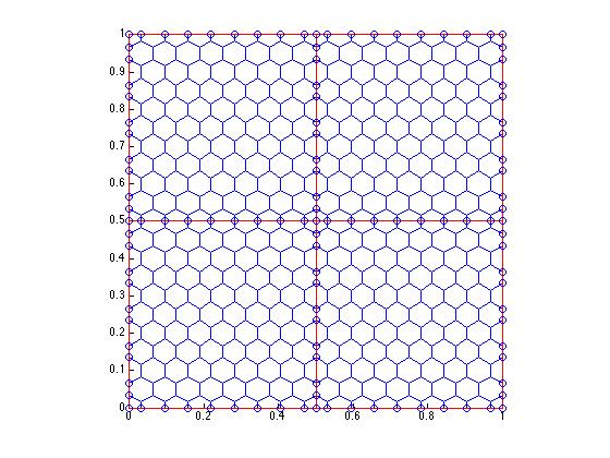
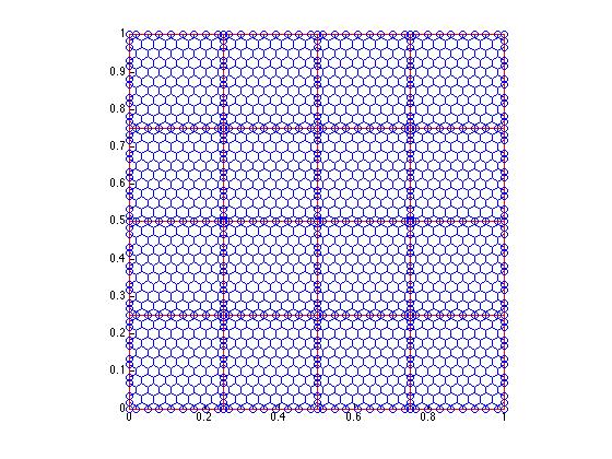
Figure 1. Initial grid of hexagons on a subdomain partition made by $2\times 2$ squares (left) and $4\times 4$.

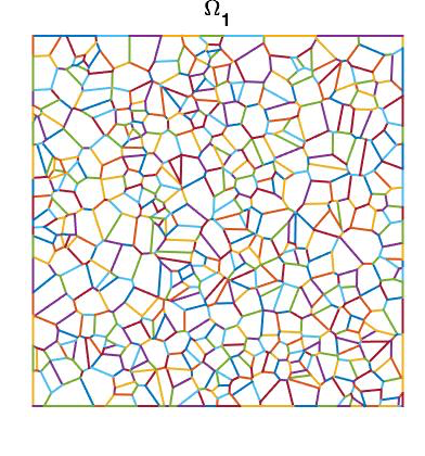
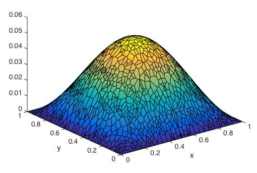
Figure 2. Voronoi mesh in each subdomain. Left. Mesh in $\Omega_{1}$. Right Computed solution with FETI-DP preconditioner.

Table 1. Hexagonal mesh. Number of iterations and condition number of the FETI-DP preconditioned system preconditioners for varying number of subdomains in each coordinate direction $N$ and local problem size $n$.

$N\backslash n$	$8\times 10$	$18\times 20$	$34\times 40$	$70\times 80$
$8$	9 (3.61)	11 (4.81)	11 (5.86)	12 (7.14)
$16$	9 (3.71)	11 (4.92)	12 (5.99)	14 (7.40)
$32$	9 (3.75)	10 (4.95)	11 (6.02)	13 (7.49)
$64$	8 (3.76)	9 (4.96)	10 (6.03)	–

Table 2. Hexagonal mesh. Number of iterations and condition number of the BDDC preconditioned system preconditioners for varying number of subdomains in each coordinate direction $N$ and local problem size $n$.

$N\backslash n$	$8\times 10$	$18\times 20$	$34\times 40$	$70\times 80$
$8$	10 (3.64)	11 (4.81)	11 (5.86)	12 (7.14)
$16$	9 (3.71)	11 (4.92)	12 (5.99)	14 (7.41)
$32$	9 (3.75)	10 (4.95)	12 (6.03)	13 (7.49)
$64$	8 (3.77)	10 (4.97)	10 (6.03)	–

Table 3. Voronoi mesh. Number of iterations and condition number of the FETI-DP preconditioned system preconditioners for varying number of subdomains in each coordinate direction $N$ and local problem size $n$.

$N\backslash n$	$100$	$400$	$1400$	$5000$
$8$	9 (2.88)	11 (3.98)	11 (4.90)	12 (5.67)
$16$	9 (2.94)	12 (4.06)	12 (5.02)	12 (5.79)
$32$	9 (2.95)	11 (4.07)	11 (5.05)	12 (5.82)
$64$	9 (2.96)	11 (4.08)	11 (5.06)	-

6.2. Discontinuous coefficients $\rho$ across the skeleton.

In order to verify the robustness of the method with respect to strong variations of the coefficient $\rho$, we next consider problems with $\rho$ discontinuous across the interfaces $\Gamma$. Inside each subdomain, we consider virtual elements of order $k=1$. Since the BDDC and FETI-DP spectra coincide, we only report the results for FETI-DP. We perform two set of tests. In Test A, the coefficient $\rho$ is equal to 1 except in a square at the center of $\Omega$, where it assumes a constant value $\rho_{0}$ (see Figure 3-Left). Tests are performed for $\rho_{0}=10^{-4},\,10^{-2},\,1,10^{2},10^{4}$. In Test B, $\rho$ takes the value $\rho=10^{\alpha}$, where, for each subdomain, the value of the exponent $\alpha$ is a random integer belonging to $[-4,\dots,4]$ (see Figure 3-Right). In order to test the robustness of the method, for both test cases we chose, as load term $\hat{\mathbf{f}}$ a uniformly distributed random vector.

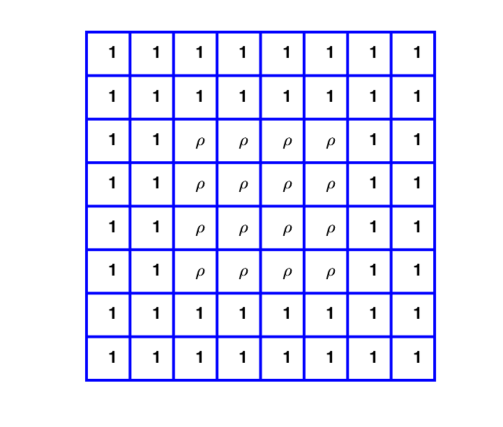
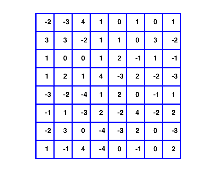
Figure 3. Left : values of the discontinuous coefficient $\rho$ in Test A. Right: random distribution of the exponent $\alpha\in[-4,\dots,4]$ for the elliptic coefficient $\rho=10^{\alpha}$ in Test B.

Table 4. Number of iterations and extreme eigenvalues of unpreconditioned CG and the FETI-DP preconditioned systems for two tests problems (A and B) with discontinuous coefficients $\rho_{i}$ shown in Figure 3.

Test	$\rho$	Unpreconditioned			FETI-DP
		it.	$\lambda_{min}$	$\lambda_{max}$	it.	$\lambda_{min}$	$\lambda_{max}$
A	$10^{-4}$	145	2.54	3.104e5	9	1.01	3.57
	$10^{-2}$	124	1.36	3.104e3	9	1.01	3.58
	$1$	25	1.34	32.58	9	1.02	3.67
	$10^{2}$	110	1.43e-2	27.61	9	1.02	3.58
	$10^{4}$	109	3.83e-4	27.60	9	1.02	3.57
B	$10^{\alpha}$	$>1000$	-	-	9	1.00	3.70

In Table 4 we present the results for Test A and B for a fixed decomposition made of $N=8$ subdomains in each coordinate direction and $n=8\times 10$ hexagons in each subdomain $\Omega_{\ell}$. The results confirm that the convergence rate of FETI-DP is quite insensitive to the coefficient jumps, with iteration counts equal to 9 and minimum eigenvalues very close to 1. In contrast, CG without FETI-DP preconditioner is significantly affected by the increasing jumps: in the first test the condition number is of order $10^{5}$ for both $\alpha=10^{-4}$ and $\alpha=10^{4}$, and CG does not converge within 1000 iterations in Test B.

Table 5. Hexagonal mesh. Number of iterations and condition numbers of the FETI-DP preconditioned system for varying number of subdomains in each coordinate direction $N$ and local problem size $n$. Random distribution of the exponent $\alpha\in[-4,\dots,4]$ in the elliptic coefficient $\rho=10^{\alpha}$.

$N\backslash n$	$8\times 10$	$18\times 20$	$34\times 40$	$70\times 80$
$8$	10 (3.27)	11 (4.16)	13 (5.14)	15 (6.58)
$16$	11 (3.28)	13 (4.21)	15 (5.28)	16 (6.79)
$32$	11 (3.34)	13 (4.36)	15 (5.25)	16 (6.73)

Table 6. Voronoi mesh. Number of iterations and condition numbers of the FETI-DP preconditioned system for varying number of subdomains in each coordinate direction $N$ and local problem size $n$. Random distribution of the exponent $\alpha\in[-4,\dots,4]$ in the elliptic coefficient $\rho=10^{\alpha}$.

$N\backslash n$	$100$	$400$	$1400$	$5000$
$8$	9 (3.07)	11 (4.10)	12 (4.96)	12 (5.73)
$16$	10 (3.08)	12 (4.19)	13 (4.89)	15 (6.00)
$32$	10 (3.00)	12 (4.24)	13 (5.01)	15 (5.85)

In Table 5 and 6 we report the iteration counts and condition numbers of the FETI-DP preconditioned system (5.5) for increasing $N$ (number of subdomains in each coordinate direction) and $n$ (number of elements per subdomain) for Test B. Tables 5 and 6 refer to the case of hexagonal and Voronoi meshes, respectively. The results are consistent with the theoretical bound on the condition numbers (see Corollary (4.3)), i.e. we have a polylogarithmic dependence of the convergence rate on $H/h$ not affected by the jump in the coefficients $\rho$.

6.3. High-order elements.

Finally, we present some computations performed with high-order elements. We take $\rho=1$ and $f=\sin(\pi x)\sin(\pi y)$. Table 7 shows the number of iterations and the maximum eigenvalue $\lambda_{\max}$ for the FETI-DP preconditioned system, for fixed local mesh size ($n=8\times 10$ hexagons) but varying both the polynomial degree $k$ from 2 to 8, and the number of subdomains in each coordinate direction $N$ from $8$ to $32$. The minimum eigenvalue is not reported since it is always very close to 1. The BDDC results are analogous and therefore not displayed.

In Figure 4-Left, it is possible to verify the polylogarithmic dependence of the condition number on the polynomial order $k$, as predicted by the theoretical bound (4.3). Indeed, for $H/h$ fixed, the expected bound $(1+\log(k^{2}H/h)^{2}\sim(1+log(k^{2}))^{2}\sim(1+2\log(k))^{2}$ is a linear semilog plot of the square root of $\lambda_{\max}$. In Figure 4-Right, we keep the polynomial degree fixed to $k=4$ and $k=8$ and increase $H/h$, that is the number of interior elements in each subdomain is increased from $8\times 10$ to $18\times 20$. The largest eigenvalue and thus the condition number behaves as expected and the $(1+log(k^{2}H/h))^{2}\sim(1+log(H/h))^{2}$ bound (for fixed $k$) is confirmed.

Table 7. Number of iterations and maximum eigenvalues of the FETI-DP preconditioned system for fixed local problem size ($n=8\times 10$ hexagons) but increasing polynomial order $k$ and subdomain partitions in each coordinate direction $N$.

$N\backslash k$	2	3	4	5	6	7	8
$8$	11 (5.72)	12 (7.51)	13 (8.56)	13 (9.62)	14 (10.74)	14 (11.50)	14 (12.19)
$16$	12 (5.85)	14 (7.67)	14 (8.72)	15 (9.90)	16 (10.86)	17 (11.74)	17 (12.44)
$32$	11 (5.88)	13 (7.70)	14 (8.90)	14 (10.01)	14 (10.96)	16 (11.81)	-

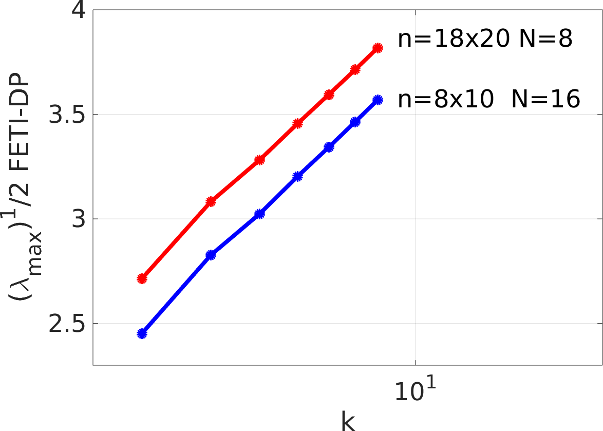
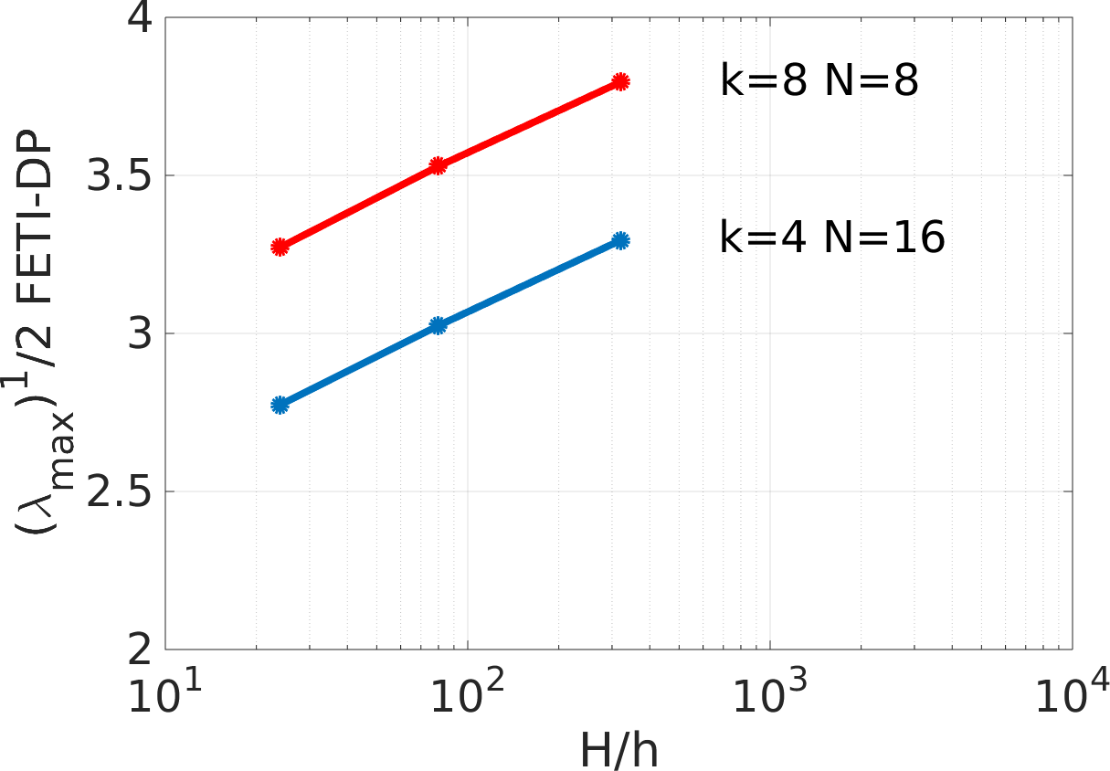
Figure 4. Left. Square root of the largest eigenvalue $\sqrt{\lambda_{\max}}$ for increasing polynomial degree, $n=18\times 20$, $N=8$ and $n=8\times 10$, $N=16$. Right. Square root of the largest eigenvalue $\sqrt{\lambda_{\max}}$ for increasing $H/h$ and $k=4,8$, $N=16,8$.

References

• [1] P. F. Antonietti, A. Cangiani, J. Collis, Z. Dong, E. H. Georgoulis, S. Giani, and P. Houston, Review of discontinuous Galerkin finite element methods for partial differential equations on complicated domains, Connections and Challenges in Modern Approaches to Numerical Partial Differential Equations, Springer, 2016, pp. 279–308.
• [2] P. F. Antonietti, L. Beirão da Veiga, D. Mora, and M. Verani, A stream virtual element formulation of the Stokes problem on polygonal meshes, SIAM Journal on Numerical Analysis 52 (2014), no. 1, 386–404.
• [3] P. F. Antonietti, L. Beirão da Veiga, S. Scacchi, and M. Verani, A $C^{1}$ virtual element method for the Cahn-Hilliard equation with polygonal meshes, SIAM Journal on Numerical Analysis 54 (2016), no. 1, 34–56.
• [4] P. F. Antonietti, L. Mascotto, and M. Verani, A multigrid algorithm for the $p$-version of the virtual element method, arXiv e-prints (2017).
• [5] L. Beirão da Veiga, F. Brezzi, A. Cangiani, G. Manzini, L. D. Marini, and A. Russo, Basic principles of virtual element methods, Mathematical Models and Methods in Applied Sciences 23 (2013), no. 1, 199–214.
• [6] L. Beirão da Veiga, F. Brezzi, and L. Marini, Virtual elements for linear elasticity problems, SIAM Journal on Numerical Analysis 51 (2013), no. 2, 794–812.
• [7] L. Beirão da Veiga, F. Brezzi, L. D. Marini, and A. Russo, The Hitchhiker’s guide to the virtual element method, Mathematical Models and Methods in Applied Sciences 24 (2014), no. 8, 1541–1573.
• [8] L. Beirão da Veiga, F. Brezzi, L. D. Marini, and A. Russo, Mixed virtual element methods for general second order elliptic problems on polygonal meshes, ESAIM: M2AN 50 (2016), no. 3, 727–747.
• [9] L. Beirão da Veiga, F. Brezzi, L. D. Marini, and A. Russo, Serendipity Nodal VEM spaces, Computers & Fluids 141 (2016), 2–12.
• [10] L. Beirão da Veiga, F. Brezzi, L. D. Marini, and A. Russo, Virtual Element Method for general second-order elliptic problems on polygonal meshes, Mathematical Models and Methods in Applied Sciences 26 (2016), no. 4, 729–750.
• [11] L. Beirão da Veiga, Lovadina C., and A. Russo, Stability Analysis for the Virtual Element Method, 2016, arXiv:1607.05988.
• [12] L. Beirão da Veiga, A. Chernov, L. Mascotto, and A. Russo, Basic principles of $hp$ virtual elements on quasiuniform meshes, Mathematical Models and Methods in Applied Sciences 26 (2016), no. 8, 1567–1598.
• [13] L. Beirão da Veiga, L. F. Cho, D.and Pavarino, and S. Scacchi, BDDC preconditioners for isogeometric analysis, Mathematical Models and Methods in Applied Sciences 23 (2013), no. 6, 1099–1142.
• [14] L. Beirão da Veiga, K. Lipnikov, and G. Manzini, The mimetic finite difference method for elliptic problems, MS&A, no. 11, Springer, 2014.
• [15] L. Beirão da Veiga, C. Lovadina, and G. Vacca, Divergence free virtual elements for the Stokes problem on polygonal meshes, ESAIM: M2AN 51 (2017), no. 2, 509–535.
• [16] L. Beirão da Veiga, C. Lovadina, and G. Vacca, Virtual Elements for the Navier-Stokes problem on polygonal meshes, arXiv e-prints (2017).
• [17] L. Beirão da Veiga, L. F. Pavarino, S. Scacchi, O. B. Widlund, and S. Zampini, Isogeometric BDDC preconditioners with deluxe scaling, SIAM Journal on Scientific Computing 36 (2014), no. 3, A1118–A1139.
• [18] M. F. Benedetto, S. Berrone, and S. Scialó, A globally conforming method for solving flow in discrete fracture networks using the virtual element method, Finite Elements in Analysis and Design 109 (2016), 23 – 36.
• [19] S. Berrone and A. Borio, Orthogonal polynomials in badly shaped polygonal elements for the Virtual Element Method, Finite Elements in Analysis and Design 129 (2017), 14–31.
• [20] S. Bertoluzza, Substructuring preconditioners for the three fields domain decomposition method, Math. Comp. 73 (2004), no. 246, 659–689.
• [21] J. H. Bramble, J. E. Pasciak, and A. H. Schatz, The construction of preconditioners for elliptic problems by substructuring, I, Math. Comp. 47 (1986), no. 175, 103–134.
• [22] J. H. Bramble, J. E. Pasciak, and A. H. Schatz, The construction of preconditioners for elliptic problems by substructuring, IV, Math. Comp. 53 (1989), 1–24.
• [23] S. C. Brenner and L. R. Scott, The mathematical theory of finite element methods, Texts in Applied Mathematic, no. 15, Springer, 2008.
• [24] S. C. Brenner and L. Y. Sung, BDDC and FETI-DP without matrices or vectors, Computer Methods in Applied Mechanics and Engineering 196 (2007), no. 8, 1429 – 1435.
• [25] F. Brezzi, K. Lipnikov, and M. Shashkov, Convergence of mimetic finite difference methods for diffusion problems on polyhedral meshes, SIAM Journal on Numerical Analysis 43 (2005), 1872–1896.
• [26] A. Cangiani, E. H. Georgoulis, and P. Houston, hp-version discontinuous Galerkin methods on polygonal and polyhedral meshes, Mathematical Models and Methods in Applied Sciences 24 (2014), no. 10, 2009–2041.
• [27] C. Canuto, Stabilization of spectral methods by finite element bubble functions, Comput. Methods Appl. Mech. Engrg. 116 (1994), 13–26.
• [28] C. Canuto, L. P. Pavarino, and A. B. Pieri, BDDC preconditioners for continuous and discontinuous Galerkin methods using spectral/hp elements with variable local polynomial degree, IMA Journal of Numerical Analysis 34 (2014), no. 3, 879–903.
• [29] B. Cockburn, B. Dong, and J. Guzmán, A superconvergent LDG-hybridizable Galerkin method for second-order elliptic problems, Mathematics of Computation 77 (2008), no. 264, 1887–1916.
• [30] L. Beirão da Veiga, C. Lovadina, and D. Mora, A virtual element method for elastic and inelastic problems on polytope meshes, Computer Methods in Applied Mechanics and Engineering 295 (2015), 327 – 346.
• [31] D. A. Di Pietro and A. Ern, Hybrid high-order methods for variable-diffusion problems on general meshes, Comptes Rendus Mathèmatique 353 (2015), no. 1, 31–34.
• [32] C. R. Dohrmann, A preconditioner for substructuring based on constrained energy minimization, SIAM Journal on Scientific Computing 25 (2003), no. 1, 246–258.
• [33] M. Dryja, J. Galvis, and M. Sarkis, BDDC methods for discontinuous Galerkin discretization of elliptic problems, Journal of Complexity 23 (2007), no. 4, 715–739.
• [34] C. Farhat, M. Lesoinne, P. LeTallec, K. Pierson, and D. Rixen, FETI-DP: A Dual-Primal unified FETI method - Part I: A faster alternative to the two-level FETI method, International Journal for Numerical Methods in Engineering 50 (2001), 1523–1544.
• [35] M. Frittelli and I. Sgura, Virtual Element Method for the Laplace-Beltrami equation on surfaces, arXiv e-prints (2016).
• [36] A. L. Gain, C. Talischi, and G. H. Paulino, On the virtual element method for three-dimensional linear elasticity problems on arbitrary polyhedral meshes, Computer Methods in Applied Mechanics and Engineering 282 (2014), 132–160.
• [37] G. H. Golub and C. F. Van Loan, Matrix computations, third ed., Johns Hopkins Studies in the Mathematical Sciences, Johns Hopkins University Press, Baltimore, MD, 1996.
• [38] H. H. Kim, A BDDC algorithm for mortar discretization of elasticity problems, SIAM Journal on Numerical Analysis 46 (2008), no. 4, 2090–2111.
• [39] H. H. Kim,  A FETI-DP formulation of three dimensional elasticity problems with mortar discretization, SIAM Journal on Numerical Analysis 46 (2008), no. 5, 2346–2370.
• [40] H. H. Kim, M. Dryja, and O. B. Widlund, A BDDC method for mortar discretizations using a transformation of basis, SIAM Journal on Numerical Analysis 47 (2008), 136–157.
• [41] H. H. Kim and X. Tu, A three-level BDDC algorithm for mortar discretization, SIAM Journal on Numerical Analysis 47 (2009), 1576–1600.
• [42] A. Klawonn, M. Lanser, and O. Rheinbach, A highly scalable implementation of inexact nonlinear FETI-DP without sparse direct solvers, pp. 255–264, Springer International Publishing, 2016.
• [43] A. Klawonn, M. Lanser, O. Rheinbach, H. Stengel, and G. Wellein, Hybrid MPI/OpenMP parallelization in FETI-DP methods, pp. 67–84, Springer International Publishing, 2015.
• [44] A. Klawonn, L. F. Pavarino, and O. Rheinbach, Spectral element FETI-DP and BDDC preconditioners with multi-element subdomains, Computer Methods in Applied Mechanics and Engineering 198 (2008), no. 3, 511–523.
• [45] A. Klawonn and O. Rheinbach, Highly scalable parallel domain decomposition methods with an application to biomechanics, ZAMM-Z. Angew. Math. Mech. 90 (2010), 5–32.
• [46] A. Klawonn and O. B. Widlund, Dual-primal FETI methods for linear elasticity, Communications on Pure and Applied Mathematics 59 (2006), no. 11, 1523–1572.
• [47] J. Li and O. Widlund, FETI-DP, BDDC and block cholesky methods, International Journal for Numerical Methods in Engineering 66 (2006), no. 2, 250–271.
• [48] J. Mandel, C. R. Dohrmann, and R. Tezaur, An algebraic theory for primal and dual substructuring methods by constraints, Applied Numerical Mathematics 54 (2005), no. 2, 167 – 193.
• [49] J. Mandel and B. Sousedík, BDDC and FETI-DP under minimalist assumptions, Computing 81 (2007), no. 4, 269–280.
• [50] L. Mascotto, A therapy for the ill-conditioning in the virtual element method, arXiv e-prints (2017).
• [51] L. Mascotto, L. Beirão da Veiga, A. Chernov, and A. Russo, Exponential convergence of the hp Virtual Element Method with corner singularities, arXiv e-prints (2016).
• [52] D. Mora, G. Rivera, and R. Rodríguez, A virtual element method for the Steklov eigenvalue problem, Mathematical Models and Methods in Applied Sciences 25 (2015), no. 8, 1421–1445.
• [53] L. F. Pavarino, BDDC and FETI-DP preconditioners for spectral element discretizations, Computer Methods in Applied Mechanics and Engineering 196 (2007), no. 8, 1380–1388.
• [54] I. Perugia, P. Pietra, and A. Russo, A plane wave virtual element method for the Helmholtz problem, ESAIM: M2AN 50 (2016), no. 3, 783–808.
• [55] D. S. Rjasanow and S. Weißer, Higher order BEM-based FEM on polygonal meshes, SIAM Journal on Numerical Analysis 241 (2013), 103–115.
• [56] B. F. Smith, A domain decomposition algorithm for elliptic problems in three dimensions, Numer. Math. 60 (1991), no. 2, 219–234.
• [57] N. Sukumar and A. Tabarraei, Conforming polygonal finite elements, International Journal for Numerical Methods in Engineering 61 (2004), no. 12, 2045–2066.
• [58] A. Toselli and O. Widlund, Domain decomposition methods - algorithms and theory, Springer Series in Computational Mathematics, vol. 34, Springer, 2004.
• [59] G. Vacca and L. Beirão da Veiga, Virtual element methods for parabolic problems on polygonal meshes, Numerical Methods for Partial Differential Equations 31 (2015), no. 6, 2110–2134.
• [60] J. Wang and X. Ye, A weak Galerkin finite element method for second-order elliptic problems, Journal of Computational and Applied Mathematics 241 (2013), 103–115.