Solar coronal lines in the visible and infrared. A rough guide

Abstract

We review the coronal visible and infrared lines, collecting previous observations, and comparing, whenever available, observed radiances with those predicted by various models: the quiet Sun, a moderately active Sun, and an active region as observed near the limb, around 1.1 $\rm R_{\odot}$. We also model the off-limb radiances for the quiet Sun case. We used the most up-to-date atomic data in CHIANTI version 8. The comparison is satisfactory, in that all of the strong visible lines now have a firm identification. We revise several previous identifications and suggest some new ones. We also list the large number of observed lines for which we do not currently have atomic data, and therefore still await firm identifications. We also show that a significant number of coronal lines should be observable in the near-infrared region of the spectrum by the upcoming Daniel K. Inouye Solar Telescope (DKIST) and the AIR-Spec instrument, which observed the corona during the 2017 August 21 solar eclipse. We also briefly discuss the many potential spectroscopic diagnostics available to the visible and infrared, with particular emphasis on measurements of electron densities and chemical abundances. We briefly point out some of the potential diagnostics that could be available with the future infrared instrumentation that is being built for DKIST and planned for the Coronal Solar Magnetism Observatory (COSMO). Finally, we highlight the need for further improvements in the atomic data.

1. Introduction

Within the solar community, there is currently renewed interest in the coronal forbidden lines in the visible and infrared, partly because several breakthrough observations are forthcoming. For example, the Daniel K. Inouye Solar Telescope (DKIST, see Rimmele et al. 2015), formerly known as ATST (Keil et al., 2003), will carry out ground-breaking observations of the solar corona with its 4 meter telescope on Haleakala, Maui with two dedicated coronagraphs. It will begin operations in 2019 and will carry out routine daily observations up to 1.5 $\rm R_{\odot}$  in selected wavelength regions between about 5000 Å and 5 $\mu$m with the CryoNIRSP spectropolarimeter (Fehlmann et al., 2016). In its coronagraphic mode, the instrument will have a resolution of 30,000, a spatial resolution of 0.5″, and a field of view (FOV) of 4′ $\times$3′, equivalent to the size of an active region. The FOV will be scanned with high cadence using a multislit. In addition, global scale coronal magnetic field measurements are the focus of the proposed Coronal Solar Magnetism Observatory (COSMO), see Tomczyk et al. (2016).

The longer wavelengths of the infrared spectral region are still largely unexplored, but there is a lot of interest in this spectral region, and in the near future several new observations, aside from DKIST, will become available. For example, the airborne infrared spectrometer (AIR-Spec), described by DeLuca et al. (2016), was built to carry out observations in the infrared during the 2017 August 21 solar eclipse, on-board an high-altitude airplane. The instrument was designed to observe four spectral regions (2.82–3.07 $\mu$m and 3.74–3.98 $\mu$m in first order), and five coronal lines: Si x 1.43 $\mu$m, S xi 1.92 $\mu$m, Fe ix 2.86 $\mu$m, Mg viii 3.03 $\mu$m, and Si ix 3.93 $\mu$m. Preliminary analysis (Samra 2017 private communication) suggests that all of the lines were successfully observed.

One might ask: what could observations of the coronal visible and infrared lines provide, given the abundance of current EUV and UV observations?

The importance of the infrared observations for measuring the coronal magnetic field has been recognised for a long time, see e.g. the Living Review by Penn (2014). Judge (1998) carried out simulations to predict which of the visible and infrared coronal lines, should be observable, with an emphasis on the infrared ones which could be used to measure magnetic fields. Judge et al. (2013) discussed some specific issues related to DKIST.

The forbidden lines are also useful for many other diagnostics, aside from the potential to measure coronal magnetic fields. For example, plasma flows and line widths can be measured with an accuracy far superior to that of any other wavelength. There is an extended literature on the non-thermal widths of the lines, which in principle provide important constraints to coronal heating theories.

Another example concerns the possibility to provide direct measurements of electron temperatures and constrain for the presence of non-Maxwellian electron distributions (Dudík et al., 2014), when combined with measurements in the UV or EUV. Such diagnostics have been attempted in the EUV (Dudík et al., 2015), but are very difficult.

For a general review on the diagnostic potential of the forbidden lines from ground-based observations see Landi et al. (2016). In their review, future ground-based instrumentation is also briefly presented, with emphasis on UCoMP and COSMO. UCoMP is an upgraded version of the Coronal Multichannel Polarimeter (CoMP) instrument, described by Tomczyk et al. (2008). UCoMP will be a pathfinder for a Large 1.5 m refractive Coronagraph (LC), which is currently in its advanced planning phase, and forms part of a suite of ground-based telescopes, COSMO, which will be built to study the outer corona. The current design of the COSMO LC calls for a tunable filter focal plane instrument operating between 500-1100nm. The baseline covers cool CME core lines (H i, He i, Ca ii, O ii, O iii, and Fe iv), hot lines (Fe xiv, Fe xv, S xii, Ar xiii and Ca xv) and lines in the quiescent corona (Fe x, Fe xi, Fe xiii, Fe xiv, Ar x, and Ar xi). The spatial resolution of COSMO LC is 2” and the FOV covers a full degree. We can see that it will be an excellent complement to DKIST providing a high magnetic sensitivity (1G), temperature coverage and global coronal coverage.

In the present paper, we limit our discussion to diagnostic techniques of line intensity ratios which can be used to measure the electron density and relative elemental abundances.

As already pointed out by Woolley & Allen (1948), the visible lines allow a direct measurement of the absolute (i.e. relative to hydrogen) values of the chemical abundances, by comparing line radiances with the continuum.

It is well-known that coronal abundances can be different from the photospheric ones, and that correlations exist between the abundance of an element and its first ionization potential (FIP). The low-FIP ($\leq$ 10 eV) elements are more abundant than the high-FIP ones, relative to their photospheric values. See, e.g. the Living Review by Laming (2015). The FIP effect is now considered an important issue, because it can help to trace the in-situ solar wind measurements to the source regions, an important topic for the upcoming Solar Orbiter (to be launched in early 2019), which will measure elemental abundances with both in-situ and remote-sensing instruments. Relative abundances are comparatively easier to measure and there are plenty of observations in the X-ray, EUV, and UV. Absolute values are harder to obtain, and in the literature there are plenty of contradictory results. In fact, it is not well-accepted if low-FIP elements are over-abundant, or the high-FIP ones are depleted, compared to the photospheric values. There are SoHO SUMER and UVCS measurements relative to hydrogen lines, but a direct measurement against the continuum is only available in the X-rays during flares. Therefore, line-to-continuum measurements of the forbidden lines in the visible and infrared have a potential to resolve these issues, although we should point out that an instrument such as DKIST will only measure the polarized component of the continuum, and not the total continuum.

Aside from all the above diagnostic possibilities, the forbidden lines are also very useful just to trace the open and closed structures in the outer corona. The forbidden lines are very sensitive to photoexcitation of the disk brightness, at the low densities of the outer corona. Therefore, their intensities are closer to being proportional to the electron density, rather than the square, as is the case for the strong dipole-allowed lines in the EUV. This means that the intensities of the forbidden lines decrease with the radial distance more slowly than those of the EUV lines, hence they show the outer corona to larger distances.

Comparisons of coronal emission lines in the EUV and Vis/IR show enhanced radiative contributions in the visible/IR forbidden lines (Habbal et al., 2010, 2011). Habbal’s work used narrow band filters centered on and off strong emission lines, allowing the continuum contribution to be isolated from the line contribution. Narrow band imaging allows for the exploration of the whole corona during each eclipse observation. The success of her imaging approach motivates our need for an accurate understanding of the visible/IR coronal emission.

It might be surprising, but the visible and infrared regions of the coronal spectrum are largely unexplored. This is mainly due to the paucity of observations. Interestingly, the same problem concerns the soft X-rays, between 60 and 170 Å. The two spectral regions are historically related: Edlén’s pioneering laboratory measurements of soft X-ray spectra in the 1930s and identifications of lines from iron and other elements allowed Grotrian (1939) to identify the famous bright red coronal forbidden line at 6374.6 Å as the Fe x transition ²P_3/2–²P_1/2 within the ground configuration. Edlén then wrote a seminal paper (Edlén, 1943), confirming that the solar corona is a million degree plasma (see also Swings 1943 for more details). Edlén work was extended by Fawcett et al. (1972), and recently revised by Del Zanna (2012a), where the strongest lines in the soft X-ray spectra, which were previously unknown, have been identified. This was only possible because of large-scale atomic calculations for the main iron and nickel coronal ions which were recently carried out within the UK APAP network, the main provider of atomic data for fusion and astrophysical plasma. However, a large number of lines in the soft X-rays are still unidentified.

In the literature, contradicting line identifications of the visible lines are common, even for some among the strongest lines. A large number of authors have contributed to the identifications over the years. Among those: Edlén, Svensson, Ekberg, Smitt, Mason, Nussbaumer, Magnant-Crifo, just to name a few. Most of the suggested identifications were mainly based on wavelength coincidences along isoelectronic sequences, and sometimes with approximate estimates of the line intensities. One exception among the early studies is the work of Mason & Nussbaumer (1977), where the excitation cross section for Fe x and Fe xi were actually calculated, allowing more accurate estimates of line intensities. This enabled the authors to suggest, also on intensity grounds, several new identifications for these two important ions.

It might be surprising, but accurate atomic rates for the forbidden lines have only been recently available for a number of ions. The main ions producing the strongest forbidden lines are from Iron, and the above-mentioned large-scale atomic calculations have produced significantly different results. For example, as shown in Del Zanna et al. (2014), significant differences (factors of 2) were found for some of the forbidden lines of Fe ix and Fe x, compared to earlier (but still sophisticated) calculations. Most of these data have been included in CHIANTI version 8 (Del Zanna et al., 2015), which is used here. We note that Judge (1998) used the atomic data available at the time, i.e. CHIANTI version 1 (Dere et al., 1997).

It is therefore timely to review all the observations of the forbidden lines with the latest atomic data. Our main aim of this paper is to provide a comprehensive list of the main lines observed, and assess their identification on the basis of the current atomic data. A full benchmark of the atomic data along the lines of the series of papers which started with Del Zanna et al. (2004) is not possible at this time, given the uncertainties in the calibrated radiances of the visible and infrared lines. Many identifications will need to be confirmed with future observations.

Our aim is also to provide rough estimates of line radiances for different activity conditions, and as a function of distance, to aid the planning of future observations. In particular, the present results were used to aid the planning of the AIR-Spec infrared observations. Finally, we also provide some examples of which spectral lines would be suitable for measuring electron densities and elemental abundances, using intensity ratios.

2. Observations

In this section, we briefly review only the main observations we have used for the present assessment, and which contained published spectral observations where wavelengths and/or line radiances were provided. In other words, this section is not meant to even summarise the large volume of literature on ground- and space-based observations of the forbidden lines, especially during total eclipses.

2.1. Observations in the visible

The genius of Bernard Lyot made breakthrough observations of the coronal visible and near infrared lines with a novel coronagraph outside eclipses. He carried out observations at the Pic du Midi Observatory, observing 11 coronal lines, some for the first time (Lyot, 1939). In many respects, his observations are still unsurpassed. Lyot also classified the lines into three groups, following their intensity distributions in the corona. The three representatives of the groups were the red Fe x, the green Fe xiv, and the yellow Ca xv. We now know that this simple classification reflects the temperature of formation of these ions, and it is a very useful information when trying to identify a spectral line. This scheme was somewhat complicated later on by Shajn (1948) and following authors with the introduction of a fourth class. So after Van de Hulst (1953), it has been customary to assign lines from ions such as Fe x a class I, those like Fe xiii and Fe xiv a class II, the Ca xiii and Ni xvi a class III, while all the hotter ions such as Ca xv and Fe xv, only visible in active regions, were given a class IV.

We note that in the literature it was common to name the bright hot regions in the solar corona as ‘condensations’. In the present paper, we refer to them as active regions, because that is what they were. We also note that we only consider here coronal lines formed around 1 MK or more, and not chromospheric lines.

There are many historical observations of coronal lines during eclipses. An early one worth a special mention is the Harvard-MIT expedition to the 1936 eclipse. The expedition recorded spectra in the near-ultraviolet and visible with three instruments. Petrie & Menzel (1942) provided an extensive list of lines, some of which have not been observed since, hence should be considered with caution. We only report the coronal lines that they considered more certain. A complete review list of 27 well-observed coronal lines known at the time was provided by Van de Hulst (1953).

We now briefly review the main observations we have assessed, starting with the two most important eclipses. The present study extends the excellent list of observed visible lines compiled by Mouradian (1997), by adding other observations. It is also an improvement in that several of the identifications listed by Mouradian (1997) turned out to be incorrect.

2.1.1 The 1952 February 25 eclipse

Lyot designed a novel instrument with a circular slit, and built two spectrographs, one in the visible and one in the near ultraviolet, to observe the 1952 February 25 eclipse at Khartoum, Egypt, with the assistance of Aly. They obtained the best ever plates of the coronal lines. They were also lucky in that a very extended, hot and high-density active region was located at the limb. Next to it, a large prominence was also present, which was key to obtain accurate measurements of the coronal lines using as a reference the known chromospheric lines, which were very strong in the prominence.

Unfortunately, Lyot only managed to perform an initial analysis and died in Egypt three months after. The results of this initial analysis are reported in Lyot & Aly (1955) as a first Table. Aly subsequently added several weaker lines, and added a second Table in the same publication. A preliminary photometric analysis of the plates was later carried out in Meudon by Divan & Pecker (1960), while a further analysis and line intensities were provided in Aly et al. (1962a). We adopt in our Table 2 the calibrated radiances at the center of the active region, as listed by Jefferies et al. (1969) (see below). As Aly et al. (1962a) described, the relative calibration was quite accurate, because it could be checked against the observed continuum. However, the absolute values are uncertain by about a factor of two. The distance from the limb was also quite uncertain, but should range between 1.05 and 1.1 $\rm R_{\odot}$, with 1.09 $\rm R_{\odot}$as the quoted value.

The plates were subsequently taken to Sac Peak and re-analysed by Aly, Evans and Orrall independently, as described in Aly et al. (1962b). The lines were given a class, on the basis of the certainty in the identification of a line as a coronal line in the plates, which was not trivial. The well-known lines were given an ’A’. The well-observed ones were given a class ’B’, while those more difficult to measure were listed as ’C’. The dubious ones were given a class ’D’. Several of the lines originally listed by Aly et al. (1962a) in the second table were subsequently listed as dubious by Aly et al. (1962b). In our Tables 2,3 below we typically list only the lines in the A,B,C classes as in the Aly et al. (1962b) report.

The wavelengths are often given with a decimal figure, but appear to be uncertain by about 1–3 Å, as it appears from a comparison with subsequent observations. This means that in several instances it is not clear if more lines have been observed or just the wavelengths reported were inaccurate. When the differences are more than 1 Å we list the wavelengths reported by Aly.

Lyot’s observations had a profound influence in many areas. They showed that it is possible to measure the absolute abundances (i.e. relative to hydrogen) of the observed elements. This was carried out by Pottasch (1964) with these data, and later by several authors with these and other datasets (see, e.g. Magnant-Crifo, 1974; Mason, 1975b)

Lyot’s observations prompted M.J. Seaton at University College London (UCL) to challenge H.E. Mason to provide the first accurate scattering calculations for the coronal iron ions (Mason, 1975a). The calculations used the state-of-the-art UCL Distorted Wave (DW) scattering codes, mainly developed by W. Eissner and M.J. Seaton (Eissner & Seaton, 1972). These calculations allowed for the first time one to predict line intensities. It was shown that cascading is an important effect when estimating the intensities of the forbidden lines. These codes have been widely used since for the calculations of atomic data in general for astrophysics.

2.1.2 The 1965 May 30 eclipse

Two spectrographs similar to the one used by Lyot (with a circular slit) were built by the Sac Peak and University of Hawaii groups under the supervision of Dunn (Dunn, 1966), to observe the 1965 May 30 eclipse. One spectrograph was aboard a NASA aircraft and recorded spectra in the visible from 3000 to 9000 Å. The other spectrograph obtained ground-based simultaneous observations from the Bellingshauen Island.

The spectra were dominated by the presence of an active region, which however was not as bright and hot as that one observed by Lyot in 1952. Curtis et al. (1965) presented a complete list of wavelengths and identifications based on the flight spectra. We adopt it as the basis of our Tables 2,3 for the lines in the 3000 to 9000 Å range. The estimated accuracy is about 0.4 Å. We have converted the air wavelengths measured by Curtis to vacuum wavelengths following Edlén (1966). The Lyot class of the observed lines is also reported in the Tables, whenever available.

Jefferies et al. (1971) provided a well-cited list of line radiances obtained from the ground at two slit positions. The wavelengths listed by Jefferies et al. (1971) are those reported by Curtis et al. (1965).

As discussed by Jefferies et al. (1969), the same instrument obtained good spectra at the 1966 eclipse in Bolivia. Jefferies et al. (1969) provides a list of calibrated radiances of the 1965 and and 1966 eclipse, as well as radiances in the core of the active region of the 1952 eclipse. This comparison is really important, as it shows that the AR observed by Lyot in 1952 was unusually bright and hot. Indeed lines such as Ca xv were not observed in the 1965 and 1966 eclipses.

Several identifications listed by Curtis et al. (1965) and Jefferies et al. (1971) turn out to be incorrect, as discussed by various authors later on. In most cases, lines were actually due to Iron ions. Most of the correct identifications are reported in the review by Smitt (1977), although the actual original identifications are due to many authors.

Magnant-Crifo (1973) later performed a detailed analysis of the flight spectra of the 1965 eclipse. They were taken at radial distances of about 1.1  $\rm R_{\odot}$. Discrepancies with the radiances obtained from the ground spectra were ascribed to an incorrect measurement of the radial distance of the slit by Jefferies et al. (1971). The useful result of the Magnant-Crifo (1973) analysis is a complete list of line equivalent widths as a function of positon angle and radial distance, from which line intensities can be obtained. We have analysed the intensities at several positions, and noted that an active region dominated the spectra. We selected two regions far away to compare with our estimates (see below).

2.1.3 Other observations

The most remarkable observation of the visible forbidden lines in the red and near-infrared was obtained by Wlérick & Fehrenbach (1963) with the 1.9 meter telescope of Haute provence, which happened to be along the totality path of the famous 1961 February 15 eclipse in Europe. They observed a number of lines never observed since, and provided the best ever wavelength measurements. However, many lines were very weak so we list them with a question mark.

Many other observations have been carried out. We only briefly mention the most notable ones. Kurt (1962) observed the visible spectrum from an aircraft, during the same eclipse of 1961 February 15. Kernoa et al. (1965) report an analysis of other observations taken during the same eclipse. Byard & Kissell (1971) obtained the Fe abundance from observations of the infrared Fe XIII lines during the total eclipse of 12 Nov 1966. Nikolsky et al. (1971) report several new weak unidentified lines observed during the 1970 March 7 eclipse. The wavelengths are not very accurate and most of the weak lines have not been observed by others, so are not reported here. Liebenberg et al. (1975) carried out detailed measurements of the coronal green line.

2.2. Infrared observations

Following the observations of the Fe xiii infrared lines by Lyot (1939), many observations of these and other lines have been carried out in a number of sites, see e.g. Firor & Zirin (1962); Zirin (1970); Fisher & Pope (1971); Querfeld (1977); Arnaud & Newkirk (1987); Singh et al. (2004). More recently, routine observations of the Fe xiii infrared lines have been carried out with the CoMP instrument (Tomczyk et al., 2008) at the Mauna Loa Solar Observatory.

Lines at longer wavelength are intrinsically weaker and difficult to observe from the ground. Münch et al. (1967) reported observations in the infrared, obtained with a spectrograph and a circular slit close to the solar limb, obtained during the 1966 November 12 eclipse from a NASA airborne flight. The Si X 1.43 micron line was observed, as well as the Mg VIII 3.027 micron line. Approximate radiances for these lines were provided. Note that the Si X 1.43 micron line was later also observed with a coronagraph of the National Solar Observatory at Sacramento Peak by Penn & Kuhn (1994).

Olsen et al. (1971) carried out some excellent observations in the infrared between 1 and 3 $\mu$m, obtained during the eclipse of 1970 March 7. The spectrograph was mounted on-board a high-altitude airplane. Approximate line intensities were provided, as well as several identifications. We list below in our Tables 2,3 their measurements, but note that some of the identifications were incorrect, as pointed out later by Kastner (1993).

Kuhn et al. (1996) presented an infrared spectrum obtained during the 1994 solar eclipse. The S IX line at 1.25 $\mu$m was detected, and the Si x 1.43 $\mu$m was also observed. Finally, we note that Judge et al. (2002) detected the Si ix 3.93 $\mu$m line from ground-based observations.

3. Estimates of line radiances near the limb

The Sun is a variable star, and it has always been known even from the early eclipse observations that the solar corona presents completely different characteristics in time and space. To provide a guideline of observable lines and assess the identifications of all the observed lines is a difficult task.

The forbidden lines are extremely sensitive to the electron temperature, density, photoexcitation and chemical abundances. All these parameters change significantly from region to region.

We now have excellent spectroscopic measurements of the inner corona, up to 1.3 $\rm R_{\odot}$, from e.g. SoHO CDS and SUMER, Hinode EIS, and of the outer corona from SoHO UVCS. We therefore have a fairly good understanding of these parameters to be able now to perform some reliable estimates for the forbidden lines.

The easiest case to model is that of the quiet Sun (QS), when no active regions are present. However, very few measurements are available for the coronal lines, as most of the reported observations are on active regions.

In order to provide a rough guide on what radiances are expected when the Sun is more active, we have therefore opted to present the results of two other simulations, one on the brightest active region observed so far (AR) by Lyot in 1952, and one when the Sun was more quiet (QR).

As the forbidden lines are well known to be very sensitive to the photoexcitation, we started by building a photospheric spectrum to be used for the simulations. We opted for the irradiance spectrum compiled by Kurucz (2006), which was based on high-resolution measurements, scaled to agree with the well-calibrated ATLAS-3 spectrum by Thuillier et al. (2004). We supplemented this spectrum with that of a black body at the near-infrared wavelengths. We compared the Kurucz (2006) spectrum to that of a black-body at 6,000 K and to the lower-resolution reference spectrum compiled by Woods et al. (2009), and found some differences, although not too significant for the present purpose.

We assume uniform distribution on disk, i.e. have converted the irradiances to radiances. This is clearly a good assumption for the quiet Sun, but not in the case of the active Sun. We have performed the simulations with and without photoexcitation, to assess which line is most affected. We used the framework developed for CHIANTI version 4 (Young et al., 2003) by P.R. Young to include the photoexcitation in the modelling.

3.1. The QS simulation

SoHO SUMER (see, e.g. Feldman et al. 1997; Landi et al. 2002) and Hinode EIS (see, e.g. Warren & Brooks, 2009; Del Zanna, 2012b) observations of the off-limb quiet Sun have established that the emission measure (EM) distributions are very narrow around 1 MK. This is obtained with the EM loci method (see, e.g. Strong, 1978; Del Zanna et al., 2002), by plotting the ratio of the observed intensity $I_{\rm ob}$ of a line with its contribution function, $I_{\rm ob}/G(T)$, as a function of temperature. The loci of these curves are an upper limit to the emission measure distribution. If the curves cross at one point, that is a strong indication of an isothermal plasma.

There is also good agreement in the absolute values, if one compares e.g. the EM loci curves from EIS and SUMER (Del Zanna, 2012b; Landi et al., 2002). We have chosen as a baseline for our model the SUMER observations reported by Landi et al. (2002), because they include far more ions than the EIS ones. The SUMER spectra were taken between 1.03 and 1.045 $\rm R_{\odot}$. It is well-known from SoHO CDS, SUMER and Hinode EIS observations of line ratios that the electron density is about 2$\times 10^{8}$ (cm^-3), which is what we adopted. We run a simple isothermal model with log $T$ [K]=6.14, log EM=27.1, and the photospheric abundances of Asplund et al. (2009). The observed and predicted SUMER radiances for a selection of strong lines are shown in Table 1.

What is not well established in the literature is the chemical composition of the low corona of the quiet Sun. In most literature, including Landi et al. (2002), it is assumed that in the quiet corona the low-FIP elements are increased by a factor of about 3-4, compared to their photospheric values. However, there is also a body of literature showing no FIP effect in the quiet Sun.

For the purpose of the present estimates, this issue is not relevant, as long as the model is capable of reproducing the observed line intensities. However, it is interesting to note, looking at Table 1, the relatively good agreement for both low- and high-FIP elements. We originally aimed at a factor of two agreement, but in many instances the agreement is far better. We also note that we selected those lines where the atomic data are more reliable. In fact, many of the SUMER lines are forbidden and their intensities are more difficult to calculate. Indeed, for many of the ions observed by SUMER, we still do not have accurate atomic data for all transitions.

Table 1SUMER quiet Sun radiances (erg cm^-2 s^-1 sr^-1) of a selection of lines, as observed (I_obs) by Landi et al. (2002) and predicted (I_pred) with an isothermal assumption and the photospheric abundances of Asplund et al. (2009).

Ion	$\lambda$ (Å)	Iobs	Ipred
Fe x	1463.49	0.84	0.76
Fe xi	1467.07	3.4	3.1
Fe xii	1349.40	5.3	3.4
Mg viii	772.26	0.67	0.42
Mg ix	706.06	8.16	6.0
Mg x	609.79	1.5$\times$102	1.4$\times$102
Si vii	1049.22	0.04	0.03
Si viii	944.47	2.0	1.7
Si ix	950.16	1.9	1.0
Si x	638.93	5.2	3.9
Si xii	520.67	9.2	10.
Ca x	557.77	8.0	10.
High-FIP elements
Ne vii	895.17	0.13	0.18
Ne viii	770.43	30.7	50.
O vi	1037.61	28.5	26.
S ix	871.73	0.44	0.29
S x	776.37	1.9	1.6
S xi	575.0	0.47	0.37
Ar xi	1392.10	0.13	0.11

We used this simple isothermal model to predict the radiances of all the forbidden lines in the visible and infrared. In order to make a meaningful comparison to the eclipse data taken at 1.1 $\rm R_{\odot}$  by Magnant-Crifo (1973), we had to scale these radiances. We estimate (see below) that the radiances would have decreased by about a factor of 2.4 at 1.1 $\rm R_{\odot}$, and have therefore scaled the predicted values by this amount.

We have chosen the scan No. 355 as an example of a quiet region, noting that the 1 MK lines such as Fe x are quite weak, but there are regions where they are even weaker. The resulting observed and predicted radiances are shown in Table 2, in the third intensity column. Again we expected an agreement within a factor of 2, but the agreement is much better, for the few lines observed and emitted around 1 MK. This provides confidence in the present estimates. It is also interesting to note that the radiance of S xii is well reproduced, i.e. also the scan No. 355 of Magnant-Crifo (1973) is consistent with photospheric abundances.

3.2. The QR simulation

We have chosen the radiances of the scan No. 346 as reported by Magnant-Crifo (1973), taken close to 1.1 $\rm R_{\odot}$, as representative of a more quiet region. Indeed, the hot lines such as Fe xv, Ni xv are absent in the spectra. The radiances of the lines formed between 1 and 2 MK are only slightly higher than those in quiet Sun regions, but the cooler lines such as Fe ix are unusually strong. Therefore, a simple isothermal assumption was not sufficient. We have chosen a two-temperature model with log $T$ [K]=5.8,6.18 and log EM=26.5,26.74, calculated with a constant density of 1$\times 10^{8}$ (cm^-3). The results of the simulation are shown in the second intensity column in Table 2. We have adopted in this case our ‘coronal’ abundances, obtained from X-ray and EUV observations of 3 MK emission in the cores of active regions (Del Zanna, 2013; Del Zanna & Mason, 2014). The abundances of low-FIP elements are increased by a factor of about 3.2, compared to photospheric.

3.3. The hot AR simulation

As we have mentioned, the best AR observation was the 1952 one by Lyot. Unfortunately, the height of the slit on the west limb where the active region was is not certain. The authors have reported initially 1.05 $\rm R_{\odot}$, then about 1.1 $\rm R_{\odot}$. Our understanding of active region structure is much improved form the observations from SoHO, Hinode and SDO. It is well established that the cores of active regions are organised into cooler 1 MK loops that are nearly isothermal (see, e.g. Del Zanna, 2003), an unresolved 1–2 MK emission (see, e.g. Del Zanna & Mason, 2003), and nearly isothermal 2.5–3 MK core loops (see, e.g. Rosner et al., 1978). Modelling the 1952 AR observations is therefore quite complex, as along the line of sight there are always different temperature components. The purpose of this paper is not to provide detailed modelling as was e.g. carried out for this specific observation by Mason (1975b), but rather provide an approximate estimate for the lines in the far infrared. We have chosen a multi-temperature model with log $T$ [K]=6,6.2,6.45,6.6 and log EM=26.8,27.2,28.2,27.9, and constant density of 1$\times 10^{9}$ (cm^-3), which we know is typical for the cores of an active region. As all the active region cores seem to show a FIP effect, we have adopted for these simulations our coronal values (Del Zanna, 2013; Del Zanna & Mason, 2014). The observed and predicted radiances are shown in Table 2. The agreement is not very good, but typically within a factor of two, which is acceptable.

We also list in Table 2 the radiances of the few lines which show a significant difference when the calculations are carried out without photoexcitation. This is to point out which lines are particularly sensitive to photoexcitation. We note that Ca xv is a particular case: the yellow line is predicted to increase due to the photoexcitation by a factor of three. The actual increase could be quite different, depending on the geometry (recall that we have assumed a simple uniform distribution).

Table 2Line list of visible and infrared lines. The measured wavelengths (air, in Å) in first column are, otherwise stated, from Curtis et al. (1965). The number in brackets is the uncertainty, in units of the last digit, whenever available. The letter in brackets (A,B,C) indicate the Aly et al. (1962b) classification. The Roman numerals indicate the class. ^A: as measured by Aly Lyot & Aly (1955); ^AEO: as measured by Aly, Evans and Orrall (Aly et al., 1962b); ^KS: as measured by Kernoa et al. (1965); ^J: as measured by Jefferies et al. (1971); ^J02: as measured by Judge et al. (2002); ^K: as measured by Kurt (1962); ^LA: as measured by Lyot & Aly (1955); ^L: as measured by Lyot (1939); ^M: as measured by Münch et al. (1967); ^O: as measured by Olsen et al. (1971); ^PM: as measured by Petrie & Menzel (1942); ^WF: Wlérick & Fehrenbach (1963); K93: identification suggested by Kastner (1993); S77: identification listed in the review by Smitt (1977); MN77: identification suggested by Mason & Nussbaumer (1977); J98: line listed by Judge (1998). The second column gives the vacuum wavelengths, the third the CHIANTI version 8 wavelengths. I (AR, QR) are the observed (and predicted in brackets) radiances of an active region and a more quiet region. The second number within the brackets in the I (AR) column indicates, if present, the radiance as calculated without photoexcitation. I(QS) indicates predicted radiances for the quiet Sun. The estimated radiances are at 1.1 $\rm R_{\odot}$, in photons cm^-2 s^-1 arcsec^-2. See text for more details.

$\lambda_{o}$(air)	$\lambda_{o}$(vac)	$\lambda_{C}$	I(AR)	I (QR)	I (QS)	Ion	Notes	Transition (lower-upper)
-	-	3000.93	(1.4)	(0.3)	(0.2)	Ni xi	-	3s2 3p5 3d 3F3-3s2 3p5 3d 1D2
-	-	3002.49	(2.2)	(1.0)	(0.1)	Fe ix	-	3s2 3p5 3d 3F3-3s2 3p5 3d 3D2
-	-	3012.41	(0.6)	(0.2)	(0.08)	Fe xi	-	3s2 3p3 3d 3F3-3s2 3p3 3d 1G4
3021.3J	3022.2	3020.97	(17)	(4)	(2)	Fe x	S77	3s2 3p4 3d 4F9/2-3s2 3p4 3d 2G9/2
							(not Fe XII)
3072.0	3072.9	?3072.06	(13)	(3.2)	(0.9)	Fe xii	S77	3s2 3p3 2D3/2-3s2 3p3 2P1/2
3124.0	3124.9	3124.06	(7.6)	(3.7)	(0.4)	Fe ix	New	3s2 3p5 3d 3F2-3s2 3p5 3d 1F3
3167.0	3167.9	3167.57	(0.9)	(0.2)	(0.08)	Ni xii	S77	3s2 3p4 3d 4D7/2-3s2 3p4 3d 4F9/2
							(not Cr XI)
3302.8	3303.8	3302.37	(0.4)	(0.03)	(0.01)	Cr ix	S77: Ni XI	3s2 3p4 3P2-3s2 3p4 1D2
3327.5 (A)	3328.5	3328.46	66 (54)	(1.4)	(0.2)	Ca xii	-	2s2 2p5 2P3/2-2s2 2p5 2P1/2
3338.5 (A)	3339.5	3339.46	(1.5)	(0.5)	(0.2)	Ni xi	New	3s2 3p5 3d 3F3-3s2 3p5 3d 3D3
3355.1	3356.1	3355.44	(1.)	(0.7)	(0.07)	Fe ix	S77	3s2 3p5 3d 3F4-3s2 3p5 3d 3D3
3388.10L(7) (A)	3389.07	3388.9	220 (160)	27 (24)	9 (5)	Fe xiii	-	3s2 3p2 3P2-3s2 3p2 1D2
		3446.2561	(2.4)	-	-	K xv	-	2s2 2p 2P1/2-2s2 2p 2P3/2
3454.2 (A)	3455.2	3454.95	24 (23)	29 (11)	7 (4)	Fe x	MN77	3s2 3p4 3d 4D7/2-3s2 3p4 3d 4F9/2
3471.6 (B)	3472.6	3472.49	(1.9)	5 (0.9)	(0.09)	Fe ix	S77	3s2 3p5 3d 3F2-3s2 3p5 3d 3D2
3488.5	3489.5	?3484.80	(0.5)	(0.2)	(0.07)	Fe xi	New	3s2 3p3 3d 3F4-3s2 3p3 3d 1G4
3488.5	3489.5	?3489.92	(0.1)	(1.7)	-	? Mg vi	New	2s2 2p3 2D3/2-2s2 2p3 2P3/2
		?3489.9	()	(2.7)	-	?Mg vi	New	2s2 2p3 2D3/2-2s2 2p3 2P3/2
3502.5	3503.5	3503.25	(8$\times$10-2)	(2)	-	?Mg vi	S77: Cu XIII	2s2 2p3 2D3/2-2s2 2p3 2P1/2
3533.6 (A)	3534.6	3533.82	7 (5)	4 (1.3)	(0.6)	Fe x	MN77	3s2 3p4 3d 4F7/2-3s2 3p4 3d 2G7/2
							(not V X)
3577.1 (I,II) (B)	3578.1	?3575.4	(1.6)	3.4 (0.4)	(0.2)	Fe x	S77	3s2 3p4 3d 4F7/2-3s2 3p4 3d 2G9/2
3601.1 (A)	3602.1	3602.2539	77 (120, 110)	-	-	Ni xvi	-	3s2 3p 2P1/2-3s2 3p 2P3/2
3642.7 (A)	3643.7	3644.1	10 (11.)	6 (5.6)	1.3 (0.6)	Fe ix	S77	3s2 3p5 3d 3F3-3s2 3p5 3d 1D2
							(not Ni XIII)
3645.9AEO (D)		3646.85	(0.26)	-	-	? Ca xvii	New	2s 2p 3P1-2s 2p 3P2
3800.8 (I) (A)	3801.9	3802.1	14 (13)	10 (9)	6 (0.9)	Fe ix	S77	3s2 3p5 3d 3F3-3s2 3p5 3d 3D3
							(not Co XII)
3986.8 (A)	3987.9	3988.0	21 (21)	15 (7.5)	8 (3)	Fe xi	-	3s2 3p4 3P1-3s2 3p4 1D2
4087.1 (A)	4088.3	4087.5	105 (72, 49)	(0.3)	(0.02)	Ca xiii	-	2s2 2p4 3P2-2s2 2p4 3P1
? 4111KS (III?)	-	4114.0	(1.2)	(0.3)	(0.14)	? Fe x	New	3s2 3p4 3d 4F5/2-3s2 3p4 3d 2G7/2
4231.2 (A)	4232.4	4232.1	68 (20,18)	7 (9)	(2.4)	Ni xii	-	3s2 3p5 2P3/2-3s2 3p5 2P1/2
? 4251AEO (C)	-	4249.9	(1,0.7)	(0.2)	(0.04)	? K xi	New	2s2 2p5 2P3/2-2s2 2p5 2P1/2
4311.8 (C)	4313.0	4312.8	(4.5)	5 (1.3)	(0.5)	Fe x	MN77	3s2 3p4 3d 4F9/2-3s2 3p4 3d 2F7/2
							(not V X)
4359.4 (A)	4360.6	4360.4	(8.5)	9 (4.2)	(0.4)	Fe ix	S77	3s2 3p5 3d 3F2-3s2 3p5 3d 1D2
4413 (A)		4413.8	83 (42, 26)	6 (-)	-	Ar xiv	-	2s2 2p 2P1/2-2s2 2p 2P3/2
4566.2 (A)	4567.5	4567.5	(6)	(4.3)	(1.4)	Fe xi	MN77	3s2 3p3 3d 3F4-3s2 3p3 3d 3G5
							(not Cr IX)
4585.3 (D)	4586.6	?4588.6	(4)	(2.8)	(0.3)	Fe ix	S77	3s2 3p5 3d 3F2-3s2 3p5 3d 3D3
4744A (D)	4745.3	?4750.1	(7.5)	-	-	?Ni xvii	New	3s 3p 3P1-3s 3p 3P2
		5079.	(1.8)	(1)	(0.3)	Fe xi	-	3s2 3p3 3d 3F4-3s2 3p3 3d 3G4
5116.03L(2) (A)	5117.5	5117.2	114 (20, 17)	(3.7)	(0.6)	Ni xiii	J98:1	3s2 3p4 3P2-3s2 3p4 3P1
		5278.43	(5, 2)	(0.2)	-	K xii	-	2s2 2p4 3P2-2s2 2p4 3P1
5302.86L (2) (A)	5304.34	5304.5	1481 (1400, 1300)	144 (140)	16 (11)	Fe xiv	J98:144	3s2 3p 2P1/2-3s2 3p 2P3/2
5446.0LA (A)	5447.5	5446.0	95 (33,30)	-	-	Ca xv	J98:0.2	2s2 2p2 3P1-2s2 2p2 3P2
? 5533.4 (I)	5534.9	5535.6	(7.5,4)	(8)	(5)	S77: Ar x	(J98:2)	2s2 2p5 2P3/2-2s2 2p5 2P1/2
? 5537AEO (I) (A)	5538	5535.6	32 (7.5,4)	(8)	(5)	Ar x	(J98:2)	2s2 2p5 2P3/2-2s2 2p5 2P1/2
? 5539.1 (I) (A)	5540.6	5538.9	- (2)	- (0.5)	(0.2)	S77: Fe x		3s2 3p4 3d 4F7/2-3s2 3p4 3d 2F7/2
						(not Ar x)
5694.42L (5) (A)	5696.0	5696.4	186 (190, 65)	-	-	Ca xv	J98:3.4	2s2 2p2 3P0-2s2 2p2 3P1
-	-	5743.8	(9, 6)	-	-	Cl xiii	-	2s2 2p 2P1/2-2s2 2p 2P3/2
5944AEO (B)		5945.3	(0.8)	-		? Ar xv	-	2s 2p 3P1-2s 2p 3P2

Table 2Contd.

$\lambda_{o}$(air)	$\lambda_{o}$(vac)	$\lambda_{C}$	I(AR)	I (QR)	I (QS)	Ion	Notes	Transition (lower-upper)
6374.56WF (A)	6376.32	6376.3	163 (310, 280)	211 (200)	73 (57)	Fe x	J98:99	3s2 3p5 2P3/2-3s2 3p5 2P1/2
? 6622.99WF	6624.82	6624.3	(1.7)	(0.7)	(0.3)	? Fe xi	-	3s2 3p3 3d 3D3-3s2 3p3 3d 3F4
		? 6672.5	(2.4, 1.9)	-	-	K xiv	-	2s2 2p2 3P1-2s2 2p2 3P2
6701.47WF (A)	6703.32	6703.5	216 (140, 99)	(0.5)	(0.03)	Ni xv	S77	3s2 3p2 3P0-3s2 3p2 3P1
6917.0WF	6918.91	6918.0	(18, 8)	4 (6.6)	(3)	Ar xi	S77. J98:3.2	2s2 2p4 3P2-2s2 2p4 3P1
7059.59WF	7061.54	7062.1	(200)	(1.1)	(0.08)	Fe xv	J98:3.5	3s 3p 3P1-3s 3p 3P2
		7548.3	(13, 4)	-	-	K xiv	-	2s2 2p2 3P0-2s2 2p2 3P1
7611.0 (II)	7613.1	7613.1	(260, 180)	23 (14)	3.4 (2.7)	S xii	S77	2s2 2p 2P1/2-2s2 2p 2P3/2
7891.89WF	7894.06	7894.0	(340,290)	177 (420)	66 (93)	Fe xi	J98:85	3s2 3p4 3P2-3s2 3p4 3P1
8024.2L(1)	8026.3	8026.3	(57)	(6$\times$10-2)	-	Ni xv	-	3s2 3p2 3P1-3s2 3p2 3P2
		8339.6	(20)	-	-	Ar xiii	J98:0.5	2s2 2p2 3P1-2s2 2p2 3P2
		9219.	(0.5)	(0.1)	-	Cl x	-	2s2 2p4 3P2-2s2 2p4 3P1
		9917	(8.5)	(4)	(1.5)	S viii	J98:1.2	2s2 2p5 2P3/2-2s2 2p5 2P1/2
		9919	(4.3)	(0.5)	(0.1)	Fe xiii	-	3s2 3p 3d 3F3-3s2 3p 3d 3F4
		9978	(1.1)	(0.4)	(0.2)	Mn x	-	3s2 3p4 3P2-3s2 3p4 3P1
		10143	(38)	-	-	Ar xiii	J98:8	2s2 2p2 3P0-2s2 2p2 3P1
		10301	(13)	-	-	S xiii	-	2s 2p 3P1-2s 2p 3P2
		10651	(2)	-	-	Cl xii	-	2s2 2p2 3P1-2s2 2p2 3P2
10746.80L(15)	10749.7	10749.	(4.3$\times$102)	(240)	(35)	Fe xiii	J98:285	3s2 3p2 3P0-3s2 3p2 3P1
10797.95L (15)	10801.	10801.	(3.4$\times$102)	(140)	(21)	Fe xiii	J98:67	3s2 3p2 3P1-3s2 3p2 3P2
	12660	? 12524	224O (14)	(4.7)	(4.7)	S ix	J98:13	2s2 2p4 3P2-2s2 2p4 3P1
							(not Fe XIV)
		12793	(2.7)	-	-	Ni xiv	-	3s2 3p3 2D3/2-3s2 3p3 2D5/2
		13837	(4)	-	-	Cl xii	-	2s2 2p2 3P0-2s2 2p2 3P1
		13928	(50)	(7)	(3.5)	S xi	J98:6	2s2 2p2 3P1-2s2 2p2 3P2
	14305M	14305	262O (170)	51M (130)	(37)	Si x	J98:21	2s2 2p 2P1/2-2s2 2p 2P3/2
	19220O	19201.2	$<$159O (45)	(12)	(5.6)	S xi	K93; J98:21	2s2 2p2 3P0-2s2 2p2 3P1
							(not Si XI)
		19350	(16)	(5)	(1)	Si xi	J98:0.9	2s 2p 3P1-2s 2p 3P2
		19482	(3.3)	(1)	(0.5)	Fe x	-	3s2 3p4 3d 4F9/2-3s2 3p4 3d 4F7/2
		19630.0	()	(18)	(0.01)	Si vi	-	2s2 2p5 2P3/2-2s2 2p5 2P1/2
		20450	(3.7)	(3.3)	(1)	Al ix	-	2s2 2p 2P1/2-2s2 2p 2P3/2
		22063	(16)	(18)	(3.6)	Fe xii	-	3s2 3p3 2D3/2-3s2 3p3 2D5/2
		22183	(7)	(11)	(0.9)	Fe ix	J98:31	3s2 3p5 3d 3F3-3s2 3p5 3d 3F2
		22650	(9)	-	-	Ca xiii	J98:0.08	2s2 2p4 3P1-2s2 2p4 3P0
		24307	(1)	(1.5)	(0.5)	Ni xi	-	3s2 3p5 3d 3F4-3s2 3p5 3d 3F3
		24826	(5)	(41)	(0.3)	Si vii	J98:6	2s2 2p4 3P2-2s2 2p4 3P1
		25846	(34)	(41)	(12)	Si ix	J98:27	2s2 2p2 3P1-2s2 2p2 3P2
	27470O	?27541	$<$325O (0.6)	(0.3)	(0.1)	? Al x	-	2s 2p 3P1-2s 2p 3P2
		? 27159	(0.14)	(0.2)	0.15	P x	-	2s2 2p2 3P0-2s2 2p2 3P1
		28563.	(5)	(17)	(1.1)	Fe ix	J98:9	3s2 3p5 3d 3F4-3s2 3p5 3d 3F3
	30275M	?30284.7	25M $<$357O (9)	(34.)	(0.7)	Mg viii	J98:16	2s2 2p 2P1/2-2s2 2p 2P3/2
		37551.	(1)	(0.9)	(0.7)	S ix	J98:0.4	2s2 2p4 3P1-2s2 2p4 3P0
39343.4J02		39277.	(10)	(29)	(6)	Si ix	J98:31	2s2 2p2 3P0-2s2 2p2 3P1
		54466	()	(18.)	(0.07)	Fe viii	-	3s2 3p6 3d 2D3/2-3s2 3p6 3d 2D5/2
		55033	()	(16.)	(0.01)	Mg vii	J98: 1.8	2s2 2p2 3P1-2s2 2p2 3P2
		64935	()	(3.8)	(0.02)	Si vii	J98:0.3	2s2 2p4 3P1-2s2 2p4 3P0
		90090	()	(3.3)	-	Mg vii	J98:0.5	2s2 2p2 3P0-2s2 2p2 3P1

Table 3List of the observed lines with no atomic data available. The few suggested identifications are noted, as well as the Aly et al. (1962b) classification: (A,B,C). See Table 2 for the legend.

$\lambda_{o}$(air)	$\lambda_{o}$(vac)	Notes
3328.6PM
3466.9AEO		(C)
3573.2AEO		(B)
3685.5	3686.6	Mn XIII (C)
3781.4AEO		(C)
3980.9PM
3925AEO		(C)
3946AEO		(C)
3959.4AEO		(C)
3972.3AEO		(C)
3996.8 (I), 3998LA	3997.9	S77: Cr XI (B)
4003.5PM
4056.3PM
4085.6PM
4096AEO		(C)
4140A		(C)
4170.8PM,4170A		(C)
4214AEO		(C)
4272.9PM
4316.2AEO		(C)
4322.7AEO		(C)
4351KS (III), 4348AEO		? Co XV (C)
4418A,DP		(C)
4568.7AEO		(C)
4578.2AEO		(C)
4668.9AEO		(B)
4953AEO		(C)
5105.4AEO		(C)
5130.7AEO		(B)
5483AEO		(C)
5499.2AEO		(B)
? 5537PM,AEO		? Ar x (A)
5560AEO		(C)
5618.3AEO		(C)
5907AEO		(B)
5899.1PM
5912.4PM
5926AEO		(B)
5937.1PM
6294.9PM
6272.06WF	6273.80
6304.60WF	6306.34	?Co XII
6336.9PM
6388AEO		(B)
6404AEO		(B)
6436.0WF	6437.78
6456AEO		(B)
6476AEO		(B)
6513.0PM, 6511AEO		(B)
6524.1PM
6535.96WF(I,II), 6535.4A	6537.77	? Mn XIII (B)
6601.93WF	6603.75
7092.0WF	7093.96

Table 3Contd.

$\lambda_{o}$(air)	$\lambda_{o}$(vac)	Notes
7143.90WF	7145.87
7160.75WF	7162.72
7212.76WF	7214.75
7852.9WF	7855.06
7956K
8077.0WF	8079.22
8153.8 (I)	8156.0	?(S77: Cr XII)
8425.08WF	8427.40
8427.34WF	8429.66
8429.10WF	8431.42
8475.66WF	8477.99
8477.08WF	8479.41
8493.09WF	8495.42
11304K
11355K
11386K
11585K
	15230O	(K93: Cr XI ?)
	15280O	(K93: Ti VI ?)
	17210O
	18560O	?Cr XI

Table 4Some of the main density diagnostic ratios for the moderately quiet solar corona. The ion, the approximate wavelengths and temperature of formation $T$ of the lines is shown. In the last column, we show the range of densities where the ratios are useful.

Ion	$\lambda_{1}$	$\lambda_{2}$	$T$	log $N_{\rm e}$
	Å	Å	MK	cm-3
Fe ix	3124	3355	1	8.5–11
Fe ix	3644	3802	1	8–11
Fe ix	4360	4588	1	8–11
Fe ix	22183	28563	1	7–9.5
Fe x	6376	3454	1	9–11
Fe x	3021.	3454	1	9–11
Fe xi	3988.	7894	1.5	9–11
Si ix	25846	39277	1	8–9
S xi	13928	19220	2	8–10
Fe xiii	10801	10749	2	7–11
Ar xiii	8339	10143	3	9.5–11.5
Ca xv	5446	5696	4.5	8–10.5

3.4. A few remarks about the Tables and the results

First, we summarise the contents of Table 2. The first column gives the observed wavelength in air. The uncertainties and Lyot’s class of the line is given, whenever provided. We also list the intensity class (A,B,C,D) as reported by Aly et al. (1962b). We recall that the lines with class A or B are certain, C almost certain and D dubious. A question mark is added when either a line is dubious or the wavelength is probably inaccurate.

The second column gives the vacuum wavelengths. The third column gives the vacuum CHIANTI wavelengths. A question mark is added to indicate significant disagreement with the values in second column. The fourth column gives the few observed radiances in an active region (AR), and in brackets the predicted ones, with and without photoexcitation included. The fifth and sixth columns give observed and predicted radiances for a more quiet corona (QR) and the quiet Sun (QS).

The next column indicates the ion. A question mark is added to indicate a tentative assignment, sometimes previously suggested, which we have been unable to confirm with the present data. The following column indicates previous identifications whenever a line in the original list was incorrectly identified.

It also displays if the line was in the list of potentially interesting ones in Judge (1998), together with its predicted radiance. Very good agreement with our estimated radiances of the quiet Sun case (QS) can be seen in several cases. This is reassuring, considering that Judge (1998) obtained radiances using a different method, i.e. an integral along the line of sight (at a distance of 1.1 $\rm R_{\odot}$). However, the radiances of the hotter and cooler lines are somewhat higher in Judge (1998) simulation. This can be explained by the fact the Judge (1998) assumed a constant distribution of plasma from log₁₀ $T$ [K]=5.9 to 6.5, at all heights, unlike our isothermal approximation at log $T$[K]=6.14, i.e. 1.38 MK. In some instances, a few ratios as reported by Judge (1998) are incompatible with the present estimates though. For example, the ratio of the two Fe xiii 10750, 10801 Å lines is consistent with a lower density (about 4 $\times$ 10⁷ cm^-3) than our assumed value. The same holds for the S xi 13928 vs. the 19220 Å line (see Figure 4 for the CHIANTI v.8 theoretical ratio).

We have chosen not to clog the Table with multiple entries. Among the observed wavelengths, we list what we think is the best observed wavelength from the assessed literature. Details on the various measurements can be found in the references.

In general, we have listed the identifications as provided by Curtis et al. (1965) for the visible lines and as provided by Olsen et al. (1971) for the infrared lines, and noted in the Table when incorrect identifications were listed. As previously mentioned, there is a large number of publications where the original identifications of the various lines have been proposed. Within the Table, we simply note if a line was previously identified by Mason & Nussbaumer (1977) or by others, as listed in Smitt (1977), where a nice summary of the identifications known at the time was provided.

More information on the original identifications and an assessment of the experimental energies for each ion are provided in the original publications which are referenced in the CHIANTI database.

Table 2 lists only the lines for which we currently have atomic data for in CHIANTI version 8. It includes both observed lines and a few that have not been observed but are potentially observable.

On the other hand, Table 3 lists all the main lines observed for which we do not have atomic data for. In most cases, lines have not been identified. Without some estimates on their observed intensities, it is impossible to attempt some identifications. There are indeed many weaker lines in the CHIANTI spectrum which are not shown in the Table 2. In several cases, however, observed lines are certain and their identification suggested. Once atomic data are available for those lines, we will be able to confirm those identifications.

3.5. On the Ar x line

The Ar x line deserves a special mention, given that it is potentially very important for elemental abundance measurements, as discussed below.

There two lines, one from Ar x and one from Fe x which are predicted to be close in wavelength around 5537 Å. In some literature observations, both lines are reported, but in others only one was, and sometimes the identification was not clear.

For both ions, we have atomic data rates that should be relatively accurate. For Fe x CHIANTI v.8 has atomic data from Del Zanna et al. (2012a), while for Ar x CHIANTI has the scattering data of Witthoeft et al. (2007). Both have been obtained within the UK APAP network with the same $R$-matrix codes. This means that the predicted intensities of these lines should be accurate. The present model predicts that the Fe x line should always be much weaker (by a factor of 5–10) than the Ar x line, regardless of the choice of abundances. Also note that both lines are of class I.

The number of photons emitted by the Fe x line is predicted to be small, less than 1/10 than those of the Fe x 3454 Å line (even considering photoexcitation which increases the ratio). The Magnant-Crifo (1973) study is one of the few where two lines of class I are reported (although they were not identified as such), at 5533.4 and 5539.1 Å. In these observations, the Fe x line is indeed seldom observed. Its intensity does not always agree with prediction though. Also, the intensity of the nearby Ar x line is sometimes higher, sometimes lower than the intensity of the Fe x line, which is puzzling. The other ground observations of the 1965 and 1966 eclipses do not report intensities for these lines, so we cannot cross-check the intensities of these lines with other observations.

Regarding the wavelengths of these lines, we have cross-checked the Fe x identifications, and a wavelength of 5539 Å is well constrained by other observations in the visible and UV (see Del Zanna et al. 2004 for details but note that the level indexing in CHIANTI v.8 is different). This means that the wavelength in air of this line should be 5538 Å.

On the other hand, the wavelength of the Ar x is more uncertain, around 5535 Å (in air). Curtis et al. (1965) reports two lines, one at 5539.1 Å of class I, assigned to Ar x, and one unidentified at 5533.4 Å. We believe that the Ar x identification is incorrect.

In Lyot’s 1952 observation, only one line is reported, with an intensity even higher than that of the Fe x 3454 Å line. The measured wavelength by Lyot was 5539.5 (in air), so we originally thought that this was the Fe x line, although it cannot be. On intensity grounds, this line can only be the Ar x line. In their revised wavelengths, Aly et al. (1962b) measured 5537, which is however still quite different than the value of 5533.4 reported by Curtis.

The Ar x line was observed by Koutchmy et al. (1974) to have the correct intensity ratio (5%) with the green line, although it was given class III; recent observations during the 2017 total eclipse confirm a stronger line around 5533.2 Å (in agreement with Curtis’s measurement), which must be the Ar x line, and a much weaker blend of two lines around 5538 Å (S. Koutchmy, priv. comm.). We therefore conclude that the Ar x wavelength is 5533.4 Å, while the identification of the much weaker Fe x line is still unclear.

4. Estimates of line radiances off-limb

As we have seen, we have provided as a rough guide estimated line radiances close to the solar limb. However, many interesting observations will be carried out at larger distances, so it is useful to know by how much line radiances fall off with the distance from the Sun.

This is not a trivial issue. One problem relates to the spatial distribution along the line of sight. We assume for our simple simulations a uniform distribution (i.e. spherical symmetry), which is only reasonable for the quiet Sun. In practice, we calculate the line emissivities as a function of the radial distance, with the assumed parameters (densities, temperatures and abundances), out to 10  $\rm R_{\odot}$. We then integrate these emissivities for each fixed distance from the solar limb, assuming that for each radial distance the emissivities are the same (i.e. independent of longitude, considering the equator).

Another problem is related to the photoexcitation. Again, we assume uniform distribution of the disk radiances on the solar surface, and use the standard dilution factors.

However, the main variables are the radial distributions of the electron temperature and density. Previous modelling of a few important EUV coronal lines carried out by Andretta et al. (2012) has shown significant differences in the predicted distribution of off-limb radiances, depending on which radial distributions one chooses.

The main problem is the radial distribution of the electron temperature, since there are very few (and contradictory) measurements. However, if the usual assumptions of ionization equilibrium holds, a temperature can be obtained from the EM loci curves. That might not be the true electron temperature, (indeed it is an ionisation temperature) but for the purpose of estimating the line radiances this is the best approach. Once this is considered, it is usually found that, at least up to 1.3 $\rm R_{\odot}$, the temperature is constant. There are many results along these lines, for example from CDS (see, e.g. Andretta et al., 2012) and SUMER (see, e.g. Landi & Feldman, 2003). We have therefore assumed for our simulation a constant temperature of log $T$ [K]=6.14, up to 1.5 $\rm R_{\odot}$. After that, we have adopted the temperature distribution obtained by Vásquez et al. (2003) with a semi-empirical method.

Fortunately, we have a better understanding of the electron density, which is in any case the dominant parameter. During the first two years of the SoHO mission, we obtained a large number of off-limb observations and monitored the density using line ratios (Del Zanna, 1999; Fludra et al., 1999). Near-simultaneous measurements of the polarized brightness produced densities in reasonable agreement with those measured by CDS, for the quiet Sun (Gibson et al., 1999). We have therefore adopted the Gibson et al. (1999) densities for our simulation. Finally, we have chosen the photospheric abundances of Asplund et al. (2009).

The results for the Fe x red line are shown in Figure 1. As it is well known, this line is strongly dependent on photoexcitation. For comparison, we are plotting the radiances measured by Magnant-Crifo (1973) at two radial distances and position angles (in quiet regions). Some values are higher, but some are lower. We are however more interested to validate the overall decrease with radial distance. We found an excellent eclipse observation of the red line by Singh et al. (1982), where one of the slit positions (slit III (1) at the west limb) was more or less aligned with the radial direction, and the solar corona was quiet. The line intensities were not calibrated so we have scaled them and displayed them in Figure 1. We can see very good consistency in the decrease.

Figure 1.— The radiance of the red line as a function of the radial distance, for the quiet Sun.

To further validate the model, we have considered the strongest of the Fe xiii infrared lines. As in the case of the red line, it is well known that the Fe xiii infrared lines are very sensitive to photoexcitation (see, e.g. Young et al., 2003). To validate the overall decrease with distance, we have considered a CoMP observation when the Sun is relatively quiet, shown in Figure 2. We have selected two radial directions, one in the SW, and one in the NW, since the east limb was dominated by an active region. The SW had more signal and intensities could be measured up to 1.35 $\rm R_{\odot}$. We can see in Figure 3 that the predicted decrease in the line intensities follows nicely the observed (scaled) one.

Figure 2.— A negative image of the Fe xiii 10746 Å infrared line, as observed by CoMP.

Figure 3.— The off-limb decrease in the intensity of the Fe xiii 10746 Å  infrared line as a function of the radial distance, for the quiet Sun.

5. A discussion on potential diagnostics using line ratios of the forbidden lines

There is clearly a wide range of potential diagnostic applications available to the visible and forbidden lines. For example, once the electron density is known, the intensity ratios of lines from different ionisation stages of the same element can give information on the ionisation temperature of the plasma. Below we just provide a few examples of line intensity ratios which can be used to measure the electron density and the relative elemental abundances using a few of the strongest lines.

5.1. Density diagnostics

All the visible and forbidden lines are strongly dependent on the electron density. However, even if the absolute calibration (or the chemical abundances) are not known, there are several cases where densities can be obtained directly from line ratios. In addition to the the well-known density diagnostics for active region plasma from the Fe xiii (infrared) and Ca xv lines, there are several other diagnostics. A few examples are provided here in Figure 4 and in Table 4.

An excellent diagnostic for the quiet Sun is provided by the Si ix infrared lines, considering that the lines are close in wavelength. Another good diagnostic is the same ratio for the infrared S xi lines, which is sensitive to measure densities in active regions, but should still be visible in the quiet Sun.

Figure 4.— Ratios of line radiances, without photoexcitation (full lines) and with the present quiet Sun photoexcitation model included at 1.2 $\rm R_{\odot}$(dashed lines).

5.2. Measuring the FIP effect

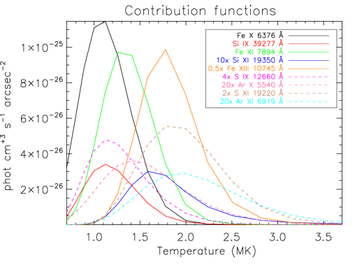
Figure 5.— Contribution functions of a few of the main lines formed around 1-2 MK, calculated with photospheric abundances. The full lines indicate ions from low-FIP elements, while the dashed line those from high-FIP elements. In a few cases, the values have been scaled as indicated.

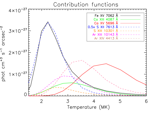
Figure 6.— Contribution functions of a few of the main lines formed around 2–5 MK, calculated with photospheric abundances. The full lines indicate ions from low-FIP elements, while the dashed line those from high-FIP elements. In a few cases, the values have been scaled as indicated.

Also in this case there are plenty of diagnostics, depending on which wavelength region is considered, and the source region. If one considers only the quiet Sun then most of the lines which are typically formed around 3 MK will not be observable, and the list of potentially interesting lines reduces significantly. Figure 5 shows the contribution functions of a few of the main lines formed around 1-2 MK (without photoexcitation included), calculated with photospheric abundances. Within the visible, excellent diagnostics are available with Ar x and Ar xi, when observed in conjunction with e.g. Fe x, Fe xi, and Fe xiii. There are obviously many more lines from many other elements that will be observable by DKIST.

Many more diagnostics are available when active regions are observed, as it is clear from the list of lines in Table 2. In Figure 6 we show what we believe are the most important lines. The best combination of lines for a 2 MK plasma is the ratio of the two strong lines of S xii at 7612 Å and Fe xv at 7062 Å, both of which have been observed regularly at eclipses. The best diagnostic of all for the cores of active regions is the ratio of Ar xiii 10143 Å with the Ca xiii 4087 Å. Their contribution functions are not very large, but in the cores of active region the emission measure at 3 MK is at least one or two orders of magnitude higher than the value at 1 MK, so these lines will become very strong. Indeed the Ca xiii has been observed to be strong (for a discussion of the Ca lines in the 1952 observation see Mason, 1975b). On the other hand, the Ar xiii 10143 Å has not been observed yet as far as we are aware. Other important lines are those from S xiii, Ar xiv at 4413 Å and potentially the Ar xv line if confirmed. Several interesting possibilities are also shown in Table 2. There are many transitions from K, Cl, Co, Mn that could potentially allow abundance measurements in the future, if the lines will be observed and accurate atomic data become available.

5.3. The near infrared

As already discussed, the near-infrared is basically an unexplored spectral region, with the exception of the few measurements we have cited. It remains to be seen which spectral lines are observable. According to our simulations, a number of weaker lines should be observable in the quiet Sun. Many of them were already pointed out by Judge (1998), but several were not. We predict that, for example, the Fe xii 2.2 $\mu$m should be among the strongest lines. The Al ix at 2.2 $\mu$m should also be stronger than many other lines in this spectral region. On the other hand, we predict very low signal in the transition-region lines such as Mg viii, Si vii, unless an active region is observed, or cooler material is present along the line of sight.

The intensities of the strong Si x 1.43 $\mu$m reported by Münch et al. (1967) and Olsen et al. (1971) are in relatively good agreement with our predicted radiances, while the S ix 1.26 $\mu$m reported by Olsen et al. (1971) is much stronger than any of our predictions. We know that the atomic model for S ix needs improvement, and that on the basis of our large-scale calculations we expect an increase by a factor of 2–3, but that might not seem sufficient to explain the observed intensity of this line. Regarding the other upper limits listed by Olsen et al. (1971), they are compatible with our rough estimates.

On a side note, we point out that several strong lines from H and He are predicted to be visible, and indeed have been reported by Olsen et al. (1971).

As shown in Figure 4, the S xi ratio is one of the best available across the whole visible/infrared spectrum, considering that it is not much affected by photoexcitation, and lines are relatively close in wavelength. We expect these lines to be visible.

As Figure 5 shows, excellent diagnostics for the FIP effect are available with S ix 1.26 $\mu$m and S xi 1.92 $\mu$m, in combination with e.g. observations of the Si ix 3.93 $\mu$m and Si xi 1.93 $\mu$m. We note that three of these lines are in the Air-Spec spectral range, and appear to have been successfully observed in the 2017 eclipse.

5.4. A few notes about DKIST CryoNIRSP

In its current design, the CryoNIRSP will produce routine measurements in a number of spectral bandpasses of about 20 Å in the visible and 100 Å in the infrared (see Fehlmann et al., 2016, for details). In terms of coronal lines, the instrument will observe the following lines: Fe xiv 5304 Å and the Fe xiii doublet of infrared lines at 10750, 10801 Å, plus several lines in the near-infrared, such as the S ix at 1.25 $\mu$m, Si x 1.43 $\mu$m, the still unobserved Fe ix and Si ix at 2.22 and 2.58 $\mu$m respectively, the Mg viii at 3.03 $\mu$m, and finally the still unobserved Si ix at 3.93 $\mu$m.

The above selection of lines reflects the primary science goal of the DKIST coronal observations, to obtain magnetic field measurements. This set of lines has in fact an excellent coverage of the quiet Sun coronal emission around 1 MK. However, in principle the instrument is capable of providing ground-breaking results in various other areas.

For example, with its current settings, DKIST will not observe the hot 3 MK emission from active regions. As we have mentioned previously, there is evidence, at the highest spatial resolution (Hi-C and AIA, 0.2 and 1″), that the 3 MK emission is not co-spatial with the 1–2 MK emission and has fundamentally different characteristics (see, e.g. Warren et al., 2008; Del Zanna, 2013).

Considering the profound influence that active regions have on the overall restructuring and chemical composition of the lower corona, we strongly advise the addition of a few other channels where at least a couple of strong lines formed around 3 MK are observed. There are plenty of options, but well-known strong lines that have been observed are the Fe xv at 7062 Å, the Ca xiii 4087 Å, and the famous yellow coronal line, the Ca xv 5694 Å.

According to the model proposed by Del Zanna et al. (2011); Bradshaw et al. (2011), interchange reconnection between the 3 MK loops and the surrounding corona continuously takes place high in the corona. This process is in principle capable of injecting coronal plasma that was originally present in the closed 3 MK loops into the heliosphere. It is well known that this plasma has enriched low-FIP elements, so this is a possible way by which active regions enrich the low corona with low-FIP elements, as indeed has been observed in some instances with in-situ ACE measurements (Wang et al., 2009). According to the model, some of the so-called coronal outflows, i.e. region connected to strong magnetic polarities (sunspots and moss) are the signatures of outflows into the heliosphere. If this is the case, we need measurements of abundances, flows, densities, non-thermal widths of 3 MK plasma, since these outflows are only seen in lines formed around 2–3 MK, as shown by Del Zanna (2008) and later confirmed by various authors (see, e.g. Warren et al., 2011).

To confirm this scenario, and in view of potentially important synergies with the in-situ close-by observations from the Parker’s Solar probe, and the in-situ plus remote-sensing measurements with the suite of instruments aboard Solar Orbiter, it is of paramount importance to add to the DKIST CryoNIRSP the capability to measure abundances of 3 MK plasma. Tracing the variations of the chemical composition from the low-corona to the solar wind is an important science goal of Solar Orbiter, and DKIST could provide invaluable information.

As briefly discussed in the previous section, the best combination of lines to measure the FIP effect are the Ar xiii 10143 Å with the Ca xiii 4087 Å, together with the S xiii, Ar xiv, if observed in combination to other lines from low-FIP elements. There is substantial evidence (see, e.g. Del Zanna, 2013) that in the low-corona the sulfur abundance varies hand in hand with the argon abundance, in the cores of active regions. However, there are in-situ measurements where this does not occur. Observing both argon and sulphur lines will hopefully shed light into the physical reasons as to why this happens. See the Living Review by Laming (2015) for more details.

6. Summary and conclusions

The present benchmark study is very satisfying for the visible forbidden lines, in that all the strongest lines classified with an ‘A’ by Aly et al. (1962b) are now firmly identified, and the latest atomic data provide relatively good agreement with observations, considering the various uncertainties in the calibration of the spectra. For a few spectral lines, we have provided new identifications.

Regarding the lines in class ‘B’, most of them still await identifications and/or the calculation of atomic data. Strangely enough, a few of the lines classified with a ‘C’ have actually been observed in other eclipses and now have a firm identification. We have also provided several tentative new identifications.

In the infrared region of the spectrum, we were unable to provide any meaningful comparison, given the paucity of observations. However, all the lines that have been observed are firmly identified, and we have corrected a few inaccuracies in the literature. As already pointed out by Judge (1998), there are several coronal lines that should be observable in this spectral region. The advantage of observing in this region is the lower sky brightness and lower photospheric continuum emission. The challenge is the transparency of the atmosphere to infrared radiation.

We hope that we have provided enough evidence that the visible and infrared forbidden lines can be used in the near future to measure chemical abundance variations, electron temperatures and densities, alongside coronal magnetic field measurements, if there is enough signal in the polarisation measurements. There are exciting opportunities ahead, to finally resolve some among the many mysteries of the solar corona using the forbidden visible and infrared lines.

Regarding the atomic data, improvements in the energies and the atomic rates are needed for several ions. Some of them are in progress, but a significant amount of work still needs to be carried out before all the lines can reliably be used for diagnostic purposes. The issue of laboratory spectroscopy for astrophysics is often overlooked by the funding bodies, and indeed the lack of reliable atomic data across the visible and infrared spectrum is no surprise.

The present rough guide relied on the atomic data available within CHIANTI version 8 (Del Zanna et al., 2015). The accuracy in the atomic data across the entire wavelength range considered here varies considerably, and further improvements are needed, as discussed in the Appendix. During the present study, we have highlighted several ions where no atomic data are yet available, an issue that we will address in the near future. Further discussions on specific ions of particular diagnostic interest are left for a future paper.

Appendix A A few notes about the atomic data

The present assessment would not have been possible without the accurate atomic cross sections for electron impact excitation recently produced by the UK APAP network for the iron and nickel ions: Fe viii: Del Zanna & Badnell (2014); Fe ix: Del Zanna et al. (2014); Fe x: Del Zanna et al. (2012a); Fe xi: Del Zanna & Storey (2013); Fe xii: Del Zanna et al. (2012b); Fe xiii: Del Zanna & Storey (2012); Fe xiv: Liang et al. (2010); Ni xi: Del Zanna et al. (2014); Ni xii: Del Zanna & Badnell (2016); Ni xv: Del Zanna et al. (2014). For each of these ions extensive benchmarks have been carried out, so the emissivities of the strongest lines should be reliable to within say a 10-30%, depending on the line. Within the CHIANTI version 8 database, such level of accuracy is not present for most of the other ions in the visible and infrared. However, for most the lines of interest, the present atomic data should be accurate enough for the present rough guide.

For Fe xv the calculations of Berrington et al. (2005) have a similar level of accuracy, while for the Ni xiii and Ni xvi, the calculations of Bhatia & Doschek (1998) and Bhatia & Doschek (1999) will need some improvement.

Considering the magnesium, sulphur, and silicon ions, the cross sections for the B-like Mg viii, S xii, and Si x calculated by Liang et al. (2012) should be accurate, while those for the other ions need improvement, because of the limited calculations (Si ix, S ix by Bhatia & Landi 2003) or because data were interpolated (S xi and S xiii).

Considering the calcium and argon ions, the cross sections for the F-like Ca xii and Ar x calculated by Witthoeft et al. (2007) should be relatively accurate, while those for the O-like Ca xiii and Ar xi by Landi & Bhatia (2005) and Landi & Bhatia (2006) should be improved. The cross-sections for C-like Ca xv calculated by Aggarwal et al. (1991) should be relatively accurate, while those of Ar xiii (Dere et al., 1979) need improvement. The data for the B-like Ar xiv calculated by Liang et al. (2012) should be accurate.

The atomic data for some of the above ions have been calculated and will be made available with the next version of CHIANTI. We also note that the UK APAP network will be carrying out new large-scale calculations for the C-, N-, and O-like isoelectronic sequences, where the current atomic data are not consistently accurate. This will improve considerably the atomic data for several ions considered in the present paper.

References

- Aggarwal et al. (1991) Aggarwal, K. M., Berrington, K. A., & Keenan, F. P. 1991, ApJS, 77, 441
- Aly et al. (1962a) Aly, M. K., Evans, J. W., & Orrall, F. Q. 1962a, ApJ, 136, 956
- Aly et al. (1962b) Aly, M. K. A. M. K., Evans, J. W., & Orrall, F. Q. 1962b, Sac Peak Observatory monograph
- Andretta et al. (2012) Andretta, V., Telloni, D., & Del Zanna, G. 2012, Sol. Phys., 279, 53
- Arnaud & Newkirk (1987) Arnaud, J., & Newkirk, G., Jr. 1987, A&A, 178, 263
- Asplund et al. (2009) Asplund, M., Grevesse, N., Sauval, A. J., & Scott, P. 2009, ARA&A, 47, 481
- Berrington et al. (2005) Berrington, K. A., Ballance, C. P., Griffin, D. C., & Badnell, N. R. 2005, Journal of Physics B Atomic Molecular Physics, 38, 1667
- Bhatia & Doschek (1998) Bhatia, A. K., & Doschek, G. A. 1998, Atomic Data and Nuclear Data Tables, 68, 49
- Bhatia & Doschek (1999) Bhatia, A. K., & Doschek, G. A. 1999, Atomic Data and Nuclear Data Tables, 71, 69
- Bhatia & Landi (2003) Bhatia, A. K., & Landi, E. 2003, Atomic Data and Nuclear Data Tables, 85, 169
- Bradshaw et al. (2011) Bradshaw, S. J., Aulanier, G., & Del Zanna, G. 2011, ApJ, 743, 66
- Byard & Kissell (1971) Byard, P. L., & Kissell, K. E. 1971, Sol. Phys., 21, 351
- Curtis et al. (1965) Curtis, G. W., Dunn, R. B., & Orrall, F. Q. 1965, in 1965 Solar Eclipse Symposium, 137
- Del Zanna (1999) Del Zanna, G. 1999, Ph.D. thesis, Univ. of Central Lancashire, UK
- Del Zanna (2003) Del Zanna, G. 2003, A&A, 406, L5
- Del Zanna (2008) Del Zanna, G. 2008, A&A, 481, L49
- Del Zanna (2012a) Del Zanna, G. 2012a, A&A, 546, A97
- Del Zanna (2012b) Del Zanna, G. 2012b, A&A, 537, A38
- Del Zanna (2013) Del Zanna, G. 2013, A&A, 558, A73
- Del Zanna et al. (2011) Del Zanna, G., Aulanier, G., Klein, K.-L., & Török, T. 2011, A&A, 526, A137
- Del Zanna & Badnell (2014) Del Zanna, G., & Badnell, N. R. 2014, A&A, 570, A56
- Del Zanna & Badnell (2016) Del Zanna, G., & Badnell, N. R. 2016, A&A, 585, A118
- Del Zanna et al. (2004) Del Zanna, G., Berrington, K. A., & Mason, H. E. 2004, A&A, 422, 731
- Del Zanna et al. (2015) Del Zanna, G., Dere, K. P., Young, P. R., Landi, E., & Mason, H. E. 2015, A&A, 582, A56
- Del Zanna et al. (2002) Del Zanna, G., Landini, M., & Mason, H. E. 2002, A&A, 385, 968
- Del Zanna & Mason (2003) Del Zanna, G., & Mason, H. E. 2003, A&A, 406, 1089
- Del Zanna & Mason (2014) Del Zanna, G., & Mason, H. E. 2014, A&A, 565, A14
- Del Zanna & Storey (2012) Del Zanna, G., & Storey, P. J. 2012, A&A, 543, A144
- Del Zanna & Storey (2013) Del Zanna, G., & Storey, P. J. 2013, A&A, 549, A42
- Del Zanna et al. (2014) Del Zanna, G., Storey, P. J., & Badnell, N. R. 2014, A&A, 566, A123
- Del Zanna et al. (2012a) Del Zanna, G., Storey, P. J., Badnell, N. R., & Mason, H. E. 2012a, A&A, 541, A90
- Del Zanna et al. (2012b) Del Zanna, G., Storey, P. J., Badnell, N. R., & Mason, H. E. 2012b, A&A, 543, A139
- Del Zanna et al. (2014) Del Zanna, G., Storey, P. J., Badnell, N. R., & Mason, H. E. 2014, A&A, 565, A77
- Del Zanna et al. (2014) Del Zanna, G., Storey, P. J., & Mason, H. E. 2014, A&A, 567, A18
- DeLuca et al. (2016) DeLuca, E., Samra, J., Golub, L., & Cheimets, P. 2016, AGU Fall Meeting Abstracts
- Dere et al. (1997) Dere, K. P., Landi, E., Mason, H. E., Monsignori Fossi, B. C., & Young, P. R. 1997, A&AS, 125, 149
- Dere et al. (1979) Dere, K. P., Widing, K. G., Mason, H. E., & Bhatia, A. K. 1979, ApJS, 40, 341
- Divan & Pecker (1960) Divan, L., & Pecker, C. 1960, Annales d’Astrophysique, 23, 541
- Dudík et al. (2014) Dudík, J., Del Zanna, G., Mason, H. E., & Dzifčáková, E. 2014, A&A, 570, A124
- Dudík et al. (2015) Dudík, J., et al. 2015, ApJ, 807, 123
- Dunn (1966) Dunn, R. B. 1966, ISA Transactions, 5, 119
- Edlén (1966) Edlén, B. 1966, Metrologia, 2, 71
- Edlén (1943) Edlén, B. 1943, ZAp, 22, 30
- Eissner & Seaton (1972) Eissner, W., & Seaton, M. J. 1972, Journal of Physics B Atomic Molecular Physics, 5, 2187
- Fawcett et al. (1972) Fawcett, B. C., Kononov, E. Y., Hayes, R. W., & Cowan, R. D. 1972, Journal of Physics B Atomic Molecular Physics, 5, 1255
- Fehlmann et al. (2016) Fehlmann, A., et al. 2016, in Proc. SPIE, Vol. 9908, Ground-based and Airborne Instrumentation for Astronomy VI, 99084D
- Feldman et al. (1997) Feldman, U., Behring, W. E., Curdt, W., Schuehle, U., Wilhelm, K., Lemaire, P., & Moran, T. M. 1997, ApJS, 113, 195
- Firor & Zirin (1962) Firor, J., & Zirin, H. 1962, ApJ, 135, 122
- Fisher & Pope (1971) Fisher, R., & Pope, T. 1971, Sol. Phys., 20, 389
- Fludra et al. (1999) Fludra, A., Del Zanna, G., Alexander, D., & Bromage, B. J. I. 1999, J. Geophys. Res., 104, 9709
- Gibson et al. (1999) Gibson, S. E., Fludra, A., Bagenal, F., Biesecker, D., del Zanna, G., & Bromage, B. 1999, J. Geophys. Res., 104, 9691
- Grotrian (1939) Grotrian, W. 1939, Naturwissenschaften, 27, 214
- Habbal et al. (2010) Habbal, S. R., et al. 2010, ApJ, 708, 1650
- Habbal et al. (2011) Habbal, S. R., et al. 2011, ApJ, 734, 120
- Jefferies et al. (1969) Jefferies, J. T., Orrall, F. Q., & Zirker, J. B. 1969, in Liege International Astrophysical Colloquia, Vol. 15, Liege International Astrophysical Colloquia, ed. C. Arpigny, B. Edlén, & P. Swings, 235
- Jefferies et al. (1971) Jefferies, J. T., Orrall, F. Q., & Zirker, J. B. 1971, Sol. Phys., 16, 103
- Judge (1998) Judge, P. G. 1998, ApJ, 500, 1009
- Judge et al. (2013) Judge, P. G., Habbal, S., & Landi, E. 2013, Sol. Phys., 288, 467
- Judge et al. (2002) Judge, P. G., Tomczyk, S., Livingston, W. C., Keller, C. U., & Penn, M. J. 2002, ApJ, 576, L157
- Kastner (1993) Kastner, S. O. 1993, Sol. Phys., 143, 197
- Keil et al. (2003) Keil, S., Rimmele, T., Keller, C., & ATST Team. 2003, Astronomische Nachrichten, 324, 303
- Kernoa et al. (1965) Kernoa, A., Michard, R., & Servajean, R. 1965, Annales d’Astrophysique, 28, 716
- Koutchmy et al. (1974) Koutchmy, S., Bareau, C., & Stellmacher, G. 1974, Academie des Sciences Paris Comptes Rendus Serie B Sciences Physiques, 278, 873
- Kuhn et al. (1996) Kuhn, J. R., Penn, M. J., & Mann, I. 1996, ApJ, 456, L67
- Kurt (1962) Kurt, V. G. 1962, Soviet Ast., 6, 349
- Kurucz (2006) Kurucz, R. L. 2006, ArXiv Astrophysics e-prints
- Laming (2015) Laming, J. M. 2015, Living Reviews in Solar Physics, 12
- Landi & Bhatia (2005) Landi, E., & Bhatia, A. K. 2005, Atomic Data and Nuclear Data Tables, 90, 177
- Landi & Bhatia (2006) Landi, E., & Bhatia, A. K. 2006, Atomic Data and Nuclear Data Tables, 92, 305
- Landi & Feldman (2003) Landi, E., & Feldman, U. 2003, ApJ, 592, 607
- Landi et al. (2002) Landi, E., Feldman, U., & Dere, K. P. 2002, ApJS, 139, 281
- Landi et al. (2016) Landi, E., Habbal, S. R., & Tomczyk, S. 2016, Journal of Geophysical Research (Space Physics), 121, 8237
- Liang et al. (2010) Liang, G. Y., Badnell, N. R., Crespo López-Urrutia, J. R., Baumann, T. M., Del Zanna, G., Storey, P. J., Tawara, H., & Ullrich, J. 2010, ApJS, 190, 322
- Liang et al. (2012) Liang, G. Y., Badnell, N. R., & Zhao, G. 2012, A&A, 547, A87
- Liebenberg et al. (1975) Liebenberg, D. H., Bessey, R. J., & Watson, B. 1975, Sol. Phys., 44, 345
- Lyot (1939) Lyot, B. 1939, MNRAS, 99, 580
- Lyot & Aly (1955) Lyot, B., & Aly, M. K. A. M. K. 1955, ApJ, 122, 438
- Magnant-Crifo (1973) Magnant-Crifo, F. 1973, Sol. Phys., 31, 91
- Magnant-Crifo (1974) Magnant-Crifo, F. 1974, Sol. Phys., 39, 141
- Mason (1975a) Mason, H. E. 1975a, MNRAS, 170, 651
- Mason (1975b) Mason, H. E. 1975b, MNRAS, 171, 119
- Mason & Nussbaumer (1977) Mason, H. E., & Nussbaumer, H. 1977, A&A, 54, 547
- Mouradian (1997) Mouradian, Z. 1997, in NATO Advanced Science Institutes (ASI) Series C, Vol. 494, NATO Advanced Science Institutes (ASI) Series C, ed. Z. Mouradian & M. Stavinschi, 169
- Münch et al. (1967) Münch, G., Neugebauer, G., & McCammon, D. 1967, ApJ, 149, 681
- Nikolsky et al. (1971) Nikolsky, G. M., Gulyaev, R. A., & Nikolskaya, K. I. 1971, Sol. Phys., 21, 332
- Olsen et al. (1971) Olsen, K. H., Anderson, C. R., & Stewart, J. N. 1971, Sol. Phys., 21, 360
- Penn (2014) Penn, M. J. 2014, Living Reviews in Solar Physics, 11, 2
- Penn & Kuhn (1994) Penn, M. J., & Kuhn, J. R. 1994, ApJ, 434, 807
- Petrie & Menzel (1942) Petrie, W., & Menzel, D. H. 1942, ApJ, 96, 395
- Pottasch (1964) Pottasch, S. R. 1964, MNRAS, 128, 73
- Querfeld (1977) Querfeld, C. W. 1977, Reports of the Lund Observatory, 12, 109
- Rimmele et al. (2015) Rimmele, T., et al. 2015, IAU General Assembly, 22, 2255176
- Rosner et al. (1978) Rosner, R., Tucker, W. H., & Vaiana, G. S. 1978, ApJ, 220, 643
- Shajn (1948) Shajn, G. A. 1948, Izvestiya Ordena Trudovogo Krasnogo Znameni Krymskoj Astrofizicheskoj Observatorii, 3, 64
- Singh et al. (2004) Singh, J., Sakurai, T., Ichimoto, K., & Watanabe, T. 2004, ApJ, 617, L81
- Singh et al. (1982) Singh, J., Saxena, A. K., & Bappu, M. K. V. 1982, Journal of Astrophysics and Astronomy, 3, 249
- Smitt (1977) Smitt, R. 1977, Sol. Phys., 51, 113
- Strong (1978) Strong, K. 1978, Ph.D. thesis, University College London, UK
- Swings (1943) Swings, P. 1943, ApJ, 98, 116
- Thuillier et al. (2004) Thuillier, G., Floyd, L., Woods, T. N., Cebula, R., Hilsenrath, E., Hersé, M., & Labs, D. 2004, Advances in Space Research, 34, 256
- Tomczyk et al. (2008) Tomczyk, S., et al. 2008, Sol. Phys., 247, 411
- Tomczyk et al. (2016) Tomczyk, S., et al. 2016, Journal of Geophysical Research (Space Physics), 121, 7470
- Van de Hulst (1953) Van de Hulst, H. C. 1953, The sun., ed. G. P. Kuiper 268
- Vásquez et al. (2003) Vásquez, A. M., van Ballegooijen, A. A., & Raymond, J. C. 2003, ApJ, 598, 1361
- Wang et al. (2009) Wang, Y.-M., Ko, Y.-K., & Grappin, R. 2009, ApJ, 691, 760
- Warren & Brooks (2009) Warren, H. P., & Brooks, D. H. 2009, ApJ, 700, 762
- Warren et al. (2008) Warren, H. P., Ugarte-Urra, I., Doschek, G. A., Brooks, D. H., & Williams, D. R. 2008, ApJ, 686, L131
- Warren et al. (2011) Warren, H. P., Ugarte-Urra, I., Young, P. R., & Stenborg, G. 2011, ApJ, 727, 58
- Witthoeft et al. (2007) Witthoeft, M. C., Whiteford, A. D., & Badnell, N. R. 2007, Journal of Physics B Atomic Molecular Physics, 40, 2969
- Wlérick & Fehrenbach (1963) Wlérick, G., & Fehrenbach, C. 1963, in IAU Symposium, Vol. 16, The Solar Corona, ed. J. W. Evans, 199
- Woods et al. (2009) Woods, T. N., et al. 2009, Geophys. Res. Lett., 36, L01101
- Woolley & Allen (1948) Woolley, R. D. V. R., & Allen, C. W. 1948, MNRAS, 108, 292
- Young et al. (2003) Young, P. R., Del Zanna, G., Landi, E., Dere, K. P., Mason, H. E., & Landini, M. 2003, ApJS, 144, 135
- Zirin (1970) Zirin, H. 1970, Sol. Phys., 11, 497