Light vector and axial mesons effective couplings to constituent quarks

Abstract

Low energy effective couplings of baryons’ constituent quarks to light vector and axial mesons are derived by considering quark polarization for a dressed one gluon exchange quark interaction. The quark field is splitted into two components, one for background constituent quarks and another one for quark-antiquark states, light mesons and the scalar chiral condensate. By considering a large quark effective mass derivative expansion, several effective coupling constants are resolved as functions of the original model parameters and of components of the quark and gluon propagators. Besides the leading single vector meson-constituent quark gauge-type effective coupling, several two-vector and axial mesons-constituent quark couplings are also obtained in the next leading order. Among these, vector and axial mesons mixings induced by constituent quark currrents are found. Approximated and exact ratios between the effective coupling constants in the limit of very large quark effective mass and numerical estimates are exhibitted. Numerical results of the corresponding form factors and of the (strong) vector meson quadratic radius are also presented.

I Introduction

Light vector mesons play an important role in a broad range of energies in Hadron and Nuclear Physics. Besides the problems related to their structure, it is interesting to understand in detail the emergence of the phenomenological models describing their interactions with hadrons sakurai at different energy density scales by departing from the more fundamental QCD degrees of freedom. There are different conceptual frameworks to describe their dynamics such as in Massive Yang Mills, Hidden Gauge Approach and WCCWZ among others sakurai ; HLS ; birse ; meissner ; eLSM ; anti-sym ; arriola ; ER-1986 being several of them equivalent birse . Although it is highly desirable to formulate an Effective Field Theory (EFT) that incorporates explicitely their degrees of freedom some difficulties arise by trying to define the correct power counting rules in the framework of Chiral Perturbation theory PLB-fuchs-etal ; djukanovic-etal . The lightest vector mesons ( $\rho$ and $\omega$) are expected to be more relevant for the low and intermediary energies regimes, being that axial chiral partners eventually are included such as the $A_{1}$ for the $\rho$ meson and, less often, an axial partner of the $\omega$ has also been considered eLSM ; bloch-etal-a1b1 ; PDG . The light vector mesons effective couplings to nucleons present less ambiguities than the strict (chiral) vector mesons dynamics birse ; SU3-1 ; tensor-current being extremely relevant in the short range nucleon and nuclear potentials rho-omega ; nuc-med1 . In the framework of the constituent quark model lavelle-mcm ; georgi ; weinberg-2010 mesons couple directly to constituent quarks and the resulting coupling constants are proportional to the corresponding vector mesons-baryons coupling constants. From the criteria of dimensionality and simplicity meissner ; birse , the leading different rho-quark couplings can be expected to be: $g_{v}V_{\mu}^{i}(x)j_{i,v}^{\mu}(x)$ and $g_{T}F_{\mu\nu}^{i}(x)j_{i,T}^{\mu\nu}(x)$ where $F_{\mu\nu}^{i}(x)$ is the vector meson strength tensor. The first one is the minimal gauge coupling to the vector current sakurai ; SU3-1 and the second one a momentum dependent tensor coupling to a tensor current tensor-current . Besides that it is worth to mention vector mesons mixings are interesting effects associated to charge symmetry violation thomas and they are expected to occur further in the nuclear medium klingl . These effects are usually parameterized in terms of effective Lagrangian terms without more fundamental justification from first grounds. So it is interesting to search for mechanisms from the quark and gluon more fundamental dynamics that generate hadron and nuclear effective models. Instantons have been considered to describe several low energy quark effective interactions instantons and other mechanisms have also been envisaged EPJA-2016 ; PLB-2016 . Although it is possible to constraint the phenomenological couplings usually suitable for the hadron and nuclear dynamical models, it is highly desirable to obtain a QCD-based derivation of the mechanism according to which the vector-mesons - baryons interactions emerge. There are considerable difficulties to obtain the complete QCD effective action by integrating out gluons exactly from QCD chineses . However it is already interesting to understand the emergence of hadron interactions from a restricted part of the QCD effective action. Besides the dynamical calculation of the hadrons effective coupling constants it is also important to extract the whole momentum dependence of their interactions by means of form factors. Eventually the correct behavior of these effective couplings constants and form factors with nuclear density, temperature and other variables up to the chiral transition scales can be obtained nuc-med2 .

In this work light quark-antiquark vector and axial mesons couplings to (nucleons) constituent quarks are derived by considering a quark-quark interaction mediated by a dressed (non perturbative) gluon propagator. The non perturbative gluon propagator will be therefore an external input for the calculation and it will be required that it has strength enough to provide Dynamical Chiral Symmetry Breaking (DChSB). Besides that, this is a way of considering part of the non Abelian gluon dynamics. Therefore the quark interaction given in expression (1) is selected from the QCD effective action to be investigated with well known analytical methods. One loop quark polarization is calculated after a Fierz transformation to allow for the investigation of more complete flavor structure. By considering the background field method background the quark field is splitted into sea and background (constituent) quarks. Light mesons fields are introduced in the following by means of the the auxiliary field method ERV ; PRC1 ; holdom ; NJL . This procedure has been described in detail in Refs. EPJA-2016 ; PLB-2016 ; FLB-2017 ; PRD-2014 ; PRD-2016 and therefore in the present work it will not be described extensively. This approach has shown capable of providing for example a derivation of different constituent quark-pion effective couplings without and with electromagnetic couplings and the leading terms of chiral perturbation theory EPJA-2016 ; FLB-2017 corresponding to a whole effective field theory for low energy QCD weinberg-2010 . The work is organized as it follows. In the next Section, the Fierz transformation, the quark field splitting and the introduction of auxiliary meson fields are briefly reminded. In the following Section a derivative and large quark effective mass expansion of the sea quark determinant is performed. The leading and next leading terms for vector mesons couplings to quarks are exhibited by resolving effective coupling constants. These effective coupling constants are written in terms of parameters of the initial Lagrangian and of components of the quark and gluon propagators. Some exact and approximated ratios between effective coupling constants are also exhibited for very large quark effective mass and numerical estimates are also presented. Finally the momentum dependent form factors and a detailed investigation of the strong vector and axial mesons quadratic radia are presented. A Summary is presented in the last Section.

II Flavor structure and auxiliary fields

The dressed one gluon exchange between quarks can be written as ERV ; PRC1 :

$$Z=N\int{\cal D}[\bar{\psi},\psi]\exp\;i\int_{x}\left[\bar{\psi}\left(i\not{\partial}-m\right)\psi-\frac{g^{2}}{2}\int_{y}j_{\mu}^{b}(x){\tilde{R}}^{\mu\nu}_{bc}(x-y)j_{\nu}^{c}(y)+\bar{\psi}J+J^{*}\psi\right]$$ (1)

Where the color quark current is $j^{\mu}_{a}=\bar{\psi}\lambda_{a}\gamma^{\mu}\psi$, $\int_{x}$ stands for $\int d^{4}x$, $i,j,k=0,...(N_{f}^{2}-1)$ will be used for SU(2) flavor indices and $a,b...=1,...(N_{c}^{2}-1)$ stands for color in the adjoint representation. The sums in color, flavor and Dirac indices are implicit. To account for the non-Abelian structure of the gluon sector the gluon propagator $\tilde{R}^{\mu\nu}_{bc}(x-y)$ must be non perturbative and, as an external input for the model, it will be required to have enough strength to yield Dynamical Chiral Symmetry Breaking (DChSB) with a given strength of the quark-gluon coupling. DChSB has been found in several works with different approaches, though somewhat similar, SD-rainbow ; SDE ; kondo ; cornwall . Other terms from QCD effective action, such as multiquark interactions eventually due the non Abelian gluon structure, are not considered. The aim of this work is therefore to investigate the resulting hadron effective interactions that are obtained by considering well known analytical methods presented below for the quark interaction (1). In several Landau type gauges the gluon propagator $\tilde{R}^{\mu\nu}_{ab}(k)$ can be written as:

$$\tilde{R}^{\mu\nu}_{ab}(k)=\delta_{ab}\left[\left(g^{\mu\nu}-\frac{k^{\mu}k^{\nu}}{k^{2}}\right)R_{T}(k)+\frac{k^{\mu}k^{\nu}}{k^{2}}R_{L}(k)\right],$$ (2)

where $R_{T}(k),R_{L}(k)$ are transversal and longitudinal components. By performing a Fierz transformation NJL the flavor structure of the interaction (1) can be exploited further by introducing the corresponding light quark-antiquark states and corresponding auxiliary fields for light mesons as it is usually done for the model (1) and NJL-type models. This Fierz transformed interaction will be written in terms of the bilocal flavor-quark currents built with the Dirac gamma matrices and the flavor SU(2) Pauli matrices. They are given by: $j_{s}(x,y)=\bar{\psi}(x)\psi(y)$, $j_{p}(x,y)=\bar{\psi}(x)i\gamma_{5}\sigma_{i}\psi(y)$, $j_{si}(x,y)=\bar{\psi}(x)\sigma_{i}\psi(y)$, $j_{ps}(x,y)=\bar{\psi}(x)i\gamma_{5}\psi(y)$, $j_{V}^{\mu}(x,y)=\bar{\psi}(x)\gamma^{\mu}\sigma_{i}\psi(y)$, $j_{A}^{\mu}(x,y)=\bar{\psi}(x)i\gamma_{5}\gamma^{\mu}\sigma_{i}\psi(y)$, $j_{vs}^{\mu}(x,y)=\bar{\psi}(x)\gamma^{\mu}\psi(y)$ and $j_{as}^{\mu}(x,y)=\bar{\psi}(x)i\gamma_{5}\gamma^{\mu}\psi(y)$. The complete resulting set of color singlet non local interactions are the following:

$$\frac{\Omega}{\alpha g^{2}} \equiv \left[j_{s}(x,y)j_{s}(y,x)+j_{p}^{i}(x,y)j_{p}^{i}(y,x)+j_{s}^{i}(x,y)j_{s}^{i}(y,x)\right.$$ (3)

$$+ \left.j_{p}(x,y)j_{p}(y,x)\right]R(x-y)-\frac{1}{2}\left[j_{\mu}^{i}(x,y)j_{\nu}^{i}(y,x)+{j_{\mu}^{i}}_{A}(x,y){j_{\nu}^{i}}_{A}(y,x)\right.$$

$$+ \left.j_{\mu}(x,y)j_{\nu}(y,x)+j_{\mu}^{A}(x,y)j_{\nu}^{A}(y,x)\right]\bar{R}^{\mu\nu}(x-y),$$

where $\alpha=4/9$ for flavor SU(2), and the following kernels were defined:

$$R{(x-y)} = 3R_{T}(x-y)+R_{L}(x-y),$$ (4)

$$\bar{R}^{\mu\nu}{(x-y)} = g^{\mu\nu}(R_{T}(x-y)+R_{L}(x-y))+2\frac{\partial^{\mu}\partial^{\nu}}{\partial^{2}}(R_{T}(x-y)-R_{L}(x-y)).$$

The background field method (BFM) background ; SWbook is applied next by splitting the quark field into sea quark, $\psi_{2}$, composing light quark-antiquark states and therefore light mesons and the chiral condensate, and the background (constituent) quark, $\psi_{1}$, eventually forming baryons. At the one loop level it is enough to perform quark bilinears shift background for each of the channel $m=s,p,si,pi,ps,V,A,as,vs$ defined with the currents above:

$$j^{m}=\bar{\psi}\Gamma^{m}\psi\to(\bar{\psi}\Gamma^{m}\psi)_{2}+(\bar{\psi}\Gamma^{m}\psi)_{1}.$$ (5)

This separation preserves chiral symmetry, and it may not correspond to a simply mode separation of low and high energies which might be a too restrictive assumption. The ambiguity involved in this splitting was discussed with more details in Ref. EPJA-2016 and it is outside the scope of this work. The effective Fierz transformed interaction $\Omega$ is then rewritten as sum of the different quark components interactions as $\Omega=\Omega_{1}+\Omega_{2}+\Omega_{12}$, where $\Omega_{i}$ stands for each of the component and $\Omega_{12}$ for the interaction terms between $\psi_{1}$ and $\psi_{2}$. Instead to proceed by neglecting $\Omega_{2}$ according to the usual one loop BFM, the auxiliary field method is considered to make possible the functional integration of the sea quark field. Besides that, it allows for introducing light mesons fields. A set of bilocal auxiliary fields (a.f.) is introduced by means of unitary functional integrals multiplying the generating functional kleinert . Although this work is concerned only with the vector and axial mesons, all the a.f. will be introduced and, latter, some of them will be neglected. There is one bilocal a.f. associated to each of the quark currents, and they are the following: $S(x,y),P_{i}(x,y),S_{i}(x,y),P(x,y),V_{\mu}^{i}(x,y),V_{\mu}(x,y),\bar{A}_{\mu}^{i}(x,y)$ and $\bar{A}_{\mu}(x,y)$. This way, besides the rho and A₁ mesons, the isoscalar vector $\omega$ and an isoscalar axial $f_{1}$ PDG ; eLSM are also considered, besides a scalar iso-quartet ($S_{i}$ and $P$) that will be taken into account elsewhere. The (unity Jacobian) shifts in the functional integrals also generate couplings to sea quarks. The bilocal auxiliary fields give origin to punctual meson fields by expanding in an infinite basis of local meson fields PRC1 , for instance a particular bilocal field the vector $V_{\mu}^{i}(x,y)$ can be writtten in terms of a corresponding complete orhonormal sum of local fields as:

$$V^{\mu}_{i}(x,y)=V^{\mu}_{i}\left(\frac{x+y}{2},x-y\right)=V^{\mu}_{i}(u,z)=\sum_{k}F_{k}(z)V^{\mu}_{i,k}(u),$$ (6)

where $F_{k}$ are vacuum functions invariant under translation for each of the local field $V^{\mu}_{i,k}(u)$. For the low energy regime one might pick up only the lowest energy modes, lighest $k=0$ and making the form factors to reduce to constants in the zero momentum limit $F_{k}(z)=F_{k}(0)$. In the case of expression (6) this mode turns out to be structureless isotriplet local mesons $V^{\mu}_{i,k=0}(u)=\rho^{\mu}_{i}(x)$. From here on, these structureless lowest modes for each of the channels will be denoted by: $S(x),P_{i}(x),S_{i}(x),P(x),V_{\mu}^{i}(x),V_{\mu}(x),\bar{A}_{\mu}^{i}(x),\bar{A}_{\mu}(x)$. In the present work only the vector and axial mesons couplings to constituent quarks will be addressed. Pions and the other eventual scalar or pseudoscalar quark-antiquark states have been considered elsewhere and will be neglected, except for the fact that the scalar field can give rise to a constant contribution in the vacuum. The resulting structureless vector and axial mesons local couplings to quarks, by omitting the index ₂, can be written as:

$$\bar{\psi}(x)\Xi_{v}(x-y)\psi(y)=\bar{\psi}(x)\tilde{\Xi}_{v}(x)\delta(x-y)\psi(y) = -\bar{\psi}(x)\frac{\gamma^{\mu}}{2}\left[F_{v}\sigma_{i}\left(V_{\mu}^{i}(x)+i\gamma_{5}\bar{A}_{\mu}^{i}(x)\right)\right.$$ (7)

$$+ \left.F_{vs}\left(V_{\mu}(x)+i\gamma_{5}\bar{A}_{\mu}(x)\right)\right]\psi(x)\delta(x-y),$$

where the constants $F_{v}$ and $F_{vs}$ provide the canonical field definition respectively of rho and A₁ mesons and of $\omega$ and axial $f_{1}$.

The Gaussian integration of the sea quark field can now be performed and, by making use of the identity $\det A=\exp\;Tr\;\ln(A)$, it yields:

$$S_{eff} = Tr\;\ln\;\left\{-i\left[{S_{0}}^{-1}(x-y)+\Xi_{v}(x-y)+\sum_{q}a_{q}\Gamma_{q}j_{q}(x,y)\right]\right\}$$ (8)

where $Tr$ stands for traces of all discrete internal indices and integration of spacetime coordinates, $Tr=\int d^{4}x\,tr_{D}\,tr_{C}\,tr_{F}$ with the traces in Dirac, color and flavor indices, where the free quark kernel can be written as $S_{0}^{-1}(x-y)=\left(i\not{\partial}-m\right)\delta(x-y)$ and the following notation was used for the constituent quark currents, by omitting the index ₁ since sea quarks have already been integrated out:

$$\frac{\sum_{q}a_{q}\Gamma_{q}j_{q}(x,y)}{\alpha g^{2}} = 2R(x-y)\left[\bar{\psi}(y)\psi(x)+i\gamma_{5}\sigma_{i}\bar{\psi}(y)i\gamma_{5}\sigma_{i}\psi(x)\right.$$ (9)

$$+ \left.\bar{\psi}(y)\sigma_{i}\psi(x)+i\gamma_{5}\bar{\psi}(y)i\gamma_{5}\psi(x)\right]$$

$$- \bar{R}^{\mu\nu}(x-y)\gamma_{\mu}\sigma_{i}\left[\bar{\psi}(y)\gamma_{\nu}\sigma_{i}\psi(x)+i\gamma_{5}\bar{\psi}(y)i\gamma_{5}\gamma_{\nu}\sigma_{i}\psi(x)\right]$$

$$- \bar{R}^{\mu\nu}(x-y)\gamma_{\mu}\left[\bar{\psi}(y)\gamma_{\nu}\psi(x)+i\gamma_{5}\bar{\psi}(y)i\gamma_{5}\gamma_{\nu}\psi(x)\right].$$

Expression (8) has already been investigated in different limits: for the complete pion sector by considering pion structure for example in PRC1 and structureless pions coupled to constituent quarks in the vacuum and coupled to the electromagnetic field EPJA-2016 ; FLB-2017 providing all the leading chirally symmetric and symmetry breaking terms of Chiral Perturbation Theory. In Refs. meissner ; ER-1986 the chiral vector mesons sector ($\rho$ and $A_{1}$), without quarks, was investigated at length. The purely constituent quark sector was investigated to derive higher order quark effective couplings, and magnetic field dependent effective interactions PLB-2016 ; PRD-2016 ; FLB-2017 .

The determination of the auxilary fields in the ground state makes possible to incorporate dynamical chiral symmetry breaking, as it is usually done for the NJL model and analogously for the Schwinger-Dyson approach. The saddle point equations for the a.f., by denoting each of them by $\phi_{\alpha}$, are given by: $\frac{\partial S_{eff}}{\partial\phi_{\alpha}}=0$. These equations for the NJL model and global color model have been analyzed in many works in the vacuum or under a finite energy density. The scalar a.f. is the only non trivially zero in the vacuum provided the strength of the gluon propagator and the quark gluon (running) coupling constant are strong enough for that. It corresponds to a scalar quark-antiquark condensate and it produces a large effective quark mass. A constant value for the solution of the scalar field gap equation yields a correction to the quark effective mass in expression (8). In this case the quark kernel above can then be written in terms of the quark effective mass $M^{*}$ as usually done EPJA-2016 ; PLB-2016 ; FLB-2017 and besides that it might incorporate the quark coupling to vector and axial mesons that might be seen as a covariant derivative, $\not{D}_{v}=\not{\partial}-i\;\tilde{\Xi}_{v}$. It can then be written as:

$$S_{v}^{-1}(x-y)=\left(i\not{\partial}-M^{*}\right)\delta(x-y)+\Xi_{v}(x-y).$$ (10)

III Large quark mass expansion and effective couplings

The quark determinant can be rewritten as:

$$I_{det} = \frac{i}{2}Tr\ln\left[\left(1+S_{v}(x-y)\sum_{q}a_{q}\Gamma_{q}j_{q}(y,x)\right)\right.$$ (11)

$$\left.\left(1+{S}_{v}(x-y)\left(\sum_{q}\bar{a}_{q}\Gamma_{q}j_{q}(y,x)\right)\right)^{*}\right]+I_{0},$$

where $I_{0}$ yields a multiplicative constant in the generating functional with corrections exclusively from the vector and axial mesons meissner which are outside the scope of this work.

Next, a large quark and gluon effective masses and zero order derivative expansion of the determinant is performed at the zero order derivative expansion mosel . Equivalently a weak vector/axial field and large gluon effective mass can be considered. The large gluon effective mass limit leads to a weak strength of the gluon propagator in expression (11) and consequently small effective coupling constants for the terms of the expansion with quark currents as shown below. The leading effective action interaction terms $I_{det}^{l.o.}$ for the effective constituent quark couplings to the canonically defined vector and axial mesons are presented now. As an example the vector meson $V_{\mu}^{i}$ interaction with constituent quark term is given by the following effective action term:

$$I_{det,V_{\mu}^{i}}^{l.o.}=\frac{i}{2}\;Tr\;\left(S_{0}(y-x)\frac{\gamma^{\mu}\sigma_{i}}{2}V_{\mu}^{i}(x)S_{0}(x-z)\bar{R}^{\rho\sigma}(y-z)\gamma_{\rho}\sigma_{j}\bar{\psi}(z)\gamma_{\sigma}\sigma_{j}\psi(y)\right).$$ (12)

With the insertion of complete sets of orthogonal momentum states, effective coupling constants, $g_{r1}$ and $g_{v1}$, are resolved in the local limit for zero momentum exchange and the term above can be written as $I_{det,V_{\mu}^{i}}^{l.o.}=\int d^{4}x\;g_{r1}V^{\mu}_{i}\bar{\psi}\gamma_{\mu}\sigma_{i}\psi$. In this limit the resulting four leading effective Lagrangian interaction terms can be written as:

$${\cal L}_{v-q}=g_{r1}\left(V^{\mu}_{i}(x)j^{V,i}_{\mu}(x)+\bar{A}^{\mu}_{i}(x)j^{A,i}_{\mu}(x)\right)+g_{v1}\left(V^{\mu}(x)j_{\mu}(x)+\bar{A}_{\mu}(x)j_{A}^{\mu}(x)\right)$$ (13)

where, by taking the traces in Dirac, color and isospin indices, the following effective dimensionless coupling constants were defined

$$g_{r1}=g_{v1} = 4iN_{c}d_{1}(\alpha g^{2})\;Tr^{\prime}\;(({S}_{0}(k)S_{0}(k)\bar{\bar{R}}(k))),$$ (14)

where $\bar{\bar{R}}(k)=\bar{R}^{\mu\nu}(k)\;g_{\mu\nu}$, $Tr^{\prime}$ stands for the integral in internal momentum of components of quark and gluon kernels for the limit of zero momentum exchange and $d_{n}=i\frac{(-1)^{n+1}}{2n}$. These couplings correspond to the minimal couplings proposed by Sakurai sakurai and extended for the chiral case with axial mesons. Differently from the nucleon level, the $\rho$-constituent quark and $\omega$-constituent quark coupling constants are equal without a factor $1/3$ for the rho coupling rho-omega . The corresponding Feynman diagrams are presented in Figure (1a) where the dashed line stands for any of the vector or axial mesons. The zero order derivative expansion is suitable for the local low energy regime and higher order derivative effective couplings of the type: $G_{dnVj}\partial^{n}V_{\mu}(x)j^{\mu}(x)$ for $n\geq 2$ are neglected.

Besides that, in the next leading order of the large quark mass expansion, there are three types of two-vector/axial -mesons constituent quark current couplings. The very longwavelength and zero momentum transfer limits, for the leading terms from the first order expansion, can be written, in terms of the canonically normalized mesons and by omitting the spacetime dependence of the fields and currents, as:

$${\cal L}_{2v-j} = g_{va-j}\left(\left[V_{\mu}\bar{A}^{\mu}_{i}+V_{\mu}^{i}\bar{A}^{\mu}\right]j_{ps}^{i}+\left[V_{\mu}^{i}\bar{A}^{\mu}_{i}+V_{\mu}\bar{A}^{\mu}\right]j_{ps}\right)$$ (15)

$$+ g_{va-j}\left(\left[(V_{\mu}^{2}+\bar{A}_{\mu}^{2})+({V_{\mu}^{i}}^{2}+(\bar{A}^{\mu}_{i})^{2})\right]j_{s}+\left[V^{\mu}V_{\mu}^{i}+\bar{A}_{\mu}\bar{A}^{\mu}_{i}\right]j_{s}^{i}\right)$$

$$+ g_{Fjs}\left[\left(({\cal F}_{\mu\nu}{\cal F}^{\mu\nu}+{\cal F}_{\mu\nu}^{A}{\cal F}^{\mu\nu}_{A})+({\cal F}_{\mu\nu}^{i}{\cal F}^{\mu\nu}_{i}+{\cal F}_{\mu\nu}^{A,i}{\cal F}^{\mu\nu}_{A,i})\right)j_{s}\right.$$

$$+ \left.\left({\cal F}_{\mu\nu}^{i}{\cal F}^{\mu\nu}_{A}+{\cal F}_{\mu\nu}{\cal F}^{\mu\nu}_{A,i}\right)j_{p}^{i}+\left({\cal F}_{\mu\nu}^{i}{\cal F}^{\mu\nu}+{\cal F}_{\mu\nu}^{A,i}{\cal F}^{\mu\nu}_{A}\right)j_{s}^{i}+\left({\cal F}_{\mu\nu}{\cal F}^{\mu\nu}_{A}+{\cal F}_{\mu\nu}{\cal F}^{\mu\nu}_{A}\right)j_{p}\right]$$

$$+ g_{\epsilon v}i\epsilon_{ijk}\left({\cal F}_{\mu\nu}^{i}V^{\nu}_{j}+{\cal F}^{i,A}_{\mu\nu}\bar{A}_{j}^{\nu}\right)j_{k,V}^{\mu}+g_{\epsilon v}i\epsilon_{ijk}\left({\cal F}_{\mu\nu}^{i}\bar{A}^{\nu}_{j}+{\cal F}^{i,A}_{\mu\nu}\bar{V}_{j}^{\nu}\right)j_{k,A}^{\mu}$$

where the Abelian tensors for each of the fields were defined as:

$${\cal F}^{i}_{\mu\nu} = \partial_{\mu}V_{\nu}^{i}-\partial_{\nu}V_{\mu}^{i},\;\;\;\;\;\;\;{\cal F}_{\mu\nu}=\partial_{\mu}V_{\nu}-\partial_{\nu}V_{\mu},$$ (16)

$${\cal G}^{i}_{\mu\nu} = \partial_{\mu}\bar{A}_{\nu}^{i}-\partial_{\nu}\bar{A}_{\mu}^{i},\;\;\;\;\;\;\;{\cal G}_{\mu\nu}=\partial_{\mu}\bar{A}_{\nu}-\partial_{\nu}\bar{A}_{\mu}.$$

In the expression (15) the following effective coupling constants have been defined for the zero momentum transfer limit:

$$g_{va-j} = i\;12N_{c}d_{2}(\alpha g^{2})\;Tr^{\prime}(({S}_{0}(k){S}_{0}(k){S}_{0}(k)R(k))),$$ (17)

$$g_{\epsilon v} = -\frac{g_{va-j}}{M^{*}},$$ (18)

$$g_{Fjs} = -i\;12N_{c}d_{2}(\alpha g^{2})\;Tr^{\prime}(({S}_{0}(k)\tilde{S}_{0}(k)\tilde{S}_{0}(k)R(k)\;)),$$ (19)

In these expressions the following function is used: $\tilde{S}_{0}(k)=\frac{1}{k^{2}-{M^{*}}^{2}}$, by implicitely assuming a regularization procedure. Interesting to note there are very few coupling constants for several different couplings along the lines of the Universality idea. Whereas the single vector/axial meson coupling to quark current is dimensionless, these couplings have the following dimensions: $g_{va-j}\sim M^{-1}$, $g_{\epsilon v}\sim M^{-2}$ and $g_{Fjs}\sim M^{-3}$ where $M$ is an energy scale. These effective coupling constants are the zero momentum exchange limit of the corresponding form factors and they are proportional to the elastic and inelastic scattering amplitudes. The inelastic case terms might also be seen as type of mixing mediated or induced by different quark currents. Among these effective coupling constants, $g_{Fjs}$ is one order of magnitude smaller than the others within the large quark mass $M^{*}$ expansion by a factor $\tilde{S}_{0}\sim 1/{M^{*}}^{2}$. Most of these couplings do not seem to be possibly incorporated into a chiral vector/axial mesons gauge framework meissner ; birse ; HLS in the sense that the couplings of the first line ($g_{va-j}$) and also from the last line ($g_{\epsilon v}$), such as $V_{\mu}\bar{A}^{\mu}_{i}j_{ps}^{i}$, cannot be written in terms of parts of non Abelian vector mesons tensors that generalize expressions (16). In progressively higher order terms of the determinant expansion, i.e. for more than two vector mesons involved or more than one constituent quark current, there are also higher order n -vector mesons-quark interactions being that each of the additional external vector/axial meson field has an extra factor $S_{0}(k)$ or $\tilde{S}_{0}$(k) that contributes to suppress the corresponding coupling constant by $1/M^{*}$ or $1/{M^{*}}^{2}$ in the large quark mass expansion. The strengths of the corresponding higher order vector/axial mesons couplings to constituent quarks are reduced considerably and progressively in the limit of large quark effective mass. Exactly the same behavior was noticed for higher order quark effective interactions PLB-2016 . At higher energies eventually close to the chiral restoration transition the large quark effective mass expansion might not be valid anymore and a different treatment of the determinant is required. Other types of quark currents might be considered to contribute to the structure of a vector meson such as: $j_{V_{1}}^{\mu}=\bar{\psi}i\partial^{\mu}\psi$ and $j_{T}^{\mu\nu}=\bar{\psi}\sigma^{\mu\nu}\psi$. Although the first of them might be obtained from the derivative expansion, their contributions for the vector mesons structure and their interactions with constituent quark interactions are outside the scope of this work.

The corresponding Feynman diagrams are presented in figure (1b) for the effective couplings with $g_{va-j}$; (1c) for the effective couplings of the types of $g_{\epsilon v}$ and in (1d) for the effective couplings of the type $g_{Fjs}$. The dashed lines stand for any of the vector/axial mesons and the dot-dashed lines for any of the tensors ${\cal F}_{\mu\nu},{\cal F}_{\mu\nu}^{i},{\cal G}_{\mu\nu},{\cal G}_{\mu\nu}^{i}$. The different thickness of the dashed and dot-dashed lines stand for the possibility of the couplings between different vector or axial mesons, i.e. in the case these diagrams can be seen as vector/axial mesons mixings due to the interaction with a constituent quark current.

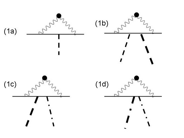
Figure 1: In these diagrams, the wavy line with a full dot is a (dressed) non perturbative gluon propagator, the solid line represents the constituent quark, the dashed line represents a vector or axial meson $V_{\mu},V_{\mu}^{i},\bar{A}_{\mu},\bar{A}_{\mu}^{i}$ and dot-dashed line represents a strength tensor line for a vector/axial meson ${\cal F}_{\mu\nu},{\cal F}^{i}_{\mu\nu},{\cal F}^{A}_{\mu\nu},{\cal F}^{i,A}_{\mu\nu}$. Diagram (1a) stands for the couplings $g_{r1}$ and $g_{v1}$. Diagrams (1b), (1c) and (1d) represent respectively effective couplings with coupling constants $g_{va-j}$, $g_{\epsilon v}$ and $g_{Fjs}$ from expression (15). In diagrams (1b,1c,1d) the vector or axial mesons lines might be the same or they might be different in the case of mixings, therefore the corresponding lines were drawn with different thickness.

III.1 Free vector and axial mesons terms

Although the aim of this work is to investigate vector/axial mesons interactions with constituent quarks it is interesting to have in mind some leading terms emerging from the effective action (11) for the strict vector/axial mesons sector. This sector has been investigated in some works within very similar formalisms for the NJL model meissner ; ER-1986 and expression (21) below contains basically the same vector mesons free terms. The following leading free vector/axial mesons terms arise in the very longwavelength limit for zero momentum exchange:

$$I_{free} = -\frac{g_{f}^{(0)}}{4}\left({\cal F}^{\mu\nu}_{i}{\cal F}_{\mu\nu}^{i}+{\cal G}^{\mu\nu}_{i}{\cal G}_{\mu\nu}^{i}+{\cal F}^{\mu\nu}{\cal F}_{\mu\nu}+{\cal G}^{\mu\nu}{\cal G}_{\mu\nu}\right)-\frac{M_{v}^{(0)}}{2}\left({V_{\mu}^{i}}^{2}+{\bar{A}_{i,\mu}}^{2}+{V_{\mu}}^{2}+{\bar{A}_{\mu}}^{2}\right),$$ (20)

where the following effective parameters have been defined:

$$g_{f}^{(0)} = id_{1}4N_{c}\;Tr^{\prime}\;((\tilde{S}_{0}(k)\tilde{S}_{0}(k))),$$ (21)

$${M_{v}^{(0)}}^{2} = -id_{1}8N_{c}\;Tr^{\prime}\;(({S}_{0}(k)S_{0}(k))).$$ (22)

It is interesting to note that both of the two quantities, $g_{f}$ and $M_{v}^{2}$, are the same for all the vector and axial mesons. They remain non zero in the chiral limit of zero quark effective mass $M^{*}\to 0$. In this formulation the vector/axial mesons masses are all the same for the four mesons (22) and the normalization constants of the canonical meson field definitions are also the same. Therefore these expressions only satisfy one of the Weinberg sum rules, $f_{V}^{2}m_{V}^{4}=f_{A}^{2}m_{A}^{4}$, due to the absence of the coupling to pions andrionov-espriou . The complete resulting vector and axial meson sector with leading self interactions will be presented elsewhere.

IV Numerical results

The expressions for the effective coupling constants depend on components of the gluon and quark propagator. However it is possible to find exact and approximated ratios between them that provide approximated estimations of their relative strengths. The limit of very large quark effective mass might be obtained, for example, by observing that $S_{0}(k)\sim 1/M^{*}$ and $\tilde{S}_{0}(k)\sim 1/{M^{*}}^{2}$. This yields the following approximated ratios:

$$\frac{g_{va-j}}{g_{r1}}\sim\frac{3}{2M^{*}}, \;\;\;\;\;\;\;\;\frac{g_{Fjs}}{g_{r1}}\sim\frac{3}{2{M^{*}}^{3}}.$$ (23)

These ratios show that the gauge-type single vector mesons couplings to quark currents $g_{r1}$ are the leading ones as compared to the others in the large quark mass expansion presented above as it should be. There is also an exact ratio between coupling constants that is given by:

$$\frac{g_{\epsilon v}}{g_{va-j}}=-\frac{1}{M^{*}}.$$ (24)

This exact ratio has the shape of a gauge invariant relation since it does not depend on the gluon propagator, however it has been found by considering (2).

In Table 1 numerical values are presented for the effective coupling constants of expressions (14,17,19) and also for the parameters (21,22) for different values of the quark effective mass. Two gluon propagators were chosen, one of them with only a transversal component from Tandy-Maris $D_{I}(k)$ SD-rainbow ; gluon-pro and the other is an effective longitudinal one by Cornwall $D_{II}(k)$ cornwall . Both of them are written below, they yield dynamical chiral symmetry breaking and the following association was adopted:

$$g^{2}\tilde{R}^{\mu\nu}(k)\equiv h_{a}D_{i}^{\mu\nu}(k)$$ (25)

where $D^{\mu\nu}_{i}(k)$ ($i=I,II$) is one of the chosen gluon propagators from the quoted articles, $h_{a}$ is a constant factor which corresponds to fix the quark gluon (running) coupling constant. The value of this factor $h_{a}$ was chosen to make the coupling constant $g_{v1}=g_{r1}$ to reproduce a typical numerical value considered in nucleon nucleon potential rho-omega in the vacuum or from nuclear properties. For example from the KSRF relation rho-omega ; SWbook ; djukanovic in the vacuum can be written as $g^{2}=\frac{M_{\rho}^{2}}{2F_{\pi}^{2}}$, where $M_{\rho}=770$ MeV and $F_{\pi}=92$ MeV, it yields $g\simeq 6$. From quark meson coupling model in different approximations these in medium coupling constants have values in a range $4.2\leq g_{\rho}\leq 8.5$ and $6.8\leq g_{\omega}\leq 9.5$ qmc-coupling . The fixed chosen value was $g_{v1}h_{a}=12$. The overall normalization and momentum dependence of the gluon propagators are different and therefore they provide considerably different values for the resulting vector mesons-constituent quark coupling constants. The expressions for the gluon propagators considered below are the following:

$$D_{I}(k) = \frac{8\pi^{2}}{\omega^{4}}De^{-k^{2}/\omega^{2}}+\frac{8\pi^{2}\gamma_{m}E(k^{2})}{\ln\left[\tau+(1+k^{2}/\Lambda^{2}_{QCD})^{2}\right]},$$ (26)

$$D_{II}(k) = K_{F}/(k^{2}+M_{k}^{2})^{2},$$ (27)

where for the first expression $\gamma_{m}=12/(33-2N_{f})$, $N_{f}=4$, $\Lambda_{QCD}=0.234$GeV, $\tau=e^{2}-1$, $E(k^{2})=[1-exp(-k^{2}/[4m_{t}^{2}])/k^{2}$, $m_{t}=0.5GeV$, $\omega=0.5$GeV, $D=0.55^{3}/\omega$ (GeV²) SD-rainbow ; gluon-pro ; and for the second expression $K_{F}=(2\pi M_{k}/(3k_{e}))^{2}$ where $k_{e}=0.15$ was chosen together with the value of $h_{a}$ and $M_{k}=220$MeV cornwall . The numerical results for the free vector mesons parameters $g_{f}^{(0)}$ and $M_{v}^{(0)}$ are ultraviolet (UV) divergent and therefore a momentum cutoff was considered. However these two parameters cannot be expected to reproduce experimental data due to the limit of structureless mesons considered in this work. When comparing the numerical values exhibitted in the Table it is seen they do not satisfy the ratios estimated above (23,24) because the effective quark mass $M^{*}\sim 330$MeV is not large enough to reproduce the analytical ratios above. Larger values of the effective mass however are not realistic and they were not included in the Table. Nevertheless it can be noted that the resulting numerical values for larger values quark effective mass in the Table are closer to the approximated ratios estimated above.

Table 1: In the first column the quark effective masses are displayed with the values of the factor $h_{a}$ that were chosen to fix the coupling constant $g_{v1}=g_{r1}=12$ as a typical numerical value considered in nucleon nucleon potential rho-omega . In the second column the gluon propagators are indicated: $D_{I}(k)$ and $D_{II}(k)$ are the gluon propagators respectively from Refs. SD-rainbow ; gluon-pro and Ref. cornwall . In the other columns, results, that depend on the gluon propagator, from the expressions (14,17,19) are displayed and also parameters do not depend on the gluon propagator (21) and (22). The momentum cutoff used for the integrations (21,22) is indicated together with $g_{f}^{(0)}$.

$M^{*}$ , $h_{a}$	$D_{i}(k)$	$g_{r1}h_{a}$	$g_{vaj}h_{a}$	$g_{Fjs}h_{a}$	$g_{f}^{(0)}$ ($\Lambda$)	$M_{v}^{(0)}$
(GeV), -			(GeV-1)	(GeV-3)	- (GeV)	(GeV)
0.33, $\frac{12}{9.3}$	$D_{I}$	12	5.8	111	0.10 (2.0)	0.479
0.33, $\frac{12}{0.67}$	$D_{II}$	12	5.7	107	-	-
0.28, $\frac{12}{10.5}$	$D_{I}$	12	6.4	165	0.11 (2.0)	0.495
0.28, $\frac{12}{0.75}$	$D_{II}$	12	6.4	163	-	-
0.22, $\frac{12}{12.7}$	$D_{I}$	12	6.8	279	0.13 (2.0)	0.512
0.22, $\frac{12}{0.9}$	$D_{II}$	12	6.7	285	-	-
0.07, $\frac{12}{20.3}$	$D_{I}$	12	7.2	4944	0.22 (2.0)	0.545
0.07, $\frac{12}{1.5}$	$D_{II}$	12	7.6	3228	-	-

IV.1 Form factors

The complete expressions for two of the form factors $g_{r1}$ and $g_{va-j}$, expressions (14) and (17), will be generalized for non zero momentum transfer. To explain the notation, two examples of full momentum dependent terms in expressions (13) and (15) are shown corresponding to a particular channel of the diagrams shown in Fig. 1. They can be written after a Fourier transformation as:

$${\cal L}_{ff}=g_{r1}(Q)V_{\mu}^{i}(Q)\bar{\psi}(Q)\gamma^{\mu}\sigma^{i}\psi(0)+g_{va-j}(Q_{1},Q_{2})V_{\mu}^{i}(Q_{1})V^{\mu}(Q_{2})\bar{\psi}(Q_{1}+Q_{2})\sigma^{i}\psi(0).$$ (28)

The couplings $g_{va-j}$ in expression (15) are the same for two identical vector/axial mesons couplings to quarks and for two different vector/axial mesons couplings to quarks although the quark currents might be different in each case. After a Wick rotation to the Euclidean momentum space, the form factors were calculated numerically. For the two-vector mesons couplings to constituent quarks two different calculations were performed, a complete one (^com) and a momentum-truncated one (^tr). The truncated expression is obtained by the following approximation: $S_{0}(k)\simeq M^{*}\tilde{S}_{0}(k)$. The following expressions were investigated numerically:

$$g_{r1}(Q) = \;4N_{c}\;d_{1}(\alpha g^{2}){M^{*}}^{2}\;\int_{k}\tilde{S}_{0}(k)\tilde{S}_{0}(k+Q)\bar{\bar{R}}(-k),$$ (29)

$$g_{va-j}^{com}(Q_{1},Q_{2}) = 12\;N_{c}\;d_{2}(\alpha g^{2}){M^{*}}\;\int_{k}T_{Q_{1},Q_{2}}(k)\tilde{S}_{0}(k)\tilde{S}_{0}(k+Q_{1})\tilde{S}_{0}(k+Q_{1}+Q_{2}){{R}}(-k),$$ (30)

$$g_{va-j}^{tr}(Q_{1},Q_{2}) = 12\;N_{c}\;d_{2}(\alpha g^{2}){M^{*}}^{3}\;\int_{k}\tilde{S}_{0}(k)\tilde{S}_{0}(k+Q_{1})\tilde{S}_{0}(k+Q_{1}+Q_{2}){R}(-k),$$ (31)

where $\int_{k}=\int d^{4}k/(2\pi)^{4}$, and the momentum dependent functions above are given by:

$$\tilde{S}_{0}(k) = \frac{1}{k^{2}+{M^{*}}^{2}},$$ (32)

$$\tilde{S}_{2}(k,k+Q) = \frac{k^{2}+k\cdot Q-{M}^{2}}{(k^{2}+{M^{*}}^{2})((k+Q)^{2}+{M^{*}}^{2})},$$ (33)

$$T_{Q_{1},Q_{2}}(k) = \left[3k^{2}+4k\cdot Q_{1}+2k\cdot Q_{2}+Q_{1}\cdot Q_{2}+Q_{1}^{2}-{M^{*}}^{2}\right],$$ (34)

and $\bar{\bar{R}}(k)$ was given after expression (14).

In Figures 2-7 the form factors $g_{va-j}^{com}(Q_{1},Q_{2}),g_{va-j}^{tr}(Q_{1},Q_{2})$ of expressions above are presented as functions of $Q_{1}$ for the two gluon propagators $D_{I},D_{II}$ and different external momenta $Q_{2}$ by considering $M^{*}=330$MeV. The cases for two incoming vector/axial mesons to the vertex in the same direction, $Q_{1}\cdot Q_{2}=|Q_{1}||Q_{2}|>0$, are presented with solid lines and the case for one incoming meson and another outgoing meson ($Q_{2}<0$ and $Q_{1}\cdot Q_{2}=|Q_{1}||Q_{2}|<0$) from the interaction vertex, in the same longitudinal direction, are presented with dashed lines in all these Figures. The thick lines correspond to the complete expressions (^com) and the thin lines to the truncated ones ^tr. Figures (2,4,6) are drawn with propagator $D_{I}(k)$ and Figures (3,5,7) are drawn with $D_{II}(k)$. In Figs. (2) and (3) it was considered $Q_{2}=\pm Q_{1}$, whereas in Figs. (4) and (5) $Q_{2}=\pm 2Q_{1}$ and finally in Figs. (6) and (7) $Q_{2}=\pm Q_{1}/2$. In all these figures it is seen that the more intrincated momentum structures of $g_{va-j}^{com}(Q_{1},Q_{2})$ produce a non monotonic behavior whereas the truncated expression yields a much faster decreasing behavior of the form factor with increasing $Q_{1}$. In all the figures, the numerical values for mesons with opposite momenta $Q_{2}<0$ are always larger than the parallell incoming mesons $Q_{2}>0$. The former, in all cases, go to zero considerably slower than the latter. For $Q_{2}=+\frac{a}{2}Q_{1}$ ($a=1,2$ and $4$ respectively in Figures (6,7), (2,3) and (4,5) ) the complete expressions exhibit quite different behaviors with low momentum when comparing the results from propagators $I$ and $II$. The complete expression with propagator $I$ (Figs. 2,4,6) in thick solid lines yields a local minimum for low momentum $Q_{1}$ that turns out to be always close to zero in the case of the results with propagator $II$. It is also noted that the propagator $II$ yields results that go to zero faster with $Q_{1}$ than the calculation with propagator $I$. For the behavior of $g_{va-j}^{com}(Q_{1},Q_{2})$ with negative $Q_{2}=-\frac{a}{2}Q_{1}$ ($a=1,2,4$ in the Figures), there is a maximum value of $g_{va-j}^{com}$ that occurs in larger values of $Q_{1}$ for smaller $a$ (or smaller $Q_{2}$). For example, by comparing the thick dashed lines in Figures 4 and 6, respectively for $Q_{2}=-2Q_{1}$ and $Q_{2}=-Q_{1}/2$, the maximum value appears to be respectively around $Q_{1}\simeq 400$MeV and $Q_{1}\simeq 650$MeV for propagator $I$.

Figure 2: By considering the gluon propagator I from Ref. SD-rainbow ; gluon-pro the expressions for $g_{va-j}^{com}(Q_{1},Q_{2}=+Q_{1})$ and $g_{va-j}^{com}(Q_{1},Q_{2}=-Q_{1})$ are plotted respectively in solid thick line and dashed thick line; $g_{va-j}^{tr}(Q_{1},Q_{2}=+Q_{1})$ and $g_{va-j}^{tr}(Q_{1},Q_{2}=-Q_{1})$ are plotted respectively in solid line and dashed line.

Figure 3: By considering the gluon propagator II from Ref. cornwall the expressions for $g_{va-j}^{com}(Q_{1},Q_{2}=+Q_{1})$ and $g_{va-j}^{com}(Q_{1},Q_{2}=-Q_{1})$ are plotted respectively in solid thick line and dashed thick line; $g_{va-j}^{tr}(Q_{1},Q_{2}=+Q_{1})$ and $g_{va-j}^{tr}(Q_{1},Q_{2}=-Q_{1})$ are plotted respectively in solid line and dashed line.

Figure 4: By considering the gluon propagator I from Ref. SD-rainbow ; gluon-pro the expressions for $g_{va-j}^{com}(Q_{1},Q_{2}=+2Q_{1})$ and $g_{va-j}^{com}(Q_{1},Q_{2}=-2Q_{1})$ are plotted respectively in solid thick line and dashed thick line; $g_{va-j}^{tr}(Q_{1},Q_{2}=+2Q_{1})$ and $g_{va-j}^{tr}(Q_{1},Q_{2}=-2Q_{1})$ are plotted respectively in solid line and dashed line.

Figure 5: By considering the gluon propagator II from Ref. cornwall the expressions for $g_{va-j}^{com}(Q_{1},Q_{2}=+2Q_{1})$ and $g_{va-j}^{com}(Q_{1},Q_{2}=-2Q_{1})$ are plotted respectively in solid thick line and dashed thick line; $g_{va-j}^{tr}(Q_{1},Q_{2}=+2Q_{1})$ and $g_{va-j}^{tr}(Q_{1},Q_{2}=-2Q_{1})$ are plotted respectively in solid line and dashed line.

Figure 6: By considering the gluon propagator I from Ref. SD-rainbow ; gluon-pro the expressions for $g_{va-j}^{com}(Q_{1},Q_{2}=+Q_{1}/2)$ and $g_{va-j}^{com}(Q_{1},Q_{2}=-Q_{1}/2)$ are plotted respectively in solid thick line and dashed thick line; $g_{va-j}^{tr}(Q_{1},Q_{2}=+Q_{1}/2)$ and $g_{va-j}^{tr}(Q_{1},Q_{2}=-Q_{1}/2)$ are plotted respectively in solid line and dashed line.

Figure 7: By considering the gluon propagator II from Ref. cornwall the expressions for $g_{va-j}^{com}(Q_{1},Q_{2}=+Q_{1}/2)$ and $g_{va-j}^{com}(Q_{1},Q_{2}=-Q_{1}/2)$ are plotted respectively in solid thick line and dashed thick line; $g_{va-j}^{tr}(Q_{1},Q_{2}=+Q_{1}/2)$ and $g_{va-j}^{tr}(Q_{1},Q_{2}=-Q_{1}/2)$ are plotted respectively in solid line and dashed line.

Figure 8: The strong vector meson form factor $g_{r1}(Q)$ given in expression (29) is presented for the two gluon propagators I SD-rainbow ; gluon-pro - solid lines - and II cornwall - dashed lines. The quark effective mass was considered $M^{*}=330$MeV for thick lines and $M^{*}=280$MeV for thin lines. The normalized vector meson-nucleon form factor from Ref. vec-nuc-craig-etal is also presented for further comparison with corresponding normalization with results of the two propagators above: $F_{1}^{\rho}(0)=9.2$ (propagator I, thick dotted line) and $F_{1}^{\rho}(0)=6.7$ (propagator II, circles).

In Figure 8 the form factor $g_{r1}(Q)$ is plotted for $M^{*}=330$MeV with gluon propagators $D_{I}$ and $D_{II}$ respectively in thick solid and dashed lines. By considering $M^{*}=280$MeV the same convention was adopted for thin solid and thin dashed lines. The results for $M^{*}=330$MeV are compared to the nucleon vector form factor fitted by a quadrupolar form Ref. vec-nuc-craig-etal from Faddeev equation in dotted line and circles. This fit is given by expression: $F_{1}^{\rho}(Q^{2})=\frac{F_{1}^{\rho}(0)}{\left(1+\frac{Q^{2}}{\Lambda_{1,\rho}^{2}}\right)^{3}}$, where $\Lambda_{1,\rho}=1.12$ GeV, and $F_{1}^{\rho}(0)=g_{\rho NN}$ is in the range $4.82-6.4$ in different works. To allow the comparison of the strict momentum dependence the value of $F_{1}^{V}(0)$ was taken to be the numerical zero momentum form factors obtained in this work. Therefore $F_{1}^{\rho}(0)=9.2$ (propagator I, thick dotted line) and $F_{1}^{\rho}(0)=6.7$ (propagator II, circles). The large-$Q$ behavior of $g_{r1}(Q)$ is dictated by the quark effective mass as it can be seen in the region of $Q=2$GeV.

The strong vector meson form factors yields the strong squared radius for the vector and axial mesons. With the expression (29) the following expression was calculated:

$$<r_{\rho}^{2}>_{s} = -\left.6\frac{dg_{r1}(Q)}{dQ^{2}}\right|_{Q=0}.$$ (35)

An exact relation between this strong squared radius (35) and the electromagnetic squared radius for the rho and omega vector mesons, $<r_{\rho}^{2}>_{E}$ (in expression (41) of Reference FLB-2017c ) and $<r_{\omega}^{2}>_{E}$ (both for zero magnetic field) follows and it is given by:

$$<r_{\rho}^{2}>_{s}=\frac{2}{e}<r_{\rho}^{2}>_{E},\;\;\;\;\;\;\;\;\;<r_{\omega}^{2}>_{s}=\frac{2}{3e}<r_{\omega}^{2}>_{E}.$$ (36)

The rho quadratic radius (35) is presented in Fig. 9 for the two gluon propagators respectively $D_{I}$ and $D_{II}$. Most of the numerical results are of the order of magnitude of the experimental data, $<r^{2}_{\rho}>_{exp}\simeq 0.28-0.56$fm² exp-rhoqm ; holo-krein-etal , except the numerical results obtained with the gluon propagator $D_{I}$ for which the values are divided by a factor 10 to keep the scale of the figure. These resuts manifest the strong dependence of the results on the strength of the quark-gluon coupling and on the overall momentum dependence of the gluon propagator.

Figure 9: By considering propagators I and II the vector meson strong quadratic radius is exhibitted as a function of the quark effective mass $M^{*}$. Results are shown with and without the factor $h_{a}$ explained in the Table: with thick solid and thick dashed lines with $D_{I}(k)$ and they are multiplied by $1/10$ to be kept in the scale of the Figure. The cases for gluon propagator propagator $D_{II}$ are represented in dotted and dot-dashed lines respectively with and without $h_{a}$.

V Summary and final remarks

To summarize, different effective couplings between vector/axial mesons and constituent quarks were presented. The effective coupling constants were obtained as the zero momentum limit of form factors and they were expressed in terms of the parameters of the original model and of components of the quark and gluon kernels. The vector and axial mesons fields were introduced by means of the auxiliary field method and the $\omega$ and $f_{1}$ vector and axial mesons were considered to be chiral partners. The structureless mesons limit was considered for the zero order derivative and large quark effective mass expansion. The leading vector mesons-constituent quark interactions are the minimal gauge couplings in expression (13). The determinant expansion given by expression (10) can be written in terms of a covariant derivative for the minimal coupling with vector/axial mesons. However most of the two vector/axial mesons effective couplings to constituent quarks (15) cannot be written in terms of non Abelian parts of vector mesons strength tensors that generalize expressions (16) and therefore do not seem to be possibly incorporated into a chiral vector/axial mesons gauge framework meissner ; birse ; HLS . Some next leading, or second order, effective couplings can be associated to a part of the elastic and inelastic scattering amplitude of vector mesons-constituent quarks scattering amplitude and some of the inelastic ones might be seen as vector or axial mesons mixings mediated or induced by constituent quark currents exhibited in expression (15). They present considerably different structures from the usual charge symmetry violation mixing. Also they emerge not only for the neutral $\rho^{0},A_{1}$ but also for the charged $\rho,A_{1}$-mesons coupled to quark currents such as $\vec{\rho}^{\mu}(\partial_{\mu}\omega_{\nu})\;\cdot\bar{\psi}\vec{\sigma}\gamma^{\nu}\psi$. It is interesting to note that only one effective coupling constant was found to emerge in the leading order in expressions (13), and only three different coupling constants at the second order in expression (15) in spite of the relatively large number of different effective couplings. This issue goes along the Universality idea. However these effective couplings do not represent all the possible effective couplings since tensor quark currents are not obtained from the method presented in this work. The resulting leading single meson couplings (13) are the only renormalizable effective couplings and the higher order ones, such as (15), are non renormalizable. All the coupling constants, however, are UV finite for usual large momentum behaviors of the gluon propagator such as $D(p)\sim 1/p^{s}$ for $s>2$. Furthermore each additional vector/axial meson that appear in higher orders terms of the large quark mass expansion will present progressively additional factors $S_{0}(k)\sim 1/M^{*}$ and these extra factors will make the higher order coefficients of the terms (effective coupling constants) of the expansion to be progressively smaller in the large quark mass regime. Numerical estimates were presented by considering two very different gluon propagators. Although the resulting order of magnitude of the leading vector mesons-constituent quark coupling constants, $g_{v1},g_{r1}$, nearly reproduced experimental or expected values, these coupling constant $g_{v1},g_{r1}$ were normalized to a typical value considered in the literature by fixing a particular value for the quark-gluon coupling constant. This was done by fixing $h_{a}$ as shown in the Table. The other coupling constants of the Table, for which we found no values in the literature, were corrected accordingly. Eventually, it might be that, by considering all the complementary mechanism(s) from QCD for the couplings shown above - if there are relevant corrections in different QCD mechanisms - the gauge independence should be expected to be recovered at the hadron and nuclear levels. Nevertheless, although the effective coupling constants shown above have different dimensions, it was possible to estimate approximated and exact ratios between them in the limit of large quark effective mass. The momentum dependences of two different form factors, $g_{r1}(Q)$ and $g_{vqa-j}(Q_{1},Q_{2})$, were addressed also by considering a momentum truncation for the coupling $g_{va-j}$ in expression (31). The momentum of the second vector/axial meson was chosen to assume the following values $Q_{2}=\pm\frac{a}{2}Q_{1}$ for $a=1,2,4$, i.e. its modulus to be smaller, equal or larger than $Q_{1}$. Finally the quark effective mass dependence of the strong rho (or omega) square radius was investigated for the two gluon propagators. Pions dynamics and effective couplings to constituent quarks were presented in Ref. EPJA-2016 and they make possible to consider constituent quark and vector mesons effective interactions mediated by them. They would correspond to a class of effective hadron interactions mediated by pseudoscalar auxiliary fields that can be found by integrating out them approximatedly. With this, the resulting effective couplings would contain additional factors $S_{0}(k)$ or $\tilde{S}_{0}(k)$ being thereore of higher order in $1/M^{*}$ and therfore numerically smaller.

References

- (1) J.J. Sakurai, Ann. of Phys. 11, 1 (1960).
- (2) M. Bando, T. Kugo, and K. Yamawaki, Phys. Rept. 164, 217 (1988).
- (3) M. C. Birse Z. Phys. A 355, 231 (1996).
- (4) U.G. Meissner, Phys. Rept. 161, 213 (1988).
- (5) J. Eser, M. Grahl, D. H. Rischke Phys. Rev. D 92, 096008 (2015). D. Parganlija, P. Kovacs, G. Wolf, F. Giacosa, and D. H. Rischke, Phys. Rev. D 87, 014011 (2013). D. Parganlija, F. Giacosa and D. H. Rischke, Phys. Rev. D 82, 054024 (2010).
- (6) G. Ecker, J. Gasser, A. Pich and E. de Rafael, Nucl. Phys. B 321, 425 (1989).
- (7) C. Schuren et al, Nuc. Phys. A 565, 687 (1993)
- (8) D. Ebert, H. Reinhardt, Nucl. Phys. B 271, 188 (1986).
- (9) Th. Fuchs et al, Phys. Lett. B 575, 11 (2003).
- (10) D. Djukanovic, J. Gegelia, S. Scherer, Int. Joun. of Mod. Phys. A 25, 3603 (2010).
- (11) J. C. R. Bloch et al, Phys. Rev. D 60, 111502 (1999).
- (12) C. Patrignani et al (Particle Data Group), Chin. Phys. C 40, 100001 (2016) and 2017 update.
- (13) Y. Unal, A. Kucukarslan, S. Scherer, Phys. Rev. C 92, 055208 (2015).
- (14) D. Becirevic, V. Lubicz, F. Mescia, C. Tarantino, JHEP 05, 007 (2003).
- (15) For example in C.Downum, T.Barnes, J.R.Stone, E.S.Swanson, Phys.Lett. B 638, 455 (2006).
- (16) B.D. Serot, J.D. Walecka, Int. J. Mod. Phys. E 6, 515 (1997).
- (17) M. Lavelle, D. McMullan, Phys. Rept. 279, 1 (1997). E. de Rafael, Phys. Lett. B 703, 60 (2011).
- (18) A. Manohar and G. Georgi, Nucl. Phys. B 233, 232 (1984).
- (19) S. Weinberg, Phys. Rev. Lett. 105, 261601 (2010).
- (20) H.B. O’Connell, B.C. Pearce, A.W. Thomas, A.G. Williams Phys. Lett. B 354, 14 (1995). H.B. O’Connell, A.G. Williams, M. Bracco, G. Krein, Phys. Lett. B 370, 12 (1996).
- (21) F. Klingl, N. Kaiser, W. Weise, Nucl. Phys. A 624, 527 (1997).
- (22) Yu. A. Simonov, Phys. Rev. D 65, 094018 (2002). Yu. A. Simonov, Phys. Lett. B 42, 371 (1997). E.V. Shuryak, Phys. Rep. 391, 381 (2004).
- (23) F.L. Braghin, Eur. Phys. Journ. A 52, 134 (2016).
- (24) F.L. Braghin, Phys. Lett. B 761, 424 (2016).
- (25) Q. Wang, Y-P. Kuang, X.-L. Wang, M. Xiao, Phys. Rev. 61, 054011 (2000). K. Ren, H-F. Fu, Q. Wang, Phys. Rev. D 95m 074012 (2017).
- (26) J. Steinheimer, S. Schramm, Phys. Lett. B 736, 241 (2014).
- (27) L.F. Abbott, Acta Phys. Pol. B 13, 33 (1982).
- (28) D. Ebert,H. Reinhardt,M.Volkov, Progr. Part. Nuc. Phys. 33, 1 (1994).
- (29) C.D. Roberts, R.T. Cahill, J. Praschifka, Ann. of Phys. 188 , 20 (1988).
- (30) B. Holdom, Phys. Rev. D 45, 2534 (1992).
- (31) S.P. Klevansky, Rev. Mod. Phys. 64, 649 (1992). U. Vogl, W. Weise, Progr. in Part. and Nucl. Phys. 27, 195 (1991) .
- (32) F.L. Braghin, arXiv: 1705.05926.
- (33) A. Paulo Jr., F.L. Braghin, Phys. Rev. D 90, 014049 (2014).
- (34) F.L. Braghin, Phys. Rev. D 94, 074030 (2016).
- (35) D. Binosi, L. Chang, J. Papavassiliou, C.D. Roberts, Phys. Lett. B 742, 183 (2015); and references therein.
- (36) P. Maris, C. D. Roberts, Int. J. Mod. Phys. E 12, 297 (2003). P. Tandy, Prog.Part.Nucl.Phys. 39, 117 (1997).
- (37) K.-I. Kondo, Phys. Rev. D 57, 7467 (1998).
- (38) J.M. Cornwall, Phys. Rev. D 83, 076001 (2011).
- (39) S. Weinberg, The Quantum Theory of Fields Vol. II, Cambridge, (1996).
- (40) H. Kleinert, in Erice Summer Institute 1976 , 289, Plenum Press, New York, ed. by A. Zichichi (1978).
- (41) U. Mosel, Path Integrals in Field Theory, Springer (2004).
- (42) A.A. Andrianov, D. Espriu, JHEP 10, 022 (1999).
- (43) L. Chang, C. D. Roberts, P. C. Tandy, Chin. J. Phys. 49, 955 (2011). A. Bashir, et al., Commun. Theor. Phys. 58, 79 (2012).
- (44) D. Djukanovic, M.R. Schindler, J. Gegelia, G. Japaridze, S. Scherer, Phys. Rev. Lett. 93, 122002 (2004).
- (45) D.L. Whittenbury, M.E. Carrillo-Serrano, A.W. Thomas, Phys. Lett. B 762, 467 (2016). D.L. Whittenbury et al, Phys. Rev. C 89, 065801 (2014).
- (46) J.C.R. Bloch, C.D. Roberts, S.M. Schmidt, Phys.Rev.C61 065207 (2000).
- (47) F.L. Braghin, Phys. Rev. D 97, 014022 (2018).
- (48) A. Ballon-Bayona, G. Krein, C. Miller, Phys. Rev.D 96, 014017 (2017).
- (49) A. F. Krutov, R. G. Polezhaev and V. E. Troitsky, Phys. Rev. D 93, 036007 (2016) and references therein.