Ising order in a magnetized Heisenberg chain subject to a uniform Dzyaloshinskii-Moriya interaction

Abstract

We report a combined analytical and density matrix renormalized group study of the antiferromagnetic $XXZ$ spin-1/2 Heisenberg chain subject to a uniform Dzyaloshinskii-Moriya (DM) interaction and a transverse magnetic field. The numerically determined phase diagram of this model, which features two ordered Ising phases and a critical Luttinger liquid one with fully broken spin-rotational symmetry, agrees well with the predictions of Garate and Affleck [Phys. Rev. B $\mathbf{81}$, 144419 (2010)]. We also confirm the prevalence of the $N^{z}$ Néel Ising order in the regime of comparable DM and magnetic field magnitudes.

I Introduction

The physics of quantum spins is at the center of modern condensed matter research. The ever present spin-orbit interactions, long considered to be an unfortunate annoying feature of real-world materials, are now recognized as the key ingredient of numerous spintronics applications Alicea (2012); Manchon et al. (2015) and the crucial tool for constructing topological phases Kitaev (2001, 2006).

In magnetic insulators atomic spin-orbit coupling leads, via superexchange mechanism, to an asymmetric spin exchange ${\bf D}_{ij}\cdot{\bf S}_{i}\times{\bf S}_{j}$, known as Dzyaloshinskii-Moriya (DM) interaction Dzyaloshinskii (1958); Moriya (1960), between localized spins ${\bf S}$ at sites $i$ and $j$. Classically, such an interaction induces incommensurate spiral correlations in the plane perpendicular to the DM vector ${\bf D}_{ij}$. Incommensurability of the spin spiral is determined by $D/J$, where $J$ is the magnitude of the isotropic exchange interaction between nearest spins. This ratio is typically quite small, resulting in spiral correlations with very long wavelengths. It was realized long ago that the external magnetic field, applied perpendicular to the DM axis, causes strong modification of the spiral state and produces a chiral soliton lattice, a periodic array of domains, commensurate with the lattice, separated by $2\pi$-domain walls (solitons) Dzyaloshinskii (1965). This incommensurate structure undergoes a continuous incommensurate-commensurate transition into a uniform ordered state at a rather small critical magnetic field of the order of $D$. Dzyaloshinskii (1965); Zheludev et al. (1998); Togawa et al. (2012) Such potential tunability makes this interesting class of magnetically-ordered materials particularly attractive for multiferroics and spintronics applications Cheong and Mostovoy (2007); Kishine and Ovchinnikov (2015).

It is not well understood how strong quantum fluctuations modify this classical picture. To this end, and also having in mind several spin-1/2 quasi-one-dimensional quantum magnets Povarov et al. (2011); Hälg et al. (2014); Smirnov et al. (2015) for which this consideration is highly relevant, we investigate here the joint effect of a uniform DM interaction $D{\hat{z}}\cdot{\bf S}_{i}\times{\bf S}_{i+1}$ and a transverse magnetic field $hS^{x}_{i}$ on the low-energy properties of the antiferromagnetic spin-1/2 Heisenberg chain with a weak $XXZ$ anisotropy $\Delta$. Our goal is to quantitatively check, with the help of the state-of-the-art density-matrix renormalization group (DMRG) calculation, predictions of the recent field-theoretic studies of this interesting problem Gangadharaiah et al. (2008); Garate and Affleck (2010); Sun and Pokrovsky (2015). Garate and Affleck,Garate and Affleck, 2010, found that quantum fluctuations destroy the chiral soliton lattice and replace it with a critical Luttinger-liquid (LL) phase. Additionally, the model is found to support two distinct ordered phases with staggered Ising order along directions perpendicular to the external field ${\bf h}$. Regions of stability of these Ising phases are found to differ significantly from the classical expectations Gangadharaiah et al. (2008); Garate and Affleck (2010). In particular, when the magnitudes of the DM interaction $D$ and magnetic field $h$ are comparable to each other, the Ising-like longitudinal spin-density wave order (of $N^{z}$ kind; see below) is found to extend deep into the classically forbidden $\Delta\leq 1$ region.

The outline of the paper is as follows. Section II reviews the field-theoretic arguments and Sec. III summarizes the quantum phase diagram. The main DMRG results are presented in Sec IV. Section V focuses on understanding the strong finite-size effects observed in our study. Numerous Appendixes provide technical details of our analytical (Appendixes A-E) and numerical (Appendix F) calculations.

II Hamiltonian of the model

We consider antiferromagnetic Heisenberg spin-$1/2$ chains subject to a uniform DM interaction and a transverse external magnetic field. The system is described by the Hamiltonian

$$\begin{split}{\cal H}&=J\sum_{i}\left[{S}^{x}_{i}{S}^{x}_{i+1}+{S}^{y}_{i}{S}^{y}_{i+1}+\Delta{S}^{z}_{i}{S}_{i+1}^{z}\right]\\ &\qquad-\sum_{i}D\hat{z}\cdot({\bm{S}}_{i}\times{\bm{S}}_{i+1})-{h}\sum_{i}{S}_{i}^{x},\\ \end{split}$$ (1)

where ${\bf S}_{i}$ is the spin-$1/2$ operator at site $i$, $J$ denotes antiferromagnetic exchange coupling between nearest neighbors, and $\Delta\approx 1$ parametrizes small Ising anisotropy. The DM interaction is parametrized by the DM vector ${\bf D}=D\hat{z}$, which is uniform along the chain. We consider $D/J\ll 1$, which is the most natural limit relevant for real materialsPovarov et al. (2011); Hälg et al. (2014); Smirnov et al. (2015); Dmitrienko et al. (2014). In addition to twisting spins around the ${\bm{D}}$ axis, the uniform DM interaction slightly renormalizes Ising anisotropy Garate and Affleck (2010) by an amount proportional to $D^{2}/J^{2}$. Here $h$ denotes the strength of the applied transverse magnetic field.

II.1 Hamiltonian in the low-energy limit

In the low-energy continuum limit, the bosonized Hamiltonian of the problem reads Gangadharaiah et al. (2008); Schnyder et al. (2008); Garate and Affleck (2010)

$${\cal H}_{\rm chain}=\tilde{H}_{0}+\tilde{H}_{\rm bs},$$ (2)

where $\tilde{H}_{0}$ has a quadratic form in terms of Abelian bosonic fields $(\varphi,\vartheta)$ (see Appendix A for details) and the Zeeman and DM interaction terms [second line in Eq. (1)] are absorbed in $\tilde{\cal H}_{0}$ by a chiral rotation and subsequent linear shift of field $\varphi$ as described in Appendix B. The harmonic Hamiltonian $\tilde{H}_{0}$ is perturbed by the chain backscattering $\tilde{H}_{\rm bs}$ describing the residual backscattering interaction between right- and left-moving spin modes of the chain. It consists of several contributions Garate and Affleck (2010); Gangadharaiah et al. (2008); Jin and Starykh (2017)

$$\begin{split}\tilde{H}_{\rm bs}&=H_{A}+H_{B}+H_{C}+H_{\sigma},\\ H_{A}&=\pi vy_{A}\int\mathrm{d}x(M_{R}^{z}M_{L}^{+}e^{it_{\varphi}x}-M_{R}^{+}M_{L}^{z}e^{-it_{\varphi}x}+{\rm H.c.}),\\ H_{B}&=\pi vy_{B}\int\mathrm{d}x(M_{R}^{+}M_{L}^{-}e^{-i2t_{\varphi}x}+{\rm H.c.}),\\ H_{C}&=\pi vy_{C}\int\mathrm{d}x(M_{R}^{+}M_{L}^{+}+{\rm H.c.}),\\ H_{\sigma}&=-2\pi vy_{\sigma}\int\mathrm{d}xM_{R}^{z}M_{L}^{z}.\end{split}$$ (3)

Here ${\bf M}_{L}(x)$ and ${\bf M}_{R}(x)$ are the uniform left- and right-moving spin current operators defined in Appendix B, and we use the following notations

$$\begin{gathered}y_{C}\equiv\frac{1}{2}(y_{x}-y_{y}),\;\;y_{B}\equiv\frac{1}{2}(y_{x}+y_{y}),\;\;y_{\sigma}\equiv-y_{z},\\ t_{\varphi}\equiv\frac{\sqrt{D^{2}+h^{2}}}{v}.\end{gathered}$$ (4)

Initial values of the coupling constants are given byGarate and Affleck (2010); Jin and Starykh (2017)

$$\begin{split}y_{x}(0)&=-\frac{g_{\rm bs}}{2\pi v}[(1+\frac{\lambda}{2})\cos\theta^{-}+\frac{\lambda}{2}],\\ y_{y}(0)&=-\frac{g_{\rm bs}}{2\pi v},\\ y_{z}(0)&=-\frac{g_{\rm bs}}{2\pi v}[(1+\frac{\lambda}{2})\cos\theta^{-}-\frac{\lambda}{2}],\\ y_{A}(0)&=\frac{g_{\rm bs}}{2\pi v}(1+\frac{\lambda}{2})\sin\theta^{-},\qquad\end{split}$$ (5)

where the magnitude of backscattering $g_{\rm bs}\approx 0.23\times(2\pi v)$ (see Ref. Garate and Affleck, 2010 for details),

$$\begin{gathered}\theta^{-}=2\theta_{0},\quad\theta_{0}=-\arctan(D/h),\end{gathered}$$ (6)

and $v\simeq J\pi a/2$ is the spin velocity, with $a$ the lattice constant.

The $XXZ$ anisotropy is parametrized by $\lambda$ Garate and Affleck (2010),

$$\lambda=c(1-\Delta+\frac{D^{2}}{2J^{2}}).$$ (7)

The constant $c=(4v/g_{\rm bs})^{2}$ is about $7.66$ from the Bethe-ansatz solution [see (B2) in Ref. Garate and Affleck, 2010]. The oscillating factor $e^{it_{\varphi}x}$ in (3) is introduced by the effective transverse field $h_{\rm eff}=\sqrt{h^{2}+D^{2}}$, which accounts for the combined effect of the magnetic field and DM interaction [see (26)].

Our task is to identify the most relevant coupling in perturbation (3), which is accomplished by the renormalization group (RG) analysis.

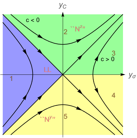
Figure 1: (Color online) Solution of Kosterlitz-Thouless equations (11). Different symbols and colors depict Ising phases N^z (green region) and N^y (yellow region) and the critical Luttinger liquid phase (purple region) according to the RG flow criteria summarized in Table 1.

Region	1	2	3	4	5
$y_{C}(0)$	$+/-$	$\;\;+\;\;$	$\;\;+\;\;$	$\;\;-\;\;$	$\quad-\quad$
$y_{\sigma}(0)$	$-$	$-$/$+$	$+$	$+$	$-$/$+$
$C$	$+$	$-$	$+$	$+$	$-$
$y_{C}(\ell^{*})$	0	$\;+\infty\;$	$\;+\infty\;$	$\;-\infty\;$	$\;-\infty\;$
$y_{\sigma}(\ell^{*})$	finite	$\;+\infty\;$	$\;+\infty\;$	$\;+\infty\;$	$\;+\infty\;$
$y_{B}(\ell^{*})$	finite	finite	finite	finite	finite
State	LL	“$N^{z}$”	“$N^{z}$”	“$N^{y}$”	“$N^{y}$”

Table 1: Signs and values of $y_{C}$, $y_{\sigma},andC$ corresponding the KT flow in Fig. 1. Here $\ell^{*}$ is the critical RG scale at which one (or several) coupling constant reaches the strong-coupling limit (and becomes of order one).

II.2 Two-stage RG

Renormalization group equations for coupling constants of the backscattering interaction (3) are obtained with the help of the operator product expansion Fradkin (2013); Starykh et al. (2005) technique and read

$$\begin{split}\frac{dy_{x}}{dl}&=y_{y}y_{z},\quad\frac{dy_{y}}{dl}=y_{x}y_{z}+y_{A}^{2},\\ \frac{dy_{z}}{dl}&=y_{x}y_{y},\quad\frac{dy_{A}}{dl}=y_{y}y_{A}.\\ \end{split}$$ (8)

The presence of oscillating $e^{it_{\varphi}x}$ factors implies the appearance of the spatial scale, proportional to $1/t_{\varphi}$, and, correspondingly, of the RG scale $\ell_{\varphi}$

$$\begin{gathered}\ell_{\varphi}=\ln(\frac{1}{a_{0}t_{\varphi}})=\ln[\frac{1}{20.4}\frac{\pi}{2}\frac{1}{\sqrt{D^{2}+h^{2}}}].\end{gathered}$$ (9)

where, $a_{0}=20.4a$ is the ultraviolet RG cutoff length scale Garate and Affleck (2010) (see Ref. Garate and Affleck, 2010 for details of how the choice of the initial value for $g_{\rm bs}$ also determines $a_{0}$).

For $\ell<\ell_{\varphi}$ oscillations due to $e^{it_{\varphi}x}$ can be neglected and the full set of RG equations (8) has to be solved numerically. Once RG time $\ell>\ell_{\varphi}$, strong oscillations in $H_{A}$ and $H_{B}$ result in the disappearance of these terms from the Hamiltonian. Correspondingly, we can set $y_{A}(\ell)=0$ and $y_{B}(\ell)=0$ in the RG equations. Therefore, at this second stage, the RG equations simplify to [see Eq. (4)]

$$\frac{dy_{C}}{d\ell}=y_{C}y_{\sigma},\;\;\;\frac{dy_{\sigma}}{d\ell}=y_{C}^{2}.\\$$ (10)

These are the well-known Kosterlitz-Thouless (KT) equations, the analytic solution of which is summarized in Appendix C. The initial values of backscattering couplings at the second stage are

$$\begin{split}y_{C}(\ell_{\varphi})&=(y_{x}(\ell_{\varphi})-y_{y}(\ell_{\varphi}))/2\\ &\to-\frac{g_{\rm bs}}{4\pi v}[(1+\frac{\lambda}{2})\cos\theta^{-}-1+\frac{\lambda}{2}],\\ y_{\sigma}(\ell_{\varphi})&=-y_{z}(\ell_{\varphi})\to\frac{g_{\rm bs}}{2\pi v}[(1+\frac{\lambda}{2})\cos\theta^{-}-\frac{\lambda}{2}],\\ C&=y_{\sigma}(\ell_{\varphi})^{2}-y_{C}(\ell_{\varphi})^{2},\\ \end{split}$$ (11)

where $\cos\theta^{-}=(h^{2}-D^{2})/(h^{2}+D^{2})$ and $C$ is the constant of motion, with $dC/d\ell=0$. Expressions following the right-arrow sign $\rightarrow$ in the above equations pertain to the situation when the first stage of RG flow, $\ell<\ell_{\varphi}$, can be skipped. This is the case of strongly oscillating $e^{it_{\varphi}x}$ factors in Eq. (3), when all the oscillating terms in the backscattering Hamiltonian can be omitted from the outset and, correspondingly, $y_{a}(\ell_{\varphi})\approx y_{a}(0)$. Formally, this limit corresponds to a negative $\ell_{\varphi}$ as defined in Eq. (9).

II.3 Ising orders

We have identified five distinct regions with different signs of $y_{C,\sigma}$ and integration constant $C$, which result in different RG flows. The boundaries of these regions depend on the initial values of $y$’s and $C$. When the first-stage flow can be skipped, which happens for sufficiently large $h_{\rm eff}$ such that formally $\ell_{\varphi}<0$, as discussed at the end of Sec. II.2, then the dependence on initial values can be directly translated into that on $h/D$ ($\cos\theta^{-}$) and $\lambda$ ($\Delta$ and $D/J$). These results are summarized in Table 1 and Fig. 1, which shows what orders are promoted in different regions.

Small $t_{\varphi}$ results in $\ell_{\varphi}>0$ and a two-step RG analysis is required, as explained above. Once the RG equations (8) are integrated to $\ell=\ell_{\varphi}$, all the oscillating terms must be dropped and only two momentum-conserving terms, $H_{c}$ and $H_{\sigma}$, remain present in the Hamiltonian.

In terms of Abelian fields $(\varphi,\vartheta)$, the interaction $H_{C}$ is nonlinear, $H_{C}\propto y_{C}\cos[2\sqrt{2\pi}\vartheta]=y_{C}\cos[2\beta\vartheta]$, while $H_{\sigma}\propto(\partial_{x}\varphi)^{2}-(\partial_{x}\vartheta)^{2}$ and describes renormalization of $\beta$ (see Appendix E.1). (We neglect marginal renormalization of the spinon’s velocity $v\to v\sqrt{1-y_{\sigma}^{2}/2}$.) The ground state of the chain is determined by the ordering of the $\vartheta$ field.

It is important to understand how the chiral rotation, which led to (3), affects staggered magnetization and dimerization. Arguments in Appendix B show that staggered magnetization ${\bf N}$ and dimerization $\epsilon$ in the laboratory frame are related to those in the rotated frame, ${\bm{\mathcal{N}}}$ and $\xi$, as follows:

$${\bm{N}} = (-{\cal N}^{z},\cos\theta_{0}{\cal N}^{y}+\sin\theta_{0}\xi,{\cal N}^{x}),$$

$$\epsilon = \cos\theta_{0}\xi-\sin\theta_{0}{\cal N}^{y}.$$ (12)

Further, a shift of the $\varphi$ field by $t_{\varphi}x$ [Eq. (31)] introduces a $t_{\varphi}x$ dependence in the arguments of fields ${\cal N}^{z}$ and $\xi$ [Eq. (33)], but does not affect the ${\cal N}^{x,y}$ pair.

Flow of the KT equations (10) to strong coupling implies development of the expectation value for the $\vartheta$ field. When $y_{C}\to+\infty$ for $\ell\to\infty$, the energy is minimized by $\sqrt{2\pi}\vartheta=(2k_{1}+1)\pi/2$, with $k_{1}$ an integer, and ${\cal N}^{x}\propto-\sin\sqrt{2\pi}\vartheta\neq 0$. This means that in the original frame there is an Ising order $N^{z}\neq 0$, and following Ref. Garate and Affleck, 2010 we name this state “$N^{z}$”. The long-range order (staggered magnetization) in the laboratory frame is commensurate,

$$\langle\bm{N}(x)\rangle\propto\langle\sin(\sqrt{2\pi}\vartheta)\rangle{\bf z}\propto(-1)^{k_{1}+1}{\bf z}.$$ (13)

In the case of $y_{C}\to-\infty$ the energy is minimized by $\sqrt{2\pi}\vartheta=k_{2}\pi$, with $k_{2}$ an integer, and ${\cal N}^{y}\propto\cos\sqrt{2\pi}\vartheta\neq 0$. Therefore, the Ising order is now along the ${\bf y}$ axis, $N^{y}\neq 0$, and we name it $N^{y}$. In addition, according to Eq. (12), the finite expectation value of ${\cal N}^{y}$ implies finite staggered magnetization $\epsilon$. Garate and Affleck (2010) Therefore, the $N^{y}$ phase is characterized by the coexistence of commensurate Ising Néel and dimerization orders

$$\begin{split}\langle\bm{N}(x)\rangle&\propto\cos\theta_{0}\langle\cos(\sqrt{2\pi}\vartheta)\rangle{\bf y}\propto\cos\theta_{0}(-1)^{k_{2}}{\bf y},\\ \epsilon&\propto-\sin\theta_{0}\langle\cos(\sqrt{2\pi}\vartheta)\rangle\propto\sin\theta_{0}(-1)^{k_{2}+1}.\end{split}$$ (14)

Finally, a gapless regime of $y_{C}\to 0$ for $\ell\to\infty$ is also possible Garate and Affleck (2010). Here the Hamiltonian is purely quadratic and describes a critical LL phase with algebraic correlations even though the spin rotational symmetry is fully broken Garate and Affleck (2010); Giamarchi and Schulz (1988); (see Appendix E.3 for detailed arguments). As described in the Introduction, the LL state is the quantum version of the classical chiral soliton lattice phase. This is a critical state with incommensurate (and anisotropic) spin correlations which decay algebraically with distance.

III Phase diagram of the quantum model

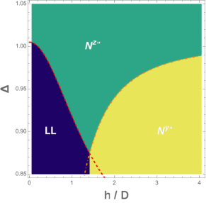
Figure 2: (Color online) Phase diagram for the case of relatively strong DM interaction $D/J=0.1$. Larger $D$ promotes $N^{z}$ state. The two phase boundaries are given by Eq. (15) (orange dot-dashed line), and Eq. (16) (red dashed line). The phase boundary between LL and $N^{y}$ is located at $h/D=\sqrt{2}$ and is independent of $\Delta$.

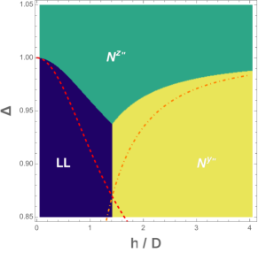
Figure 3: (Color online) Phase diagram for the case of a small DM interaction $D/J=0.01$ obtained via a two-stage RG process. At the first stage RG equations (8) are integrated numerically. Second-stage equations (10) are then solved analytically. The phase boundaries given by Eq. (15) (orange dot-dashed line) and Eq. (16) (red dashed line) are seen to deviate significantly from the actual ones. This shows the importance of the first-stage flow in the case of small and intermediate $D/J$.

The $\Delta-(h/D)$ phase diagrams are obtained by solving the RG equations and are presented in Figs. 2 and 3. Figure 2 is obtained under the condition that the first-stage RG flow can be skipped, due to the fact that $\ell_{\varphi}<0$ in Eq. (9), which happens for sufficiently large $D$ and/or $h$. Here we choose $D/J=0.1$. In this situation we can determine the ground state simply by studying the initial conditions of the KT equations according to the chart in Table 1 and Fig. 1.

When $\ell_{\varphi}>0$ oscillations develop over some finite lengthscale and one needs to integrate the first-stage RG equations (8) numerically for the interval $0\leq\ell\leq\ell_{\varphi}$. At the end of the first stage we obtain $y_{C}(\ell_{\varphi})$, $y_{\sigma}(\ell_{\varphi})$, and $C=y_{\sigma}^{2}(\ell_{\varphi})-y_{C}^{2}(\ell_{\varphi})$, which serve as initial values of the couplings for the second-stage, KT part, of the RG flow. This is the case of the $D/J=0.01$ phase diagram for which is presented in Fig. 3.

By comparing the phase diagrams in Figs. 2 and 3, we observe that large $D$ promotes the $N^{z}$ state, which is consistent with the numerical DMRG result in Fig. 4.

Next we study phase boundaries between different phases. Figure 1 shows that the phase transition between $N^{y}$ and $N^{z}$ states is related to the initial values of $y_{C}$ and $y_{\sigma}$. The coupling $y_{C}(0)$ has opposite signs in the regions $3$ and $4$. Therefore in the $\Delta-h/D$ phase diagram this boundary corresponds a critical value $\Delta_{c1}$ at which $y_{C}(0)=0$ and $C=y_{\sigma}^{2}(0)>0$. These conditions indicate that the boundary is described by $D/h=\sqrt{\lambda/2}$, which leads to the explicit expression for it:

$$\Delta_{c1}=1+\frac{1}{2}(\frac{D}{J})^{2}-\frac{2}{c}(\frac{D}{h})^{2}.$$ (15)

For a fixed $D$, a larger field $h$ leads to a greater $\Delta_{c1}$, which is illustrated as an orange dot-dashed line in Figs. 2 and 3. Figure 2 shows excellent agreement of the obtained phase transition line with the numerical solution of RG equations, due to the fact that in this case the first stage of RG flow is not required. Interestingly, the limit of $D\to 0$, corresponding to $h/D\to\infty$ in the above figures, is described by our theory as well, as we explain in Appendix D. In that case one deals with the $XXZ$ model in the transverse magnetic field for which the critical line separating the two Ising phases $N^{y}$ and $N^{z}$ is reduced to the horizontal asymptote $\Delta_{c1}=1$, in agreement with the previous study in Ref. Dmitriev et al., 2002.

The boundary between the gapless LL and Ising $N^{z}$, according to Table 1, happens at $C=0$, $y_{C}(0)>0$, and $y_{\sigma}(0)<0$. Therefore, we have the relation that $y_{\sigma}(0)=-y_{C}(0)$. This gives the critical $\Delta_{c2}$

$$\Delta_{c2}=1+\frac{1}{2}(\frac{D}{J})^{2}-\frac{2}{c}\frac{1}{1+2(D/h)^{2}}.$$ (16)

Therefore, in contrast to Eq. (15), a larger field $h$ results in a smaller $\Delta_{c2}$. This result is also confirmed in Figs. 2 and 3.

Finally, the transition between the LL and Ising $N^{y}$ is described by $C=0$, $y_{C}(0)<0$, and $y_{\sigma}(0)<0$. This gives $y_{C}(0)=y_{\sigma}(0)$, which is satisfied by $\cos\theta^{-}=1/3$ and $\lambda\geq 1$. This condition implies that transition between the LL and $N^{y}$ is a vertical line located at $(h/D)_{c3}=\sqrt{2}$, which is again confirmed by numerical solution of the RG equations in Figs. 2 and 3. Different from the other two boundaries, the one between the LL and $N^{y}$ is independent of $\Delta$, and this is consistent with the classical analysis in Ref. Garate and Affleck, 2010. The constraint $\lambda\geq 1$ implies that this boundary exists only for $\Delta\leq\Delta_{t}\equiv 1+(D/J)^{2}/2-1/c$. The crossing point of the critical lines $\Delta_{c1}$ and $\Delta_{c2}$ also gives the condition $(h/D)_{c3}=\sqrt{2}$. The triple point where three phases intersect is at $h/D=\sqrt{2}$ and $\Delta_{t}$. For $D/J=0.1$ in Fig. 2 it is evaluated to be at $\Delta_{t}\simeq 0.874$.

The main message of this section is that a strong DM interaction, acting jointly with the transverse magnetic field, causes significant modification of the classical phase diagram and works to stabilize Ising $N^{z}$ order well beyond its classical domain of stability (given by $\Delta>1$), in agreement with the field-theoretic predictions of Refs. Gangadharaiah et al., 2008 and Garate and Affleck, 2010.

IV Numerical studies

In this section, we will determine the ground-state properties of the model system in Eq. (1) by an extensive and accurate DMRGWhite (1992, 1993); Schollwöck (2005) simulation. Here we consider a system with a total number of sites $L$ up to $L=1600$ and perform ten sweeps by keeping up to $m=400$ DMRG states with a typical truncation error of order $10^{-9}$. In addition, we have also carried out an independent infinite time-evolving block decimation (iTEBD) Vidal (2003, 2004, 2007) simulations with the same bond dimension and the same lengths as for the correlation function calculations. Our iTEBD results agree fully with our DMRG results (see Fig.4 below).

Our principal results are summarized in the phase diagram in Fig.4 at $D/J=0.05$ and $D/J=0.1$. Changing the parameters $\Delta$ and $h/D$, we find three distinct phases, including a gapless LL phase and two ordered phases: the Néel Ising ordered $N^{z}$ (Ising order along the $z$ axis) and $N^{y}$ (Ising order along the $y$ axis) phases. Our numerical results show that the DM interaction stabilizes the $N^{z}$ Ising order which extends into the $\Delta<1$ region, while the $N^{y}$ Ising order gets suppressed by the DM interaction and gives way to the LL phase for a relatively small transverse magnetic field $h\lesssim D$. These results agree well with the field-theoretic predictions described in Secs. II and III, although with slightly different phase boundaries due to significant finite-size effects, which are described in more detail in Sec. V.

To characterize distinct phases of the phase diagram, we measure magnetic correlations in the ground state by evaluating the equal time spin structure factor $M_{s}^{\alpha}(k)=\frac{1}{L}\sum^{L}_{ij}e^{\imath k(r_{i}-r_{j})}\langle S^{\alpha}_{i}S^{\alpha}_{j}\rangle$, where $\alpha=x,y,z$ denotes different spin components. The structure factor is peaked at $k=\pi$ in both the $N^{z}$ and $N^{y}$ phases, corresponding to the commensurate Néel Ising order along the $z$ axis and $y$ axis, respectively. To quantitatively analyze this order, we perform an extrapolation of the spin order parameter $N^{\alpha}(k)=\sqrt{M^{\alpha}_{s}(k)/L}$ to the thermodynamic limit ($L=\infty$) according to the generally accepted form

$$N^{\alpha}(k,L)=N^{\alpha}(k,\infty)+\frac{a}{\sqrt{L_{1/2}}}+\frac{b}{L_{1/2}}$$ (17)

where $a$ and $b$ are fitting parameters (see Appendix F for details). The structure factor for a finite system of length $L$ is calculated by using only the central $L_{1/2}=L/2$ part of finite systems. In addition to the spin order, we also calculate the dimer structure factor $M_{d}(k)=\frac{1}{L}\sum^{L}_{ij}e^{\imath k(r_{i}-r_{j})}\langle B_{i}B_{j}\rangle$, where $B_{i}=\textbf{S}_{i}\cdot\textbf{S}_{i+1}$ denotes the bond operator (see Fig. 5 for an example of the $M_{d}(k)$ data). Staggered dimerization $\epsilon(x)$, introduced in (29), represents the low-energy limit of the staggered part of the bond operator, $B_{i}\to{\cal B}(x)+(-1)^{x}\epsilon(x)$, while its uniform part ${\cal B}$ represents an average bond energy.

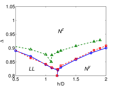
Figure 4: (Color online) Ground-state phase diagram of the system in Eq.(1) at $D/J=0.1$ as determined by DMRG (open circles) and iTEBD (open squares) calculations for system with $L$=1200 sites. For comparison, the phase diagram at $D/J=0.05$ is also provided obtained by DMRG simulation for the system with $L=800$ sites (open triangles). The lines are guides for the eye.

To charaterize distinct phases in the phase diagram, we first show examples of both spin and dimer structure factors of the systems with length $L=1600$ in Fig. 5.

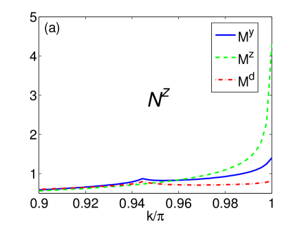
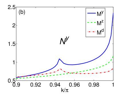
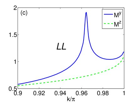
Figure 5: (Color online) Structure factors $M_{s}^{y}$ (blue solid line) and $M_{s}^{z}$ (green dashed line) with $L=1600$ and $M_{d}$ (red dot-dashed line) with $L=1200$ (a) in the $N^{z}$ phase at $\Delta=1.1$, $D/J=0.1$, and $h/J=0.2$, (b) in the $N^{y}$ phase at $\Delta=0.7$, $D/J=0.1$, and $h/J=0.2$, and (c) in the $LL$ phase at $\Delta=0.7$, $D/J=0.1$, and $h/J=0.075$.

IV.1 The $N^{z}$ phase

The $N^{z}$ phase is well understood for the case $\Delta>1$ without a DM interaction. A finite DM interaction pushes the phase boundary to a lower $\Delta$ value due the renormalization of the effective anisotropy, which can be seen in the phase diagram. Figure 5(a) plots the structure factors at $\Delta=1.1$, $D/J=0.1$, and $h/J=0.2$, where the structure factor $M^{z}_{s}(k)$ shows a clear peak at commensurate momentum $k=\pi$, indicating the presence of the Nèel Ising order. In contrast, the structure factor $M^{y}_{s}(k)$ has two smaller peaks, one at commensurate momentum $k=\pi$ and another at incommensurate momentum $k=k^{\star}<\pi$. However, since both peaks in the $M^{y}_{s}(k)$ structure factor are substantially smaller than the peak in $M^{z}_{s}(k)$ at commensurate $k=\pi$, we conclude that at this point the spin chain is the $N^{z}$ phase, with no $N^{y}$ kind of Ising order.

IV.2 The $N^{y}$ phase

When $\Delta$ is small while $h$ is sufficient large, the system enters into the $N^{y}$ phase. This phase is characterized by a dominant peak of the structure factor $M^{y}_{s}(k)$ at commensurate momentum $k=\pi$, while peaks in $M^{z}_{s}(k=\pi)$ and $M^{y}_{s}(k=k^{\star})$ are much smaller [see Fig. 5(b)]. Note that the $N^{y}$ Néel Ising order, which is also present in the system without a DM interaction, is suppressed by the finite DM interaction, especially for $h\leq D$. See Appendix D for an analytical explanation of this.

IV.3 The LL phase

The system is in the LL phase when both $\Delta$ and $h$ are small enough, and is characterized by the dominant peak in the structure factor $M^{y}_{s}(k)$ at the incommensurate momentum $k=k^{\star}<\pi$ as shown in Fig. 5(c). For example, the peak is at $k^{*}\approx 0.965\pi$ for $\Delta=0.7$, $D/J=0.1$, and $h/J=0.075$. For the same set of parameters, the field theory predicts the peak to be at $k=\pi\pm t_{\varphi}$, with $t_{\varphi}=\sqrt{h^{2}+D^{2}}/(\pi J/2)$ [see (33) and (E.3)]. This prediction translates into $k^{*}=0.975\pi$, which is consistent with the numerical result. Notice that our numerical calculations give a slightly smaller $k^{*}$, which is caused by the difference in spinon velocity $v$ from the zero field value $\pi J/2$ and finite-size effects. Similar to $M^{y}_{s}(k)$, the dimer structure factor also exhibits a two-peak feature at both commensurate $k=\pi$ and incommensurate momenta $k=k^{\star}<\pi$. This is a direct consequence of the chiral rotation (23) which mixes up staggered magnetization and dimerization operators as Eqs. (29) and (27) [equivalently, (12)] show.

Having characterized the distinct phases, now we can try to determine the phase boundary between them.

IV.4 The $N^{y}$-$N^{z}$ boundary

The phase boundary between the two Ising phases is determined by the order parameters $N^{y}(\pi)$ and $N^{z}(\pi)$, which should saturate to a finite nonzero value in the thermodynamic limit in the $N^{y}$ and $N^{z}$ phases, correspondingly, and vanish elsewhere. Unfortunately, due to large finite-size effects (see Sec. V for details), the order parameters tend to behave continuously across the anticipated phase boundary, even though their values in the “wrong” phase become very small. We therefore try to identify the phase boundary by looking for the crossing point where the two order parameters take the same value since the $N^{z}$ Ising order dominates at larger $\Delta$ while the $N^{y}$ order wins at smaller $\Delta$. An example of determining the phase boundary in this way is shown in Fig. S1(a) in the Appendix F.

IV.5 LL-Ising boundary

In the LL phase all order parameters vanish in the thermodynamic limit. Unfortunately, again due to strong finite-size effects, an unambiguous identification of this phase is difficult since both Ising order parameters remain nonzero, although really small, inside it. We observe that in both $N^{y}$ and LL phases, the spin structure factor $M_{s}^{y}(k)$ develops peaks at commensurate momentum $k=\pi$ and at incommensurate momentum $k=k^{\star}<\pi$ (see Fig. 5). This is a direct consequence of Eqs.(12) and (27), which show that $N^{y}\sim\cos\theta_{0}{\cal N}^{y}+\sin\theta_{0}\xi$. While ${\cal N}^{y}$ is peaked at zero momentum [which means that its contribution to spin density $S^{y}\sim(-1)^{x}N^{y}$ is peaked at momentum $\pi$], the rotated dimerization operator $\xi$ is peaked at $\pm t_{\varphi}$ [see Eqs.(31) and (33)]. Therefore, $M_{s}^{y}(k)$ is expected to have peaks at both $k=\pi$ and $k^{*}=\pi-t_{\varphi}$. A similar two-peak structure, with maxima at momenta $\pi$ (coming from ${\cal N}^{y}$) and $k^{*}$ (coming from $\xi$), shows up in the dimer structure factor $M_{d}(k)$, in full agreement with the second line of (12). Figures 5 (a) and (b) show the corresponding numerical data.

Inside the $N^{y}$ phase the dominant peak of $M_{s}^{y}$ is at $k=\pi$, suggesting the well developed Néel order of the $N^{y}$ kind. In contrast, deep inside the LL phase, $M_{s}^{y}(k^{*})$, which comes from power-law correlations of the rotated dimerization operator $\xi$, dominates over the peak at $\pi$. This numerical finding is fully consistent with our low-energy bosonization calculation in Eq. (E.3), which shows that spin correlations caused by rotated operators $\xi$ and ${\cal N}^{z}$ are the slowest-decaying ones. Therefore, the phase boundary between the LL and $N^{y}$ phases can be identified from the condition $M^{y}_{s}(k=k^{\star})=M^{y}_{s}(k=\pi)$. The resulting phase boundary agrees well with the theoretical prediction. Similarly, the boundary between the LL and $N^{z}$ phases is determined by $M^{y}_{s}(k=k^{\star})=M^{z}_{s}(k=\pi)$, [see Fig. S1b]. Since $M^{y}_{s}$ shows a dominant peak at $k=k^{\star}$ in the LL phase while the ${\cal N}^{z}$ phase has a dominant order at $k=\pi$, the phase boundary between these two phases can be determined by the crossing point of the above quantities.

Further quantitative agreement can be established by comparing numerical data for $k^{\star}$, extracted from $M_{s}^{y}(k)$ and $M_{d}(k)$ data, with the analytical prediction $k^{*}=\pi-t_{\varphi}=\pi-\sqrt{D^{2}+h^{2}}/v$, as shown in Fig. 6. The small difference between the measured and the predicted $k^{*}$ values is probably due to our omission of the velocity renormalization by marginal operators.

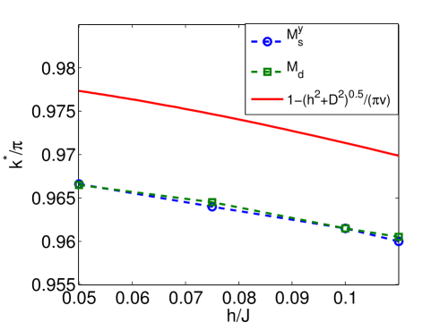
Figure 6: (Color online) Dependence of the incommensurate peak momentum $k^{\star}$ in the spin structure factor $M^{y}_{s}(k)$ (blue circles) and dimer structure factor $M_{d}(k)$ (green squares) as a function of the transverse magnetic field $h$ at $D/J=0.1$. The red line denotes the theoretical prediction, we used $v=\pi J/2$.

Finally, we have also calculated the phase diagram of the system with a smaller DM interaction $D/J=0.05$. The phase diagram for the $L=800$ chain is shown in Fig. 4 by a green dashed line. Compared with the larger DM interaction $D/J=0.1$ case, the phase boundaries for both the $N^{z}$-$LL$ and $N^{z}$-$N^{y}$ phase transitions move to higher $\Delta$ values, in qualitative agreement with theoretical expectations (see phase diagrams in Figs. 2 and 3 for a similar comparison).

V Analytical understanding of finite size effects in DMRG study

Our formulation provides a convenient way to understand some of the finite-size effects unavoidable in the numerical study of the problem. Here we focus on the case of a relatively strong DM interaction $D/J=0.1$, analytical and numerical phase diagrams for which are presented in Figs. 2 and 4, correspondingly.

By solving the RG equations (10) we obtain the critical RG scale $\ell^{*}$ at which the order develops fully, namely, $|y_{C}(\ell^{*})|=1$. We find that $\ell^{*}$ grows rapidly as $\Delta$ approaches the phase boundary between the $N^{y}$ and $N^{z}$ states, as shown in Fig. 7, with $\ell\approx 50$ near the critical point. However the finite size of the system used in the DMRG study, $L=1600$ in units of the lattice spacing $a$, corresponds to a much smaller RG scale of $\ell_{s}=\ln[1600]=7.37$. Therefore the RG scales greater than $\ell_{s}$ are not accessible for the DMRG. In other words, if we associate the correlation length $\xi=ae^{\ell^{*}}$ with the order which develops at $\ell^{*}$, and if it happens that $\ell^{*}>\ell_{s}=7.37$, then the DMRG simulations will not be sensitive to the development of the long-range order in this case. This is the basic explanation of the unavoidable difficulty one encounters in numerical determination of the phase boundaries between various phases.

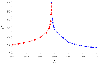
Figure 7: (Color online) Critical RG $\ell^{*}$ for which $|y_{c}(\ell^{*})|=1$ (obtained by solving the KT equations; see Appendix C) as a function of the $XXZ$ anisotropy $\Delta$. Here $D/J=0.1$ and $h/J=0.2$. The system is in the $N^{y}$ phase (red line) for $\Delta<\Delta_{c}\simeq 0.94$ [the phase boundary $\Delta_{c}$ is determined from Eq. (15)], while at $\Delta>\Delta_{c}$ the system enters the $N^{z}$ phase (blue line). Near the transition point, $\ell^{*}\gg\ell_{s}=7.37$.

In addition to calculating the $\ell^{*}$ associated with the development of long-range order, we can also calculate the order parameters for the $N^{y}$ and $N^{z}$ phases developing in the system as functions of the running RG scale $\ell$. Appendix E describes how it is done. We show there that the required order parameters are given by

$$\begin{gathered}\langle N^{y}\rangle=\langle\text{Re}[e^{i\beta\vartheta/2}]\rangle,\quad\langle N^{z}\rangle=\langle\text{Im}[e^{i\beta\vartheta/2}]\rangle.\end{gathered}$$ (18)

Equation (58) shows the explicit form of the order parameters in terms of running couplings $y_{C,\sigma}(\ell)$. Figure 8 illustrates our results. It shows the order parameters $\langle N^{y,z}\rangle$ which are evaluated at the maximum possible for our chain RG scale $\ell=\ell_{s}$. Observe that, in agreement with the numerical data in Fig. S1(a), there is a noticeable asymmetry between these two order parameters: The order parameter of the $N^{y}$ phase is smaller than that of the $N^{z}$ phase.

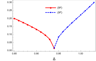
Figure 8: (Color online) Order parameters as a function of $\Delta$ for two ordered states $N^{y}$ and $N^{z}$, at $D/J=0.1$, $h/J=0.2$, and RG length scale $\ell=\ell_{s}$. Here $\Delta$ is near the phase boundary $\Delta_{c}\simeq 0.94$ (determined from Eq. (15)). See the main text and Appendix E for details.

VI Conclusions

Our extensive DMRG study shows an excellent agreement with the analytical investigation based on the RG analysis of the weakly perturbed Heisenberg chain. We have worked out a full phase diagram of the model in the $\Delta-(h/D)$ plane. Our numerical findings match predictions of Ref. Garate and Affleck, 2010 well and confirm the prevalence of $N^{z}$ Néel Ising order in the regime of comparable DM and magnetic field magnitudes Gangadharaiah et al. (2008). In addition, we find that significant finite-size corrections observed numerically are well explained by the logarithmic slowness of the KT RG flow. As a result of that, very large RG scales $\ell^{*}$, far exceeding those set by the finite length $L$ of the chain used in the DMRG, are required to reach the Ising-ordered phases.

Our numerical data also confirm the existence of the critical Luttinger liquid phase with fully broken spin-rotational invariance. This phase with dominant incommensurate spin and dimerization power-law correlations is a quantum analog of the classical chiral soliton lattice.

Our findings open up the possibility of an experimental check of theoretical predictions in quasi-one-dimensional antiferromagnets with a uniform DM interaction Hälg et al. (2014); Smirnov et al. (2015). The idea is to probe the spin correlations at a finite temperature above the critical ordering temperature of the material when interchain spin correlations, which drive the three-dimensional ordering, are not important while individual chains still possess anisotropy of spin correlations, sufficient for experimental detection, caused by the uniform DM interaction. Under these conditions one should be able to probe the fascinating competition between the uniform DM interaction and the transverse external magnetic field.

Appendix A Bosonization

The low-energy description is provided by the parametrizationGangadharaiah et al. (2008) ${\bm{S}}(x)\approx{\bm{J}}(x)+(-1)^{n}{\bm{N}}(x)$, where ${\bm{J}}={\bm{J}}_{L}+{\bm{J}}_{R}$, with ${\bm{J}}_{L}(x)$ and ${\bm{J}}_{R}(x)$ are the uniform left- and right-moving spin currents, and ${\bm{N}}(x)$ is the staggered magnetization (our order parameter). Here $x=na$ in terms of lattice constant $a$. These fields are expressed in terms of bosonic fields $(\phi,\theta)$ [this expansion is not specific to the SU(2), Heisenberg, point and can be generalized easily to a more general $XXZ$ Hamiltonian],

$$\begin{gathered}J_{R}^{+}=\frac{1}{2\pi a}e^{-i\sqrt{2\pi}(\phi-\theta)},\;J_{L}^{+}=\frac{1}{2\pi a}e^{i\sqrt{2\pi}(\phi+\theta)},\\ J_{R}^{z}=\frac{\partial_{x}\phi-\partial_{x}\theta}{2\sqrt{2\pi}},\;J_{L}^{z}=\frac{\partial_{x}\phi+\partial_{x}\theta}{2\sqrt{2\pi}},\end{gathered}$$ (19)

and

$${\bm{N}}=A(-\sin[\sqrt{2\pi}\theta],\;\cos[\sqrt{2\pi}\theta],\;-\sin[\sqrt{2\pi}\phi]).$$ (20)

Here, $A\equiv\gamma/\pi a_{0}$ and $\gamma=\langle\cos(\sqrt{2\pi}\phi_{\rho})\rangle\sim O(1)$ is determined by gapped charged modes of the chain. The Hamiltonian in Eq. (1) is approximated in the low energy limit as Gangadharaiah et al. (2008); Schnyder et al. (2008); Garate and Affleck (2010)

$$H=H_{0}+V+H_{\rm bs},$$ (21)

where

$$\begin{split}H_{0}&=\frac{2\pi v}{3}\int\mathrm{d}x({\bm{J}_{R}}\cdot{\bm{J}_{R}}+{\bm{J}_{L}}\cdot{\bm{J}_{L}}),\\ V&=-{D}\int\mathrm{d}x(J_{R}^{z}-J_{L}^{z})-h\int\mathrm{d}x(J_{R}^{x}+J_{L}^{x}),\\ H_{\rm bs}&=-g_{\rm bs}\int\mathrm{d}x[J_{R}^{x}J_{L}^{x}+J_{R}^{y}J_{L}^{y}+(1+\lambda)J_{R}^{z}J_{L}^{z}],\\ \end{split}$$ (22)

where $\lambda$ is the total $XXZ$ anisotropy described by Eq. (7).

Appendix B Chiral rotation

The system Hamiltonian is described in Eq. (22). It is convenient to exploit the extended symmetry of $H_{0}$ and treat both vector perturbations $h$ and $D$ equally by performing a chiral rotation of spin currents about the ${y}$ axis Gangadharaiah et al. (2008); Schnyder et al. (2008); Garate and Affleck (2010)

$${\bm{J}}_{R/L}={\cal R}(\theta_{R/L}){\bm{M}}_{R/L},$$ (23)

with ${\bm{M}}_{R/L}$ is the spin current in the rotated frame, and $\cal R$ is the rotation matrix,

$$\begin{gathered}{\cal R}(\theta_{R/L})=\begin{pmatrix}\cos\theta_{R/L}&0&\sin\theta_{R/L}\\ 0&1&0\\ -\sin\theta_{R/L}&0&\cos\theta_{R/L}.\end{pmatrix},\end{gathered}$$ (24)

where

$$\begin{gathered}\theta_{R}=\theta_{0}+\pi/2,\;\theta_{L}=-\theta_{0}+\pi/2,\;\theta_{0}\equiv\arctan\left(\frac{-D}{h}\right).\end{gathered}$$ (25)

Via this chiral rotation, vector perturbation $V$ in Eq. (22) becomes

$$\begin{split}V&=-\sqrt{D^{2}+h^{2}}\int\mathrm{d}x(M_{R}^{z}+M_{L}^{z})\\ &=-\frac{\sqrt{D^{2}+h^{2}}}{\sqrt{2\pi}}\int\mathrm{d}x\partial_{x}\varphi.\end{split}$$ (26)

The staggered magnetization transforms as

$${\bm{N}}=(-{\cal N}^{z},\cos\theta_{0}{\cal N}^{y}+\sin\theta_{0}\xi,{\cal N}^{x}),$$ (27)

Here ${\bm{\mathcal{N}}}$ and $\xi$ denote the staggered magnetization and dimerization in the rotated frame. They, as well as rotated spin currents ${\bm{M}}_{R/L}$, are expressed in terms of Abelian bosonic fields $\varphi$ and $\vartheta$. Staggered magnetization ${\bf N}$ in (20), staggered dimerization $\epsilon=({\gamma}/{\pi a_{0}})\cos[\sqrt{2\pi}\phi]$, and spin currents ${\bm{J}}_{R/L}$ are written in terms of a $(\phi,\theta)$ pair, as Eqs. (19) and (20) show. Therefore, in the rotated frame

$${\bm{\mathcal{N}}}=\frac{\gamma}{\pi a_{0}}(-\sin\sqrt{2\pi}\vartheta,\cos\sqrt{2\pi}\vartheta,-\sin\sqrt{2\pi}\varphi)$$ (28)

and $\xi=({\gamma}/{\pi a_{0}})\cos\sqrt{2\pi}\varphi$.

The relation (27) is obtained by observing that chiral rotation (23) of vector currents corresponds to the following rotation of Dirac spinors Garate and Affleck (2010); Starykh (2010) $\Psi_{R/L,s}=e^{-i\theta_{R/L}\sigma^{y}/2}\tilde{\Psi}_{R/L,s}$ in terms of which spin currents are expressed Starykh et al. (2005) as $J^{a}_{R/L}=\Psi_{R/L}^{+}\sigma^{a}\Psi_{R/L}/2$ and $M^{a}_{R/L}=\tilde{\Psi}_{R/L}^{+}\sigma^{a}\tilde{\Psi}_{R/L}/2$. The (original) staggered magnetization, $N^{a}=(\Psi_{R}^{+}\sigma^{a}\Psi_{L}+\Psi_{L}^{+}\sigma^{a}\Psi_{R})/2$, rotates into (27). Similarly, staggered dimerization $\epsilon(x)\sim(-1)^{x/a}{\bf S}(x)\cdot{\bf S}(x+a)$ transforms as

$$\epsilon=\cos\theta_{0}\xi-\sin\theta_{0}{\cal N}^{y}.$$ (29)

The rotation (23) transforms the backscattering Hamiltonian in (22) into,

$$\begin{split}{H}_{\rm bs}=&2\pi v\int\mathrm{d}x\Big{[}\sum_{\alpha}y_{\alpha}M_{R}^{\alpha}M_{L}^{\alpha}+\\ &+y_{A}(M_{R}^{z}M_{L}^{x}-M_{R}^{x}M_{L}^{z})\Big{]},\end{split}$$ (30)

where $\alpha=x,y,z$ and the initial values of coupling constants $y_{\alpha}$ and $y_{A}$ are shown in Eq. (5).

We see from Eq. (26) that in the rotated frame the chain experiences an external magnetic field $h_{\rm eff}\equiv\sqrt{D^{2}+h^{2}}$ applied along the $z$ axis. This term is then absorbed into the isotropic Hamiltonian $H_{0}$ by the position-dependent shift

$$\varphi\to\varphi+t_{\varphi}x,\quad t_{\varphi}\equiv\sqrt{D^{2}+h^{2}}/v=h_{\rm eff}/v.$$ (31)

As a result of this shift, the spin currents, the staggered magnetization and the dimerization in the rotated frame are modified as

$$\begin{gathered}M_{R}^{+}\to M_{R}^{+}e^{-it_{\varphi}x},\quad M_{L}^{+}\to M_{L}^{+}e^{it_{\varphi}x},\\ M_{R}^{z}\to M_{R}^{z}+\frac{t_{\varphi}}{4\pi},\quad M_{L}^{z}\to M_{L}^{z}+\frac{t_{\varphi}}{4\pi},\end{gathered}$$ (32)

and

$$\begin{gathered}{\cal N}^{z}\to-\frac{\gamma}{\pi a_{0}}\sin(\sqrt{2\pi}\varphi+t_{\varphi}x),\\ \xi\to\frac{\gamma}{\pi a_{0}}\cos[\sqrt{2\pi}\varphi+t_{\varphi}x].\\ \end{gathered}$$ (33)

The $\varphi$ field shift (31) will also transform the expression for the chain backscattering (30) to Eq. (3), in which we neglected additional small terms coming from the shifts in $M_{R/L}^{z}$.

Appendix C Analytical solution of Kosterlitz-Thouless (KT) equations

Analytical solution of the KT equations (10) is given by

$$y_{\sigma}(l)=\begin{dcases}\mu\dfrac{y_{\sigma}(0)\cosh(\mu l)-\mu\sinh(\mu l)}{-y_{\sigma}(0)\sinh(\mu l)+\mu\cosh(\mu l)},&\;C>0,\\ \mu\dfrac{y_{\sigma}(0)\cos(\mu l)+\mu\sin(\mu l)}{-y_{\sigma}(0)\sin(\mu l)+\mu\cos(\mu l)},&\;C<0.\\ \end{dcases}$$ (34)

with $\mu=\sqrt{|C|}$. Also,

$$y_{C}(l)={\rm sgn}[y_{C}(0)]\sqrt{y_{\sigma}(l)^{2}-C}.$$ (35)

The sign of $y_{C}(l)$ depends on the sign of its initial value. The critical $\ell^{*}$, at which $|y_{C}(l=l^{*})|=1$, can be determined by Eqs. (34) and (35), and is shown is Fig. 7.

Appendix D The $XXZ$ model in transverse field, $D=0$

If we set $D=0$, two rotation angles $\theta_{R}=\theta_{L}=\pi/2$, and $\theta^{-}=0$. Then $y_{A}(0)=0$. In this condition, our model Hamiltonian (1) reduces to a $XXZ$ model in a uniform transverse field. The RG equations for the backscattering are,

$$\begin{gathered}\frac{dy_{x}}{dl}=y_{y}y_{z},\;\;\frac{dy_{y}}{dl}=y_{x}y_{z},\;\;\frac{dy_{z}}{dl}=y_{x}y_{y},\\ \end{gathered}$$ (36)

and the initial values are,

$$\begin{gathered}y_{x}(0)=-\frac{g_{\rm bs}}{2\pi v}[1+\lambda],\;y_{y}(0)=y_{z}(0)=-\frac{g_{\rm bs}}{2\pi v},\end{gathered}$$ (37)

It is easy to find that $y_{y}(\ell)=y_{z}(\ell)$ for all $\ell$, so the RG equations above again acquire a KT form. Now $\lambda=c(1-\Delta)$, so we obtain

$$\begin{gathered}y_{C}(0)=-\frac{g_{\rm bs}}{4\pi v}\lambda,\;y_{\sigma}(0)=\frac{g_{\rm bs}}{2\pi v},\;C=(\frac{g_{\rm bs}}{2\pi v})^{2}(1-\frac{\lambda^{2}}{4}).\end{gathered}$$ (38)

Using Eq. (34), we find

$$y_{\sigma}(\ell)=2\mu\frac{y_{C}^{2}/(y_{\sigma}+\mu)^{2}}{e^{-2\mu\ell}-y_{C}^{2}/(y_{\sigma}+\mu)^{2}},$$ (39)

where the $y_{C/\sigma}$ on the right-hand-side are those at $\ell=0$ (their initial values). Therefore, since $y_{\sigma}(0)={g_{\rm bs}}/{(2\pi v)}>\mu=\sqrt{y_{\sigma}^{2}-y_{C}^{2}}$, there is a divergence, signaling a strong-coupling limit, at $\ell_{\rm div}\approx\mu^{-1}\ln\left[4|\lambda|^{-1}\right]$. Observe that $\ell_{\rm div}$ is finite for any $\Delta\neq 1$, meaning that the two ordered phases are separated by the critical LL one, which is just an isotropic Heisenberg chain in a magnetic field.

For $\Delta<1$, we have $\lambda>0$, $y_{C}(0)<0$, and then $y_{C}(l)\to-\infty$, which leads to the $N^{y}$ state. For $\Delta>1$, instead $\lambda<0$ and $y_{C}(0)>0$, so that $y_{C}(l)\to+\infty$, one obtains the $N^{z}$ state. These two phases are separated by the critical line at $\Delta=1$. Our phase diagrams in Figs. 3 and  2 display exactly this behavior: Setting $D=0$ places the model at $h/D\to\infty$, where the critical line separating the two Ising states approaches a horizontal asymptote at $\Delta=1$.

The above argument agrees with Ref. Dmitriev et al. (2002), which studied the ground state of the Hamiltonian

$${\cal H}=\sum_{j}\left[J({S}^{x}_{j}{S}^{x}_{j+1}+{S}^{y}_{j}{S}^{y}_{j+1}+\Delta{S}^{z}_{j}{S}_{j+1}^{z})-hS^{x}_{j}\right].$$ (40)

It was found that for $h\neq 0$ the spectrum is gapped for both $\Delta>1$ and $\Delta<1$ Dmitriev et al. (2002). The Ising order that develops is of the $N^{z}$ ($N^{y}$) kind for $\Delta>1$ ($\Delta<1$). Our RG equations evidently capture this physics well.

Appendix E Calculation of the order parameter

In Ref. Lukyanov and Zamolodchikov, 1997 Lukyanov and Zamolodchikov have suggested a general expression for the expectation value of the vertex operator $\langle e^{ia\vartheta}\rangle$, [see Eq.(20) in that reference] of the sine-Gordon model given by the action

$$S_{sG}=\int d^{2}x\Big{\{}\frac{1}{16\pi}(\partial_{\nu}\vartheta)^{2}-2\mu\cos(\beta^{\prime}\vartheta)\Big{\}}.$$ (41)

Their conjecture is as follows (for $\beta^{\prime 2}<1$, and $|{\rm Re}~{}a|<1/2\beta^{\prime}$, which are required for the convergence) ,

$$\langle e^{ia\vartheta}\rangle=\Big{[}\frac{m\Gamma(\frac{1}{2}+\frac{\xi}{2})\Gamma(1-\frac{\xi}{2})}{4\sqrt{\pi}}\Big{]}^{2a^{2}}\exp{\Big{\{}\int_{0}^{\infty}\frac{dt}{t}\Big{[}\frac{\sinh^{2}(2a\beta^{\prime}t)}{2\sinh(\beta^{\prime 2}t)\sinh(t)\cosh\big{(}(1-\beta^{\prime 2})t\big{)}}-2a^{2}e^{-2t}\Big{]}\Big{\}}},$$ (42)

where

$$m=2M\sin(\pi\xi/2),\quad\xi=\frac{\beta^{\prime 2}}{1-\beta^{\prime 2}}$$ (43)

with $M$ the soliton mass.

E.1 Perturbation $H_{C}$ and $H_{\sigma}$

Here we work out the action for our KT Hamiltonian by considering $H_{C}$ and $H_{\sigma}$ as perturbations to the harmonic Hamiltonian $H_{0}$. Provided the field is small enough, so that the scaling dimensions of various operators are given by their values at the Heisenberg point, we have

$$\begin{split}M_{R}^{z}&=\frac{1}{2\sqrt{2\pi}}(\partial_{x}\varphi-\partial_{x}\vartheta),\\ M_{L}^{z}&=\frac{1}{2\sqrt{2\pi}}(\partial_{x}\varphi+\partial_{x}\vartheta).\end{split}$$ (44)

and therefore

$$\begin{split}H_{\sigma}&=-\frac{vy_{\sigma}}{4}\int\mathrm{d}x[(\partial_{x}\varphi)^{2}-(\partial_{x}\vartheta)^{2}],\\ H_{C}&=\frac{vy_{C}}{2\pi a^{2}}\int\mathrm{d}x\cos(2\sqrt{2\pi}\vartheta).\end{split}$$ (45)

Therefore, the action, which determines the partition function $Z=\int e^{-S}$, is

$$\begin{split}S&=\int\mathrm{d}x\mathrm{d}\tau\Big{\{}-i\partial_{x}\vartheta\partial_{\tau}\varphi+\frac{1}{2}[v_{1}(\partial_{x}\varphi)^{2}+v_{2}(\partial_{x}\vartheta)^{2}]\\ &\qquad\quad+\frac{vy_{C}}{2\pi a^{2}}\cos(\sqrt{8\pi}\vartheta)\Big{\}}.\\ \end{split}$$ (46)

where

$$v_{1}=v(1-\frac{y_{\sigma}}{2}),\quad v_{2}=v(1+\frac{y_{\sigma}}{2}).$$ (47)

We integrate out the $\varphi$ field using the duality $\partial_{x}\vartheta\partial_{\tau}\varphi=\partial_{x}\varphi\partial_{\tau}\vartheta$ and then the action factorizes

$$S= \int\mathrm{d}x\mathrm{d}\tau\Big{\{}\frac{v_{1}}{2}(\partial_{x}\varphi-\frac{i}{v_{1}}\partial_{\tau}\vartheta)^{2}+\frac{1}{2v_{1}}(\partial_{\tau}\vartheta)^{2}+\frac{v_{2}}{2}(\partial_{x}\vartheta)^{2}$$ (48)

$$+\frac{vy_{C}}{2\pi a^{2}}\cos(\sqrt{8\pi}\vartheta)\Big{\}}.$$

The first, $\varphi$-dependent piece in Eq. (46) is integrated away. The remaining $\vartheta$ part of the action is

$$S_{\vartheta} = \int\mathrm{d}xdy\Big{\{}\frac{1}{2}\sqrt{\frac{v_{2}}{v_{1}}}((\partial_{x}\vartheta)^{2}+(\partial_{\tau}\vartheta)^{2})$$ (49)

$$+\frac{y_{C}}{2\pi a^{2}}\frac{v}{u}\cos(\sqrt{8\pi}\vartheta)\Big{\}},$$

with $y=u\tau$ and set $u=\sqrt{v_{1}v_{2}}$. Finally, we rescale $\vartheta$,

$$\vartheta=\frac{1}{\sqrt{8\pi}}\Big{(}\frac{v_{1}}{v_{2}}\Big{)}^{\frac{1}{4}}\tilde{\vartheta},$$ (50)

and arrive at the desired form of Eq. (41),

$$S_{\vartheta}=\int d^{2}x\Big{\{}\frac{1}{16\pi}(\partial_{\nu}\tilde{\vartheta})^{2}-2\mu\cos(\tilde{\beta}\tilde{\vartheta})\Big{\}},\\$$ (51)

where

$$\mu\equiv\frac{|y_{C}|}{4\pi a^{2}}\frac{v}{u},\quad\tilde{\beta}\equiv\Big{(}\frac{v_{1}}{v_{2}}\Big{)}^{\frac{1}{4}}.$$ (52)

Here, for the case of $y_{C}>0$, we made an additional shift $\tilde{\vartheta}\to\tilde{\vartheta}+\pi/\tilde{\beta}$ in order to change the sign of the cosine term. The case of $y_{C}<0$ does not require any additional shifts, $\tilde{\vartheta}=\tilde{\vartheta}$. The parameters (52) of the action can easily be written in terms of $y_{C,\sigma}$,

$$\begin{gathered}u=v\sqrt{1-y_{\sigma}^{2}/4},\quad\mu=\frac{1}{4\pi a^{2}}\frac{{|y_{C}|}}{\sqrt{1-y_{\sigma}^{2}/4}},\\ \tilde{\beta}=\Big{(}\frac{1-y_{\sigma}/2}{1+y_{\sigma}/2}\Big{)}^{\frac{1}{4}}.\end{gathered}$$ (53)

The expectation value we intend to compute is $\langle e^{i\sqrt{2\pi}\vartheta}\rangle=\langle e^{i\tilde{\beta}\tilde{\vartheta}/2}\rangle$, and thus $a$ in Eq. (42) is just $a\equiv\tilde{\beta}/2$.

We observe that our order parameters are obtained as $N^{y}\sim\cos\sqrt{2\pi}\vartheta\propto{\rm Re}\langle e^{i\tilde{\beta}\tilde{\vartheta}/2}\rangle$, while $N^{z}\sim\sin\sqrt{2\pi}\vartheta\propto{\rm Im}\langle e^{i\tilde{\beta}\tilde{\vartheta}/2}\rangle$. The shift described just below Eq. (52), which is needed for $y_{C}>0$, transforms $\langle e^{i\tilde{\beta}\tilde{\vartheta}/2}\rangle$ into $e^{i\pi/2}\langle e^{i\tilde{\beta}\tilde{\vartheta}/2}\rangle$ and thus precisely corresponds to the change of the order from the $N^{y}$ kind (realized for $y_{C}<0$) to the $N^{z}$ kind (realized for $y_{C}>0$).

E.2 Order parameter $\langle e^{i\frac{\tilde{\beta}}{2}\tilde{\vartheta}}\rangle$

We are interested in evaluating the expectation value

$$\langle e^{i\frac{\tilde{\beta}}{2}\tilde{\vartheta}}\rangle=Ae^{I},\quad A\equiv\Big{[}\frac{m\Gamma(\frac{1}{2}+\frac{\xi}{2})\Gamma(1-\frac{\xi}{2})}{4\sqrt{\pi}}\Big{]}^{\tilde{\beta}^{2}/2}.$$ (54)

Here $I$ is obtained from Eq. (42) by setting $a=\tilde{\beta}/2$,

$$\begin{gathered}I\equiv\int_{0}^{\infty}\frac{dt}{t}\Big{[}\frac{\sinh(\tilde{\beta}^{2}t)}{2\sinh(t)\cosh\big{(}(1-\tilde{\beta}^{2})t\big{)}}-\frac{\tilde{\beta}^{2}}{2}e^{-2t}\Big{]}.\end{gathered}$$ (55)

The convergence of $I$ is easy to check: $\tilde{\beta}^{2}<1$ is required for $t\to\infty$. Using the identity $\Gamma(1-x)\Gamma(x)={\pi}/{\sin(\pi x)}$, and with $m$ in Eq. (43), the expression for $A$ becomes

$$\begin{split}A&=\Big{[}\frac{\sqrt{\pi}}{2}M\frac{\Gamma(\frac{1}{2}+\frac{\xi}{2})}{\Gamma(\xi/2)}\Big{]}^{\tilde{\beta}^{2}/2}.\end{split}$$ (56)

The relation between constant $\mu$ and mass $M$ is [this is Eq. (12) of Ref. Lukyanov and Zamolodchikov, 1997]

$$\mu=\frac{\Gamma(\tilde{\beta}^{2})}{\pi\Gamma(1-\tilde{\beta}^{2})}\Big{[}M\frac{\sqrt{\pi}\Gamma(\frac{1}{2}+\frac{\xi}{2})}{2\Gamma(\frac{\xi}{2})}\Big{]}^{2-2\tilde{\beta}^{2}}.$$ (57)

Using all these we obtain for the order parameter

$$\langle e^{i\frac{\tilde{\beta}}{2}\tilde{\vartheta}}\rangle=\Big{[}\frac{\pi\mu\;\Gamma(1-\tilde{\beta}^{2})}{\Gamma(\tilde{\beta}^{2})}\Big{]}^{\tilde{\beta}^{2}/[4(1-\tilde{\beta}^{2})]}\times\exp{\Big{\{}\int_{0}^{\infty}\frac{dt}{t}\Big{[}\frac{\sinh(\tilde{\beta}^{2}t)}{2\sinh(t)\cosh\big{(}(1-\tilde{\beta}^{2})t\big{)}}-\frac{\tilde{\beta}^{2}}{2}e^{-2t}\Big{]}\Big{\}}}.$$ (58)

Note that Eq. (58) is a function of $\tilde{\beta}$, which, in turn, is function of running $y_{\sigma}(\ell)$. It also depends on running $y_{C}(\ell)$, via a $\mu$ dependence [see (53)]. Thus (58) allows us to evaluate the order parameter as a function of the RG scale $\ell$.

E.3 Luttinger liquid phase

The LL phase of our model is characterized by $y_{C}=0andy_{\sigma}<0$ for $\ell\to\infty$ (see Fig. 1). Correspondingly, its action is given by Eq. (46) with $y_{C}=0$. From here it is easy to derive that the scaling dimension of the vertex operator $e^{i\sqrt{2\pi}\vartheta(x)}$ is $\Delta_{\vartheta}={\tilde{\beta}}^{2}/2\approx(1-{y_{\sigma}}/{2})/2$, while that of the dual field one $e^{i\sqrt{2\pi}\varphi(x)}$ is given by $\Delta_{\varphi}=1/(2\tilde{\beta}^{2})\approx(1+{y_{\sigma}}/{2})/2$. Backscattering renormalizes scaling dimensions through the RG flow of $y_{\sigma}$. Given that in the LL $y_{\sigma}<0$, we observe that $\Delta_{\varphi}<\Delta_{\vartheta}$ which signals that the correlation functions of fields ${\cal N}^{z}$ and $\xi$, which are written in terms of $\varphi$ bosons, decay slower than those of fields ${\cal N}^{x}$ and ${\cal N}^{y}$, which are expressed via $\vartheta$ bosons. Moreover, due to Eq. (33), correlations of ${\cal N}^{z}$ and $\xi$ are incommensurate,

$$\langle{\cal N}^{z}(x){\cal N}^{z}(0)\rangle\propto\langle\xi(x)\xi(0)\rangle\propto\frac{\cos[t_{\varphi}x]}{|x|^{2\Delta_{\varphi}}}$$ (59)

while those of ${\cal N}^{x,y}$ are commensurate

$$\langle{\cal N}^{x,y}(x){\cal N}^{x,y}(0)\rangle\propto\frac{1}{|x|^{2\Delta_{\vartheta}}}.$$ (60)

Taken together with Eq. (12), which describes the relation between spin operators in the laboratory and rotated frames, these simple relations allow us to fully describe the asymptotic spin (and dimerization) correlations in the LL phase with fully broken spin-rotational symmetry

$$\langle S^{x}(x)S^{x}(0)\rangle\propto\frac{\cos[(\pi-t_{\varphi})x]}{|x|^{2\Delta_{\varphi}}},$$

$$\langle S^{y}(x)S^{y}(0)\rangle\propto\sin^{2}\theta_{0}\frac{\cos[(\pi-t_{\varphi})x]}{|x|^{2\Delta_{\varphi}}}+\cos^{2}\theta_{0}\frac{(-1)^{x}}{|x|^{2\Delta_{\vartheta}}},$$

$$\langle S^{z}(x)S^{z}(0)\rangle\propto\frac{(-1)^{x}}{|x|^{2\Delta_{\vartheta}}},$$ (61)

$$\langle\epsilon(x)\epsilon(0)\rangle\propto\cos^{2}\theta_{0}\frac{\cos[(\pi-t_{\varphi})x]}{|x|^{2\Delta_{\varphi}}}+\sin^{2}\theta_{0}\frac{(-1)^{x}}{|x|^{2\Delta_{\vartheta}}}.$$

Due to $\Delta_{\varphi}<\Delta_{\vartheta}$, the LL phase is dominated by the incommensurate correlations of $S^{x,y}$ and $\epsilon$ fields. Their contribution to the equal time structure factor is easy to estimate by simple scaling analysis. For example, defining $Q=\pi-t_{\varphi}$, we have

$$M_{s}^{x}(k)\propto\int dx\frac{e^{i(k-Q)x}}{|x|^{2\Delta_{\varphi}}}\sim|k-Q|^{{2\Delta_{\varphi}}-1},$$ (62)

where we extended the limits of the integration to infinity due to convergence of the integral for $2\Delta_{\varphi}>0$. The divergence at $k=Q$ is controlled by $2\Delta_{\varphi}-1=-y_{\sigma}/2<0$ and is rounded in the system of finite size $L$. More careful calculation of $M_{s}^{a}(k)$ and $M_{d}(k)$ is possible Hikihara and Furusaki (1998, 2004); Hikihara et al. (2017), but is beyond the scope of the present study.

Appendix F DMRG details

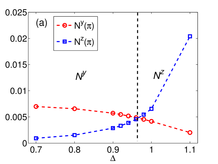
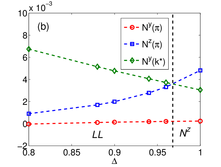
Figure S1: (Color online) Order parameters $N^{y}(\pi)$ (red circles), $N^{z}(\pi)$ (blue squares) and $N^{y}(k^{*})$ (green diamonds) extrapolated by a second order polynomial (17) using data from $L=600$, $800$, $1000$, $1200$, and $1600$ chains as a function of $\Delta$ at (a) $h/J=0.2$ and (b) $h/J=0.05$ with $D/J=0.1$. The crossing points of the order parameters determine the phase boundary.

In this appendix, we provide details on the determination of the phase diagram and finite-size effects.

F.1 Determination of phase boundaries

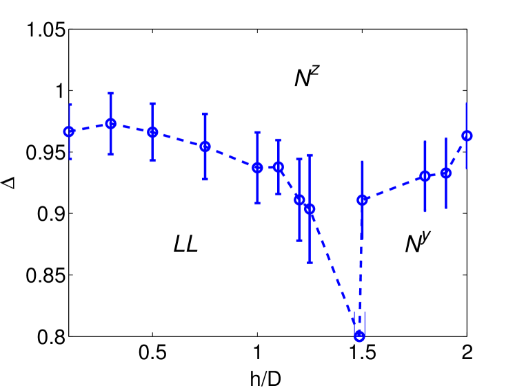
Figure S2: (Color online) Phase diagram of the chain with $D/J=0.1$ after the finite-size extrapolation of the order parameters to $L=\infty$ using Eq.(17). The error bar are plotted at the 95% confidence interval of the order parameters.

Here we describe how we determine phase boundaries numerically. In Fig. S1(a) we show the extrapolated order parameters at $k=\pi$ near the phase boundary between the $N^{y}$ and $N^{z}$ phases. Here we can see that these two distinct orders are dominant in the corresponding phases, hence the phase boundary between them can be determined by their crossing point.

Figure S1(b) shows the order parameters near the boundary between the LL and $N^{z}$ phases, where both order parameters $N^{y}(k=k^{*})$ and $N^{z}(k=\pi)$ are finite and dominant on the opposite sides of the figure, while $N^{y}(k=\pi)$ is vanishingly small. Notice that due to large finite-size effect, the order parameter $N^{y}(k=k^{*})$, which should vanish after extrapolation to the thermodynamic limit $L\to\infty$, still remains finite in our $L=1600$ chain, although rather small. As a result, we use it to identify the LL phase as described in the main text.

F.2 Finite size effects on the phase boundary

To check the finite-size effect on phase boundaries, we have compared phase diagrams for the chain of length $L=1200$ calculated by DMRG and iTEBD methods as shown in Fig. 4. To minimize the boundary effect, the order parameters are calculated within the central half of the system, i.e., 600 sites in the middle of the system. We keep the same bond-link dimension and considering the same lengths for the calculation of correlation functions using iTEBD and DMRG methods. The agreement between the DMRG and iTEBD results is quite good, suggesting that the DMRG results are only subject to the finite size effect while the effect of open boundaries is negligible.

Figure S2 shows the phase diagram obtained by extrapolating order parameters to $L=\infty$ using second-order polynomial functions of $1/\sqrt{L}$ [Eq. (17)]. Comparing it to the phase diagram in Fig. 4 for the finite system of size $L=1200$, we observe the shift of the $N^{z}$-$LL$ and $N^{z}$-$N^{y}$ boundaries to slightly larger $\Delta$ values. A more detailed analysis suggests that error bars associated with the finite-size extrapolation to $L=\infty$ are within a 95% confidence interval, which means that our conclusion about the $N^{z}$ Ising order extending to the $\Delta<1$ region is well justified.

It is also possible to determine the phase boundary by computing the Binder cumulantPelissetto and Vicari (2002); West et al. (2015); Saadatmand et al. (2015), which is widely used in Monte Carlo studies and has also been recently applied in the DMRG study West et al. (2015); Saadatmand et al. (2015). Our preliminary investigation suggests that the phase boundary determined with the help of the Binder cumulant is fully consistent with the results obtained in this work.

References

- Alicea (2012) J. Alicea, Reports on Progress in Physics 75, 076501 (2012), URL http://stacks.iop.org/0034-4885/75/i=7/a=076501.
- Manchon et al. (2015) A. Manchon, H. C. Koo, J. Nitta, S. M. Frolov, and R. A. Duine, Nat Mater 14, 871 (2015), ISSN 1476-1122, review, URL http://dx.doi.org/10.1038/nmat4360.
- Kitaev (2001) A. Y. Kitaev, Physics-Uspekhi 44, 131 (2001), URL http://stacks.iop.org/1063-7869/44/i=10S/a=S29.
- Kitaev (2006) A. Kitaev, Annals of Physics (N.Y.) 321, 2 (2006), ISSN 0003-4916, january Special Issue.
- Dzyaloshinskii (1958) I. E. Dzyaloshinskii, Journal of Physics and Chemistry of Solids 4, 241 (1958), ISSN 0022-3697, URL http://www.sciencedirect.com/science/article/pii/0022369758900763.
- Moriya (1960) T. Moriya, Phys. Rev. 120, 91 (1960), URL https://link.aps.org/doi/10.1103/PhysRev.120.91.
- Dzyaloshinskii (1965) I. E. Dzyaloshinskii, Zh. Eksp. Teor. Fiz. 47, 992 (1964) [Sov. Phys. - JETP 20, 665] (1965).
- Zheludev et al. (1998) A. Zheludev, S. Maslov, G. Shirane, Y. Sasago, N. Koide, and K. Uchinokura, Phys. Rev. B 57, 2968 (1998), URL https://link.aps.org/doi/10.1103/PhysRevB.57.2968.
- Togawa et al. (2012) Y. Togawa, T. Koyama, K. Takayanagi, S. Mori, Y. Kousaka, J. Akimitsu, S. Nishihara, K. Inoue, A. S. Ovchinnikov, and J. Kishine, Phys. Rev. Lett. 108, 107202 (2012), URL https://link.aps.org/doi/10.1103/PhysRevLett.108.107202.
- Cheong and Mostovoy (2007) S.-W. Cheong and M. Mostovoy, Nat Mater 6, 13 (2007), ISSN 1476-1122, URL http://dx.doi.org/10.1038/nmat1804.
- Kishine and Ovchinnikov (2015) J. Kishine and A. Ovchinnikov, Solid State Physics 66, 1 (2015), ISSN 0081-1947, URL http://www.sciencedirect.com/science/article/pii/S0081194715000041.
- Povarov et al. (2011) K. Y. Povarov, A. I. Smirnov, O. A. Starykh, S. V. Petrov, and A. Y. Shapiro, Phys. Rev. Lett. 107, 037204 (2011), URL https://link.aps.org/doi/10.1103/PhysRevLett.107.037204.
- Hälg et al. (2014) M. Hälg, W. E. A. Lorenz, K. Y. Povarov, M. Månsson, Y. Skourski, and A. Zheludev, Phys. Rev. B 90, 174413 (2014), URL http://link.aps.org/doi/10.1103/PhysRevB.90.174413.
- Smirnov et al. (2015) A. I. Smirnov, T. A. Soldatov, K. Y. Povarov, M. Hälg, W. E. A. Lorenz, and A. Zheludev, Phys. Rev. B 92, 134417 (2015), URL http://link.aps.org/doi/10.1103/PhysRevB.92.134417.
- Gangadharaiah et al. (2008) S. Gangadharaiah, J. Sun, and O. A. Starykh, Phys. Rev. B 78, 054436 (2008), URL http://link.aps.org/doi/10.1103/PhysRevB.78.054436.
- Garate and Affleck (2010) I. Garate and I. Affleck, Phys. Rev. B 81, 144419 (2010), URL http://link.aps.org/doi/10.1103/PhysRevB.81.144419.
- Sun and Pokrovsky (2015) C. Sun and V. L. Pokrovsky, Phys. Rev. B 91, 161305 (2015), URL https://link.aps.org/doi/10.1103/PhysRevB.91.161305.
- Dmitrienko et al. (2014) V. E. Dmitrienko, E. N. Ovchinnikova, S. P. Collins, G. Nisbet, G. Beutier, Y. O. Kvashnin, V. V. Mazurenko, A. I. Lichtenstein, and M. I. Katsnelson, Nat Phys 10, 202 (2014), ISSN 1745-2473.
- Schnyder et al. (2008) A. P. Schnyder, O. A. Starykh, and L. Balents, Phys. Rev. B 78, 174420 (2008), URL http://link.aps.org/doi/10.1103/PhysRevB.78.174420.
- Jin and Starykh (2017) W. Jin and O. A. Starykh, Phys. Rev. B 95, 214404 (2017), URL https://link.aps.org/doi/10.1103/PhysRevB.95.214404.
- Fradkin (2013) E. Fradkin, Field Theories of Condensed Matter Physics (Cambridge University Press, Cambridge, 2013), ISBN 9781139015509, cambridge Books Online, URL http://dx.doi.org/10.1017/CBO9781139015509.
- Starykh et al. (2005) O. A. Starykh, A. Furusaki, and L. Balents, Phys. Rev. B 72, 094416 (2005), URL http://link.aps.org/doi/10.1103/PhysRevB.72.094416.
- Giamarchi and Schulz (1988) T. Giamarchi and H. Schulz, Journal de Physique 49, 819 (1988), URL https://hal.archives-ouvertes.fr/jpa-00210759.
- Dmitriev et al. (2002) D. V. Dmitriev, V. Y. Krivnov, and A. A. Ovchinnikov, Phys. Rev. B 65, 172409 (2002), URL http://link.aps.org/doi/10.1103/PhysRevB.65.172409.
- White (1992) S. R. White, Phys. Rev. Lett. 69, 2863 (1992), URL http://link.aps.org/doi/10.1103/PhysRevLett.69.2863.
- White (1993) S. R. White, Phys. Rev. B 48, 10345 (1993), URL http://link.aps.org/doi/10.1103/PhysRevB.48.10345.
- Schollwöck (2005) U. Schollwöck, Rev. Mod. Phys. 77, 259 (2005), URL http://link.aps.org/doi/10.1103/RevModPhys.77.259.
- Vidal (2003) G. Vidal, Phys. Rev. Lett. 91, 147902 (2003), URL http://link.aps.org/doi/10.1103/PhysRevLett.91.147902.
- Vidal (2004) G. Vidal, Phys. Rev. Lett. 93, 040502 (2004), URL http://link.aps.org/doi/10.1103/PhysRevLett.93.040502.
- Vidal (2007) G. Vidal, Phys. Rev. Lett. 98, 070201 (2007), URL http://link.aps.org/doi/10.1103/PhysRevLett.98.070201.
- Starykh (2010) O. A. Starykh, in Handbook of Nanophysics: Nanotubes and Nanowires, edited by K. D. Sattler (CRC, Boca Raton, 2010), chap. 30.
- Lukyanov and Zamolodchikov (1997) S. Lukyanov and A. Zamolodchikov, Nuclear Physics B 493, 571 (1997), ISSN 0550-3213, URL http://www.sciencedirect.com/science/article/pii/S0550321397001235.
- Hikihara and Furusaki (1998) T. Hikihara and A. Furusaki, Phys. Rev. B 58, R583 (1998), URL https://link.aps.org/doi/10.1103/PhysRevB.58.R583.
- Hikihara and Furusaki (2004) T. Hikihara and A. Furusaki, Phys. Rev. B 69, 064427 (2004), URL https://link.aps.org/doi/10.1103/PhysRevB.69.064427.
- Hikihara et al. (2017) T. Hikihara, A. Furusaki, and S. Lukyanov, Phys. Rev. B 96, 134429 (2017).
- Pelissetto and Vicari (2002) A. Pelissetto and E. Vicari, Physics Reports 368, 549 (2002), ISSN 0370-1573, URL http://www.sciencedirect.com/science/article/pii/S0370157302002193.
- West et al. (2015) C. G. West, A. Garcia-Saez, and T.-C. Wei, Phys. Rev. B 92, 115103 (2015), URL https://link.aps.org/doi/10.1103/PhysRevB.92.115103.
- Saadatmand et al. (2015) S. N. Saadatmand, B. J. Powell, and I. P. McCulloch, Phys. Rev. B 91, 245119 (2015), URL https://link.aps.org/doi/10.1103/PhysRevB.91.245119.