Formation and Reconnection of Three-dimensional Current Sheets with a Guide Field in the Solar Corona

Abstract

We analyze a series of three-dimensional magnetohydrodynamic numerical simulations of magnetic reconnection in a model solar corona to study the effect of the guide field component on quasi-steady state interchange reconnection in a pseudostreamer arcade configuration. This work extends the analysis of Edmondson et al. (2010b) by quantifying the mass density enhancement coherency scale in the current sheet associated with magnetic island formation during the nonlinear phase of plasmoid-unstable reconnection. We compare the results of four simulations of a zero, weak, moderate, and a strong guide field, $B_{GF}/B_{0}=\{0.0,0.1,0.5,1.0\}$, to quantify the plasmoid density enhancement’s longitudinal and transverse coherency scales as a function of the guide field strength. We derive these coherency scales from autocorrelation and wavelet analyses, and demonstrate how these scales may be used to interpret the density enhancement fluctuation’s Fourier power spectra in terms of a structure formation range, an energy continuation range, and an inertial range—each population with a distinct spectral slope. We discuss the simulation results in the context of solar and heliospheric observations of pseudostreamer solar wind outflow and possible signatures of reconnection-generated structure.

=4

1 Introduction

Magnetic reconnection is one of the most interesting and fundamental plasma physics processes of mass, momentum, and energy transfer observed in geophysical, astrophysical, and laboratory plasmas (see reviews by Zweibel & Yamada, 2009; Pontin, 2011; Daughton & Roytershteyn, 2012, and references therein). Since the introduction of the fractal reconnection interpretation by Shibata & Tanuma (2001) of the well-known tearing-mode (Furth et al., 1963; Biskamp, 1986), there has been significant advances in theoretical and numerical simulation work examining the dynamics and evolution of resistive tearing and magnetic island creation, now often referred to as the plasmoid instability, including the formation and subsequent fragmentation of secondary current sheets during the system’s transition to fully nonlinear evolution (e.g. Loureiro et al., 2007, 2012; Lapenta, 2008; Huang & Bhattacharjee, 2010; Uzdensky et al., 2010; Bárta et al., 2011; Murphy et al., 2013; Pucci & Velli, 2014; Tenerani et al., 2016). In three-dimensions (3D), the additional degree of freedom allows for a much broader range of dynamics available to the system undergoing reconnection—everything from the interaction of magnetic flux ropes (Linton et al., 2001; Linton & Priest, 2003), the role of the guide field on particle and field evolution in and around the diffusion region (Pritchett & Coroniti, 2004; Karimabadi et al., 2005; Drake et al., 2006, 2014), to the macroscopic evolution of 3D tearing and reconnection along the current sheet (e.g. Linton et al., 2009; Shimizu et al., 2009; Shepherd & Cassak, 2012; Cassak et al., 2013), and the development of turbulence as a result of the reconnection itself (see review by Karimabadi & Lazarian, 2013, and references therein).

Nishida et al. (2013) examined the formation of 3D magnetic island plasmoids in an eruptive flare current sheet and Wyper & Pontin (2014a; 2014b) have shown the evolution of magnetic island flux rope structures can result in exceedingly complex dynamics, even when the 3D islands are more-or-less confined to a quasi-2D surface or within adjacent boundary layers. Additionally, Baalrud et al. (2012) have shown that in 3D, the unstable modes of the plasmoid instability can grow at oblique angles which can interact and lead to a kind of “self-generated” turbulent reconnection (e.g. Oishi et al., 2015; Huang & Bhattacharjee, 2016) and Wang et al. (2015) have shown that the efficiency of magnetic energy conversion in 3D MHD reconnection is increased by similar nonlinear coupling between the inflow and outflow regions of multiple tearing layers that form in a global current sheet.

Edmondson et al. (2010b) showed the self-consistent formation and evolution of (very short) three-dimensional plasmoidal flux ropes within a singular reconnection current sheet in MHD. While this system exhibited turbulent characteristics, the effect of the plasmoids on the evolution of the system, however, could not be addressed. Several kinetic studies of three-dimensional reconnection layers in anti-parallel and finite guide field geometries have shown the evolution is always dominated by the formation and interaction of secondary islands (Daughton et al., 2011a, b). The flux ropes are produced by secondary instabilities within the electron layers, occur in both collisional regimes and large-scale collisionless systems, and lead to turbulent evolution. In particular, in the collisional regime the secondary islands break the Sweet-Parker scaling rate driving the system to kinetically-dominated scales.

Recently, Fujimoto (2016) highlighted the intermittent, quasi-turbulent formation and ejection of 3D magnetic island plasmoid flux ropes in a particle-in-cell simulation, obtaining results that are qualitatively similar to the MHD simulation results we present here. Analysis of magnetic reconnection processes at MHD scales is valuable specifically because of the intrinsic coupling of disparate spatial scales associated with the diffusion region and the macroscopic evolution of global system in which the both large-scale magnetic field and bulk plasma dynamics directly influence the reconnection process. The most obvious example of this intrinsic scale-coupling in the corona is in solar flares (e.g. see Janvier, 2017, and references therein), however, there is mounting evidence that magnetic reconnection processes are also likely to be important to the origin of the slow solar wind.

The basic, steady-state picture of slow solar wind generation from coronal helmet streamers and pseudostreamers has been established (e.g. Sheeley et al., 1999; Wang et al., 2000, 2012; Riley & Luhmann, 2012). The static (i.e., potential) magnetic field structure of coronal pseudostreamers is expected to produce a stationary slow wind due to the flux tube expansion factors (Arge & Pizzo, 2000; Cranmer, 2012; Wang et al., 2012). A prediction of the Separatrix-Web model (Antiochos et al., 2011, 2012; Titov et al., 2012) is that pseudostreamer slow wind forms along arcs that can extend large angular distances away from the main helmet streamer belt and recent in situ data analysis appear to confirm this scenario (Crooker et al., 2012, 2014; Owens et al., 2014).

In situ observations of slow solar wind plasma, field, and composition and their variability—including during periods of pseudostreamer wind—are strongly suggestive of a closed-field coronal source region which implies some magnetic reconnection process as a crucial component of its origin (Zurbuchen et al., 2000, 2002; Kepko et al., 2016). Higginson et al. (2017c) have demonstrated that the 3D structure of reconnection-generated magnetic islands in the heliospheric current sheet are consistent with the observations of small-scale flux rope transients in the slow solar wind (Feng et al., 2008; Cartwright & Moldwin, 2008, 2010; Kilpua et al., 2009; Yu et al., 2014). And Janvier et al. (2014) have argued that the power-law distribution of the sizes of these small flux rope transients appears compatible with the power-law distributions of magnetic island plasmoids obtained in various reconnection studies (e.g. Uzdensky et al., 2010; Fermo et al., 2010; Huang & Bhattacharjee, 2012; Loureiro et al., 2012; Shen et al., 2013; Lynch et al., 2016).

The magnetic topology of a pseudostreamer is a region of opposite polarity embedded in unipolar field (e.g., Edmondson et al., 2009, 2010a; Lynch et al., 2016). The bipolar, closed-flux system has a magnetic null point and separatrix dome defining the boundary between the closed and open flux systems at low-to-moderate heights in the atmosphere (Wang et al., 2007, 2012; Titov et al., 2012; Rachmeler et al., 2014). We, and many other researchers, have shown that this pseudostreamer topology is ideally suited for the formation of current sheets and magnetic reconnection in response to global stresses accumulated via photospheric motions or other gradual energization processes (e.g., see Masson et al., 2014, and references therein). Thus, interchange reconnection as a dynamic and transient release mechanism of previously closed-flux plasma into the open field continues to be explored in remote sensing observations and in numerical simulations (Baker et al., 2009; Edmondson et al., 2010a; van Driel-Gesztelyi et al., 2012; Rappazzo et al., 2012; Masson et al., 2012, 2014; Lynch et al., 2014; Pontin & Wyper, 2015; Viall & Vourlidas, 2015; Higginson et al., 2017a, b).

Here we present an extension of the Edmondson et al. (2010b) investigation, hereafter referred to as Paper I, by performing a set of new high-resolution, adaptively-refined 3D MHD simulations with a systematically increasing guide field component to examine the role of the guide field on the development and evolution of the reconnection. Our simulations start from a true 3D magnetic null line (X-type null point in 2D cross-section) and follow the formation and evolution of the current sheet in response to global driving far from the magnetic null line. Thus, our current sheet formation and reconnection are a self-consistent response to the imposed separation of the pseudostreamer arcade spine lines (fan surfaces) in the Syrovatskii scenario (Syrovatskii, 1978a, b, 1981; Antiochos et al., 2002).

The paper is organized as follows. In section 2, we describe the numerical methods, the magnetic configurations, and boundary conditions for our set of MHD simulations. In section 3, we present our simulation results including the transition to the non-linear phase of the plasma instability under “steady state” reconnection ($\S$ 3.1), the effects of the guide field on the characteristics of 3D plasmoid magnetic island flux ropes ($\S$ 3.2), and the quantitative comparison of the coherency scales of the reconnection-generated plasmoid densities in each of the current sheets ($\S$ 3.3). In section 4, we discuss our results in terms of reconnection-generated solar wind outflow at psuedostreamers and in section 5, we present our conclusions.

2 Numerical Simulations

We use the Adaptively Refined MHD Solver (ARMS; DeVore & Antiochos, 2008) to solve the ideal MHD equations in Cartesian coordinates,

$$\frac{\partial\rho}{\partial t}+\nabla\cdot\left(\ \rho\ \bm{V}\ \right)=0\ ,$$ (1)

$$\frac{\partial\left(\ \rho\ \bm{V}\ \right)}{\partial t}+\nabla\cdot\left(\ \rho\ \bm{V}\ \bm{V}\ \right)+\nabla P=\frac{1}{4\pi}\ \left(\ \nabla\times\bm{B}\ \right)\times\bm{B}\ ,$$ (2)

$$\frac{\partial T}{\partial t}+\nabla\cdot\left(\ T\ \bm{V}\ \right)+\left(\ 1-\gamma\ \right)\ T\ \left(\ \nabla\cdot\bm{V}\ \right)=0\ ,$$ (3)

$$\frac{\partial\bm{B}}{\partial t}=\nabla\times\left(\ \bm{V}\times\bm{B}\ \right)\ .$$ (4)

The variables retain their usual meaning: mass density $\rho$, velocity vector $\bm{V}$, magnetic field vector $\bm{B}$, and we have written the energy equation in terms of the plasma temperature $T$. The ratio of specific heats is $\gamma=5/3$. The system is closed with the ideal gas law,

$$P=2\left(\frac{\rho}{m_{p}}\right)k_{B}T\ ,$$ (5)

where $m_{p}$ is the mass of a proton and $k_{B}$ is the Boltzmann constant.

ARMS utilizes block-adaptive computational gridding based on the PARAMESH toolkit (MacNeice et al., 2000) for static and dynamic grid refinement and is optimized for modern massively parallel supercomputing architectures. ARMS has been used to study numerous dynamic phenomena in the solar atmosphere, including coronal jets (Pariat et al., 2015; Wyper et al., 2016; Karpen et al., 2017), theinteraction between closed and open fields at streamer boundaries (Edmondson et al., 2009, 2010a; Masson et al., 2013; Higginson et al., 2017a, b), and the examination of plasmoid-unstable reconnection and magnetic island evolution (Paper I; Guidoni et al. 2016; Lynch et al. 2016).

2.1 Initial Configuration, Driving Flows, and Boundary Conditions

The initial model atmosphere consists of a uniform mass density, $\rho_{0}=1.6726\times 10^{-16}$ g cm^-3, and pressure, $P_{0}=0.035$ dyne cm^-2, that result in an initial uniform temperature of $T_{0}=1.27\times 10^{6}$ K. The initial magnetic field configuration is a pseudostreamer arcade embedded in a uniform vertical background field (e.g., Paper I; Lynch & Edmondson 2013). The background field strength is $B_{0}=3.0$ G. The characteristic plasma beta is $\beta_{0}\equiv 8\pi P_{0}/B_{0}^{2}=0.1$, and characteristic Alfvén speed $V_{A0}\equiv B_{0}/\sqrt{4\pi\rho_{0}}=650$ km s^-1. The characteristic length scale is $L_{0}=10^{9}$ cm, which yields a characteristic Alfvén time of $\tau_{A0}\equiv L_{0}/V_{A0}=15.385$ s. Furthermore, we define a characteristic current density magnitude, $J_{0}=(c/4\pi)\ B_{0}/L_{0}=7.162$ statamp cm^-2.

We investigate the effect of increasing the guide field strength on the self-consistent current sheet formation, evolution, and magnetic reconnection dynamics. We define a guide field factor normalized to the uniform background field strength, $\zeta\equiv B_{GF}/B_{0}$, and use this notation to describe, respectively, the zero ($\zeta=0.0$), weak ($\zeta=0.1$), moderate ($\zeta=0.5$), and strong ($\zeta=1.0$) guide field cases. The $\zeta$ parameter spans the transition from strictly anti-parallel reconnection to component reconnection, i.e., $\zeta=\tan\left(\phi\right)$ for relative alignment angles of $\phi=\{0^{\circ},5.7^{\circ},26.6^{\circ},45^{\circ}\}$. We note the variation in the guide field leads to variations in the respective system characteristics for each simulation: plasma beta $\beta_{\zeta}=\beta_{0}\left(\ 1+\zeta^{2}\ \right)^{-1}$, Alfvén speed $V_{A\zeta}=V_{A0}\left(\ 1+\zeta^{2}\ \right)^{1/2}$, and Alfvén time $\tau_{A\zeta}=\tau_{A0}\left(\ 1+\zeta^{2}\ \right)^{-1/2}$.

The initial embedded pseudostreamer model is a translationally symmetric magnetic field, constructed from a the vector potential of the form

$$\bm{A}_{\zeta}=zB_{0}\left(\ \bm{\hat{x}}-\zeta\ \bm{\hat{y}}\ \right)+A_{z}(x,y)\ \bm{\hat{z}}\ .$$ (6)

For all $\zeta$, the initial vector magnetic field $\bm{B}_{\zeta}=\nabla\times\bm{A}_{\zeta}$ is clearly independent of $z$. Furthermore, the underlying pseudostreamer model is constructed from the vector potential of a series of line dipoles at positions $\bm{r}_{n}=\pm nd\ \bm{\hat{x}}$,

$$A_{z}(x,y)=M_{0}\ \sum_{n=0}^{N}\ \frac{\left(\ \left(x\pm nd\right)/L_{0}\ \right)}{\left(\ \left(x\pm nd\right)/L_{0}\ \right)^{2}+\left(\ y/L_{0}\ \right)^{2}}\ .$$ (7)

The linear-dipole strength is set $M_{0}=-40$ G cm in order to produce a $B_{y}$ value of -25 G at the lower boundary of $y=1.0L_{0}$ in the pseudostreamer arcades. The dipole spacing length, $d=15L_{0}$, means the contributions of the line dipoles exactly cancel at $x=\pm nd/2$ for an infinite series (and are effectively zero when the series is truncated at $N=25$, see Paper I for details). Figure 1 shows an isometric perspective of the magnetic field structure for the $\zeta=0.1$ (left panel) and $\zeta=1.0$ (right panel) simulations at $t=0$ which illustrates the tilt added in the $z$-direction by the guide field component. The closed pseudostreamer arcade flux systems are indicated by yellow and red field lines whereas the external unipolar open flux system is represented by blue and green field lines. The internal spine line (fan surface) is between the yellow and red flux systems whereas the external spine line (fan surface) is between the blue and green flux systems. Figure 2(a) shows the 2D $x$-$y$ projection of these flux systems which are identical in each simulation.

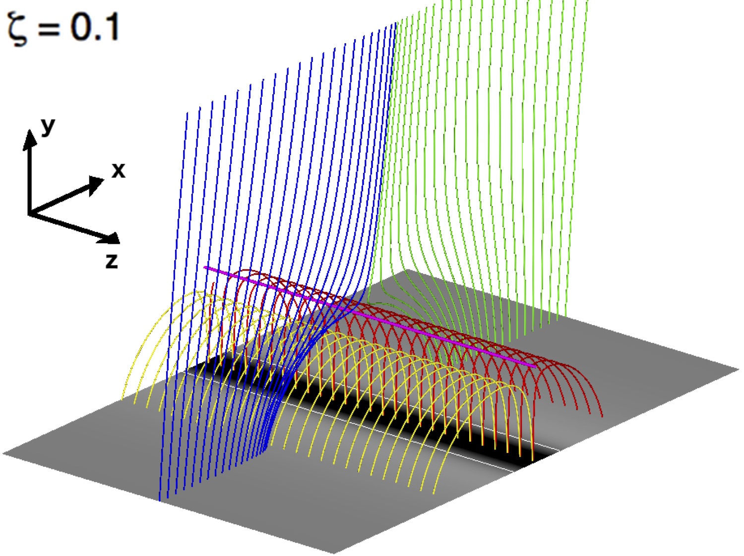
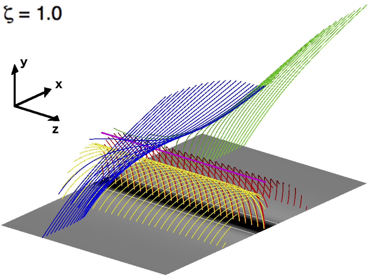
Figure 1: Representative field lines at $t=0$ s showing the initial 3D magnetic configuration of our translationally symmetric pseudostreamer arcade for weak ($\zeta=0.1$, left panel) and strong ($\zeta=1.0$, right panel) guide field components. The $y=1$ surface shows the normal magnetic field component $B_{y}(x,z)$ in grayscale at the lower boundary and the polarity inversion lines are shown as the thin white lines under each arcade. The thick magenta field line indicates the X-point null line.

The system is energized in two stages with a spatially-uniform flow applied at the upper boundary, a distance of approximately 7$L_{0}$ away from the X-point. The first stage is a smooth acceleration phase followed by a constant flow for the duration of the simulations. The boundary flow is given by $\bm{V}_{\rm{flow}}=0.015V_{A0}\ T(t)\ \hat{\bm{x}}$, where $T(t)$ is a piecewise-continuous, dimensionless function defined by $T(t)=1-\cos{\left(\pi t/\left(65\ \tau_{A0}\right)\right)}$ for $0\leq t\leq 65\ \tau_{A0}$ and $T(t)=1$ for $t>65\ \tau_{A0}$. This corresponds to a uniform driving flow of $V_{0}=20$ km s^-1 for $t\geq 10^{3}$ s. We note that while the boundary flows are greater than typically observed photospheric velocities ($\sim$1 km s^-1), our boundary flows remain extremely sub-Alfvénic ($M_{A}\sim 0.03$) and sub-sonic ($M_{s}\sim 0.10$).

We employ periodic boundary conditions in the $x$- and $z$-boundaries of our Cartesian domain. In addition, we set extrapolative and zero-gradient boundary conditions at the upper and lower $y$-surfaces. Furthermore, we fix the lower $y$-boundary to no slip and reflecting. Despite the periodicity in the $x$- and $z$-boundary conditions, we achieve a quasi-steady state response such that the inflows at the reconnection layer reach an asymptotic value dictated by the constant boundary driving boundary flow.

2.2 Computational Grid, Adaptive Mesh Refinement, & Numerical Resistivity

The computational domain is $x/L_{0}\in\left[\ -7.5,7.5\ \right]$, $y/L_{0}\in\left[\ 1.0,11.0\ \right]$, and $z/L_{0}\in\left[\ -5.0,5.0\ \right]$. The computational grid is comprised of $3\times 2\times 2$ root blocks with $8^{3}$ grid cells per block. There are 6 levels of static grid refinement and two additional levels of dynamic refinement. The maximum level 8 grid resolution corresponds to an effective resolution of $3072\times 2048\times 2048$ and is equivalent to the spatial resolution used in Paper I. The length of the computational grid cell in the highest-refinement region is thus $\delta=10L_{0}/2048=4.883\times 10^{6}$ cm.

Figure 2 panel (a) shows the root block structure of the static grid over the full domain at $t=0$ with representative magnetic field lines colored as in Figure 1. The static grid structure is translationally symmetric through all $z=$ constant planes, for all $\zeta$ simulations. The adaptive mesh refinement (AMR) is conditional to the current density magnitude $|J|$. We fix the non-dimensional AMR refinement, $J_{l}/J_{0}$, and derefinement, $J_{r}/J_{0}$, thresholds to $7.0\times 10^{-7}$ and $4.2$, respectively.

Figure 2 panel (b) shows the current density magnitude $|J|$ in grayscale through the $z=0$ plane at $t=104\ t_{A0}$ for the no guide-field $\zeta=0$ case. The dynamic grid refinement region is concentrated at the current sheet where the blue and red magnetic flux is reconnecting to become part of the yellow and green flux systems.

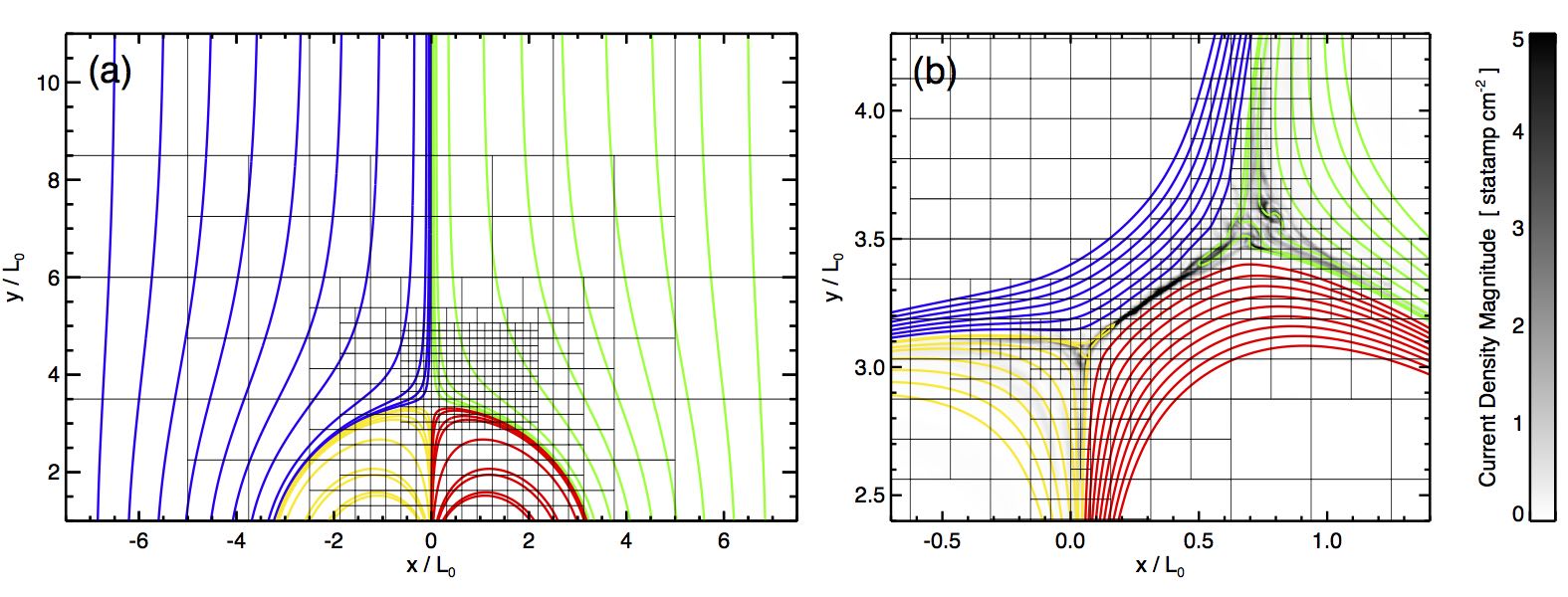
Figure 2: (a) Block structure of the six levels of static grid refinement through all $z=$ constant planes (with representative magnetic field lines at $t=0$). (b) Current density magnitude $|J|$ through the $z=0$ plane at $t=104\tau_{A0}$ in simulation $\zeta=0$ showing the two additional levels of dynamic block refinement.

We solve the equations of ideal MHD without an explicit, physical magnetic resistivity. However, necessary and stabilizing numerical diffusion terms introduce an effective viscosity and resistivity on very small spatial scales. In this way, magnetic reconnection occurs when the large magnetic field gradients associated with current sheet features become under-resolved, i.e., have been compressed to the local grid resolution scale. One usually estimates the effective numerical resistivity by balancing the average inflow timescale of magnetic flux into the current sheet (of thickness $\delta$) against the resistive dissipation timescale,

$$\eta\sim\delta\ \langle\ V_{in}\ \rangle\ .$$ (8)

We note that Equation (8) is a simple balance between the ideal transverse and dissipation timescales, and therefore should be considered an over-estimate of the actual numerical resistivity. For ARMS, and finite-volume FCT schemes in general, the numerical resistivity is a local quantity that depends explicitly on the gradients of the field and flows used to determine how much of the higher-order anti-diffusion correction is applied to the lower-order diffusive transport (DeVore, 1991). While Equation (8) is the estimate typically used in MHD simulations there remains a question as to why many numerical simulations with Lundquist numbers of a few $\times 10^{3}$ (e.g. Paper I; Ni et al. 2010; Shen et al. 2011; Lynch et al. 2016), exhibit nonlinear dynamics and plasmoid-unstable evolution similar to those simulations with higher Lundquist numbers that exceed the more traditional $\gtrsim 10^{4}$ threshold (e.g. Furth et al., 1963; Biskamp, 1986; Huang & Bhattacharjee, 2010; Loureiro et al., 2012; Murphy et al., 2013).

In Appendix A, we derive corrections to the Equation (8) numerical resistivity estimate based on the transport of total energy density through the current sheet to obtain

$$\eta\sim\delta\ \langle\ V_{in}\ \rangle\ \frac{\left(\ \chi+Z\ \right)}{4},$$ (9)

where the dimensionless factors $\chi$ and $Z$ describe the advection of magnetic energy density and plasma compressibility, respectively. To first order in the current sheet aspect ratio $\delta/\langle\ L_{CS}\ \rangle$,

$$\chi\equiv 1-\left(\ 2\ \frac{\langle\ B_{out}\ \rangle}{\langle\ B_{in}\ \rangle}+\frac{\langle\ V_{out}\ \rangle}{\langle\ V_{in}\ \rangle}\ \frac{\mathcal{ME}_{out}}{\mathcal{ME}_{in}}\ \right)\frac{\delta}{\langle\ L_{CS}\ \rangle}\ ,$$ (10)

$$Z\equiv M_{Ain}^{2}\left[\ 1-\left(\ 2\ \frac{\langle\ B_{out}\ \rangle}{\langle\ B_{in}\ \rangle}+\frac{\langle\ V_{out}\ \rangle}{\langle\ V_{in}\ \rangle}\ \frac{\mathcal{KE}_{out}}{\mathcal{KE}_{in}}\ \right)\frac{\delta}{\langle\ L_{CS}\ \rangle}\ \right]\ .$$ (11)

The brackets signify an appropriate spatial-averaging procedure, such that $\mathcal{ME}=\langle\ B\ \rangle^{2}/(8\pi)$ and $\mathcal{KE}=\langle\ \rho\ \rangle\langle\ V\ \rangle^{2}/2$ are the respective magnetic and kinetic energy densities advected with the inflows and outflows, and $M_{Ain}=\langle\ V_{in}\ \rangle/\langle\ V_{Ain}\ \rangle$ is the Alfvénic Mach number of the inflow. From Equation (9), one sees immediately that the traditional $\eta\sim\delta\ \langle\ V_{in}\ \rangle$ numerical resistivity estimate could be overestimated by up to a factor of 4 in the thin current sheet, incompressible (low Alfvénic Mach number) inflow limit ($\chi\rightarrow 1$, $Z\rightarrow 0$).

3 Simulation Results

The basic evolution of our system is that of driven reconnection in which the reconnection inflow speed adjusts in an attempt to achieve a quasi-steady state where the rate of material and flux processed through the current sheet is determined by the distant boundary driving flows. For very slow driving, the reconnection is essentially the Sweet-Parker type and the current sheet remains laminar in the sense of a quasi-static, reversible thermodynamic process. As the driving increases, the system attempts to process more material and flux through the current sheet and the reconnection rate necessarily increases. Once the rate of material and magnetic flux to process exceeds the current sheet’s capacity via the Sweet-Parker type reconnection, basic mass and energy continuity necessitate the rapid onset of nonlinearity and the development of plasmoid-unstable evolution (see also Daughton et al., 2011a, b; Pucci & Velli, 2014; Tenerani et al., 2016).

3.1 Onset of the Non-Linear Phase of the Plasmoid Instability

The driving flows at the upper boundary increases the magnetic energy such that the material and flux are being processed/transferred through the current sheet at the same rate. Magnetic flux is transferred so as to spread the volumetric (force-free) currents into as large a volume as possible. For relatively weak guide field cases, the magnetic energy is (marginally) reduced as flux is processed through the current sheet and transferred between domains; that is until the overlying field becomes stretched enough to saturate this effect throughout the entire box. Increasing the guide field has the effect of suppressing this process/transfer effect through the current sheet. In other words, a stronger guide field smooths the magnetic field gradients which delays the onset of nonlinear dynamics. We note this system is not undergoing free-reconnection, but rather, the reconnection dynamics are driven in a well-controlled quasi-steady state manner such that the inflow Alfvénic Mach number matches that of the driving flows at the boundary.

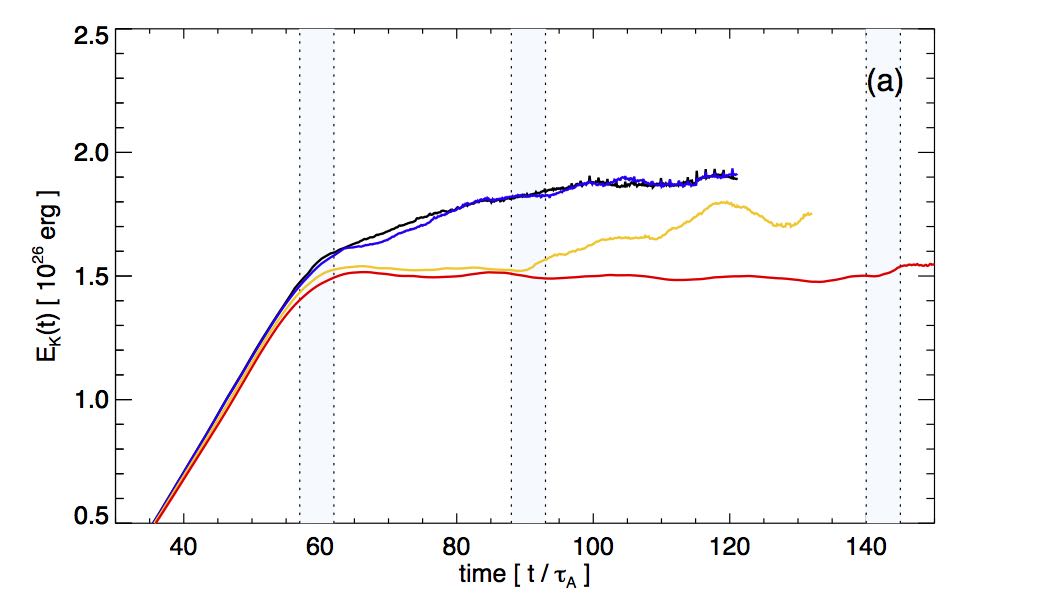
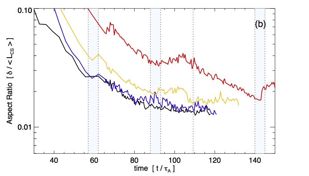
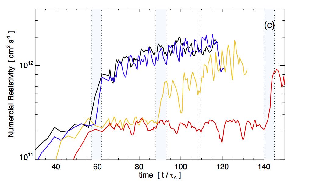
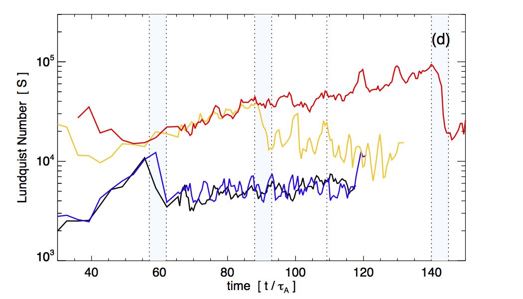
Figure 3: (a) Kinetic energy evolution. (b) Current sheet aspect ratio evolution. (c) Numerical resistivity evolution. (d) Lundquist number evolution. Every panel shows the four different guide field simulations: black is $\zeta=0.0$, blue is $\zeta=0.1$, yellow is $\zeta=0.5$, and red is $\zeta=1.0$. Vertical blue stripes indicate the onset of nonlinear evolution and the plasmoid instability.

The delay in the onset of the nonlinear reconnection phase can be seen in Figure 3(a) which shows the global kinetic energy in the simulation domains for all four simulations: $\zeta=0.0$ (black), $\zeta=0.1$ (blue), $\zeta=0.5$ (yellow), and $\zeta=1.0$ (red). The total kinetic energy of the uniform driving at the upper boundary can be seen to be approximately $1.5\times 10^{26}$ erg. Any additional kinetic energy is associated with the plasmoid-unstable reconnection dynamics and relatively fast reconnection jet outflow. The zero and weak, $\zeta=0.0$ and $0.1$, guide field cases (black, blue lines) immediately transition into the nonlinear phase by $t/\tau_{A}\gtrsim 56$. The moderate, $\zeta=0.5$, guide field simulation (yellow line) begins this transition by $t/\tau_{A}\gtrsim 88$ and the strong, $\zeta=1.0$, guide field case (red line) only begins to show signs of this transition at $t/\tau_{A}\gtrsim 140$. These transitions are marked as the vertical, light blue stripes in every panel of Figure 3.

Figure 3(b) shows that the current sheet aspect ratio, ${\delta}/{\langle\ L_{CS}\ \rangle}$, decreasing smoothly through the nonlinear onset timescales, beyond which it settles to order $10^{-2}$. In all cases, the smooth current sheet formation prior to the non-linear onset timescale corresponds to the opening of a Syrovatskii-type current sheet. We note, the linear-phase fluctuations in all panels of Figure 3 are an effect of the current sheet length identification even though the current sheet itself is relatively laminar; beyond the non-linear onset, the fluctuations grow in amplitude due to plasmoid formation, ejection, and current sheet re-formation.

Figure 3(c) shows the evolution of our improved numerical resistivity estimate, Equation (9). In all cases, the advection and compressibility correction terms are, respectively, $\chi\sim 1$ and $Z\lesssim 10^{-2}$ (see Figure 4). During the initial spine line separation and current sheet formation stage (once a resistivity estimate becomes well-defined) we see a consistent numerical resistivity of approximately $\eta\sim 2\times 10^{11}$ cm² s^-1 independent of the guide field strength. The onset of nonlinear dynamics coincide with a relatively rapid increase in the estimated numerical resistivity; a phenomenology consistent with Cassak et al. (2007). Again, this nonlinear onset discontinuity in the resistivity estimate mirrors the global kinetic energy evolution: around approximately $t/\tau_{A}\sim 57-62$ for the weak guide field ($\zeta=0.0,0.1$) cases, $t/\tau_{A}\sim 88-93$ for the moderate guide field ($\zeta=0.5$) case, and between $t/\tau_{A}\sim 140-145$ for the relatively strong guide field ($\zeta=1.0$) case. After nonlinear evolution onset, the numerical resistivity estimates converge to order $\eta\sim 10^{12}$ cm² s^-1.

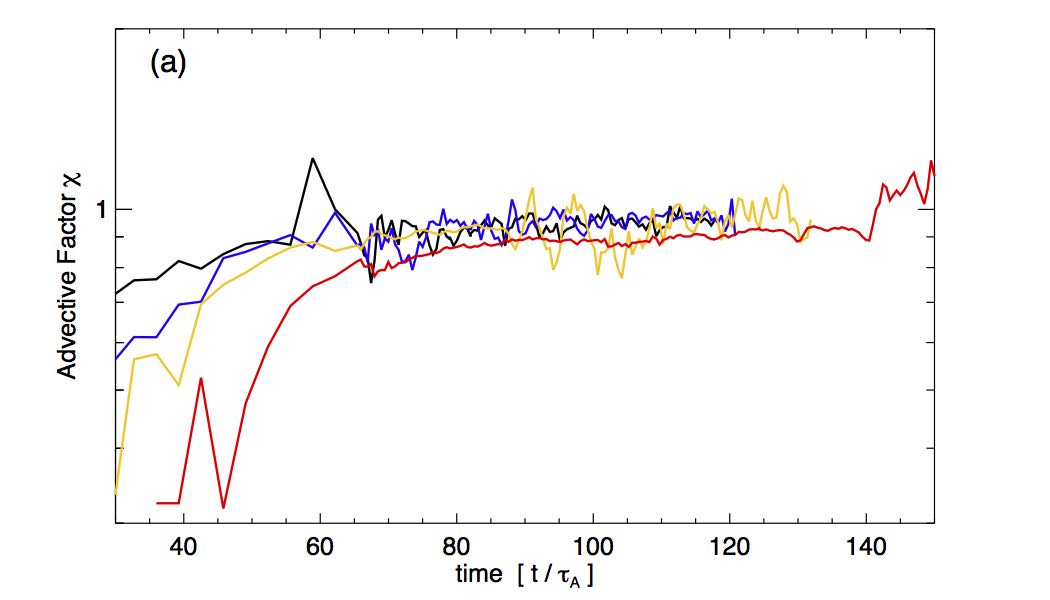
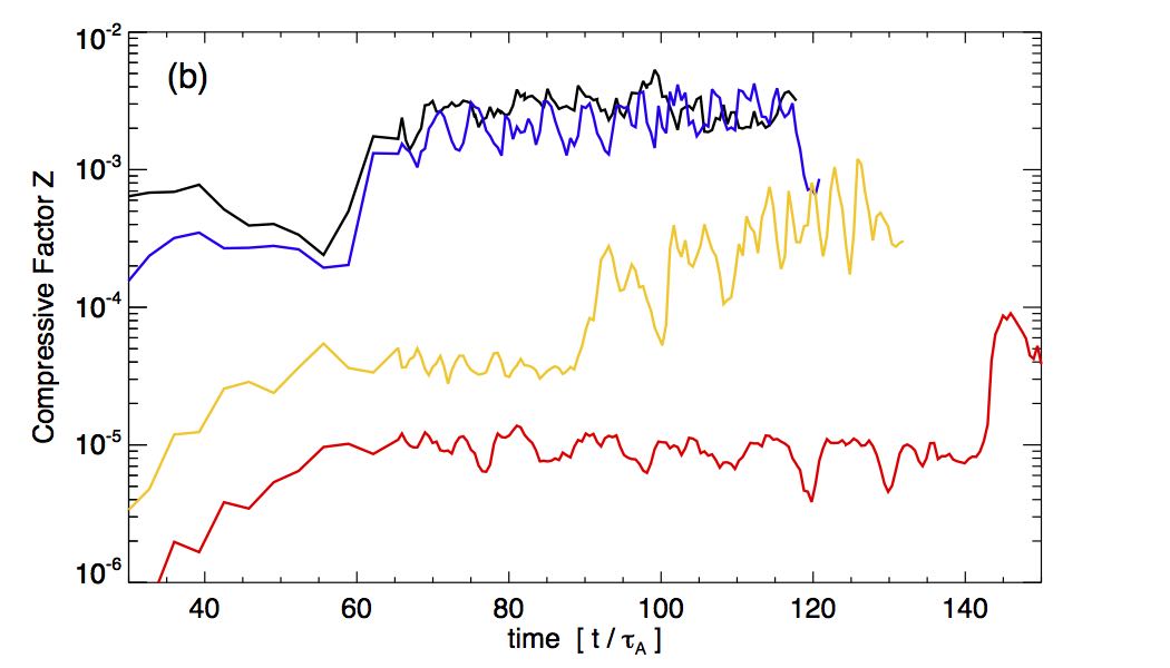
Figure 4: (a) Advective correction factor $\chi$. (b) Compressive correction factor $Z$.

In Figure 3(d) we show estimate the local Lundquist number in the vicinity of the current sheet given by,

$$S\simeq\frac{\langle\ L_{CS}\ \rangle\ \langle\ V_{Ain}\ \rangle}{\langle\ \eta\ \rangle}=\frac{4\left(\ 1+\zeta^{2}\ \right)^{1/2}}{M_{Ain}}\ \frac{\langle\ L_{CS}\ \rangle}{\delta}.$$ (12)

In all cases, since the dissipation scale $\delta$ is fixed by the gird resolution, the Lundquist estimate increases as the current sheet opens, i.e., linearly with both $\langle\ L_{CS}\ \rangle$ growth, as well as with increasing guide field strength, $|\zeta|$. The linear dependence on the current sheet length is consistent with Figure 3(b) (on the semi-log scale) prior to the jump discontinuity at nonlinear onset. Furthermore, the guide field strength dependence is evident in the approximate ordering of the curves. With the improved numerical resistivity estimate of Equation (9), the local Lundquist number beyond nonlinear onset converges to approximately $S\sim 10^{4}$.

In all simulation cases, the nonlinear onset time is ordered by the magnitude of the guide field, as expected, since the inclusion of the guide field reduces the overall magnitude of the magnetic field gradients in the vicinity of the diffusion region. This effect is also evident in Figure 5 which shows the $z=0$ transverse plane of $|J|$ with representative field lines for each current sheet simulation at $t/\tau_{A}=117.79$. It is clear that the strong guide field case, panel (d) of Figure 5, has not yet entered the nonlinear evolution, plasmoid-generation regime.

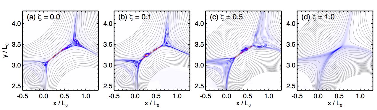
Figure 5: The current sheet development in the $z=0$ transverse planes in each of the simulations at $t=117.79\ \tau_{A}$ shows the delay of the onset of non-linear dynamics of the plasmoid instability with increasing guide field strength. Panel (a) $\zeta=0.0$; panel (b) $\zeta=0.1$; panel (c) $\zeta=0.5$; and panel (d) $\zeta=1.0$.

3.2 Qualitative Guide Field Influence on Reconnection-Generated Structure

Qualitatively, the general picture is that the guide field not only delays the dynamics by reducing the field gradients in the vicinity of the current sheet, but also increases the structure coherency in the same direction. We illustrate this in Figures 6–9 at $t=117.79\ \tau_{A}$ (consistent with Figure 5) for the zero, weak, and moderate guide field cases ($\zeta=0$, $\zeta=0.1$, and $\zeta=0.5$) which we describe below. We note, the strong $\zeta=1.0$ guide field case has not yet transitioned to non-linear evolution. Figures 6–8 each have their corresponding animations included as electronic supplements to the online version of the article.

In Figure 6, upper panel, we plot properties of the $\zeta=0$ current sheet in local, current-sheet centered coordinates: top row, intensity of the current density; middle row, the mass density ratio relative to the initial state; and bottom row, the normalized outflow velocities. The guide field direction is along $\hat{z}$ and the $\hat{e}_{1}$ direction is parallel to the current sheet (see Appendix B for details). The perspective is observing the current sheet dynamics from the top left corner of the panels of Figure 5. The main result from Paper I was that, for the $\zeta=0$ case, the magnetic reconnection occurs in different transverse planes and proceeds essentially independently from one another. Specifically, there was almost no longitudinal ($\hat{z}$-direction) coherency in the reconnection-generated density enhancements and field structure within the current sheet. This is seen in Figures 6 as the collimation of the current density, mass density, and outflow velocities along the $\hat{e}_{1}$-direction.

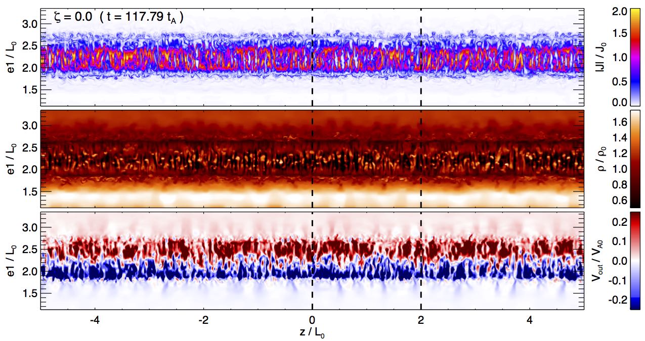
Figure 6: Zero guide field case ($\zeta=0.0$) at $t=117.79\ \tau_{A}$. Upper panel: current density magnitude $|J|/J_{0}$ (top), mass density ratio $\rho/\rho_{0}$ (middle), and outflow velocity $V_{out}/V_{A}$ (bottom).
(An animation of this figure is available)

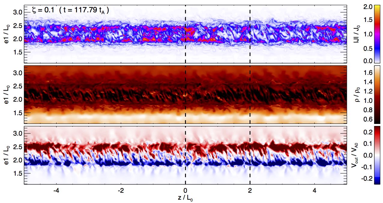
Figure 7: Weak guide field case ($\zeta=0.1$) at $t=117.79\ \tau_{A}$ in the same format as Figure 6.
(An animation of this figure is available)

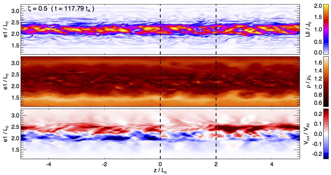
Figure 8: Moderate guid field case ($\zeta=0.5$) at $t=117.79\ \tau_{A}$ in the same format as Figure 6.
(An animation of this figure is available)

Figure 7 shows the $\zeta=0.1$ guide field case in the same format as Figures 6. This case has more coherent structure in the $z$-direction, despite being almost identical to the $\zeta=0$ case in the global reconnection properties (c.f. properties in Figure 3). We note that Lynch et al. (2016) discussed how even a relatively weak guide field in the reconnection inflow regions can generate a broader distribution of localized, stronger concentrations of guide field (and current and mass densities) during plasmoid formation in plasmoid-unstable current sheets.

Figure 8 shows the $\zeta=0.5$ guide field case in the same format as Figures 6 and 7. The moderate guide field simulation generates significantly more extended current density, mass density, and reconnection jet outflow structure along the $\hat{z}$-direction of the current sheet.

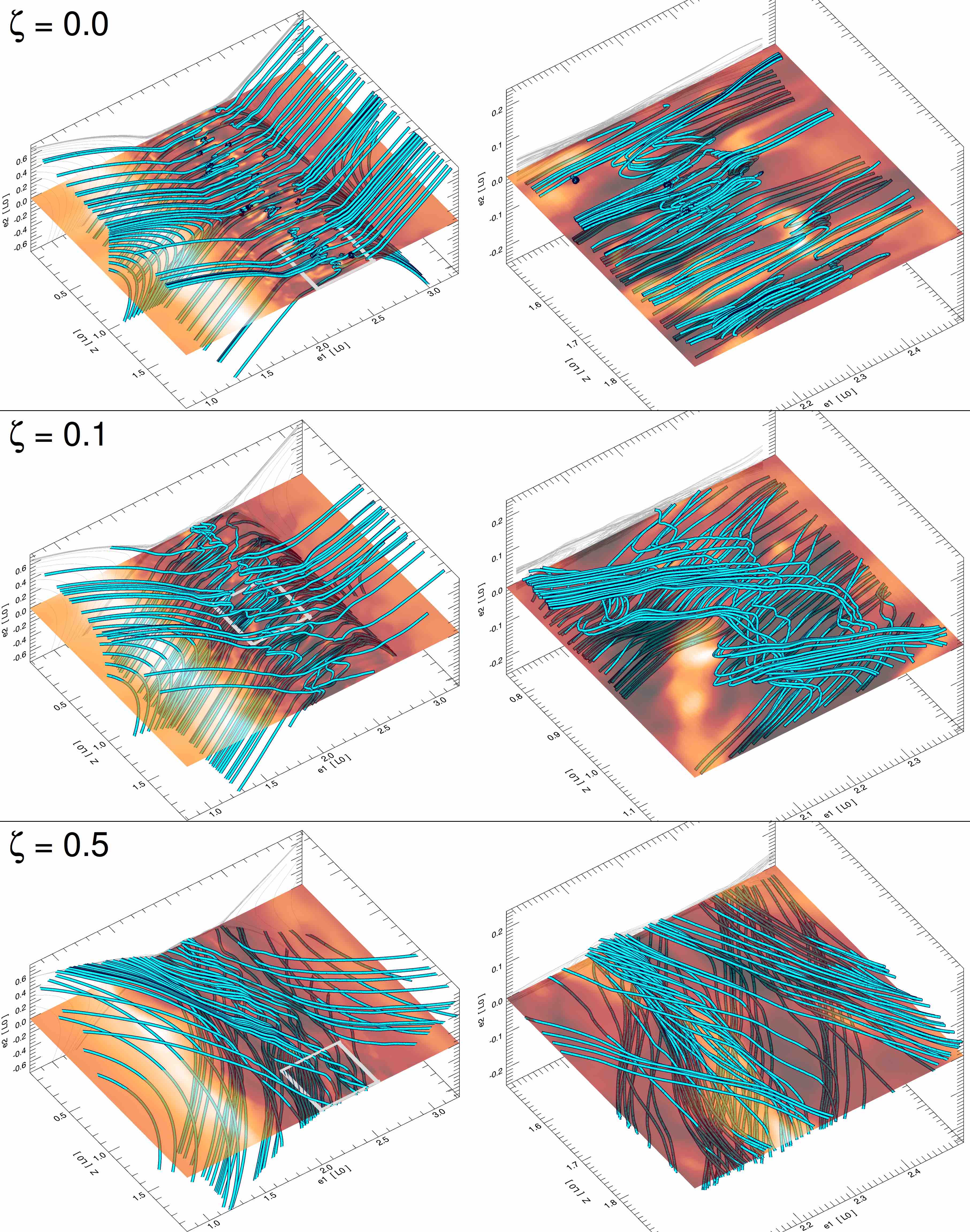
Figure 9: Three-dimensional view of representative magnetic field lines through mass density ratio $e_{2}=0$ plane for $z/L_{0}\in\left[0,2\right]$ from Figures 6–8. Top panel: $\zeta=0.0$; Middle panel: $\zeta=0.1$; Bottom panel: $\zeta=0.5$.

Figure 9 shows 3D views of representative magnetic field lines in the $z/L_{0}\in[0,2]$ subvolume centered on the current sheet. The semi-transparent $e_{2}=0$ planes in each panel shows the mass density ratio within the vertical dashed lines of Figures 6–8. Figure 9 visually confirms that the current sheet mass density enhancements are signatures of 3D magnetic islands (qualitatively similar to Daughton et al., 2011a, Figures 1a and 4) Figure 9, top panel, shows that the $\zeta=0$ twisted field lines characteristic of 3D magnetic island structures in the guide field case have an approximate longitudinal coherency of $\delta/L_{0}\sim 10^{-2}$, corresponding to approximately 2–3 grid planes—roughly the width of the plasmoid density enhancement in the transverse plane. Furthermore, the largest $\zeta=0$ structure coalescence grows to approximately $0.1L_{0}$ before ejection. Figure 9, middle panel, shows multiple, coherent twisted flux ropes on the order of $\sim 0.5L_{0}$ in length in the current sheet in the $\zeta=0.1$ case. Figure 9, bottom panel, shows that the 3D magnetic island flux rope coherency in the $\zeta=0.5$ case extends even further, reaching lengths on the order of $\sim 1-2L_{0}$ in the guide field direction.

3.3 Quantifying Reconnection-Generated Coherency Scales Due to the Guide Field

We quantify the coherency scales associated with the plasmoid density fluctuations generated during the nonlinear phase of magnetic reconnection and use these scales to analyze the Fourier power spectra. While our system is not “turbulent” per se, we will show that the statistical and spectral properties of the reconnection-generated density fluctuations in our current sheets can be understood in terms of the traditional turbulence regime classifications of energy injection and continuation range, inertial range, and dissipation scale. The coherency scales of our plasmoid formation and evolution are defined by the following transitions between these regimes:

1. the minimum structure formation coherency scale is the transition between the energy injection (structure formation) range, and the so-called energy continuation range;

2. the maximum inertial range scale is the transition between the energy continuation range and the traditional turbulent inertial range; and

3. the dissipation scale is set by the maximum numerical resolution of our MHD simulations.

In each transition, there is a marked break between spectral indices.

During the non-linear evolution phase, the AMR covers the current sheet with the highest level of grid refinement. Since there is no physical dissipation scale imposed on our simulations, we take the numerical dissipation scale as three times the maximum grid resolution, $\xi_{D}=z_{D}/L_{0}=3\ \delta/L_{0}=1.5\times 10^{-3}$.

3.3.1 Minimum Structure Formation Coherency Scale

Wavelet methods are commonly used to characterize structure coherency scales in non-steady signals (e.g., see Edmondson et al., 2013, and references therein). In this analysis, we employ the Morlet wavelet transform of the normalized mass density, $\rho(z)/\rho_{0}$, given by,

$$W_{\rho}(z,\xi)=\int\frac{\rho(z^{\prime})}{\rho_{0}}\ \psi^{*}(z^{\prime},z,\xi)\ dz^{\prime}\ ,$$ (13)

$$\psi\left(z^{\prime},z,\xi\right)=\frac{\pi^{1/4}}{|\xi|^{1/2}}{\rm exp}\left[i\omega_{0}\left(\frac{z^{\prime}-z}{\xi}\right)\right]{\rm exp}\left[-\frac{1}{2}\left(\frac{z^{\prime}-z}{\xi}\right)^{2}\right]\ ,$$ (14)

where $z^{\prime}$, $z$ are spatial coordinates in the longitudinal direction along the current sheet, $\xi$ is therefore the longitudinal spatial coherency scale, and $\omega_{0}$ is a fixed non-dimensional frequency parameter (set to $\omega_{0}=6$). The integrated power per scale (IPPS), obtained from the rectified wavelet power spectrum as

$${\rm IPPS}(\xi)=\int dz\ |\xi|^{-1}\ |W_{\rho}\left(z,\xi\right)|^{2},$$ (15)

is a modified proxy measure of the Fourier power. The rectification is necessary due to a bias in favor of large timescale features in the canonical power spectrum, which are attributed to the width of the wavelet filter in frequency space (at large timescales the function is highly compressed yielding sharper peaks of higher amplitude, whereas at small timescales the wavelet filter is broad, underestimating the high frequency peaks). The modification from the standard Fourier power spectrum is due to the wavelet cone-of-influence, which acts as a high-pass filter, attenuating the lowest frequency structures.

At each time step, in all simulation cases, we calculate the IPPS$(\xi)$ for every one-dimensional longitudinal mass density slice, $\rho(z)/\rho_{0}$, within the current sheet at that time step. The left column of Figure 10 plots the rectified wavelet IPPS$(\xi)$ spectra for each 1D-data array (green) within the current sheet at an sample time $t=109.229\ \tau_{A}$ for each $\zeta=\{0.0,0.1,0.5\}$ simulation. From all the IPPS spectra in each current sheet at each time, we calculate a distribution of global maximum IPPS values. We interpret the spatial coherency scale corresponding to the average global maximum of the set of IPPS spectra to be the minimum structure formation coherency scale $\xi_{I}$ with $\pm$1$\sigma_{I}$ uncertainty. In canonical turbulence, the structure formation/energy injection range is all coherency scales $\gtrsim\xi_{I}$.

The key point shown in the left column of Figure 10, is that with increasing guide field strength the minimum structure coherency formation scale increases from $\sim$0.15 to $\sim$0.70. The minimum coherency formation scales $\xi_{I}$ and corresponding $\pm 1\sigma_{I}$ uncertainty are tabulated for each guide field case $\zeta$ in Table 1. The shape of the spectra at smaller spatial scales (higher spatial frequencies) also shows the increasing development of a power-law character.

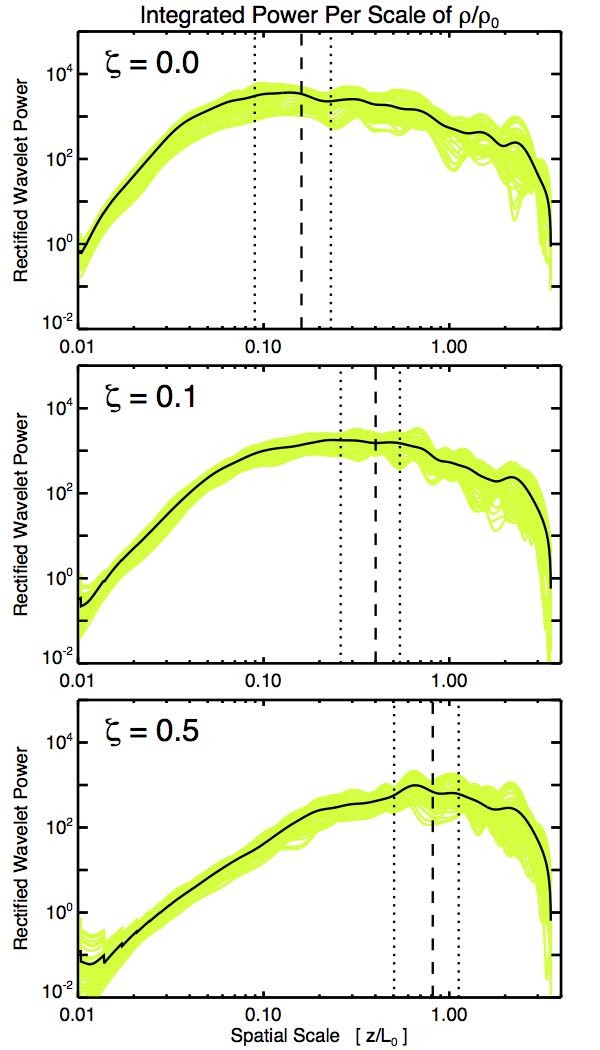
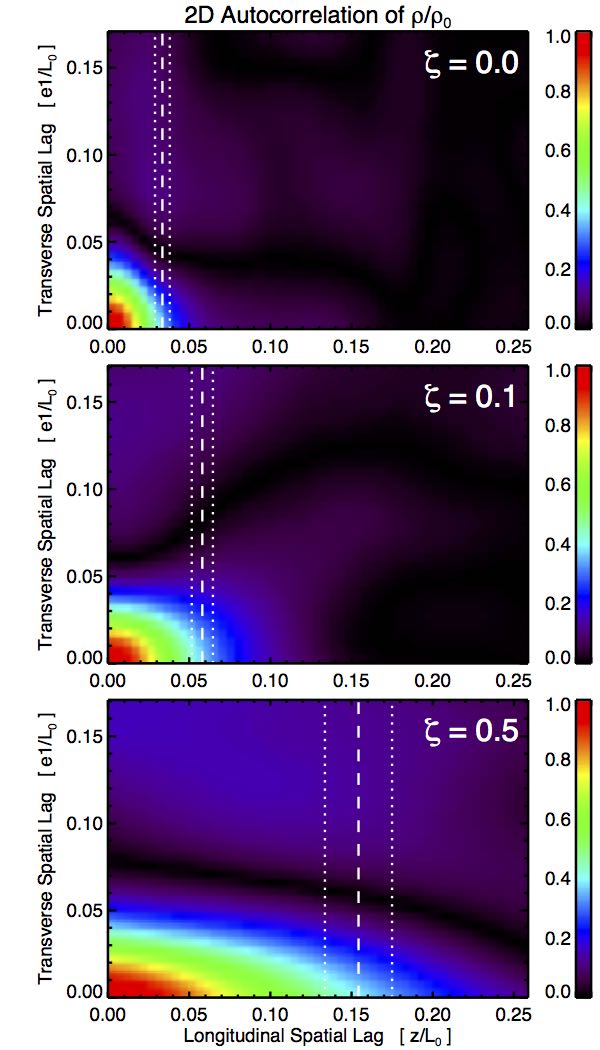
Figure 10: Left column: Rectified wavelet integrated power per scale of the density fluctuations in the current sheet for $\zeta=0.0$ (top), $\zeta=0.1$ (middle), and $\zeta=0.5$ (bottom) simulations. The minimum structure formation coherency scales are indicated with the vertical dashed lines. Right column: 2D autocorrelation functions of plasmoid density fluctuations in each of the CSs. The maximum inertial range scales are indicated with the vertical dashed lines.

3.3.2 Maximum Inertial Range Scale

Statistical autocorrelation methods are commonly used to characterize coherency scales (Zurbuchen et al., 2000). In this analysis, we calculate the discrete two-dimensional autocorrelation function of the normalized mass density $\rho(\bm{r})/\rho_{0}$ sampled in the current sheet plane where $\bm{r}$ is the position vector in the $e_{1}$-$z$ plane. The discrete 2D autocorrelation function is given by

$$A(\lambda,\mu)=\frac{\displaystyle\sum_{l=0}^{L-\lambda-1}\sum_{m=0}^{M-\mu-1}\left(\ \rho_{l,m}/\rho_{0}-<\rho/\rho_{0}>\ \right)\left(\ \rho_{l+\lambda,m+\mu}/\rho_{0}-<\rho/\rho_{0}>\ \right)}{\displaystyle\sum_{l=0}^{L-1}\sum_{m=0}^{M-1}\left(\ \rho_{l,m}/\rho_{0}-<\rho/\rho_{0}>\ \right)^{2}}\ ,$$ (16)

where $<\rho/\rho_{0}>$ is the mean density enhancement within the current sheet. The subscripts $l,m$ denote the value of the normalized density, $\rho_{l,m}/\rho_{0}$, at the grid point with label $l$ in the $z$-direction and $m$ in the $e_{1}$-direction. $\lambda$ and $\mu$ are fixed discrete spatial lag values in the $z$- and $e_{1}$-directions, respectively; in other words, $\lambda=N\Delta z$ and $\mu=M\Delta e_{1}$ are integer ($N$ and $M$) multiples of the grid cell lengths $\Delta e_{1}=\Delta z=\delta$.

At each time step, in all simulation cases, we calculate the 2D autocorrelation for the density enhancement $\rho(\bm{r})/\rho_{0}$ within the current sheet at that time step. The right column of Figure 10 illustrates the 2D autocorrelation contours of our reconnection-generated density fluctuations in the current sheets for the $\zeta=\left\{0.0,0.1,0.5\right\}$ simulations at $t=109.229\tau_{A}$. We interpret the the $1/e$-folding contour of the 2D autocorrelation to be the maximum inertial range scale, $\xi_{A}$, of the reconnection-generated plasmoid density fluctuations within the current sheet. The longitudinal spatial lag $\xi_{A}$ is shown as the vertical dashed line with $\pm 1\sigma_{A}$ uncertainty range as vertical dotted lines. The maximum inertial scales $\xi_{A}$ and corresponding uncertainty are tabulated for each guide field case $\zeta$ in Table 1.

The key point shown in the right column of Figure 10, is that with increasing guide field strength the width of the longitudinal ($z$-direction) autocorrelation function increases significantly while the transverse ($e_{1}$-direction) autocorrelation width remains approximately constant ($\sim$ 5 - 10 $\delta/L_{0}$). This result suggests that structure coherency reflects formation only in the guide field direction, as opposed to oblique formation. This effect lends support to the idea that identified oblique structures are the consequence of more complex, 3D dynamics such as the secondary instability (e.g. Dahlburg et al., 2005).

3.3.3 Density Fluctuation Fourier Power Spectra

Having defined the relevant spatial scales in the previous sections, we are now able to interpret the Fourier power spectrum in the canonical turbulence regimes of energy injection $10L_{0}\geq\xi\geq\xi_{I}$, energy continuation $\xi_{I}\geq\xi\geq\xi_{A}$, inertial range $\xi_{A}\geq\xi\geq\xi_{D}$, and dissipation. The $\xi_{I}$ scale is the minimum structure formation coherency scale identified via the wavelet IPPS spectra ($\S$ 3.3.1), the $\xi_{A}$ scale is the maximum inertial range scale identified via 2D autocorrelation ($\S$ 3.3.2), and the $\xi_{D}$ is the dissipation scale fixed at slightly larger than the grid resolution $3\ \delta$.

Figure 11 plot representative one dimensional Fourier power spectra of the density enhancement fluctuations within the current sheet for each guide field case $\zeta=\left\{0.0,0.1,0.5\right\}$ during the linear and non-linear phases, respectively, as a function of longitudinal ($z$-direction) spatial scale $\xi$. Since a relatively strong guide field suppresses non-linear onset, the weak $\zeta=0.0$ case has turned non-linear before the current sheet is identifiable in the relatively strong $\zeta=0.5$ case; hence the top row linear phase $\zeta=\left\{0.0,0.1,0.5\right\}$ guide field cases are plotted at times $t/\tau_{A}=\left\{49.08,52.35,68.46\right\}$, respectively. Figure 11 bottom row however, shows all guide field cases well-into the non-linear phases, all at the fixed time $t=109.229\ \tau_{A}$. As in previous plots, the green curves are the entire set of Fourier spectra for each 1D-data along the $z$-direction. The thick black line is the mean spectra. The dashed and dotted vertical lines indicate the minimum structure formation coherency scale ($\xi_{I}$) and maximum inertial range scale ($\xi_{A}$) with respective $1\sigma$ uncertainties.

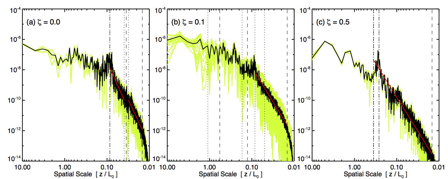
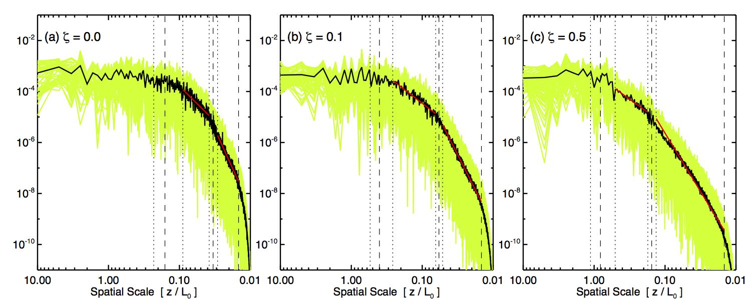
Figure 11: Density fluctuation Fourier power spectra: (a) $\zeta=0.0$; (b) $\zeta=0.1$; and (c) $\zeta=0.5$. The green are every individual FFT power spectra from 1D $\rho(z)/\rho_{0}$ along the current sheet. The solid black is the average FFT power spectra. The dashed and dotted vertical lines indicate the minimum structure formation coherency scale ($\xi_{I}$) and maximum inertial range scale ($\xi_{A}$) with respective $1\sigma$ uncertainties. The top row exhibits spectra from the linear phase at times $t/\tau_{A}=\left\{49.08,52.35,68.46\right\}$, respectively; the bottom row exhibits spectra during the non-linear phase at time $t=109.229\ \tau_{A}$.

For each simulation, we seek a power-law scaling relation for the distinct characteristic canonical turbulence ranges identified in the Fourier power spectra. The red slopes of Figure 11 illustrate these power-law fits over their respective spectral ranges for, respectively, the energy continuation range $\xi^{-\alpha\pm\sigma_{\alpha}}$ and inertial $\xi^{-\beta\pm\sigma_{\beta}}$ range for all guide field strengths. The linear phase spectra (top row) show two characteristic regions: an energy injection region dominating the majority of large spatial scales, and an inertial range beginning at typical scales of order $0.1-0.3\ z/L_{0}$. In contrast, the non-linear phase spectra (bottom row) of all cases shown exhibit three characteristic regions in their respective nonlinear phase: energy injection, energy continuation, and inertial range.

In Figure 12 we plot the two identified longitudinal coherency scales’ $\xi_{I}$ (upper data) and $\xi_{A}$ (lower data), as a function of the normalized guide field strength $\zeta$. To within the calculated $\pm 1\sigma$ uncertainties, the increase in longitudinal spatial scale increases reasonably linearly with increasing (normalized) guide field strength.

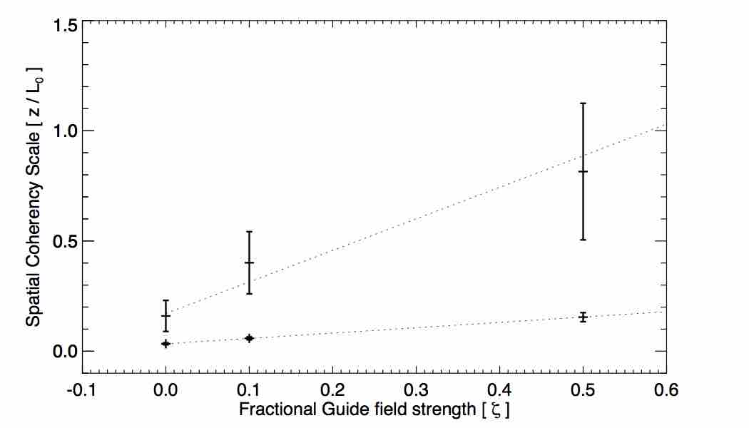
Figure 12: Longitudinal coherency scale dependence on normalized guide field strength $\zeta$. The three upper points show the minimum structure formation coherency scale $\xi_{I}$ and the three lower points show the maximum inertial range scale $\xi_{A}$.

Table 1 lists the time-averaged structure coherency scales, $\xi_{I}$, $\xi_{A}$, with their respective $\pm 1\sigma$ uncertainties, as well as the time-averaged power-law exponents, $\alpha$, $\beta$, with their respective $\pm 1\sigma$ uncertainties, obtained from all output data files (every 0.5 $\tau_{A}$) in each simulation for $109.229\leq t/\tau_{A}\leq 120$. It is clear from Figures 11 and 12, as well as Table 1, that all of our structure coherency scales increase with guide field strength, as expected. Furthermore, the energy continuation exponents are constant and independent guide field strengths to within their respective $\pm 1\sigma$ uncertainties, whereas there is a statistically significant decrease in the inertial range exponent with increasing guide field. The increased width of the inertial range with increased guide field strength, as well as the softer the power-law slope, represents the continued development of a turbulence-like distribution of density fluctuation scale sizes in the plane of the current sheet. As the characteristic “energy injection” length scale of magnetic island plasmoids increase with the guide field strength, there is more opportunity for the kinking, break up, and other nonlinear interactions to cascade this fluctuation“energy” through a broader range of scale sizes.

Guide Field	Min. Formation	Eng. Continuation Rng.	Max. Inertial	Inertial Rng.	Dissipation
Strength	Scale	Exponent	Scale	Exponent	Scale
$\zeta$	$\xi_{I}\pm\sigma_{I}$	$\alpha\pm\sigma_{\alpha}$	$\xi_{A}\pm\sigma_{A}$	$\beta\pm\sigma_{\beta}$	$\xi_{D}$
0.0	0.160 $\pm$ 0.070	2.875 $\pm$ 0.930	0.032 $\pm$ 0.004	6.161 $\pm$ 0.994	0.015
0.1	0.401 $\pm$ 0.141	2.225 $\pm$ 0.615	0.056 $\pm$ 0.006	5.541 $\pm$ 0.347	0.015
0.5	0.815 $\pm$ 0.310	2.004 $\pm$ 1.330	0.151 $\pm$ 0.020	4.582 $\pm$ 0.166	0.015

Table 1: Power-law fit exponents for each of the spatial scale ranges in the density Fourier power spectra described in Section 3.3.3 for simulations $\zeta=\{0.0,0.1,0.5\}$. The power-law exponent $\alpha$ corresponds to the continuation range, $\xi_{I}\geq z/L_{0}\geq\xi_{A}$, defined between the maximum wavelet IPPS scale ($\xi_{I}$) and the autocorrelation spatial lag ($\xi_{A}$). The power-law exponent $\beta$ corresponds to the inertial range, $\xi_{A}\geq z/L_{0}\geq\xi_{D}$, defined between $\xi_{A}$ and the dissipation scale $\xi_{D}$. See text for details.

4 Reconnection-Driven Solar Wind Outflow from Pseudostreamers

Our simulation results have the following implications for reconnection-driven solar wind outflow from pseudostreamers.

First, magnetic reconnection generates highly structured density fluctuations corresponding to 3D magnetic islands even under relatively gentle (i.e. quasi-steady state) reconnection inflow conditions. These plasmoids propagate through the current sheet and either become part of the pseudostreamer’s closed flux system or are on magnetic field lines that have interchange-reconnected and are part of the structured, intermittent reconnection outflow along the pseudostreamer external spine fan corresponding to the Separatrix-Web arc (Antiochos et al., 2011; Higginson et al., 2017b). Our results confirm the smooth interchange reconnection pseudostreamer outflow scenario of Masson et al. (2014) and show with a sufficiently resolved current sheet, the plasmoid instability during reconnection provides a potential explanation for some of the variability observed in pseudostreamer wind (Crooker et al., 2012, 2014; Owens et al., 2014).

Second, the characteristic coherency scales of our reconnection-generated density fluctuations in the plane of the current sheet are strongly a function of guide field strength. In other words, with no guide field ($\zeta=0$), the density fluctuations are essentially isotropic with a scale of $\sim$400 km whereas in the weak ($\zeta=0.1$) and moderate ($\zeta=0.5$) guide field cases they become increasingly elongated in the guide field direction with scales of $\sim$600 km and $\sim$1500 km, respectively. Given the transverse scales remain constant at $\sim$400 km, this corresponds to an increasing guide-field aligned density fluctuation axial ratio of 1.0, 1.5, and 3.8. Radio, white light, and EUV remote sensing observations show significant field-aligned and highly-collimated density structures/striations (e.g. Woo & Habbal, 2003; Druckmüller et al., 2014; Raymond et al., 2014). Interplanetary scintillation observations by Grall et al. (1997) showed relatively high axial ratios for electron density fluctuations $\delta N_{e}$ of $\gtrsim 10$ close to the sun ($\lesssim 5\ R_{\odot}$) that decreased rapidly to $\lesssim 3$ for distances $>5\ R_{\odot}$. Our idealized simulations’ density fluctuation axial ratios are consistent with the lower end of the observed ranges and we are looking forward to investigating the propagation and evolution of these signatures into a solar wind outflow (e.g. Karpen et al., 2017; Uritsky et al., 2017).

Third, the coherency of the magnetic structure of the 3D magnetic island flux ropes in the guide field direction is also directly related to the guide field strength. The representative magnetic field lines in the Figure 9 visualizations show the increasing flux rope sizes in the plane of the current sheet. Wyper et al. (2016) described the formation and evolution of 3D magnetic island flux ropes during the reconnection associated with coronal jets and essentially the same picture holds for our extended pseudostreamer arcade as well. Reconnection forms a localized region of highly twisted field in the 3D magnetic island but the field lines that make up this newly-reconnected open flux tube are relatively untwisted far from the current sheet. Therefore, the twist itself will propagate away as torsional Alfvénic waves from the reconnection site in both directions in an attempt to spread out along the field lines as much as possible (see $\S$5.2 and Figure 9 of Wyper et al. 2016). These Alfvénic fluctuations propagate both down the flux tube toward the lower boundary and along the direction of the flux tube that opens up into the solar wind. Thus, depending on the guide field strength during the interchange reconnection process, in addition to highly-structured density fluctuation outflow, one may also see periods of highly-structured magnetic field fluctuations or Alfvénic field rotations in pseudostreamer wind (e.g., see Higginson et al., 2017c).

5 Summary and Conclusions

We have extended the analysis of Paper I by analyzing a new set of 3D MHD simulations with a systematically increasing guide field component. We quantified both the longitudinal and transverse coherency scales of the mass density fluctuations generated during the nonlinear phase of plasmoid-unstable reconnection in a model solar corona and have shown that the increasing guide field strength has two main effects on our system. First, the onset of magnetic reconnection and transition to the nonlinear phase of the plasmoid instability is delayed with increasing guide field component. Second, the longitudinal coherency of the reconnection-generated 3D magnetic island flux ropes significantly increases with guide field strength.

In this set of simulations, the delay in nonlinear plasmoid-unstable onset is due to the numerical resistivity which depends on the local gradients in the magnetic fields and flows. The transition from strictly anti-parallel reconnection (no guide field) to component reconnection (a strong guide field) corresponds to a smoothing out of the total field gradient across the current sheet. This smoothing has the effect of reducing the effectiveness of the numerical diffusion. This result is well known from previous reconnection studies and we have demonstrated its applicability to systems with fully consistent, 3D current sheet formation in response to the imposed separation of the spine lines in the Syrovatskii scenario.

We have established the correspondence between the plasmoid density enhancement fluctuations in the plane of the current sheet with the 3D magnetic island flux rope structures, and hence the coherency scales of the density enhancements as a proxy for the full flux rope structures. Using standard spectral and correlation methods, we demonstrated the longitudinal structure coherency increases with guide field, whereas the transverse structure coherency remains independent of the guid field strength.

We interpret the Fourier power spectra of the plasmoid density fluctuations within the current sheet with respect to canonical turbulence, defining the corresponding energy injection range (of coherent structure formation), the energy continuation range transition, and an inertial range. We quantified how the guide field impacts the spatial scale boundaries of these ranges and the spectral slopes in each of these regions.

Finally, we have discussed the implications of our simulation results for properties of interchange-reconnection generated solar wind outflow in the vicinity of coronal pseudostreamers.

Appendix A Improved Estimate of the Numerical Resistivity

In this appendix, we derive an improved estimate of the numerical resistivity. This improved estimate is based on a simple energy density transport through the dissipative region. In other words, we balance the convective transport of the kinetic and magnetic energy densities against the Ohmic dissipation within the current sheet,

$$\oint_{A}\ \left(\ \frac{B^{2}}{8\pi}+\frac{\rho V^{2}}{2}\ \right)\bm{V}\cdot{\rm d}\bm{S}=\int_{V}\ \eta\ J^{2}\ {\rm d}V.$$ (A1)

We consider the dissipation region to be a volume with dimensions: cross-sectional thickness $\delta$ and cross-sectional length $L$, and perpendicular depth $D$. Relative to the global Cartesian coordinates used in this paper, the cross-sectional plane is spanned by the $x$-$y$ directions, and the perpendicular depth is identified with the $z$-direction. Hence, we may write equation (A1) as

$$\left(\ \frac{B^{2}}{8\pi}+\frac{\rho V^{2}}{2}\ \right)_{in}V_{in}\ L\sim\left(\ \frac{B^{2}}{8\pi}+\frac{\rho V^{2}}{2}\ \right)_{out}V_{out}\ \delta+\eta\ J^{2}\ L\delta\\$$ (A2)

For simplicity, and without loss of generality, we assume the in-states, and out-states, are equivalent on the respective right/left boundaries of the current sheet ($V_{in}^{(+)}=V_{in}^{(-)}$, $V_{out}^{(+)}=V_{out}^{(-)}$, $B_{in}^{(+)}=B_{in}^{(-)}$, and $B_{out}^{(+)}=B_{out}^{(-)}$).

We estimate $J^{2}$ through the dissipation region’s cross sectional area from Ampere’s Law (in cgs units),

$$\frac{4\pi}{c}\ \int_{A}\ \bm{J}\cdot{\rm d}\bm{S}=\oint_{C}\bm{B}\cdot{\rm d}\bm{\ell}\\$$ (A3)

Applied to the dissipation volume

$$\frac{4\pi}{c}\ J\ L\ \delta\sim 2\ B_{in}\ L+2\ B_{out}\ \delta\\$$ (A4)

Hence, we estimate $J^{2}$ in terms of $B_{in}$, $B_{out}$, and the cross sectional geometry

$$J^{2}\sim\left(\ \frac{c}{4\pi}\ \right)^{2}\left(\ \frac{2B_{in}}{\delta}\ \right)^{2}\left(\ 1+\frac{B_{out}}{B_{in}}\ \frac{\delta}{L}\ \right)^{2}\\$$ (A5)

Substituting (A5) into (A2), we estimate the numerical resistivity scales as

$$\eta\sim\frac{4\pi}{c^{2}}\ \frac{V_{in}\ \delta}{4}\left(\ 1+\frac{B_{out}}{B_{in}}\ \frac{\delta}{L}\ \right)^{-2}\left[\ \left(\ 1+\frac{V_{in}^{2}}{V_{Ain}^{2}}\ \right)-\frac{V_{out}}{V_{in}}\left(\ \frac{B_{out}^{2}}{B_{in}^{2}}+\frac{\rho_{out}}{\rho_{in}}\ \frac{V_{out}^{2}}{V_{Ain}^{2}}\ \right)\frac{\delta}{L}\ \right]\\$$ (A6)

where $V_{Ain}=B_{in}/\sqrt{4\pi\rho_{in}}$ is the (average) Alfvén speed in the in-flow region.

Hence, modulo the constant factor $4\pi/c^{2}$, we estimate the numerical resistivity as

$$\eta\sim V_{in}\ \delta\ \frac{\left(\ \chi+Z\ \right)}{4}.\\$$ (A7)

We define, to first order in $\delta/L$, the dimensionless factors for the advection of magnetic energy density $\chi$ and compressibility $Z$, respectively,

$$\chi=1-\left(\ 2\ \frac{B_{out}}{B_{in}}+\frac{V_{out}}{V_{in}}\ \frac{\mathcal{ME}_{out}}{\mathcal{ME}_{in}}\ \right)\frac{\delta}{L}\\$$ (A8)

$$Z=M_{A}^{2}\left[\ 1-\left(\ 2\ \frac{B_{out}}{B_{in}}+\frac{V_{out}}{V_{in}}\ \frac{\mathcal{KE}_{out}}{\mathcal{KE}_{in}}\ \right)\frac{\delta}{L}\ \right]\\$$ (A9)

Where $\mathcal{ME}=B^{2}/(8\pi)$ is the magnetic energy density advected with the in/out-flows, $\mathcal{KE}=\rho\ V^{2}/2$ is the kinetic energy density advected with the in/out-flows, and $M_{A}=V_{in}/V_{Ain}$ is the Alfvénic Mach number of the in-flow.

The results in Figure 3, including the current sheet aspect ratio, $\eta$, and $S$ for each of the simulation cases $\zeta=\{0,0.1,0.5,1.0\}$ are calculated using the current sheet length estimate $L_{cs}(t)$ and time-dependent, current sheet-averaged quantities $\langle V_{in}\rangle$, $\langle V_{out}\rangle$, $\langle B^{2}_{in}\rangle$, $\langle B^{2}_{out}\rangle$, and $\langle V_{Ain}\rangle$ described in the next section.

Appendix B Constructing Average Quantities in Current Sheet Coordinates

We use a slightly simpler and more automated version of the procedure outlined in the Appendices of Lynch et al. (2016) to define a current sheet-aligned coordinate transform to construct the average current sheet quantities required for the estimates of the Lundquist number $S(t)$, the numerical resistivity estimate $\eta(t)$, and to analyze the mass density fluctuations and their evolution in the plane of the current sheet in Section 3.

Using the spatial position of grid cells in the $x$-$y$ plane at $z=0$ at each simulation output time $t_{k}$, we perform a linear least-squares fit $f_{k}(x)=c_{0}+c_{1}x$, to the quantity $|J(x_{i},y_{j})|/|B(x_{i},y_{j})|\geq\Gamma$ where the parameter $\Gamma$ varies with guide field strength ($\Gamma\geq 100$ for $\zeta=0$; $\Gamma\geq 31.6$ for $\zeta=0.1$; $\Gamma\geq 100$ for $\zeta=0.5$, $\Gamma\geq 15$ for $\zeta=1.0$). We assign these spatial positions weights based on the current density magnitude $\sigma_{J}=\left(J(x_{i},y_{j})/J_{max}\right)^{4}$.

Furthermore, we define the minimum and maximum $x$-values of the spatial positions meeting a less-restrictive $\Gamma$ criteria ($\Gamma\geq 31.6$ for $\zeta=0$; $\Gamma\geq 5.0$ for $\zeta=0.1$; $\Gamma\geq 40.0$ for $\zeta=0.5$, $\Gamma\geq 2.0$ for $\zeta=1.0$) as $\left[x_{0},x_{1}\right]$ and construct their corresponding $y$-values from the current sheet fit, $\left[y_{0},y_{1}\right]=\left[f_{k}(x_{0}),f_{k}(x_{1})\right]$. The current sheet length is then simply calculated as the distance between the current sheet endpoints, $2L_{cs}=\sqrt{(x_{1}-x_{0})^{2}+(y_{1}-y_{0})^{2}}$.

We note, the above automated identification procedure worked reasonably well to fit the laminar current sheet formation stage, prior to non-linear onset (see Figure 13 panel (a)). However, in the non-linear stage, the current sheet dynamics of plasmoid formation/ejection and re-formation of the current sheet required frame-by-frame user-based visual inspection and modification of the $\left[x_{0},x_{1}\right]$ and $\left[y_{0},y_{1}\right]$ values. This simple, albeit tedious identification procedure was informed by identifying the local current sheet Y-point termini for the current sheet length, and including the largest instantaneous plasmoid for the width (see Figure 13 panel (b)).

The linear fit to the current sheet position is also used to define the current sheet coordinates $\{\ \hat{\bm{e}}_{1},\hat{\bm{e}}_{2}\ \}$, given by

$$\left[\begin{array}[]{c}\hat{\bm{e}}_{1}\\ \hat{\bm{e}}_{2}\end{array}\right]=\frac{1}{\sqrt{1+c_{1}^{2}}}\left[\begin{array}[]{cc}1&c_{1}\\ -c_{1}&1\end{array}\right]\left[\begin{array}[]{c}\hat{\bm{x}}\\ \hat{\bm{y}}\end{array}\right],$$ (B1)

where $\hat{\bm{e}}_{1}$ is parallel to the linear current sheet fit, $f_{k}$, and perpendicular $\hat{\bm{e}}_{2}$ (see Figure 13). The current sheet reconnection inflow and outflow velocity projections are now readily obtained via $V_{in}=\bm{V}\cdot\hat{\bm{e}}_{2}$ and $V_{out}=\bm{V}\cdot\hat{\bm{e}}_{1}$.

In order to construct the current sheet-averaged quantities $\langle V_{in}\rangle$, $\langle V_{out}\rangle$, $\langle B^{2}_{in}\rangle$, and $\langle B^{2}_{out}\rangle$, we define the inflow rectangular regions as centered on the $f_{k}(x)$ line extending $\pm 10\delta$ in $\hat{\bm{e}}_{2}$, and the outflow rectangular regions extending $10\delta$ in $\hat{\bm{e}}_{1}$ from each end of the current sheet (see Figure 13).

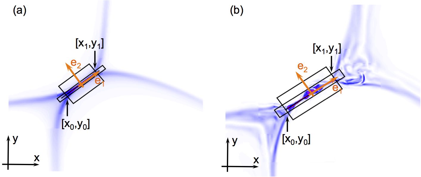
Figure 13: Current sheet identification: panel (a) automated procedure during laminar growth; panel (b) frame-by-frame user-based visual inspection procedure after non-linear onset. The current sheet coordinate direction vectors $\{\ \hat{\bm{e}}_{1},\hat{\bm{e}}_{2}\ \}$ are shown in orange. The current sheet is identified by the Y-point termini and the width of the largest plasmoid.

References

- Antiochos et al. (2002) Antiochos, S. K., Karpen, J. T., & DeVore, C. R. 2002, ApJ, 575, 578
- Antiochos et al. (2012) Antiochos, S. K., Linker, J. A., Lionello, R., et al. 2012, Space Sci. Rev., 172, 169
- Antiochos et al. (2011) Antiochos, S. K., Mikić, Z., Titov, V. S., Lionello, R., & Linker, J. A. 2011, ApJ, 731, 112
- Arge & Pizzo (2000) Arge, C. N., & Pizzo, V. J. 2000, J. Geophys. Res., 105, 10465
- Baalrud et al. (2012) Baalrud, S. D., Bhattacharjee, A., & Huang, Y.-M. 2012, Physics of Plasmas, 19, 022101
- Baker et al. (2009) Baker, D., van Driel-Gesztelyi, L., Mandrini, C. H., Démoulin, P., & Murray, M. J. 2009, ApJ, 705, 926
- Bárta et al. (2011) Bárta, M., Büchner, J., Karlický, M., & Skála, J. 2011, ApJ, 737, 24
- Biskamp (1986) Biskamp, D. 1986, Physics of Fluids, 29, 1520
- Cartwright & Moldwin (2008) Cartwright, M. L., & Moldwin, M. B. 2008, J. Geophys. Res., 113, 9105
- Cartwright & Moldwin (2010) —. 2010, J. Geophys. Res., 115, 8102
- Cassak et al. (2013) Cassak, P. A., Drake, J. F., Gosling, J. T., et al. 2013, ApJ, 775, L14
- Cassak et al. (2007) Cassak, P. A., Drake, J. F., & Shay, M. A. 2007, Physics of Plasmas, 14, 054502
- Cranmer (2012) Cranmer, S. R. 2012, Space Sci. Rev., 172, 145
- Crooker et al. (2012) Crooker, N. U., Antiochos, S. K., Zhao, X., & Neugebauer, M. 2012, J. Geophys. Res., 117, 4104
- Crooker et al. (2014) Crooker, N. U., McPherron, R. L., & Owens, M. J. 2014, J. Geophys. Res., 119, 4157
- Dahlburg et al. (2005) Dahlburg, R. B., Klimchuk, J. A., & Antiochos, S. K. 2005, ApJ, 622, 1191
- Daughton & Roytershteyn (2012) Daughton, W., & Roytershteyn, V. 2012, Space Sci. Rev., 172, 271
- Daughton et al. (2011a) Daughton, W., Roytershteyn, V., Karimabadi, H., et al. 2011a, Nature Physics, 7, 539
- Daughton et al. (2011b) Daughton, W., Roytershteyn, V., Karimabadi, H., et al. 2011b, in American Institute of Physics Conference Series, Vol. 1320, American Institute of Physics Conference Series, ed. D. Vassiliadis, S. F. Fung, X. Shao, I. A. Daglis, & J. D. Huba, 144–159
- DeVore (1991) DeVore, C. R. 1991, Journal of Computational Physics, 92, 142
- DeVore & Antiochos (2008) DeVore, C. R., & Antiochos, S. K. 2008, ApJ, 680, 740
- Drake et al. (2014) Drake, J. F., Swisdak, M., Cassak, P. A., & Phan, T. D. 2014, Geophys. Res. Lett., 41, 3710
- Drake et al. (2006) Drake, J. F., Swisdak, M., Che, H., & Shay, M. A. 2006, Nature, 443, 553
- Druckmüller et al. (2014) Druckmüller, M., Habbal, S. R., & Morgan, H. 2014, ApJ, 785, 14
- Edmondson et al. (2010a) Edmondson, J. K., Antiochos, S. K., DeVore, C. R., Lynch, B. J., & Zurbuchen, T. H. 2010a, ApJ, 714, 517
- Edmondson et al. (2010b) Edmondson, J. K., Antiochos, S. K., DeVore, C. R., & Zurbuchen, T. H. 2010b, ApJ, 718, 72
- Edmondson et al. (2009) Edmondson, J. K., Lynch, B. J., Antiochos, S. K., De Vore, C. R., & Zurbuchen, T. H. 2009, ApJ, 707, 1427
- Edmondson et al. (2013) Edmondson, J. K., Lynch, B. J., Lepri, S. T., & Zurbuchen, T. H. 2013, ApJS, 209, 35
- Feng et al. (2008) Feng, H. Q., Wu, D. J., Lin, C. C., et al. 2008, J. Geophys. Res., 113, 12105
- Fermo et al. (2010) Fermo, R. L., Drake, J. F., & Swisdak, M. 2010, Physics of Plasmas, 17, 010702
- Fujimoto (2016) Fujimoto, K. 2016, Geophys. Res. Lett., 43, 10
- Furth et al. (1963) Furth, H. P., Killeen, J., & Rosenbluth, M. N. 1963, Physics of Fluids, 6, 459
- Grall et al. (1997) Grall, R. R., Coles, W. A., Spangler, S. R., Sakurai, T., & Harmon, J. K. 1997, J. Geophys. Res., 102, 263
- Guidoni et al. (2016) Guidoni, S. E., DeVore, C. R., Karpen, J. T., & Lynch, B. J. 2016, ApJ, 820, 60
- Higginson et al. (2017a) Higginson, A. K., Antiochos, S. K., DeVore, C. R., Wyper, P. F., & Zurbuchen, T. H. 2017a, ApJ, in press, arXiv:1611.04968
- Higginson et al. (2017b) —. 2017b, ApJ, submitted, arXiv:1701.08797
- Higginson et al. (2017c) Higginson, A. K., Lynch, B. J., DeVore, C. R., et al. 2017c, ApJ, submitted
- Huang & Bhattacharjee (2010) Huang, Y.-M., & Bhattacharjee, A. 2010, Physics of Plasmas, 17, 062104
- Huang & Bhattacharjee (2012) —. 2012, Physical Review Letters, 109, 265002
- Huang & Bhattacharjee (2016) —. 2016, ApJ, 818, 20
- Janvier (2017) Janvier, M. 2017, JPlPh, 83, 535830101
- Janvier et al. (2014) Janvier, M., Démoulin, P., & Dasso, S. 2014, Sol. Phys., 289, 2633
- Karimabadi et al. (2005) Karimabadi, H., Daughton, W., & Quest, K. B. 2005, J. Geophys. Res., 110, A03213
- Karimabadi & Lazarian (2013) Karimabadi, H., & Lazarian, A. 2013, Physics of Plasmas, 20, 112102
- Karpen et al. (2017) Karpen, J. T., DeVore, C. R., Antiochos, S. K., & Pariat, E. 2017, ApJ, 834, 62
- Kepko et al. (2016) Kepko, L., Viall, N. M., Antiochos, S. K., et al. 2016, Geophys. Res. Lett., 43, 4089
- Kilpua et al. (2009) Kilpua, E. K. J., Luhmann, J. G., Gosling, J., et al. 2009, Sol. Phys., 256, 327
- Lapenta (2008) Lapenta, G. 2008, Physical Review Letters, 100, 235001
- Linton et al. (2001) Linton, M. G., Dahlburg, R. B., & Antiochos, S. K. 2001, ApJ, 553, 905
- Linton et al. (2009) Linton, M. G., DeVore, C. R., & Longcope, D. W. 2009, Earth, Planets, and Space, 61, 573
- Linton & Priest (2003) Linton, M. G., & Priest, E. R. 2003, ApJ, 595, 1259
- Loureiro et al. (2012) Loureiro, N. F., Samtaney, R., Schekochihin, A. A., & Uzdensky, D. A. 2012, Physics of Plasmas, 19, 042303
- Loureiro et al. (2007) Loureiro, N. F., Schekochihin, A. A., & Cowley, S. C. 2007, Physics of Plasmas, 14, 100703
- Lynch & Edmondson (2013) Lynch, B. J., & Edmondson, J. K. 2013, ApJ, 764, 87
- Lynch et al. (2016) Lynch, B. J., Edmondson, J. K., Kazachenko, M. D., & Guidoni, S. E. 2016, ApJ, 826, 43
- Lynch et al. (2014) Lynch, B. J., Edmondson, J. K., & Li, Y. 2014, Sol. Phys., 289, 3043
- MacNeice et al. (2000) MacNeice, P., Olson, K. M., Mobarry, C., de Fainchtein, R., & Packer, C. 2000, Computer Physics Communications, 126, 330
- Masson et al. (2013) Masson, S., Antiochos, S. K., & DeVore, C. R. 2013, ApJ, 771, 82
- Masson et al. (2012) Masson, S., Aulanier, G., Pariat, E., & Klein, K.-L. 2012, Sol. Phys., 276, 199
- Masson et al. (2014) Masson, S., McCauley, P., Golub, L., Reeves, K. K., & DeLuca, E. E. 2014, ApJ, 787, 145
- Murphy et al. (2013) Murphy, N. A., Young, A. K., Shen, C., Lin, J., & Ni, L. 2013, Physics of Plasmas, 20, 061211
- Ni et al. (2010) Ni, L., Germaschewski, K., Huang, Y.-M., et al. 2010, Physics of Plasmas, 17, 052109
- Nishida et al. (2013) Nishida, K., Nishizuka, N., & Shibata, K. 2013, ApJ, 775, L39
- Oishi et al. (2015) Oishi, J. S., Mac Low, M.-M., Collins, D. C., & Tamura, M. 2015, ApJ, 806, L12
- Owens et al. (2014) Owens, M. J., Crooker, N. U., & Lockwood, M. 2014, J. Geophys. Res., 119, 36
- Pariat et al. (2015) Pariat, E., Dalmasse, K., DeVore, C. R., Antiochos, S. K., & Karpen, J. T. 2015, A&A, 573, A130
- Pontin (2011) Pontin, D. I. 2011, Advances in Space Research, 47, 1508
- Pontin & Wyper (2015) Pontin, D. I., & Wyper, P. F. 2015, ApJ, 805, 39
- Pritchett & Coroniti (2004) Pritchett, P. L., & Coroniti, F. V. 2004, J. Geophys. Res., 109, A01220
- Pucci & Velli (2014) Pucci, F., & Velli, M. 2014, ApJ, 780, L19
- Rachmeler et al. (2014) Rachmeler, L. A., Platten, S. J., Bethge, C., Seaton, D. B., & Yeates, A. R. 2014, ApJ, 787, L3
- Rappazzo et al. (2012) Rappazzo, A. F., Matthaeus, W. H., Ruffolo, D., Servidio, S., & Velli, M. 2012, ApJ, 758, L14
- Raymond et al. (2014) Raymond, J. C., McCauley, P. I., Cranmer, S. R., & Downs, C. 2014, ApJ, 788, 152
- Riley & Luhmann (2012) Riley, P., & Luhmann, J. G. 2012, Sol. Phys., 277, 355
- Sheeley et al. (1999) Sheeley, N. R., Walters, J. H., Wang, Y.-M., & Howard, R. A. 1999, J. Geophys. Res., 104, 24739
- Shen et al. (2011) Shen, C., Lin, J., & Murphy, N. A. 2011, ApJ, 737, 14
- Shen et al. (2013) Shen, C., Lin, J., Murphy, N. A., & Raymond, J. C. 2013, Physics of Plasmas, 20, 072114
- Shepherd & Cassak (2012) Shepherd, L. S., & Cassak, P. A. 2012, J. Geophys. Res., 117, A10101
- Shibata & Tanuma (2001) Shibata, K., & Tanuma, S. 2001, Earth, Planets, and Space, 53, 473
- Shimizu et al. (2009) Shimizu, T., Kondo, K., Ugai, M., & Shibata, K. 2009, ApJ, 707, 420
- Syrovatskii (1978a) Syrovatskii, S. I. 1978a, Ap&SS, 56, 3
- Syrovatskii (1978b) —. 1978b, Sol. Phys., 58, 89
- Syrovatskii (1981) —. 1981, ARA&A, 19, 163
- Tenerani et al. (2016) Tenerani, A., Velli, M., Pucci, F., Landi, S., & Rappazzo, A. F. 2016, Journal of Plasma Physics, 82, 535820501
- Titov et al. (2012) Titov, V. S., Mikic, Z., Török, T., Linker, J. A., & Panasenco, O. 2012, ApJ, 759, 70
- Uritsky et al. (2017) Uritsky, V. M., Roberts, M. A., DeVore, C. R., & Karpen, J. T. 2017, ApJ, 837, 123
- Uzdensky et al. (2010) Uzdensky, D. A., Loureiro, N. F., & Schekochihin, A. A. 2010, Physical Review Letters, 105, 235002
- van Driel-Gesztelyi et al. (2012) van Driel-Gesztelyi, L., Culhane, J. L., Baker, D., et al. 2012, Sol. Phys., 281, 237
- Viall & Vourlidas (2015) Viall, N. M., & Vourlidas, A. 2015, ApJ, 807, 176
- Wang et al. (2015) Wang, S., Yokoyama, T., & Isobe, H. 2015, ApJ, 811, 31
- Wang et al. (2012) Wang, Y.-M., Grappin, R., Robbrecht, E., & Sheeley, Jr., N. R. 2012, ApJ, 749, 182
- Wang et al. (2000) Wang, Y.-M., Sheeley, N. R., Socker, D. G., Howard, R. A., & Rich, N. B. 2000, J. Geophys. Res., 105, 25133
- Wang et al. (2007) Wang, Y.-M., Sheeley, Jr., N. R., & Rich, N. B. 2007, ApJ, 658, 1340
- Woo & Habbal (2003) Woo, R., & Habbal, S. R. 2003, in American Institute of Physics Conference Series, Vol. 679, Solar Wind Ten, ed. M. Velli, R. Bruno, F. Malara, & B. Bucci, 55–58
- Wyper et al. (2016) Wyper, P. F., DeVore, C. R., Karpen, J. T., & Lynch, B. J. 2016, ApJ, 827, 4
- Wyper & Pontin (2014a) Wyper, P. F., & Pontin, D. I. 2014a, Physics of Plasmas, 21, 102102
- Wyper & Pontin (2014b) —. 2014b, Physics of Plasmas, 21, 082114
- Yu et al. (2014) Yu, W., Farrugia, C. J., Lugaz, N., et al. 2014, J. Geophys. Res., 119, 689
- Zurbuchen et al. (2002) Zurbuchen, T. H., Fisk, L. A., Gloeckler, G., & von Steiger, R. 2002, Geophys. Res. Lett., 29, 1352
- Zurbuchen et al. (2000) Zurbuchen, T. H., Hefti, S., Fisk, L. A., Gloeckler, G., & Schwadron, N. A. 2000, J. Geophys. Res., 105, 18327
- Zweibel & Yamada (2009) Zweibel, E. G., & Yamada, M. 2009, ARA&A, 47, 291