Theoretical investigation of two-particle two-hole effect
on spin-isospin excitations through charge-exchange reactions

Abstract

Background: Coherent one-particle one-hole (1p1h) excitations have given us effective insights into general nuclear excitations. However, the two-particle two-hole (2p2h) excitation beyond 1p1h is now recognized as critical for the proper description of experimental data of various nuclear responses.
Purpose: The spin-flip charge-exchange reactions ${}^{48}{\rm Ca}(p,n)^{48}{\rm Sc}$ are investigated to clarify the role of the 2p2h effect on their cross sections. The Fermi transition of ${}^{48}{\rm Ca}$ via the $(p,n)$ reaction is also investigated in order to demonstrate our framework.
Methods: The transition density is calculated microscopically with the second Tamm-Dancoff approximation, and the distorted-wave Born approximation is employed to describe the reaction process. A phenomenological one-range Gaussian interaction is used to prepare the form factor.
Results: For the Fermi transition, our approach describes the experimental behavior of the cross section better than the Lane model, which is the conventional method. For spin-flip excitations including the GT transition, the 2p2h effect decreases the magnitude of the cross section and does not change the shape of the angular distribution. The $\Delta l=2$ transition of the present reaction is found to play a negligible role.
Conclusions: The 2p2h effect will not change the angular-distributed cross section of spin-flip responses. This is because the transition density of the Gamow-Teller response, the leading contribution to the cross section, is not significantly varied by the 2p2h effect.

I Introduction

Several theories based on the picture of particle-hole excitations have successfully described the nuclear spin-isospin response. Not only the lowest-order one-particle one-hole (1p1h) excitation but also many-particle many-hole excitations have been observed to play a significant role. For neutrino-nucleus quasielastic scattering, the inclusion of the two-particle two-hole (2p2h) configuration enhances the cross section to the point where a theoretical calculation is consistent with the experimental data Martini et al. (2009). For a nuclear spin-isospin response, the 2p2h-configuration mixing partly explains the Gamow-Teller (GT) quenching problem, which is known not to follow the Ikeda sum rule Ikeda (1964); Fujita and Ikeda (1965); Gaarde (1983) and is one of the long-standing problems in nuclear physics. Other reasons for this quenching are the existence of the $\Delta$-$h$ excitation and the coupling of the GT-$1^{+}$ state to the spin-quadrupole (SQ) $1^{+}$ state mediated by the tensor force Bai et al. (2009). For a more detailed review, see Ref. Ichimura et al. (2006).

Recently the effect of 2p2h mixing on the GT-transition strength $B({\rm GT})$ employing the fully self-consistent second Tamm-Dancoff approximation (STDA) was investigated Minato (2016). The calculated $B({\rm GT})$ distribution of ${}^{48}{\rm Ca}$ was compared with its experimentally measured value Yako et al. (2009), which was derived through an analysis of the charge-exchange reaction ${}^{48}{\rm Ca}(p,n)^{48}{\rm Sc}$ by means of the distorted-wave impulse approximation (DWIA). It was shown that the STDA (where the 2p2h model space was confined to seven single-particle levels) described the experimental data better than the 1p1h Tamm-Dancoff approximation (TDA). It was also confirmed that the broadening of the $B({\rm GT})$ distribution by the 2p2h effect was essential to account for the observed experimental behavior, as preceding works have shown using different models Drożdż et al. (1986); Niu et al. (2014).

Charge exchange reactions such as $(p,n)$ and $(^{3}{\rm He},t)$ excite target nuclei through the one-body operator which populates 1p1h states in target nuclei. Therefore, the 2p2h configuration is not directly involved in the above reactions. However, it would have an indirect influence on the cross sections through the transition from 1p1h states to 2p2h states. Even though the importance of the 2p2h configuration in $B({\rm GT})$ has been pointed out by many authors Drożdż et al. (1986); Wakasa et al. (2012); Ichimura et al. (2006); Wambach (1988), a microscopic understanding of how such a higher-order configuration is involved in the charge-exchange cross section is not so transparent. In the present paper we therefore investigate the effect of the 2p2h configuration on the angular-distributed cross section, which is directly comparable with experimental data. In order to calculate the cross section of spin-flip transitions, we work with the distorted-wave Born approximation (DWBA) with the microscopic transition density obtained by the STDA.

The $\Delta l=2$ transition also generates $1^{+}$ resonance states at excitation energies equal to that of GT-$1^{+}$ states. When the experimental $B({\rm GT})$ of ${}^{48}{\rm Ca}$ was evaluated Yako et al. (2009), it was assumed that the zero-degree charge-exchange cross section is proportional to $B({\rm GT})$ and the $\Delta l=2$ transition plays a negligible role. The assumption, however, was confirmed only for the ${}^{13}{\rm C}(p,n)^{13}{\rm N}$ reaction Taddeucci et al. (1987). Therefore we investigate whether the assumption is valid also for the present system, ${}^{48}{\rm Ca}(p,n)^{48}{\rm Sc}$.

In this article both the spin-flip and non-spin-flip transitions are surveyed. Note that, in the Fermi transition, the nucleus populates the isobaric analogue state (IAS), which has the same isospin $T_{A}$ as that of the ground state of the parent nucleus. It does not couple to other 1p1h states having $T_{A}\pm 1$; i.e., the 2p2h effect is expected to be small for the Fermi transition as seen in outgoing neutron spectra of $(p,n)$ reactions (see, for example, Ref. Anderson et al. (1985)). Therefore we investigate the Fermi transition just to demonstrate our theoretical framework.

This paper is organized as follows. Section II is dedicated to the formulation of the structure and reaction models as well as the form factor. In Sec. III, results on the non-spin-flip (Fermi-type) transition are shown. The 2p2h effect on the cross section of the spin-flip transition is also discussed. A summary is given in Sec. IV.

II Theoretical framework

Convolution of the DWBA and the random phase approximation (which includes a correlation in ground states in addition to the TDA) is widely used to analyze experimental data at intermediate energies, as in the measurements of charge-exchange cross sections at zero degree Taddeucci et al. (1987); Love et al. (1987); Fujita et al. (2015) accompanied by the multipole decomposition technique Ichimura et al. (2006). Here we use DWBA+TDA/STDA based on the Skyrme energy density functional Vautherin and Brink (1972) in order to discuss the effect of the 2p2h configuration on charge-exchange cross sections. Because the ground state correlation is expected to be small for the Fermi- and GT-type charge-exchange reactions Nishizaki et al. (1988); Dinh Dang et al. (1997), the use of the TDA will not affect our results. We briefly describe the STDA as well as the TDA in Sec. II.1 and illustrate the formulations of the form factor and the DWBA in Secs. II.2 and II.3, respectively.

II.1 Structure model

We consider the transition $A\rightarrow B$ induced by the charge-exchange reaction $A(p,n)B$. To describe the GT and $\Delta l=2$ transitions as well as other $1^{+}$ multipole spin-flip transitions relevant to the reaction studied, we adopt the STDA as explained in Ref. Minato (2016). In the STDA the many-body wave function $\ket{B_{\alpha}}$, which is a resonance state of $B$ with respect to the $A$’s ground state $\ket{A}$, is written as

$$\ket{B_{\alpha}} =\left[\sum_{mi}X_{mi}a_{m}^{\dagger}a_{i}+\sum_{mnij}\mathcal{X}_{mnij}a_{m}^{\dagger}a_{n}^{\dagger}a_{i}a_{j}\right]\ket{A}$$

$$\equiv\sum_{mi}X_{mi}\ket{m(i)^{-1}}+\sum_{mnij}\mathcal{X}_{mnij}\ket{mn(ij)^{-1}},$$ (1)

where $a_{\nu}^{\dagger}$ ($a_{\nu}$) is the creation (annihilation) operator in the single-particle state $\nu$, and $\nu=m,n,p,q$ ($\nu=i,j,k,l$) for the particle (hole) states. We introduce the index $\alpha$ to express the non-spin-flip transition ($\alpha=s0$), the spin-flip transition ($\alpha=s1$), and the $\Delta l=2$ transition ($\alpha=l2$). We work with the Skyrme-Hartree-Fock model to obtain $\ket{A}$. The coefficients $X_{mi}$ and $\mathcal{X}_{mnij}$ are determined by solving the so-called STDA equation Yannouleas (1987),

$$\left(\begin{array}[]{cc}A&\mathcal{A}_{12}\\ \mathcal{A}_{21}&\mathcal{A}_{22}\\ \end{array}\right)\left(\begin{array}[]{c}X\\ \mathcal{X}\\ \end{array}\right)=\varepsilon\left(\begin{array}[]{c}X\\ \mathcal{X}\\ \end{array}\right).$$ (8)

Here the matrix elements in Eq. (8) are given by Ref. Yannouleas (1987) and $\varepsilon$ is the phonon energy.

A value of $\mathcal{X}_{mnij}=0$ corresponds to the standard TDA, which does not include 2p2h-configuration mixing. In the TDA, $\Ket{B_{\alpha}}$ is given by

$$\Ket{B_{\alpha}}=\sum_{mi}X_{mi}a_{m}^{\dagger}a_{i}\ket{A}.$$ (9)

The coefficients $X_{mi}$ are obtained from the so-called TDA equation; see Refs. Rowe (1970); Ring and Schuck (1980). Since the 2p2h effect on the IAS originating from the Fermi transition is known to be negligible (see Sec. I), we describe $\Ket{B_{s0}}$ by Eq. (9).

The transition density, which is employed to calculate the form factor shown later, is given by

$$g_{\alpha}(r_{i_{t}}) =\frac{1}{\hat{j}_{B}}\sum_{mi}X_{mi}R_{m}(r_{i_{t}})R_{i}(r_{i_{t}})\left\langle j_{m}l_{m}\left|\left|\mathcal{G}_{\alpha}\right|\right|j_{i}l_{i}\right\rangle,$$ (10)

where $R_{m}$ $(R_{i})$ is the radial part of the single-particle wave-function and $j_{m}=l_{m}\pm 1/2$ ($j_{i}=l_{i}\pm 1/2$) with the magnitude of the orbital angular momentum $l_{m}$ ($l_{i}$) of state $m$ $(i)$. The coordinate of the $i_{t}$ th nucleon in the target is $\bm{r}_{i_{t}}$ and $j_{B}$ is the magnitude of the spin of $B$. We use the abbreviation $\hat{j}_{B}=\sqrt{2j_{B}+1}$. The transition operator for the non-spin-flip transition is

$$\mathcal{G}_{s0}=\bm{\tau}Y_{l=0,0}(\hat{\bm{r}}_{i_{t}}),$$ (11)

and those of the spin-flip and $\Delta l=2$ transitions are, respectively,

$$\mathcal{G}_{s1} =\bm{\tau}Y_{l=0,0}(\hat{\bm{r}}_{i_{t}})\bm{\sigma},$$ (12)

$$\mathcal{G}_{l2} =\bm{\tau}\left[Y_{l=2}(\hat{\bm{r}}_{i_{t}})\otimes\bm{\sigma}\right]_{1M},$$ (13)

where $\bm{\sigma}$ ($\bm{\tau}$) is the Pauli spin (isospin) operator. Here $l$ corresponds to the orbital angular momentum transfer of the relative motion [see Eq. (20)], and $M=0,\pm 1$.

II.2 Form factor

The form factor is expressed by

$$\mathcal{F}_{\alpha}(\bm{R})=\Braket{nB\left missing}{v_{\alpha}}{pA},$$ (14)

where $\bm{R}$ is the relative coordinate of the $p$-$A$ and $n$-$B$ system. The ket (bra) vector represents the product of the spin-wave function of the projectile (ejectile) and the many-body wave function of $A$ ($B$). The transitions of non-spin-flip (the spin transfer $\Delta s=0$), spin-flip ($\Delta s=1$), and $\Delta l=2$ components are respectively caused by the interactions,

$$v_{s0} =\sum_{i_{p}i_{t}}V_{s0}(\rho)\bm{\tau}_{i_{p}}\cdot\bm{\tau}_{i_{t}},$$ (15)

$$v_{s1} =\sum_{i_{p}i_{t}}V_{s1}(\rho)\left(\bm{\sigma}_{i_{p}}\cdot\bm{\sigma}_{i_{t}}\right)\left(\bm{\tau}_{i_{p}}\cdot\bm{\tau}_{i_{t}}\right),$$ (16)

$$v_{l2} =\sum_{i_{p}i_{t}}V_{l2}(\rho)\left([\bm{\sigma}_{i_{p}}Y_{2}]_{1}\cdot[\bm{\sigma}_{i_{t}}Y_{2}]_{1}\right)\left(\bm{\tau}_{i_{p}}\cdot\bm{\tau}_{i_{t}}\right),$$ (17)

where $\rho=\left|r_{i_{p}}-r_{i_{t}}\right|$ and the sums over $i_{p}$ ($i_{t}$) represent the nucleon number of the projectile (target nucleus) running up to its mass number.

We assume that the radial parts $V_{s0}$, $V_{s1}$, and $V_{l2}$ are the one-range Gaussian functions given by

$$V_{s0}(\rho)=\bar{V}_{0}e^{-\left(\frac{\rho}{\rho_{0}}\right)^{2}},\quad V_{s1}(\rho)=V_{l2}(\rho)=\bar{V}_{1}e^{-\left(\frac{\rho}{\rho_{1}}\right)^{2}},$$ (18)

the parameters of which are determined phenomenologically. Since the present work focuses on the investigation of the 2p2h effect, we use this phenomenological interaction rather than a microscopic one.

Following the formalism of Refs. Petrovich and Stanley (1977); Cook et al. (1984), the form factor is obtained through the partial-wave expansion. The radial part of $\mathcal{F}_{\alpha}$ is calculated as

$$F_{lsj}^{\alpha}(R)=\frac{i^{l}}{\pi^{2}}\hat{j}\int\tilde{V}_{\alpha}(K)\tilde{g}_{\alpha}(K)j_{l}(KR)K^{2}dK,$$ (19)

where $s$ and $j$ are the transferred angular momenta defined by

$$\bm{j}=\bm{j}_{B}-\bm{j}_{A},\quad\bm{s}=\bm{j}_{p}-\bm{j}_{n},\quad\bm{l}=\bm{j}-\bm{s},$$ (20)

with the spin $\bm{j}_{x}$ of the particle $x$ $(=p,n,A,~{}{\rm and}~{}B)$. The interaction and transition density in momentum space, regarding $K$ associated with $R$, are respectively defined by

$$\tilde{V}_{\alpha}(K) =4\pi\int d\rho\rho^{2}\frac{\sin(K\rho)}{K\rho}V_{\alpha}(\rho),$$ (21)

$$\tilde{g}_{\alpha}(K) =4\pi\int dr_{i_{t}}\,r_{i_{t}}^{2}j_{l}(Kr_{i_{t}})g_{\alpha}(r_{i_{t}}),$$ (22)

with the spherical Bessel function $j_{l}$ ($l=0$ for the non-spin-flip and spin-flip transitions, and $l=2$ for the $\Delta l=2$ case).

Expanding the spherical Bessel function of Eq. (22) in terms of $K$, we obtain the integrands proportional to $g_{\alpha},r_{i_{t}}^{2}g_{\alpha}$, and so on. The lowest-order terms for $\alpha=s1$ and $l2$ correspond to the GT- and SQ-$1^{+}$ transitions, respectively. Incidentally, the first order for $\alpha=s1$ is the spin-monopole transition, which is difficult to distinguish from the GT transition experimentally Yako et al. (2009). Higher-order contributions can be safely ignored, as they are negligibly small in excitation energies studied in this work.

II.3 Reaction model

The following expression is based on the formalism in Ref. Cook et al. (1984) but now generalized to include the spin-orbit interaction regarding the coupling between the projectile’s (ejectile’s) spin and the $p$-$A$ ($n$-$B$) orbital angular momentum in the initial (final) channel. The transition matrix with the DWBA under the partial-wave expansion is given by

$$T^{\rm(DWBA)}_{\alpha;m_{p}m_{n}m_{A}m_{B}} =\frac{4\pi}{K_{p}K_{n}}(-)^{j_{n}+m_{n}}\hat{j}_{n}$$

$$\times\sum_{jm_{j}}\left(j_{A}m_{A}jm_{j}|j_{B}m_{B}\right)\mathcal{S}_{\alpha;jm_{j}}^{m_{p}m_{n}},$$ (23)

where $m_{j}$ and $m_{x}$ respectively correspond to the $z$-projections of $\bm{j}$ and $\bm{j}_{x}$. The magnitude of the wave number of the projectile (ejectile) is expressed by $K_{p}$ ($K_{n}$). The function $\mathcal{S}_{\alpha;jm_{j}}^{m_{p}m_{n}}$ is defined by

$$\mathcal{S}_{\alpha;jm_{j}}^{m_{p}m_{n}} =\left(4\pi\right)^{-\frac{1}{2}}\sum_{\begin{subarray}{c}J_{i}J_{f}\\ L_{i}L_{f}\\ ls\end{subarray}}i^{L_{i}-L_{f}-l}\hat{s}\hat{J}_{i}\hat{J}_{f}\hat{L}_{i}^{2}\hat{L}_{f}^{2}I_{J_{i}J_{f}L_{i}L_{f}}^{\alpha;lsj}$$

$$\times\left(L_{i}0L_{f}0|l0\right)\begin{Bmatrix}L_{f}&L_{i}&l\\ j_{n}&j_{p}&s\\ J_{f}&J_{i}&j\end{Bmatrix}f_{jj_{p}j_{n}L_{i}L_{f}}^{m_{j}m_{p}m_{n}}\left(\cos\theta\right),$$ (24)

where $L_{i}$ ($L_{f}$) is the magnitude of the orbital angular momentum regarding the relative $p$-$A$ ($n$-$B$) motion, and its coupled spin with $j_{p}$ ($j_{n}$) is expressed by $J_{i}$ ($J_{f}$). The conservation of the total angular momentum is given by

$$\left[\left[\bm{j}_{p}\otimes\bm{L}_{i}\right]_{\bm{J}_{i}}\otimes\bm{j}_{A}\right]=\left[\left[\bm{j}_{n}\otimes\bm{L}_{f}\right]_{\bm{J}_{f}}\otimes\bm{j}_{B}\right].$$ (25)

The overlap integral $I_{J_{i}J_{f}L_{i}L_{f}}^{\alpha;lsj}$ and the function $f_{jj_{p}j_{n}L_{i}L_{f}}^{m_{j}m_{p}m_{n}}$ are respectively defined as

$$I_{J_{i}J_{f}L_{i}L_{f}}^{\alpha;lsj} =\int dR\tilde{\xi}_{n;J_{f}L_{f}}(K_{f},R)F_{lsj}^{\alpha}(R)\tilde{\xi}_{p;J_{i}L_{i}}(K_{i},R),$$ (26)

$$f_{jj_{p}j_{n}L_{i}L_{f}}^{m_{j}m_{p}m_{n}}\left(\cos\theta\right)$$

$$\quad=\left(J_{i}m_{p}J_{f},m_{j}-m_{p}|jm_{j}\right)\left(j_{p}m_{p}L_{i}0|J_{i}m_{p}\right)$$

$$\quad\times\left(j_{n},-m_{n}L_{f},m_{j}-m_{p}+m_{n}|J_{f},m_{j}-m_{p}\right)$$

$$\quad\times\left[\frac{(L_{f}-\left|m_{j}-m_{p}+m_{n}\right|)!}{(L_{f}+\left|m_{j}-m_{p}+m_{n}\right|)!}\right]^{\frac{1}{2}}P_{L_{f},m_{j}-m_{p}+m_{n}}\left(\cos\theta\right),$$ (27)

with the Legendre function $P_{L_{f},m_{j}-m_{p}+m_{n}}$ as a function of the emitting angle $\theta$.

The partial wave $\tilde{\xi}_{\gamma;JL}~{}=~{}P_{\rm NL}^{(\gamma)}\xi_{\gamma;JL}$ ($\gamma=p~{}{\rm or}~{}n$) is given as the solution of the Schrödinger equation,

$$\left[\frac{d^{2}}{dR^{2}}+K_{\gamma}-\frac{L(L+1)}{R^{2}}-\frac{2\mu_{\gamma}}{\hbar^{2}}U_{\gamma}(R)\right]\xi_{\gamma;JL}(K_{\gamma},R)=0,$$ (28)

where the reduced mass is represented by $\mu_{\gamma}$ and the distorting potential $U_{\gamma}$ involves the central, spin-orbit, and Coulomb terms. Here, in order to take into account the nonlocality of the nucleon optical potential, we multiply the distorted wave $\xi_{\gamma;JL}$ by the so-called Perey factor $P_{\rm NL}^{(\gamma)}$ Perey and Buck (1962),

$$P_{\rm NL}^{(\gamma)}(R) =\left[1-\frac{\mu_{p}\beta^{2}}{2\hbar^{2}}U_{\gamma}^{\rm(N)}(R)\right]^{-\frac{1}{2}},$$ (29)

with the nonlocal parameter $\beta$ and the nuclear part $U_{\gamma}^{\rm(N)}$ of the distorting potential.

The cross section is calculated as

$$\frac{d\sigma_{\alpha}}{d\Omega} =\frac{\mu_{p}\mu_{n}}{\left(2\pi\hbar^{2}\right)^{2}}\frac{K_{n}}{K_{p}}\frac{1}{\left(\hat{j}_{p}\hat{j}_{A}\right)^{2}}\sum_{\begin{subarray}{c}m_{p}m_{n}\\ m_{A}m_{B}\end{subarray}}\left|T^{\rm(DWBA)}_{\alpha;m_{p}m_{n}m_{A}m_{B}}\right|^{2}$$

$$=\frac{1}{E_{p}E_{n}}\frac{K_{n}}{K_{p}}\left(\frac{\hat{j}_{n}\hat{j}_{B}}{\hat{j}_{p}\hat{j}_{A}}\right)^{2}\sum_{jm_{j}}\frac{1}{\hat{j}^{2}}\sum_{m_{p}m_{n}}\left|\mathcal{S}_{\alpha;jm_{j}}^{m_{p}m_{n}}\right|^{2},$$ (30)

with $E_{\gamma}=\left(\hbar K_{\gamma}\right)^{2}/(2\mu_{\gamma})$.

III Results and discussion

III.1 Model setting

The ground state wave function of ${}^{48}{\rm Ca}$ is calculated by the Skyrme-Hartree-Fock approach Vautherin and Brink (1972) with the SGII effective interaction Van Giai and Sagawa (1981). To obtain the non-spin-flip $0^{+}$ and spin-flip $1^{+}$ excited states, we solve the STDA and TDA equations with the same force in a self-consistent manner, and the transition density given by Eq. (10) is calculated for each state. The model space of the STDA and TDA calculations consists of single-particle orbits up to $100$ MeV for the 1p1h configuration and $1d_{5/2},1d_{3/2},2s_{1/2},1f_{7/2},2p_{3/2},2p_{1/2}$, and $1f_{5/2}$ orbits for the 2p2h configuration as performed in Ref. Minato (2016). The neutron and proton orbits are assumed to be fully occupied up to $1f_{7/2}$ and $2s_{1/2}$, respectively.

To calculate the form factor, we adjust the strengths $\bar{V}_{0}$ and $\bar{V}_{1}$, while keeping the range parameter fixed at $\rho_{0}=\rho_{1}=1.484$ fm Ohmura et al. (1970). For the non-spin-flip transition, we let $\bar{V}_{0}=-1762.4$ MeV in order to fit the calculated cross section to the measured data at forward angle. For the spin-flip transitions, we use $\bar{V}_{1}=-275.8$ MeV and $-153.9$ MeV for the low-lying and giant resonances respectively, to make the calculated cross section with the STDA transition density identical to the measured data at 0.2^∘. The same parameters $\bar{V}_{1}$ and $\rho_{1}$ are used in the calculation of the form factor with the TDA transition density.

For $U_{\gamma}^{\rm(N)}$, we adopt the phenomenological optical potential Koning and Delaroche (2003) and the “Fit 1” parameter set of the Dirac phenomenology Hama et al. (1990), for the non-spin-flip and the spin-flip transitions, respectively. We also include the prescription Satchler et al. (1964) that the incident energy dependence of the optical potential for the Fermi transition should be adjusted as $E_{\rm lab}-Q/2$, where $E_{\rm lab}$ is the incident energy in the laboratory frame and $Q$ stands for the $Q$ value. The nonlocal range parameter is $\beta=0.85$ fm Perey and Buck (1962), and the Coulomb potential is chosen to be a uniformly charged sphere with the charge radius of 4.61 fm Koning and Delaroche (2003). The partial wave $\xi_{\gamma}$ is calculated up to $J=20.5$ ($J=100.5$) for the non-spin-flip (spin-flip) transition. For each transition the integration in Eq. (26) is performed up to 20 fm; our work assumes the relativistic kinematics.

III.2 Non-spin-flip transitions

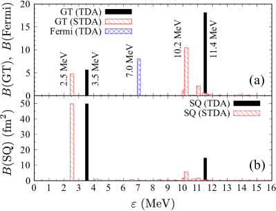
Figure 1: (a) Strength functions of the GT and IAS resonances of ${}^{48}{\rm Ca}$ calculated with the STDA and TDA. The filled and slash-shaded bars are the results of the GT transition calculated with the TDA and STDA, respectively, and the cross-shaded bars are for the IAS resonance. (b) Strength functions of the SQ-1⁺ transition.

To demonstrate our model, we first discuss the Fermi transition measured from the ${}^{48}{\rm Ca}(p,n)^{48}{\rm Sc(IAS)}$ reaction. Figure 1 shows the strength functions of the Fermi and GT transitions of ${}^{48}{\rm Ca}$ calculated with the STDA and TDA. The corresponding excitation energies of the resonance states in question are written explicitly in Fig. 1(a). The TDA calculation gives the $0^{+}$ IAS of ${}^{48}{\rm Sc}$ at $\varepsilon=7.0$ MeV. In the reaction calculation the $Q$ value is calculated with the experimental excitation energy 6.7 MeV Burrows (2006) of the IAS. Note that it is confirmed numerically that the excitation energies of both the TDA and experiment produce identical cross sections.

In addition to the TDA form factor given in Eq. (19), we carry out a phenomenological calculation using the Lane model Lane (1962), which is conventionally adopted to compare theoretical charge-exchange cross section values for the Fermi transition with experimental data. In the Lane model the radial form factor $F_{000}^{s0{\rm(Lane)}}$ is given as the difference of the optical potentials between the final and initial channels:

$$F_{000}^{s0{\rm(Lane)}}(R)=\frac{\left(8\pi T_{A}\right)^{\frac{1}{2}}}{2T_{A}-1}\left[U_{n}^{\rm(N)}(R)-U_{p}^{\rm(N)}(R)\right].$$ (31)

where the phenomenological optical potential Koning and Delaroche (2003) is used.

In Fig. 2, the calculated cross sections of the charge-exchange reaction ${}^{48}{\rm Ca}(p,n)^{48}{\rm Sc(IAS)}$ at incident proton energies $E_{\rm lab}=$ 25, 35, and 45 MeV as a function of the $n$ emitting angle $\theta$ are compared with experimental data Doering et al. (1975); Jon et al. (2000). The cross sections calculated by the TDA (Lane) form factor are shown by the solid (dashed) lines. Note that the theoretical results and experimental data at 35 and 45 MeV are multiplied by $10^{-2}$ and $10^{-4}$, respectively, in order to make them distinguishable from the cross section at 25 MeV.

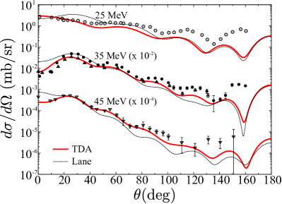
Figure 2: The cross sections of the ${}^{48}{\rm Ca}(p,n)^{48}{\rm Sc(IAS)}$ reaction at $E_{\rm lab}=$ 25, 35, and 45 MeV. The solid lines are the calculated results from the TDA form factor, while the dashed lines are ones from the Lane form factor. The measured data are taken from Refs. Doering et al. (1975); Jon et al. (2000). The lines and the dots are multiplied by $10^{-2}$ ($10^{-4}$) at 35 (45) MeV.

One finds that, in Fig. 2, the results using the TDA form factor reasonably coincide with the experimental angular distribution for 35 and 45 MeV. Although at 25 MeV the TDA result underestimates the data at $\theta\gtrsim 30^{\circ}$, it appears to be better than the Lane model in accounting for the measured behavior. While the Lane model is able to roughly describe the experimental data, it is not as good as the TDA result in the sense of being able to predict the data. It should be mentioned that a different choice of optical potential for the Lane model may improve the prediction of the calculation because its form factor strongly depends on the optical potential used, as reported in Ref. Khoa et al. (2007), for example.

III.3 Spin-flip transitions

We have shown that our framework adequately describes the differential cross section of the ${}^{48}{\rm Ca}(p,n)^{48}{\rm Sc}({\rm IAS})$ reaction. Now we switch gears and investigate the 2p2h effect of the ${}^{48}{\rm Ca}(p,n)^{48}{\rm Sc}(1^{+})$ reaction.

As seen in Fig. 1(a), the GT strengths manifest themselves in two distant regions: one is around 3 MeV, which we refer to as the low-lying resonance, and the other is around 11 MeV, which is nothing but the giant GT resonance. In the STDA, the GT resonance distributes widely due to the 2p2h effect as discussed in Ref. Minato (2016). Note that we choose the most prominent strength from each region of the low-lying and giant GT resonances when calculating the differential cross sections. The strengths of the SQ-$1^{+}$ transition $B({\rm SQ})$, which are the leading part of the $\Delta l=2$ transition, are shown in Fig. 1(b). When we compare cross sections calculated with the STDA and TDA transition densities, the experimental resonance energy of $\varepsilon=2.6$ MeV (11.0 MeV) Yako et al. (2009) is used for the low-lying (giant) resonance. As in the case of the Fermi transition, this slight shift of the $Q$ value from the theoretical one does not vary the calculated cross section significantly; the effect on the cross section at $\theta=0^{\circ}$ is less than 1%.

Let us first focus on the low-lying resonance. Figure 3 shows the differential cross section of the ${}^{48}{\rm Ca}(p,n)^{48}{\rm Sc}$ reaction at $E_{\rm lab}=$ 295 MeV for the low-lying $1^{+}$ resonance as a function of $\theta$ up to $40^{\circ}$. The cross section calculated by the DWBA with the STDA-transition density is indicated by the solid line, whereas the cross section calculated with the TDA is represented by the dashed line. Here the theoretical cross section includes both the GT-type and $\Delta l=2$ transitions.

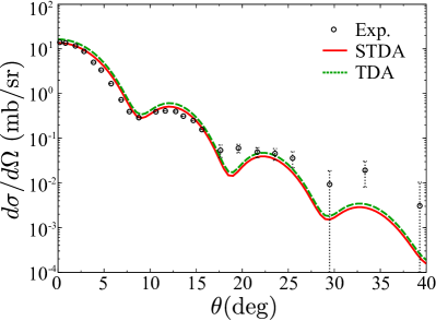
Figure 3: The differential cross section of the ${}^{48}{\rm Ca}(p,n)^{48}{\rm Sc(GT)}$ reaction at $E_{\rm lab}=$ 295 MeV for the low-lying $1^{+}$ resonance state. The calculated result with (without) the 2p2h configuration shown by the solid (dashed) line is compared with the experimental data (open circle) taken from Ref. Yako et al. (2009).

Our calculation reproduces the diffraction pattern of the measured cross section reasonably well for both the STDA and TDA. A difference can be observed only in terms of the magnitude between them. Using the same value of $\bar{V}_{1}$ for the TDA and STDA, the cross sections at $\theta=0^{\circ}$ of the TDA are higher than those of the STDA by about 20%, and the difference remains almost the same for other angles.

The reductions of the cross section by the 2p2h configuration within the STDA are associated with the reduction of $B({\rm GT})$, $B({\rm SQ})$, and so on. We obtained $B({\rm GT})=4.726$ for the STDA and 5.681 for the TDA as shown in Fig. 1(a). The missing strength is brought to a higher energy region Minato (2016). The difference of $B({\rm GT})$ between the TDA and STDA is approximately 20% and is equivalent to the reduction due to the 2p2h effect on the cross section. This proportionality is consistent with the conclusion by Taddeucci et al. Taddeucci et al. (1987) although they neglect the $\Delta l=2$ transition. This fact implies that these contributions are negligibly small (this point will be addressed later).

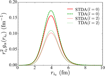
Figure 4: The transition density of the low-lying $1^{+}$ resonance state of ${}^{48}{\rm Sc}$ calculated with the STDA (thick solid line for $l=0$, thin solid line for $l=2$) and TDA (thick dashed line for $l=0$, thin dashed line for $l=2$).

We plot the transition density $g_{\alpha}$ in Fig. 4 to investigate the difference in the calculated cross sections of the TDA and STDA in detail. The thick (thin) solid and thick (thin) dashed lines are respectively the results of the STDA and TDA for $l=0$ ($l=2$) corresponding to the GT ($\Delta l=2$) transition. One finds the difference in the amplitudes of the transition density between the STDA and TDA. Taking the ratio of the STDA amplitude for $l=0$ at the peak around $r_{i_{t}}\sim 4$ fm with the similar amplitude calculated from the TDA, we obtain $0.156/0.173\sim 0.902$. Because $B({\rm GT})$ is proportional to $g^{2}_{\alpha}$, one obtains $(0.902)^{2}=0.814$, which is consistent with the reduction of $B({\rm GT})$.

Table 1: Leading configurations of the $1^{+}$ resonance and its amplitude defined by $X_{mi}^{2}$ of the 1p1h states calculated by the TDA and STDA are listed. The 2p2h amplitude $P_{\rm 2p2h}$ is calculated by $P_{\rm 2p2h}=\sum_{mnij}\mathcal{X}_{mnij}^{2}$.

	Configuration	TDA	STDA
Low-lying GT	$\pi(1f_{7/2})\nu(1f_{7/2})^{-1}$	0.954	0.858
	$\pi(1f_{5/2})\nu(1f_{7/2})^{-1}$	0.043	0.047
	$\pi(2f_{7/2})\nu(1f_{7/2})^{-1}$	0.001	0.001
	$P_{\rm 2p2h}$	0.000	0.091
Giant GT	$\pi(1f_{7/2})\nu(1f_{7/2})^{-1}$	0.042	0.043
	$\pi(1f_{5/2})\nu(1f_{7/2})^{-1}$	0.950	0.483
	$\pi(2f_{5/2})\nu(1f_{7/2})^{-1}$	0.004	0.002
	$P_{\rm 2p2h}$	0.000	0.470

The diffraction pattern of the cross section has a sensitivity to the shape of the transition density rather than its amplitude because the angular distribution is determined by the region where the incident proton interacts with the target nucleus. In Fig. 4, the STDA and TDA lines have a similar $r_{i_{t}}$ dependence for each $l$. Inclusion of the 2p2h configuration does not significantly change the shape of the transition density although the amplitudes are about 10% (7%) smaller for the TDA for $l=0$ $(l=2)$. In Table 1, the 1p1h configurations contributing to the low-lying GT resonance and its amplitude defined by $X_{mi}^{2}$ are listed. The main configurations are $\pi(1f_{7/2})\nu(1f_{7/2})^{-1}$ and $\pi(1f_{5/2})\nu(1f_{7/2})^{-1}$ for both the TDA and STDA. While the amplitude of $\pi(1f_{5/2})\nu(1f_{7/2})^{-1}$ is almost the same for both, the amplitude of $\pi(1f_{7/2})\nu(1f_{7/2})^{-1}$ for the STDA is about 0.1 smaller than that for the TDA. This difference might change the shape of the transition density if the radial dependences of the wave functions of $\pi(1f_{7/2})$ and $\pi(1f_{5/2})$ are different. However, they are almost the same because they are spin-orbit partners. Therefore, unless another configuration intervenes, the shape of the transition density will not change significantly. As a consequence, we obtained differential cross sections of similar shape for the STDA and TDA.

Figure 5 shows the cross sections calculated with $g_{s1}$ and $g_{l2}$ (solid line), only with $g_{s1}$ (dashed line), and only with $g_{l2}$ (dotted line) by means of the STDA, as well as experimental data Yako et al. (2009) (open circle). Throughout the observed region of $\theta$, the result including only the $\Delta l=2$ transition is about two orders smaller than the others. At $\theta=0^{\circ}$, in particular, it is about five orders smaller than that of GT alone even though $r_{i_{t}}^{2}g_{l2}$ has a peak amplitude about 36% smaller than that of $r_{i_{t}}^{2}g_{s1}$ (see Fig. 4). It indicates that there are dynamical processes such as angular-momentum coupling coefficients and coherent summation in Eq. (24), which hinder the $\Delta l=2$ components, and thus the effect of the $\Delta\l=2$ transition on the transition density does not coincide quantitatively with that observed on the cross section.

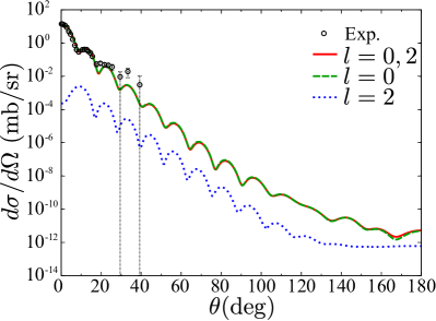
Figure 5: The cross section of ${}^{48}{\rm Ca}(p,n)^{48}{\rm Sc}$ at 295 MeV for the low-lying $1^{+}$ resonance state calculated with the STDA transition density of the GT and $\Delta l=2$ transitions (solid line), the GT transition only (dashed line), and $\Delta l=2$ transition only (dotted line).

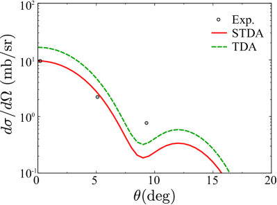
Figure 6: Same as Fig. 3 but for the giant resonance.

Next we discuss the 2p2h effect on the giant GT resonance. In Fig. 6 the lines and open circles are defined in the same way as in Fig. 3 but for the giant resonance with $\theta$ up to $20^{\circ}$. The result of the STDA reasonably traces the first two points of the experimental data, but fails for the third one. By the 2p2h effect, the cross section of the STDA is smaller than that of the TDA by about 43% at $\theta=0^{\circ}$ but does not change its shape significantly. Again, comparing $B({\rm GT})$ of the STDA and TDA shown in Fig. 1(a), the 2p2h effect on $B({\rm GT})$ of the giant resonance is about a 42% reduction, which agrees with the value of its effect on the cross section.

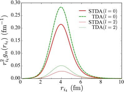
Figure 7: Same as Fig. 4 but for the giant resonance.

Figure 7 shows the transition density of the giant resonance. From the difference between the STDA and TDA, we find that the 2p2h configuration reduces the amplitude of $r_{i_{t}}^{2}g_{\alpha}$ at the peak position around $r_{i_{t}}=4$ fm by about 25% (43%) for $l=0$ ($l=2$). As we did in the low-lying resonance, calculating the squared ratio of the amplitude of the STDA to that of the TDA, one obtains $(0.211/0.281)^{2}\sim 0.564$, which is almost consistent with the reductions of $B(\rm{GT})$ and the cross section. From Table 1, the 1p1h configurations mainly contributing to the giant GT resonance are $\pi(1f_{7/2})\nu(1f_{7/2})^{-1}$ and $\pi(1f_{5/2})\nu(1f_{7/2})^{-1}$ both for the TDA and STDA, as in the case of the low-lying resonance. While the amplitude of $\pi(1f_{7/2})\nu(1f_{7/2})^{-1}$ almost remains the same for both the TDA and STDA, that of $\pi(1f_{5/2})\nu(1f_{7/2})^{-1}$ for the STDA is half of that for the TDA. However, this difference does not make a significant change in the shape of the transition density and accordingly in the diffraction pattern of the cross section, similar to the low-lying resonance, as seen in Fig. 6.

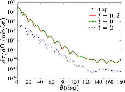
Figure 8: Same as Fig. 5 but for the giant resonance.

Figure 8 shows the cross section at the giant GT resonance. The result of $\Delta l=2$ transition only is negligibly small as compared to the others. It is about two orders smaller than the GT transition in $\theta>0$, and the ratio of their cross sections at $\theta=0^{\circ}$ is approximately $10^{-5}$, similar to the result of the low-lying resonance.

As a consequence, qualitatively the 2p2h effect reduces the amplitude of the cross section but does not change the diffraction pattern. The values of the decrease on the cross section due to the 2p2h configuration are essentially consistent with those obtained from the structural calculation.

Last, we comment on the tensor-force contribution, which was reported Minato (2016) to change the excitation energy of the spin-flip resonance states and the corresponding $B({\rm GT})$ values. However, we have confirmed numerically that the inclusion of the tensor force does not change the diffraction pattern of the cross section.

IV Summary

The charge-exchange reaction ${}^{48}{\rm Ca}(p,n)^{48}{\rm Sc}$ has been investigated theoretically to clarify the effect of 2p2h-configuration mixing on the GT-resonance states. We have carried out the STDA calculation in order to prepare the transition density, and the form factor has been obtained by employing the phenomenological nucleon-nucleon interaction. The angular-distributed cross section has been computed by means of the DWBA with the microscopic form factor.

The Fermi transition has also been calculated to demonstrate the effectiveness of our framework. The calculated cross sections of the Fermi transition caused by the ${}^{48}{\rm Ca}(p,n)^{48}{\rm Sc(IAS)}$ reaction at $E_{\rm lab}=$ 25, 35, and 45 MeV coincide well with the measured data Doering et al. (1975); Jon et al. (2000).

It has been found that the 2p2h effect on the cross section of the ${}^{48}{\rm Ca}(p,n)^{48}{\rm Sc}$ reaction at 295 MeV decreases the amplitude of the cross section and does not change the angular distribution for either the low-lying or giant resonances. This feature is consistent with the result of the structural calculation. However, the 2p2h effect on the angular distribution may become important for other multipole transitions because it was reported that the transition densities of the isovector monopole and the quadrupole of ¹⁶O were changed significantly Gambacurta et al. (2010). Quantitatively, the reduction of the cross section due to the 2p2h effect can be explained by that of $B({\rm GT})$ and the corresponding transition density.

The role of the $\Delta l=2$ transition on $1^{+}$-resonance states has also been surveyed and found to give a negligibly small contribution. It supports the proportion relation Taddeucci et al. (1987) between $B({\rm GT})$ and the charge-exchange cross section at zero degree. Note that, in our model, the form factor of the $\Delta l=2$ transition has been calculated using the same nucleon-nucleon interaction as that of the GT transition. A different nucleon-nucleon interaction should be tested, for example, the $t$ matrix of Franey and Love Franey and Love (1985) or the $g$ matrix of Jeukenne-Lejeune-Mahaux Jeukenne et al. (1977), as adopted in previous studies Taddeucci et al. (1987); Kerman et al. (1959); Bertsch and Esbensen (1987); Khoa et al. (2007).

A systematic comparison of the reaction models such as the DWBA, DWIA, and coupled-channels method for the charge-exchange reaction at several incident energies with several target nuclei will provide important guidance for analyses of experimental data.