CLIMEX: A Wireless Physical Layer Security Protocol Based on Clocked Impulse Exchanges

Abstract

A novel method and protocol establishing common secrecy based on physical parameters between two users is proposed. The four physical parameters of users are their clock frequencies, their relative clock phases and the distance between them. The protocol proposed between two users is backed by theoretical model for the measurements. Further, estimators are proposed to estimate secret physical parameters. Physically exchanged parameters are shown to be secure by virtue of their non-observability to adversaries. Under a simplified analysis based on a testbed settings, it is shown that $38$ bits of common secrecy can be derived for one run of the proposed protocol among users. The method proposed is also robust against various kinds of active timing attacks and active impersonating adversaries.

I Introduction

Clocks are everywhere. They are found in every gadget around us. Various operations across the digital system are synchronized at clock edges. Crystal clocks are used in most consumer electronics present in our surroundings as heart beats of electronic systems. This motivates usage of physical characteristics of clocks in security applications and has the potential to provide security to far reaches of electronic presence.

Ever present electronics with clocks is synonymous to internet-of-things (IOT) context. With increasing potential of IOT applications, security of data exchange in IOT applications also is of paramount importance [1, 2]. The IOT context puts more stringent constraints on resource consumption for achieving secrecy. Low complexity schemes for key generation is proposed in [3] As suggested in [4], physical layer security can play an important role in IOT applications by alleviating the need for high computation required in traditional cryptography by making use of existing radio functionality to support security. In [5], involvement of control and physical layer of a system for security of cyber physical system (CPS) is suggested. In physical layer security, encrypting messages using secret keys generated based on wireless channel is the most investigated method [4, 6, 7, 8, 9, 10, 11, 12]. In an Alice, Bob and Eve setup as shown in Fig.1, secret key generation has been based on the uniqueness of channel between Alice and Bob than Alice-Eve or Bob-Eve channel. Most of above wireless based key generation methods rely on randomness of channel to produce a unique key between Alice and Bob. However, such schemes suffer from many weaknesses as discussed in [4]. Assumptions such as Gaussian symmetric channel, dynamic requirement of the channel, weak adversary models etc. are shown to be weak on many instances. Many other practical implementation and usage issues in implementing wireless channel based physical layer security are discussed in [10, 4].

A few other physical parameters are proposed for generating secret keys over wireless. They are received signal strength (RSS), drifting oscillators, distance between nodes, radiometric signatures, quantum key generation etc [13, 14, 15, 16, 17, 18, 19]. In [13], exhaustive review on key generation from physical parameters are written. Various ways of non-cryptographic authentication are described.

Figure 1: Alice, Bob and Eve setup. Alice and Bob separated by distance $\rho_{\text{\tiny AB}}$ exchange physical parameters over wireless to generate a shared secret key. Eve who is $\rho_{\text{\tiny AE}}$ distance away from Alice and $\rho_{\text{\tiny BE}}$ away from Bob, is an adversary listening to the wireless exchanges. She is attempting to decipher the parameters from measurements.

In [15], effectiveness of RSS for secret key generation between two nodes is experimentally analysed and in absence of a highly dynamic environment, low entropy bits are generated for secret keys. The randomness of a physical clock parameter, i.e., its oscillating frequency has been suggested a few times [20, 21, 22]. A carrier frequency tracking framework and subsequent device authentication based on it is proposed in [20]. Whereas, a multi-input multi-output (MIMO) device authentication based on carrier frequencies from all the transmitters is proposed in [22]. The papers suggesting oscillator properties for secure exchanges are mostly based on authenticating nodes by their signature oscillator characteristics. These papers mostly describe the system to the extent of proving uniqueness of absolute or relative oscillator characteristics, while having a weak or no adversary model assumptions. Security in clock synchronization schemes has also been discussed [23, 24]. Usage of clock synchronization to detect man-in-the-middle attack is discussed in [25]. Fundamental limits on security using clock synchronization is proposed along with clock synchronization protocol for security purposes. Among other contexts of physical layer security, physical layer security in sensor networks based on distributed detection have been recently discussed in [3, 26].

Usage of distance and position for securing communication has often been discussed [13, 14, 15, 27, 28, 29, 30]. Usage of distance between nodes implicitly appears in RSS based authentication and secure key generation methods [13, 14, 15]. Whereas, explicit application of distance for security appears in concepts such as distance bounding protocols and their use in concepts such as secure neighbourhod discovery [18, 28, 29, 31, 32, 33].

Vulnerability to active adversaries has been a very critical issue in secure communications and key exchanges [34, 35, 36, 37, 27]. There is limited discussion on active adversary in physical layer context as pointed out in [34]. In this paper usage of the proposed method in warding off adversary attack is also suggested. Various active adversary models are suggested in [27] which are very relevant to this work and considered in subsequent sections of the paper.

The main motivation of this paper is proposing a secure mechanism to exchange physical parameters of users among them over wireless. Accordingly, the main idea proposed in this paper is a protocol which helps in secret exchange of physical parameters between two nodes. The proposed protocol and the measurements based on the protocol lets two nodes exchange their relative physical parameters. The protocol incorporates actions at two nodes to strengthen the robustness of parameter exchange against any passive eavesdropper and to some extent to an active adversary, as explained later in the paper. The protocol exploits a physical phenomena between two continuous running clocks separated by a distance for parameter exchange while providing secrecy.

Any two physical clocks can have a frequency and a phase relation. The frequency relation considered here is the difference in frequency ($f_{d}$) between the clocks and the phase relation ($\phi$) is the relative phase of the clocks. If these clocks are mounted on two separate devices then the distance between these user ($\rho$) provides another physical dimension to use. Further in the paper, a set of four independent parameters i.e., two clock frequencies of users derived from difference frequencies, their relative phase and the distance between them are shown to be exchanged as shared secret parameters between two users. The idea presented in this paper is outcome of experiments with impulse radio ultrawideband (IR-UWB) testbed [38, 39] that manifests practical relevance of the work.

In this paper IR-UWB signals are suggested to be used for signalling among Alice and Bob in Fig.1. Alice periodically sends Ping signals to Bob and after a delay Bob sends a Respond signal. The nodes Alice and Bob exchange impulse signals Ping and Respond triggered by time events generated using an oscillator or a clock. Hence the mechanism or the protocol of signal exchange will be called as CLocked IMpulse EXchange (CLIMEX). Further discussions in the paper is based on classical Alice, Bob and Eve setup [7, 8].

The main contributions of the paper are:

1. The CLIMEX protocol between two nodes to exchange physical parameters of two nodes discreetly over wireless.

2. A mathematical model for the measurements at nodes.

3. Estimators for estimating required parameters at nodes from the collected measurements.

4. A simplified analysis to evaluate number of possible secret bits which can be derived from epochs of measurements. Secret bits derived can be further used for encryption and authentication.

5. Evaluation in presence of passive adversary. Different possible measurements by passive adversary are considered in this paper.

6. Discussing robustness against a few types of active adversaries. Particularly, against timing attacks and impersonating adversary.

Figure 2: Conceptual timing diagram of one-way RTT protocol between Alice and Bob. Alice transmits Ping at interval $T_{m}$ seconds and collects measurements $\left[y_{\text{\tiny A}}(1)\ y_{\text{\tiny A}}(2)\cdots\right]^{\top}$. Bob is a distance $\rho_{\text{\tiny AB}}$ away from Alice and sends Respond after a delay $\delta_{\text{\tiny B}}$ from the instance it receives the Ping from Alice.

In summary, we propose analyse and provide experimental observations for CLIMEX as a tool for secure exchange of physical parameters.

This paper is organised as follows. Section II describes the principle of operation, gives an overview of measurements, describes the basic phenomenon to be used and introduces the CLIMEX protocol while comparing it with the basic RTT protocol. Section II describes the basic scheme and compares the proposed CLIMEX protocol with basic RTT protocol. Next described are measurement models for the protocols in section III. Estimators based on measurement models are presented in IV. Following estimators is the section V-B on adversary models which discusses possible measurements adversary can do. Section V has analyzed the security aspects proposed in this paper. It is followed by further discussion on practicality and possible future work on the proposed idea in section VI. The last section then is the conclusion.

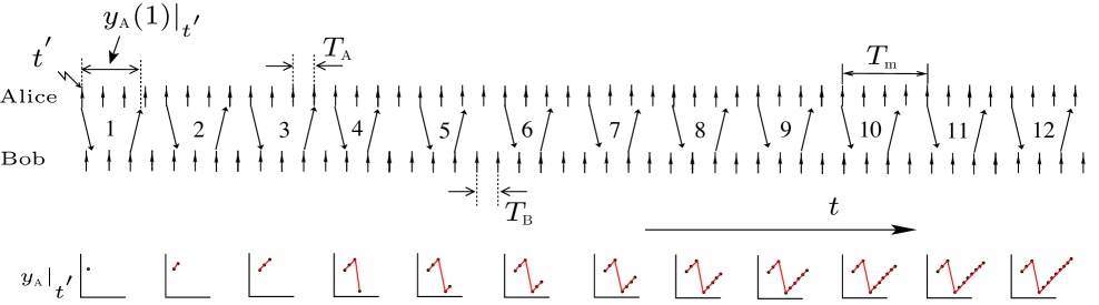
Figure 3: Interplay between two clocks giving rise to sawtooth measurements at the measuring end.

II Principle of Operation

The principle of parameter exchange among nodes proposed in this paper is based on round trip time (RTT) measurements. One-way RTT is shown in the Fig.2. Alice sends ’Ping’ signals to Bob at regular interval of $T_{m}$ seconds. Bob responds after a delay $\delta_{\text{\tiny B}}$ and does not collect any measurement. The delay $\delta_{\text{\tiny B}}$ is generated at Bob’s end using its own clock with frequency $f_{\text{\tiny B}}$. Alice collects an epoch of RTT measurements, $\left[y_{\text{\tiny A}}(1)\ y_{\text{\tiny A}}(2)\cdots\right]^{\top}$. These measurements are collected using a precise time difference measurement device which usually has time measurement precision much higher than clock periods of the clocks in discussion. For very clock frequencies (MHz or greater) in consideration, typically the precision is in range of nano to pico seconds. One such device is time to digital converter (TDC) [40, 41]. Usage of such measurement precision is also customary in network time synchronization schemes like precision time protocol (PTP) [42, 43]. It is followed by Bob also collecting an epoch of measurements $\left[y_{\text{\tiny B}}(1)\ y_{\text{\tiny B}}(2)\cdots\right]^{\top}$ by sending several ’Pings’ and measuring RTT where Alice introduces delay $\delta_{\text{\tiny A}}$ using its clock with frequency $f_{\text{\tiny B}}$.

From their wireless signal exchanges and RTT measurements, Alice and Bob can estimate a few relative parameters among them. They can estimate their relative clock frequency $f_{d}=f_{\text{\tiny A}}-f_{\text{\tiny B}}$, relative phase of their clocks, $\phi_{\text{test}}$ and the parameter $\rho_{\text{\tiny AB}}$, the distance between Alice and Bob [38, 39]. The first measurements at Alice in the sequence of measurements is timestampped with time $t^{{}^{\prime}}$. The phase of the signal in the measurement depends on the instance of the measurement collection. It is assumed that the physical parameters to be exchanged remain time invariant during this period when Alice and Bob collect their respective measurements.

II-A Interplay between two clocks

As shown in Fig.3, Alice and Bob periodically exchange Pings and corresponding Responds. Figure 3 illustrates generation of sawtooth waveform as a result of interplay between clocks of Alice and Bob through RTT measurements among them. Alice’s clock has period $T_{\text{\tiny A}}=1/f_{\text{\tiny A}}$ and Bob’s clock has period $T_{\text{\tiny B}}=1/f_{\text{\tiny B}}$. Alice sends successive Pings at regular interval, $T_{\text{\tiny m}}=4T_{\text{\tiny A}}$ in the illustration. Bob Responds after introducing a delay of one clock period $T_{\text{\tiny B}}$ from the clock edge subsequent to arrival of signal from Alice. As illustrated form the figure, at instance 3, Bob receives Ping from Alice just after a clock edge has elapsed, which results in largest RTT measurement at Alice. Whereas, at instance 4, Bob receives the Ping nearly at the same time a clock edge arrives. Hence, the RTT at Alice is the smallest. The frequency of sawtooth waveform is the difference frequency $f_{d}$. The height of the sawtooth measurement equals $T_{\text{\tiny B}}$. The phase of both clocks are related to the phase of the sawtooth waveform which is a function of $t^{{}^{\prime}}$, instance when the measurement begins. Generation of sawtooth from RTT measurements was first reported in [39]. The above protocol of signal exchange between Alice and Bob is RTT protocol. CLIMEX protocol with a few changes in RTT protocol is introduced next.

(a) The RTT protocol.

(b) The CLIMEX Protocol.

Figure 4: The RTT protocol and the CLIMEX protocol. In addition to the RTT protocol, the CLIMEX protocol has random transmission delays $\Delta_{1}$, $\Delta_{2}$ introduced by Alice and scaled delay $\bar{\delta}_{\text{\tiny B}}(1)$ at Bob’s end.

II-B RTT protocol and the CLIMEX protocol

RTT measurements where events are initiated by clock edges at both the ends are shown in Fig.4. The figure has clock tick level detail of RTT measurements shown in Fig.2. Figure 4(a) is the RTT protocol resulting in sawtooth RTT measurements and Fig.4(b) is the CLIMEX protocol. RTT and CLIMEX protocols are explained now.

1. The upside arrows in the Figs. 4(a) and 4(b) are the clock edges(ticks) of Alice’s and Bob’s clocks. As in the Fig.4(a), Ping and Respond events are generated on clock edges.

2. Alice transmits Ping signals periodically every $T_{m}$ seconds. Alice counts this period using its clock with clock period $T_{\text{\tiny A}}$. In the CLIMEX protocol of Fig. 4(b), instead of transmitting Ping at clock edge, Alice transmits after a random delay $\Delta_{1}$ from the clock edge. The added random delay is known only to the Alice. It provides secure exchange of keys by dithering RTT measurements as explained later in III-B.

3. Bob receives the Ping after a path delay of $\rho_{\text{\tiny AB}}/c$ seconds, $c$ is speed of light. In the RTT protocol of Fig.4(a), Bob responds to Alice’s ping after a nominal wait, $\delta_{0}$, of two clock periods. The total delay at Bob’s end would be $\delta_{\text{\tiny B}}(1)$. In the CLIMEX protocol, Bob responds to Alice’s Ping after a scaled delay of $\bar{\delta}_{\text{\tiny B}}(1)$ seconds as shown in Fig.4(b). The scaled delay $\bar{\delta}_{\text{\tiny B}}$ will be explained in III-B.

4. Alice receives Bob’s Respond and measures RTT $y_{\text{\tiny A}}(1)$ as shown in Figs. 4(a) and 4(b).

5. Alice collects an epoch of $N$ RTT measurements. Measurements are timestampped by time measurement beginning, $t^{\prime}$. $\mathbf{y_{\text{\tiny A}}}|_{t^{\prime}}=[y_{\text{\tiny A}}(1)\cdots\>y_{\text{\tiny A}}(N)]^{\top}\in\mathbb{R}^{N}$.

6. After Alice, Bob collects his measurements in a similar way as Alice. Bob’s epoch of measurements is $\mathbf{y_{\text{\tiny B}}}|_{t^{\prime\prime}}=[y_{\text{\tiny B}}(1)\cdots\>y_{\text{\tiny B}}(N)]^{\top}\in\mathbb{R}^{N}$ which is timestampped by $t^{\prime\prime}$.

As evident from the above discussion that the main differences between the RTT protocol and the CLIMEX protocol are addition of random delay $\Delta_{i}$ to Pings by Alice and the scaled Respond $\bar{\delta}_{\text{\tiny B}}$ by Bob. In the next section it will be shown that the proposed changes to the CLIMEX protocol over RTT protocol gives rise to a measurement model which helps in establishing common secrecy between Alice and Bob.

III Measurement Model

In this section, measurement model of RTT protocol as shown in Fig.4(a) and CLIMEX protocol as shown in Fig.4(b) is suggested. As subsequently shown, both the measurement model is nonlinear in parameters of interest and model of CLIMEX protocol provides useful features for secure exchanges of parameters.

III-A Measurement model for an epoch collection by Alice one-way in RTT protocol

RTT measurement epoch recorded by Alice is $\mathbf{y_{\text{\tiny A}}}|_{t^{\prime}}=[y_{\text{\tiny A}}(1)\cdots\>y_{\text{\tiny A}}(N)]^{\top}\in\mathbb{R}^{N}$. It can be written compactly in vector form as

$$\mathbf{y_{\text{\tiny A}}}|_{t^{\prime}}=\boldsymbol{\delta}_{\text{B}}+\frac{2\rho_{\text{\tiny AB}}}{c}\mathbf{1}+\mathbf{w}\,,$$ (1)

where $\boldsymbol{\delta}_{\text{B}}$ is the total delay vector at Bob’s node

$$\boldsymbol{\delta}_{\text{B}} = \mathbf{h}(f_{d},T_{\text{\tiny B}},\phi^{{}^{\prime}},\mathbf{n})+\delta_{0}\mathbf{1}.$$ (2)

The function $\mathbf{h}(f_{d},T_{\text{\tiny B}},\phi^{{}^{\prime}},\mathbf{n})=[h(1)\cdots\>h(N)]^{\top}$ results in sawtooth shape in measurements and can be given by

$$\mathbf{h}(f_{d},T_{\text{\tiny B}},\phi^{{}^{\prime}},\mathbf{n})\triangleq\text{mod}_{T_{\text{\tiny B}}}\Bigg{(}\!\frac{\displaystyle T_{\text{\tiny B}}}{\displaystyle 2\pi}\text{mod}_{2\pi}(2\pi f_{d}\mathbf{t}+\phi^{{}^{\prime}}\mathbf{1})+\mathbf{n}\!\Bigg{)}.$$ (3)

The time vector $\mathbf{t}=[t^{\prime}\ t^{\prime}+T_{m}\ t^{\prime}+2T_{m}\ \cdots\ t^{\prime}+(N-1)T_{m}]^{\top}$. $\phi^{{}^{\prime}}$ is the relative phase of Alice’s and Bob’s clock when the measurement has timestamp $t^{\prime}$ with first measurement $y_{\text{\tiny A}}(1)$. Similarly, $\phi^{{}^{\prime\prime}}$ is the phase of sawtooth where the measurement epoch is collected by Bob. The noise vectors $\mathbf{n}$ and $\mathbf{w}$ are explained in detail in the subsection III-C.

There are two modulus terms in (6). The internal modulus is with respect to $2\pi$ radians which corresponds to one period of the sawtooth waveform [39]. The outer modulus is taken with respect to $T_{\text{\tiny B}}$. The outer modulus was not considered before as $\sigma^{2}_{j}$ and $\sigma^{2}_{c}$ were assumed small [39]. The model with only internal modulus was accurate enough to estimate parameters of interest with sufficient accuracy from the experimental data. However, in the current paper, random delays ($\Delta_{i}$) are added to the argument of the outer modulus. Hence the outer modulus comes into picture. Explanation for outer modulus is seen from Fig.5(a) which is a phasor diagram for argument of the sawtooth measurement. A noise term $n_{j}$ can move a phasor from one quadrant to another. Such transitions of moving a signal to the first quadrant results in nonlinear jumps in sawtooth waveform at discontinuities, as shown in Fig.5(a). Also shown in the figure are effect of the phasor jump on RTT measurements. ’RTT noiseless’ is RTT without any noise. Whereas, ’RTT with noise’ is the RTT measurement when noise appears at phase discontinuity of sawtooth waveform. The sawtooth waveforms at Alice for two cases depending on the sign of $f_{d}$ is shown in Fig.5(b) and Fig.5(c). In Fig.5(b), Alice’s clock frequency is larger than Bob and in 5(c), it is smaller. The characteristic sawtooth waveform provides a valid signature to message exchange between Alice and Bob as discussed later.

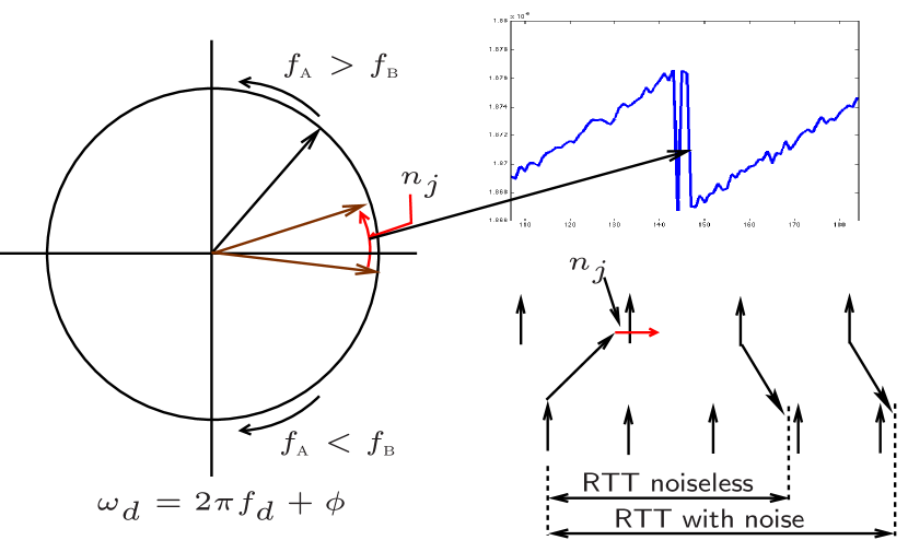
(a) Phasor for sawtooth measurements. Shows noise effect in jumping quadrant leading to zero crossings.

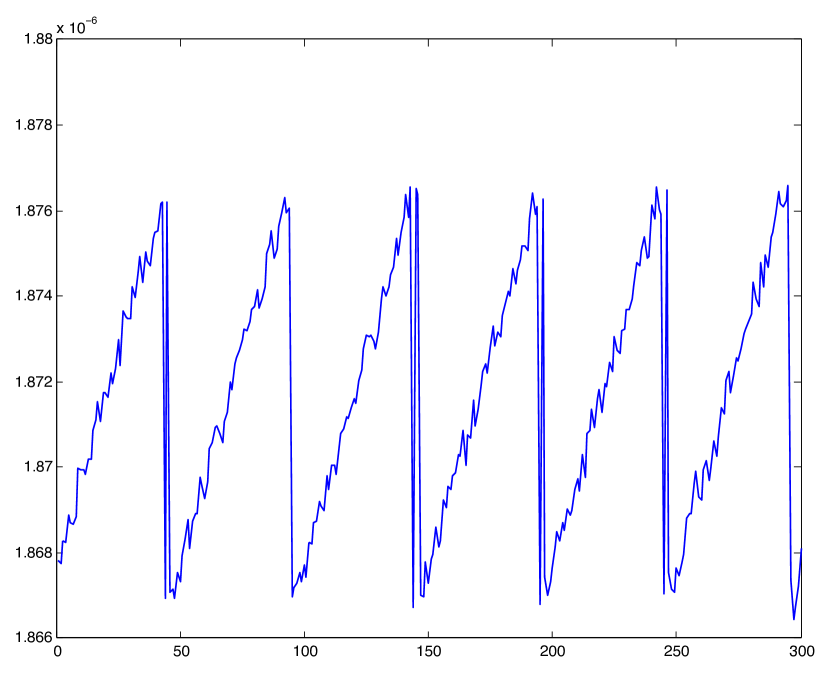
(b) Measurements at Alice/Bob, Sawtooth has positive slope as $f_{\text{\tiny A}}$ is larger than $f_{\text{\tiny B}}$, for $f_{d}=f_{\text{\tiny A}}-f_{\text{\tiny B}}$.

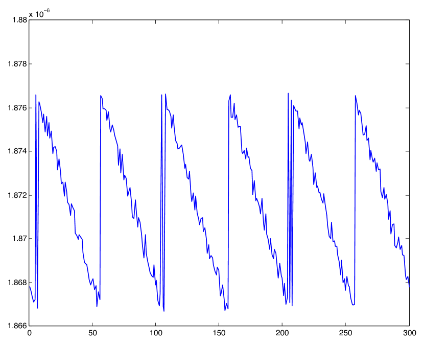
(c) Measurements at Bob/Alice, Sawtooth has negative slope as $f_{\text{\tiny A}}$ is smaller than $f_{\text{\tiny B}}$, for $f_{d}=f_{\text{\tiny A}}-f_{\text{\tiny B}}$.

Figure 5: Details of measurement protocol, phasor argument of the sawtooth function and effect of noise.

(a) $\,\Delta\sim\mathcal{U}(0,0)$

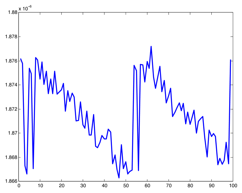
(b) $\,\Delta\sim\mathcal{U}(0,0.25T_{\text{\tiny A}})$

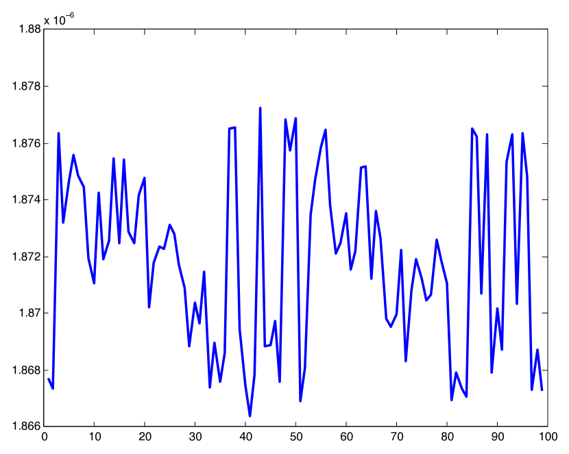
(c) $\,\Delta\sim\mathcal{U}(0,0.5T_{\text{\tiny A}})$

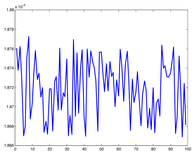
(d) $\,\Delta\sim\mathcal{U}(0,0.75T_{\text{\tiny A}})$

(e) $\,\Delta\sim\mathcal{U}(0,T_{\text{\tiny A}})$

Figure 6: RTT Measurements as a result of added random Ping delays $\mathbf{\Delta}$. As illustrated in the figure, increasing standard deviation of $\mathbf{\Delta}$ increases dithering of measurements. $\mathbf{\Delta}$ is known only to the node transmitting Pings. Any other node doing measurements will not be able to infer any information from it, due to lack of any information about $\mathbf{\Delta}$.

III-B Measurement model for an epoch collection by Alice in CLIMEX protocol

RTT measurements recorded by Alice after running CLIMEX protocol with Bob as shown in Fig.4(b) can be written

$$\mathbf{y_{\text{\tiny A}}}|_{t^{\prime}}=\boldsymbol{\bar{\delta}}_{\text{B}}+\frac{2\rho_{\text{\tiny AB}}}{c}\mathbf{1}+\mathbf{w}\,,$$ (4)

where $\boldsymbol{\bar{\delta}}_{\text{B}}$ is the total delay vector at Bob’s node,

$$\boldsymbol{\bar{\delta}}_{\text{B}} = \mathbf{g}(f_{d},A,\phi^{{}^{\prime}},\mathbf{\Delta},\mathbf{n})+\delta_{0}\mathbf{1}.$$ (5)

The function $\mathbf{g}(f_{d},A,\phi^{{}^{\prime}},\mathbf{n})=[g(1)\cdots\>g(N)]^{\top}$ results in sawtooth shape in measurements. The function $\mathbf{g}(f_{d},T_{\text{\tiny B}},\phi^{{}^{\prime}},\mathbf{\Delta},\mathbf{n})$ in this case is

$$\mathbf{g}(f_{d},A,\phi^{{}^{\prime}},\mathbf{\Delta},\mathbf{n})$$

$$\!\!\!\!\!\!\!\!\!\triangleq\frac{A}{T_{\text{\tiny B}}}\text{mod}_{T_{\text{\tiny B}}} \!\!\!\!\!\Bigg{(}\frac{\displaystyle T_{\text{\tiny B}}}{\displaystyle 2\pi}\text{mod}_{2\pi}(2\pi f_{d}\mathbf{t}+\phi^{{}^{\prime}}\mathbf{1})+\mathbf{\Delta}+\mathbf{n}\Bigg{)}\,.$$ (6)

In (6), $\mathbf{\Delta}$ is the random delay vector, $\mathbf{\Delta}=[\Delta_{1},\Delta_{2},...,\Delta_{N}]^{\top}$. Delay $\Delta_{1}$ shown in Fig.4(b) is known only to Alice and can be assigned any distribution in order to increase estimation error of parameters at Eve. Figure 6 shows RTT measurements at Alice when random transmission delay uniformly distributed between is $0$ and $T_{\text{\tiny A}}$ are added while sending Pings. The figure shows the dithering effect delays $\mathbf{\Delta}$ have on RTT measurements. Figure 6(a) corresponds to measurements with no random delay added to Pings and the measurement has the sawtooth waveform. In subsequent figures 6(b), 6(c), 6(d) and 6(e) increasing variance of the added random delay increasingly distorts the measurement waveforms. Alice can estimate the shared secret parameters these measurements with the knowledge of $\mathbf{\Delta}$ as will be discussed in next section while discussing estimators for these parameters. Whereas, the adversary Eve can not infer parameters from these measurements without the knowledge of delays $\mathbf{\Delta}$.

As it can be seen from (3), the outer modulus with respect to $T_{\text{\tiny B}}$ will have a peak-to-peak magnitude of $T_{\text{\tiny B}}$. The height of the sawtooth reveals information on Bob’s clock period in such measurements. As can be seen further in the discussion from (14) that Eve can estimate parameters of sawtooth from TDOA measurements while eavesdropping. Thus an eavesdropper to the RTT measurements can estimate Bob’s clock period $T_{\text{\tiny B}}$, hence clock frequency $f_{\text{\tiny B}}$. To avoid this, as explained in section II-B, time scaling of the delay by Bob is proposed before sending Respond. As shown in the Fig.7, delay $\delta_{\text{\tiny B}}$ with maximum value $T_{\text{\tiny B}}$ seconds is scaled to a delay $\bar{\delta}_{\text{\tiny B}}$ with maximum value $A$ seconds.

Figure 7: Delay scaling at responding node Bob. The actual delay $\delta_{\text{\tiny B}}$ is mapped to the delay $\bar{\delta}_{\text{\tiny B}}$ to ensure the maximum height of sawtooth is ’$A$’.

$$\bar{\delta}_{\text{\tiny B}}=\delta_{\text{\tiny B}}\frac{A+\delta_{0}}{T_{\text{\tiny B}}+\delta_{0}}.$$ (7)

$A$ is known to all. As shown in Fig.4(b), Bob measures $g(1)$ and computes $\delta_{\text{\tiny B}}=g(1)+\delta_{0}$. Further, Bob computes $\bar{\delta}_{\text{\tiny B}}$ from (7) and advances or delays transmitting Respond by $\delta_{\text{\tiny B}}\pm\bar{\delta}_{\text{\tiny B}}$ seconds. In the shown examples of Fig.4(b) and Fig.7, $A$ is shown smaller than $T_{\text{\tiny B}}$. Hence Bob is shown advancing the time of Respond transmission. With scaled Respond, the sawtooth function (3) in RTT protocol transforms with a multiplicative factor $\frac{A}{T_{\text{\tiny B}}}$ as (6) in the CLIMEX protocol. As a result, peak-to-peak amplitude of the sawtooth in CLIMEX protocol is a known to all value $A$.

III-C The noise model

There are two sources of noise in CLIMEX protocol. One is jitter noise in clock edges of Alice and Bob with assumed distribution $\mathcal{N}(0,\sigma^{2}_{j})$ and another is channel noise from wireless transmission with distribution $\mathcal{N}(0,\sigma^{2}_{c})$. In measurement models, (1), (2), (3), (4), (5) and (6), the noise vector $\mathbf{n}$ consists of noises generated from from Alice’s clock noise while transmitting Ping, wireless channel and Bob’s clock noise in starting the delay generation subsequent to receiving Ping. Hence, $\mbox{cov}(\mathbf{n})=(\sigma^{2}_{c}+2\sigma^{2}_{j})\mathbf{I}$. Similarly, the noise vector $\mathbf{w}$ consists of noises from Respond generation and wireless channel. Hence, $\mbox{cov}(\mathbf{w})=(\sigma^{2}_{c}+\sigma^{2}_{j})\mathbf{I}$.

Figure 8: Alice predicting a phase $\phi_{\text{test}}$, at a predefined instance $t_{\text{test}}$ at Bob’s end using estimates $\widehat{T}_{\text{\tiny B}},\,\widehat{\phi^{{}^{\prime}}},$ and $\widehat{\rho}_{\text{\tiny AB}}$ (12).

IV Estimation of Parameters by Alice and Bob

Alice and Bob independently estimate parameters from the measurements obtained from CLIMEX protocol. It is assumed that Alice and Bob know their own frequencies $f_{\text{\tiny A}}$ and $f_{\text{\tiny B}}$. Alice can estimate parameters $f_{d}$, $\phi^{{}^{\prime}}$ and $\rho_{\text{\tiny AB}}$ from the measurements in (4) by minimizing a cost function $J(f_{d},\phi^{{}^{\prime}},\rho_{\text{\tiny AB}})$,

$$\{\widehat{f_{d}},\widehat{\phi}^{{}^{\prime}},\widehat{\rho}_{\text{\tiny AB}}\}=\arg\min J(f_{d},\phi^{{}^{\prime}},\rho_{\text{\tiny AB}}).$$ (8)

The squared cost function at Alice can be given as

$$J(f_{d},\phi^{{}^{\prime}},\rho_{\text{\tiny AB}})\ \ \triangleq\ \ \left\|\mathbf{y_{\text{\tiny A}}}|_{t^{\prime}}\!-\!\mathbf{h}(f_{d},\phi^{{}^{\prime}},\mathbf{\Delta},\mathbf{0})\!-\!\delta_{0}\mathbf{1}-\frac{2}{c}\rho_{\text{\tiny AB}}\mathbf{1}\right\|^{2}.$$ (9)

Above cost function can be minimized while estimating optimal value of $\rho_{\text{\tiny AB}}$,

$$\widehat{\rho}_{\text{\tiny AB}}\ =\ \frac{\mathbf{y_{\text{\tiny A}}}|_{t^{\prime}}-\mathbf{h}(f_{d},\phi^{{}^{\prime}},\mathbf{\Delta},\mathbf{0})\!-\!\delta_{0}\mathbf{1}}{2/c}.$$ (10)

Because of double modulus nonlinearity of measurement model, we propose estimating $\widehat{f}_{d}$ and $\widehat{\phi}^{{}^{\prime}}$ by minimizing the cost function as suggested in (8) by a grid search over parameters [39, 44]. Now Alice can estimate Bob’s clock frequency $f_{\text{\tiny B}}$ from her estimate of $f_{d}$ i.e.,

$$\widehat{f}_{\text{\tiny B}} = \widehat{f_{d}}-f_{\text{\tiny A}}.$$ (11)

$\widehat{f}_{\text{\tiny B}}$ is Bob’s clock frequency estimated by Alice. Similarly, $f_{\text{\tiny A}},\phi^{{}^{\prime\prime}},$ and $\rho_{\text{\tiny AB}}$ can be estimated by Bob, mutatis mutandis.

IV-A Measuring the phase $\phi_{\text{test}}$ at a predefined instance $t_{\text{test}}$

Since Alice and Bob take turns in collecting epochs, the phase estimates of the sawtooths, $\phi^{{}^{\prime}}$ and $\phi^{{}^{\prime\prime}}$ will be different for both. Phase estimates $\widehat{\phi}^{{}^{\prime}}$ and $\widehat{\phi}^{{}^{\prime\prime}}$ at Alice and Bob are timestampped by $t^{{}^{\prime}}$ and $t^{{}^{\prime\prime}}$. Using each other’s clock frequency and phase estimate at a given time, they can estimate phases of each other’s clocks at any given time instance. Figure 8 shows the phase $\phi_{\text{test}}$ at Bob’s clock which is the time measurement between a pre-defined time instance $t_{\text{test}}$ and the subsequent clock edge of Bob’s clock. While Bob can measure $\phi_{\text{test}}$ at its own clock, Alice can estimate it. The pre-defined time $t_{\text{test}}$ can be provided by an external reference clock. Or can be referenced at Bob with a specific received Ping from Alice. Thus, they can establish a common phase parameter among them.

Estimates $\widehat{\phi}^{{}^{\prime}}$ and $\widehat{\phi}^{{}^{\prime\prime}}$ along with $\widehat{f}_{\text{\tiny A}}$ and $\widehat{f}_{\text{\tiny B}}$ helps Alice and Bob in predicting phases of each other’s clock at any instance of time. As can be seen in Fig.4(b), Alice can predict a phase $\phi_{\text{test}}$ at a preset time $t_{\text{test}}$ on Bob’s clock,

$$\widehat{\phi}_{\text{test}}=2\pi-2\pi\widehat{f}_{\text{\tiny B}}\!\!\!\!\mod_{\!\!1\!/\!\widehat{f}_{\text{\tiny B}}}\left(t_{\text{test}}-t^{{}^{\prime}}-\frac{\widehat{\phi^{{}^{\prime}}}}{2\pi\widehat{f_{d}}}-\frac{\widehat{\rho}_{\text{\tiny AB}}}{c}\right).$$ (12)

Bob can also measure $\phi_{\text{test}}$ on its own clock. Thus $\phi_{\text{test}}$ can be established as a shared parameter among them. Thus from the CLIMEX protocol, Alice and Bob can share parameters $f_{\text{\tiny A}}$ , $f_{\text{\tiny B}}$, $\rho_{\text{\tiny AB}}$ and $\phi_{\text{test}}$ among them.

V Secrecy Analysis

There are many aspects of secure exchanges using the CLIMEX protocol. Robustness to several adversary models, non-observability of parameters to adversary, secret bit generation from various independent parameters, deliberate dithering of measurements and robustness to active adversaries.

V-A Deliberate dithering of measurements by introducing $\mathbf{\Delta}$

As discussed previously, random added delays $\mathbf{\Delta}$ to Pings dithers the measurements for everyone. Alice and Eve knowing their respective added $\mathbf{\Delta}$ can retrieve parameters from measurements. This is a very novel aspect of the CLIMEX protocol. While possible dynamic range of estimates is quantified in terms of number of shared secret bits, effect of adding $\mathbf{\Delta}$ is not analyzed in this paper quantitatively. However, it can be seen that arbitrary choice of $\mathbf{\Delta}$ can result in arbitrarily poor estimate of parameters for an eavesdropper. For every Ping transmitted there is a $\Delta_{i}$ associated with it. Number of measurements in a set of measurement by Alice or Bob can be in hundreds or thousands or even more. The distribution of $\mathbf{\Delta}$ can be arbitrary and depends on the user. For a brute force attempt by Eve to guess $\mathbf{\Delta}$, Eve will have to attempt very large number of combinations of an arbitrary distribution. Which can not even be attempted in lack of knowledge of the distribution of $\mathbf{\Delta}$.

V-B Eve as a passive adversary, possible measurements and estimation

In this section different adversary models will be discussed. The adversary models will be discussed based on CLIMEX protocol discussed in previous sections. In this subsection, parameter estimation capabilities of adversary from the measurements made on signals received from Alice and Bob is explored, when Alice and Bob adhere to the CLIMEX protocol.

Figure 1 shows Eve as an eavesdropper, a passive listener, listening to message exchange between Alice and Bob. As shown in the figure, $\rho_{\text{\tiny AB}}$ is the distance between Alice and Bob, $\rho_{\text{\tiny AE}}$ is the distance between Alice and Eve and $\rho_{\text{\tiny BE}}$ is the distance between Bob and Eve.

As shown in Fig.9, the third node Eve receives signals from Alice and Bob. Eve is assumed to have at least the same capabilities and same hardware as Alice and Bob. Eve’s measurements are timestampped with time $t^{{}^{\prime\prime\prime}}$. Eve measurements shown as $\left[y_{\text{\tiny E}}(1)\ y_{\text{\tiny E}}(2)\cdots\right]^{\top}$ are time difference of arrivals between receptions from Alice and Bob.

V-B1 Eve measuring time difference of arrivals of RTT measurements $\mathbf{y_{\text{\tiny E}}}|_{t^{\prime}}=[y_{\text{\tiny E}}(1)\>\cdots\>y_{\text{\tiny E}}(N)]^{\top}$

From Fig.9, measurements at Eve’s end can be written as

$$y_{\text{\tiny E}}(1)=\delta_{\text{B}}+\rho_{\text{\tiny AB}}+\rho_{\text{\tiny BE}}-\rho_{\text{\tiny AE}}+n_{\text{\tiny E}}.$$ (13)

Where $\delta_{B}$, the total delay at Bob’s node given by (2). Measurements in vector form at Eve can be written as

$$\mathbf{y_{\text{\tiny E}}}=\mathbf{y_{\text{\tiny E}}}|_{t^{\prime\prime\prime}}=\boldsymbol{\delta}_{\text{B}}+r+\mathbf{n_{\text{\tiny E}}}\,,$$ (14)

where $t^{{}^{\prime\prime\prime}}$ is the timestamp when Eve starts recording the measurements. Sum of these distances, $r=\rho_{\text{\tiny AB}}+\rho_{\text{\tiny BE}}-\rho_{\text{\tiny AE}}$ contributes a constant term to the measurements. The distances $\rho_{\text{\tiny AB}},\ \rho_{\text{\tiny BE}}$ and $\rho_{\text{\tiny AE}}$ are non-observable to Eve in absence of enough independent measurements. As is evident from (1), (2) and (3), the vector $\boldsymbol{\delta}_{\text{B}}$ contains all the information about all the clock parameters in the RTT protocol. As shown in (9) and (10), to estimate clock parameters Alice makes use of $\boldsymbol{\Delta}$ which is known only to her. Since $\boldsymbol{\Delta}$ is unknown to Eve hence Eve can not estimate clock parameters when Alice and Eve collect measurement epoch from CLIMEX protocol between them.

However, if Alice and Bob collect RTT measurement epoch from the RTT protocol between them as shown in Fig.4(a), Eve can estimate clock parameters from time difference of arrival measurements. Eve can construct a new measurement vector $\mathbf{\bar{p}}$ from the available measurements, which can be defined as, $\mathbf{\bar{p}}(f_{d},T_{\text{\tiny B}},\phi)=\mathbf{y}_{\text{\tiny E}}-\mathbb{E}(\mathbf{y}_{\text{\tiny E}})$. Eve can further use the following cost function,

$$J(f_{d},T_{\text{\tiny B}},\phi)\triangleq\left\|\mathbf{\bar{p}}(f_{d},T_{\text{\tiny B}},\phi)-\mathbf{h}(f_{d},T_{\text{\tiny B}},\phi,\mathbf{0})\right\|^{2}.$$ (15)

The above cost function can be minimized to estimate $f_{d}$, $T_{\text{\tiny B}}$ and $\phi$. Thus parameters can be estimated under RTT protocol but not under the CLIMEX protocol.

Figure 9: Conceptual timing diagram of one-way RTT protocol between Alice and Bob while Eve is a passive adversary. Eve is $\rho_{\text{\tiny AE}}$ and $\rho_{\text{\tiny BE}}$ distances away from Alice and Bob. Eve collects RTT measurements $\left[y_{\text{\tiny E}}(1)\ y_{\text{\tiny E}}(2)\cdots\right]^{\top}$.

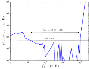
(a) $\widehat{f}_{d}$ vs $f_{d}$ for low SNR

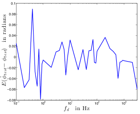
(b) $\widehat{\phi}^{{}^{\prime}}$ vs $f_{d}$ for low SNR

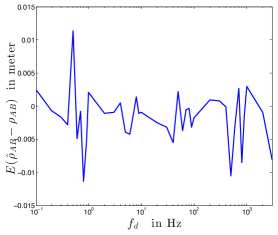
(c) $\widehat{\phi}^{{}^{\prime}}$ vs $f_{d}$ for low SNR

Figure 10: $f_{d}$ estimation error with varying $f_{d}$. Simulated with $\sigma_{j}=1\text{ns}$, $\sigma_{c}=2\text{ns}$. Total duration of simulation is one second with $10^{4}$ Pings per second. Change in $f_{d}$ keeping other parameters of simulation same results in aliasing phenomenon, hence zig-zag fluctuations in simulated results.

V-B2 Eve measuring time difference of arrival of Pings and its subsequent clock edge

As can be seen in Fig.4(a) that Bob can measure the time between periodic arrivals from Alice and the next clock edge of his own clock, $h(1)$. Same measurement $g(1)$ is used by Bob in CLIMEX protocol for delay scaling while responding as proposed while discussing (7). As discussed previously, epoch of such measurements will result in sawtooth. From this it can be concluded that measuring periodic time of arrival with a reference clock would give rise to sawtooth having relative clock parameters of the transmitting and the reference clock. Hence, Eve can measure time of arrival from Alice or Bob with her own clock as a reference clock to estimate $f_{\text{\tiny A}}$ or $f_{\text{\tiny B}}$, assuming she would know her own clock frequency.

However, in CLIMEX protocol the corresponding measurement would be $g(1)$. As can be seen from (6), Eve would need to know $\mathbf{\Delta}$ to make sense of such measurements. Hence, while such measurements would reveal relative clock information in RTT protocol but in CLIMEX protocol such measurements will not be of any use to Eve in absence of knowledge of $\mathbf{\Delta}$.

V-C Shared secret bit generation from exchanged parameters

The parameters estimated between Alice and Bob, $f_{\text{\tiny A}}$, $f_{\text{\tiny B}}$, $\phi_{\text{test}}$ and $\rho_{\text{\tiny AB}}$ are all independent of each other. Alice and Bob generate private keys using these estimated parameters.

V-C1 $\left(f_{\text{\tiny A}},f_{\text{\tiny B}}\right)$

As discussed in section II, clock frequencies of Alice and Bob $\left(f_{\text{\tiny A}},f_{\text{\tiny B}}\right)$ can lie around their nominal frequencies. The deviation around the nominal frequency is usually specified in terms of PPM of the clock. However the nominal frequency of the clock can be variable. Large differences in $f_{\text{\tiny A}}$ and $f_{\text{\tiny B}}$ and hence large values of $|f_{d}|$ will require increased update rate (rate of sending Pings) of the system to sufficiently sample the sawtooth waveform. Smaller values of $|f_{d}|$ would need longer measurement time.

Figure 11: Valid combinations of $\delta f_{\text{\tiny A}}$ and $\delta f_{\text{\tiny B}}$ lie within un-shaded regions. Considering quantization bins of $1$ Hz for $\delta f_{\text{\tiny A}}$ and $\delta f_{\text{\tiny B}}$, total number of combinations are area under the un-shaded region, equals $998^{2}$.

To demonstrate number of possible secret bits from the measurements between Alice and Bob, the experimental setup in [39] is considered with nominal clock frequencies at Alice and Bob, $f_{0}$ of $100$ MHz, update rate of $10^{4}$ Pings per second and clock deviation of $10$ PPM. $f_{\text{\tiny A}}=f_{0}+\delta\!f_{\text{\tiny A}}$, $f_{\text{\tiny B}}=f_{0}+\delta\!f_{\text{\tiny B}}$. Hence, $|f_{d}|=|\delta\!f_{\text{\tiny A}}-\delta\!f_{\text{\tiny B}}|$ and $\delta\!f_{\text{\tiny A}},\delta\!f_{\text{\tiny B}}\sim\mathcal{U}(-500,500)$. However, the accuracy of estimating $\widehat{f}_{d}$ would determine the quantization of range of values of $\delta\!f_{\text{\tiny A}}$ and $\delta\!f_{\text{\tiny B}}$. Figure10 is simulated using above parameters. Where deviation in estimates are recorded for values of $f_{d}$. As can be seen from Fig.10, for large values of $f_{d}$, undersampling of sawtooth results in large errors. While for very low values of $f_{d}$, period of sawtooth waveform is too large to be captured for simulation duration. The non-monotonous, zig-zag nature of curves in simulation results is due to the aliasing effects of waveform sampling while changing the sawtooth frequency.

As shown in Fig.10(a), a limit is set on the performance of the estimator as $E|\widehat{f}_{d}-f_{d}|\leq\Delta f$. This sets frequency quantization bins of size $\Delta f$. Set of possible combinations of $\!f_{\text{\tiny A}}$ and $\!f_{\text{\tiny B}}$ , $\mathcal{T}$, constraining the performance of estimating $f_{d}$ can be written as

$$\mathcal{T}:=$$ (16)

$$\!\!\!\!\!\!\!\!\!\!\!\!\!\!\!\!\!\!\left\{(\delta f_{\text{\tiny A}},\delta f_{\text{\tiny B}}):E|\widehat{f}_{d}-f_{d}|\leq\Delta f,\delta f_{\text{\tiny A}}\ \mbox{and}\ \delta f_{\text{\tiny B}}\in(1,2,..)\right\}.\ \$$

Cardinality of the set $|\mathcal{T}|$ determines number of secret bits extracted from uncertainty in values of $f_{\text{\tiny A}}$ and $f_{\text{\tiny B}}$. As shown in the Fig.10(a), for $\Delta f=0.5$ Hz, possible values of $f_{d}$ lies from $2$ to $1000$ Hz. The number of combinations of $f_{\text{\tiny A}}$ and $f_{\text{\tiny B}}$ pair can be computed as area under the un-shaded regions in Fig.11, when $\delta\!f_{\text{\tiny A}}$ and $\delta\!f_{\text{\tiny B}}$ are quantized by $1$ Hz bins. Area of the un-shaded regions can be computed as sum of areas of the two triangles in the Fig.11, which is $|\mathcal{T}|=998^{2}$. Thus, total number of secret bits extracted from uncertainty of $\left(f_{\text{\tiny A}},f_{\text{\tiny B}}\right)$ combinations is $N_{f}=\log_{2}(|\mathcal{T}|)\sim 20$ bits.

V-C2 $\phi_{\text{test}}$

As can be seen in Fig.10(b), the parameter $\phi_{\text{test}}$ can be resolved with precision of $0.1$ radian for the considered noise and system parameters. So, the number of possible secret bits from uncertainties in estimating $\phi_{\text{test}}$ is, $N_{\phi}=\log_{2}(2\pi/0.1)\sim 6$ bits.

V-C3 $\rho_{\text{\tiny AB}}$

From Fig.10(c), precision of estimating distance between Alice and Bob can be upto $2$ cm. Such a precision in range measurements can be obtained even in present day commercial ranging devices [45]. Thus for a possible range of $100$ meters between Alice and Bob. Number of possible uncertainties and hence number of secret bits are $N_{\rho}=100/0.02\sim 12$ bits.

Thus, total number of possible secret bits considering the system and noise parameters discussed above can be

$$N=N_{f}+N_{\phi}+N_{\rho}\sim 38\,\mbox{bits}.$$ (17)

Above analysis is simplified as the range of parameters and their bins are chosen conservatively. However, it serves the purpose of demonstrating the possibility of extracting secret bits from the CLIMEX protocol.

V-D Eve an active adversary

Figure 12: Eve trying to infiltrate the exchanges between Alice and Bob. Eve’s response can show up as outlier in sawtooth measurement if Eve can not estimate all the distances in the setup besides estimating all clock parameters simultaneously.

Figure 13: Alice and Bob are disconnected, Eve can talk to both and tries to impersonate Bob

Alice and Bob can track the generated sawtooth waveforms from RTT measurements as valid signatures. For Eve to either impersonate or to infiltrate the exchanges without being detected, she has to ensure that the time of arrival of her signal at Alice or Bob should fall on the sawtooth waveform being generated from the measurements. To achieve this, she has to estimate all the distances, $\rho_{\text{\tiny AB}}$, $\rho_{\text{\tiny BE}}$ and $\rho_{\text{\tiny AE}}$ besides estimating all clock parameters for Eve to transmit at the right time so to be able to fit its response on a sawtooth produced at Alice or Bob. Figure 12 illustrates a response called ’False Response’ from Eve attempting to infiltrate message exchange between Alice and Bob but instead showing up as an outlier. It should be noted that Eve has to estimate more parameters than Alice and Bob in order to infiltrate. Additionally, as can be seen from (14), the three distances are non-observable from the measurements between Alice and Bob. So, Eve does not get enough information to infiltrate or impersonate the exchanges between Alice and Bob.

Eve as an active adversary can also try to participate in mutual signal exchanges between Alice and Bob. Particularly in situations when direct communication between Alice and Bob gets blocked without them knowing it, as shown in Fig.13. Here Eve gets an opportunity to impersonate the responding node. In such situations, the sawtooth waveform in the measurement can come again to rescue. As discussed above, Eve will have to transmit at times with precise knowledge of all parameters. Even the sawtooth measurement would provide some robustness to jamming. Resistance against any timing attack through jamming or worm-hole attack can also be resisted while tracking the sawtooth signature in time or arrival of signals [27]. Correlation properties of sawtooth waveform would provide some level of resistance against jamming and similar attacks.

V-E Non-observable parameters

Clock frequencies of Alice and Bob, $f_{\text{\tiny A}}$, $f_{\text{\tiny B}}$ are non-observable to Eve from measurements. As can be seen from the following arguments.

1. It is assumed that Alice and Bob know their own clock frequencies $f_{\text{\tiny A}}$ and $f_{\text{\tiny B}}$.

2. Alice can estimate $f_{d}$ (8) and Alice can also trivially estimate Bob’s clock frequency $f_{\text{\tiny B}}=f_{d}-f_{\text{\tiny A}}$, (11).

3. Similarly, Bob can estimate its own and Alice’s frequencies.

4. It can be seen from (4), (5) and (6) that $f_{\text{\tiny A}}$ and $f_{\text{\tiny B}}$, individual clock frequencies of Alice and Bob are non-observable these RTT measurements. This is true even without using any random transmit delay $\mathbf{\Delta}$. It is assumed that no one else knows Alice’s and Bob’s clock frequencies. In case of Alice and Bob not revealing it by themselves, it will require direct physical access to Alice’s and Bob’s clock to measure their frequencies.

5. As discussed in previous sections, Alice and Bob can estimate $f_{\text{\tiny A}}$ and $f_{\text{\tiny B}}$. However, these frequencies are non-observable to Eve or anyone else.

6. Usage of $\mathbf{\Delta}$ for deliberate dithering of measurements further makes it difficult for Eve to eavesdrop.

Mathematically, it should be observed from (4), (5) and (6), in RTT measurements collected from CLIMEX protocol, $f_{\text{\tiny A}}$ and $f_{\text{\tiny B}}$ are non-observable and can not be estimated unless $f_{\text{\tiny A}}$ or $f_{\text{\tiny B}}$ is known. It means that Eve can not estimate these parameters from any possible measurements when Alice and Bob follow the CLIMEX protocol.

VI Discussions

The idea presented in this paper is conceived from the testbed outcome. Clock parameters and distances are physical parameter which can be controlled and can be setup to a good extent based on necessity. Different parameters for generating secret bits discussed above have different properties and relevance in the scheme. While frequencies and the distance have unknown values in the system which can be setup by the users in the system to certain precision, the phase is usually out of control of the users. Frequency of the clock and position of Alice or Bob can possibly be obtained by Eve by some other physical access or means. But instantaneous relative phase of two clocks separated by a distance can only be obtained at the time of operation. As discussed in previous section, the parameter $\phi_{\text{test}}$ amounts to nearly $6$ shared secret bits in the considered setup, it is more infeasible to be revealed to the adversary.

In present day consumer electronic systems, range of parameters chosen in previous section to derive number of bits can be larger. Update rate can be possibly many orders higher. Distance estimation with sufficient accuracy is possible of up to a kilo-meter. Clock frequency of nodes can be in hundreds of mega-hertz. Overall, higher number of shared secret bits is possible with aggressive selection of system parameters. Number of shared secret bits can also be increased by successive execution of CLIMEX protocol.

Considering scope of future work, the proposed CLIMEX protocol can also be applied for following general application scenarios

1. Secure ranging and secure positioning in scenarios such as [27, 31, 46, 47].

2. Time synchronization in wireless networks can be secured with the CLIMEX implementation between nodes. While achieving the time synchronization at the same time in schemes such as [48].

VII Conclusion

CLIMEX as a secure wireless protocol is proposed for establishing secret bits between Alice and Bob, based on a round-trip-scheme where Alice and Bob sequentially set up the information exchange in a ping-response fashion. A CLIMEX ping by Alice is securitized by an inherent synthetic clock edge or time-domain dithering, only known to Alice. The subsequent response by Bob is securitized by an amplitude-domain scaling. At Alice, a double-modulus nonlinear measurement model provides means for extracting the inherent physical parameters of both Alice and Bob, based on repeated measurements of Bob responses, and the unique knowledge of Alice’s own inherent physical parameters. The physical parameters of Alice and Bob form the foundation for the secret bits. Subsequently, for reciprocity Bob is taking Eve’s role, and vice versa. By CLIMEX protocol, Bob is retrieving the secret bits, mutatis mutandis. For a passive adversary Eve with at least the same capabilities as Alice and Bob, it is shown that the physical parameters are unobservable. In addition, for an active impersonator Eve it is shown that its actions are detectable at Alice and Bob, manifested as outlier measurements. Use of IEEE 802.15.4a like impulse radio UWB technology is considered for CLIMEX implementation. In-house testbed based on Xilinx Virtex-5 and ACAM time-to-digital-converters for required sub-clock resolution provided us with supporting experimental data and design parameters, showing potential for some 38 possible secret bits in typical use cases. Potential of CLIMEX can be foreseen for use cases with short to medium range distances (1-100 meters) between the nodes, including a variety of services for wireless communications, ranging and positioning.

References

- [1] R. H. Weber, “Internet of things – new security and privacy challenges,” Computer Law & Security Review, vol. 26, no. 1, pp. 23 – 30, 2010. [Online]. Available: http://www.sciencedirect.com/science/article/pii/S0267364909001939
- [2] Q. Jing, A. V. Vasilakos, J. Wan, J. Lu, and D. Qiu, “Security of the internet of things: perspectives and challenges,” Wireless Networks, vol. 20, no. 8, pp. 2481–2501, 2014.
- [3] A. Mukherjee, “Physical-layer security in the internet of things: Sensing and communication confidentiality under resource constraints,” Proceedings of the IEEE, vol. 103, no. 10, pp. 1747–1761, Oct 2015.
- [4] W. Trappe, “The challenges facing physical layer security,” Communications Magazine, IEEE, vol. 53, no. 6, pp. 16–20, June 2015.
- [5] K. D. Kim and P. R. Kumar, “Cyber physical systems: A perspective at the centennial,” Proceedings of the IEEE, vol. 100, no. Special Centennial Issue, pp. 1287–1308, May 2012.
- [6] K. Ren, H. Su, and Q. Wang, “Secret key generation exploiting channel characteristics in wireless communications,” IEEE Wireless Communications, vol. 18, no. 4, pp. 6–12, August 2011.
- [7] M. Bloch and J. Barros, Physical-layer security: from information theory to security engineering. Cambridge University Press, 2011.
- [8] E. Jorswieck, S. Tomasin, and A. Sezgin, “Broadcasting into the uncertainty: Authentication and confidentiality by physical-layer processing,” Proceedings of the IEEE, vol. 103, no. 10, pp. 1702–1724, Oct 2015.
- [9] K. Zeng, “Physical layer key generation in wireless networks: challenges and opportunities,” Communications Magazine, IEEE, vol. 53, no. 6, pp. 33–39, June 2015.
- [10] J. Zhang, T. Q. Duong, A. Marshall, and R. Woods, “Key generation from wireless channels: A review,” IEEE Access, vol. 4, pp. 614–626, 2016.
- [11] A. Mukherjee, S. A. A. Fakoorian, J. Huang, and A. L. Swindlehurst, “Principles of physical layer security in multiuser wireless networks: A survey,” IEEE Communications Surveys Tutorials, vol. 16, no. 3, pp. 1550–1573, Third 2014.
- [12] L. Xiao, L. Greenstein, N. B. Mandayam, and W. Trappe, “Using the physical layer for wireless authentication in time-variant channels,” Wireless Communications, IEEE Transactions on, vol. 7, no. 7, pp. 2571–2579, July 2008.
- [13] K. Zeng, K. Govindan, and P. Mohapatra, “Non-cryptographic authentication and identification in wireless networks,” network security, vol. 1, p. 3, 2010.
- [14] Q. Xu, R. Zheng, W. Saad, and Z. Han, “Device fingerprinting in wireless networks: Challenges and opportunities,” IEEE Communications Surveys Tutorials, vol. 18, no. 1, pp. 94–104, Firstquarter 2016.
- [15] S. Jana, S. N. Premnath, M. Clark, S. K. Kasera, N. Patwari, and S. V. Krishnamurthy, “On the effectiveness of secret key extraction from wireless signal strength in real environments,” in Proceedings of the 15th Annual International Conference on Mobile Computing and Networking, ser. MobiCom ’09. New York, NY, USA: ACM, 2009, pp. 321–332. [Online]. Available: http://doi.acm.org/10.1145/1614320.1614356
- [16] M. M. U. Rahman, A. Yasmeen, and J. Gross, “Phy layer authentication via drifting oscillators,” in 2014 IEEE Global Communications Conference, Dec 2014, pp. 716–721.
- [17] H. Takesue, S. W. Nam, Q. Zhang, R. H. Hadfield, T. Honjo, K. Tamaki, and Y. Yamamoto, “Quantum key distribution over a 40-db channel loss using superconducting single-photon detectors,” Nature photonics, vol. 1, no. 6, pp. 343–348, 2007.
- [18] P. Papadimitratos, M. Poturalski, P. Schaller, P. Lafourcade, D. Basin, S. Capkun, and J. P. Hubaux, “Secure neighborhood discovery: a fundamental element for mobile ad hoc networking,” IEEE Communications Magazine, vol. 46, no. 2, pp. 132–139, February 2008.
- [19] V. Brik, S. Banerjee, M. Gruteser, and S. Oh, “Wireless device identification with radiometric signatures,” in Proceedings of the 14th ACM International Conference on Mobile Computing and Networking, ser. MobiCom ’08. New York, NY, USA: ACM, 2008, pp. 116–127. [Online]. Available: http://doi.acm.org/10.1145/1409944.1409959
- [20] W. Hou, X. Wang, J. Y. Chouinard, and A. Refaey, “Physical layer authentication for mobile systems with time-varying carrier frequency offsets,” IEEE Transactions on Communications, vol. 62, no. 5, pp. 1658–1667, May 2014.
- [21] S. Jana and S. K. Kasera, “On fast and accurate detection of unauthorized wireless access points using clock skews,” IEEE Transactions on Mobile Computing, vol. 9, no. 3, pp. 449–462, March 2010.
- [22] Y. Shi and M. A. Jensen, “Improved radiometric identification of wireless devices using MIMO transmission,” IEEE Transactions on Information Forensics and Security, vol. 6, no. 4, pp. 1346–1354, Dec 2011.
- [23] K. Sun, P. Ning, and C. Wang, “Secure and resilient clock synchronization in wireless sensor networks,” IEEE Journal on Selected Areas in Communications, vol. 24, no. 2, pp. 395–408, Feb 2006.
- [24] A. Treytl, G. Gaderer, B. Hirschler, and R. Cohen, “Traps and pitfalls in secure clock synchronization,” in 2007 IEEE International Symposium on Precision Clock Synchronization for Measurement, Control and Communication, Oct 2007, pp. 18–24.
- [25] J. T. Chiang, J. J. Haas, Y. C. Hu, P. R. Kumar, and J. Choi, “Fundamental limits on secure clock synchronization and man-in-the-middle detection in fixed wireless networks,” in IEEE INFOCOM 2009, April 2009, pp. 1962–1970.
- [26] B. Kailkhura, V. S. S. Nadendla, and P. K. Varshney, “Distributed inference in the presence of eavesdroppers: a survey,” IEEE Communications Magazine, vol. 53, no. 6, pp. 40–46, June 2015.
- [27] S. Capkun and J.-P. Hubaux, “Secure positioning in wireless networks,” Selected Areas in Communications, IEEE Journal on, vol. 24, no. 2, pp. 221–232, Feb 2006.
- [28] K. B. Rasmussen and S. Capkun, “Realization of RF distance bounding.” in USENIX Security Symposium, 2010, pp. 389–402.
- [29] S. Brands and D. Chaum, Advances in Cryptology — EUROCRYPT ’93: Workshop on the Theory and Application of Cryptographic Techniques Lofthus, Norway, May 23–27, 1993 Proceedings. Berlin, Heidelberg: Springer Berlin Heidelberg, 1994, ch. Distance-Bounding Protocols, pp. 344–359. [Online]. Available: http://dx.doi.org/10.1007/3-540-48285-7_30
- [30] S. Salimi and P. Papadimitratos, “Pairwise secret key agreement based on location-derived common randomness,” in International Zurich Seminar on Communications, 2016.
- [31] P. Papadimitratos, L. Buttyan, T. Holczer, E. Schoch, J. Freudiger, M. Raya, Z. Ma, F. Kargl, A. Kung, and J. P. Hubaux, “Secure vehicular communication systems: design and architecture,” IEEE Communications Magazine, vol. 46, no. 11, pp. 100–109, November 2008.
- [32] N. O. Tippenhauer, H. Luecken, M. Kuhn, and S. Capkun, “UWB rapid-bit-exchange system for distance bounding,” in Proceedings of the 8th ACM Conference on Security & Privacy in Wireless and Mobile Networks. ACM, 2015, p. 2.
- [33] C. Neuberg, P. Papadimitratos, C. Fragouli, and R. Urbanke, “A mobile world of security-the model,” in Information Sciences and Systems (CISS), 2011 45th Annual Conference on. IEEE, 2011, pp. 1–6.
- [34] M. Zafer, D. Agrawal, and M. Srivatsa, “Limitations of generating a secret key using wireless fading under active adversary,” IEEE/ACM Transactions on Networking, vol. 20, no. 5, pp. 1440–1451, Oct 2012.
- [35] R. Liu and W. Trappe, Securing wireless communications at the physical layer. Springer, 2010, vol. 7.
- [36] P. Papadimitratos, V. Gligor, and J.-P. Hubaux, “Securing vehicular communications-assumptions, requirements, and principles,” in Workshop on Embedded Security in Cars (ESCAR), no. LCA-CONF-2006-021, 2006, pp. 5–14.
- [37] S. Mathur, A. Reznik, C. Ye, R. Mukherjee, A. Rahman, Y. Shah, W. Trappe, and N. Mandayam, “Exploiting the physical layer for enhanced security [security and privacy in emerging wireless networks],” IEEE Wireless Communications, vol. 17, no. 5, pp. 63–70, October 2010.
- [38] A. De Angelis, S. Dwivedi, and P. Händel, “Characterization of a flexible UWB sensor for indoor localization,” Instrumentation and Measurement, IEEE Transactions on, vol. 62, no. 5, pp. 905–913, May 2013.
- [39] S. Dwivedi, A. De Angelis, D. Zachariah, and P. Händel, “Joint ranging and clock parameter estimation by wireless round trip time measurements,” Selected Areas in Communications, IEEE Journal on, vol. 33, no. 11, pp. 2379–2390, Nov 2015.
- [40] “ACAM messelectronic gmbh: TDC - time-to-digital converters,” http://www.acam.de/download-center/tdc/, 2017, [online; accessed 20-March-2017].
-
[41]
“Texas instruments TDC7200,”
http://www.ti.com/lit/ds/symlink/tdc7200.pdf, 2017, [online; accessed 20-March-2017]. -
[42]
“Precision time protocol (PTP),”
https://en.wikipedia.org/wiki/Precision_Time_Protocol, 2017, [online; accessed 20-March-2017]. - [43] J. Han and D. k. Jeong, “Practical considerations in the design and implementation of time synchronization systems using IEEE 1588,” IEEE Communications Magazine, vol. 47, no. 11, pp. 164–170, November 2009.
- [44] S. M. Kay, Fundamentals of statistical signal processing, volume I: estimation theory. Prentice Hall, 1993.
- [45] “Decawave ranging radios,” http://www.decawave.com/, 2017, [online; accessed 20-March-2017].
- [46] S. Dwivedi, D. Zachariah, A. De Angelis, and P. Handel, “Cooperative decentralized localization using scheduled wireless transmissions,” Communications Letters, IEEE, vol. 17, no. 6, pp. 1240–1243, June 2013.
- [47] G. R. de Campos, P. Falcone, R. Hult, H. Wymeersch, and J. Sjöberg, “Traffic coordination at road intersections: Autonomous decision-making algorithms using model-based heuristics,” IEEE Intelligent Transportation Systems Magazine, vol. 9, no. 1, pp. 8–21, Spring 2017.
- [48] D. Zachariah, S. Dwivedi, P. Händel, and P. Stoica, “Scalable and passive wireless network clock synchronization in los environments,” IEEE Transactions on Wireless Communications, vol. 16, no. 6, pp. 3536–3546, June 2017.