Independent Low-Rank Matrix Analysis Based on Complex Student’s $t$-Distribution for Blind Audio Source Separation

Abstract

In this paper, we generalize a source generative model in a state-of-the-art blind source separation (BSS), independent low-rank matrix analysis (ILRMA). ILRMA is a unified method of frequency-domain independent component analysis and nonnegative matrix factorization and can provide better performance for audio BSS tasks. To further improve the performance and stability of the separation, we introduce an isotropic complex Student’s $t$-distribution as a source generative model, which includes the isotropic complex Gaussian distribution used in conventional ILRMA. Experiments are conducted using both music and speech BSS tasks, and the results show the validity of the proposed method.

Index Terms—  Blind source separation, nonnegative matrix factorization, independent component analysis, Student’s $t$-distribution, generative model

1 Introduction

Blind source separation (BSS) is a technique for extracting specific sources from an observed multichannel mixture signal without knowing a priori information about the mixing system. The most popular algorithm for BSS is called independent component analysis (ICA) [1], which assumes statistical independence between the sources and estimates the demixing system. In particular, BSS for audio signals has been well studied. For a mixture of audio signals, since the sources are convolved owing to the room reverberation, ICA is often applied to the time-frequency domain signal, which is called the spectrogram obtained by a short-time Fourier transform (STFT). Frequency-domain ICA (FDICA) [2, 3] independently applies ICA to the time-series signals in each frequency, then the permutation of the estimated signals is aligned on the basis of several criteria. As an elegant solution of this permutation alignment problem, independent vector analysis (IVA) [4] was proposed, which assumes higher-order dependences among the frequency components in each source, thus avoiding the permutation problem. In [5], fast and stable optimization of IVA (AuxIVA) was derived using an auxiliary function technique that is also known as a majorization-minimization (MM) algorithm [6].

As another means of audio source separation, nonnegative matrix factorization (NMF) [7] has been a very popular approach during the last decade. NMF is a parts-based decomposition (low-rank approximation) of a nonnegative data matrix, which is typically a power or amplitude spectrogram, and the significant parts (bases and activations) can be used for source separation. Also, NMF can be statistically interpreted as a parameter estimation based on a generative model of data, and the distribution of the model defines a cost function (divergence) in NMF. For example, it was revealed that NMF based on Itakura–Saito divergence (ISNMF) assumes an isotropic complex Gaussian distribution independently defined in each time-frequency slot [8]. Recently, a new NMF based on an isotropic complex Cauchy distribution (Cauchy NMF) [9] and its generalization, NMF based on a complex Student’s $t$-distribution ($t$-NMF) [10], have been proposed. $t$-NMF includes both ISNMF and Cauchy NMF as special cases, and it has been reported that $t$-NMF provides better and more stable source separation for simple audio signals [10].

For multichannel audio source separation, NMF has been extended to multichannel NMF (MNMF) [11, 12, 13]. MNMF employs a sourcewise spatial parameter, spatial covariance, that approximates the mixing system to achieve source separation. However, the separation performance of MNMF strongly depends on the initialization of the parameters because of the difficulty of the optimization. This problem was addressed by exploiting a complex Student’s $t$-distribution as a source generative model in MNMF ($t$-MNMF) [14], which may lead to initialization-robust optimization.

NMF has been unified with the conventional ICA- or IVA-based techniques, which allows us to simultaneously model the sourcewise time-frequency structure and the statistical independence between sources. This state-of-the-art BSS is called independent low-rank matrix analysis (ILRMA) [15, 16], which is a natural extension of IVA from a vector to a low-rank matrix source model. ILRMA is equivalent to a special case of MNMF; ILRMA assumes that the mixing system is invertible and estimates the demixing system similarly to FDICA or IVA, whereas MNMF estimates the mixing system (spatial covariance) required for separation. For the optimization problem, ILRMA is much faster and more stable than MNMF. In this paper, we generalize the source generative model in ILRMA from the complex Gaussian distribution to the complex Student’s $t$-distribution, which is expected to further improve the performance and stability of the parameter initialization. The relationship among the conventional methods and the proposed ILRMA is depicted in Fig. 1. As shown in this figure, the proposed ILRMA can be referred to as a new extension of conventional ILRMA as well as a computationally efficient solution for the dual problem of $t$-MNMF under a spatially rank-1 condition.

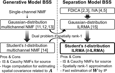
Fig. 1: Relation among conventional methods and proposed ILRMA.

2 Conventional methods

2.1 Formulation

Let $N$ and $M$ be the numbers of sources and channels, respectively. The complex-valued source, observed, and estimated signals are defined as $\bm{s}_{ij}\!=\!(s_{ij,1},\cdots,s_{ij,N})^{\rm T}$, $\bm{x}_{ij}\!=\!(x_{ij,1},\cdots,x_{ij,M})^{\rm T}$, and $\bm{y}_{ij}\!=\!(y_{ij,1},\cdots,y_{ij,N})^{\rm T}$, where $i\!=\!1,\cdots,I$; $j\!=\!1,\cdots,J$; $n\!=\!1,\cdots,N$; and $m\!=\!1,\cdots,M$ are the integral indexes of the frequency bins, time frames, sources, and channels, respectively, and ^T denotes a transpose. We also denote the spectrograms of the source, observed, and estimated signals as $\bm{S}_{n}\ {\in\mathbb{C}^{\scalebox{0.6}{$I{\times}J$}}}$, $\bm{X}_{m}\ {\in\mathbb{C}^{\scalebox{0.6}{$I{\times}J$}}}$, and $\bm{Y}_{n}\ {\in\mathbb{C}^{\scalebox{0.6}{$I{\times}J$}}}$, whose elements are $s_{ij,n}$, $x_{ij,m}$, and $y_{ij,n}$, respectively. In FDICA, IVA, and ILRMA, the following mixing system is assumed:

$$\bm{x}_{ij}=\bm{A}_{i}\bm{s}_{ij},$$ (1)

where $\bm{A}_{i}\!=\!(\bm{a}_{i,1}~{}\cdots~{}\bm{a}_{i,N})\ {\in\mathbb{C}^{\scalebox{0.6}{$M{\times}N$}}}$ is a frequency-wise mixing matrix and $\bm{a}_{i,n}$ is the steering vector for the $n$th source. The assumption of the mixing system (1) corresponds to restricting the spatial covariance in MNMF to a rank-1 matrix [15]. The estimated signal $\bm{y}_{ij}$ can be obtained by assuming $M\!=\!N$ and estimating the frequency-wise demixing matrix $\bm{W}_{i}\!=\!(\bm{w}_{i,1}~{}\cdots~{}\bm{w}_{i,N})^{\rm H}\!=\!\bm{A}_{i}^{-1}$ as

$$\bm{y}_{ij}=\bm{W}_{i}\bm{x}_{ij},$$ (2)

where $\bm{w}_{i,n}$ is the demixing filter for the $n$th source and ^H denotes a Hermitian transpose. FDICA, IVA, and ILRMA estimate both $\bm{W}_{i}$ and $\bm{y}_{ij}$ from only the observation $\bm{x}_{ij}$ assuming statistical independence between $s_{ij,n}$ and $s_{ij,n^{\prime}}$, where $n^{\prime}\!\neq\!n$.

2.2 ILRMA

ILRMA assumes the following time-varying distribution as the generative model of each source:

$$\prod_{i,j}p(y_{ij,n})= \ \prod_{i,j}\frac{1}{\pi r_{ij,n}}\exp\left(-\frac{|y_{ij,n}|^{2}}{r_{ij,n}}\right),$$ (3)

$$r_{ij,n}= \ \sum_{l}t_{il,n}v_{lj,n},$$ (4)

where the local distribution $p(y_{ij,n})$ is defined as a circularly symmetric (isotropic) complex Gaussian distribution, i.e., the probability of $p(y_{ij,n})$ only depends on the power of the complex value $y_{ij,n}$. Also, $r_{ij,n}$ is a time-frequency-varying nonnegative variance and corresponds to the expectation of the power of $y_{ij,n}$, i.e., $r_{ij,n}\!=\!{\rm E}[|y_{ij,n}|^{2}]$. This is because $p(y_{ij,n})$ is isotropic in the complex plane. Moreover, $t_{il,n}$ and $v_{lj,n}$ are the NMF parameters called basis and activation, respectively, $l\!=\!1,\cdots,L$ is the integral index, and $L$ is set to a much smaller value than $\min{(I,J)}$, which leads to the low-rank approximation. Since the variance $r_{ij,n}$ can fluctuate depending on the time frame, (3) becomes a non-Gaussian distribution. The negative log-likelihood function ${\cal L}$ based on (3) can be obtained as follows by assuming independence between each source and each time frame:

$${\cal L}={\rm const.}-2J\sum_{i}\log|\det\bm{W}_{i}|+\sum_{i,j,n}\left(\log{r_{ij,n}}+\frac{|y_{ij,n}|^{2}}{r_{ij,n}}\right).$$ (5)

Regarding the estimation of $t_{il,n}$ and $v_{lj,n}$, the minimization of (5) is equivalent to the optimization in ISNMF that minimizes the Itakura–Saito divergence between $|\bm{Y}_{n}|^{.2}$ and $\bm{T}_{n}\bm{V}_{n}$, where $\bm{T}_{n}\ {\in\mathbb{R}_{\scalebox{0.6}{$\geq 0$}}^{\scalebox{0.6}{$I{\times}L$}}}$ and $\bm{V}_{n}\ {\in\mathbb{R}_{\scalebox{0.6}{$\geq 0$}}^{\scalebox{0.6}{$L{\times}J$}}}$ are the basis and activation matrices whose elements are $t_{il,n}$ and $v_{lj,n}$, and the absolute value and the dotted exponent for a matrix denote an element-wise absolute value and exponent, respectively.

Fig. 2 shows the conceptual model of ILRMA. When the original sources have a low-rank spectrogram $|\bm{S}_{n}|^{.2}$, the spectrogram of their mixture, $|\bm{X}_{m}|^{.2}$, should be more complicated, where the rank of $|\bm{X}_{m}|^{.2}$ will be greater than that of $|\bm{S}_{n}|^{.2}$. On the basis of this assumption, in ILRMA, the low-rank constraint for each estimated spectrogram $|\bm{Y}_{n}|^{.2}$ is introduced by employing NMF. The demixing matrix $\bm{W}_{i}$ is estimated so that the spectrogram of the estimated signal $|\bm{Y}_{n}|^{.2}$ becomes a low-rank matrix modeled by $\bm{T}_{n}\bm{V}_{n}$, whose rank is at most $L$. The estimation of $\bm{W}_{i}$, $\bm{T}_{n}$, and $\bm{V}_{n}$ can consistently be carried out by minimizing (5) in a fully blind manner. Note that ILRMA is theoretically equivalent to conventional MNMF only when the rank-1 spatial model is assumed, which yields a stable and computationally efficient algorithm for ILRMA. This issue and the convergence-guaranteed fast update rules for $\bm{W}_{i}$, $\bm{T}_{n}$, and $\bm{V}_{n}$ can be found in [15].

2.3 NMF and MNMF based on complex Student’s $t$-distribution

As revealed in [8], ISNMF justifies the additivity of power spectra in the expectation sense using the stable property of a complex Gaussian distribution. Regarding the amplitude spectrogram, Cauchy NMF [9] can be considered as a counterpart of ISNMF; the additivity of amplitude spectra is justified using the stable property of a complex Cauchy distribution. In [10], these theoretically justified NMFs were generalized by employing a complex Student’s $t$-distribution, which includes the complex Gaussian and complex Cauchy distributions as special cases when the degree-of-freedom parameter $\nu\!>\!0$ is set to $\nu\!\rightarrow\!\infty$ and $\nu\!=\!1$, respectively. Although complex Student $t$-distributions with other values of $\nu$ do not have the stable property, $t$-NMF provides better and more robust source separation for simple audio signals when $\nu$ is approximately two. Also, the generalization of MNMF with a complex Student’s $t$-distribution was proposed [14] with the aim of improving the robustness of the parameter initialization.

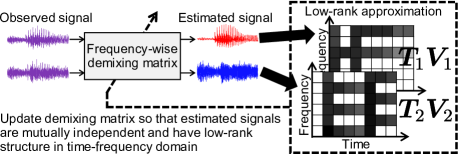
Fig. 2: Conceptual model of ILRMA.

3 Proposed method

3.1 ILRMA based on complex Student’s $t$-distribution

Motivated by the improvements in $t$-NMF, we propose the introduction of a complex Student’s $t$-distribution as a source generative model in ILRMA ($t$-ILRMA), which is a generalization of conventional Gaussian ILRMA based on (3). The generative model in $t$-ILRMA is as follows:

$$\prod_{i,j}p(y_{ij,n})= \ \prod_{i,j}\frac{1}{\pi\sigma_{ij,n}^{2}}\left(1+\frac{2}{\nu}\frac{|y_{ijn}|^{2}}{\sigma_{ij,n}^{2}}\right)^{-\frac{2+\nu}{2}},$$ (6)

$$\sigma_{ij,n}^{p}= \ \sum_{l}t_{il,n}v_{lj,n},$$ (7)

where the local distribution $p(y_{ij,n})$ is defined as an isotropic complex Student’s $t$-distribution, $\sigma_{ij,n}$ is a time-frequency-varying nonnegative scale and corresponds to an amplitude spectrum $|y_{ij,n}|$, and $p$ is a parameter that defines the domain of the NMF model $\bm{T}_{n}\bm{V}_{n}$ and should satisfy $1\!\leq\!p\!\leq\!2$. When $\nu\!\rightarrow\!\infty$ and $p\!=\!2$, (6) corresponds to the generative model in ISNMF, and when $\nu\!=\!1$ and $p\!=\!1$, (6) corresponds to the generative model in Cauchy NMF. The negative log-likelihood function based on (6) can be obtained as follows by assuming independence between each source and each time frame:

$${\cal L}_{t}= \ {\rm const.}-2J\sum_{i}\log|\det\bm{W}_{i}|$$

$$\ +\sum_{i,j,n}\left[\left(1+\frac{\nu}{2}\right)\log{\left(1+\frac{2}{\nu}\frac{|y_{ij,n}|^{2}}{\sigma_{ij,n}^{2}}\right)}+2\log\sigma_{ij,n}\right].$$ (8)

When $\nu\!\rightarrow\!\infty$ and $p\!=\!2$, (8) coincides with (5).

3.2 Derivation of update rules for demixing matrix

Similar to the derivation described in [15], we apply an MM algorithm and iterative projection (IP) [5] to derive the update rules for the demixing matrix $\bm{W}_{i}$ with a full guarantee of the monotonic convergence. IP was the method originally used to solve the simultaneous vector equations in AuxIVA, which are equivalent to the HEAD problem [17]. Unlike the conventional MNMF methods such as that in [14] that estimate the mixing model $\bm{A}_{i}$ (not the demixing matrix $\bm{W}_{i}$), IP can lead to much faster and more stable estimation of $\bm{W}_{i}$ in BSS, as reported in [15, 5]. However, the major drawback of IP is the limited number of applicable functions; i.e., generally the term $|y_{ij,n}|^{2}\!=\!|\bm{w}_{i,n}^{\rm H}\bm{x}_{ij}|^{2}$ should appear as is in the objective function, e.g., in (5) (should not appear as a part of variable inside a nonlinear function).

For the $t$-ILRMA’s cost function (8), whose $|y_{ij,n}|^{2}$ term is intrinsic, as a trick to enable the introduction of IP, we apply a tangent line inequality to the logarithm terms in (8). The tangent line inequality can be represented as

$$\log\left(\sum_{q}z_{q}\right)\leq\frac{1}{\lambda}\left(\sum_{q}z_{q}-\lambda\right)+\log\lambda,$$ (9)

where $z_{q}$ is the original variable and $\lambda\!>\!0$ is an auxiliary variable. The equality of (9) holds if and only if $\lambda\!=\!\sum_{q}z_{q}$. By applying (9) to the second and third logarithm terms in (8), the following majorization function can be designed:

$${\cal L}_{t}\leq \ {\rm const.}-2J\sum_{i}\log|\det\bm{W}_{i}|$$

$$\ +\sum_{i,j,n}\left[\left(1+\frac{\nu}{2}\right)\frac{1}{\alpha_{ij,n}}\left(1+\frac{2}{\nu}\frac{|y_{ij,n}|^{2}}{\sigma_{ij,n}^{2}}-\alpha_{ij,n}\right)\right.$$

$$\ +\left(1+\frac{\nu}{2}\right)\log\alpha_{ij,n}+\frac{2}{p\beta_{ij,n}}\left(\sum_{l}t_{il,n}v_{lj,n}-\beta_{ij,n}\right)$$

$$\ +\left.\frac{2}{p}\log\beta_{ij,n}\right]$$

$$\equiv \ {\cal L}_{t}^{+},$$ (10)

where $\sigma_{ij,n}\!=\!(\sum_{l}t_{il,n}v_{lj,n})^{1/p}$ is partly substituted, $\alpha_{ij,n},\beta_{ij,n}\!>\!0$ are auxiliary variables, and ${\cal L}_{t}$ and ${\cal L}_{t}^{+}$ become equal only when

$$\alpha_{ij,n}= \ 1+\frac{2}{\nu}\frac{|y_{ij,n}|^{2}}{\sigma_{ij,n}^{2}},$$ (11)

$$\beta_{ij,n}= \ \sum_{l}t_{il,n}v_{lj,n}.$$ (12)

Because $|y_{ij,n}|^{2}\!=\!|\bm{w}_{i,n}^{\rm H}\bm{x}_{ij}|^{2}$ in (10) exists outside the logarithm function, we can apply IP in analogy with the derivation in conventional ILRMA using (5). The majorization function (10) can be reformulated as

$${\cal L}_{t}^{+}= \ {\rm const.}-2J\sum_{i}\log|\det\bm{W}_{i}|+J\sum_{i,n}\bm{w}_{i,n}^{\rm H}\bm{U}_{i,n}\bm{w}_{i,n}$$

$$\ +\sum_{i,j,n}\left[\left(1+\frac{\nu}{2}\right)\left(\alpha_{ij,n}^{-1}-1+\log\alpha_{ij,n}\right)\right.$$

$$\ \left.+\frac{2}{p\beta_{ij,n}}\left(\sum_{l}t_{il,n}v_{lj,n}-\beta_{ij,n}\right)+\frac{2}{p}\log\beta_{ij,n}\right],$$ (13)

$$\bm{U}_{i,n}= \ \frac{1}{J}\left(\frac{2}{\nu}+1\right)\sum_{j}\frac{1}{\alpha_{ij,n}\sigma_{ij,n}^{2}}\bm{x}_{ij}\bm{x}_{ij}^{\rm H}.$$ (14)

Since the majorization function (13) is the same form as that of AuxIVA with respect to $\bm{w}_{i,n}$, the following simultaneous equations are obtained:

$$\bm{w}_{i,k}^{\rm H}\bm{U}_{i,n}\bm{w}_{i,n}=\delta_{kn},$$ (15)

where $\delta_{kn}\!=\!1$ when $k\!=\!n$ and $\delta_{kn}\!=\!0$ when $k\!\neq\!n$. By applying IP to (15), we can obtain the update rules for the demixing matrix as

$$\bm{w}_{i,n}\leftarrow \ \left(\bm{W}_{i}\bm{U}_{i,n}\right)^{-1}\bm{e}_{n},$$ (16)

$$\bm{w}_{i,n}\leftarrow \ \frac{\bm{w}_{i,n}}{\sqrt{\bm{w}_{i,n}^{\rm H}\bm{U}_{i,n}\bm{w}_{i,n}}},$$ (17)

where $\bm{e}_{n}$ denotes the unit vector with the $n$th element equal to unity. After the update of $\bm{W}_{i}$, the separated signal $\bm{y}_{ij}$ should be updated as $y_{ij,n}\!\leftarrow\!\bm{w}_{ij,n}^{\rm H}\bm{x}_{ij}$.

3.3 Derivation of update rules for NMF parameters

The update rules for $t_{il,n}$ and $v_{lj,n}$ can be derived by the MM algorithm, which is a popular approach for NMF. To obtain the differentiable majorization function for NMF parameters in (10), we apply Jensen’s inequality to $\sigma_{ij,n}^{-2}=(\sum_{l}t_{il,n}v_{lj,n})^{-2/p}$. Jensen’s inequality can be represented as

$$\left(\sum_{q}z_{q}\right)^{-2/p}=\left(\sum_{q}\mu_{q}\frac{z_{q}}{\mu_{q}}\right)^{-2/p}\leq\sum_{q}\mu_{q}\left(\frac{z_{q}}{\mu_{q}}\right)^{-2/p}=\sum_{q}\mu_{q}^{\frac{2}{p}+1}z_{q}^{-\frac{2}{p}},$$ (18)

where $\mu_{q}\!>\!0$ is an auxiliary variable that satisfies $\sum_{q}\mu_{q}\!=\!1$. Note that the left-hand side of (18) is a convex function for the variable $z_{q}$ because we consider $1\!\leq\!p\!\leq\!2$. The equality of (18) holds if and only if $\mu_{q}\!=\!z_{q}/\sum_{q^{\prime}}z_{q^{\prime}}$. By applying (18) to $\sigma_{ij,n}^{-2}\!=\!(\sum_{l}t_{il,n}v_{lj,n})^{-2/p}$ in (8), the following majorization function can be designed:

$${\cal L}_{t}^{+}\leq \ {\rm const.}-2J\sum_{i}\log|\det\bm{W}_{i}|$$

$$+\!\sum_{i,j,n}\left[\left(1+\frac{\nu}{2}\right)\frac{1}{\alpha_{ij,n}}\left(1+\frac{2}{\nu}|y_{ij,n}|^{2}\!\sum_{l}\gamma_{ij,nl}^{\frac{2}{p}+1}t_{il,n}^{-\frac{2}{p}}v_{lj,n}^{-\frac{2}{p}}-\alpha_{ij,n}\right)\right.$$

$$+\left(1+\frac{\nu}{2}\right)\log\alpha_{ij,n}+\frac{2}{p\beta_{ij,n}}\left(\sum_{l}t_{il,n}v_{lj,n}-\beta_{ij,n}\right)$$

$$+\left.\frac{2}{p}\log\beta_{ij,n}\right]$$

$$\equiv \ {\cal L}_{t}^{++},$$ (19)

where $\gamma_{ij,nl}\!>\!0$ is an auxiliary variable and ${\cal L}_{t}^{+}$ and ${\cal L}_{t}^{++}$ become equal only when

$$\gamma_{ij,nl}=\frac{t_{il,n}v_{lj,n}}{\sum_{l^{\prime}}t_{il^{\prime},n}v_{l^{\prime}\!j,n}}.$$ (20)

From $\partial{\cal L}_{t}^{++}/\partial t_{il,n}\!=\!0$, we obtain

$$t_{il,n}=\left[\frac{\left(\frac{2}{\nu}+1\right)\sum_{j}\frac{1}{\alpha_{ij,n}}|y_{ij,n}|^{2}\gamma_{ij,nl}^{\frac{2}{p}+1}v_{lj,n}^{-\frac{2}{p}}}{\sum_{j}\frac{1}{\beta_{ij,n}}v_{lj,n}}\right]^{\frac{p}{p+2}}.$$ (21)

By substituting (12) and (20) into (21), we have the following update rule for $t_{il,n}$:

$$t_{il,n}\leftarrow t_{il,n}\left[\frac{\sum_{j}|y_{ij,n}|^{2}\left(\frac{\nu}{\nu+2}\sigma_{ij,n}^{2}+\frac{2}{\nu+2}|y_{ij,n}|^{2}\right)^{-1}\sigma_{ij,n}^{-p}v_{lj,n}}{\sum_{j}\sigma_{ij,n}^{-p}v_{lj,n}}\right]^{\frac{p}{p+2}}.$$ (22)

Similarly to (22), the update rule for $v_{lj,n}$ can be obtained as

$$v_{lj,n}\leftarrow v_{lj,n}\left[\frac{\sum_{i}|y_{ij,n}|^{2}\left(\frac{\nu}{\nu+2}\sigma_{ij,n}^{2}+\frac{2}{\nu+2}|y_{ij,n}|^{2}\right)^{-1}\sigma_{ij,n}^{-p}t_{il,n}}{\sum_{i}\sigma_{ij,n}^{-p}t_{il,n}}\right]^{\frac{p}{p+2}}.$$ (23)

These update rules are similar to those in $t$-NMF, but they include the new domain parameter $p$. After we update the parameters $t_{il,n}$ and $v_{lj,n}$, the model $\sigma_{ij,n}^{p}$ should be updated by (7).

Initialize $\bm{W}_{i}$ with identity matrix and $t_{il,n}$ and $v_{lj,n}$ with positive random values for all $i$, $l$, and $n$;

  // Initialization

Calculate (2) and (7) for all $i$, $j$, and $n$;

  // Update $y_{ij,n}$ and $\sigma_{ij,n}$

1 repeat

       Calculate (16) and (17) for all $i$ and $n$;

        // Update $\bm{w}_{i,n}$

       Calculate (2) for all $i$, $j$, and $n$;

        // Update $y_{ij,n}$

       Calculate $(\ref{tMU2})$ for all $i$, $l$, and $n$;

        // Update $t_{il,n}$

       Calculate (7) for all $i$, $j$, and $n$;

        // Update $\sigma_{ij,n}$

       Calculate $(\ref{vMU2})$ for all $l$, $j$, and $n$;

        // Update $v_{lj,n}$

       Calculate (7) for all $i$, $j$, and $n$;

        // Update $\sigma_{ij,n}$

       Calculate (24)–(27) for all $i$, $j$, $l$, and $n$;

        // Normalization

2      

3until converge;

Calculate (29) for all $i$, $j$, and $n$;

  // Back-projection technique

Algorithm 1 Algorithm for $t$-ILRMA

Table 1: Music and speech sources obtained from SiSEC2011

Signal	Data name	Source (1/2)
Music 1	bearlin-roads	acoustic     guit     main/vocals
Music 2	another     dreamer-the     ones     we     love	guitar/vocals
Music 3	fort     minor-remember     the     name	violins     synth/vocals
Music 4	ultimate     nz     tour	guitar/synth
Speech 1	dev1     female4	src     1/src     2
Speech 2	dev1     female4	src     3/src     4
Speech 3	dev1     male4	src     1/src     2
Speech 4	dev1     male4	src     3/src     4

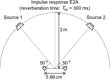
Fig. 3: Recording conditions of impulse responses obtained from RWCP database.

Table 2: Relative computational times normalized by AuxIVA

Method	Two-source case	Three-source case
AuxIVA [5]	1.00	1.00
Proposed $t$-ILRMA	1.46	1.40
$t$-MNMF [14]	8.83	74.51

By iteratively calculating the update rules (16), (17), (22), and (23), the cost function (8) monotonically decreases, and the convergence is theoretically guaranteed. However, a scale ambiguity exists in the estimated signal $y_{ij,n}$ in ILRMA, and $\bm{W}_{i}$, $t_{il,n}$, and $v_{lj,n}$ should be normalized in each iteration as

$$\bm{w}_{i,n}\leftarrow \ \bm{w}_{i,n}\eta_{n}^{-1},$$ (24)

$$y_{ij,n}\leftarrow \ y_{ij,n}\eta_{n}^{-1},$$ (25)

$$\sigma_{ij,n}^{p}\leftarrow \ \sigma_{ij,n}^{p}\eta_{n}^{-p},$$ (26)

$$t_{il,n}\leftarrow \ t_{il,n}\eta_{n}^{-p},$$ (27)

where $\eta_{n}$ is an arbitrary sourcewise normalization coefficient, such as the sourcewise average power

$$\eta_{n}=\sqrt{\frac{1}{IJ}\sum_{i,j}|y_{ij,n}|^{2}}.$$ (28)

The signal scale of $y_{ij,n}$ can easily be restored by applying a back-projection technique after the cost function has converged, as

$$\hat{\bm{y}}_{ij,n}=\bm{W}_{i}^{-1}\left(\bm{e}_{n}\circ\bm{y}_{ij}\right),$$ (29)

where $\hat{\bm{y}}_{ij,n}$ is a scale-restored estimated source image and $\circ$ denotes element-wise multiplication. The algorithm for $t$-ILRMA is summarized in Algorithm 1.

4 Experiments

4.1 Conditions

We confirmed the validity of the proposed generalization of ILRMA by conducting a BSS experiment using music and speech mixtures. The dry sources were obtained from SiSEC2011 [18] and are shown in Table 1. To simulate a reverberant mixture, the mixture signals were produced by convoluting the impulse response E2A ($T_{60}\!=\!300$ ms), which was obtained from the RWCP database [19], with each source. The recording conditions of the impulse responses are shown in Fig. 3. The initial demixing matrix $\bm{W}_{i}$ was always set to the identity matrix, and the NMF parameters $t_{il,n}$ and $v_{lj,n}$ were initialized by random values. An STFT was performed using a 512-ms-long Hamming window with a 128 ms shift. The number of bases $L$ was set to five for music signals and two for speech signals, and the update rules were iterated 200 times. As the evaluation score, we used the signal-to-distortion ratio (SDR) [20], which indicates the overall separation quality.

4.2 Computational times compared with those of $t$-MNMF

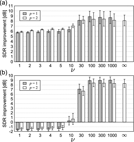
Fig. 4: SDR improvements of conventional ILRMA and $t$-ILRMA: (a) Music 3 and (b) Speech 4.

Table 3: Average SDR improvements [dB] of $t$-ILRMA for music and speech signals

$\nu$	Music ($p\!=\!1$)	Music ($p\!=\!2$)	Speech ($p\!=\!1$)	Speech ($p\!=\!2$)
1	3.48	3.32	-0.18	-0.15
2	3.56	3.44	-0.24	-0.22
3	3.58	3.50	-0.26	-0.22
4	3.62	3.61	-0.29	-0.30
5	3.82	3.99	-0.30	-0.30
10	5.65	6.16	-0.13	-0.19
30	11.57	11.02	3.71	3.44
100	13.09	12.66	7.58	6.87
300	13.22	12.78	7.55	7.18
1000	13.27	12.76	7.74	7.09
$\infty$	-	12.89	-	6.72

To clarify the advantage of ILRMA-based BSS in a determined situation ($N\!=\!M$), we compared the computational times of $t$-ILRMA and $t$-MNMF. The update calculation for the NMF parameters in each algorithm is almost the same, but the estimation of the spatial parameter ($\bm{W}_{i}$ for $t$-ILRMA and the spatial covariance for $t$-MNMF) is different. Although $t$-ILRMA requires one inverse of $\bm{W}_{i}\bm{U}_{i,n}$ for each $i$ and $n$, $t$-MNMF requires $J$ inverses and two eigenvalue decompositions of the $M\!\times\!M$ matrix. Table 2 shows an example of relative computational times normalized by that of AuxIVA [5], where we used MATLAB 9.2 (64-bit) with an AMD Ryzen 7 1800X (8 cores and 3.6 GHz) CPU. From this table, we can confirm that the computational time of $t$-ILRMA does not increase significantly compared with that of IVA, whereas that of $t$-MNMF markedly increases. $t$-ILRMA was about six times faster than $t$-MNMF in the two-source case and about $53$ times faster in the three-source case.

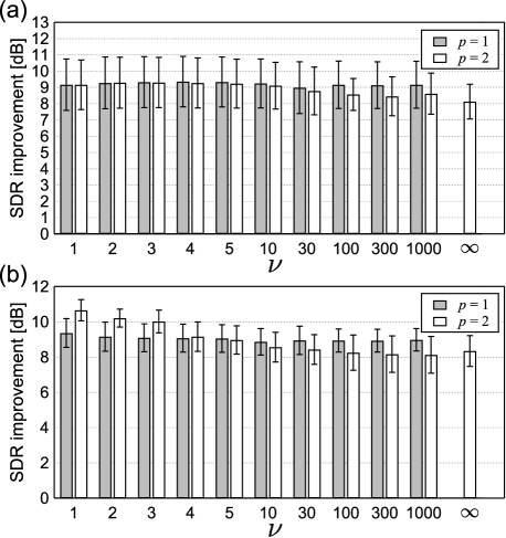
Fig. 5: SDR improvements of conventional ILRMA and $t$-ILRMA with initialization: (a) Music 3 and (b) Speech 4.

Table 4: Average SDR improvements [dB] of $t$-ILRMA with initialization for music and speech signals

$\nu$	Music ($p\!=\!1$)	Music ($p\!=\!2$)	Speech ($p\!=\!1$)	Speech ($p\!=\!2$)
1	13.15	13.09	6.93	7.11
2	13.31	13.27	6.97	7.01
3	13.34	13.39	6.89	6.97
4	13.27	13.26	6.99	6.85
5	13.25	13.32	6.94	6.89
10	13.41	13.38	7.04	6.87
30	13.39	13.33	7.25	6.78
100	13.39	13.35	7.29	6.82
300	13.39	13.27	7.21	6.83
1000	13.38	13.32	7.19	6.84
$\infty$	-	12.89	-	6.72

4.3 Results with random initialization

Fig. 4 shows an example of average SDR improvements and their standard deviations for various values of $\nu$, where the separation was performed 10 times with different random initializations for the parameters. Note that the result for $\nu\!\rightarrow\!\infty$ and $p\!=\!2$ corresponds to that for the conventional ILRMA assuming a complex Gaussian source generative model. From this result, we can confirm that the separation performance becomes stable and robust for the random initialization when $\nu$ is set to a small value. However, the performance is degraded for both music and speech signals when $\nu\!\leq\!10$. Only for the signals in Fig. 4 does the proposed method with $(\nu,p)\!=\!(100,1)$ for the music signal and $(\nu,p)\!=\!(1000,1)$ for the speech signal provide the best separation score. However, this tendency can vary with the dataset, namely, the optimal value of $\nu$ depends on the instrument or the speaker in the mixture signal. Table 3 shows the average scores of all music or speech signals. We can confirm that a higher value of $\nu$ and $p\!=\!1$ are always preferable for the separation.

4.4 Results with conventional ILRMA initialization

When $\nu$ is small, the Student’s $t$-distribution approaches the Cauchy distribution, where the latter can ignore outlier components. In particular, Cauchy NMF is suitable for extracting significant bases from a truly low-rank data matrix contaminated by outlier noise [9]. In the early stage of $t$-ILRMA iterations, the estimated spectrogram $|\bm{Y}_{n}|^{.p}$ includes almost all the source components because the initial demixing matrix is set to the identity matrix, and it is not a low-rank matrix even though each source spectrogram $|\bm{S}_{n}|^{.p}$ is truly low-rank. In such a case, $t$-ILRMA with a small value of $\nu$, such as Cauchy NMF, may not extract the useful bases for BSS, and the optimization will be trapped at a poor solution.

To solve this problem, in this experiment, we apply conventional ILRMA ($t\!\rightarrow\!\infty$) in the early stage of iterations, then $t$-ILRMA with an arbitrary $\nu$ is applied in the late stage, where for $t$-ILRMA, the bases and activations are pretrained using the outputs of conventional ILRMA via $t$-NMF. Fig. 5 and Table 4 show the average results of this approach, where conventional ILRMA is performed for the first 100 iterations and $t$-ILRMA is applied for the last 100 iterations. Compared with the previous results, a smaller value of $\nu$ tends to provide better results and to outperform conventional ILRMA, although the stability is not improved because of the conventional-ILRMA-based initialization.

5 Conclusion

In this paper, we generalized the source distribution assumed in ILRMA from a complex Gaussian distribution to a complex Student’s $t$-distribution, which allows us to control the robustness to outlier components and includes the Cauchy distribution when $\nu\!=\!1$. The proposed $t$-ILRMA can outperform conventional ILRMA with an appropriate value of $\nu$. Also, initialization with a Gaussian assumption leads to further improvement for both music and speech BSS tasks.

6 Acknowledgment

This work was partly supported by ImPACT Program of Council for Science, SECOM Science and Technology Foundation, and JSPS KAKENHI Grant Number16H01735.

References

- [1] P. Comon, “Independent component analysis, a new concept?,” Signal Process., vol. 36, no. 3, pp. 287–314, 1994.
- [2] P. Smaragdis, “Blind separation of convolved mixtures in the frequency domain,” Neurocomputing, vol. 22, no. 1, pp. 21–34, 1998.
- [3] H. Saruwatari, T. Kawamura, T. Nishikawa, A. Lee, and K. Shikano, “Blind source separation based on a fast-convergence algorithm combining ICA and beamforming,” IEEE Trans. ASLP, vol. 14, no. 2, pp. 666–678, 2006.
- [4] T. Kim, H. T. Attias, S.-Y. Lee, and T.-W. Lee, “Blind source separation exploiting higher-order frequency dependencies,” IEEE Trans. ASLP, vol. 15, no. 1, pp. 70–79, 2007.
- [5] N. Ono, “Stable and fast update rules for independent vector analysis based on auxiliary function technique,” in Proc. WASPAA, 2011, pp. 189–192.
- [6] D. R. Hunter and K. Lange, “Quantile regression via an MM algorithm,” Journal of Computational and Graphical Statistics, vol. 9, no. 1, pp. 60–77, 2000.
- [7] D. D. Lee and H. S. Seung, “Learning the parts of objects by non-negative matrix factorization,” Nature, vol. 401, no. 6755, pp. 788–791, 1999.
- [8] C. Févotte, N. Bertin, and J.-L. Durrieu, “Nonnegative matrix factorization with the Itakura–Saito divergence. With application to music analysis,” Neural Computation, vol. 21, no. 3, pp. 793–830, 2009.
- [9] A. Liutkus, D. FitzGerald, and R. Badeau, “Cauchy nonnegative matrix factorization,” in Proc. WASPAA, 2015.
- [10] K. Yoshii, K. Itoyama, and M. Goto, “Student’s t nonnegative matrix factorization and positive semidefinite tensor factorization for single-channel audio source separation,” in Proc. ICASSP, 2016, pp. 51–55.
- [11] A. Ozerov and C. Févotte, “Multichannel nonnegative matrix factorization in convolutive mixtures for audio source separation,” IEEE Trans. ASLP, vol. 18, no. 3, pp. 550–563, 2010.
- [12] H. Kameoka, T. Yoshioka, M. Hamamura, J. L. Roux, and K. Kashino, “Statistical model of speech signals based on composite autoregressive system with application to blind source separation,” in Proc. LVA/ICA, 2010, pp. 245–253.
- [13] H. Sawada, H. Kameoka, S. Araki, and N. Ueda, “Multichannel extensions of non-negative matrix factorization with complex-valued data,” IEEE Trans. ASLP, vol. 21, no. 5, pp. 971–982, 2013.
- [14] K. Kitamura, Y. Bando, K. Itoyama, and K. Yoshii, “Student’s multichannel nonnegative matrix factorization for blind source separation,” in Proc. IWAENC, 2016.
- [15] D. Kitamura, N. Ono, H. Sawada, H. Kameoka, and H. Saruwatari, “Determined blind source separation unifying independent vector analysis and nonnegative matrix factorization,” IEEE/ACM Trans. ASLP, vol. 24, no. 9, pp. 1626–1641, 2016.
- [16] Y. Mitsui, D. Kitamura, S. Takamichi, N. Ono, and H. Saruwatari, “Blind source separation based on independent low-rank matrix analysis with sparse regularization for time-series activity,” in Proc. ICASSP, 2017, pp. 21–25.
- [17] A. Yeredor, “On hybrid exact-approximate joint diagonalization,” in Proc. CAMSAP, 2009, pp. 312–315.
- [18] S. Araki, F. Nesta, E. Vincent, Z. Koldovský, G. Nolte, A. Ziehe, and A. Benichoux, “The 2011 signal separation evaluation campaign (SiSEC2011):-audio source separation,” in Proc. LVA/ICA, 2012, pp. 414–422.
- [19] S. Nakamura, K. Hiyane, F. Asano, T. Nishiura, and T. Yamada, “Acoustical sound database in real environments for sound scene understanding and hands-free speech recognition,” in Proc. LREC, 2000, pp. 965–968.
- [20] E. Vincent, R. Gribonval, and C. Févotte, “Performance measurement in blind audio source separation,” IEEE Trans. ASLP, vol. 14, no. 4, pp. 1462–1469, 2006.