Some remarks on the theorems of Wright and Braaksma on the Wright function ${}_{p}\Psi_{q}(z)$

Abstract

We carry out a numerical investigation of the asymptotic expansion of the so-called Wright function ${}_{p}\Psi_{q}(z)$ (a generalised hypergeometric function) in the case when exponentially small terms are present. This situation is covered by two theorems of Wright and Braaksma. We demonstrate that a more precise understanding of the behaviour of ${}_{p}\Psi_{q}(z)$ is obtained by taking into account the Stokes phenomenon.

  

1.   Introduction

We consider the Wright function (a generalised hypergeometric function) defined by

$${}_{p}\Psi_{q}(z)\equiv{}_{p}\Psi_{q}\biggl{(}\!\!\begin{array}[]{c}(\alpha_{1},a_{1}),\ldots,(\alpha_{p},a_{p})\\ (\beta_{1},b_{1}),\ldots,(\beta_{q},b_{q})\end{array}\!\!;z\!\biggr{)}=\sum_{n=0}^{\infty}g(n)\,\frac{z^{n}}{n!},$$ (1.1)

$$g(n)=\frac{\prod_{r=1}^{p}\Gamma(\alpha_{r}n+a_{r})}{\prod_{r=1}^{q}\Gamma(\beta_{r}n+b_{r})},$$ (1.2)

where $p$ and $q$ are nonnegative integers, the parameters $\alpha_{r}$ and $\beta_{r}$ are real and positive and $a_{r}$ and $b_{r}$ are arbitrary complex numbers. We also assume that the $\alpha_{r}$ and $a_{r}$ are subject to the restriction

$$\alpha_{r}n+a_{r}\neq 0,-1,-2,\ldots\qquad(n=0,1,2,\ldots\ ;\,1\leq r\leq p)$$ (1.3)

so that no gamma function in the numerator in (1.1) is singular. In the special case $\alpha_{r}=\beta_{r}=1$, the function ${}_{p}\Psi_{q}(z)$ reduces to a multiple of the ordinary hypergeometric function

$${}_{p}\Psi_{q}(z)=\frac{\prod_{r=1}^{p}\Gamma(a_{r})}{\prod_{r=1}^{q}\Gamma(b_{r})}\,{}_{p}F_{q}\biggl{(}\begin{array}[]{c}a_{1},\ldots,a_{p}\\ b_{1},\ldots,b_{q}\end{array}\!\!;z\biggr{)};$$

see, for example, [13, p. 40].

We introduce the parameters associated with $g(n)$ given by

$$\kappa=1+\sum_{r=1}^{q}\beta_{r}-\sum_{r=1}^{p}\alpha_{r},\qquad h=\prod_{r=1}^{p}\alpha_{r}^{\alpha_{r}}\prod_{r=1}^{q}\beta_{r}^{-\beta_{r}},$$

$$\vartheta=\sum_{r=1}^{p}a_{r}-\sum_{r=1}^{q}b_{r}+\leavevmode\hbox{${\textstyle\frac{1}{2}}$}(q-p),\qquad\vartheta^{\prime}=1-\vartheta.$$ (1.4)

If it is supposed that $\alpha_{r}$ and $\beta_{r}$ are such that $\kappa>0$ then ${}_{p}\Psi_{q}(z)$ is uniformly and absolutely convergent for all finite $z$. If $\kappa=0$, the sum in (1.1) has a finite radius of convergence equal to $h^{-1}$, whereas for $\kappa<0$ the sum is divergent for all nonzero values of $z$. The parameter $\kappa$ will be found to play a critical role in the asymptotic theory of ${}_{p}\Psi_{q}(z)$ by determining the sectors in the $z$-plane in which its behaviour is either exponentially large, algebraic or exponentially small in character as $|z|\rightarrow\infty$.

The determination of the asymptotic expansion of ${}_{p}\Psi_{q}(z)$ for $|z|\rightarrow\infty$ and finite values of the parameters has a long history; for details, see [10, §2.3]. Detailed investigations were carried out by Wright [16, 17] and by Braaksma [2] for a more general class of integral functions than (1.1). We present a summary of their results related to the asymptotic expansion of ${}_{p}\Psi_{q}(z)$ for large $|z|$ in Section 2. Our purpose here is to consider two of the expansion theorems involving the presence of exponentially small expansions valid in certain sectors of the $z$-plane. We demonstrate by numerical computation that a more precise understanding of the asymptotic structure of ${}_{p}\Psi_{q}(z)$ can be achieved by taking into account the Stokes phenomenon.

2.  Standard asymptotic theory for $|z|\rightarrow\infty$

We first state the standard asymptotic expansion of the integral function ${}_{p}\Psi_{q}(z)$ as $|z|\rightarrow\infty$ for $\kappa>0$ and finite values of the parameters given in [17] and [2]; see also [11, §2.3]. To present this expansion we introduce the exponential expansion $E_{p,q}(z)$ and the algebraic expansion $H_{p,q}(z)$ associated with ${}_{p}\Psi_{q}(z)$.

The exponential expansion $E_{p,q}(z)$ can be obtained from the Ford-Newsom theorem [3, 4]. A simpler derivation of this result in the case ${}_{p}\Psi_{q}(z)$ based on the Abel-Plana form of the well-known Euler-Maclaurin summation formula is given in [10, pp. 42–50]. We have the formal asymptotic sum

$$E_{p,q}(z):=Z^{\vartheta}e^{Z}\sum_{j=0}^{\infty}A_{j}Z^{-j},\qquad Z=\kappa(hz)^{1/\kappa},$$ (2.1)

where the coefficients $A_{j}$ are those appearing in the inverse factorial expansion of $g(s)/s!$ given by

$$\frac{g(s)}{\Gamma(1+s)}=\kappa(h\kappa^{\kappa})^{s}\biggl{\{}\sum_{j=0}^{M-1}\frac{A_{j}}{\Gamma(\kappa s+\vartheta^{\prime}+j)}+\frac{\rho_{M}(s)}{\Gamma(\kappa s+\vartheta^{\prime}+M)}\biggr{\}}.$$ (2.2)

Here $g(s)$ is defined in (1.2) with $n$ replaced by $s$, $M$ is a positive integer and $\rho_{M}(s)=O(1)$ for $|s|\rightarrow\infty$ in $|\arg\,s|<\pi$. The leading coefficient $A_{0}$ is specified by

$$A_{0}=(2\pi)^{\frac{1}{2}(p-q)}\kappa^{-\frac{1}{2}-\vartheta}\prod_{r=1}^{p}\alpha_{r}^{a_{r}-\frac{1}{2}}\prod_{r=1}^{q}\beta_{r}^{\frac{1}{2}-b_{r}}.$$ (2.3)

The coefficients $A_{j}$ are independent of $s$ and depend only on the parameters $p$, $q$, $\alpha_{r}$, $\beta_{r}$, $a_{r}$ and $b_{r}$. An algorithm for their evaluation is described in the appendix.

The algebraic expansion $H_{p,q}(z)$ follows from the Mellin-Barnes integral representation [11, §2.4]

$${}_{p}\Psi_{q}(z)=\frac{1}{2\pi i}\int_{-\infty i}^{\infty i}\Gamma(s)g(-s)(ze^{\mp\pi i})^{-s}ds,\qquad|\arg(-z)|<\pi(1-\leavevmode\hbox{${\textstyle\frac{1}{2}}$}\kappa),$$ (2.4)

where the path of integration is indented near $s=0$ to separate the poles of $\Gamma(s)$ from those of $g(-s)$ situated at

$$s=(a_{r}+k)/\alpha_{r},\qquad k=0,1,2,\dots\,\ (1\leq r\leq p).$$ (2.5)

In general there will be $p$ such sequences of simple poles though, depending on the values of $\alpha_{r}$ and $a_{r}$, some of these poles could be multiple poles or even ordinary points if any of the $\Gamma(\beta_{r}s+b_{r})$ are singular there. Displacement of the contour to the right over the poles of $g(-s)$ then yields the algebraic expansion of ${}_{p}\Psi_{q}(z)$ valid in the sector in (2.4).

If it is assumed that the parameters are such that the poles in (2.5) are all simple we obtain the algebraic expansion given by $H_{p,q}(z)$, where

$$H_{p,q}(z):=\sum_{m=1}^{p}\alpha_{m}^{-1}z^{-a_{m}/\alpha_{m}}S_{p,q}(z;m)$$ (2.6)

and $S_{p,q}(z;m)$ denotes the formal asymptotic sum

$$S_{p,q}(z;m):=\sum_{k=0}^{\infty}\frac{(-)^{k}}{k!}\Gamma\left(\frac{k+a_{m}}{\alpha_{m}}\right)\,\frac{\prod_{r=1}^{{}^{\prime}\,p}\Gamma(a_{r}-\alpha_{r}(k+a_{m})/\alpha_{m})}{\prod_{r=1}^{q}\Gamma(b_{r}-\beta_{r}(k+a_{m})/\alpha_{m})}z^{-k/\alpha_{m}},$$ (2.7)

with the prime indicating the omission of the term corresponding to $r=m$ in the product. This expression in (2.6) consists of (at most) $p$ expansions each with the leading behaviour $z^{-a_{m}/\alpha_{m}}$ ($1\leq m\leq p$). When the parameters $\alpha_{r}$ and $a_{r}$ are such that some of the poles are of higher order, the expansion (2.7) is invalid and the residues must then be evaluated according to the multiplicity of the poles concerned; this will lead to terms involving $\log\,z$ in the algebraic expansion.

The three main expansion theorems are as follows. Throughout we let $\epsilon$ denote an arbitrarily small positive quantity.

Theorem 1

$\!\!\!.$ If $0<\kappa<2$, then

$${}_{p}\Psi_{q}(z)\sim\left\{\begin{array}[]{lll}E_{p,q}(z)+H_{p,q}(ze^{\mp\pi i})&\leavevmode\hbox{in}&|\arg\,z|\leq\leavevmode\hbox{${\textstyle\frac{1}{2}}$}\pi\kappa\\ \\ H_{p,q}(ze^{\mp\pi i})&\leavevmode\hbox{in}&\leavevmode\hbox{${\textstyle\frac{1}{2}}$}\pi\kappa+\epsilon\leq|\arg\,z|\leq\pi\end{array}\right.$$ (2.8)

as $|z|\rightarrow\infty$. The upper or lower sign in $H_{p,q}(ze^{\mp\pi i})$ is chosen according as $\arg\,z>0$ or $\arg\,z<0$, respectively.

It is seen that the $z$-plane is divided into two sectors, with a common vertex at $z=0$, by the rays $\arg\,z=\pm\leavevmode\hbox{${\textstyle\frac{1}{2}}$}\pi\kappa$. In the sector $|\arg\,z|<\leavevmode\hbox{${\textstyle\frac{1}{2}}$}\pi\kappa$, the asymptotic character of ${}_{p}\Psi_{q}(z)$ is exponentially large whereas in the complementary sector $\leavevmode\hbox{${\textstyle\frac{1}{2}}$}\pi\kappa<|\arg\,z|\leq\pi$, the dominant expansion of ${}_{p}\Psi_{q}(z)$ is algebraic in character. On the rays $\arg\,z=\pm\leavevmode\hbox{${\textstyle\frac{1}{2}}$}\pi\kappa$ the exponential expansion is oscillatory and is of a comparable magnitude to $H_{p,q}(ze^{\mp\pi i})$.

Theorem 2

$\!\!\!.$ If $\kappa=2$ then

$${}_{p}\Psi_{q}(z)\sim E_{p,q}(z)+E_{p,q}(ze^{\mp 2\pi i})+H_{p,q}(ze^{\mp\pi i})$$ (2.9)

as $|z|\to\infty$ in the sector $|\arg\,z|\leq\pi$. The upper or lower signs are chosen according as $\arg\,z>0$ or $\arg\,z<0$, respectively.

The rays $\arg\,z=\pm\leavevmode\hbox{${\textstyle\frac{1}{2}}$}\pi\kappa$ now coincide with the negative real axis. It follows that ${}_{p}\Psi_{q}(z)$ is exponentially large in character as $|z|\to\infty$ except in the neighbourhood of the negative real axis, where the algebraic expansion becomes asymptotically significant.

Theorem 3

$\!\!\!.$ When $\kappa>2$ we have

$${}_{p}\Psi_{q}(z)\sim\sum_{n=-N}^{N}E_{p,q}(ze^{2\pi in})+H_{p,q}(ze^{\mp\pi iz})$$ (2.10)

as $|z|\to\infty$ in the sector $|\arg\,z|\leq\pi$. The integer $N$ is chosen such that it is the smallest integer satisfying $2N+1>\leavevmode\hbox{${\textstyle\frac{1}{2}}$}\kappa$ and the upper or lower is chosen according as $\arg\,z>0$ or $\arg\,z<0$, respectively.

In this case the asymptotic behaviour of ${}_{p}\Psi_{q}(z)$ is exponentially large for all values of $\arg\,z$ and, consequently, the algebraic expansion may be neglected. The sums $E_{p,q}(ze^{2\pi in})$ are exponentially large (or oscillatory) as $|z|\to\infty$ for values of $\arg\,z$ satisfying $|\arg\,z+2\pi n|\leq\leavevmode\hbox{${\textstyle\frac{1}{2}}$}\pi\kappa$.

The division of the $z$-plane into regions where ${}_{p}\Psi_{q}(z)$ possesses exponentially large or algebraic behaviour for large $|z|$ is illustrated in Fig. 1. When $0<\kappa<2$, the exponential expansion $E_{p,q}(z)$ is still present in the sectors $\leavevmode\hbox{${\textstyle\frac{1}{2}}$}\pi\kappa<|\arg\,z|<\min\{\pi,\pi\kappa\}$, where it is subdominant. The rays $\arg\,z=\pm\pi\kappa$ ($0<\kappa<1$), where $E_{p,q}(z)$ is maximally subdominant with respect to $H_{p,q}(ze^{\mp\pi i})$, are called Stokes lines. As these rays are crossed (in the sense of increasing $|\arg\,z|$) the exponential expansion switches off according to Berry’s now familiar error-function smoothing law [1]; see [8] for details. The rays $\arg\,z=\pm\leavevmode\hbox{${\textstyle\frac{1}{2}}$}\pi\kappa$, where $E_{p,q}(z)$ is oscillatory and comparable to $H_{p,q}(ze^{\mp\pi i})$, are called anti-Stokes lines.

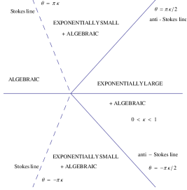
Figure 1: The exponentially large and algebraic sectors associated with ${}_{p}\Psi_{q}(z)$ in the complex $z$-plane with $\theta=\arg\,z$ when $0<\kappa<1$. The Stokes and anti-Stokes lines are indicated.

In view of the above interpretation of the Stokes phenomenon a more precise version of Theorem 1 is as follows:

Theorem 4

$\!\!\!.$ When $0<\kappa\leq 2$, then

$${}_{p}\Psi_{q}(z)\sim\left\{\begin{array}[]{lll}E_{p,q}(z)+H_{p,q}(ze^{\mp\pi i})&\leavevmode\hbox{in}&|\arg\,z|\leq\min\{\pi-\epsilon,\pi\kappa-\epsilon\}\\ \\ H_{p,q}(ze^{\mp\pi i})&\leavevmode\hbox{in}&\pi\kappa+\epsilon\leq|\arg\,z|\leq\pi\ \ (0<\kappa<1)\\ \\ E_{p,q}(z)+E_{p,q}(ze^{\mp 2\pi i})+H_{p,q}(ze^{\mp\pi i})&\leavevmode\hbox{in}&|\arg\,z|\leq\pi\ \ (1<\kappa\leq 2)\end{array}\right.$$ (2.11)

as $|z|\rightarrow\infty$. The upper or lower signs are chosen according as $\arg\,z>0$ or $\arg\,z<0$, respectively.

We omit the expansion on the Stokes lines $\arg\,z=\pm\pi\kappa$; the details in the case $p=1$, $q\geq 0$ are discussed in [9]. The expansions in (2.11a) and (2.8a) were given by Wright [16, 17] in the sector $|\arg\,z|\leq\min\{\pi,\leavevmode\hbox{${\textstyle\frac{3}{2}}$}\pi\kappa-\epsilon\}$ as he did not take into account the Stokes phenomenon. Since $E_{p,q}(z)$ is exponentially small in $\leavevmode\hbox{${\textstyle\frac{1}{2}}$}\pi\kappa<|\arg\,z|\leq\pi$, then in the sense of Poincaré, the expansion $E_{p,q}(z)$ can be neglected and there is no inconsistency between Theorems 1 and 4. Similarly, $E_{p,q}(ze^{-2\pi i})$ is exponentially small compared to $E_{p,q}(z)$ in $0\leq\arg\,z<\pi$ and there is no inconsistency between the expansions in (2.8a) and (2.11c) when $1<\kappa<2$. However, in the vicinity of $\arg\,z=\pi$, these last two expansions are of comparable magnitude and, for real parameters, they combine to generate a real result on this ray. A similar remark applies to $E_{p,q}(ze^{2\pi i})$ in $-\pi<\arg\,z\leq 0$.

The following theorem was given by Braaksma [2, p. 331].

Theorem 5

$\!\!\!.$ If $p=0$, so that $g(s)$ has no poles and $\kappa>1$, then $H_{0,q}(z)\equiv 0$. When $1<\kappa<2$, we have the expansion

$${}_{0}\Psi_{q}(z)\sim E_{0,q}(z)+E_{0,q}(ze^{\mp 2\pi i})$$ (2.12)

as $|z|\to\infty$ in the sector $|\arg\,z|\leq\pi$ The upper or lower sign is chosen according as $\arg\,z>0$ or $\arg\,z<0$, respectively. The dominant expansion ${}_{0}\Psi_{q}(z)\sim E_{p,q}(z)$ holds in the reduced sector $|\arg\,z|\leq\pi-\epsilon$.

It can be seen that (2.12) agrees with (2.11c) when $H_{p,q}(z)\equiv 0$. Braaksma gave the result (2.12) valid in a sector straddling the negative real axis given by $\pi-\delta\leq\arg\,z\leq\pi+\delta$, where $0<\delta<\leavevmode\hbox{${\textstyle\frac{1}{2}}$}\pi(1-\leavevmode\hbox{${\textstyle\frac{1}{2}}$}\kappa)$.

It is our purpose here to examine Theorems 4 and 5 in more detail by means of a series of examples. We carry out a numerical investigation to show that (2.11c) is valid when $1<\kappa<2$ and, when $0<\kappa<1$, that the exponential expansion $E_{p,q}(z)$ in Theorem 4 switches off (as $|\arg\,z|$ increases) across the Stokes lines $\arg\,z=\pm\pi\kappa$, where $E_{p,q}(z)$ is maximally subdoiminant with respect to $H_{p,q}(ze^{\mp\pi i})$. Similarly in Theorem 5, we show that when $1<\kappa<2$ the expansions $E_{p,q}(ze^{\mp 2\pi i})$ switch off across the Stokes lines $\arg\,z=\pm\pi(1-\leavevmode\hbox{${\textstyle\frac{1}{2}}$}\kappa)$, where they are maximally subdominant with respect to $E_{p,q}(z)$. Thus, although the expansions in (2.11a) and (2.12) are valid asymptotic descriptions, more accurate evaluation will result from taking into account the Stokes phenomenon as the above-mentioned rays are crossed.

3. Numerical examples

Example 3.1   Our first example is the Mittag-Leffler function ${\cal E}_{a,b}(z)$ defined by

$${\cal E}_{a,b}(z)=\sum_{n=0}^{\infty}\frac{z^{n}}{\Gamma(an+b)},$$

where we consider $a>0$. This corresponds to a case of ${}_{1}\Psi_{1}(z)$ with the parameters $\kappa=a$, $h=a^{-a}$, $\vartheta=1-b$ and $g(s)=\Gamma(1+s)/\Gamma(as+b)$. Then from (2.1)–(2.3), we have $Z=z^{1/a}$, $A_{0}=1/a$ with $A_{j}=0$ for $j\geq 1$. The exponential and algebraic expansions are from (2.1), (2.6) and (2.7) given by

$$E_{1,1}(z)=\frac{1}{a}z^{(1-b)/a}\exp[z^{1/a}],\qquad H_{1,1}(ze^{\mp\pi i})=-\sum_{k=1}^{\infty}\frac{z^{-k}}{\Gamma(b-ak)}.$$

Then, from Theorems 2, 3 and 4 we obtain the following asymptotic expansions as $|z|\to\infty$.

(i) When $0<a<1$

$${\cal E}_{a,b}(z)\sim\left\{\begin{array}[]{ll}\displaystyle{\frac{1}{a}}z^{(1-b)/a}\exp[z^{1/a}]-\sum_{k=1}^{\infty}\displaystyle{\frac{z^{-k}}{\Gamma(b-ak)}}&(|\arg\,z|\leq\pi a-\epsilon)\\ -{\displaystyle\sum_{k=1}^{\infty}\frac{z^{-k}}{\Gamma(b-ak)}}&(\pi a+\epsilon\leq\arg\,z\leq\pi);\end{array}\right.$$ (3.1)

(ii) when $1<a<2$

$${\cal E}_{a,b}(z)\sim\left\{\begin{array}[]{ll}\displaystyle{\frac{1}{a}}z^{(1-b)/a}\exp[z^{1/a}]-\sum_{k=1}^{\infty}\displaystyle{\frac{z^{-k}}{\Gamma(b-ak)}}&(|\arg\,z|\leq\pi-\epsilon)\\ \displaystyle{\frac{1}{a}}z^{(1-b)/a}\exp[z^{1/a}]+\displaystyle{\frac{1}{a}}(ze^{\mp 2\pi i})^{(1-b)/a}\exp[(ze^{\mp 2\pi i})^{1/a}]&\\ -{\displaystyle\sum_{k=1}^{\infty}\frac{z^{-k}}{\Gamma(b-ak)}}&(|\arg\,z|\leq\pi);\end{array}\right.$$ (3.2)

(iii) when $a=2$

$${\cal E}_{a,b}(z)\sim\displaystyle{\frac{1}{a}}z^{(1-b)/a}\exp[z^{1/a}]+\displaystyle{\frac{1}{a}}(ze^{\mp 2\pi i})^{(1-b)/a}\exp[(ze^{\mp 2\pi i})^{1/a}]$$

$$-{\displaystyle\sum_{k=1}^{\infty}\frac{z^{-k}}{\Gamma(b-ak)}}\qquad\qquad(|\arg\,z|\leq\pi);\hskip 56.9055pt$$ (3.3)

(iv) when $a>2$

$${\cal E}_{a,b}(z)\sim\frac{1}{a}\sum_{n=-N}^{N}(ze^{2\pi in})^{(1-b)/a}\exp[z^{1/a}e^{2\pi in/a}]-\sum_{k=1}^{\infty}\frac{z^{-k}}{\Gamma(b-ak)}\qquad(|\arg\,z|\leq\pi),$$ (3.4)

where $N$ is the smallest integer satisfying $2N+1>\leavevmode\hbox{${\textstyle\frac{1}{2}}$}a$. The upper or lower signs are taken according as $\arg\,z>0$ or $\arg\,z<0$, respectively.

When $0<a<1$, it is established in [6] (see also [15]) that the exponential term $a^{-1}\exp[z^{1/a}]$ in (3.1a)is multiplied by the approximate factor involving the error function

$$\frac{1}{2}+\frac{1}{2}\leavevmode\hbox{erf}\biggl{[}\frac{(\pi a\mp\theta)}{a}\,\sqrt{\frac{|z|}{2}}\biggr{]}$$

as $|z|\to\infty$ in the neighbourhood of the Stokes lines $\theta=\arg\,z=\pm\pi a$, respectively, where it is maximally subdominant. This shows that the above exponential term indeed switches off in the familiar manner [1] as one crosses the Stokes lines in the sense of increasing $|\theta|$ and that consequently the expansion in (3.1a) is valid in $|\arg\,z|\leq\pi a-\epsilon$.

On the negative real axis we put $z=-x$, with $x>0$. From (3.2), we have when $1<a<2$

$${\cal E}_{a,b}(-x)\sim\frac{1}{a}(xe^{\pi i})^{(1-b)/a}\exp[x^{1/a}e^{\pi i/a}]+\frac{1}{a}(xe^{-\pi i})^{(1-b)/a}\exp[(x^{1/a}e^{-\pi i/a}]$$

$$\hskip 113.81102pt-\sum_{k=1}^{\infty}\frac{(-x)^{-k}}{\Gamma(b-ak)}$$

$$=F_{a,b}(x)-\sum_{k=1}^{\infty}\frac{(-x)^{-k}}{\Gamma(b-ak)},$$ (3.5)

as $x\to+\infty$, where

$$F_{a,b}(x)=\frac{2}{a}x^{(1-b)/a}\exp\biggl{[}x^{1/a}\cos\frac{\pi}{a}\biggr{]}\,\cos\biggl{[}x^{1/a}\sin\frac{\pi}{a}+\pi\frac{(1-b)}{a}\biggr{]}.$$ (3.6)

The presence of the additional exponential expansion $E_{1,1}(ze^{\mp 2\pi i})$ in (3.2) is seen to be essential in order to obtain a real result (when $b$ is real) on the negative $z$-axis.

Example 3.2   Our second example is the function

$$F_{1}(z)=\sum_{n=0}^{\infty}\frac{\Gamma(\leavevmode\hbox{${\textstyle\frac{1}{2}}$}n+a)}{\Gamma(n+b)}\,\frac{z^{n}}{n!}\qquad(\kappa=\leavevmode\hbox{${\textstyle\frac{3}{2}}$}),$$ (3.7)

where $a$ and $b$ are finite parameters, which corresponds to a case of ${}_{1}\Psi_{1}(z)$. The exponential expansion is

$$E_{1,1}(z)=Z^{\vartheta}e^{Z}\sum_{j=0}^{\infty}A_{j}Z^{-j},\qquad Z=\leavevmode\hbox{${\textstyle\frac{3}{2}}$}(hz)^{2/3},$$

where, from (2.3),

$$A_{0}=(\leavevmode\hbox{${\textstyle\frac{2}{3}}$})^{\vartheta+1/2}(\leavevmode\hbox{${\textstyle\frac{1}{2}}$})^{a-1/2}$$

and $\vartheta=a-b$, $h=2^{-1/2}$. An algorithm for the computation of the normalised coefficients $c_{j}=A_{j}/A_{0}$ is described in the appendix. In our computations we have employed $0\leq j\leq 40$; the first ten coefficients $c_{j}$ for $F_{1}(z)$ are listed in Table 1 for the particular case $a=\leavevmode\hbox{${\textstyle\frac{1}{4}}$}$ and $b=\leavevmode\hbox{${\textstyle\frac{3}{4}}$}$. From (2.6), the algebraic expansion is

$$H_{1,1}(ze^{\mp\pi i})=2\sum_{k=0}^{\infty}\frac{(-)^{k}\Gamma(2k+2a)}{k!\Gamma(b-2a-2k)}\,(ze^{\mp\pi i})^{-2k-2a}.$$

$j$	$c_{j}$	$j$	$c_{j}$
1	${\textstyle\frac{61}{192}}$	2	${\textstyle\frac{23161}{73728}}$
3	${\textstyle\frac{22783285}{42467328}}$	4	${\textstyle\frac{44604509425}{32614907904}}$
5	${\textstyle\frac{30375638199305}{6262062317568}}$	6	${\textstyle\frac{162721816250787605}{7213895789838336}}$
7	${\textstyle\frac{180090830597703240215}{1385067991648960512}}$	8	${\textstyle\frac{1889199431389108590226475}{2127464435172803346432}}$
9	${\textstyle\frac{25599447910539396612172829375}{3676258543978604182634496}}$	10	${\textstyle\frac{86726322340809175676137010099575}{1411683280887784006131646464}}$

Table 1: The normalised coefficients $c_{j}$ for $1\leq j\leq 10$ (with $c_{0}=1$) for the sum (3.7) when $a=\leavevmode\hbox{${\textstyle\frac{1}{4}}$}$ and $b=\leavevmode\hbox{${\textstyle\frac{3}{4}}$}$.

It is clearly sufficient for real parameters to consider values of $z$ satisfying $0\leq\arg\,z\leq\pi$ and this we do throughout this section. From Theorem 4, we obtain

$$F_{1}(z)=E_{1,1}(z)+E_{1,1}(ze^{-2\pi i})+H_{1,1}(ze^{-\pi i})$$

as $|z|\to\infty$ in $0\leq\arg\,z\leq\pi$, from which we see that $F_{1}(z)$ is exponentially large in the sector $|\arg\,z|<3\pi/4$. We have computed $F_{1}(z)$ for a value of $|z|$ and varying $\theta=\arg\,z$ in the range $0.7\pi\leq\theta\leq\pi$. In Table 2 we show the absolute values of

$\theta/\pi$	$|{\cal R}_{1}(z)|$	$|E_{1,1}(ze^{-2\pi i})|$
1.00	$6.283513\times 10^{-7}$	$6.283515\times 10^{-7}$
0.95	$6.605074\times 10^{-8}$	$6.605098\times 10^{-8}$
0.90	$8.190985\times 10^{-9}$	$8.190854\times 10^{-9}$
0.85	$1.226317\times 10^{-9}$	$1.225981\times 10^{-9}$
0.80	$2.263874\times 10^{-10}$	$2.261409\times 10^{-10}$
0.75	$5.240704\times 10^{-11}$	$5.236698\times 10^{-11}$
0.70	$1.573812\times 10^{-11}$	$1.546959\times 10^{-11}$

Table 2: Values of the absolute error ${\cal R}_{1}(z)$ in the computation of $F_{1}(z)$ using an optimal truncation of both $E_{1,1}(z)$ and $H_{1,1}(ze^{-\pi i})$ compared with $|E_{1,1}(ze^{-2\pi i})|$ as a function of $\theta$ for $z=100e^{i\theta}$, $a=\leavevmode\hbox{${\textstyle\frac{1}{4}}$}$ and $b=\leavevmode\hbox{${\textstyle\frac{3}{4}}$}$.

$${\cal R}_{1}(z)\equiv F_{1}(z)-E_{1,1}^{opt}(z)-H_{1,1}^{opt}(ze^{-\pi i})$$

compared with $|E_{1,1}(ze^{-2\pi i})|$ (which was computed for $0\leq j\leq 5$), where the superscript ‘opt’ denotes that both the asymptotic sums $E_{1,1}(z)$ and $H_{1,1}(ze^{-\pi i})$ are truncated at their respective optimal truncation points. The results clearly confirm that (i) the exponential expansion $E_{1,1}(z)$ is present in the algebraic sector $\leavevmode\hbox{${\textstyle\frac{3}{4}}$}\pi<\arg\,z\leq\pi$ and (ii) the subdominant expansion $E_{1,1}(ze^{-2\pi i})$ is present in (at least) the sector $0.7\pi\leq\theta\leq\pi$. It was not possible to penetrate very far into the exponentially large sector $|\arg\,z|<\leavevmode\hbox{${\textstyle\frac{3}{4}}$}\pi$, since the error in the computation of $E_{1,1}(z)$ — even at optimal truncation — swamps the algebraic and subdominant exponential expansions. Such a computation would require a hyperasymptotic evaluation of the dominant expansion on the lines of that described for the generalised Bessel function ${}_{0}\Psi_{1}(z)$ in Wong and Zhao [14].

Example 3.3   Consider the function

$$F_{2}(z)=\sum_{n=0}^{\infty}\frac{\Gamma(\leavevmode\hbox{${\textstyle\frac{2}{3}}$}n+a\,)z^{n}}{\Gamma(\leavevmode\hbox{${\textstyle\frac{1}{3}}$}n+b)\,n!}\qquad(\kappa=\leavevmode\hbox{${\textstyle\frac{2}{3}}$}).$$

According to Theorem 4, the expansion of $F_{2}(z)$ for large $|z|$ is

$$F_{2}(z)\sim E_{1,1}(z)+H_{1,1}(ze^{-\pi i})\qquad(0\leq\arg\,z\leq\leavevmode\hbox{${\textstyle\frac{2}{3}}$}\pi-\epsilon).$$

The algebraic expansion is, from (2.6), given by

$$H_{1,1}(ze^{-\pi i})=\frac{3}{2}\sum_{k=0}^{\infty}\frac{(-)^{k}\Gamma(\leavevmode\hbox{${\textstyle\frac{3}{2}}$}k+\leavevmode\hbox{${\textstyle\frac{3}{2}}$}a)}{k!\,\Gamma(b-\leavevmode\hbox{${\textstyle\frac{1}{2}}$}a-\leavevmode\hbox{${\textstyle\frac{1}{2}}$}k)}(ze^{-\pi i})^{-3(k+a)/2}$$

and the exponential expansion $E_{1,1}(z)$ is obtained from (2.1) with the parameters $\vartheta=a-b$, $h=(\leavevmode\hbox{${\textstyle\frac{2}{3}}$})^{\frac{2}{3}}(\leavevmode\hbox{${\textstyle\frac{1}{3}}$})^{-\frac{1}{3}}$ and $A_{0}=\kappa^{-\frac{1}{2}-\vartheta}(\leavevmode\hbox{${\textstyle\frac{2}{3}}$})^{a-\frac{1}{2}}(\leavevmode\hbox{${\textstyle\frac{1}{3}}$})^{\frac{1}{2}-b}$. The coefficients $A_{j}$ are obtained as indicated in Example 3.2.

The function $F_{2}(z)$ is exponentially large in the sector $|\arg\,z|<\leavevmode\hbox{${\textstyle\frac{1}{3}}$}\pi$, whereas in the sector $\leavevmode\hbox{${\textstyle\frac{1}{3}}$}\pi<\arg\,z\leq\pi$ the algebraic expansion $H_{1,1}(ze^{-\pi i})$ is dominant. The expansion $E_{1,1}(z)$ is maximally subdominant with respect to $H_{1,1}(ze^{-\pi i})$ on the ray $\arg\,z=\pi\kappa=\leavevmode\hbox{${\textstyle\frac{2}{3}}$}\pi$. Consequently, as $\arg\,z$ increases, the exponential expansion $E_{1,1}(z)$ should switch off across the Stokes line $\arg\,z=\leavevmode\hbox{${\textstyle\frac{2}{3}}$}\pi$, to leave the algebraic expansion $H_{1,1}(ze^{-\pi i})$ in the sector $\leavevmode\hbox{${\textstyle\frac{2}{3}}$}\pi<\arg\,z\leq\pi$. To demonstrate this, we define the Stokes multiplier $S(\theta)$ by

$$F_{2}(z)=H_{11}^{opt}(ze^{-\pi i})+A_{0}Z^{\vartheta}e^{Z}\,S(\theta).$$

In Table 3 we show the absolute values of ${\cal R}_{2}(z):=F_{2}(z)-H_{1,1}^{opt}(ze^{-\pi i})$ and of the leading term of $E_{1,1}(z)$ as a function of $\theta=\arg\,z$. We also show the values of Re($S(\theta)$) in the neighbourhood of the Stokes line $\arg\,z=\leavevmode\hbox{${\textstyle\frac{2}{3}}$}\pi$ for the case $z=10e^{i\theta}$ and $a=\leavevmode\hbox{${\textstyle\frac{1}{3}}$}$, $b=\leavevmode\hbox{${\textstyle\frac{1}{4}}$}$. It is seen that the Stokes multiplier has the value $\simeq 1$ when $\theta=\leavevmode\hbox{${\textstyle\frac{1}{2}}$}\pi$ (before the transition commences) and $\simeq 0$ when $\theta=\leavevmode\hbox{${\textstyle\frac{3}{4}}$}\pi$ (after the transition is almost completed).

$\theta/\pi$	$|{\cal R}_{2}(z)|$	$|A_{0}Z^{\vartheta}e^{Z}|$	Re$(S(\theta))$
0.50	$4.4964\times 10^{-8}$	$4.4947\times 10^{-8}$	1.0000
0.55	$1.2980\times 10^{-9}$	$1.3005\times 10^{-9}$	0.9981
0.60	$1.1196\times 10^{-10}$	$1.1848\times 10^{-10}$	0.9450
0.62	$5.6361\times 10^{-11}$	$6.4685\times 10^{-11}$	0.8713
0.64	$3.2641\times 10^{-11}$	$4.3607\times 10^{-11}$	0.7485
0.66	$1.9737\times 10^{-11}$	$3.6426\times 10^{-11}$	0.5418
0.68	$1.3545\times 10^{-11}$	$3.7762\times 10^{-11}$	0.3600
0.70	$9.9952\times 10^{-12}$	$4.8568\times 10^{-11}$	0.2058
0.72	$9.1973\times 10^{-12}$	$7.7328\times 10^{-11}$	0.1189
0.75	$5.6314\times 10^{-12}$	$2.2959\times 10^{-10}$	0.0237

Table 3: Values of the absolute error in ${\cal R}_{2}(z)\equiv F_{2}(z)-H_{1,1}^{opt}(ze^{-\pi i})$ in the computation of $F_{2}(z)$ using an optimal truncation of the algebraic expansion compared with the leading term of $|E_{1,1}(z)|$ as a function of $\theta$ for $z=10e^{i\theta}$, $a=\leavevmode\hbox{${\textstyle\frac{1}{3}}$}$ and $b=\leavevmode\hbox{${\textstyle\frac{1}{4}}$}$. The final column shows the real part of the computed Stokes multiplier $S(\theta)$ for transition across the ray $\arg\,z=\leavevmode\hbox{${\textstyle\frac{2}{3}}$}\pi$.

Example 3.4   Our final example is the function of the type ${}_{0}\Psi_{2}(z)$ given by

$$F_{3}(z)=\sum_{n=0}^{\infty}\frac{z^{n}}{n!\Gamma(cn+a)\Gamma(cn+b)}\qquad(\kappa=1+2c),$$ (3.8)

where $0<c\leq\leavevmode\hbox{${\textstyle\frac{1}{2}}$}$. Since $p=0$, the algebraic expansion $H_{0,2}(z)\equiv 0$. From Theorem 5 we obtain the asymptotic expansion

$$F_{3}(z)\sim E_{0,2}(z)+E_{0,2}(ze^{\mp 2\pi i})\qquad(|\arg\,z|\leq\pi),$$

where the associated parameters are $\vartheta=1-a-b$, $h=c^{-2c}$ and

$$A_{0}=\frac{c^{\vartheta}\kappa^{-\vartheta-1/2}}{2\pi}~{}.$$

The function $F_{3}(z)$ is exponentially large in the sector $|\arg\,z|<\leavevmode\hbox{${\textstyle\frac{1}{2}}$}\pi(1+2c)$. The other expansion $E_{0,2}(ze^{-2\pi i})$ is subdominant in the upper half-plane but combines with $E_{0,2}(z)$ on the negative real axis to produce (for real $a$ and $b$) a real expansion.

Since the exponential factors associated with $E_{0,2}(z)$ and $E_{0,2}(ze^{-2\pi i})$ are $\exp[|Z|e^{i\theta/\kappa}]$ and $\exp[|Z|e^{i(\theta-2\pi)/\kappa}]$, where $\theta=\arg\,z$ and we recall that $Z$ is defined in (2.1), the greatest difference between these factors occurs when

$$\sin\biggl{(}\frac{\theta}{\kappa}\biggr{)}=\sin\biggl{(}\frac{\theta-2\pi}{\kappa}\biggr{)};$$

that is, when $\theta=\leavevmode\hbox{${\textstyle\frac{1}{2}}$}\pi(2-\kappa)$. Consequently, as $\arg\,z$ increases in the upper half-plane, we expect that the expansion $E_{0,2}(ze^{-2\pi i})$ should switch on across the Stokes line $\arg\,z=\leavevmode\hbox{${\textstyle\frac{1}{2}}$}\pi(2-\kappa)$; similar considerations apply to $E_{0,2}(ze^{2\pi i})$ and the Stokes line $\arg\,z=-\leavevmode\hbox{${\textstyle\frac{1}{2}}$}\pi(2-\kappa)$ in the lower half-plane.

To demonstrate the correctness of this claim, we choose $c=\leavevmode\hbox{${\textstyle\frac{1}{10}}$}$ (so that $\kappa=\leavevmode\hbox{${\textstyle\frac{6}{5}}$}$) and $a=\leavevmode\hbox{${\textstyle\frac{1}{4}}$}$, $b=\leavevmode\hbox{${\textstyle\frac{3}{4}}$}$. The function $F_{3}(z)$ is therefore exponentially large in the sector $|\arg\,z|<\leavevmode\hbox{${\textstyle\frac{3}{5}}$}\pi$ and the Stokes line in the upper half-plane is $\arg\,z=\leavevmode\hbox{${\textstyle\frac{2}{5}}$}\pi$. We have chosen $a-b$ to have a half-integer value for a very specific reason. The more detailed treatment in [8] shows that there is a third (subdominant) exponential series present in the expansion of $F_{3}(z)$ given by

$$2\cos\pi(a-b)\,X^{\vartheta}e^{-X}\sum_{j=0}^{\infty}A_{j}(-X)^{-j},\qquad X=\kappa(hze^{-\pi i})^{1/\kappa}.$$

Our present choice of $a$ and $b$ therefore eliminates this third expansion and enables us to deal with a case comprising only two exponential expansions.

In Table 4, we show for $|z|=20$ and varying $\theta=\arg\,z$ the values of $|F_{3}(z)-E_{0,2}^{opt}(z)|$ and $|E_{0,2}(ze^{-2\pi i})|$ together with the real part of the Stokes multiplier $S(\theta)$ defined by

$$F_{3}(z)=E_{0,2}^{opt}(z)+A_{0}(Ze^{-2\pi i/\kappa})^{\vartheta}\,\exp[Ze^{-2\pi i/\kappa}]\,S(\theta).$$

The results clearly demonstrate the switching-on of the subdominant expansion $E_{0,2}(ze^{-2\pi i})$ across the Stokes line $\arg\,z=\leavevmode\hbox{${\textstyle\frac{2}{5}}$}\pi$ as $\arg\,z$ increases in the upper half-plane.

$\theta/\pi$	$|{\cal R}_{3}(z)|$	$|E_{0,2}(ze^{-2\pi i})|$	Re$(S(\theta))$
0.20	$7.231938\times 10^{-4}$	$1.452127\times 10^{-1}$	0.0020
0.25	$2.204854\times 10^{-4}$	$8.898995\times 10^{-3}$	0.0184
0.30	$5.082653\times 10^{-5}$	$5.720603\times 10^{-4}$	0.0797
0.35	$9.416276\times 10^{-6}$	$4.042959\times 10^{-5}$	0.2230
0.40	$1.502207\times 10^{-6}$	$3.287009\times 10^{-6}$	0.4477
0.45	$2.239289\times 10^{-7}$	$3.209167\times 10^{-7}$	0.6893
0.50	$3.430029\times 10^{-8}$	$3.915246\times 10^{-8}$	0.8679
0.55	$5.977355\times 10^{-9}$	$6.187722\times 10^{-9}$	0.9575
0.60	$1.301304\times 10^{-9}$	$1.307416\times 10^{-9}$	0.9862
1.00	$1.307416\times 10^{-9}$	$1.307416\times 10^{-9}$	0.9908

Table 4: Values of the absolute error in ${\cal R}_{3}(z)\equiv F_{3}(z)-E_{0,2}^{opt}(z)$ in the computation of $F_{3}(z)$ using an optimal truncation of $E_{0,2}(z)$ compared with $|E_{0,2}(ze^{-2\pi i})|$ as a function of $\theta$ for $z=20e^{i\theta}$, $a=\leavevmode\hbox{${\textstyle\frac{1}{4}}$}$ and $b=\leavevmode\hbox{${\textstyle\frac{3}{4}}$}$. The final column shows the real part of the computed Stokes multiplier $S(\theta)$ for transition across the ray $\arg\,z=\leavevmode\hbox{${\textstyle\frac{2}{5}}$}\pi$.

Appendix:  An algorithm for the computation of the coefficients $c_{j}=A_{j}/A_{0}$

We describe an algorithm for the computation of the normalised coefficients $c_{j}=A_{j}/A_{0}$ appearing in the exponential expansion $E_{p,q}(z)$ in (2.1). Methods of computing these coefficients by recursion in the case $\alpha_{r}=\beta_{r}=1$ have been given by Riney [12] and Wright [18]; see [11, Section 2.2.2] for details. Here we describe an algebraic method for arbitrary $\alpha_{r}>0$ and $\beta_{r}>0$.

The inverse factorial expansion (2.2) can be re-written as

$$\frac{g(s)\Gamma(\kappa s+\vartheta^{\prime})}{\Gamma(1+s)}=\kappa A_{0}(h\kappa^{\kappa})^{s}\biggl{\{}\sum_{j=0}^{M-1}\frac{c_{j}}{(\kappa s+\vartheta^{\prime})_{j}}+\frac{O(1)}{(\kappa s+\vartheta^{\prime})_{M}}\biggr{\}}$$ (A.1)

for $|s|\to\infty$ uniformly in $|\arg\,s|\leq\pi-\epsilon$, where $g(s)$ is defined in (1.2) with $n$ replaced by $s$. Introduction of the scaled gamma function $\Gamma^{*}(z)=\Gamma(z)(2\pi)^{-\frac{1}{2}}e^{z}z^{\frac{1}{2}-z}$ leads to the representation

$$\Gamma(\alpha s+a)=(2\pi)^{\frac{1}{2}}e^{-\alpha s}(\alpha s)^{\alpha s+a-\frac{1}{2}}\,{\bf e}(\alpha s;a)\Gamma^{*}(\alpha s+a),$$

where

$${\bf e}(\alpha s;a):=e^{-a}\biggl{(}1+\frac{a}{\alpha s}\biggr{)}^{\alpha s+a-\frac{1}{2}}=\exp\,\left[(\alpha s+a-\leavevmode\hbox{${\textstyle\frac{1}{2}}$})\log\,\left(1+\frac{a}{\alpha s}\right)-a\right].$$

Then, after some routine algebra we find that the left-hand side of (A.1) can be written as

$$\frac{g(s)\Gamma(\kappa s+\vartheta^{\prime})}{\Gamma(1+s)}=\kappa A_{0}(h\kappa^{\kappa})^{s}\,R_{p,q}(s)\,\Upsilon_{p,q}(s),$$ (A.2)

where

$$\Upsilon_{p,q}(s):=\frac{\prod_{r=1}^{p}\Gamma^{*}(\alpha_{r}s+a_{r})}{\prod_{r=1}^{q}\Gamma^{*}(\beta_{r}s+b_{r})}\,\frac{\Gamma^{*}(\kappa s+\vartheta^{\prime})}{\Gamma^{*}(1+s)},\qquad R_{p,q}(s):=\frac{\prod_{r=1}^{p}e(\alpha_{r}s;a_{r})}{\prod_{r=1}^{q}e(\beta_{r}s;b_{r})}\,\frac{e(\kappa s;\vartheta^{\prime})}{e(s;1)}.$$

Substitution of (A.2) in (A.1) then yields the inverse factorial expansion in the form

$$R_{p,q}(s)\,\Upsilon_{p,q}(s)=\sum_{j=0}^{M-1}\frac{c_{j}}{(\kappa s+\vartheta^{\prime})_{j}}+\frac{O(1)}{(\kappa s+\vartheta^{\prime})_{M}}$$ (A.3)

as $|s|\to\infty$ in $|\arg\,s|\leq\pi-\epsilon$.

We now expand $R_{p,q}(s)$ and $\Upsilon_{p,q}(s)$ for $s\to+\infty$ making use of the well-known expansion (see, for example, [11, p. 71])

$$\Gamma^{*}(z)\sim\sum_{k=0}^{\infty}(-)^{k}\gamma_{k}z^{-k}\qquad(|z|\rightarrow\infty;\ |\arg\,z|\leq\pi-\epsilon),$$

where $\gamma_{k}$ are the Stirling coefficients, with

$$\gamma_{0}=1,\quad\gamma_{1}=-\leavevmode\hbox{${\textstyle\frac{1}{12}}$},\quad\gamma_{2}=\leavevmode\hbox{${\textstyle\frac{1}{288}}$},\quad\gamma_{3}=\leavevmode\hbox{${\textstyle\frac{139}{51840}}$},\quad\gamma_{4}=-\leavevmode\hbox{${\textstyle\frac{571}{2488320}}$},\ldots\ .$$

Then we find

$$\Gamma^{*}(\alpha s+a)=1-\frac{\gamma_{1}}{\alpha s}+O(s^{-2}),\qquad e(\alpha s;a)=1+\frac{a(a-1)}{2\alpha s}+O(s^{-2}),$$

whence

$$R_{p,q}(s)=1+\frac{{\cal A}}{2s}+O(s^{-2}),\qquad\Upsilon_{p,q}(s)=1+\frac{{\cal B}}{12s}+O(s^{-2}),$$

where we have defined the quantities ${\cal A}$ and ${\cal B}$ by

$${\cal A}=\sum_{r=1}^{p}\frac{a_{r}(a_{r}-1)}{\alpha_{r}}-\sum_{r=1}^{q}\frac{b_{r}(b_{r}-1)}{\beta_{r}}-\frac{\vartheta}{\kappa}(1-\vartheta),\qquad{\cal B}=\sum_{r=1}^{p}\frac{1}{\alpha_{r}}-\sum_{r=1}^{q}\frac{1}{\beta_{r}}+\frac{1}{\kappa}-1.$$

Upon equating coefficients of $s^{-1}$ in (A.3) we then obtain

$$c_{1}=\leavevmode\hbox{${\textstyle\frac{1}{2}}$}\kappa({\cal A}+\leavevmode\hbox{${\textstyle\frac{1}{6}}$}{\cal B}).$$ (A.4)

The higher coefficients are obtained by continuation of this expansion process in inverse powers of $s$. We write the product on the left-hand side of (A.3) as an expansion in inverse powers of $\kappa s$ in the form

$$R_{p,q}(s)\Upsilon_{p,q}(s)=1+\sum_{j=1}^{M-1}\frac{C_{j}}{(\kappa s)^{j}}+O(s^{-M})$$ (A.5)

as $s\to+\infty$, where the coefficients $C_{j}$ are determined with the aid of Mathematica. From the expansion of the ratio of two gamma functions in [5, (5.11.13)] we obtain

$$\frac{1}{(\kappa s+\vartheta^{\prime})_{j}}=\frac{1}{(\kappa s)^{j}}\biggl{\{}\sum_{j=0}^{M-1}\frac{(-)^{k}(j)_{k}}{(\kappa s)^{k}k!}\,B_{k}^{(1-j)}(\vartheta^{\prime})+O(s^{-M})\biggr{\}},$$

where $B_{k}^{(\sigma)}(x)$ are the generalised Bernoulli polynomials defined by

$$\biggl{(}\frac{t}{e^{t}-1}\biggr{)}^{\sigma}e^{xt}=\sum_{k=0}^{\infty}\frac{B_{k}^{(\sigma)}(x)}{k!}\,t^{k}\qquad(|t|<2\pi).$$

Here we have $\sigma=1-j\leq 0$ and $B_{0}^{(\sigma)}(x)=1$.

Then the right-hand side of (A.3) as $s\to+\infty$ becomes

$$1+\sum_{j=1}^{M-1}\frac{c_{j}}{(\kappa s+\vartheta^{\prime})_{j}}+O(s^{-M})=1+\sum_{j=1}^{M-1}\frac{c_{j}}{(\kappa s)^{j}}\sum_{k=0}^{M-1}\frac{(-)^{k}(j)_{k}}{(\kappa s)^{k}k!}\,B_{k}^{(1-j)}(\vartheta^{\prime})+O(s^{-M})$$

$$=1+\sum_{j=1}^{M-1}\frac{D_{j}}{(\kappa s)^{j}}+O(s^{-M})$$ (A.6)

with

$$D_{j}=\sum_{k=0}^{j-1}(-)^{k}\biggl{(}\!\!\!\begin{array}[]{c}j-1\\ k\end{array}\!\!\!\biggr{)}c_{j-k}\,B_{k}^{(k-j+1)}(\vartheta^{\prime}),$$

where we have made the change in index $j+k\to j$ and used ‘triangular’ summation (see [13, p. 58]). Substituting (A.5) and (A.6) into (A.3) and equating the coefficients of like powers of $\kappa s$, we then find $C_{j}=D_{j}$ for $1\leq j\leq M-1$, whence

$$c_{j}=C_{j}-\sum_{k=1}^{j-1}(-)^{k}\biggl{(}\!\!\!\begin{array}[]{c}j-1\\ k\end{array}\!\!\!\biggr{)}c_{j-k}\,B_{k}^{(k-j+1)}(\vartheta^{\prime}).$$

Thus we find

$$c_{1} = C_{1},$$

$$c_{2} = C_{2}-c_{1}B_{1}^{(0)}(\vartheta^{\prime}),$$

$$c_{3} = C_{3}-2c_{2}B_{1}^{(-1)}(\vartheta^{\prime})+c_{1}B_{2}^{(0)}(\vartheta^{\prime}),\ldots$$

and so on, from which the coefficients $c_{j}$ can be obtained recursively. With the aid of Mathematica this procedure is found to work well in specific cases when the various parameters have numerical values, where up to a maximum of 100 coefficients have been so calculated.

References

[1] M.V. Berry, Uniform asymptotic smoothing of Stokes’s discontinuities, Proc. Roy. Soc. London A422 (1989) 7–21.
[2] B.L.J. Braaksma, Asymptotic expansions and analytic continuations for a class of Barnes-integrals,
Compos. Math. 15 (1963) 239–341.
[3]
W.B. Ford, The Asymptotic Developments of Functions Defined by Maclaurin Series, University of Michigan, Science Series, Vol. II, 1936.
[4]
C.V. Newsom, On the character of certain entire functions in distant portions of the plane, Amer. J. Math. 60 (1938) 561–572.
[5]
F.W.J. Olver, D.W. Lozier, R.F. Boisvert and C.W. Clark (eds.),
NIST Handbook of Mathematical Functions, Cambridge University Press, Cambridge, 2010.
[6] R.B. Paris, Exponential asymptotics of the Mittag-Leffler function, Proc. Roy. Soc. London 458A (2002) 3041–3052.
[7] R.B. Paris, Some remarks on the theorems of Wright and Braaksma concerning the asymptotics of the generalised hypergeometric functions, Technical Report MS 09:01, Abertay University, 2009.
[8] R.B. Paris, Exponentially small expansions in the asymptotics of the Wright function, J. Comput. Appl. Math. 234 (2010) 488–504.
[9] R.B. Paris, Exponentially small expansions of the Wright function on the Stokes lines, Lithuanian Math. J. 54 (2014) 82–105..
[10] R.B. Paris and A.D. Wood, Asymptotics of High Order Differential Equations, Pitman Research
Notes in Mathematics, 129, Longman Scientific and Technical, Harlow, 1986.
[11] R.B. Paris and D. Kaminski, Asymptotics and Mellin-Barnes Integrals,
Cambridge University Press, Cambridge, 2001.
[12]
T.D. Riney, On the coefficients in asymptotic factorial expansions, Proc. Amer. Math. Soc. 7 (1956) 245–249.