Polyhedral Clinching Auctions for Two-sided Markets

Abstract

In this paper, we present a new model and two mechanisms for auctions in two-sided markets of buyers and sellers, where budget constraints are imposed on buyers. Our model incorporates polymatroidal environments, and is applicable to a wide variety of models that include multiunit auctions, matching markets and reservation exchange markets. Our mechanisms are build on polymatroidal network flow model by Lawler and Martel, and enjoy various nice properties such as incentive compatibility of buyers, individual rationality, pareto optimality, strong budget balance. The first mechanism is a simple “reduce-to-recover” algorithm that reduces the market to be one-sided, applies the polyhedral clinching auction by Goel et al, and lifts the resulting allocation to the original two-sided market via polymatroidal network flow. The second mechanism is a two-sided generalization of the polyhedral clinching auction, which improves the first mechanism in terms of the fairness of revenue sharing on sellers. Both mechanisms are implemented by polymatroid algorithms. We demonstrate how our framework is applied to internet display ad auctions.

1 Introduction

Mechanism design for auctions in two-sided markets is a challenging and urgent issue, especially for rapidly growing fields of internet advertisement. In ad-exchange platforms, the owners of websites want to get revenue by selling their ad slots, and the advertisers want to purchase ad slots. Auctions are an efficient way of mediating them, allocating ad slots, and determining payments and revenues, where the underlying market is two-sided in principle. Similar situations arise from stock exchanges and spectrum license reallocation; see e.g., [3, 7]. Despite its potential applications, auction theory for two-sided markets is currently far from dealing with such real-world markets. The main difficulty is that the auctioneer has to consider incentives of buyers and sellers, both possibly strategic, and is confronted with impossibility theorems to design a mechanism achieving both accuracy and efficiency, even in the simplest case of bilateral trade [19].

In this paper, we address auctions for two-sided markets, aiming to overcome such difficulties and provide a reasonable and implementable framework. To capture realistic models mentioned above, we deal with budget constraints on buyers. The presence of budgets drastically changes the situation in which traditional auction theory is not applicable. Our investigation is thus based on two recent seminal works on auction theory of budgeted one-sided markets:

• Dobzinski et al. [5] presented the first effective framework for budget-constrained markets. Generalizing the celebrated clinching framework by Ausubel [1], they proposed an incentive compatible, individually rational, and pareto optimal mechanism, called the “Adaptive Clinching Auction”, for markets in which the budget information is public to the auctioneer. This work triggered subsequent works dealing with more complicated settings [2, 4, 6, 8, 12, 13, 14].

• Goel et al. [14] utilized polymatroid theory to generalize the above result for a broader class of auction models including previously studied budgeted settings as well as new models for contemporary auctions such as Adwords Auctions. Here a polymatroid is a polytope associated with a monotone submodular function, and can represent the space of feasible transactions under several natural constraints. They presented a polymatroid-oriented clinching mechanism, called “Polyhedral Clinching Auction,” for markets with polymatroidal environments. This mechanism enjoys incentive compatibility, individual rationality, and pareto optimality, and can be implemented via efficient submodular optimization algorithms that have been developed in the literature of combinatorial optimization [10, 20].

The goal of this paper is to extend this line of research to reasonable two-sided settings.

Our contribution.

We present a new model and mechanisms for auctions in two-sided markets. Our market is modeled as a bipartite graph of buyers and sellers, with transacting goods through the links. The goods are divisible and common in value. Each buyer wants the goods under a limited budget. Each seller constrains transactions of his goods by a monotone submodular function on the set of edges linked to him. Namely, possible transactions are restricted to the corresponding polymatroid. In the auction, each buyer reports his bid and budget to the auctioneer, and each seller reports his reserved price. In our model, the reserved price is assumed to be identical with his true valuation; this assumption is crucial for avoiding impossibility theorems. The utilities are quasi-linear (within budget) on their valuations and payments/revenues. The goal of this auction is to determine transactions of goods, payments of buyers, and revenues of sellers, with which all participants are satisfied. In the case of a single seller, this model coincides with that of Goel et al [14].

For this model, we present two mechanisms that satisfy the incentive compatibility of buyers, individual rationality, pareto optimality and strong budget balance. Our mechanisms are built on and analyzed via polymatroidal network flow model by Lawler and Martel [16]. This is a notable feature of our technical contribution. It is the first to apply polymatroidal network flow to mechanism design.

The first mechanism is a “reduce-and-recover” algorithm via a one-sided market: The mechanism constructs “the reduced one-sided market” by aggregating all sellers to one seller, applies the original clinching auction of Goel et al. [14] to determine a transaction vector, payments of buyers, and the total revenue of the seller. The transaction vector of the original two-sided market is recovered by computing a polymatroidal network flow. The total revenue is distributed to the original sellers arbitrarily so that incentive rationality of sellers and strong budget balance are satisfied. We prove in Theorem 3.5 that this mechanism satisfies the desirable properties mentioned above. Also this mechanism is implementable by polymatroid algorithms. The characteristic of this mechanism is to determine statically transactions and revenues of sellers at the end. This however can cause unfair revenue sharing, which we will discuss in Section 4.

The second mechanism is a two-sided generalization of the polyhedral clinching auction by Goel et al. [14], which determines dynamically transactions and revenues, and improves fairness on the revenue sharing. The mechanism works as the original clinching auction: As price clocks increase, each buyer clinches a maximal amount of goods not affecting other buyers. Here each buyer transacts with multiple sellers, and hence conducts a multidimensional clinching. We prove in Theorem 3.6 an intriguing property that feasible transactions of sellers for the clinching forms a polymatroid, which we call the clinching polytope, and moreover the corresponding submodular function can be computed in polynomial time. Thus this mechanism is also implementable. We reveal in Theorem 3.9 that the allocation to the buyers obtained by this mechanism is the same as that by the original polyhedral clinching auction applied to the reduced one-side market. This means that the second mechanism achieves the same performance for buyers as that in the original one, and also improves the first mechanism in terms of the revenues sharing on sellers.

Our framework captures a wide variety of auction models in two-sided markets, thanks to the strong expressive power of polymatroids. Examples include two-sided extensions of multiunit auctions [5] and matching markets [8] (for divisible goods), and a version of reservation exchange markets [11]. We demonstrate how our framework is applied to auctions for display advertisements. In addition, our model can incorporate with concave budget constraints in Goel et al. [13]. Also our result can naturally extend to concave budget settings (Remark 2). Thus our framework is applicable to more complex settings occurring in the real world auctions, such as average budget constraints.

Related work.

Double auction is the simplest auction for two-sided markets, where buyers and sellers have unit demand and unit supply, respectively. The famous Myerson-Satterthwaite impossibility theorem [19] says that there is no mechanism which simultaneously satisfies incentive compatibility (IC), individual rationality (IR), pareto optimality (PO), and budget balance (BB). McAfee [17] proposed a mechanism that satisfies (IC),(IR), and (BB). Recently, Colini-Baldeschi et al. [3] proposed a mechanism that satisfies (IC), (IR), and strong budget balance (SBB), and achieves an $O(1)$-approximation to the maximum social welfare.

Goel et al. [11] considered a two-sided market model, called a reservation exchange market, for internet advertisement. They formulated several axioms of mechanisms for this model, and presented an (implementable) mechanism satisfying (IC) for buyers, (IR), maximum social welfare, and a fairness concept for sellers, called $\alpha$-envy-freeness. This mechanism is also based on the clinching framework, and sacrifices (IC) for sellers to avoid the impossibility theorem. Their setting is non-budgeted.

Freeman et al. [9] formulated the problem of wagering as an auction in a special two-sided market, and presented a mechanism, called the “Double Clinching Auctions”, satisfying (IC), (IR), and (BB). They verified by computer simulations that the mechanism shows near-pareto optimality. This mechanism is regarded as the first generalization of the clinching framework to budgeted two-sided settings, though it is specialized to wagering.

Our results in this paper provide the first generic framework for auctions in budgeted two-sided markets.

Organization of this paper.

The rest of this paper is organized as follows. In Section 2, we introduce our model and present the main result and applications. In Section 3, we present and analyze our mechanisms. In Section 4, we discuss our mechanisms and raise future research issues. In Section 5, we give proofs.

Notation.

Let $\mathbb{R}_{+}$ denote the set of nonnegative real numbers, and let $\mathbb{R}_{+}^{E}$ denote the set of all functions from a set $E$ to $\mathbb{R}_{+}$. For $w\in\mathbb{R}_{+}^{E}$, we often denote $w(e)$ by $w_{e}$, and write as $w=(w_{e})_{e\in E}$. Also we denote $F\cup\{e\}$ by $F+e$, and denote $F\setminus\{e\}$ by $F-e$. For $F\subseteq E$, let $w|_{F}$ denote the restriction of $w$ to $F$. Also let $w(F)$ denote the sum of $w(e)$ over $e\in F$, i.e., $w(F):=\sum_{e\in F}w(e)$.

Let us recall theory of polymatroids and submodular functions; see [10, 20]. A monotone submodular function on set $E$ is a function $f:2^{E}\to\mathbb{R}_{+}$ satisfying:

$$f(\emptyset)=0,$$

$$f(S)\leq f(T)\quad(S,T\subseteq E,\ S\subseteq T),$$

$$f(S+e)-f(S)\geq f(T+e)-f(T)\quad(S,T\subseteq E,S\subseteq T,e\in E\setminus T),$$ (1)

where the third inequality is equivalent to the submodularity inequality:

$$f(S)+f(T)\geq f(S\cap T)+f(S\cup T)\quad(S,T\subseteq E).$$

The polymatroid $P:=P(f)$ associated with monotone submodular function $f:2^{E}\to\mathbb{R}_{+}$ is defined by

$$P:=\bigl{\{}x\in\mathbb{R}^{E}_{+}\,|\,x(F)\leq f(F)\quad(F\subseteq E)\bigr{\}},$$

and the base polytope of $f$ is defined by

$$B:=\bigl{\{}x\in P\,|\,x(E)=f(E)\bigr{\}},$$

which is equal to the set of all maximal points in $P$. A point in $B$ is obtained by the greedy algorithm in polynomial time, provided the value of $f$ for each subset $F\subseteq E$ can be computed in polynomial time.

2 Main result

We consider a two-sided market consisting of $n$ buyers and $m$ sellers. Our market is modeled as a bipartite graph $(N,M,E)$ of disjoint sets $N$, $M$ of nodes and edge set $E\subseteq N\times M$, where $N$ and $M$ represent the sets of buyers and sellers, respectively, and buyer $i\in N$ and seller $j\in M$ are adjacent if and only if $i$ wants the goods of seller $j$. An edge $(i,j)\in E$ is denoted by $ij$.

For buyer $i$ (resp. seller $j$), let $E_{i}$ (resp. $E_{j}$) denote the set of edges incident to $i$ (resp. $j$). In the market, the goods are divisible and homogeneous. Each buyer $i$ has three nonnegative real numbers $v_{i},v_{i}^{\prime},B_{i}\in\mathbb{R}_{+}$, where $v_{i}$ and $v_{i}^{\prime}$ are his valuation and bid, respectively, for one unit of the goods, and $B_{i}$ is his budget. Each buyer $i$ acts strategically for maximizing his utility $u_{i}$ (defined later), and hence his bid $v^{\prime}_{i}$ is not necessarily equal to the true valuation $v_{i}$. In this market, each buyer $i$ reports $v_{i}^{\prime}$ and $B_{i}$ to the auctioneer. Each seller $j$ also has a valuation $\rho_{j}$ $\in\mathbb{R}_{+}$ for one unit of the goods, and reports $\rho_{j}$ to the auctioneer as the reserved price of his goods, the lowest price that he admits for the goods. In particular, he is assumed to be truthful (to avoid the impossibility theorem, as in [11]). He also has a monotone submodular function $f_{j}$ on $E_{j}$, which controls transactions of goods through $E_{j}$. The value $f_{j}(F)$ for $F\subseteq E_{j}$ means the maximum possible amount of goods transacted through edge subset $F$. In particular, $f_{j}(E_{j})$ is interpreted as his stock of goods. These assumptions on sellers are characteristic of our model.

Under this setting, the goal is to design a mechanism determining a reasonable allocation. An allocation $\mathcal{A}$ of the auction is a triple $\mathcal{A}:=(w,p,r)$ of a transaction vector $w=(w_{ij})_{ij\in E}$, a payment vector $p=(p_{i})_{i\in N}$, and a revenue vector $r=(r_{j})_{j\in M}$, where $w_{ij}$ is the amount of transactions of goods between buyer $i$ and seller $j$, $p_{i}$ is the payment of buyer $i$, and $r_{j}$ is the revenue of seller $j$. For each $j\in M$, the restriction $w|_{E_{j}}$ of the transaction vector $w$ to $E_{j}\subseteq E$ must belong to the polymatroid $P_{j}$ corresponding to $f_{j}$:

$$w|_{E_{j}}\in P_{j}\quad(j\in M).$$

Also the payment $p_{i}$ of buyer $i$ must be within his budget $B_{i}$:

$$p_{i}\leq B_{i}\quad(i\in N).$$

A mechanism $\mathcal{M}$ is a function that gives an allocation $\mathcal{A}=(w,p,r)$ from public information $\mathcal{I}:=((N,M,E)$, $\{v^{\prime}_{i}\}_{i\in N}$, $\{B_{i}\}_{i\in N}$, $\{\rho_{j}\}_{j\in M}$, $\{f_{j}\}_{j\in M})$ that the auctioneer can access. The true valuation $v_{i}$ of buyer $i$ is private information that only $i$ can access. We regard $\mathcal{I}$ and $\{v_{i}\}_{i\in N}$ as the input of our model.

Next we define the utilities of buyers and sellers. For an allocation $\mathcal{A}=(w,p,r)$, the utility $u_{i}(\mathcal{A})$ of buyer $i$ is defined by:

$$u_{i}(\mathcal{A}):=\begin{cases}\displaystyle v_{i}w(E_{i})-p_{i}\quad{\rm if}\ p_{i}\leq B_{i},\\ -\infty\qquad\ \qquad\quad\ {\rm otherwise}.\end{cases}$$ (2)

Namely the utility of a buyer is the valuation of obtained goods minus the payment. The utility of seller $j$ is defined by:

$$u_{j}(\mathcal{A}):=r_{j}+\rho_{j}(f_{j}(E_{j})-w(E_{j})).$$ (3)

This is the sum of revenues and the total valuation of his remaining goods. In this model, we consider the following properties of mechanism $\mathcal{M}$.

• Incentive Compatibility of buyers: For every input $\mathcal{I},\{v_{i}\}_{i\in N}$, it holds

  $$u_{i}(\mathcal{M}(\mathcal{I}))\leq u_{i}(\mathcal{M}(\mathcal{I}_{i}))\quad(i\in N),$$

  where $\mathcal{I}_{i}$ is obtained from $\mathcal{I}$ by replacing bid $v^{\prime}_{i}$ of buyer $i$ with his true valuation $v_{i}$. This means that it is the best strategy for each buyer to report his true valuation.

• Individual Rationality of buyers: For each buyer $i$, there is a bid $v^{\prime}_{i}$ such that $i$ always obtains nonnegative utility. If (ICb) holds, then (IRb) is written as

  $$u_{i}(\mathcal{M}(\mathcal{I}_{i}))\geq 0\quad(i\in N).$$

• Individual Rationality of sellers: The utility of each seller $j$ after the auction is at least the utility $\rho_{j}f_{j}(E_{j})$ at the beginning:

  $$u_{j}(\mathcal{M}(\mathcal{I}))\geq\rho_{j}f_{j}(E_{j})\quad(j\in M).$$

  By (3), (IRs) is equivalent to

  $$r_{j}\geq\rho_{j}w(E_{j}).$$ (4)

• Strong Budget Balance: All payments of buyers are directly given to sellers:

  $$\sum_{i\in N}p_{i}=\sum_{j\in M}r_{j}.$$

• Pareto Optimality: There is no allocation $\mathcal{A}:=(w,p,r)$ which satisfies $\displaystyle\sum_{i\in N}p_{i}\geq\sum_{j\in M}r_{j}$ and the following three conditions:

  $$u_{i}(\mathcal{M}(\mathcal{I}^{\ast}))\leq u_{i}(\mathcal{A})\quad\,(i\in N),$$

  $$u_{j}(\mathcal{M}(\mathcal{I}^{\ast}))\leq u_{j}(\mathcal{A})\quad(j\in M),$$

  and at least one of the inequalities holds strictly, where $\mathcal{I}^{\ast}$ is obtained from $\mathcal{I}$ by replacing $\{v^{\prime}_{i}\}_{i\in N}$ with $\{v_{i}\}_{i\in N}$. Namely, there is no other allocation superior to that given by $\mathcal{M}$ for all buyers and sellers, provided all buyers report their true valuation.

They are desirable properties that mechanisms should have. The main result is:

Theorem 2.1.

There exists a mechanism that satisfies all of (ICb),(IRb),(IRs), (SBB), and (PO).

The details of our mechanisms are explained in Section 2.

Remark 1.

Maximizing the social welfare, the sum of utilities of all participants, is usually set as the goal in traditional auction theory. However, in budgeted settings, it is shown in [5] that the maximum social welfare and incentive compatibility of buyers cannot be achieved simultaneously. As in the previous works [2, 4, 5, 6, 8, 12, 13, 14], we give priority to incentive compatibility.

2.1 Application to display ad auction of multiple sellers and slots

We present applications of our results to display advertisements (ads) between advertisers and owners of websites. Each owner $j$ wants to sell ad slots in his website. Each advertiser $i$ wants to purchase the slots. Namely, the owners are sellers, and advertisers are buyers, where buyer $i$ is linked to seller $j$ if $i$ is interested in the slots of the website of $j$. The market is modeled as a bipartite graph $(N,M,E)$ as above. We consider the following two types of ad auction, which are viewed as reservation exchange markets in the sense of [11].

2.1.1 Page-based ad auction

The website of seller $j$ consists of pages $1,2,\ldots,s_{j}$, where each page $k\in\{1,2,\ldots,s_{j}\}$ has $t_{j}^{k}$ ad slots. Each buyer purchases at most one slot from each page (so that the same advertisement cannot be displayed simultaneously). To control transaction of each seller $j$, set $f_{j}:2^{E_{j}}\to\mathbb{R}_{+}$ as

$$f_{j}(F_{j}):=\sum_{k\in\{1,2,\ldots,s_{j}\}}\min(t^{k}_{j},|F_{j}|)\quad(F_{j}\subseteq E_{j}).$$ (5)

Then $f_{j}$ is actually a monotone submodular function. It turns out that $f_{j}$ is appropriate for our purpose. Hence the market falls into our model, and our mechanisms are applicable to obtain transaction $w$.

We first explain the way of ad-slotting at owner $j$ from the obtained $w$, in which the meaning of $f_{j}$ will be made clear. We consider the following network ${\cal N}_{j}$. Let $N_{j}$ denote the set of buyers linked to $j$. Consider buyers in $N_{j}$ and pages of $j$ as nodes in ${\cal N}_{j}$. Add a directed edge from each buyer $i\in N_{j}$ to each page $k$ with unit capacity. Add source node $a$ and edge $ai$ for each $i\in N_{j}$ with capacity $w_{ij}$. Also, add sink node $b$ and edge $kb$ for each page $k$ with capacity $t^{k}_{j}$. Consider a maximum flow $\varphi$ in the resulting network $\mathcal{N}_{j}$. From the max-flow min-cut theorem, one can see that $f_{j}(F_{j})$ is nothing but the maximum value of a flow from $F_{j}$ to $b$. Hence, transaction $w_{ij}$ satisfies the polymatroid constraint of $j$ if and only if every maximum flow in $\mathcal{N}_{j}$ attains capacity bound $w_{ij}$ on each source edge $ai$.

From a maximum flow $\varphi$, the owner $j$ conducts ad-slotting according to values $\varphi(ik)\in[0,1]$. Consider first an ideal situation where $\varphi$ is integer-valued, i.e., $\varphi(ik)\in\{0,1\}$. Then the owner $j$ naturally assigns the ad of buyer $i$ at page $k$ if $\varphi(ik)=1$, since $w_{ij}$ is the sum of $\varphi(ik)$ over $k$ (by flow conservation law and $\varphi(si)=w_{ij}$), and at most $t_{j}^{k}$ buyers purchase page $k$. Consider the usual case where $\varphi(ik)$ is not integer-valued. The value $\varphi(ik)$ will be interpreted as the probability that the ad of $i$ is displayed at page $k$. Add dummy buyers $i^{\prime}$ to $N_{j}$ and define $\varphi(ki^{\prime})$ so that $|N_{j}|\geq t_{j}^{k}=\sum_{i\in N_{j}}\varphi(ik)$ (if necessary). Consider probability $p=p^{k}$ over the set of all $t_{j}^{k}$-element subsets of $N_{j}$ satisfying

$$\sum_{X:i\in X}p(X)=\varphi(ik)\quad(i\in N_{j}).$$ (6)

The owner selects a $t_{j}^{k}$-element subset $X\subseteq N_{j}$ with probability $p(X)$, and displays the ads of $X$ at page $k$. By (6), the ad of advertiser $i$ is displayed with probability $\varphi(ik)$, as desired.

The probability with (6) can be constructed by the following algorithm, where $t:=t_{j}^{k}$.

• Let $q_{i}:=\varphi(ik)\ (i\in N_{j})$, and let $p(X):=0$ for all $t$-element subsets $X$ of $N_{j}$.

• If $q_{i}=0\ (i\in N_{j})$, then output $p$.

• Sort $q_{i_{1}}\geq q_{i_{2}}\geq q_{i_{3}}\geq\cdots$, and let $X:=\{i_{1},\ldots,i_{t}\}$.

• Define $p(X)$ as the maximum $\gamma$ with $0\leq q_{i}-\gamma$ for $i\in X$ and $q_{i}\leq 1-\sum_{X}p(X)-\gamma$ for $i\notin X$.

• Let $q_{i}:=q_{i}-p(X)$ for $i\in X$, and go to 1.

Let us sketch the correctness of the algorithm. In step 2, it always holds $0\leq q_{i}\leq 1-\sum_{X}p(X)$, and $\sum_{i\in N_{j}}q_{i}=(1-\sum_{X}p(X))t$. Then it holds in step 3 that $q_{i}>0$ for $i\in X$, and $q_{i}<1-\sum_{X}p(X)$ for $i\notin X$. Thus $\gamma$ is positive. After steps 3 and 4, $q_{i}$ is zero for some $i\in X$ or $q_{i^{\prime}}=1-\sum_{X}p(X)$ holds for some $i^{\prime}\notin X$. For the latter case, $i^{\prime}$ is always contained in $X$ for the subsequent iterations. If $q_{i}=1-\sum_{X}p(X)$ for all $i\in X$, then $q_{i^{\prime}}=0$ for $i^{\prime}\notin X$. Thus the algorithm terminates after $O(N_{j}+t)$ iterations. By construction, it holds $\sum_{X:i\in X}p(X)=\varphi(ik)\ (i\in N_{j})$ and $\sum_{X}p(X)=1$.

2.1.2 Quality-based ad auction

Each seller has one page with $t_{j}$ ad slots. Each slot $l\in\{1,2,\ldots,t_{j}\}$ has a barometer $\beta^{j}_{l}\in\mathbb{R}_{+}$ for the quality of ads, which can be thought of as the expected number of views of $l$ over a certain period. Suppose that $\beta^{j}_{1}\geq\beta^{j}_{2}\geq\cdots\geq\beta^{j}_{t_{j}}$. The view-impression is the unit of this barometer; namely, slot $l$ has $\beta^{j}_{l}$ view-impressions. In the market, buyers purchase view-impressions from sellers, and have bids and valuations for the unit view-impression. After the auction, suppose that buyer $i$ obtains $w_{ij}$ units of view-impressions from $j$. Seller $j$ assigns ads of buyers (linked to $j$) to his slots so that the same ads cannot be displayed in distinct slots at the same time. An ad-slotting is naturally represented by $(S,\psi)$ for a set $S$ of buyers and a bijection $\psi$ from $S$ to the $|S|$ slots with the highest quality. Here the number of slots is assumed at least $|S|$ by adding dummy slots of $0$ view-impressions. Seller $j$ displays ads of $i$ according to a probability distribution $p$ on the set of all ad-slottings satisfying

$$w_{ij}=\sum_{(S,\psi)}p(S,\psi)\beta^{j}_{\psi(i)}.$$ (7)

Namely the expected number of view-impressions of ads $i$ in the website of $j$ is equal to $w_{ij}$. The existence of such a $p$ constrains transactions $w_{ij}$, and is equivalent to the condition that for each set $S$ of buyers linked to $j$, $\sum_{i\in S}w_{ij}$ is at most the sum of $|S|$ highest $\beta^{j}_{l}$. This condition can be written by the following monotone submodular function $f_{j}$:

$$f_{j}(F_{j}):=\sum_{l=1}^{|F_{j}|}\beta^{j}_{l}\quad(F_{j}\subseteq E_{j}).$$

Then seller $j$ restricts his transactions $w_{ij}$ by the corresponding polymatroid $P_{j}$, to conduct the above way of ad-slotting after the auction. Again the market falls into our model, and is a modification of Adwords auctions in [14] for display ad auctions with multiple websites, where the way of ad-slotting according to (7) is based on their idea.

Notice that an extreme point of $P_{j}\subseteq\mathbb{R}^{E_{j}}$ is precisely a vector $\xi=(\xi_{i})_{i\in N_{j}}$ such that for some subset $S\subseteq N_{j}$ and bijection $\psi:S\to\{1,2,\ldots,|S|\}$, it holds $\xi_{i}=\beta^{j}_{\psi(i)}$ if $i\in S$, or $0$ otherwise. In particular, (7) is viewed as a convex combination of extreme points of $P_{j}$. Therefore, the required probability distribution $p$ is obtained by expressing $w$ as a convex combination of extreme points of $P_{j}$.

The page-based ad auction in Section 2.1.1 can incorporate the quality-based formulation. Suppose that each slot $l\in\{1,2,\ldots,t_{j}\}$ (including dummy slots) on the page $k$ has a barometer $\beta^{j}_{kl}$ for the quality of ads, and that $\beta^{j}_{k1}\geq\beta^{j}_{k2}\geq\cdots\geq\beta^{j}_{kt_{j}}$ for each $k\in\{1,2,\ldots,t_{j}\}$. Replace $f_{j}$ in (5) by

$$f_{j}^{k}(F_{j}) :=\sum_{j=1}^{|F_{j}|}\beta^{j}_{kl},$$ (8)

$$f_{j}(F_{j}) :=\sum_{k\in\{1,\ldots,s_{j}\}}f_{j}^{k}(F_{j})\quad(F_{j}\subseteq E_{j}).$$ (9)

This $f_{j}$ is also monotone submodular, and our mechanisms are applicable. The obtained transaction $w_{ij}$ is distributed to view-impression $\varphi(ik)$ per page $k$ so that $\sum_{k\in\{1,\ldots,t_{j}\}}\varphi(ik)=w_{ij}$, and $\varphi(ik)\ (i\in N_{j})$ satisfies polymatroid constraint by $f_{j}^{k}$. Such a distribution can easily be obtained via polymatroidal network flow, introduced in the next section. The owner conducts, at each page, the ad-slotting in the same way as above.

3 Polyhedral Clinching Auctions for Two-sided Markets

3.1 Polymatroidal network flow

In our mechanisms, we utilize polymatroidal network flow model by Lawler and Martel [16]. A polymatroidal network is a directed network $(V,E)$ with source $s$ and sink $t$ such that each node $v$ has polymatroids $P^{+}_{v}$ and $P^{-}_{v}$ defined on the sets $\delta_{v}^{+}$ and $\delta_{v}^{-}$ of edges leaving $v$ and entering $v$, respectively.

A flow is a function $\varphi:E\to\mathbb{R}_{+}$ satisfying

$$\varphi(\delta^{+}v) =\varphi(\delta^{-}v)\quad(v\in V\setminus\{s,t\}),$$

$$\varphi|_{\delta^{+}v} \in P_{v}^{+},$$

$$\varphi|_{\delta^{-}v} \in P_{v}^{-}.$$

Let $f^{+}_{v}$ and $f^{-}_{v}$ denote the monotone submodular functions corresponding to $P^{+}_{v}$ and $P^{-}_{v}$, respectively. In the case where the network has edge-capacity $c:E\to\mathbb{R}_{+}$, the capacity-constraint $\varphi(e)\leq c(e)$ around a vertex $v$ is also written by the polymatroid of submodular function:

$$F\mapsto c(F)=\sum_{e\in F}c(e)\quad(F\subseteq\delta_{v}^{+}\ ({\rm or}\ \delta_{v}^{-})).$$ (10)

The flow-value of a flow $\varphi$ is defined as

$$\varphi(\delta^{+}_{s})-\varphi(\delta^{-}_{s})\ (=\varphi(\delta^{-}_{t})-\varphi(\delta^{+}_{t})).$$

The following is a generalization of the max-flow min-cut theorem for polymatroidal networks, and is also a version of the polymatroid intersection theorem.

Theorem 3.1 (Lawler and Martel [16]).

The maximum value of a flow is equal to

$$\min_{U,A,B}\{\sum_{v\in V\setminus U}f^{-}_{v}(\delta^{-}_{v}\cap A)+\sum_{v\in U}f^{+}_{v}(\delta^{+}_{v}\cap B)\},$$ (11)

where $U$ ranges over all node subsets with $s\in U\not\ni t$ and $\{A,B\}$ ranges over all bi-partitions of the set of edges leaving $U$.

There are several algorithms to obtain a maximum flow $\varphi$ and $U,A,B$ attaining the minimum of (11); see [10, Section 5] and references therein.

3.2 First Mechanism

Here we describe the first mechanism for Theorem 2.1. First we make the following preprocessing on the market. Buyers and sellers are numbered as $N=\{1,2,...,n\}$ and $M=\{1,2,...,m\}$. For each seller $j\in M$, add to $N$ a virtual buyer $n+j$ corresponding to $j$, and add to $E$ a new edge connecting $n+j$ and $j$, i.e., buyer $n+j$ transacts only with $j$. The virtual buyer $n+j$ has sufficiently large budget $B_{n+j}=\infty$, and reports the valuation $\rho_{j}$ of $j$ as bid $v^{\prime}_{n+j}$. The valuation $v_{n+j}$ is set as $v_{n+j}:=v^{\prime}_{n+j}$ (though we do not use $v_{n+j}$ in the mechanisms). The submodular function $f_{j}$ is extended by

$$f_{j}(F):=\begin{cases}f_{j}(E_{j})\qquad{\rm if}\ (n+j)j\in F,\\ f_{j}(F)\qquad\ {\rm otherwise}\end{cases}\quad(F\subseteq E_{j}\cup\{(n+j)j\}).$$ (12)

This means that the goods purchased by buyer $n+j$ is interpreted as the unsold goods of $j$. The utility of seller $j$ (in the original market) is the sum of the revenue of seller $j$ and the utility of buyer $n+j$ after the auction.

We utilize the framework by Goel et al. [14] for one-sided markets under polymatroidal environments. From our two-sided market (including virtual buyers), we construct a one-sided market consisting of $N$ and one seller (= auctioneer) to which their framework is applicable. Define polymatroid $P\subseteq\mathbb{R}_{+}^{E}$ by

$$P:=\bigoplus_{j\in M}\ P_{j}=\{w\in\mathbb{R}_{+}^{E}\mid w|_{E_{j}}\in P_{j}\ (j\in M)\}.$$ (13)

The polymatroidal environment on $N$ is defined by the following polytope $\tilde{P}\subseteq\mathbb{R}^{N}_{+}$:

$$\tilde{P}:=\{y\in\mathbb{R}_{+}^{N}\mid\exists w\in P,\ y_{i}=w(E_{i})\ (i\in N)\}.$$

Then $\tilde{P}$ is a polymatroid, which immediately follows from a network induction of a polymatroid [18]. The resulting one-sided market is called the reduced one-side market. An allocation of this market is a pair $(y,\pi)$ of $y,\pi\in\mathbb{R}_{+}^{N}$, where $y_{i}$ and $\pi_{i}$ is the transaction and payment, respectively, of buyer $i$ to the seller. The transaction vector $y$ must belong to the polymatroid $\tilde{P}$. For each buyer $i$, payment $\pi_{i}$ must be within his budget $B_{i}$. The utility of buyer $i$ is defined in (2) by replacing $w(E_{i})$ with $y_{i}$, and $p_{i}$ with $\pi_{i}$. Now the original polyhedral clinching auction [14] is applicable to this one-sided market, and is given in Algorithm 1.

Algorithm 1 Polyhedral Clinching Auction [14] for (Reduced) One-sided Market.

1:  $y_{i}:=0,\pi_{i}:=0,\ c_{i}:=0,\ d_{i}:=\infty\ (i\in N)\ {\rm and}\ l:=1$

2:  while $d\neq 0$ do

3:     Clinch a maximal increase $(\zeta_{i})_{i\in N}$ not affecting other buyers.

4:     $y_{i}:=y_{i}+\zeta_{i}$, $\pi_{i}:=\pi_{i}+c_{i}\zeta_{i}\quad(i\in N)$

5:     $c_{l}:=c_{l}+\varepsilon$

6:     $d_{i}:=\begin{cases}(B_{i}-\pi_{i})/c_{i}\quad{\rm if}\ c_{i}<v^{\prime}_{i},\\ 0\quad\qquad\qquad\ \ {\rm otherwise},\end{cases}\quad(i\in N).$

7:     $l:=l+1\ {\rm mod\ }m+n$

8:  end while

The meaning of variables $c_{i},\zeta_{i},y_{i},\pi_{i},d_{i},l$ and fixed parameter $\varepsilon>0$ is explained as follows:

• $c_{i}$ is the price clock of buyer $i$, which is used as the transaction cost for one unit of the goods at this moment. It starts at $0$ and increases by $\varepsilon$ in each step.

• $\zeta_{i}$ is the amount of goods that buyer $i$ clinches in the current iteration.

• $y_{i}$ is the amount of goods of buyer $i$.

• $\pi_{i}$ is the payment of buyer $i$.

• $d_{i}$ is the demand of buyer $i$, which is interpreted as the maximum possible amount of transactions that buyer $i$ can get in the future.

• $l$ is the buyer whose price clock is increased in the next iteration.

Algorithm 1 terminates when $d_{i}=0$ for all buyer $i$, and outputs $(y,\pi)$ at this moment. As in Goel et al. [13] we assume the following:

Assumption 3.2.

All values of $v_{i}^{\prime}$ are multiples of $\varepsilon$.

We have to explain the detail of “not affecting other buyers” in line 3. For a transaction vector $y$ and demand vector $d$, define the remnant supply polytope $\tilde{P}_{y,d}$ by

$$\tilde{P}_{y,d}:=\{z\in\mathbb{R}^{N}_{+}\mid y+z\in\tilde{P},\ z_{i}\leq d_{i}\ (i\in N)\}.$$ (14)

Also, for $\zeta\in\mathbb{R}_{+}$, define the remnant supply polytope of remaining buyers $N-i$ by

$$\tilde{P}^{i}_{y,d}(\zeta):=\{\sigma\in\mathbb{R}^{N-i}_{+}\mid\exists z\in\tilde{P}_{y,d},\ z_{i}=\zeta,\ z|_{N-i}=\sigma\}.$$ (15)

The first polytope $\tilde{P}_{y,d}\subseteq\tilde{P}$ represents the feasible increases of transactions under $y$ and $d$, and the second polytope $\tilde{P}^{i}_{y,d}(\zeta)\subseteq\mathbb{R}^{N-i}_{+}$ represents the possible amounts of goods that buyers except $i$ can get in the future, provided $i$ got $\zeta\in\mathbb{R}_{+}$ in this iteration. For each $i$, clinching $\zeta_{i}$ in line 3 is chosen as the maximum $\zeta$ for which $\tilde{P}^{i}_{y,d}(\zeta)=\tilde{P}^{i}_{y,d}(0)$. Then the following theorem holds.

Theorem 3.3 (Goel et al. [14]).

Algorithm 1 satisfies (ICb) and (IRb). Moreover, when the algorithm terminates, the transaction vector $y$ belongs to the base polytope of $\tilde{P}$.

Our mechanism makes use of the allocation $(y,\pi)$ for Algorithm 1. We transform $(y,\pi)$ into an allocation $(w,p,r)$ for the original two-sided market by using polymatroidal network flow; see Section 3.1. Let us construct a polymatroidal network $\mathcal{N}$ from the market $(N,M,E)$ and $y$; see Figure 1.

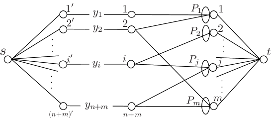
Figure 1: The polymatroidal network $\mathcal{N}$ in mechanism 1.

Each edge in $E$ is directed from $N$ to $M$. For each buyer $i$, consider copy $i^{\prime}$ and edge $i^{\prime}i$. The set of the copies of $X\subseteq N$ is denoted by $X^{\prime}$. Add source node $s$ and edge $si^{\prime}$ for each $i^{\prime}\in N^{\prime}$. Also, add sink node $t$ and edge $jt$ for each $j\in M$. Edge-capacity $c$ is defined from $y$ by

$$c(e):=\begin{cases}y_{i}\quad\,{\rm if}\ e=i^{\prime}i\ {\rm for}\ i\in N,\\ \infty\quad{\rm otherwise}.\end{cases}$$ (16)

Two polymatroids of each node are defined as follows. For $j\in M$, the polymatroid on $\delta^{-}_{j}=E_{j}$ is defined as $P_{j}$, and the other polymatroid on $\delta^{+}_{j}$ is defined by the capacity as in (10). Both two polymatroids of other nodes are defined by the capacity. Let $\mathcal{N}$ denote the resulting polymatroidal network.

Compute a maximum flow $\varphi$ in $\mathcal{N}$. The transaction vector $w$ of the original two-sided market is obtained as $w:=\varphi|_{E}$. By the construction, $w$ satisfies the polymatroid constraint. The payment vector $p$ is naturally given by $p:=\pi$, which satisfies the budget constraints. Also we choose $r$ as an arbitrary vector that satisfies

$$r_{j}-p_{n+j}+\rho_{j}y_{n+j} \geq\rho_{j}f_{j}(E_{j})\quad(j\in M),$$ (17)

$$\sum_{j\in M}r_{j} =\sum_{i\in N}p_{i}.$$ (18)

It turns out that the first condition (17) corresponds to (IRs), and the second condition (18) corresponds to (SBB).

Lemma 3.4.

There exists a vector $r$ satisfying $(\ref{irs_1})$ and $(\ref{budgetbalance_1})$.

We give in the next section a constructive proof of this lemma via mechanism 2.

After the procedure above, we obtain the allocation $(w,p,r)$ including virtual buyers. We transform this allocation into the allocation in the original market as follows:

• For each seller $j$, we regard $y_{n+j}=w_{(n+j)j}$ as the unsold goods of $j$, and replace the revenue $r_{j}$ by $r_{j}-p_{n+j}$.

By this update, (17) and (18) are equal to (IRs) and (SBB), respectively. Then we obtain the following theorem:

Theorem 3.5.

Mechanism 1 satisfies all the properties in Theorem 2.1.

Proof.

First we prove $w(E_{i})=y_{i}$ for each $i\in N$. Since $y$ is obtained by Algorithm 1, it holds $y\in\tilde{P}$ and thus there exists $\tilde{w}:=\{\tilde{w}_{ij}\}_{ij\in E}$ such that $\tilde{w}\in P$ and $\tilde{w}(E_{i})=y_{i}$. Then $\tilde{w}|_{E_{j}}\in P_{j}$ for each $j\in M$, and there exists a flow $\tilde{\varphi}$ such that $\tilde{\varphi}|_{E}=\tilde{w}$. By the flow-conservation law, it holds $\tilde{\varphi}({i^{\prime}i})=\tilde{w}(E_{i})=y_{i}$ for each $i\in N$. Since it holds $c(i^{\prime}i)=y_{i}$ for each $i\in N$, $\tilde{\varphi}$ is a maximum flow in $\mathcal{N}$. Therefore we obtain $\tilde{\varphi}({i^{\prime}i})=y_{i}$ for each $i\in N$ for any maximum flow $\tilde{\varphi}$ in $\mathcal{N}$. Thus the total amount of transaction of buyer $i$ is certainly $y_{i}$. By this fact and the definition of $p$, (ICb) and (IRb) are obtained immediately from Theorem 3.3.

As we mentioned, by the above update of the goods and revenue for sellers, (IRs) is equivalent to (17). Also (SBB) is nothing but (18).

The proof of (PO) is precisely the same as that for mechanism 2 (Theorem 3.11), which is given in Section 5. ∎

3.3 Second Mechanism

Next we describe mechanism 2, which is an extension of the polyhedral clinching auction to two-sided markets. First we make the same preprocessing as in mechanism 1 by adding virtual buyers.

After the preprocessing, we apply Algorithm 2, which is a two-sided version of the polyhedral clinching auction.

Algorithm 2 Polyhedral Clinching Auction for Two-Sided Market

1:  $p_{i}:=0,\ c_{i}:=0,\ d_{i}:=\infty\ (i\in N)\ {\rm and}\ l:=1$.

2:  $r_{j}:=0\ (j\in M)\ {\rm and}\ w_{ij}:=0\ (ij\in E)$.

3:  while $d_{i}\neq 0$ for some $i\in N$ do

4:     for $i=1,2,\ldots,n+m$ do

5:        Clinch a maximal increase $(\xi_{ij})_{ij\in E_{i}}$ not affecting other buyers.

6:        $w_{ij}:=w_{ij}+\xi_{ij}\quad(ij\in E_{i})$.

7:        $\displaystyle p_{i}:=p_{i}+c_{i}\xi(E_{i}).$

8:        $d_{i}:=\begin{cases}(B_{i}-p_{i})/c_{i}\quad{\rm if}\ c_{i}<v^{\prime}_{i},\\ 0\quad\qquad\qquad\ \ {\rm otherwise}.\end{cases}$

9:     end for

10:     $\displaystyle r_{j}:=r_{j}+\sum_{ij\in E_{j}}c_{i}\xi_{ij}\quad(j\in M).$

11:     $c_{l}:=c_{l}+\varepsilon$.

12:     $l:=l+1\ {\rm mod\ }m+n$.

13:     $d_{l}:=\begin{cases}(B_{l}-p_{l})/c_{l}\quad{\rm if}\ c_{l}<v^{\prime}_{l},\\ 0\quad\qquad\qquad\ \ {\rm otherwise}.\end{cases}$

14:  end while

The variables $c_{i},d_{i},l$ and the parameter $\varepsilon$ are the same as in Algorithm 1. Suppose that $\varepsilon$ satisfies Assumption 3.2. The meaning of variables $\xi_{ij},w_{ij},p_{i},r_{j}$ is explained as follows:

• $\xi_{ij}$ is the increase of transactions between buyer $i$ and seller $j$ in the current iteration.

• $w_{ij}$ is the total amount of transaction between buyer $i$ and seller $j$. Transaction vector $(w_{ij})_{ij\in E}$ must belong to the polymatroid $P$ (defined in (13)).

• $p_{i}$ is the payment of buyer $i$.

• $r_{j}$ is the revenue of seller $j$.

Algorithm 2 terminates when $d_{i}=0$ for all buyers $i$, and outputs $(w,p,r)$ at this moment. The allocation $(w,p,r)$ obtained by Algorithm 2 includes that for virtual buyers. Applying the same transformation as in mechanism 1, we obtain the allocation $(w,p,r)$ for the original market.

Again we explain the details of “not affecting other buyers” in line 5. For transaction vector $w$ and demand vector $d:=(d_{i})_{i\in N}$, define the remnant supply polytope $P_{w,d}$ by

$$P_{w,d}:=\{x\in\mathbb{R}^{E}_{+}\mid w+x\in P,\ x(E_{i})\leq d_{i}\ (i\in N)\}.$$ (19)

In addition, for $\xi:=(\xi_{ij})_{ij\in E_{i}}\in\mathbb{R}^{E_{i}}_{+}$, define the remnant supply polytope $P^{i}_{w,d}(\xi)$ of remaining buyers $N-i$ by

$$P^{i}_{w,d}(\xi):=\{u\in\mathbb{R}^{N-i}_{+}\mid\exists x\in P_{w,d},\ x|_{E_{i}}=\xi,\ x(E_{k})=u_{k}\ (k\in N-i)\}.$$ (20)

The first polytope $P_{w,d}\subseteq P$ represents the feasible increases of transactions under $w$ and $d$, and the second polytope $P^{i}_{w,d}(\xi)\subseteq\mathbb{R}^{N-i}_{+}$ represents the possible amounts of goods that buyers except $i$ can get in the future, provided $i$ got $\xi\in\mathbb{R}^{E_{i}}_{+}$ in this iteration. Then the condition for clinching $\xi:=(\xi_{ij})_{ij\in E_{i}}$ not to affect other buyers is naturally written as $P^{i}_{w,d}(\xi)=P^{i}_{w,d}(0)$. This motivates to define the polytope $P^{i}_{w,d}$ by

$$P^{i}_{w,d}:=\{\xi\in\mathbb{R}_{+}^{E_{i}}\mid P^{i}_{w,d}(\xi)=P^{i}_{w,d}(0)\},$$ (21)

which we call the clinching polytope of buyer $i$. A clinching vector $(\xi_{ij})_{ij\in E_{i}}$ in line 5 is chosen as a maximal vector in the clinching polytope $P_{w,d}^{i}$. The following theorem says that this clinching step can be done in polynomial time.

Theorem 3.6.

The clinching polytope $P^{i}_{w,d}$ is a polymatroid, and the value of the corresponding submodular function can be computed in polynomial time. In particular, by the greedy algorithm, a maximal vector of $P^{i}_{w,d}$ can be computed in polynomial time.

This implies that our mechanism is implementable in practice. The proof of Theorem 3.6 is given in Section 5.1.

We analyze mechanism 2. First we show (SBB) for our mechanism. In line 10 of Algorithm 2, the total payment of buyers (including virtual buyers) is directly given to sellers in each iteration. Also, in the transformation of the allocation, both the total payment and the total revenue are subtracted by the total payment of virtual buyers. Thus we have:

Lemma 3.7.

Mechanism 2 satisfies (SBB).

For the individual rationality of sellers (IRs), we will prove in Section 5.1 that each seller $j$ and nonvirtual buyer $i$ transact only when the price clock $c_{i}$ is at least valuation $\rho_{j}$ and virtual buyer $n+j$ vanishes, i.e., $d_{n+j}=0$. Consequently the goods of $j$ are sold at price at least $\rho_{j}$, and we obtain (IRs); see (4).

Proposition 3.8.

Mechanism 2 satisfies (IRs).

The proof is given in Section 5.1. Next we consider other properties (ICb),(IRb), and (PO) in Theorem 2.1. We utilize the following theorem on the relationship between mechanism 1 and mechanism 2.

Theorem 3.9.

Suppose that $\varepsilon$ is the same in both Algorithms. At the end of algorithm, $(y,\pi)$ in Algorithm 1 is equal to $((w(E_{i}))_{i\in N},p)$ in Algorithm 2.

The proof of Theorem 3.9 is given in Section 5.2. Therefore in mechanism 2, the utility of buyers is the same as that in the reduced one-sided market. By this fact and Theorem 3.3 we have:

Corollary 3.10.

Mechanism 2 satisfies (ICb) and (IRb).

We now show Lemma 3.4 in mechanism 1.

Proof of Lemma 3.4.

We verify that the revenue vector $r$ obtained by Algorithm 2 satisfies (17)(=(IRs)) and (18)(=(SBB)) for mechanism 1. By Theorem 3.9, the payment vectors of buyers in both algorithms are the same. Therefore (18) follows from Lemma 3.7. Also, by Theorem 3.9, the amounts of unsold goods, which are the amounts of goods obtained by virtual buyers, in both algorithms are the same. Hence (IRs) for mechanism 2 (Proposition 3.8) implies (17) = (IRs) for mechanism 1. ∎

Goel et al. [14] proved (PO) for Algorithm 1. We combine Theorem 3.4 with their proof method and careful considerations on utilities of sellers, and prove (PO) for mechanism 2:

Theorem 3.11.

Our mechanism satisfies (PO).

The proof is given in Section 5.3.

Remark 2 (Concave Budget Constraint).

Our model and mechanisms naturally incorporate concave budget constraints, i.e., utility $u_{i}$ of each buyer $i$ is given by

$$u_{i}(\mathcal{A}):=\begin{cases}\displaystyle v_{i}w(E_{i})-p_{i}\ \ \ {\rm if}\ p_{i}\leq\phi_{i}(w(E_{i})),\\ -\infty\qquad\quad\qquad\ \ {\rm otherwise},\end{cases}$$

where $\phi_{i}:\mathbb{R}_{+}\to\mathbb{R}_{+}$ is a concave non-decreasing function with $\phi_{i}(0)=0$. In the case of the usual budget constraint, $\phi_{i}$ is defined by $\phi_{i}(0):=0$ and $\phi_{i}(x):=B_{i}$ for $x>0$. Concave budget constraint was considered by Goel et al. [13] for one-sided markets. They showed that the polyhedral clinching auction can be generalized to this setting. By using their idea, our mechanisms can also be adapted to have the same conclusion in Theorem 2.1.

The adaptation is given as follows. Each buyer reports the region $\{(p_{i},z_{i})\,|\,p_{i}\leq\phi_{i}(z_{i})\}$ to the auctioneer, and the budget feasibility is replaced by $p_{i}\leq\phi_{i}(w(E_{i}))$. Assume, as in Goel et al. [13], that the interval $\varepsilon$ of price clocks divides $\beta_{i}:=\lim_{x\to 0}\phi_{i}(x)/x$ for each $i$. The function $\phi_{i}$ for a virtual buyer $i\in N$ is defined by $\phi_{i}(z_{i}):=0$ if $z_{i}=0$ and $\infty$ otherwise. The demand $d_{i}$ is defined by

$$d_{i}:=\left\{\begin{array}[]{ll}\max\{z_{i}\mid\pi_{i}+c_{i}z_{i}\leq\phi_{i}(y_{i}+z_{i})\}&{\rm if}\ c_{i}<v^{\prime}_{i},\\ 0&{\rm otherwise}.\end{array}\right.$$

In mechanism 2, we use $w(E_{i})$ instead of $y_{i}$, and $p_{i}$ instead of $\pi_{i}$. In Section 5, we give every proof for the setting with concave budget constraints.

3.4 Example

Here we demonstrate the behavior of the mechanisms for a small two-sided market consisting of two buyers $1,2$ and two sellers $1,2$. Each seller $j$ has $s_{j}$ units of goods, and can transact with both buyers $1,2$ freely. Namely the market is represented as a complete bipartite graph $(N,M,E)$ with $N=\{1,2\}$, $M=\{1,2\}$ and $E=N\times M$, and the polymatroid constraint $P_{j}$ $(j=1,2)$ is given by the stock constraint $w_{1j}+w_{2j}\leq s_{j}$, $w_{1j}\geq 0$, and $w_{2j}\geq 0$; the corresponding submodular function $f_{j}$ is given by $f_{j}(F):=s_{j}$ if $F\neq\emptyset$ and $f_{j}(\emptyset):=0$. Suppose that buyer $i$ has budget $B_{i}$ and bid $v^{\prime}_{i}=v_{i}$, and seller $j$ has reserved price $\rho_{j}$.

The both mechanisms 1 and 2 first apply the preprocessing. Add virtual buyers $3,4$ to $N$, where $3$ and $4$ are adjacent only to sellers $1$ and $2$, respectively. Their bids and budgets are defined by $v_{3}:=\rho_{1}$, $v_{4}:=\rho_{2}$, and $B_{3}=B_{4}:=\infty$. According to (12), the polymatroid constraint $P_{j}$ $(j=1,2)$ is extended to

$$w_{1j}+w_{2j}+w_{(j+2)j}\leq s_{j},$$

$$w_{1j},w_{2j},w_{(j+2)j}\geq 0.$$

Then the whole polymatroid $P=P_{1}\oplus P_{2}$ is obtained by the union of these inequalities for $j=1,2$. See the left of Figure 2.

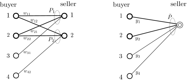
Figure 2: A two-sided market (left) and the reduced one-sided market (right)

We first consider mechanism 2. In some iteration of the mechanism, suppose that the transaction and demand vectors are given by $w$ and $d$, respectively. Let $\tilde{s}_{j}$ denote the current stock of the goods of seller $j$, i.e., $\tilde{s}_{j}:=s_{j}-w_{1j}-w_{2j}-w_{(j+2)j}$. Then the remnant supply polytope $P_{w,d}$ is given by

$$x_{1j}+x_{2j}+x_{(j+2)j}\leq\tilde{s}_{j}\quad(j=1,2),$$

$$x_{i1}+x_{i2}\leq d_{i}\quad(i=1,2),$$

$$x_{(j+2)j}\leq d_{j+2}\quad(j=1,2),$$

$$x_{ij}\geq 0\ (ij\in E).$$

We say that virtual buyer $j+2$ exists if $d_{j+2}=\infty$ and vanishes if $d_{j+2}=0$. For $j\in\{1,2\}$, let $e_{j}\in\{0,1\}$ be defined by $e_{j}:=1$ if $j+2$ exists and $e_{j}:=0$ otherwise. Also let $\bar{e}_{j}:=1-e_{j}$. For $i\in\{1,2\}$, let $i^{\prime}$ denote the companion of $i$, i.e., $\{1,2\}=\{i,i^{\prime}\}$. For nonvirtual buyer $i\in\{1,2\}$ and $\xi\in\mathbb{R}_{+}^{E_{i}}$, the remnant supply polytope $P^{i}_{w,d}(\xi)$ of remaining buyers $\{i^{\prime},3,4\}$ is given by

$$u_{i^{\prime}}+u_{3}+u_{4}\leq\tilde{s}_{1}+\tilde{s}_{2}-\xi_{i1}-\xi_{i2},$$

$$u_{i^{\prime}}\leq d_{i^{\prime}},\ u_{3}\leq(\tilde{s}_{1}-\xi_{i1})e_{1},\ u_{4}\leq(\tilde{s}_{2}-\xi_{i2})e_{2},$$

$$u_{i^{\prime}},u_{3},u_{4}\geq 0$$

if $\xi_{i1}+\xi_{i2}\leq d_{i}$, and $P^{i}_{w,d}(\xi)=\emptyset$ otherwise. For virtual buyer $j+2$ with $j\in\{1,2\}$ (if it exists) and $\xi=\xi_{(j+2)2}\geq 0$, the polytope $P^{j+2}_{w,d}(\xi)$ is given by

$$u_{1}+u_{2}+u_{j^{\prime}+2}\leq\tilde{s}_{1}+\tilde{s}_{2}-\xi_{(j+2)j},$$

$$u_{1}\leq d_{1},\ u_{2}\leq d_{2},\ u_{j^{\prime}+2}\leq\tilde{s}_{j^{\prime}}e_{j^{\prime}},$$

$$u_{1},u_{2},u_{j^{\prime}+2}\geq 0$$

if $\xi_{(j+2)j}\leq\tilde{s}_{j}$, and $P^{j+2}_{w,d}(\xi)=\emptyset$ otherwise. By elementary calculation, we can determine clinching polytopes $P_{w,d}^{i}$ $(i=1,2,3,4)$ as follows.

• For nonvirtual buyer $i\in\{1,2\}$, the clinching polytope $P^{i}_{w,d}$ is given by:

  $$\xi_{i1}+\xi_{i2}\leq\min\{d_{i},\max\{\tilde{s}_{1}\bar{e}_{1}+\tilde{s}_{2}\bar{e}_{2}-d_{i^{\prime}},0\}\},$$

  $$0\leq\xi_{i1}\leq\tilde{s}_{1}\bar{e}_{1},\ 0\leq\xi_{i2}\leq\tilde{s}_{2}\bar{e}_{2}.$$

• For virtual buyer $j+2$ with $j\in\{1,2\}$, the clinching polytope $P^{j+2}_{w,d}$ is given by

  $$0\leq\xi_{(j+2)j}\leq\max\{\tilde{s}_{j}+\tilde{s}_{j^{\prime}}\bar{e}_{j^{\prime}}-d_{1}-d_{2},0\}.$$

If virtual buyer $j+2$ exists, then any nonvirtual buyer cannot transact with $j$, i.e., $\xi_{ij}=0$, since this will interrupt $j+2$ who has infinite demand. After virtual buyers vanish, buyer $i$ can clinch surplus $\tilde{s}_{1}+\tilde{s}_{2}-d_{i^{\prime}}$ which exceeds the demand of the competitor $i^{\prime}$. Here maximal clinching vectors forms the segment between $(\min\{\tilde{s}_{1},c\},c-\min\{\tilde{s}_{1},c\})$ and $(c-\min\{\tilde{s}_{2},c\},\min\{\tilde{s}_{2},c\})$, where $c:=\min\{d_{i},\max\{\tilde{s}_{1}+\tilde{s}_{2}-d_{i^{\prime}},0\}\}$. The clinch by virtual buyer $j+2$ can be understood as taking back the goods of $j$ exceeding the limit that nonvirtual buyers can buy.

The auction proceeds as follows. In earlier iterations where a virtual buyer $j+2$ exists, nonvirtual buyers cannot purchase the good of $j$. Also virtual buyer $j+2$ may clinch to take back the goods of $j$ which is guaranteed to be unsold. The virtual buyer $j+2$ will vanish when the price clock $c_{j}$ reaches at the reserved price $\rho_{j}$ of $j$ ($=$ bid $v_{j+2}$ of $j+2$). Consequently the good of $j$ will be sold at price at least $\rho_{j}$. In this way, virtual buyers increase the prices of the goods to reserved prices, and take back the unsold goods, until their vanishing. After that, nonvirtual buyer $i$ clinches surplus $\tilde{s}_{1}+\tilde{s}_{2}-d_{i^{\prime}}$ exceeding the potential of competitor $i^{\prime}$. Thus the total sum of demands $d_{1}+d_{2}+d_{3}+d_{4}$ keeps at least the current stock $\tilde{s}_{1}+\tilde{s}_{2}$. Prices are increasing, and demands are decreasing. Finally all demands are zero, and the stocks are zero, i.e., all goods are sold. The auction terminates.

Table 1 shows the behavior of mechanism 2 for this market with setting $v_{1}=3$, $B_{1}=12$, $v_{2}=3$, $B_{2}=11$, $\rho_{1}=1$, $s_{1}=7$, $\rho_{2}=1$, and $s_{2}=8$.

Table 1: behavior of mechanism 2

	buyer 1				buyer 2				seller 1			seller 2
	$B_{1}=12$, $v_{1}=3$				$B_{2}=11$, $v_{2}=3$				$\rho_{1}=1$, $s_{1}=7$			$\rho_{2}=1$, $s_{2}=8$
$l$	$c_{1}$	$d_{1}$	$\xi_{11}$	$\xi_{12}$	$c_{2}$	$d_{2}$	$\xi_{21}$	$\xi_{22}$	$\tilde{s}_{1}$	$\varDelta r_{1}$	$c_{3}$	$\tilde{s}_{2}$	$\varDelta r_{2}$	$c_{4}$
$1$	$0$	$\infty$			0	$\infty$			$7$		0	$8$		0
$2$	$1$	$12$			0	$\infty$			$7$		0	$8$		0
$3$	$1$	$12$			1	$11$			$7$		0	$8$		0
$4$	$1$	$12$			1	$11$			$7$		1	$8$		0
$5$	$1$	$12,8$	$2$	$2$	1	$11$	$3/2$	$3/2$	$7,5$	$7/2$	1	$8,6$	$7/2$	1
$6$	$2$	$4$			1	$8$	$7/4$	$9/4$	$7/2$	$7/4$	1	$9/2$	$9/4$	1
$7$	$2$	$4,2$	$7/8$	$9/8$	2	$2$			$7/4,7/8$	$7/4$	1	$9/4,9/8$	$9/4$	1
$8$	$2$	$2$			2	$2$			$7/8$		2	$9/8$		1
$9$	$2$	$2$			2	$2$			$7/8$		2	$9/8$		2
$10$	$3$	$0$			2	$2$	$7/8$	$9/8$	$7/8$	$7/4$	2	$9/8$	$9/4$	2
	obtained goods: $6$				obtained goods: $9$				unsold goods: $0$			unsold goods: $0$
	payment: $8$				payment: $11$				revenue: $8.75$			revenue: $10.25$
	utility: $10$				utility: $16$				utility: $8.75$			utility: $10.25$

In the first four iterations, nonvirtual buyers cannot clinch (i.e., $\xi_{ij}=0$), since price clocks are less than reserved prices of sellers, i.e., virtual buyers exist. Also no taking back by virtual buyers occurs; hence clinching vectors $\xi_{31}$ and $\xi_{42}$ are omitted in the table. The first clinching occurs in the 5th iteration ($l=5$). The clinching polytope $P_{w,d}^{1}$ for buyer $1$ is given by $\xi_{11}+\xi_{12}\leq\min\{12,\max\{7+8-11,0\}\}=4$, $\xi_{12}\leq 8$, and $\xi_{12}\leq 7$. The maximal clinching vectors form the segment between $(4,0)$ and $(0,4)$. Here the midpoint $(2,2)$ is chosen as a clinching vector $(\xi_{11},\xi_{12})$; this midpoint clinching rule is used in the sequel. Buyer $1$ pays $2$ to both sellers $1$ and $2$. The demand $d_{1}$ of buyer $1$ is updated to $8$. The stocks of sellers $1$ and $2$ are updated to $5$ and $6$, respectively. The next is the turn of buyer $2$, who also clinches $(\xi_{21},\xi_{22})=(3/2,3/2)$. In this iteration, sellers $1$ and $2$ obtain revenues $\varDelta r_{1}=\varDelta r_{2}=7/2$. The auction proceeds in this way. The result is given in the bottom of the table.

Next we consider mechanism $1$. The reduced one-sided market is obtained as follows. See the right of Figure 2. The aggregated polymatroid $\tilde{P}$ is given by

$$y_{1}+y_{2}+y_{3}+y_{4}\leq s_{1}+s_{2},$$

$$y_{3}\leq s_{1},\ y_{4}\leq s_{2},$$

$$y_{1},y_{2},y_{3},y_{4}\geq 0.$$

Given a transaction $y$ and demand $d$, the remnant supply polytope $\tilde{P}_{y,d}$ is given by

$$z_{1}+z_{2}+z_{3}+z_{4}\leq s^{\prime},$$

$$z_{1}\leq d_{1},\ z_{2}\leq d_{2},\ z_{3}\leq s^{\prime}_{1}e_{1},\ z_{4}\leq s^{\prime}_{2}e_{2}$$

$$z_{1},z_{2},z_{3},z_{4}\geq 0,$$

where $s^{\prime}:=s_{1}+s_{2}-y_{1}-y_{2}-y_{3}-y_{4}$ and $s^{\prime}_{j}:=s_{j}-y_{j+2}$ for $j=1,2$. Via $\tilde{P}_{y,d}^{i}(\zeta)$, the maximum clinch $\zeta_{i}$ is computed as follows:

• $\zeta_{i}=\min\{d_{i},\max\{s^{\prime}-s^{\prime}_{1}e_{1}-s^{\prime}_{2}e_{2}-d_{i^{\prime}},0\}\}$ for $i=1,2$.

• $\zeta_{j+2}=\min\{s^{\prime}_{j},\max\{s^{\prime}-s^{\prime}_{j^{\prime}}e_{j^{\prime}}-d_{1}-d_{2},0\}\}$ for $j=1,2$.

Then the auction proceeds as follows. Buyer 1 obtains $4$ units of goods at $l=5$, and $2$ units at $l=7$. The total is $6$ and the payment is $8$. Buyer 2 obtains $3$ units at $l=5$, $4$ units at $l=6$, and $2$ units at $l=10$. No clinching by virtual buyers occur. For each buyer, the obtained goods and the payment are the same as that in mechanism 2, as Theorem 3.9 says. In fact, a stronger property holds: they are the same at each iteration, i.e., $\zeta_{i}=\xi_{i1}+\xi_{i2}$ holds. This property is generally true, which will be shown in Corollary 5.4 and Theorems 5.6 and 5.7. After the auction, transaction $(w_{ij})$ is recovered so that it satisfies $w_{11}+w_{12}=6$, $w_{21}+w_{22}=9$, $w_{11}+w_{21}=7$, and $w_{12}+w_{22}=8$. One example is $(w_{11},w_{12},w_{21},w_{22})=(3,3,5,4)$. The whole revenue of the market is $19$, which is distributed to sellers $1,2$ so as to satisfy (17) and (18), i.e., $r_{1}+r_{2}=19$, $r_{1}\geq 7$, and $r_{2}\geq 8$. One possible distribution is $(r_{1},r_{2})=(9,10)$, i.e., both sellers have net profit $2$.

4 Discussion

In this paper, we presented the first generic framework (model and mechanisms) for auctions in two-sided markets under budget constraints. We think that our framework will be a springboard toward algorithmic mechanism design on two-sided markets. Here we discuss issues of our framework, and raise future research directions.

Our model assumes, for avoiding the impossibility theorem, that all sellers are truthful. This results in that our framework has a strong priority on buyers. Indeed, as shown in Theorem 3.9, our mechanisms yield the same output for buyers as the original polyhedral clinching auction applied to the reduced one-sided market. From this point, our mechanisms are acceptable to the buyer side. Therefore our mechanisms should be discussed from the seller side. For sellers, we consider only the minimum requirement (IRs), and do not take into account which sellers should obtain more revenue than others. The total revenue can be much greater than the total sum of the guaranteed minimum revenues of sellers. Thus, how the surplus is shared to sellers is one of central issues.

Mechanism 1 aggregates sellers into one seller at first. This makes the auction simple but loses the correspondence between goods and sellers. In particular, when a buyer $i$ clinches an amount $\zeta_{i}$ of the goods at price $c_{i}$, the resulting revenue $c_{i}\zeta_{i}$ is not distributed at this moment. In the last recovery step, the total revenue is distributed to sellers so that only (IRs) and (SBB) are satisfied. This can cause some unfairness. In the example in Section 3.4, the revenue sharing $(r_{1},r_{2})=(7,12)$ or $(11,8)$ is possible, which is apparently unfair since the two sellers have almost the same characteristics.

Another type of unfairness occurs in the following extreme example. The market consists of two buyers $1,2$ and two sellers $1,2$, where both sellers have one unit of divisible goods ($s_{1}=s_{2}=1$) and zero reserved price ($\rho_{1}=\rho_{2}=0$). The buyer $1$ has budget $B_{1}=1$ and bid $v_{1}^{\prime}=2$, and wants the goods of both sellers, The buyer $2$ has infinite budget $B_{2}=\infty$ and bid $v_{2}^{\prime}=1$, and wants the goods of seller $2$ only. In particular the goods of seller $2$ are more competitive than that of $1$. The market is depicted in Figure 3.

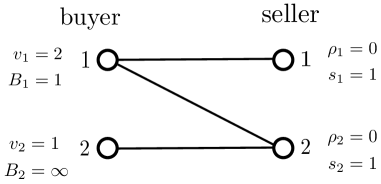
Figure 3: Seller 2 should obtain more revenue than seller 1.

Apply Algorithm 1 with $\varepsilon=1$; no virtual buyer exists by $\rho_{1}=\rho_{2}=0$. At the first iteration, buyer 1 clinches $1$ unit at price $0$, and also clinches $1$ unit at price $1$ when buyer 2 drops out from the auction, i.e., the price clock of buyer 2 reaches his bid. Then all the goods are sold. By (17) and (18), the revenue is distributed arbitrarily so that it satisfies $r_{1}\geq 0$, $r_{2}\geq 0$, $r_{1}+r_{2}=1$. In particular, $(r_{1},r_{2})=(1,0)$ can be chosen. However this revenue sharing opposes to our intuition that sellers who sold competitive goods should gain more revenue. Seller $2$ obtains no revenue, though his goods are competitive; it is wanted by both buyers. On the other hand, seller $1$ obtains revenue $1$ but his goods were sold by buyer 1 without competition. This example suggests that we should consider further constraints in the last recovery step so that the resulting sharing is “fair.” However we found it rather difficult to formalize the fairness mathematically. Such a concept should be defined only from the available information at this step, e.g., network structure $(N,M,E)$ and the recovered transaction $w$ (possibly not unique). This is a highly nontrivial problem, and should be left to future work.

Mechanism 2 is free from this annoying revenue sharing procedure. Indeed, actual transactions, prices, and revenues are opened and dynamically determined through iterations of the auction. Contrary to mechanism 1, the revenue obtained in each clinching is shared at this moment. Clearly sellers who sold their goods in high prices obtain more revenue. This is reasonable for all players in the auction. Also we think that mechanism 2 takes into account the competitiveness of goods by the following reason. Suppose that a buyer has a link to a competitive seller. Then the transaction on this link is influential to others, and hence it is hard for the buyer to clinch a large amount of the goods through this link. This consequently makes competitive goods sold in high prices, since the price increases through the auction. If mechanism 2 is applied to the above example, the resulting revenue of sellers is $(r_{1},r_{2})=(0,1)$, which is consistent with our intuition. From this point, we can say that mechanism 2 is superior to mechanism 1.

The main issue of mechanism 2 is the choice of maximal clinching vectors and its affect on the revenue of sellers. The clinching polytope is a polymatroid, and a maximal clinching vector is efficiently obtained (Theorem 3.6) but it is not unique in general. The choice of a maximal clinching vector is directly related to the revenues of sellers. Indeed, nontrivial clinching occurs after virtual buyers vanish, and the prices are monotonically increasing in the auction. This means that sellers obtain more revenue if his goods are sold in latter iterations. In the example of Section 3.4, we used the midpoint point clinching rule. We can change the clinching rule as: (i) each buyer $i$ chooses the clinching vector with the maximum $\xi_{i1}$ and (ii) each buyer $i$ chooses the clinching vector with the maximum $\xi_{i2}$. Then the revenue vector $(r_{1},r_{2})$ changes from $(8.75,10.25)$ to $(7,12)$ for (i) and to $(11,8)$ for (ii). Namely, by the choice of clinching vectors, mechanism 2 can yield the unfair revenue sharing $(7,12)$ and $(11,8)$.

Therefore we should consider a “fair” rule of choosing a maximal clinching vector. One practically reasonable way is to choose a random ordering of sellers (linked to a buyer doing clinch) and to run the greedy algorithm according to the ordering. Another natural way is to choose a kind of “center” in the polytope (base polytope) of maximal vectors of the clinching polytope. Natural candidates are the Shapley vector and a vector obtained by solving the resource allocation problem with an appropriate objective function. The former is NP-hard to be computed, and the latter is efficiently obtained via nonlinear optimization technique over polymatroids [10, Chapter V]. However we do not know any theoretical guarantee for these ways of clinching, even we did not formulate appropriate mathematical concepts (beyond (IRs)) that represent the fairness for sellers and that should be guaranteed.

Formalizing such a fairness concept may be an unavoidable theme for two-sided models. One possible approach is the $\alpha$-envy freeness introduced by Goel et al. [11], which is explained as follows. In the usual situation of auction, each seller $j$ obtains revenue via buying events involving $j$. Here let ${\cal E}_{j}$ denote the set of buying events involving $j$. Then the revenue sharing of a mechanism is said to be $\alpha$-envy-free $(\alpha\leq 1)$ if for any pair of sellers $j,j^{\prime}$, the revenue of $j$ (obtained at ${\cal E}_{j}$) is at least $\alpha$ times the (scaled) revenue of $j^{\prime}$ obtained at ${\cal E}_{j^{\prime}}\cap{\cal E}_{j}$. The $1$-envy free situation achieves an ideal fair sharing in the sense that every seller $j$ does not envy any other seller for his revenue obtained in events that $j$ participates. In mechanism 2, a buying event is precisely the clinch of some buyer $i$ at some iteration $l$. Namely ${\cal E}_{j}$ is the set of all pairs $(i,l)$ of buyers $i\in E_{j}$ and positive integers $l$. Let $r_{j}(i,l)$ denote the revenue of seller $i$ obtained at the clinch of buyer $i$ in iteration $l$. Then the $\alpha$-envy freeness in mechanism 2 can be formulated: For any pair of sellers $j,j^{\prime}$, it holds

$$r_{j}=\sum_{(i,l)\in{\cal E}_{j}}r_{j}(i,l)\geq\alpha\min\left(1,\frac{f_{j}(E_{j})}{f_{j^{\prime}}(E_{j^{\prime},j})}\right)\sum_{(i,l)\in{\cal E}_{j}\cap{\cal E}_{j^{\prime}}}r_{j^{\prime}}(i,l),$$

where $E_{j^{\prime},j}\subseteq E_{j^{\prime}}$ denote the set of edges in $E_{j^{\prime}}$ incident to buyers transacting with $j$, and $\min(1,f_{j}(E_{j})/f_{j^{\prime}}(E_{j^{\prime},j}))$ means a scaling factor adjusting the difference of supplies of $j,j^{\prime}$ (viewed from $j$). For the instance in Section 3.4, the midpoint clinching rule gives $0.896$-envy free sharing, whereas the rules (i) and (ii) give $0.666$- and $0.727$-envy free sharing, respectively. It fits our intuition that the midpoint rule is fair. A further analysis of our mechanism 2 and developing fair clinching rules by means of the envy-freeness deserve interesting future research.

Finally we mention some of remaining issues and future research directions.

• Our mechanisms terminate when all buyers have no demand. The required number of iterations is obviously bounded by $\sum_{i\in N}\lceil v^{\prime}_{i}/\varepsilon\rceil$. In the computational complexity point of view, our mechanisms are not polynomial time algorithms, though each iteration can be done in polynomial time (Theorem 3.6). This is already the case for one-sided clinching-type mechanisms [5, 14]. Acceleration of these mechanisms has not been studied so far. It would be interesting to improve clinching-type mechanisms to terminate in polynomial number of iterations.

• In this paper, we dealt with divisible goods. We do not know whether our framework and results can be extended to auctions with indivisible goods. Even if each $f_{j}\ (j\in M)$ is integer-valued, $f_{w,d}$ is not necessarily integer-valued. This prevents our mechanisms from dealing with indivisible goods. Notice that this is already the case for the original polyhedral clinching auction. To extend our framework for indivisible goods, the following work may be instrumental: Fiat et al. [8] presented a mechanism enjoying (IC), (IR), and (PO) for one-sided markets, where the seller has several kinds of goods and one indivisible unit for each goods. Colini-Baldeschi et al. [4] extended it to the multiple unit case. Goel et al. [11] addressed two-sided markets with indivisible goods and presented a clinching-type mechanism, though buyers are non-budgeted.

• It would be interesting to study further generalizations of our framework. For example, suppose that each buyer has a preference on sellers. In this situation, our mechanism 2 can naturally incorporate the preference. Indeed, each buyer can clinch a maximal vector according to the greedy algorithm using the ordering of his preference. Adding polymatroid constraints to both buyers and sellers is also a natural generalization to which the polymatroidal-flow approach could be applicable. Although extending polymatroid constraints to general polyhedral constraints can cause an impossibility theorem (already for one-sided markets) [14], several nice classes of polyhedra generalizing polymatroids are known in the literature of combinatorial optimization. Bisubmodular polyhedra are such a generalization of polymatroids; see [10, Section 3.5]. This polyhedron shares several nice common features with polymatroid, such as greedy algorithm and several polynomial-time operations. It may be interesting to explore the power of bisubmodular polyhedra for the design of auctions and mechanisms.

5 Proofs

In this section, we give proofs of claimed results in Section 3. In the market $(N,M,E)$, for node subset $Z$, let $E_{Z}$ denote the set of edges incident to nodes in $Z$. For edge subset $F$, let $N_{F}$ denote the set of buyers incident to $F$.

5.1 Proof of Theorem 3.6 and Proposition 3.8

Let $d$ be the demand vector, and $w$ the transaction vector in line 4 in the current iteration. We start to study polytopes $P_{w,d}$, $P_{w,d}^{i}(\xi)$, and $P_{w,d}^{i}$ from the viewpoint of polymatroidal network flow. For each seller $j$, define polytope $P_{j,w}\subseteq\mathbb{R}_{+}^{E_{j}}$ by

$$P_{j,w}:=\{x\in\mathbb{R}_{+}^{E_{j}}\mid w|_{E_{j}}+x\in P_{j}\}.$$

Since $P_{j,w}$ is a contraction of $P_{j}$ (see; e.g. Fujishige [10, Section 3.1]), $P_{j,w}$ is a polymatroid, and the corresponding submodular function $f_{j,w}:2^{E_{j}}\to\mathbb{R}_{+}$ is given by

$$f_{j,w}(F):=\min_{F^{\prime}\supseteq F}\{f_{j}(F^{\prime})-w(F^{\prime})\}\quad(F\subseteq E_{j}).$$

This fact is also observed from (i) $x(F^{\prime})\leq f_{j}(F^{\prime})-w(F^{\prime})$ implies $x(F)\leq f_{j}(F^{\prime})-w(F^{\prime})$ for $F\subseteq F^{\prime}$ by the nonnegativity of $x$, (ii) $f_{j}(F^{\prime})-w(F^{\prime})\geq 0$ since $w$ is a feasible transaction, and (iii) if $f_{j,w}(F)=f_{j}(F^{\prime})-w(F^{\prime})$ and $f_{j,w}(G)=f_{j}(G^{\prime})-w(G^{\prime})$, then

$$f_{j,w}(F)+f_{j,w}(G)$$

$$=f_{j}(F^{\prime})-w(F^{\prime})+f_{j}(G^{\prime})-w(G^{\prime})$$

$$\geq f_{j}(F^{\prime}\cap G^{\prime})-w(F^{\prime}\cap G^{\prime})+f_{j}(F^{\prime}\cup G^{\prime})-w(F^{\prime}\cup G^{\prime})$$

$$\geq f_{j,w}(F\cap G)+f_{j,w}(F\cup G).$$ (22)

We also define $f,f_{w}:2^{E}\to\mathbb{R}_{+}$ by

$$f(F) :=\sum_{j\in M}f_{j}(E_{j}\cap F)\quad(F\subseteq E),$$

$$f_{w}(F) :=\min_{F^{\prime}\supseteq F}\{f(F^{\prime})-w(F^{\prime})\}=\sum_{j\in M}f_{j,w}(E_{j}\cap F)\quad(F\subseteq E).$$

Note that both $f$ and $f_{w}$ are monotone submodular. In particular, $f$ corresponds to the polymatroid $P$ (by a theorem in McDiarmid [18]).

Let us construct a polymatroidal network from the market $(N,M,E)$, demand $d$, and polymatroids $P_{j,w}$ for each $j\in M$; see Figure 4.

Figure 4: The polymatroidal network $\mathcal{N}$

Each edge in $E$ is directed from $N$ to $M$. For each buyer $i$, consider copy $i^{\prime}$ of $i$ and (directed) edge $i^{\prime}i$. The set of the copies of $X\subseteq N$ is denoted by $X^{\prime}$. Add source node $s$ and edge $si^{\prime}$ for each $i^{\prime}\in N^{\prime}$. Also, add sink node $t$ and edge $jt$ for each $j\in M$. Edge-capacity $c$ is defined by

$$c(e):=\begin{cases}d_{i}\quad\,{\rm if}\ e=i^{\prime}i\ {\rm for}\ i\in N,\\ \infty\quad{\rm otherwise}.\end{cases}$$ (23)

Two polymatroids of each node are defined as follows. For $j\in M$, the polymatroid on $\delta^{-}_{j}=E_{j}$ is defined as $P_{j,w}$, and the other polymatroid on $\delta^{+}_{j}$ is defined by the capacity (23) as in (10). Two polymatroids of other nodes are defined by the capacity. Let $\mathcal{N}$ denote the resulting polymatroidal network.

Now the remnant supply polytope $P_{w,d}$ is written by using flows in $\mathcal{N}$:

$$P_{w,d}=\{x\in\mathbb{R}_{+}^{E}\mid\exists\varphi:{\rm flow\ in}\ \mathcal{N},x=\varphi|_{E}\}.$$

In the proof, the following function $f_{w,d}:2^{E}\to\mathbb{R}_{+}$ plays a key role

$$f_{w,d}(F):=\max_{x\in P_{w,d}}x(F)=\max_{\varphi:\,{\rm flow}\,{\rm in}\,\mathcal{N}}\varphi(F)\quad(F\subseteq E).$$ (24)

Then we obtain the following:

Theorem 5.1.

For $F\subseteq E$, it holds

$$f_{w,d}(F)=\min_{X\subseteq N_{F}}\{f_{w}(E_{X}\cap F)+d(N_{F}\setminus X)\},$$ (25)

and $f_{w,d}(F)$ can be computed in polynomial time, provided the value oracle of each $f_{j}$ is available.

Proof.

We modify $\mathcal{N}$ so that $f_{w,d}(F)$ is equal to the maximum flow value. Change the capacity of each $e\in E\setminus F$ to $0$. Also, for each $i\in N\setminus N_{F}$, change $c(i^{\prime}i)$ to $0$. Then the maximum flow value is equal to $f_{w,d}(F)$. By Theorem 3.1, the value $f_{w,d}(F)$ is equal to (11). Observe that subset $U$ attaining the minimum can take a form of $(N^{\prime}\cup X)+s$ for $X\subseteq N_{F}$. Then the set $\delta^{+}_{U}$ of edges leaving $U$ is equal to $\{i^{\prime}i\mid i\in N_{F}\setminus X\}\cup E_{X}$. In a partition $\{A,B\}$ of $\delta^{+}_{U}$ attaining minimum, edge $i^{\prime}i$ contributes $d_{i}$ in both cases of $i^{\prime}i\in A$ and $i^{\prime}i\in B$. Each edge $e$ in $E_{X}\cap F$ must be in $A$ (by $c(e)=\infty$), and each edge $e$ in $E_{X}\setminus F$ can be in $B$ (by $c(e)=0$ and monotonicity of $f_{w}$). Thus we have (25).

In the modified network ${\cal N}$, $f_{w,d}(F)$ can be computed by solving a maximum polymatroidal flow problem. There are several polynomial time algorithms for this problem; see Fujishige [10, Section 5.5]. ∎

Let $\xi\in\mathbb{R}^{E_{i}}_{+}$. We consider the remnant supply polytope $P^{i}_{w,d}(\xi)$ of remaining buyers except $i$ and the clinching polytope $P^{i}_{w,d}$ of $i$; see (20) and (21) for definition. Define $h^{i}_{\xi}:2^{N-i}\to\mathbb{R}_{+}$ and $h_{w,d}^{i}:2^{E_{i}}\to\mathbb{R}_{+}$ by

$$h^{i}_{\xi}(Y) :=\min_{F\subseteq E_{i}}\{f_{w,d}(E_{Y}\cup F)-\xi(F)\}\quad(Y\subseteq N-i),$$ (26)

$$h_{w,d}^{i}(F) :=f_{w,d}(E_{N-i}\cup F)-f_{w,d}(E_{N-i})\quad(F\subseteq E_{i}).$$

Our goal is to show the following:

Theorem 5.2.

• $P^{i}_{w,d}(\xi)$ is nonempty if and only if $h^{i}_{\xi}$ is nonnegative valued; in this case, $h^{i}_{\xi}$ is monotone submodular on $N-i$, and $P^{i}_{w,d}(\xi)$ coincides with the polymatroid associated with $h^{i}_{\xi}$.

• $h_{w,d}^{i}$ is monotone submodular on $E_{i}$, and $P^{i}_{w,d}$ coincides with the polymatroid associated with $h_{w,d}^{i}$.

Theorem 3.6 is an immediate consequence of Theorems 5.1 and 5.2 (ii).

Proof.

(i). We utilize the polymatroidal network $\mathcal{N}$. Then $u\in P_{w,d}^{i}(\xi)$ if and only if there exists a flow $\varphi$ in $\mathcal{N}$ such that $\varphi(ij)=\xi_{ij}$ for $ij\in E_{i}$, $\varphi(i^{\prime}i)=\xi(E_{i})\leq d_{i}$, and $\varphi(sk^{\prime})=u_{k}$ for $k\in N-i$. By modifying $\mathcal{N}$, we give an equivalent condition as follows. Replace $ij\in E_{i}$ by $sj$ with capacity $\xi_{ij}$, change capacity $c(sk^{\prime})$ of $sk^{\prime}$ to $u_{k}$ for $k\in N-i$, and delete nodes $i^{\prime}$ and $i$. By $\xi(E_{i})\leq d_{i}$ and Theorem 3.1, the above condition for $u\in P_{w,d}^{i}(\xi)$ can be written as:

• The maximum flow value is equal to $\xi(E_{i})+u(N-i)$, or equivalently, $U=\{s\}$ and $(A,B)=(\emptyset,\delta^{+}_{s})$ attain the minimum of (11).

In the minimum of (11), it suffices to consider $U$ of form $U=(Y^{\prime}\cup Z)+s$ for $Z\subseteq Y\subseteq N-i$. (If $k\in U\not\ni k^{\prime}$, then we can remove $k$ from $U$ without increasing the cut value.) Then the set $\delta^{+}_{U}$ of edges leaving $U$ is equal to $E_{i}\cup\{sk^{\prime}\mid k\in N\setminus(Y+i)\}\cup\{k^{\prime}k\mid k\in Y\setminus Z\}\cup E_{Z}$. In any partition $\{A,B\}$ of $\delta^{+}_{U}$, edge $sk^{\prime}$ contributes $u_{k}$, and $k^{\prime}k$ contributes $d_{k}$. It must hold $E_{Z}\subseteq A$. Thus it suffices to consider a partition $\{F,E_{i}\setminus F\}$ of $E_{i}$. Then $u\in P^{i}_{w,d}(\xi)$ if and only if

$$\xi(E_{i})+u(N-i)\leq f_{w}(E_{Z}\cup F)+\xi(E_{i}\setminus F)+u((N-i)\setminus Y)+d(Y\setminus Z)$$

for $F\subseteq E_{i}$ and $Z\subseteq Y\subseteq N-i$. This is further equivalent to

$$u(Y)\leq\min_{Z\subseteq Y,F\subseteq E_{i}}\{f_{w}(E_{Z}\cup F)+d(Y\setminus Z)-\xi(F)\}\quad(Y\subseteq N-i).$$ (27)

In particular, $P^{i}_{w,d}(\xi)$ is nonempty if and only if the right hand side of (27) is nonnegative. Define $\tilde{h}^{i}_{\xi}:2^{N-i}\to\mathbb{R}_{+}$ by the right hand side of (27). It suffices to show that $\tilde{h}^{i}_{\xi}$ is equal to $h^{i}_{\xi}$, and is monotone submodular if it is nonnegative valued.

We first show $h^{i}_{\xi}(Y)=\tilde{h}^{i}_{\xi}(Y)$ for $Y\subseteq N-i$. By substituting the formula (25) of $f_{w,d}$ for the definition (26) of $h^{i}_{\xi}$, we obtain

$$h^{i}_{\xi}(Y) =\min_{F\subseteq E_{i}}\{\min_{Z^{\prime}\subseteq N_{E_{Y}\cup F}}\{f_{w}(E_{Z^{\prime}}\cap(E_{Y}\cup F))+d(N_{E_{Y}\cup F}\setminus Z^{\prime})\}-\xi(F)\}.$$ (28)

Observe that

$$N_{E_{Y}\cup F}=\left\{\begin{array}[]{cc}Y+i&{\rm if}\ F\neq\emptyset,\\ Y&{\rm if}\ F=\emptyset.\end{array}\right.$$

Therefore the minimum in (28) is taken over $(F,Z^{\prime})$ with $\emptyset\neq F\subseteq E_{i}$, $Z^{\prime}\subseteq Y+i$ and over $(F,Z^{\prime})$ with $F=\emptyset$, $Z^{\prime}\subseteq Y$. Notice that if $F=\emptyset$, then $Z^{\prime}$ and $Z^{\prime}-i$ have the same value in (28). Thus $h^{i}_{\xi}$ is also written as

$$h^{i}_{\xi}(Y) =\min_{Z^{\prime}\subseteq Y+i,\ F\subseteq E_{i}}\{f_{w}(E_{Z^{\prime}}\cap(E_{Y}\cup F))+d(N_{E_{Y}\cup F}\setminus Z^{\prime})-\xi(F)\}.$$ (29)

We consider the minimum of (29) over all $Z^{\prime}\subseteq Y$ and over all $Z^{\prime}=Z+i$ with $Z\subseteq Y$. The first minimum $\alpha$ is equal to

$$\min_{Z^{\prime}\subseteq Y,\ F\subseteq E_{i}}\{f_{w}(E_{Z^{\prime}})+d(N_{E_{Y}\cup F}\setminus Z^{\prime})-\xi(F)\}$$

$$=\min_{Z^{\prime}\subseteq Y,\ F\subseteq E_{i}}\{f_{w}(E_{Z^{\prime}})+d(Y\setminus Z^{\prime})+d(N_{F})-\xi(F)\}$$

$$=\min_{Z^{\prime}\subseteq Y}\{f_{w}(E_{Z^{\prime}})+d(Y\setminus Z^{\prime})\},$$

where $F=\emptyset$ attains the minimum since $d_{i}\geq\xi(F)$. The second minimum $\beta$ is equal to

$$\min_{Z\subseteq Y,\ F\subseteq E_{i}}\{f_{w}(E_{Z+i}\cap(E_{Y}\cup F))+d(N_{E_{Y}\cup F}\setminus(Z+i))-\xi(F)\}$$

$$=\min_{Z\subseteq Y,\ F\subseteq E_{i}}\{f_{w}(E_{Z}\cup F)+d(Y\setminus Z)-\xi(F)\}$$

$$=\tilde{h}^{i}_{\xi}(Y)$$

Observe that $\alpha\geq\beta$ (since the first is the special case of $F=\emptyset$ in the second). Thus $h^{i}_{\xi}(Y)=\min\{\alpha,\beta\}=\beta=\tilde{h}^{i}_{\xi}(Y)$ as required.

Suppose that $\tilde{h}^{i}_{\xi}$ is nonnegative valued. Here $\tilde{h}^{i}_{\xi}(Y)$ is interpreted as the maximum value of a flow from $Y^{\prime}$ to $t$ in ${\cal N}$ with the transaction $w$ replaced by $w+\xi$, where $\xi$ is extended as $\xi:E\to\mathbb{R}_{+}$ by $\xi(e):=0$ for $e\in E\setminus E_{i}$. Note that $w+\xi$ is actually a feasible transaction by $f(F)-(w+\xi)(F)\geq f_{w}(F)-\xi(F)\geq 0$, where the last inequality follows from the nonnegativity of (27) (with $Y=\emptyset$). Via Theorem 5.1, the maximum flow value is equal to $\min_{Z\subseteq Y}\{f_{w+\xi}(E_{Z})+d(Y\setminus Z)\}$. Then, substitute $f_{w+\xi}(E_{Z})=\min_{H\supseteq E_{Z}}\{f(H)-w(H)-\xi(H)\}=\min_{H\supseteq H^{\prime}\supseteq E_{Z}}\{f(H)-w(H)-\xi(H^{\prime})\}=\min_{H^{\prime}\supseteq E_{Z}}\{f_{w}(H^{\prime})-\xi(H^{\prime})\}=\min_{F\subseteq E_{i}}\{f_{w}(E_{Z}\cup F)-\xi(F)\}$, where we use $\xi(H^{\prime})=\xi(E_{i}\cap H^{\prime})$ and the monotonicity of $f_{w}$. Namely $\tilde{h}^{i}_{\xi}$ is viewed as a network induction of $f_{w}$ [18], and is necessarily monotone submodular; one can also see the submodularity directly by taking minimizers of $\tilde{h}^{i}_{\xi}(X)$ and $\tilde{h}^{i}_{\xi}(Y)$ (as in (22))

(ii). By (i), we have $P^{i}_{w,d}(\xi)=P^{i}_{w,d}(0)$ if and only if $h^{i}_{\xi}(X)=h^{i}_{0}(X)$ for each $X\subseteq N-i$. By the monotonicity of $f_{w,d}$, the latter condition is equivalent to

$$(h_{\xi}^{i}(X):=)\min_{F\subseteq E_{i}}\{f_{w,d}(E_{X}\cup F)-\xi(F)\}=f_{w,d}(E_{X})(=h_{0}^{i}(X)\geq 0)\quad(X\subseteq N-i).$$

Notice that this condition also guarantees $P_{w,d}^{i}(\xi)\neq\emptyset$. Thus $\xi\in\mathbb{R}_{+}^{E_{i}}$ belongs to $P^{i}_{w,d}$ if and only if it holds

$$\xi(F) \leq f_{w,d}(E_{X}\cup F)-f_{w,d}(E_{X})$$ (30)

for each $F\subseteq E_{i}$ and $X\subseteq N-i$. The latter condition is equivalent to

$$\xi(F) \leq\min_{X\subseteq N-i}\{f_{w,d}(E_{X}\cup F)-f_{w,d}(E_{X})\}$$

$$=\min_{X\subseteq N-i}\{f_{w,d}(E_{X+i}\setminus(E_{i}\setminus F))-f_{w,d}(E_{X}\setminus(E_{i}\setminus F))\}\quad(X\subseteq N-i),$$ (31)

where we use $E_{X}\cup F=E_{X+i}\setminus(E_{i}\setminus F)$ and $E_{X}=E_{X}\setminus(E_{i}\setminus F)$ for $X\subseteq N-i$. By Lemma 5.3 (i) shown below, the function

$$X\mapsto f_{w,d}(E_{X}\setminus(E_{i}\setminus F))=\\ \begin{cases}f_{w,d}(E_{X-i}\cup F)\quad\ {\rm if}\ i\in X,\\ f_{w,d}(E_{X})\qquad\qquad{\rm otherwise}\end{cases}$$

is monotone submodular on $N$. By (1), the minimum in (31) is attained by $X=N-i$. Thus we have

$$\xi(F) \leq f_{w,d}(E_{N}\setminus(E_{i}\setminus F))-f_{w,d}(E_{N-i}\setminus(E_{i}\setminus F))$$

$$=f_{w,d}(E_{N-i}\cup F)-f_{w,d}(E_{N-i})=h_{w,d}^{i}(F),$$

The monotone submodularity of $F\mapsto f_{w,d}(E_{N-i}\cup F)$ is shown in the next lemma (Lemma 5.3 (ii)). This concludes that the clinching polytope $P^{i}_{w,d}$ is the polymatroid associated with $h_{w,d}^{i}$, as required. ∎

Lemma 5.3.

• For $F\subseteq E_{i}$, the function $X\mapsto f_{w,d}(E_{X}\setminus(E_{i}\setminus F))$ is monotone submodular on $N$.

• For $X\subseteq N-i$, the function $G\mapsto f_{w,d}(E_{X}\cup G)-f_{w,d}(E_{X})$ is monotone submodular on $E_{i}$.

Note that $f_{w,d}$ is not necessarily submodular on $E$.

Proof.

The monotonicity of both functions in (i) and (ii) is immediate from the monotonicity of $f_{w,d}$ in (24). We show the submodularity.

(i) Let $G:=E_{i}\setminus F$. The submodularity of $X\mapsto f_{w,d}(E_{X}\setminus G)$ can directly be shown by using formula (25) and taking minimizers of $f_{w,d}(E_{X}\setminus G)$ and $f_{w,d}(E_{Y}\setminus G)$ (as in (22)). Instead, we consider a flow interpretation. Consider $\mathcal{N}$, and remove all edges in $G$. Then $f_{w,d}(E_{X}\setminus G)$ is equal to the maximum value of a flow from $X^{\prime}$ to $t$ in the network. Thus $X\to f_{w,d}(E_{X}\setminus G)$ is a network induction of $f_{w}$, and is submodular.

(ii) Let $F,G\subseteq E_{i}$. It suffices to consider the case where $F\not\subseteq G$ and $G\not\subseteq F$. In particular, both $F$ and $G$ are nonempty. Hence $N_{E_{X}\cup F}=N_{E_{X}\cup G}=X+i$. Consider minimizers $Y$ and $Z$, respectively, of $f_{w,d}(E_{X}\cup F)$ and $f_{w,d}(E_{X}\cup G)$ in (25). Namely $f_{w,d}(E_{X}\cup F)=f_{w}(E_{Y}\cap(E_{X}\cup F))+d((X+i)\setminus Y)$ and $f_{w,d}(E_{X}\cup G)=f_{w}(E_{Z}\cap(E_{X}\cup G))+d((X+i)\setminus Z)$. Here $Y,Z\subseteq X+i$.
Case 1: Both $Y$ and $Z$ contain $i$. Notice that $E_{Y}\cap(E_{X}\cup F)=E_{Y-i}\cup F$ and the same holds for $Z$. Then we have

$$f_{w,d}(E_{X}\cup F)+f_{w,d}(E_{X}\cup G)$$

$$\quad=f_{w}(E_{Y-i}\cup F)+d((X+i)\setminus Y)+f_{w}(E_{Z-i}\cup G)+d((X+i)\setminus Z)$$

$$\quad\geq f_{w}((E_{Y-i}\cup E_{Z-i})\cup(F\cup G))+d((X+i)\setminus(Y\cup Z))$$

$$\qquad+f_{w}((E_{Y-i}\cap E_{Z-i})\cup(F\cap G))+d((X+i)\setminus(Y\cap Z))$$

$$\quad=f_{w}(E_{(Y\cup Z)-i}\cup(F\cup G))+d((X+i)\setminus(Y\cup Z))$$

$$\qquad+f_{w}(E_{(Y\cap Z)-i}\cup(F\cap G))+d((X+i)\setminus(Y\cap Z))$$

$$\quad\geq f_{w,d}(E_{X}\cup(F\cup G))+f_{w,d}(E_{X}\cup(F\cap G)).$$

Case 2: At least one of $Y$ and $Z$ does not contain $i$, say $i\not\in Z$. By $X+i=N_{E_{X}\cup G}$, we have

$$f_{w,d}(E_{X}\cup G) =\min_{Z\subseteq X}\{f_{w}(E_{Z}\cap(E_{X}\cup G))+d((X+i)\setminus Z)\}$$

$$=\min_{Z\subseteq X}\{f_{w}(E_{Z})+d(X\setminus Z)+d_{i}\}=f_{w,d}(E_{X})+d_{i}.$$

Then we obtain

$$f_{w,d}(E_{X}\cup F)+f_{w,d}(E_{X}\cup G) =f_{w,d}(E_{X}\cup F)+f_{w,d}(E_{X})+d_{i}$$

$$\geq f_{w,d}(E_{X}\cup(F\cap G))+f_{w,d}(E_{X})+d_{i}$$

$$\geq f_{w,d}(E_{X}\cup(F\cap G))+f_{w,d}(E_{X}\cup(F\cup G)),$$

where the first inequality follows from the monotonicity of $f_{w,d}$ and the second inequality follows from $f_{w,d}(E_{X}\cup(F\cup G))\leq f_{w,d}(E_{X})+d_{i}$, i.e., the total flow on $E_{X}\cup(F\cup G)$ is at most the sum of the total flow on $E_{X}$ and capacity $d_{i}$ of $i^{\prime}i$. This concludes that $G\mapsto f_{w,d}(E_{X}\cup G)$ is submodular. ∎

By (30) in the proof of Theorem 5.2 (i) and Theorem 5.2 (ii), we obtain the following corollary.

Corollary 5.4.

Suppose that buyer $i$ clinches $\xi\in\mathbb{R}^{E_{i}}_{+}$ of goods.

• For $F\subseteq E_{i}$ and $X\subseteq N-i$, it holds $\xi(F)\leq f_{w,d}(E_{X}\cup F)-f_{w,d}(E_{X})$.

• Buyer $i$ gets $\xi(E_{i})=f_{w,d}(E)-f_{w,d}(E\setminus E_{i})$ amount of goods.

Next we prove Proposition 3.8 $=$ (IRs), which is an immediate consequence of the following.

Lemma 5.5.

For each seller $j$, if $c_{n+j}<\rho_{j}$, then $w_{ij}=0$ for all $ij\in E_{j}-(n+j)j$.

This means that the goods of each buyer $j$ are sold by nonvirtual buyer at price at least $\rho_{j}$. Therefore, after transforming the allocation of Algorithm 2 into the allocation without virtual buyers, it holds $r_{j}\geq\rho_{j}w(E_{j})$. Then we obtain (IRs): $u_{j}(\mathcal{M}(\mathcal{I}))=r_{j}+\rho_{j}(f_{j}(E_{j})-w(E_{j}))\geq\rho_{j}f_{j}(E_{j})$.

Proof.

It suffices to show that if $c_{n+j}<\rho_{j}$ and $w|_{E_{j}-(n+j)j}=0$ then $\xi|_{E_{j}-(n+j)j}=0$; consequently $w|_{E_{j}-(n+j)j}=0$ until $c_{n+j}=\rho_{j}$. By Corollary 5.4 (i) for $X=\{n+j\}$ and $F=\{ij\}$ with $i\neq n+j$, the clinching vector $\xi\in\mathbb{R}^{E_{i}}_{+}$ of buyer $i$ satisfies

$$\xi_{ij}\leq f_{w,d}(\{(n+j)j\}\cup\{ij\})-f_{w,d}(\{(n+j)j\}).$$

We show that the right hand side is zero. Now $d_{n+j}=\infty$ by $c_{n+j}<\rho_{j}$. Hence in the formula (25) of $f_{w,d}(\{(n+j)j\}\cup\{ij\})$, the minimum is attained by $X=\{n+j\}$ or $\{i,n+j\}$. Thus we have $f_{w,d}(\{(n+j)j\}\cup\{ij\})=\min\{f_{w}(\{(n+j)j\}\cup\{ij\}),f_{w}(\{(n+j)j\})+d_{i}\}$. Moreover we have

$$f_{w}(\{(n+j)j\}\cup\{ij\}) =f_{w,j}(\{(n+j)j\}\cup\{ij\})$$

$$=\min_{F\subseteq E_{j}:ij,(n+j)j\in F}f_{j}(F)-w(F)$$

$$=f_{j}(E_{j})-w_{(n+j)j},$$

where we use $w_{ij}=0$ for $ij\in E_{j}-(n+j)j$ and the modification (12) of $f_{j}$. Similarly $f_{w}(\{(n+j)j\})=f_{j}(E_{j})-w_{(n+j)j}$, and hence $f_{w,d}(\{(n+j)j\}\cup\{ij\})=f_{j}(E_{j})-w_{(n+j)j}$. Also $f_{w,d}(\{(n+j)j\})=f_{w}(\{(n+j)j\})=f_{j}(E_{j})-w_{(n+j)j}$. Thus we obtain $\xi_{ij}=0$. ∎

5.2 Proof of Theorem 3.9

Here we give a proof of Theorem 3.9. Consider the transaction vector $w\in\mathbb{R}_{+}^{E}$　 and demand vector $d\in\mathbb{R}_{+}^{N}$ in an iteration of Algorithm 2. Then feasible transaction $y:N\to\mathbb{R}_{+}$ for the reduced market is naturally given by $y_{i}:=w(E_{i})$ $(i\in N)$. We consider the behavior of Algorithm 1 for this $y,d$. It is known in [14] that $\tilde{P}$ is a polymatroid, and the corresponding submodular function $g$ is

$$g(X)=f(E_{X})\ \quad(X\subseteq N).$$

Also $\tilde{P}_{y,d}$ is a polymatroid, and the corresponding submodular function $g_{w,d}$ is given by

$$g_{w,d}(X) =\min_{Z\subseteq X}\{\min_{Z^{\prime}\supseteq Z}\{g(Z^{\prime})-w(E_{Z^{\prime}})\}+d(X\setminus Z)\}.$$

These facts are also obtained by considering the polymatroidal network with one seller (of polymatroid constraint $\tilde{P}$), as in Figure 4. The clinch $\zeta_{i}$ in Algorithm 1 is given as follows:

Theorem 5.6 (Goel et al. [14]).

In Algorithm 1, it holds $\zeta_{i}=g_{w,d}(N)-g_{w,d}(N-i)$ for each $i\in N$.

The goal of this section is to prove following:

Theorem 5.7.

In Algorithm 2, we have the following:

• $f_{w,d}(E_{X})=g_{w,d}(X)$ holds for each $X\subseteq N$.

• The value $f_{w,d}(E)-f_{w,d}(E\setminus E_{k})$ does not change after the clinch of buyer $i\in N-k$.

In particular, the total amount $\xi(E_{i})$ of the clinch of each buyer $i$ is determined by $w$ and $d$ at the beginning of For Loop in line 4 (i.e., independent of the ordering of buyers). Now $\epsilon$ is the same in both algorithms. By Corollary 5.4 (ii) and Theorems 5.6 and 5.7, we obtain Theorem 3.9 that in Algorithm 2 each buyer obtains the same total amount of goods as in Algorithm 1.

The rest of this subsection is devoted to proving Theorem 5.7. Define $\tilde{g}_{w,d}:2^{N}\to\mathbb{R}_{+}$ by

$$\tilde{g}_{w,d}(X):=f_{w,d}(E_{X})=\min_{Z\subseteq X}\{f_{w}(E_{Z})+d(X\setminus Z)\}\quad(X\subseteq N),$$ (32)

where we use (25) for the second equality. We first analyze the behavior of $\tilde{g}_{w,d}$ when buyer $i$ clinches. Suppose that $w$ and $d$ are the transaction vector and demand vector, respectively, at line 4 in the current iteration.

Lemma 5.8.

Suppose that buyer $i$ clinches $\xi\in\mathbb{R}^{E_{i}}_{+}$ of goods, and $w$ and $d$ are updated to $w^{\prime}$ and $d^{\prime}$, respectively, in lines 6–8. Then, for $X\subseteq N$, the following hold:

• If $i\in X$, then $\tilde{g}_{w^{\prime},d^{\prime}}(X)=\tilde{g}_{w,d}(X)-\xi(E_{i})$.

• If $i\not\in X$, then $\tilde{g}_{w^{\prime},d^{\prime}}(X)=\tilde{g}_{w,d}(X)$.

Now Theorem 5.7 (ii) is an immediate corollary of Lemma 5.8 (i) since

$$f_{w^{\prime},d^{\prime}}(E)-f_{w^{\prime},d^{\prime}}(E\setminus E_{k}) =\tilde{g}_{w^{\prime},d^{\prime}}(N)-\tilde{g}_{w^{\prime},d^{\prime}}(N-k)$$

$$=(\tilde{g}_{w,d}(N)-\xi(E_{i}))-(\tilde{g}_{w,d}(N-k)-\xi(E_{i}))$$

$$=f_{w,d}(E)-f_{w,d}(E\setminus E_{k}).$$ (33)

We prove (i) in the end, and we here only prove (ii).

Proof of Lemma 5.8 (ii).

Here $w^{\prime}(e)=w(e)$ for $e\in E\setminus E_{i}$ and $w^{\prime}(e)=w(e)+\xi(e)$ for $e\in E_{i}$, and $d^{\prime}_{k}=d_{k}$ for $k\neq i$. Then $\tilde{g}_{w^{\prime},d^{\prime}}(X)$ is given by

$$\tilde{g}_{w^{\prime},d^{\prime}}(X)=\min_{Z\subseteq X}\{f_{w^{\prime}}(E_{Z})+d(X\setminus Z)\}.$$ (34)

For $Z\subseteq X$, it holds

$$f_{w^{\prime}}(E_{Z})=\min_{G\subseteq E_{i}}\{f_{w}(E_{Z}\cup G)-\xi(G)\}$$

since $f_{w^{\prime}}(E_{Z})=\min_{H\supseteq E_{Z}}\{f(H)-w^{\prime}(H)\}=\min_{H\supseteq H^{\prime}\supseteq E_{Z}}\{f(H)-w(H)-\xi(H^{\prime}\cap E_{i})\}=\min_{H^{\prime}\supseteq E_{Z}}\{f_{w}(H^{\prime})-\xi(H^{\prime}\cap E_{i})\}=\min_{G\supseteq E_{i}}\{f_{w}(E_{Z}\cup G)-\xi(G)\}$; in the last equality put $G=H^{\prime}\cap E_{i}$ and use the monotonicity $f_{w}(H^{\prime})\geq f_{w}(E_{Z}\cup G)$. Then the inequality ($\leq$) follows from

$$\tilde{g}_{w^{\prime},d^{\prime}}(X) =\min_{Z\subseteq X}\{\min_{G\subseteq E_{i}}\{f_{w}(E_{Z}\cup G)-\xi(G)\}+d(X\setminus Z)\}$$

$$\leq\min_{Z\subseteq X}\{f_{w}(E_{Z})+d(X\setminus Z)\}=f_{w,d}(E_{X})=\tilde{g}_{w,d}(X).$$

($\geq$) follows from

$$\tilde{g}_{w^{\prime},d^{\prime}}(X) =\min_{Z\subseteq X}\{\min_{G\subseteq E_{i}}\{f_{w}(E_{Z}\cup G)-\xi(G)\}+d(X\setminus{Z})\}$$

$$=\min_{G\subseteq E_{i}}\{\min_{Z\subseteq X}\{f_{w}(E_{Z}\cup G)+d(X\setminus Z)\}-\xi(G)\}$$

$$\geq\min_{G\subseteq E_{i}}\{f_{w,d}(E_{X}\cup G)-\xi(G)\}$$

$$=f_{w,d}(E_{X})=\tilde{g}_{w,d}(X),$$

where the third equality follows from Corollary 5.4 (i), and the inequality can be verified from the definition (24) of $f_{w,d}(E_{X}\cup G)$. Namely the total flow on $E_{X}\cup G$ is at most the sum of the total flows on $E_{Z}\cup G$ and on $\{i^{\prime}i\mid i\in X\setminus Z\}$: the former is bounded by $f_{w}(E_{Z}\cup G)$ and the latter is bounded by $d(X\setminus Z)$. ∎

We next show Theorem 5.7 (i), i.e., $g_{w,d}(X)=\tilde{g}_{w,d}(X)(:=f_{w,d}(E_{X})$). Observe from the definitions that the two functions are written as:

$$g_{w,d}(X) =\min_{Z\subseteq X}\{\min_{Z^{\prime}\supseteq Z}\{f(E_{Z^{\prime}})-w(E_{Z^{\prime}})\}+d(X\setminus Z)\}.$$

$$\tilde{g}_{w,d}(X) =\min_{Z\subseteq X}\{\min_{F\supseteq E_{Z}}\{f(F)-w(F)\}+d(X\setminus Z)\}.$$

Comparing the inner minimums, we see that $g_{w,d}(X)\geq\tilde{g}_{w,d}(X)$ generally holds. We are going to show the converse. By a minimizer of $\tilde{g}_{w,d}(X)$ we mean a subset $Z\subseteq X$ satisfying $\tilde{g}_{w,d}(X)=\min_{F\supseteq E_{Z}}\{f(F)-w(F)\}+d(X\setminus Z)$. Our goal is to show that in Algorithm 2 there always exists a minimizer $Z$ of $\tilde{g}_{w,d}(X)$ such that $f(E_{Z})-w(E_{Z})=\min_{F\supseteq E_{Z}}\{f(F)-w(F)\}(=f_{w}(E_{Z}))$, which implies $g_{w,d}(X)=\tilde{g}_{w,d}(X)$.

Lemma 5.9.

For $X\subseteq N$, the following conditions are equivalent.

• $X$ is a (unique) minimal minimizer of $\tilde{g}_{w,d}(X)$; in this case, $\tilde{g}_{w,d}(X)=f_{w}(E_{X})$ holds.

• $X$ is a minimal minimizer of $\tilde{g}_{w,d}(Y)$ for some $Y$ with $X\subseteq Y\subseteq N$.

Proof.

It suffices to show that (ii) implies (i). Suppose that $X$ is a minimal minimizer of $\tilde{g}_{w,d}(Y)$ but $X$ is not a minimal minimizer of $\tilde{g}_{w,d}(X)$. Then there exists a proper subset $X^{\prime}\subset X$ such that $f_{w}(E_{X})\geq f_{w}(E_{X^{\prime}})+d(X\setminus X^{\prime})$. Then $f_{w}(E_{X})+d(Y\setminus X)\geq f_{w}(E_{X^{\prime}})+d(X\setminus X^{\prime})+d(Y\setminus X)=f_{w}(E_{X^{\prime}})+d(Y\setminus X^{\prime})$, which contradicts the minimality of $X$ for $\tilde{g}_{w,d}(Y)$. ∎

Let $\mathcal{U}\subseteq 2^{N}$ denote the family of subsets $X\subseteq N$ satisfying the conditions in Lemma 5.9. Namely, $X\in{\cal N}$ is a minimal minimizer of $\tilde{g}_{w,d}(Y)$ for some $Y$. By the argument before Lemma 5.9, the following (ii) completes the proof of Theorem 5.7 (i).

Proposition 5.10.

In Algorithm 2, the following hold:

• The family $\mathcal{U}$ is equal to $2^{N}$ at the beginning, and is monotone nonincreasing through the iterations.

• For each $X\in\mathcal{U}$, it always holds

  $$f_{w}(E_{X})=f(E_{X})-w(E_{X}).$$ (35)

Proof.

At beginning of the algorithm, it holds $w_{ij}=0\ (ij\in E)$ and $d_{i}=\infty\ (i\in N)$. Then ${\cal U}=2^{N}$. Also all $X$ satisfies (35) by the monotonicity of $f_{j}\ (j\in M)$.

Next we show: If $X\in{\cal U}$ satisfies (35) at line 4, then $X$ satisfies (35) in the For loop (line 4–8). Consider $X\in\mathcal{U}$ satisfying (35) at line 4 with the turn of buyer $i\in N$. Suppose that the buyer $i$ clinches $\xi\in\mathbb{R}^{E_{i}}_{+}$ of goods, and that $w,d$ are updated to $w^{\prime},d^{\prime}$ in lines 6–8. If $i\in X$, then for each $F\supseteq E_{X}$, $f(F)-w(F)$ decreases by $\xi(E_{i})$. Thus the equality (35) is keeping after lines 6–8. If $i\in N\setminus X$, then, by (35) for $w,d$ and Lemma 5.8 (ii), we have

$$\tilde{g}_{w^{\prime},d^{\prime}}(X)\leq f_{w^{\prime}}(E_{X})\leq f(E_{X})-w^{\prime}(E_{X})=f(E_{X})-w(E_{X})=f_{w}(E_{X})=\tilde{g}_{w,d}(X)=\tilde{g}_{w^{\prime},d^{\prime}}(X).$$

Thus we obtain (35) for new $w^{\prime},d^{\prime}$.

Next we show that no new sets are added to ${\cal U}$ in the For loop. (In fact, one can show that ${\cal U}$ does not change in the For loop.) Take $X\not\in{\cal U}$ at line 4. Then there is a minimal minimizer $Z\subset X$ of $\tilde{g}_{w,d}(X)$ such that

$$f_{w}(E_{X})\geq f_{w}(E_{Z})+d(X\setminus Z)=\tilde{g}_{w,d}(X).$$ (36)

Consider the clinch of buyer $i$ as above. If $X$ contains $i$, then both sides of (36) decrease by $\xi(E_{i})$, and $X$ is not a minimal minimizer for $\tilde{g}_{w^{\prime},d^{\prime}}(X)$. If $X$ does not contain $i$, then by (35) for $w,d$ and Lemma 5.8 (ii), we have $\tilde{g}_{w,d}(X)=f_{w}(Z)+d(X\setminus Z)=f(E_{Z})-w(E_{Z})+d(X\setminus Z)=f(E_{Z})-w^{\prime}(E_{Z})+d(X\setminus Z)\geq f_{w^{\prime}}(E_{Z})+d(X\setminus Z)\geq\tilde{g}_{w^{\prime},d^{\prime}}(X)=\tilde{g}_{w,d}(X)$, and this means that $Z\subset X$ is a minimizer of $\tilde{g}_{w^{\prime},d^{\prime}}(X)$. Hence $X\not\in{\cal U}$ holds after the clinch.

Finally we show that no sets are added to $\mathcal{U}$ by the calculation of $d_{l}$ in line 13. For each $X\notin\mathcal{U}$, there exists a proper subset $Z\subset X$ such that the inequality in (36) holds. Since $f_{w}$ does not depend on $d$, and $d$ is nonincreasing, this inequality still holds after the recalculation of $d_{l}$. Therefore it still holds that $X\notin\mathcal{U}$. ∎

Finally we prove Lemma 5.8 (i), which completes the proof of Theorem 5.7 (ii) by (33).

Proof of Lemma 5.8(i).

Consider $X\subseteq N$ with $i\in X$. Notice that $d_{i}$ is changed to $d^{\prime}_{i}=d_{i}-\xi(E_{i})$ after the clinch of $i$. Let $Z\in{\cal U}$ be a minimal minimizer of $\tilde{g}_{w,d}(X)$. By Proposition 5.10 (ii), we have $\tilde{g}_{w,d}(X)=f_{w}(E_{Z})+d(X\setminus Z)=f(E_{Z})-w(E_{Z})+d(X\setminus Z)$. After the clinch, the last quantity decreases by $\xi(E_{i})$ regardless whether $Z$ contains $i$ or not. This means that $\tilde{g}_{w^{\prime},d^{\prime}}(X)\leq\tilde{g}_{w,d}(X)-\xi(E_{i})$.

We show the converse. Let $Z^{\prime}\in{\cal U}$ be a minimal minimizer of $\tilde{g}_{w^{\prime},d^{\prime}}(X)$. By the monotonicity of ${\cal U}$ (Proposition 5.10 (i)), $Z^{\prime}$ belongs to ${\cal U}$ before the clinch. Therefore it holds again $\tilde{g}_{w,d}(X)\leq f_{w}(E_{Z^{\prime}})+d(X\setminus Z^{\prime})=f(E_{Z^{\prime}})-w(E_{Z^{\prime}})+d(X\setminus Z^{\prime})$. After the clinch, the last quantity decreases by $\xi(E_{i})$, which equals $\tilde{g}_{w^{\prime},d^{\prime}}(X)$. This means that $\tilde{g}_{w,d}(X)\leq\tilde{g}_{w^{\prime},d^{\prime}}(X)+\xi(E_{i})$. ∎

5.3 Proof of Theorem 3.11

Here we prove the pareto optimality (Theorem 3.11) in the setting of concave budget constraints (Remark 2). In the proof, it is important to analyze how buyers drop out of the auction, or situations when their demands become zero. Thanks to Theorem 3.9, we can use properties obtained in Goel et al. [13] for one-sided markets. We utilize the notion of the dropping price introduced by them. The dropping price of buyer $i$, denoted by $\theta_{i}$, is defined as the first price $c_{i}$ for which the demand $d_{i}$ is zero. As shown in [13], there are three cases when buyer $i$ drops out of the auction.

Case 1:

Buyer $i$ clinches his entire demand $\xi(E_{i})=d_{i}$. In this case, $\theta_{i}\leq v_{i}-\epsilon$. After the clinch, it holds $p_{i}=\phi_{i}(w(E_{i}))$. By the concavity of $\phi_{i}$, the demand never becomes positive.

Case 2:

Buyer $i$ does not clinch his entire demand but the price reaches his bid, i.e., $\theta_{i}=v_{i}^{\prime}$.

Case 3:

Buyer $i$ does not clinch his entire demand but $p_{i}=\beta_{i}w(E_{i})$ and $\theta_{i}>\beta_{i}$.

We here call the event of case 2 or 3 the unsaturated drop (of buyer $i$). Recall that $\beta_{i}:=\lim_{x\to+0}\phi_{i}(x)/x$ represents the angle of $\phi_{i}$ at $0$. In the usual budget constraints, case 1 means $p_{i}=B_{i}$ and case 3 never occurs (by $\beta_{i}=\infty$).

We use the following intriguing property to prove the pareto optimality (Theorem 3.11). Here a subset $X\subseteq N$ is said to be tight with respect to transaction $w$ if $w(E_{X})=f(E_{X})(=g(X))$.

Proposition 5.11 (Goel et al. [13]).

Let $i_{1},i_{2},\ldots,i_{t}$ be the buyers doing unsaturated drop, where they are sorted in reverse order of their drops; then $\theta_{i_{1}}\geq\cdots\geq\theta_{i_{t}}$. For each $k=1,2,\ldots,t$, let $X_{k}$ denote the set of buyers having a positive demand just before the drop of $i_{k}$. Then we have the following:

• $\emptyset=X_{0}\subset X_{1}\subset X_{2}\subset\cdots\subset X_{t}=N$ is a chain of tight sets.

• For $k=1,2,\ldots,t$, it holds $i_{k}\in X_{k}\setminus X_{k-1}$.

• For $i\in X_{k}\setminus(X_{k-1}+i_{k})$, it holds $\theta_{i}\in\{\theta_{i_{k}}-\varepsilon,\theta_{i_{k}}\}$.

The proof of PO in our mechanisms is a modification of that of [13, Theorem 4.6].

Proof of Theorem 3.11.

We denote the set of nonvirtual buyers by $N^{\ast}$. By (ICb) (Theorem 3.3 or Corollary 3.10), we may assume that each buyer $i$ reports true valuation, i.e., $v^{\prime}_{i}=v_{i}\ (i\in N^{\ast})$. Let $\mathcal{A}=(w,p,r)$ be the allocation obtained by Algorithm 2 (including the allocation to the virtual buyers). Consider an arbitrary allocation (without virtual buyers) $\mathcal{A}^{\prime}=(w^{\prime},p^{\prime},r^{\prime})$ such that

$$\sum_{i\in N^{\ast}}p^{\prime}_{i} \geq\sum_{j\in M}r^{\prime}_{j}$$ (37)

$$v_{i}w(E_{i})-p_{i} \leq v_{i}w^{\prime}(E_{i})-p^{\prime}_{i}\quad(i\in N^{\ast}),$$ (38)

$$(r_{j}-p_{n+j})+\rho_{j}w_{(n+j)j} \leq r^{\prime}_{j}+\rho_{j}(f_{j}(E_{j})-w^{\prime}(E_{j}))\quad(j\in M).$$ (39)

Our goal is to show that all inequalities in (38) and (39) hold in equality. Here $\mathcal{A}^{\prime}$ is extended to an allocation with virtual buyers by:

$$w^{\prime}_{(n+j)j} :=f_{j}(E_{j})-w^{\prime}(E_{j})\quad(j\in M),$$

$$p_{n+j} :=0\quad(j\in M).$$

In the sequel, virtual buyers are included in the market, i.e., $(n+j)j\in E_{j}$. Then we have

$$w^{\prime}(E)=\sum_{j\in M}f_{j}(E_{j})=f(E).$$ (40)

Also (38) and (39) are rewritten as

$$p_{i}-p^{\prime}_{i} \geq v_{i}(w(E_{i})-w^{\prime}(E_{i}))\quad(i\in N^{\ast}),$$ (41)

$$\rho_{j}(w^{\prime}_{(n+j)j}-w_{(n+j)j}) \geq(r_{j}-r^{\prime}_{j})-(p_{n+j}-p^{\prime}_{n+j})\quad(j\in M).$$ (42)

We show

Claim (informal).

By adding equalities and inequalities that include all in (41) and (42), one can deduce

$$\sum_{i\in N^{\ast}}(p_{i}-p^{\prime}_{i})\geq\sum_{j\in M}((r_{j}-r^{\prime}_{j})-(p_{n+j}-p^{\prime}_{n+j})).$$ (43)

We first complete the proof assuming this claim. By substituting (SBB) $\sum_{i\in N^{\ast}}p_{i}=\sum_{j\in M}(r_{j}-p_{n+j})$ for (43), we obtain $\sum_{i\in N^{\ast}}p^{\prime}_{i}\leq\sum_{j\in M}(r^{\prime}_{j}-p^{\prime}_{n+j})$. Since $p^{\prime}_{n+j}=0\ (j\in M)$, we have

$$\sum_{i\in N^{\ast}}p^{\prime}_{i}\leq\sum_{j\in M}r^{\prime}_{j}.$$ (44)

By (37), the equality holds in (44). Consequently, all inequalities in (41) and (42) must hold in equality, which implies the pareto optimality (Theorem 3.11).

Finally we prove the claim. Consider the buyers $i_{1},i_{2},...,i_{t}$ and the chain $\emptyset=X_{0}\subset X_{1}\subset X_{2}\subset\cdots\subset X_{t}=N$ of tight sets in Proposition 5.11. Then $i_{k}\in X_{k}\setminus X_{k-1}$, and

$$f(E_{X_{k}}) =w(E_{X_{k}})\quad(k\in\{0,1,2,\ldots,t\}),$$ (45)

$$f(E_{X_{t}}) =f(E)=w^{\prime}(E)=w^{\prime}(E_{X_{t}}),$$ (46)

where (46) follows from (40). For each $k\in\{1,2,\ldots,t\}$, we define the following sets:

$$X^{\ast}_{k}: =X_{k}\cap N^{\ast},$$

$$Z_{k}: =X_{k}\setminus X_{k-1},$$

$$Z^{\ast}_{k}: =Z_{k}\cap N^{\ast}.$$

We show: For each $k\in\{1,2,\ldots,t\}$ and $i\in Z^{\ast}_{k}$, it holds

$$p_{i}-p^{\prime}_{i}\geq\theta_{i_{k}}(w(E_{i})-w^{\prime}(E_{i})).$$ (47)

The proof is a case-by-case analysis; recall the above three cases of the drop of buyer $i$.

Case 1-1: $i\neq i_{k}$ and $w(E_{i})\geq w^{\prime}(E_{i})$.

In this case, $i$ clinched his entire demand at his dropping price $\theta_{i}$. Hence it holds $\theta_{i}\leq v_{i}-\varepsilon$. By $\theta_{i}\in\{\theta_{i_{k}}-\varepsilon,\theta_{i_{k}}\}$ (Proposition 5.11 (iii)), we have $\theta_{i_{k}}\leq v_{i}$. By (41), we obtain $p_{i}-p^{\prime}_{i}\geq v_{i}(w(E_{i})-w^{\prime}(E_{i}))\geq\theta_{i_{k}}(w(E_{i})-w^{\prime}(E_{i})).$

Case 1-2: $i\neq i_{k}$ and $w(E_{i})<w^{\prime}(E_{i})$.

Also in this case, $i$ clinched his entire demand at price $\theta_{i}$. By the definition of demand, for any $\kappa>0$, it holds $p_{i}+\theta_{i}\kappa>\phi_{i}(w(E_{i})+\kappa)$. By substituting $\kappa=w^{\prime}(E_{i})-w(E_{i})>0$, we obtain $p_{i}+\theta_{i}(w^{\prime}(E_{i})-w(E_{i}))>\phi_{i}(w^{\prime}(E_{i}))\geq p^{\prime}_{i}$. By $\theta_{i}\leq\theta_{i_{k}}$ (Proposition 5.11 (iii)), it holds $p_{i}-p^{\prime}_{i}>\theta_{i}(w(E_{i})-w^{\prime}(E_{i}))\geq\theta_{i_{k}}(w(E_{i})-w^{\prime}(E_{i}))$; notice that $w(E_{i})-w^{\prime}(E_{i})$ is negative.

Case 2: $i=i_{k}$ and $\theta_{i}=v_{i}$.

By (41), it holds $p_{i}-p^{\prime}_{i}\geq v_{i}(w(E_{i})-w^{\prime}(E_{i}))=\theta_{i}(w(E_{i})-w^{\prime}(E_{i}))$.

Case 3-1: $i=i_{k}$, $\theta_{i}>\beta_{i}$, $p_{i}=\beta_{i}w(E_{i})$, and $w(E_{i})\geq w^{\prime}(E_{i})$.

By $\theta_{i}\leq v_{i}$ and (41), it holds $p_{i}-p^{\prime}_{i}\geq v_{i}(w(E_{i})-w^{\prime}(E_{i}))\geq\theta_{i}(w(E_{i})-w^{\prime}(E_{i}))$.

Case 3-2: $i=i_{k}$, $\theta_{i}>\beta_{i}$, $p_{i}=\beta_{i}w(E_{i})$, and $w(E_{i})<w^{\prime}(E_{i})$.

Since $p^{\prime}_{i}\leq\beta_{i}w^{\prime}(E_{i})$, it holds $p_{i}-p^{\prime}_{i}\geq\beta_{i}(w(E_{i})-w^{\prime}(E_{i}))>\theta_{i}(w(E_{i})-w^{\prime}(E_{i}))$.

In this proof of (47), we use (41) for cases 1-1, 2, and 3-1. For other cases (1-2 and 3-2), the strict inequality holds in (47). It will turn out that those cases never occur. Namely (41) is used to deduce (47) for each $i\in N^{*}$.

Next we prove: for each $k\in\{1,2,\ldots,t\}$, it holds

$$\sum_{i\in X^{\ast}_{k}}(p_{i}-p^{\prime}_{i}) \geq\sum_{j\in M:\,n+j\in X_{k}}((r_{j}-r^{\prime}_{j})-(p_{n+j}-p^{\prime}_{n+j}))+\theta_{i_{k}}(w(E_{X_{k}})-w^{\prime}(E_{X_{k}}))$$ (48)

The proof uses induction on $k$. In the case of $k=1$,

$$\sum_{i\in X^{\ast}_{1}}(p_{i}-p^{\prime}_{i}) =\sum_{i\in Z^{\ast}_{1}}(p_{i}-p^{\prime}_{i})\geq\sum_{i\in Z^{\ast}_{1}}\theta_{i_{1}}(w(E_{i})-w^{\prime}(E_{i}))=\sum_{i\in X^{\ast}_{1}}\theta_{i_{1}}(w(E_{i})-w^{\prime}(E_{i}))$$

$$=\sum_{i\in X_{1}}\theta_{i_{1}}(w(E_{i})-w^{\prime}(E_{i}))+\sum_{j:n+j\in X_{1}}\theta_{i_{1}}(w^{\prime}_{(n+j)j}-w_{(n+j)j})$$

$$=\theta_{i_{1}}(w(E_{X_{1}})-w^{\prime}(E_{X_{1}}))+\sum_{j:n+j\in X_{1}}\rho_{j}(w^{\prime}_{(n+j)j}-w_{(n+j)j}),$$

where we use (47) with all $i\in Z_{1}^{*}$ for the first inequality and the fourth equality follows from $\rho_{j}=v^{\prime}_{n+j}=\theta_{i_{1}}$ since each virtual buyer never clinch his entire demand and $\beta_{n+j}=\infty$. Now by substituting (42) for the summation, we obtain (48) for $k=1$. Suppose that (48) holds in $k\geq 1$. By inductive assumption, we have

$$\sum_{i\in X^{\ast}_{k+1}}(p_{i}-p^{\prime}_{i}) =\sum_{i\in X^{\ast}_{k}}(p_{i}-p^{\prime}_{i})+\sum_{i\in Z^{\ast}_{k+1}}(p_{i}-p^{\prime}_{i})$$

$$\geq\sum_{j\in M:\,n+j\in X_{k}}((r_{j}-r^{\prime}_{j})-(p_{n+j}-p^{\prime}_{n+j}))$$

$$\quad+\theta_{i_{k}}(w(E_{X_{k}})-w^{\prime}(E_{X_{k}}))+\theta_{i_{k+1}}(w(E_{Z_{k+1}^{*}})-w^{\prime}(E_{Z_{k+1}^{*}})),$$

where we use (47) with all $i\in Z_{k+1}^{*}$. Since $\theta_{i_{k}}\geq\theta_{i_{k+1}}$ and $w(E_{X_{k}})=f(X_{k})\geq w^{\prime}(E_{X_{k}})$, the second and third terms are further calculated as

$$\theta_{i_{k}}(w(E_{X_{k}})-w^{\prime}(E_{X_{k}}))+\theta_{i_{k+1}}(w(E_{Z_{k+1}^{*}})-w^{\prime}(E_{Z_{k+1}^{*}}))$$

$$\geq\theta_{i_{k+1}}(w(E_{X_{k}})-w^{\prime}(E_{X_{k}})+w(E_{Z_{k+1}^{*}})-w^{\prime}(E_{Z_{k+1}^{*}}))$$

$$=\theta_{i_{k+1}}(w(E_{X_{k+1}})-w^{\prime}(E_{X_{k+1}}))+\sum_{j:n+j\in Z_{k+1}}\theta_{i_{k+1}}(w^{\prime}_{(n+j)j}-w_{(n+j)j})$$

$$\geq\theta_{i_{k+1}}(w(E_{X_{k+1}})-w^{\prime}(E_{X_{k+1}}))+\sum_{j:\,n+j\in Z_{k+1}}((r_{j}-r^{\prime}_{j})-(p_{n+j}-p^{\prime}_{n+j})),$$

where we use $\theta_{i_{k+1}}=\rho_{j}$ again and use (42) for $j\in M$ with $n+j\in Z_{k+1}$. Gathering the above two inequalities, we obtain (48) for $k+1$, and complete the proof of (48).

Now consider the case of $k=t$ in (48). By $X_{t}=N$ and (46), the second term of the right hand side vanishes, and we obtain (44). Here we used all inequalities in (42) and (47) to deduce (48) for $k=t$. Therefore they must hold in equality. In particular, cases 1-2 and 3-2, which derive strict inequality in (47), never occur. This means that we also used all inequalities in (41) to deduce (47). Thus (41) must hold in equality. This completes the proof of Theorem 3.11. ∎

References

- [1] L. M. Ausubel. An efficient ascending-bid auction for multiple objects. American Economic Review, 94(5):1452–1475, 2004.
- [2] S. Bhattacharya, V. Conitzer, K. Munagala, and L. Xia. Incentive compatible budget elicitation in multi-unit auctions. In Proceedings of the Twenty-first Annual ACM-SIAM Symposium on Discrete Algorithms, SODA ’10, pages 554–572, Philadelphia, 2010.
- [3] R. Colini-Baldeschi, B. de Keijzer, S. Leonardi, and S. Turchetta. Approximately efficient double auctions with strong budget balance. In Proceedings of the Twenty-seventh Annual ACM-SIAM Symposium on Discrete Algorithms, SODA ’16, pages 1424–1443, Philadelphia, 2016.
- [4] R. Colini-Baldeschi, S. Leonardi, M. Henzinger, and M. Starnberger. On multiple keyword sponsored search auctions with budgets. ACM Transactions on Economics and Computation, 4(1):2:1–2:34, 2015.
- [5] S. Dobzinski, R. Lavi, and N. Nisan. Multi-unit auctions with budget limits. Games and Economic Behavior, 74(2):486–503, 2012.
- [6] P. Dütting, M. Henzinger, and M. Starnberger. Auctions for heterogeneous items and budget limits. ACM Transactions on Economics and Computation, 4(1):4:1–4:17, 2015.
- [7] P. Dütting, T. Roughgarden, and I. Talgam-Cohen. Modularity and greed in double auctions. In Proceedings of the Fifteenth ACM Conference on Economics and Computation, EC ’14, pages 241–258, New York, 2014. ACM.
- [8] A. Fiat, S. Leonardi, J. Saia, and P. Sankowski. Single valued combinatorial auctions with budgets. In Proceedings of the 12th ACM Conference on Electronic Commerce, EC ’11, pages 223–232, New York, 2011.
- [9] R. Freeman, D. M. Pennock, and J. Wortman Vaughan. The double clinching auction for wagering. In Proceedings of the 2017 ACM Conference on Economics and Computation, EC ’17, pages 43–60, New York, 2017.
- [10] S. Fujishige. Submodular Functions and Optimization, Second Edition. Elsevier, Amsterdam, 2005.
- [11] G. Goel, S. Leonardi, V. Mirrokni, A. Nikzad, and R. P. Leme. Reservation Exchange Markets for Internet Advertising. In 43rd International Colloquium on Automata, Languages, and Programming, ICALP ’16, pages 142:1–142:13, Dagstuhl, 2016.
- [12] G. Goel, V. Mirrokni, and R. P. Leme. Clinching auctions with online supply. In Proceedings of the Twenty-fourth Annual ACM-SIAM Symposium on Discrete Algorithms, SODA ’13, pages 605–619, Philadelphia, 2013.
- [13] G. Goel, V. Mirrokni, and R. P. Leme. Clinching auctions beyond hard budget constraints. In Proceedings of the Fifteenth ACM Conference on Economics and Computation, EC ’14, pages 167–184, New York, 2014.
- [14] G. Goel, V. Mirrokni, and R. P. Leme. Polyhedral clinching auctions and the adwords polytope. Journal of the ACM, 62(3):18:1–18:27, 2015.
- [15] V. Krishna. Auction Theory, Second Edition. Academic Press, San Diego, 2010.
- [16] E. L. Lawler and C. U. Martel. Computing maximal “polymatroidal” network flows. Mathematics of Operations Research, 7(3):334–347, 1982.
- [17] R. McAfee. A dominant strategy double auction. Journal of Economic Theory, 56(2):434–450, 1992.
- [18] C. J. H. McDiarmid. Rado’s theorem for polymatroids. Mathematical Proceedings of the Cambridge Philosophical Society, 78(2):263–281, 1975.
- [19] R. B. Myerson and M. A. Satterthwaite. Efficient mechanisms for bilateral trading. Journal of Economic Theory, 29(2):265–281, 1983.
- [20] A. Schrijver. Combinatorial Optimization. Springer-Verlag, Berlin, Heidelberg, 2003.