Multi-component plasmons in monolayer MoS₂ with circularly polarized optical pumping

Abstract

By making use of circularly polarized light and electrostatic gating, monolayer molybdenum disulfide (ML-MoS₂) can form a platform supporting multiple types of charge carriers. They can be discriminated by their spin, valley index or whether they’re electrons or holes. We investigate the collective properties of those charge carriers and are able to identify new distinct plasmon modes. We analyze the corresponding dispersion relation, lifetime and oscillator strength, and calculate the phase relation between the oscillations in the different components of the plasmon modes. All platforms in ML-MoS₂ support a long-wavelength $\sqrt{q}$ plasmon branch at zero Kelvin. In addition to this, for an $n$-component system, $n-1$ distinct plasmon modes appear as acoustic modes with linear dispersion in the long-wavelength limit. These modes correspond to out-of-phase oscillations in the different Fermion liquids and have, although being damped, a relatively long lifetime. Additionally, we also find new distinct modes at large wave vector that are stronger damped by intra-band processes.

I Introduction

Recently, monolayers of transition metal dichalcogenides MX₂ (M=Mo, W, Nb, Ta, Ti, and X=S, Se, Te) have been fabricated Mak10 ; Splendiani10 . Since then, they are drawing intense interest due to their intriguing physical properties. A monolayer MX₂ (ML-MX₂) is a trilayer structure in the form of X-M-X with chalcogen atoms (X) in two hexagonal planes separated by a plane of metal atoms (M) Wang12 . Transition metal dichalcogenides (TMDCs) are indirect band gap semiconductors when stacked in multi-layers but have a direct band gap in their monolayer form Mak10 ; Splendiani10 ; Wang12 . It has been shown that field-effect transistors (FETs) made from monolayer MoS₂ (ML-MoS₂) could have a room temperature on/off ratio of up to $10^{8}$ with a mobility higher than 200 cm²/(Vs) Radisavljevic11ACS ; Radisavljevic11 ; Desai16 . With its ultrathin layered structure and an appreciable direct band gap, ML-MoS₂ has great potential applications in nano-electronics Radisavljevic11 , optoelectronics Lopez-Sanchez13 ; Lee12 , spintronics and valleytronics Ganatra14 ; Zeng12N ; Mak12N ; Cao12 ; Mak14 .

Investigations of the unique light-matter interaction and many-body effects in ML-MX₂ such as photoluminance (PL) Zeng12N ; Mak12N , optical conductivity Li12 ; XiaoYM16 ; Krstajic16 , excitons He14 , and trions Mak13NM have enriched the understanding of their optical properties. In order to have a better understanding of ML-MX₂ for potential applications, its plasmonic properties are also important.

Plasmons are collective excitations of the electron liquid. They play a fundamental role in the dynamical response of electron systems and form the basis of research into optical metamaterials Chen06 ; Ju11 . Since the discovery of atomically thin two-dimensional (2D) graphene Novoselov04 , it was shown that 2D materials intrinsically feature plasmons and could form a platform for potential applications in plasmonic devices Grigorenko12 . In recent years, graphene plasmons, in particular, have attracted a lot of interest because of their unique tunability Ju11 , long plasmon lifetime Koppens11 , and high degree of electromagnetic confinement Fei12 . This enables the use of graphene-based plasmonic devices in the spectral range from mid-infrared to terahertz (THz) Low14 . The dielectric function of graphene and gapped graphene have also been studied intensively and the corresponding polarization functions were obtained analytically Wunsch06 ; Hwang07 ; Pyatkovskiy09 ; Iurov16 . Also plasmons in silicene have been investigated with and without external fields VanDuppen14 ; Tabert14 . Collective excitations of the electron liquid in ML-MoS₂ in the absence of external fields have been examined and discussed before Scholz13 ; Kechedzhi14 ; Hatami14 .

Due to its band structure, massless Dirac fermions, massive Dirac fermions and a two-dimensional electron gas can, in principle, all generate a different collective response induced by the inter-particle Coulomb interaction Wunsch06 ; Hwang07 ; Pyatkovskiy09 ; Stern67 . In ML-MoS₂ charge carriers are described as massive Dirac fermions (MDF) with a strong intrinsic spin-orbit coupling (SOC). This means that depending on the frequency scale at which one interacts with the material, the response can be similar to a two-dimensional electron gas or to graphene, that has massless Dirac Fermions. Furthermore, the SOC gives rise to a splitting of conduction and valence bands with opposite spins Xiao12 ; Lu13 while preserving the out-of-plane component of the spin as a good quantum number. Moreover, due to the large band gap in the MDF of ML-MoS₂, its low-energy band structure can also be described by a two-dimensional parabolic band (2DPB) for both the conduction and valence bands with different valley and spin indices Kormanyos14 ; Kormanyos15 . This feature makes the plasmon dispersion of ML-MoS₂ for low frequency plasmons fundamentally different from that of graphene Wunsch06 ; Hwang07 ; Scholz13 . Indeed, the plasmon dispersion in ML-MoS₂ $\omega(q)\sim q^{1/2}n^{1/2}$ is similar to a traditional two dimensional electron gas (2DEG) while the plasmon dispersion of graphene is $\omega(q)\sim q^{1/2}n^{1/4}$, where $n$ is the carrier concentration Scholz13 . For high-frequency plasmons, on the other hand, the relation mimics that of graphene high-frequency plasmons.

The optical response of ML-MoS₂ is governed by the dynamics of charge carriers near the Dirac points in reciprocal space, i.e. those residing in one of the two valleys of the energy spectrum. Recently, it was shown that ML-MoS₂ has a remarkable valley selective absorption of circularly polarized light Zeng12N ; Mak12N ; Cao12 ; Xiao12 . This allows one to address electrons in a single valley. It can be utilized to realize a valley Hall effect Mak14 . As a consequence, the carrier density in ML-MoS₂ at a specific valley can be tuned through optical pumping Mak14 .

In this way, an optical pumping process can make the electronic system of ML-MoS₂ a tunable multi-component system as shown in Fig. 1. Indeed, by pumping electrons in one valley from the valence band into the conduction band, one generates a system consisting of two liquids of interacting Fermions as shown in Figs. 1(d)-(e). By gating the system, one can change the Fermi level and further fill or empty the conduction or valence bands in both valleys, allowing for an additional component to appear as shown in Figs. 1(a) and (c). As the spin-bands are split in ML-MoS₂, an additional degree of freedom surfaces because one can use the Fermi level to access only one of the two spin types per valley in the valence band, or both of them, as shown in Figs. 1(b)-(c). In this paper, we investigate the plasmonic response of these different multi-component systems, identify under which conditions new plasmon modes surface and characterize their properties.

The multi-component Fermion system in ML-MoS₂ proves to be a platform for the generation of a variety of collective effects. Apart from the usual plasmon mode intrinsically present in a two-dimensional interacting Fermion liquid Stern67 ; Giuliani05 , we find that in the long-wavelength limit an $n$-component system supports $n-1$ lightly damped acoustic modes. These modes correspond to oscillations where the different components oscillate with an opposite phase. Furthermore, for large wave vectors, we also find new plasmon modes in spectral regions where Landau damping occurs for some of the components which then exhibit a high decay rate.

The present paper is organized as follows. Sec. II, outlines the theory used to describe plasmons in the multi-component system. In Sec. II.1 we describe the effective low energy band structure of ML-MoS₂ with both the MDF and 2DPB models and point out their differences and similarities. In Sec. II.2, we evaluate the valley-dependent absorption and calculate the carrier density of a photo-excited system under circularly polarized optical pumping. In Sec. II.3, we outline the calculations of the finite-temperature polarization function and how plasmons of multi-component systems can be calculated within the random phase approximation. We report and discuss the numerical results for different multi-component systems in Sec. III. The optical absorption of circularly polarized light in ML-MoS₂ are presented in Sec. III A. We compare the results of massive and hyperbolic models for $n$-type ML-MoS₂ in Sec. III B. In Sec. III C, a spin-polarized two-component system at finite temperature is discussed. The valley-polarized three- and four-component systems are discussed in Sec. III D and E, respectively. Finally, our main conclusions are summarized in Sec. IV.

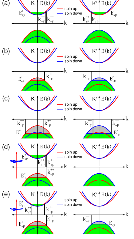
Figure 1: (Color online) Band structure in the $K$-valley (left column) and $K^{\prime}$-valley (right column) of the different ML-MoS₂ systems considered in this study. The bands are colored according to the spin type they represent. The green shading indicates electron occupation while the grey shading indicates hole occupation. In panels (a) - (c) only electrostatic gating is used to change the Fermi level of the systems. In panels (d) - (e) also right-handed circularly polarized light is added to the system in order to pump electrons in the $K$-valley from the valence to the conduction band. The Fermi vectors $k^{\varsigma s}_{\lambda\rm F}$ and Fermi energies $E_{\rm\lambda F}$ indicated follow Eqs. (II.1), (8)-(9) and (II.1)-(15).

II Theoretical approach

II.1 Electronic band structure and carrier concentration

In this study, we consider a ML-MoS₂ sheet positioned in the x-y plane. The effective Hamiltonian for a carrier (an electron or a hole) around the $K$ and $K^{\prime}$ points in reciprocal space can be written as Xiao12 ; Lu13

$$\hat{H}^{\varsigma}_{0}=\left(\begin{array}[]{cc}\Delta/2&\varsigma atk_{-\varsigma}\\ \varsigma atk_{\varsigma}&-\Delta/2+\varsigma s\gamma\\ \end{array}\right),$$ (1)

where $\mathbf{k}=(k_{x},k_{y})$ being the wavevector, $k_{\pm}=k_{x}\pm ik_{y}=ke^{\pm i\theta}$, and $\theta$ is the angle between $\mathbf{k}$ and the $k_{x}$-axis, $\varsigma$ is the valley index with $\varsigma=+$ for $K$ and $\varsigma=-$ for the $K^{\prime}$ valley, the spin index $s=\pm$ for spin-up and spin-down states, the lattice parameter $a=3.193$ Å, the hopping parameter $t=1.1$ eV Xiao12 , the spin-orbit parameter $\gamma=75$ meV Zhu11 , and $\Delta$ is the direct band gap equal to 1.66 eV between the conduction and valence bands Xiao12 ; Lu13 . Notice that DFT calculations Kormanyos15 have attributed a slightly larger mass to the holes than to electrons in ML-MoS₂. This has not been accounted for in the model described above but is not expected to have a significant impact on the results presented.

The corresponding Schrödinger equation for ML-MoS₂ at valley $K$ or $K^{\prime}$ can be solved analytically and the eigenvalues are given by

$$E^{\varsigma s}_{\lambda\mathbf{k}}=\varsigma s\gamma/2+\lambda\Lambda^{\varsigma s}(\mathbf{k}),$$ (2)

where $\Lambda^{\varsigma s}(\mathbf{k})=[a^{2}t^{2}\mathbf{k}^{2}+\Delta_{\varsigma s}^{2}]^{1/2}$, $\Delta_{\varsigma s}=(\Delta-\varsigma s\gamma)/2$, and $\lambda=\pm$ refers to conduction/valence band. The corresponding eigenfunction for a carrier in conduction or valence bands near the $K$($K^{\prime}$) point denoted by $|\mathbf{k},\lambda\varsigma s\rangle$ can be written as

$$|\mathbf{k},+\varsigma s\rangle=[\cos(\vartheta_{\mathbf{k}}^{\varsigma s}/2),\varsigma\sin(\vartheta_{\mathbf{k}}^{\varsigma s}/2)e^{i\varsigma\theta}]e^{i\mathbf{k}\cdot\mathbf{r}},$$

$$|\mathbf{k},-\varsigma s\rangle=[-\sin(\vartheta_{\mathbf{k}}^{\varsigma s}/2),\varsigma\cos(\vartheta_{\mathbf{k}}^{\varsigma s}/2)e^{i\varsigma\theta}]e^{i\mathbf{k}\cdot\mathbf{r}},$$ (3)

respectively, in a form of row vector with

$$\cos\vartheta^{\varsigma s}_{\mathbf{k}}=\frac{\Delta_{\varsigma s}}{\sqrt{a^{2}t^{2}k^{2}+\Delta^{2}_{\varsigma s}}},\sin\vartheta^{\varsigma s}_{\mathbf{k}}=\frac{atk}{\sqrt{a^{2}t^{2}k^{2}+\Delta^{2}_{\varsigma s}}}.$$

The electron (hole) density $n^{\varsigma}_{\lambda}$ ($\lambda=+$ for conduction band and $\lambda=-$ for valence band) of ML-MoS₂ at valley $\varsigma$ can be written as

$$n^{\varsigma}_{\lambda}=\frac{1}{(2\pi)^{2}}\sum_{s=\pm}\int d\mathbf{k}^{2}[\delta_{\lambda,-1}+\lambda f_{\lambda}(E^{\varsigma s}_{\lambda\mathbf{k}})],$$ (4)

where $f_{\lambda}(E^{\varsigma s}_{\lambda\mathbf{k}})=[e^{(E^{\varsigma s}_{\lambda\mathbf{k}}-\mu^{\varsigma}_{\lambda})/k_{B}T}+1]^{-1}$ is the Fermi-Dirac distribution function for electrons and $\mu^{\varsigma}_{\lambda}$ is the chemical potential (or Fermi energy $E^{\varsigma}_{\lambda\mathrm{F}}$ at zero temperature) for electrons in conduction band or holes in valence band at $\varsigma$ valley for a photo-excited quasi-equilibrium system in the present study. At $T$=0 K, Eq. (4) reduces to the familiar relation between the carrier density and the Fermi vector $k^{\varsigma s}_{\lambda\mathrm{F}}$ for a specific conduction/valence subband with spin index $s$ and valley index $\varsigma$,

$$n^{\varsigma}_{\lambda}=\sum_{s=\pm}[k^{\varsigma s}_{\lambda\mathrm{F}}]^{2}/(4\pi).$$ (5)

As depicted in Fig. 1, one can use the Fermi level to generate charge carrier liquids with different spins. If the Fermi level lies above the top point of the lowest valence subband for a $p$-type ML-MoS₂ as shown in Fig. 1 (b), the lowest subband is fully occupied by electrons and the holes are only distributed in the upper valence subband. The hole density in the upper valence subband is denoted by $n^{\varsigma}_{-}$. This regime holds when the Fermi level satisfies $E^{\varsigma}_{-\mathrm{F}}\geq-\Delta/2-\gamma$, which corresponds to a hole density $n^{\varsigma}_{-}\leq(\gamma^{2}+\Delta\gamma)/(2\pi a^{2}t^{2})=1.679\times 10^{13}$ cm^-2 at $\varsigma$ valley. The Fermi wave vector and Fermi level for the upper valence subband at valley $\varsigma$ are given by

$$[k^{\varsigma s}_{-\mathrm{F}}]^{2}=4\pi n^{\varsigma}_{-}(\varsigma s=1),$$

$$E^{\varsigma}_{-\mathrm{F}}=\gamma/2-[4\pi a^{2}t^{2}n^{\varsigma}_{-}+(\Delta-\gamma)^{2}/4]^{1/2}.$$ (6)

Then, we consider the other situations as shown in Fig. 1(a) and Fig. 1(c). Using the relation that the Fermi energies for Fermi wavevectors of spin-up and spin-down subbands should be equal, we obtain

$$\Lambda^{\varsigma-}(k^{\varsigma-}_{\lambda\mathrm{F}})-\Lambda^{\varsigma+}(k^{\varsigma+}_{\lambda\mathrm{F}})=\varsigma\lambda\gamma.$$ (7)

After combining Eqs. (5) and (7), one can derive the roots of $[k^{\varsigma s}_{\lambda\mathrm{F}}]^{2}$ as

$$[k^{\varsigma s}_{\lambda\mathrm{F}}]^{2}=2\pi n^{\varsigma}_{\lambda}+\varsigma s\bigg{[}\frac{\Delta\gamma}{2a^{2}t^{2}}-\lambda\frac{[\Delta^{2}\gamma^{2}+8\pi n^{\varsigma}_{\lambda}a^{2}t^{2}\gamma^{2}]^{1/2}}{2a^{2}t^{2}}\bigg{]}.$$ (8)

Thus, the Fermi energy for a zero temperature system at valley $\varsigma$ with a carrier density $n^{\varsigma}_{\lambda}$ is given by

$$E^{\varsigma}_{\lambda\mathrm{F}}=\varsigma s\gamma/2+\lambda\Lambda^{\varsigma s}(k^{\varsigma s}_{\lambda\mathrm{F}}).$$ (9)

The carrier density in a specific electronic branch can also be written as

$$n_{\lambda}^{\varsigma s}=\frac{n^{\varsigma}_{\lambda}}{2}+\varsigma s\bigg{[}\frac{\Delta\gamma}{8\pi a^{2}t^{2}}-\frac{\lambda[\Delta^{2}\gamma^{2}+8\pi n^{\varsigma}_{\lambda}\gamma^{2}a^{2}t^{2}]^{1/2}}{8\pi a^{2}t^{2}}\bigg{]}.$$ (10)

The density of state (DOS) can be presented by the imaginary part of the Green function as

$$D_{\lambda}(E)=\sum_{\varsigma s}\frac{|E|-\lambda\varsigma s\gamma/2}{2\pi a^{2}t^{2}}\theta[|E|-\lambda\varsigma s\gamma/2-\Delta_{\varsigma s}].$$ (11)

When the carrier concentration is low, one can expand Eq. (2) for small deviations from the $K$ or $K^{\prime}$ point. In that case, the low energy electronic band structure of ML-MoS₂ can be written as the 2DPB form for free electron/hole gases as

$$\tilde{E}^{\varsigma s}_{\lambda\mathbf{k}}=\lambda\frac{a^{2}t^{2}\mathbf{k}^{2}}{2\Delta_{\varsigma s}}+\lambda\Delta_{\varsigma s}+\frac{\varsigma s\gamma}{2},$$ (12)

and the DOS is given by

$$\tilde{D}_{\lambda}(E)=\sum_{\varsigma s}\frac{\Delta_{\varsigma s}}{2\pi a^{2}t^{2}}\theta[|E|-\lambda\varsigma s\gamma/2-\Delta_{\varsigma s}].$$ (13)

For a $p$-type sample at valley $\varsigma$ with a hole density $n_{-}^{\varsigma}\leq(\Delta-\gamma)\gamma/(2\pi a^{2}t^{2})$, the Fermi vector and Fermi level for the upper valence band is

$$[\tilde{k}^{\varsigma s}_{-\mathrm{F}}]^{2}=4\pi n_{\lambda}^{\varsigma}(\varsigma s=1),$$

$$\tilde{E}^{\varsigma}_{-\mathrm{F}}=-4\pi a^{2}t^{2}n_{\lambda}^{\varsigma}/(\Delta-\gamma)-\Delta/2+\gamma.$$ (14)

For the other cases with $n$- or $p$-type doping, the Fermi vector and Fermi level for a specific spin and valley subband can be written as

$$[\tilde{k}^{\varsigma s}_{\lambda\mathrm{F}}]^{2}=2\pi n_{\lambda}^{\varsigma}-\varsigma s\bigg{[}\frac{2\pi n_{\lambda}^{\varsigma}\gamma}{\Delta}-\frac{(\Delta^{2}-\gamma^{2})\gamma}{a^{2}t^{2}\Delta}\delta_{\lambda,-1}\bigg{]},$$

$$\tilde{E}^{\varsigma}_{\lambda\mathrm{F}}=\lambda\frac{a^{2}t^{2}[\tilde{k}^{\varsigma s}_{\lambda\mathrm{F}}]^{2}}{2\Delta_{\varsigma s}}+\lambda\Delta_{\varsigma s}+\frac{\varsigma s\gamma}{2}.$$ (15)

II.2 Quasi-equilibrium system by optical pumping

In this section, we solve the Boltzmann equation to obtain the response of charge carriers with different spin- and valley indexes to circularly polarized light. This enables us to find the quasi-equilibrium electron and hole densities in each valley that will be used in the next section to investigate the plasmonic response.

Within the Coulomb gauge, the vector potential of a light field with left ($\nu=-$)/right ($\nu=+$) handed polarization is given by Ibanez-Azpiroz12

$$A_{\nu}(t)=\frac{F_{0}}{\sqrt{2}\omega}\sin(\omega t)(\hat{\mathbf{x}}+\nu i\hat{\mathbf{y}}).$$ (16)

Within first-order perturbation theory, the steady-state electronic transition rate of inter-band transitions between valence and conduction band induced by direct carrier-photon interaction can be obtained by using the Fermi’s golden rule, which reads

$$W^{\varsigma s,\mp}_{\nu,\lambda\lambda^{\prime}}(\mathbf{k},\mathbf{k^{\prime}})= \frac{2\pi}{\hbar}\bigg{(}\frac{eatF_{0}}{\sqrt{2}\hbar\omega}\bigg{)}^{2}\delta_{\mathbf{k},\mathbf{k^{\prime}}}\delta(E^{\varsigma s}_{\lambda^{\prime}\mathbf{k^{\prime}}}-E^{\varsigma s}_{\lambda\mathbf{k}}\mp\hbar\omega)$$

$$\times[\cos^{4}(\vartheta_{\mathbf{k}}^{\varsigma s}/2)\delta_{\varsigma\nu,1}+\sin^{4}(\vartheta_{\mathbf{k}}^{\varsigma s}/2)\delta_{\varsigma\nu,-1}],$$ (17)

where $\lambda^{\prime}=-\lambda$, the Delta function $\delta_{\varsigma\nu,\pm 1}$ indicates the valley-dependent selection rule for optical transitions in ML-MoS₂ under a circularly polarized light field, and the $\mp$ sign in the Delta function refers to absorption ($-$) or emission ($+$) of a photon with energy $\hbar\omega$.

Due to the fast spin relaxation, compared to the photo-excited carrier life time Mak14 ; Song13 ; Korn11 , the photo-excited system in this study can be considered as a quasi-equilibrium system where the carrier distributions in conduction and valence bands can be approximately described by the Fermi-Dirac function with separate chemical potentials for electrons in conduction band and holes in valence band. For nondegenerate statistics, the Boltzmann equation (BE) for each valley and spin subsystem takes the form

$$\frac{\partial f^{\varsigma s}_{\lambda}(\mathbf{k})}{\partial t}=\sum_{\lambda^{\prime},\mathbf{k^{\prime}}}F_{\nu}^{\varsigma s}(\mathbf{k},\mathbf{k^{\prime}})-\frac{f^{\varsigma s}_{\lambda}(\mathbf{k})-f^{\varsigma s}_{\lambda 0}(\mathbf{k})}{\tau},$$ (18)

with $F_{\nu}^{\varsigma s}(\mathbf{k},\mathbf{k^{\prime}})=[W^{\varsigma s,-}_{\nu,\lambda^{\prime}\lambda}(\mathbf{k},\mathbf{k^{\prime}})+W^{\varsigma s,+}_{\nu,\lambda^{\prime}\lambda}(\mathbf{k},\mathbf{k^{\prime}})][f^{\varsigma s}_{\lambda^{\prime}}(\mathbf{k^{\prime}})-f^{\varsigma s}_{\lambda}(\mathbf{k})]$, and $f^{\varsigma s}_{\lambda}(\mathbf{k})\simeq f_{\lambda}(E_{\lambda\mathbf{k}}^{\varsigma s})$ is the carrier momentum distribution function and $f^{\varsigma s}_{\lambda 0}(\mathbf{k})$ represents the initial state in the presence of a dark system.

For the first moment, the mass-balance equation (or rate equation) can be derived after summing both sides of the BE over spin and wave vector. This leads to

$$\frac{\partial n^{\varsigma}_{+}}{\partial t}=\frac{\partial n^{\varsigma}_{-}}{\partial t}= \sum_{s}G_{\nu}^{\varsigma s}-\frac{\Delta n^{\varsigma}}{\tau},$$ (19)

where the carrier generation rate within each subsystem is

$$G^{\varsigma s}_{\nu}= \frac{e^{2}F_{0}^{2}}{32\hbar^{2}\omega}\bigg{[}1+\nu\varsigma\frac{2\Delta_{\varsigma s}}{\hbar\omega}\bigg{]}^{2}\theta(\hbar\omega-2\Delta_{\varsigma s})$$

$$\times\bigg{[}f_{-}\bigg{(}\frac{\varsigma s\gamma-\hbar\omega}{2}\bigg{)}-f_{+}\bigg{(}\frac{\varsigma s\gamma+\hbar\omega}{2}\bigg{)}\bigg{]},$$ (20)

$\Delta n^{\varsigma}$ is the photo-excited carrier density and $\tau$ is the photo-excited carrier life time which can be measured experimentally Korn11 . In the steady quasi-equilibrium state of the system, i.e., for $dn^{\varsigma}_{+}/dt=dn^{\varsigma}_{-}/dt=0$, the mass-balance equation at valley $\varsigma$ becomes

$$\Delta n^{\varsigma}=\tau\sum_{s}G_{\nu}^{\varsigma s}.$$ (21)

When one pumps the system with a circularly polarized optical beam, the electrons in the valence band are excited into the conduction band such that a gas of photo-excited carriers is formed in the conduction band. Therefore, the chemical potential for electrons/holes in conduction/valence band for each valley can be determined through

$$n^{\varsigma}_{\lambda} =n^{\varsigma}_{\lambda 0}+\Delta n^{\varsigma}.$$ (22)

where $n^{\varsigma}_{\lambda 0}$ is the initial carrier density in conduction or valence band. After combining Eqs. (21) and (22), the photo-excited carrier density can be determined.

From this, also the optical conductivity can be obtained as

$$\sigma^{\varsigma s}_{\nu}(\omega)= \frac{2\hbar\omega G^{\varsigma s}_{\nu}}{F_{0}^{2}}=\sigma_{0}\bigg{[}1+\varsigma\nu\frac{2\Delta_{\varsigma s}}{\hbar\omega}\bigg{]}^{2}\theta(\hbar\omega-2\Delta_{\varsigma s})$$

$$\times\bigg{[}f_{-}\bigg{(}\frac{\varsigma s\gamma-\hbar\omega}{2}\bigg{)}-f_{+}\bigg{(}\frac{\varsigma s\gamma+\hbar\omega}{2}\bigg{)}\bigg{]},$$ (23)

where $\sigma_{0}=e^{2}/(16\hbar)$. Finally, we can define the degree of valley-dependent absorption (VA) for light with polarization $\nu$ as

$$P_{\nu}(\omega)=\frac{\sum_{s}[\sigma^{+s}_{\nu}(\omega)-\sigma^{-s}_{\nu}(\omega)]}{\sum_{s}[\sigma^{+s}_{\nu}(\omega)+\sigma^{-s}_{\nu}(\omega)]}.$$ (24)

This quantity describes the difference between the absorption (or photo-excited carrier density) at $K$ and $K^{\prime}$ valleys under circularly polarized optical pumping.

II.3 Polarization function and plasmons

In this section, we set up the theoretical framework to calculate plasmons in a multi-component system. We work within the Random Phase Approximation (RPA).

When the degeneracy of spin or valley degrees of freedom of a electron/hole gas system is broken, it can be regarded as a multi-component system. For a multi-component system, the component-resolved response functions $\Pi^{i,i^{\prime}}(\mathbf{q},\omega)$ of the interacting electron liquid are given, in the RPA, by the following matrix equation Giuliani05 ; Agarwal14

$$[\Pi^{i,i^{\prime}}(\mathbf{q},\omega)]^{-1}=\{\Pi^{i}(\mathbf{q},\omega)\}^{-1}\delta_{i,i^{\prime}}-v_{q},$$ (25)

where $\Pi^{i}(\mathbf{q},\omega)$ is the non-interacting response function for the $i$-th component system and $v_{q}=e^{2}/(2\epsilon_{\mathrm{r}}\epsilon_{0}q)$ is the Fourier transform of the Coulomb interaction with $\epsilon_{\rm r}=5$ the relative dielectric constant of the background Scholz13 ; Kechedzhi14 . The total density-density response function within the RPA can then be written as

$$\Pi^{\mathrm{RPA}}(\mathbf{q},\omega)=\sum_{ii^{\prime}}\Pi^{i,i^{\prime}}(\mathbf{q},\omega)=\sum_{i}\Pi^{i}(\mathbf{q},\omega)/\epsilon_{\mathrm{RPA}}(\mathbf{q},\omega),$$ (26)

where the RPA dielectric function is defined as

$$\epsilon_{\mathrm{RPA}}(\mathbf{q},\omega)=1-v_{q}\sum_{i}\Pi^{i}(\mathbf{q},\omega).$$ (27)

Plasmons in the RPA can be found from the zeros of the dielectric function $\epsilon_{\mathrm{RPA}}(\mathbf{q},\omega(q)-i\eta)$, where $\omega(q)$ is the plasmon frequency and $\eta$ the decay rate of the plasmon Pyatkovskiy09 . Usually, plasmons can be approximately determined by the roots of the real part dielectric function $\mathrm{Re}[\epsilon_{\mathrm{RPA}}(\mathbf{q},\omega)]=0$ VanDuppen14 ; Tabert14 , which should also lead to resonance peaks in the energy loss function $\mathrm{Los}(\mathbf{q},\omega)=-\mathrm{Im}[\epsilon_{\mathrm{RPA}}]^{-1}$ that can be measured by means of electron energy loss spectroscopy (EELS) Politano14 . The decay rate (inverse life time) of the weakly damped plasmon is given by

$$\eta=\frac{\mathrm{Im}[\Pi(\mathbf{q},\omega(q))]}{\{(\partial/\partial\omega)\mathrm{Re}[\Pi(\mathbf{q},\omega)]\}_{\omega=\omega(q)}}.$$ (28)

The imaginary part of the dynamical RPA polarization near the undamped plasmon branch is given by Giuliani05 ; VanDuppen14

$$\mathrm{Im}[\Pi^{\mathrm{RPA}}(\mathbf{q},\omega(q))]=-O(\omega(q))\delta(\omega-\omega(q)),$$ (29)

and the oscillator strength of the undamped plasmon mode is defined as

$$O(\omega(q))=\frac{-\pi}{v_{q}}\frac{\mathrm{Re}[\Pi(\mathbf{q},\omega(q))]}{\{(\partial/\partial\omega)\mathrm{Re}[\Pi(\mathbf{q},\omega)]\}_{\omega=\omega(q)}}.$$ (30)

We use the strength of the absorption spectral function $A(\mathbf{q},\omega)=-\mathrm{Im}[\Pi^{\mathrm{RPA}}(\mathbf{q},\omega)]$ Kechedzhi14 to describe the oscillator strength of the damped plasmon modes in the particle-hole excitation spectrum (PHES) ($\mathrm{Im}[\Pi(\mathbf{q},\omega)]\neq 0$).

For both the undamped and weakly damped plasmon modes, the amplitude of the plasmon oscillation of each component $N(i)$ can be obtained by calculating the eigenmodes Agarwal14 of the real part of the matrix equation (25)

$$[\{\mathrm{Re}[\Pi^{i}(\mathbf{q},\omega(q))]\}^{-1}\delta_{i,i^{\prime}}-v_{q}]N(i)=0,$$ (31)

from which we can get the ratio of the plasmon oscillation amplitude

$$N(i)/N(i^{\prime})=\mathrm{Re}[\Pi^{i}(\mathbf{q},\omega(q))]/\mathrm{Re}[\Pi^{i^{\prime}}(\mathbf{q},\omega(q))].$$ (32)

We now turn to the calculation of the non-interacting response functions for each component $\Pi^{i}$. We denote each component by the spin and valley index, i.e. $i=\varsigma,s$ and find

$$\Pi^{\varsigma s}(\mathbf{q},\omega)=\sum_{\lambda\lambda^{\prime}\mathbf{k}}\frac{f(E^{\varsigma s}_{\lambda\mathbf{k}})-f(E^{\varsigma s}_{\lambda^{\prime}\mathbf{k+q}})}{\hbar\omega+E^{\varsigma s}_{\lambda\mathbf{k}}-E^{\varsigma s}_{\lambda^{\prime}\mathbf{k+q}}+i\delta}C^{\varsigma s}_{\lambda\mathbf{k},\lambda^{\prime}\mathbf{k+q}},$$ (33)

where the structure factor

$$C^{\varsigma s}_{\lambda\mathbf{k},\lambda^{\prime}\mathbf{k+q}}=\frac{1}{2}\bigg{[}1+\lambda\lambda^{\prime}\frac{\Delta_{\varsigma s}^{2}+a^{2}t^{2}\mathbf{k}(\mathbf{k+q})}{\Lambda^{\varsigma s}(\mathbf{k})\Lambda^{\varsigma s}(\mathbf{k+q})}\bigg{]},$$ (34)

with $\varphi$ the angle between $\mathbf{k}$ and $\mathbf{k+q}$ with $\cos\varphi=(k+q\cos\phi)/|\mathbf{k+q}|$, $\phi$ is the angle between $\mathbf{k}$ and $\mathbf{q}$, and $f(E^{\varsigma s}_{\lambda\mathbf{k}})=f_{\lambda}(E^{\varsigma s}_{\lambda\mathbf{k}})$ is the Fermi-Dirac distribution function for electrons.

At long-wavelength ($\mathbf{q}\rightarrow 0$) and low-temperature ($T\rightarrow 0$ K), we can expand Eq. (34) to second order in $q$:

$$C^{\varsigma s}_{\lambda\mathbf{k},\lambda^{\prime}\mathbf{k+q}}\simeq\delta_{\lambda,\lambda^{\prime}}-\lambda\lambda^{\prime}\sin^{2}(\vartheta_{\mathbf{k}}^{\varsigma s})q^{2}\sin^{2}\phi/(4k^{2}).$$ (35)

For intra-band transitions ($\lambda^{\prime}=\lambda$), the Lindhard ratio can be expanded to second order in $q$ with the result

$$\frac{f(E^{\varsigma s}_{\lambda\mathbf{k}})-f(E^{\varsigma s}_{\lambda\mathbf{k+q}})}{\hbar\omega+E^{\varsigma s}_{\lambda\mathbf{k}}-E^{\varsigma s}_{\lambda\mathbf{k+q}}}= q\cos\phi\delta(E^{\varsigma s}_{\lambda\mathbf{k}}-E^{\varsigma}_{\lambda\mathrm{F}})\frac{\partial E^{\varsigma s}_{\lambda\mathbf{k}}}{\partial k}$$

$$\times\bigg{(}\frac{1}{\hbar\omega}+\frac{q\cos\phi}{\hbar^{2}\omega^{2}}\frac{\partial E^{\varsigma s}_{\lambda\mathbf{k}}}{\partial k}\bigg{)}.$$ (36)

Because $C^{\varsigma s}_{\lambda\mathbf{k},\lambda^{\prime}\mathbf{k+q}}\simeq 1$ in the long-wavelength limit, we obtain the real part of the intra-band part of the polarization function as

$$\mathrm{Re}[\Pi_{\mathrm{intra}}(\mathbf{q},\omega)]= \frac{q^{2}}{4\pi\hbar^{2}\omega^{2}}\sum_{\lambda\varsigma s}(u^{\lambda}_{\varsigma s}-\Delta^{2}_{\varsigma s}/u^{\lambda}_{\varsigma s})$$

$$\times\theta(u^{\lambda}_{\varsigma s}-\Delta_{\varsigma s}),$$ (37)

with $u^{\lambda}_{\varsigma s}=|E^{\varsigma}_{\lambda\mathrm{F}}|-\lambda\varsigma s\gamma/2$ where $E^{\varsigma}_{\lambda\mathrm{F}}$ is the Fermi energy for electrons ($\lambda=1$) in the conduction band or holes ($\lambda=-1$) in the valence band.

For inter-band transitions ($\lambda^{\prime}=-\lambda$), the real part of the polarization function can be expanded to second order in $q$ with

$$\mathrm{Re}[\Pi_{\mathrm{inter}}(\mathbf{q},\omega)]= \frac{-q^{2}}{32\pi\hbar\omega}\sum_{\lambda\varsigma s}\ln\bigg{|}\frac{\hbar\omega+2u^{\lambda}_{\varsigma s}}{\hbar\omega-2u^{\lambda}_{\varsigma s}}\bigg{|}$$

$$\times\theta(u^{\lambda}_{\varsigma s}-\Delta_{\varsigma s}).$$ (38)

This only contributes by a small amount to the total polarization function in the low frequency regime where plasmons exist.

After using the low-$q$ expansion of the polarization function and neglecting the logarithmic correction, the charge plasmon dispersion in ML-MoS₂ is given by

$$\omega_{0}(q)=\big{[}e^{2}q\sum_{\lambda\varsigma s}(u^{\lambda}_{\varsigma s}-\Delta^{2}_{\varsigma s}/u^{\lambda}_{\varsigma s})\theta(u^{\lambda}_{\varsigma s}-\Delta_{\varsigma s})/(8\pi\epsilon_{\mathrm{r}}\epsilon_{0})\big{]}^{1/2}.$$ (39)

In order to calculate the polarization at arbitrary wave vector $q$, we note that the individual valley and spin resolved systems can be regarded as analogous to gapped graphene or silicene Pyatkovskiy09 ; VanDuppen14 ; Tabert14 . The polarization function depends on $u^{\lambda}_{\varsigma s}$ which corresponds to a shift of $\pm\gamma/2$ away from the absolute value of the Fermi level. At zero temperature, the polarization function of an electron liquid with spin $s$ in the $\varsigma$ valley can be written as

$$\Pi_{T=0}^{\varsigma s}(\mathbf{q},\omega)= \Pi^{\varsigma s}_{0,T=0}(\mathbf{q},\omega)[\tilde{\theta}(\Delta_{\varsigma s}-u^{-}_{\varsigma s})\tilde{\theta}(\Delta_{\varsigma s}-u^{+}_{\varsigma s})$$

$$-\theta(u^{-}_{\varsigma s}-\Delta_{\varsigma s})\theta(u^{+}_{\varsigma s}-\Delta_{\varsigma s})]$$

$$+\sum_{\lambda}\Pi^{\varsigma s\lambda}_{1,T=0}(\mathbf{q},\omega)\theta(u^{\lambda}_{\varsigma s}-\Delta_{\varsigma s}),$$ (40)

with the step functions

$$\tilde{\theta}(x)=\bigg{\{}\begin{array}[]{c}1,x\geqslant 0\\ 0,x<0\\ \end{array},\theta(x)=\bigg{\{}\begin{array}[]{c}1,x>0\\ 0,x\leqslant 0\\ \end{array}.$$ (41)

The detailed polarization function in the ($q$-$\omega$) plane is presented in the Appendix.

Finally, we note that in order to calculate the response of the system at finite temperature, one can use the following identity to express the Fermi-Dirac function Maldague78

$$\frac{4k_{B}T}{e^{(E-\mu)/k_{B}T}+1}=\int_{-\infty}^{\infty}\frac{d\mu^{\prime}\theta(\mu^{\prime}-E)}{\cosh^{2}[(\mu^{\prime}-\mu)/2k_{B}T]}.$$ (42)

Thus, the polarization function could be obtained as an integral transformation of its corresponding zero-temperature polarization function as Tomadin13

$$\Pi {}^{\varsigma s}_{T}(\mathbf{q},\omega;\mu^{\varsigma}_{+},\mu^{\varsigma}_{-})=\int_{\Delta/2}^{\infty}\frac{d\mu^{\prime}\Pi^{\varsigma s+}_{1,T=0}(\mathbf{q},\omega)|_{E^{\varsigma}_{+\mathrm{F}}=\mu^{\prime}}}{4k_{B}T\cosh^{2}[(\mu^{\prime}-\mu^{\varsigma}_{+})/2k_{B}T]}$$

$$+\int^{C}_{-\infty}\frac{d\mu^{\prime}\Pi^{\varsigma s-}_{1,T=0}(\mathbf{q},\omega)|_{E^{\varsigma}_{-\mathrm{F}}=\mu^{\prime}}}{4k_{B}T\cosh^{2}[(\mu^{\prime}-\mu^{\varsigma}_{-})/2k_{B}T]}+\Pi^{\varsigma s}_{0,T=0}(\mathbf{q},\omega)$$

$$\times[\mathcal{F}_{T}(C-\mu^{\varsigma}_{-})-\mathcal{F}_{T}(\Delta/2-\mu^{\varsigma}_{+})],$$ (43)

where $C=\varsigma s\gamma-\Delta/2$ and $\mathcal{F}_{T}(x)=(e^{x/k_{B}T}+1)^{-1}$, and $\mu^{\varsigma}_{\lambda}$ is the chemical potential for conduction and valence bands at valley $\varsigma$ which can be obtained through Eq. (4).

If the ML-MoS₂ system has low carrier density, one can also use a two dimensional parabolic band (2DPB) model to describe the electronic structure as explained in the previous section. The polarization function and plasmons of ML-MoS₂ with the 2DPB model are presented in the Appendix.

III Results and discussions

In this study, we consider both $n$- and $p$-doped ML-MoS₂, in the presence and absence of circularly polarized light. We can safely ignore the Rashba spin-orbit coupling because it requires a strong external perpendicular electric field XiaoYM16 . Therefore, the optical field only couples to the orbital part of the wave function and the spin is conserved during optical transitions. It should be noted that the determination of the photo-excited density in the presence of circularly polarized light in Sec. II.2 is only suitable for a relatively weak light fields. For high carrier density generated by optical pumping, we extracted the photo-excited carrier density from experimental data Mak14 . In the following sections, we present numerical calculations for both the plasmon dispersion, energy loss function, plasmon decay rate, plasmon oscillator strength, absorption spectral function and plasmon oscillation ratio to understand the physical characteristics of plasmons in ML-MoS₂.

III.1 Optical absorption of circularly polarized light

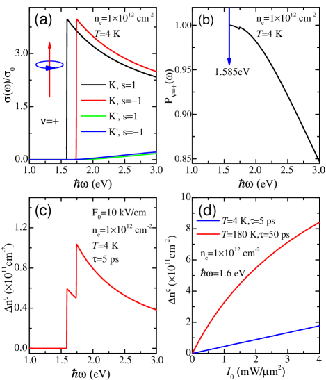
Figure 2: (Color online) (a) Contributions to the inter-band optical conductivity $\sigma^{\varsigma s}_{\nu}(\omega)$ for different valley and spin subsystems and (b) the VA of right-handed ($\nu=+1$) circularly polarized radiation by ML-MoS₂ as a function of photon energy. (c) Photo-excited carrier density due to right-handed circularly polarized light pumping at the $K$ valley as a function of photon energy. The sudden increase is due to the contribution from the spin-down subsystem. (d) Photo-excited carrier density at $K$ valley as a function of the radiation intensity $I_{0}\sim F^{2}_{0}$ of right-handed circularly polarized light with fixed photon energy, where $F_{0}$ is the electric field strength of the incident light.

In Fig. 2(a), we show the inter-band optical conductivity of an $n$-doped system generated by species of electrons with different valley and spin in response to a right-handed circularly polarized light beam ($\nu=+$). Correspondingly, the valley-dependent absorption (VA) is depicted in Fig. 2(b). The electron density is $n_{e}=1\times 10^{12}$ cm^-2, the system is assumed to be at low temperature, i.e. $T=4$ K and the lifetime of the photo-excited carriers is $\tau=$ 5 ps Korn11 . Fig. 2(a) shows that the optical conductivity, and hence the corresponding optical absorption, is the largest in the $K$ valley when the system is illuminated with right-handed polarized light. When the photon energy is near the edge of the band gap, absorption within the spin-up subband at the $K$ valley plays a dominant role while the absorption within the spin-down subband is suppressed. This is due to large spin splitting in the valence band. The VA in Fig. 2(b) decreases with increasing photon energy as more transitions become available. Notice the sudden increase in the VA curve which is due to the contribution from the inter-band transitions within the spin-down subband at the $K$ valley. We notice that one could obtain nearly 100$\%$ VA for a circularly polarized light with a photon frequency near the band gap Kioseoglou12 .

In Fig. 2(c), we show the photo-excited carrier density under right-handed circularly polarized light at the $K$ valley as a function of photon energy for a fixed strength of the electrical field. The photo-excited carrier density in Fig. 2(c) is proportional to the sum of the contributions to the spin and valley resolved optical conductivity presented in Fig. 2(a). In Fig. 2(d), we show the photo-excited carrier density in the $K$ valley as a function of the intensity of the incident radiation. In the presence of circularly polarized light with photon energy $\hbar\omega=$ 1.6 eV, the VA is nearly 100$\%$ which means only electrons in the $K$ valley are pumped. In the limit of weak light intensities, we observe that the photo-excited carrier density has a linear dependence on the radiation intensity, crossing over to a square root dependency for stronger radiation intensities when $T$=180 K. Notice that the photo-excited carrier life time varies with temperature Korn11 and that a larger carrier density can be obtained at higher temperature which can be seen from Eq. (21) and Fig. 2(d).

These results show that in order to efficiently excite charge carriers in a single valley, one has to use a circularly polarized light beam with photon energy close to the bandgap. This will break valley degeneracy in the ML-MoS₂ system and make it a multi-component system. The plasmonic response of these systems is discussed in the next sections.

III.2 Comparison between massive and hyperbolic description

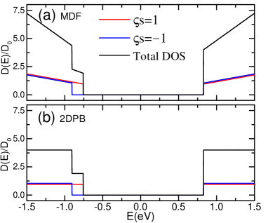
Figure 3: (Color online) Density of states for charge carriers in ML-MoS₂ with (a) MDF model and (b) 2DPB model, respectively. Here we used the notation $D_{0}=\Delta/(4\pi a^{2}t^{2})$.

Usually, the band structure of ML-MoS₂ is described by a massive Dirac Fermion (MDF) model Xiao12 . However, due to the large band gap in ML-MoS₂, the effective low-energy band structure of the MDF can also be approximately described by two-dimensional electron/hole gases with two-dimensional parabolic bands (2DPB) if the carrier concentration in the bands is not too large. The relation between these two models was shown before in Eq. (12). In this section we show the equivalence of these two models in describing the optical response of ML-MoS₂.

In Fig. 3, we plot the density of states (DOS) of ML-MoS₂ for MDF and 2DPB models, respectively. In the energy regime near the bottom/top of the conduction/valence band, the DOS of the two models is very close, while as the energy increases, the two models deviate from each other. This indicates that we can, indeed, use a 2DPB model to describe the band structure of ML-MoS₂ with low carrier density.

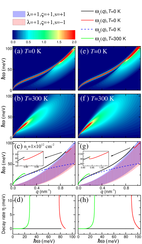
Figure 4: (Color online) The energy loss function for the MDF model at (a) $T=0$ K and (b) $T=300$ K. The plasmon dispersion and plasmon decay rate for the MDF model are shown in (c) and (d), respectively. (e)-(h) are the the corresponding results of (b)-(e) for the 2DPB model. The insets in (c) and (g) are a zoom of the large $q$ area as indicated by the arrows. The blue dashed curve corresponds to the zero temperature charge plasmon mode as obtained within the low-$q$ approximation.

In Fig. 4, we compare the plasmonic properties calculated within the two models for an $n$-type ML-MoS₂ whose band structure and occupation is shown in Fig. 1(a). We show the electron energy-loss function in the ($q$-$\omega$) plane at zero and room temperature, the plasmon dispersion and the decay rate of these modes. The electron density is fixed at $n_{e}=1\times 10^{12}$ cm^-2 and equally distributed over the two valleys. In Figs. 4(a) and (e), we compare the zero-temperature energy-loss functions. The plasmon appears as a curve of strong absorption in the long-wavelength limit. For large $q$, the plasmon branch merges with the continuum of intra-band single-carrier excitations, which shows up as an increased absorption. Notice that the two models give qualitatively the same results, and also quantitatively they agree very closely.

Panels (b) and (f) of Fig. 4 show the energy-loss function at room temperature. The result shows that a finite temperature damps the plasmon, inhibiting collective excitations at larger energies and wave vectors. Notice that also here the two models give qualitatively and quantitatively very similar results.

In panels (c) and (g) of Fig. 4 we show the roots of the real part of the dielectric function $\epsilon_{\rm PRA}(\mathbf{q},\omega)$ as solid curves. The black curve is the 2D charge plasmon, responsible for the thin line of enhanced absorption in the previous panels. As shown by the dashed blue curve, in the long-wavelength limit this mode coincides with the $\sqrt{q}$-plasmon mode from Eq. (39). The green solid curve in these panels shows the plasmon mode for a finite-temperature system. The results show that at room temperature this mode is limited to the long-wavelength regime. Remarkably, in both panels, shown by a solid red curve, there is also a new mode appearing inside the intra-band continuum of the spin-up/spin-down particles at $K$/$K^{\prime}$ valley. This new mode is responsible for the enhanced values of the electron-energy loss function in panels (a) and (e) and is not appearing only due to a breaking of the spin-degeneracy.

In panels (d) and (h) we show the decay rate as a function of the photon energy for each mode. The black solid curve at the bottom of the panel refers to the normal charge plasmon mode. The decay rate for this mode is zero for every energy because it lies outside the particle-hole continuum. The newly found mode, shown by the red curve, however, is partly Landau damped and acquires a finite decay rate. Notice that the decay rate decreases for larger energy and is of the same order of magnitude as that of the normal plasmon mode at room temperature, shown by the green curve in Figs. 4(d) and (h).

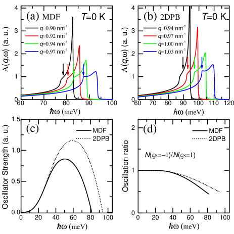
Figure 5: (Color online) The absorption spectral function of an $n$-type ML-MoS₂ for the situation corresponding to Fig. 4 as a function of energy for different fixed wavevectors for (a) the MDF model and (b) the 2DPB model at $T=0$ K. (c) The oscillator strength of the zero temperature undamped plasmon for the two models. (d) The oscillation ratio of the two different components in $n$-type ML-MoS₂ for the two models. The arrows in (a)-(b) indicate the corresponding plasmon frequency for the second plasmon branch $\omega_{2}(q)$.

In order to characterize the new, partly damped plasmon mode further, in Fig. 5, we show the spectral function $A(q,\omega)$ for different values of the wave vector $q$. We see that the new mode appears as a shoulder to the spectral function that should be distinguished from the peak in the spectral function at the edge of the particle-hole continuum. Panels (a) and (b) of Fig. 5 show that the MDF and 2DPB models have a qualitative correspondence, but quantitatively they differ slightly. This difference also surfaces when calculating the oscillator strength and the ratio of the amplitudes in both valleys in panels (c) and (d), respectively. It shows that the 2DPB model overestimates the oscillator strength and the plasmon frequency for a given wave vector. However, the qualitative behaviour is similar. We can, therefore, safely use the 2DPB model to investigate the plasmonic properties in ML-MoS₂ bearing in mind that the results might be quantitatively slightly departing.

III.3 Spin-polarized two-component system at finite temperature

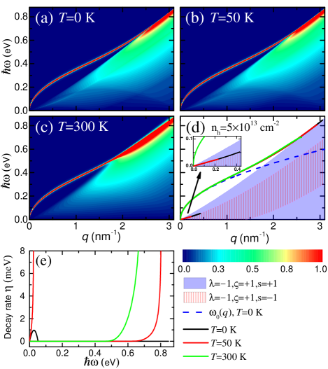
Figure 6: (Color online) (a)-(c) The energy loss function of strongly doped $p$-type ML-MoS₂ in the $(q,\omega)$ plane for different temperatures. (d) The plasmon dispersion as a function of wavevector for the different temperatures. (e) The plasmon decay rate as a function of plasmon energy for the plasmon modes in (c). The inset in (d) is the zoom of the small $q$ and $\omega$ regime as indicated by the arrow.

We now turn to the discussion of a two-component system where the two components are characterized by a different spin. We can obtain this system in MoS₂ by tuning the Fermi level such that the two spin resolved valence bands are occupied by holes as depicted in Fig. 1(c). Notice that because in the opposite valley the upper and lower valence bands are reversed, there is no macroscopic spin imbalance. Nonetheless, the spin-imbalance in a single valley has an effect on the optical and plasmonic properties of the system as will be shown below.

In Fig. 6 we show the energy loss function, plasmon dispersion and the plasmon decay rate for $p$-type ML-MoS₂ using the MDF model at a fixed hole density $n_{h}=5\times 10^{13}$ cm^-2. We show results for three different temperatures. The energy loss functions and corresponding plasmon dispersions at each temperature shows that there is a charge plasmon mode in the small $q$ regime. Notice, however, that in contrast to the $n$-type system, the plasmon dispersion is not affected a lot by temperature as is shown in Fig. 6(d). In panel (e), we show the decay rate of the plasmon modes at each temperature and find that also at finite temperature the lifetime is still appreciable, in strong contrast to $n$-type ML-MoS₂ discussed in the previous section.

The plasmon branches in Fig. 6(d) also reveal an additional peculiarity in the long-wavelength limit. Indeed, there exists a weakly damped linear acoustic plasmon mode in between the upper boundaries of the intra-band PHES of the two valence subbands. In this region the PHES has a local minimum and it is expected that the mode is, therefore, relatively stable. The distinct acoustic mode is similar to the one previously discussed in general spin-polarized two-dimensional electron gases Agarwal14 ; Kreil15 , but is now present in the absence of a macroscopic spin-imbalance and investigated at non-zero temperature.

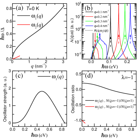
Figure 7: (Color online) (a) The plasmon dispersion as a function of wave vector for $p$-type ML-MoS₂ at $T=0$ K as shown in Fig. 6(d). (b) The absorption spectral function as a function of energy $\omega$ for fixed wavevectors and the absorption spectral function $A(q,\omega_{2}(q))$ (dashed line) for the linear acoustic plasmon $\omega_{2}(q)$. The solid and dashed arrows correspond to the weakly damped linear acoustic plasmon and undamped charge plasmon energies for fixed wavevectors. (c) Plasmon oscillator strength of the undamped plasmon mode $\omega_{1}(q)$. (d) Ratio of the plasmon oscillation amplitudes for the two spin components for the the two plasmon modes as indicated.

In Fig. 7(a), we show the plasmon dispersion of a $p$-type ML-MoS₂ for the MDF model with a fixed hole density $n_{h}=5\times 10^{13}$ cm^-2 as a function of wave vector for the zero temperature case as in Fig. 6(d). From this plot, one can clearly identify the normal $\omega_{1}(q)$ plasmon mode, and the acoustic mode $\omega_{2}(q)$. In Fig. 7(b), we plot the spectral function for fixed plasmon wave vectors. Notice that the linear plasmon mode appears as a peak on top of the background particle-hole weight and, therefore, is expected to be less clear than the distinct $\omega_{1}(q)$ plasmon. In panel (c) of Fig. 7, we show the oscillator strength of the $\omega_{1}(q)$ plasmon mode, which shows a similar behaviour as observed before.

To identify the character of the acoustic mode, in Fig. 7(d), we plot the ratio of the amplitude of the oscillation for both spin components. We see that for the new mode, displayed in red, this ratio is negative and approaches $-1$ in the long-wavelength limit. This means that the density of the two spin components oscillates in anti-phase. Therefore, this mode was labeled before as a spin-plasmon because this means that the carrier density does not oscillate, but it is rather the spin of the carriers that forms an oscillating pattern Agarwal14 . As a consequence of the carrier density oscillation being in anti-phase for each spin component, the mode is nearly charge neutral. Inspecting the $\omega_{1}(q)$ mode in panel (d) shows that the two spin-components oscillate in-phase for small frequency, but then cross-over to an oscillation in anti-phase. At this crossing point, the amplitude of the oscillation in the spin-down hole liquid is zero, and hence, the plasmon is spin-polarized.

III.4 Valley polarized three-component system

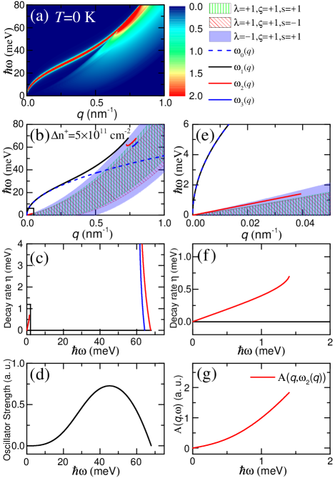
Figure 8: (Color online) (a) The energy loss function and (b) plasmons dispersion as a function of wave vector for an undoped ML-MoS₂ with a photo-excited carrier density $\Delta n^{+}=5\times 10^{11}$ cm^-2 by a right-handed circularly polarized optical pumping. (c) The corresponding plasmon decay rate as a function of plasmon energy. (e)-(f) are the zoom in of the black block areas in (c)-(d). (d) The plasmon oscillator strength of the undamped plasmon $\omega_{1}(q)$ as a function of plasmon energy. (g) The absorption spectral function of the weakly damped linear acoustic plasmon model $\omega_{2}(q)$.

In Fig. 8, we show the plasmonic behaviour of an undoped ML-MoS₂ sheet with a photo-excited carrier density $\Delta n^{+}=5\times 10^{11}$ cm^-2 by right-handed circularly polarized light at zero temperature. In Fig. 1(d), the band structure and carrier occupation are shown. In this system, free carriers exist only in the $K$ valley thanks to the valley-dependent photo-excitation. In the $K^{\prime}$ valley, no free carriers exist and, therefore, no plasmon propagation is possible.

This system can be regarded as a three-component system. Indeed, only one spin valence band is depleted by the photo-excitation, generating a single hole liquid, but because of very fast spin relaxation in the conduction band, both spin bands are occupied. This generates two independent free carrier liquids. For this system, the energy loss function in the ($q$-$\omega$) plane is shown in Fig. 8(a) and the plasmon dispersion as a function of $q$ is shown in Fig. 8(b). The plasmon branch shows up clearly in Fig. 8(a) and corresponds to an undamped charge plasmon mode. In Fig. 8(b), we can see that there exist now in total three plasmon modes in three regions divided by the upper boundaries of the intra-band PHES for the three components. These additional modes are responsible for the increased energy loss in that region in the $q-\omega$ plane. The corresponding plasmon decay rates are shown in Fig. 8(c) and show that the new plasmon modes have indeed a finite lifetime. The undamped charge plasmon mode $\omega_{1}(q)$, however has zero decay rate.

In the small $q$ limit, there is a weakly damped linear acoustic plasmon mode which we label by $\omega_{2}(q)$. To show this mode more clearly, in Figs. 8(e)-(f) we show a zoom of the black box in Figs. 8(b)-(c). Fig. 8(d) shows that the plasmon oscillator strength for $\omega_{1}(q)$ increases first and then decreases to zero. For the weakly damped linear acoustic plasmon mode $\omega_{2}(q)$ in the small $q$ regime, the plasmon decay rate and the strength of its absorption spectral function increase with increasing plasmon energy.

In Sec. II.3, we obtained the polarization function for each valley and spin subsystem of the MDF model which contains the contribution from both the intra-band transitions within the conduction and valence bands and the inter-band transitions between the conduction and valence bands. Thus, we cannot directly calculate the plasmon oscillation ratio of the different subband components through Eq. (32) with the polarization function of the MDF model for a photo-excited system. Instead, we resort to the description of the system with a 2DPB model.

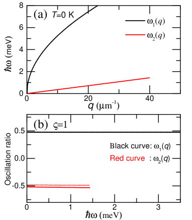
Figure 9: (Color online) (a) The plasmon dispersion within the 2DPB model of a photo-excited undoped ML-MoS₂. The carrier density $\Delta n^{+}=5\times 10^{11}$ cm^-2 is induced by right handed circularly polarized light pumping. (b) The oscillation ratio between the spin-up conduction subband at the $K$ valley and the spin-up valence subband at the $K$ valley (solid lines) and between the spin-down conduction subband at the $K$ valley and the spin-up valence subband at $K$ valley (dashed lines). The black and red curves correspond to the results of plasmon modes $\omega_{1}(q)$ and $\omega_{2}(q)$, respectively.

In Fig. 9, we show the plasmon dispersion and plasmon oscillation ratio for the corresponding situation shown in Fig. 8 but now with the 2DPB model. We find that the plasmon dispersion of 2DPB model in Fig. 9(a) coincides with the results in Fig. 8(e). Within the 2DPB model, we can calculate the ratio’s of the amplitude of oscillation in three different components considered in this system. In Fig. 9(b), we show these oscillation ratios as a function of the photon frequency. In these calculations, the amplitude of the oscillation is calculated with respect to the amplitude of the valence band component. For the undamped plasmon mode $\omega_{1}(q)$, the spin-up and spin-down components in the conduction band and the spin-up component in valence band at $K$ valley oscillate in phase. Both electron components have an equally large oscillation. For the linear plasmon mode $\omega_{2}(q)$, however, the oscillation ratio between the conduction band and valence band is negative so the oscillation is in anti-phase. In the low-$q$ limit, the summation of the oscillation ratio for the acoustic plasmon mode $\omega_{2}(q)$ with the spin-up and down conduction subbands is equal to $-1$. This means that the strength of the oscillation in both electron components is also nearly equal, but in anti-phase with the hole liquid. This type of anti-phase behavior was noted before in spin-polarized 2D electron systemsAgarwal14 . Now, however, the weakly damped linear plasmon is not charge neutral since the anti-phase oscillations occur in oppositely charged liquids of electrons and holes.

III.5 Four-component system

Figure 10: (Color online) (a) The energy loss function and (b) the plasmon dispersion as a function of wave vector for a photo-excited $p$-type doped ML-MoS₂ with initial hole density $n_{h}=1\times 10^{12}$ cm^-2 and a photo-excited carrier density $\Delta n^{+}=5\times 10^{11}$ cm^-2 induced by pumping with right-handed circularly polarized light. (c) The corresponding plasmon decay rate as a function of plasmon energy. (e) and (f) are the zoom of the black boxes in (b) and (c). (d) The plasmon oscillator strength of the undamped plasmon $\omega_{1}(q)$ as a function of plasmon energy. (g) The absorption spectral function of the two weakly damped linear acoustic plasmon modes.

We end the analysis with the discussion of a four-component system. As shown in Fig. 1(e), such a system can be created when a $p$-type ML-MoS₂ is pumped with circularly polarized light. This will excite electrons in one valley into the conduction band. As the spin relaxation time is very small Mak14 ; Song13 , the quasi equilibrium formed in the system consists of an electron pocket in one valley, but with electrons of two spin types with the same Fermi level, and two pockets of holes distributed over the two valleys with different Fermi level.

We assume that the $p$-type doped ML-MoS₂ has an initial hole density $n_{h}=1\times 10^{12}$ cm^-2. The photo-excited carrier density is $\Delta n^{+}=5\times 10^{11}$ cm^-2, which is induced by right-handed circularly polarized optical pumping. The energy loss function in Fig. 10(a) shows the typical plasmon pole corresponding to the $\omega_{1}(q)$ mode as in the previous systems. In Figs. 10(b) and (e) we, however, find that there exist three new plasmon branches for large photon energy, and two new acoustic modes in the long-wavelength limit. As before, these new modes appear in regions of the intra-band continuum where only some of the components are subject to Landau damping. The quantification of the importance of Landau damping is shown by the decay rate calculated in panels (c) and (f) where it is shown that, remarkably, the acoustic $\omega_{3}(q)$ mode is more stable than the acoustic $\omega_{2}(q)$ mode even though it can be found deeper in the intra-band electron-hole continuum. Furthermore, as shown in panel (g), the $\omega_{3}(q)$ mode is more pronounced in the spectral function than the $\omega_{2}(q)$, so one expects the former to be more easily excited. Finally, the oscillator strength calculated in panel (d) of Fig. 10 shows no qualitative differences due to the presence of the new modes in the intra-band continuum. This means that these modes are the consequence of a redistribution of spectral weight inside the continuum rather than getting it from the regular plasmon.

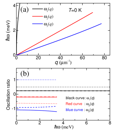
Figure 11: (Color online) (a) The zero-temperature plasmon dispersion within the 2DPB model of an optically pumped $p$-type doped ML-MoS₂ with a initial hole density $n_{h}=1\times 10^{12}$ cm^-2 and a photo-excited carrier density $\Delta n^{+}=5\times 10^{11}$ cm^-2 realized trough pumping with right-handed polarized light. (b) The ratio of the oscillation amplitudes in the spin-up conduction subband and the spin-up valence subband at $K$ valley (solid lines), the ratio between the spin-down conduction subband and the spin-up valence subband at $K$ valley (dashed lines) and the ratio between the spin-down valence subband at $K^{\prime}$ valley and the spin-up valence subband at $K$ valley (dotted lines). The black, red and blue curves correspond to the results of the plasmon modes $\omega_{1}(q)$, $\omega_{2}(q)$ and $\omega_{3}(q)$, respectively.

In Fig. 11, we plot the plasmon dispersion and the oscillation ratio between the different components for the long-wavelength acoustic modes discussed in the previous paragraph. For these results, we investigated the system within the 2DPB model. We find the same long-wavelength modes as before as we show in panel (a).

In panel (b), we calculate the ratio between the amplitudes of the different components in the system for the three different plasmon modes. The solid curves denote the ratio between the amplitude of the oscillations in the spin-up electron pocket and the spin-up hole pocket in the $K$ valley. The results show that the $\omega_{1}(q)$ mode consists of in-phase oscillations, while for the two other modes the oscillations are in anti-phase. The dashed curves in the same panel denote the ratio of the oscillation amplitude between the spin-down electron pocket and the hole pocket in the $K$-valley. For this, we find similar results as before, rendering the $\omega_{1}(q)$ mode in-phase, while the $\omega_{2}(q)$ and $\omega_{3}(q)$ modes are in anti-phase. Notice, however, that since we are now considering oscillations in the density of oppositely charged particles, it is the in-phased plasmon that compensate each others charged oscillation. Finally, the dotted curves show the ratio between the hole pockets in both valleys. Notice that, peculiarly, the $\omega_{3}(q)$ mode is completely in-phase and that the amplitude for both components is the same in this case. The $\omega_{1}(q)$ is also in-phase, as before, and the $\omega_{2}(q)$ mode is in anti-phase.

IV Conclusions

In this study, we examined the plasmonic response of a multi-component system. We took as a platform a ML-MoS₂ system subjected to circularly polarized light. We have shown that this system is capable of supporting multiple plasmon modes and we have quantified the effect of circular optical pumping within a Boltzmann framework.

We found that all platforms support a long-wavelength $\sqrt{q}$ plasmon branch at zero Kelvin. As temperature increases, we have shown that for an electron-doped system, the plasmon dispersion is strongly affected, while for a hole-doped system this mode is much more stable.

The main influence of having multiple components in the system is the appearance of distinct plasmonic modes that are partly damped. We found that for an $n$-component system, $n-1$ plasmon modes appear. These distinct modes manifest themselves in the long-wavelength limit as acoustic modes with a linear dispersion and are in a local minimum of the intra-band continuum. To evaluate their stability, we have calculated the decay rate for each of these modes and found that although they lie in the intra-band continuum, their lifetime is considerable. Furthermore, for larger wave vectors, we found that the multi-component system also supports new modes in regions where only some of the components are subject to Landau damping of the collective oscillation.

We evaluated the character of the modes by investigating the ratios of the amplitudes of the collective density oscillations of the different components. We found that the oscillation for the regular $\sqrt{q}$-mode is in-phase, while for the acoustic modes anti-phase oscillation is possible. Finally, we evaluated the spectral function, showing how the acoustic modes can be identified.

In the course of the investigation, we have shown that in the parameter range suitable for MoS₂ with optical pumping, the massive Dirac Fermion model and the 2D parabolic band model yield very similar results for the plasmonic response. This is because inter-band transitions do not to affect the plasmons very strongly.

Recently, experiments on the plasmonic response of MoS₂ have been performed using electron energy loss spectroscopy Wang2015 and angle-resolved reflectance spectroscopy Liu2016 . Also phonon-plasmon modes have been investigated using Fourier-transform infrared spectroscopy Patoka2016 . Applying these techniques to ML-MoS₂ with circularly polarized optical pumping one should be able to differentiate between the distinct plasmon modes and quantify their lifetime and oscillator strength.

The characteristic energy scale for plasmon modes in ML-MoS₂ covers not only the infrared but also the THz bandwidth, especially for the low frequency weakly damped linear acoustic plasmon modes. These properties make ML-MoS₂ a promising platform for plasmonic applications in the infrared and THz frequency regime. The theoretical investigations in this paper will help to guide the experimental search for new plasmon modes in ML-MoS₂ systems.

APPENDIX: ANALYTICAL EXPRESSION OF POLARIZATION FUNCTION

We use $\omega$ and $k$ as dimensionless variables to represent $\hbar\omega$ and $atk$ for notational simplification. For zero doping, the polarization function for spin $s$ band at $\varsigma$ valley is Pyatkovskiy09

$$\Pi^{\varsigma s}_{0,T=0}(\mathbf{q},\omega)= -\frac{q^{2}}{4\pi a^{2}t^{2}}\bigg{\{}\frac{\Delta_{\varsigma s}}{q^{2}-\omega^{2}}+\frac{q^{2}-\omega^{2}-4\Delta^{2}_{\varsigma s}}{4|q^{2}-\omega^{2}|^{3/2}}$$

$$\times\bigg{[}\theta(q-\omega)\arccos{\frac{\omega^{2}-q^{2}+4\Delta_{\varsigma s}^{2}}{q^{2}-\omega^{2}+4\Delta_{\varsigma s}^{2}}}$$

$$-\theta(\omega-q)\ln{\frac{(\sqrt{\omega^{2}-q^{2}}+2\Delta_{\varsigma s})^{2}}{|\omega^{2}-q^{2}-4\Delta^{2}_{\varsigma s}|}}\bigg{]}\bigg{\}}$$

$$-i\frac{q^{2}\tilde{x}^{2}_{\varsigma s}\theta(\omega^{2}-q^{2}-4\Delta^{2}_{\varsigma s})}{16a^{2}t^{2}|\omega^{2}-q^{2}|^{1/2}},$$ (44)

where $\tilde{x}^{2}_{\varsigma s}=2-x^{2}_{\varsigma s}$ and $x_{\varsigma s}=\sqrt{|1+4\Delta^{2}_{\varsigma s}/(q^{2}-\omega^{2})|}$.

For finite doping ($\lambda=+$ for $n$-type doping and $\lambda=-$ for $p$-type doping), the polarization function for the spin $s$ band at $\varsigma$ valley is

$$\Pi^{\varsigma s\lambda}_{1,T=0}(\mathbf{q},\omega)= -\frac{u^{\lambda}_{\varsigma s}}{2\pi a^{2}t^{2}}+\frac{q^{2}}{16\pi a^{2}t^{2}|q^{2}-\omega^{2}|^{1/2}}$$

$$\times\begin{cases}iG_{>}(y_{-})-iG_{>}(y_{+}),&\mathrm{1A}\\ G_{<}(y_{-})-iG_{>}(y_{+}),&\mathrm{2A}\\ G_{<}(y_{+})+G_{<}(y_{-}),&\mathrm{3A}\\ G_{<}(y_{-})-G_{<}(y_{+}),&\mathrm{4A}\\ G_{>}(y_{+})-G_{>}(y_{-}),&\mathrm{1B}\\ G_{>}(y_{+})+iG_{<}(y_{-}),&\mathrm{2B}\\ G_{>}(y_{+})-G_{>}(-y_{-})-i\pi\tilde{x}^{2}_{\varsigma s},&\mathrm{3B}\\ G_{>}(y_{+})+G_{>}(-y_{-})-i\pi\tilde{x}^{2}_{\varsigma s},&\mathrm{4B}\\ G_{0}(y_{+})-G_{0}(y_{-}).&\mathrm{5B}\end{cases}$$ (45)

where $y_{\pm}=(2u^{\lambda}_{\varsigma s}\pm\omega)/q$, and

$$G_{<}(x)=x(x_{\varsigma s}^{2}-x^{2})^{1/2}+(x_{\varsigma s}^{2}-2)\arccos{(x/x_{\varsigma s})},$$

$$G_{>}(x)=x(x^{2}-x_{\varsigma s}^{2})^{1/2}+(x_{\varsigma s}^{2}-2)\mathrm{arccosh}(x/x_{\varsigma s}),$$

$$G_{0}(x)=x(x^{2}+x^{2}_{\varsigma s})^{1/2}+(-x^{2}_{\varsigma s}-2)\mathrm{arcsinh}(x/x_{\varsigma s}).$$

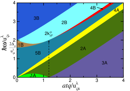
Figure 12: (Color online) The different regions with different expressions for the polarization function in Eq. (APPENDIX: ANALYTICAL EXPRESSION OF POLARIZATION FUNCTION). Here we have set $\Delta_{\varsigma s}=0.8u^{\lambda}_{\varsigma s}$.

The regions defining the polarization function in Eq. (APPENDIX: ANALYTICAL EXPRESSION OF POLARIZATION FUNCTION) are defined as

$$\mathrm{1A}: \omega\leq u^{\lambda}_{\varsigma s}-[(k^{\varsigma s}_{\lambda\mathrm{F}}-q)^{2}+\Delta_{\varsigma s}^{2}]^{1/2},$$

$$\mathrm{2A}: \mp u^{\lambda}_{\varsigma s}\pm[(k^{\varsigma s}_{\lambda\mathrm{F}}-q)^{2}+\Delta_{\varsigma s}^{2}]^{1/2}<\omega$$

$$\leq-u^{\lambda}_{\varsigma s}+[(k^{\varsigma s}_{\lambda\mathrm{F}}+q)^{2}+\Delta_{\varsigma s}^{2}]^{1/2},$$

$$\mathrm{3A}: \omega\leq-u^{\lambda}_{\varsigma s}+[(k^{\varsigma s}_{\lambda\mathrm{F}}-q)^{2}+\Delta_{\varsigma s}^{2}]^{1/2},$$

$$\mathrm{4A}: -u^{\lambda}_{\varsigma s}+[(k^{\varsigma s}_{\lambda\mathrm{F}}+q)^{2}+\Delta_{\varsigma s}^{2}]^{1/2}<\omega<q,$$

$$\mathrm{1B}: q\leq 2k^{\varsigma s}_{\lambda\mathrm{F}},[q^{2}+4\Delta_{\varsigma s}^{2}]^{1/2}<\omega$$

$$\leq u^{\lambda}_{\varsigma s}+[(k^{\varsigma s}_{\lambda\mathrm{F}}-q)^{2}+\Delta_{\varsigma s}^{2}]^{1/2},$$

$$\mathrm{2B}: u^{\lambda}_{\varsigma s}+[(k^{\varsigma s}_{\lambda\mathrm{F}}-q)^{2}+\Delta_{\varsigma s}^{2}]^{1/2}<\omega$$

$$\leq u^{\lambda}_{\varsigma s}+[(k^{\varsigma s}_{\lambda\mathrm{F}}+q)^{2}+\Delta_{\varsigma s}^{2}]^{1/2},$$

$$\mathrm{3B}: \omega>u^{\lambda}_{\varsigma s}+[(k^{\varsigma s}_{\lambda\mathrm{F}}+q)^{2}+\Delta_{\varsigma s}^{2}]^{1/2},$$

$$\mathrm{4B}: q>2k^{\varsigma s}_{\lambda\mathrm{F}},[q^{2}+4\Delta_{\varsigma s}^{2}]^{1/2}<\omega$$

$$\leq u^{\lambda}_{\varsigma s}+[(k^{\varsigma s}_{\lambda\mathrm{F}}-q)^{2}+\Delta_{\varsigma s}^{2}]^{1/2},$$

$$\mathrm{5B}: q<\omega\leq[q^{2}+4\Delta_{\varsigma s}^{2}]^{1/2}.$$

where the Fermi vector $k^{\varsigma s}_{\lambda\mathrm{F}}=\sqrt{|u^{\lambda}_{\varsigma s}|^{2}-\Delta_{\varsigma s}^{2}}$.

The polarization function for ML-MoS₂ calculated using the 2DPB model, Eq. (12), can be written as

$$\tilde{\Pi}(\mathbf{q},\omega)=\sum_{\varsigma s\lambda}\tilde{\Pi}_{\lambda}^{\varsigma s}(\mathbf{q},\omega),$$ (46)

where

$$\tilde{\Pi}_{\lambda}^{\varsigma s}(\mathbf{q},\omega)=\sum_{\mathbf{k}}\frac{f(\tilde{E}^{\varsigma s}_{\lambda\mathbf{k}})-f(\tilde{E}^{\varsigma s}_{\lambda\mathbf{k+q}})}{\omega+\tilde{E}^{\varsigma s}_{\lambda\mathbf{k}}-\tilde{E}^{\varsigma s}_{\lambda\mathbf{k+q}}+i\delta}.$$ (47)

At zero temperature, the real and imaginary part of the polarization function $\tilde{\Pi}_{\lambda,T=0}^{\varsigma s}(\mathbf{q},\omega)$ can be written separately as Stern67 ; Giuliani05

$$\mathrm{Re}\tilde{\Pi}^{\varsigma s}_{\lambda,T=0}(\mathbf{q},\omega)= -\frac{\Delta_{\varsigma s}}{2\pi a^{2}t^{2}}\bigg{[}1+\sum_{\alpha=\pm}\frac{\alpha\tilde{k}^{\varsigma s}_{\lambda\mathrm{F}}}{q}\theta(|\nu^{\varsigma s}_{\alpha}|^{2}-1)$$

$$\times\mathrm{sgn}[\nu^{\varsigma s}_{\alpha}]\sqrt{|\nu^{\varsigma s}_{\alpha}|^{2}-1}\bigg{]}\theta(\tilde{u}^{\lambda}_{\varsigma s}-\Delta_{\varsigma s}),$$

and

$$\mathrm{Im}\tilde{\Pi}^{\varsigma s}_{\lambda,T=0}(\mathbf{q},\omega)= -\frac{\Delta_{\varsigma s}}{2\pi a^{2}t^{2}}\sum_{\alpha=\pm}\frac{\alpha\tilde{k}^{\varsigma s}_{\lambda\mathrm{F}}}{q}\theta(1-|\nu^{\varsigma s}_{\alpha}|^{2})$$

$$\times\sqrt{1-|\nu^{\varsigma s}_{\alpha}|^{2}}\theta(\tilde{u}^{\lambda}_{\varsigma s}-\Delta_{\varsigma s}),$$ (48)

where $\tilde{u}^{\lambda}_{\varsigma s}=|\tilde{E}^{\varsigma}_{\lambda\mathrm{F}}|-\lambda\varsigma s\gamma/2$, the Fermi vector $\tilde{k}^{\varsigma s}_{\lambda\mathrm{F}}=\sqrt{2\Delta_{\varsigma s}(\tilde{u}^{\lambda}_{\varsigma s}-\Delta_{\varsigma s})}$, and

$$\nu^{\varsigma s}_{\alpha}=\frac{\omega\Delta_{\varsigma s}}{q\tilde{k}^{\varsigma s}_{\lambda\mathrm{F}}}-\alpha\frac{q}{2\tilde{k}^{\varsigma s}_{\lambda\mathrm{F}}}.$$ (49)

At zero temperature and in the low-$q$ approximation, the charge plasmon dispersion of ML-MoS₂ within the 2DPB model is

$$\tilde{\omega}_{0}(q)=\big{[}e^{2}q\sum_{\lambda\varsigma s}(\tilde{u}^{\lambda}_{\varsigma s}-\Delta_{\varsigma s})\theta(\tilde{u}^{\lambda}_{\varsigma s}-\Delta_{\varsigma s})/(4\pi\epsilon_{\mathrm{r}}\epsilon_{0})\big{]}^{1/2}.$$ (50)

At finite temperature, the full-$q$ polarization function is given by

$$\tilde{\Pi}^{\varsigma s}_{\lambda,T}(\mathbf{q},\omega;\tilde{\mu}^{\varsigma}_{\lambda})= \int_{-\infty}^{\infty}\frac{d\mu^{\prime}\tilde{\Pi}^{\varsigma s}_{\lambda,T=0}(\mathbf{q},\omega)|_{\tilde{E}^{\varsigma}_{\lambda\mathrm{F}}=\mu^{\prime}}}{4k_{B}T\cosh^{2}[(\tilde{\mu}^{\varsigma}_{\lambda}-\mu^{\prime})/2k_{B}T]}$$

$$\times\theta(|u^{\prime}|-\lambda\varsigma s\gamma/2-\Delta_{\varsigma s}),$$ (51)

where $\tilde{\mu}^{\varsigma}_{\lambda}$ is the chemical potential for conduction or valence subband which can be obtained through Eq. (4).

References

- (1) K. F. Mak, C. Lee, J. Hone, J. Shan, and T. F. Heinz, Phys. Rev. Lett. 105, 136805 (2010).
- (2) A. Splendiani, L. Sun, Y. Zhang, T. Li, J. Kim, C.-Y. Chim, G. Galli, and F. Wang, Nano Lett. 10, 1271 (2010).
- (3) Q. H. Wang, K. Kalantar-Zadeh, A. Kis, J. N. Coleman, and M. S. Strano, Nat. Nanotechnol. 7, 699 (2012).
- (4) B. Radisavljevic, M. B. Whitwick, and A. Kis, ACS Nano 5, 9934 (2011).
- (5) B. Radisavljevic, A. Radenovic, J. Brivio, V. Giacometti, and A. Kis, Nat. Nanotechnol. 6, 147 (2011).
- (6) S. B. Desai, S. R. Madhvapathy, A. B. Sachid, J. P. Llinas, Q. Wang, G. H. Ahn, G. Pitner, M. J. Kim, J. Bokor, C. Hu, H.-S. P. Wong, and A. Javey, Science 354, 99 (2016).
- (7) O. Lopez-Sanchez, D. Lembke, M. Kayci, A. Radenovic, and A. Kis, Nat. Nanotechnol. 8, 497 (2013).
- (8) H. S. Lee, S.-W. Min, Y.-G. Chang, M. K. Park, T. Nam, H. Kim, J. H. Kim, S. Ryu, and S. Im, Nano Lett. 12, 3695 (2012).
- (9) R. Ganatra and Q. Zhang, ACS Nano 8 (5), 4074 (2014).
- (10) H. Zeng, J. Dai, W. Yao, D. Xiao, and X. Cui, Nat. Nanotechnol. 7, 490 (2012).
- (11) K. F. Mak, K. He, J. Shan, and T. F. Heinz, Nat. Nanotechnol. 7, 494 (2012).
- (12) T. Cao, G. Wang, W. Han, H. Ye, C. Zhu, J. Shi, Q. Niu, P. Tan, E. Wang, B. Liu, and J. Feng, Nat. Commun. 3, 887 (2012).
- (13) K. F. Mak, K. L. McGill, J. Park, and P. L. McEuen, Science 344, 1489 (2014).
- (14) Z. Li and J. P. Carbotte, Phys. Rev. B 86, 205425 (2012).
- (15) P. M. Krstajić, P. Vasilopoulos, and M. Tahir, Phys. Rev. B 94, 085413 (2016).
- (16) Y. M. Xiao, W. Xu, B. Van Duppen, and F. M. Peeters, Phys. Rev. B 94, 155432 (2016).
- (17) K. He, N. Kumar, L. Zhao, Z. Wang, K. F. Mak, H. Zhao, and J. Shan, Phys. Rev. Lett. 113, 026803 (2014).
- (18) K. F. Mak, K. He, C. Lee, G. H. Lee, J. Hone, T. F. Heinz, and J. Shan, Nat. Mater. 12, 207 (2013).
- (19) H.-T. Chen, W. J. Padilla, J. M. O. Zide, A. C. Gossard, A. J. Taylor, and R. D. Averitt, Nature (London) 444, 597 (2006).
- (20) L. Ju, B. Geng, J. Horng, C. Girit, M. Martin, Z. Hao, H. A. Bechtel, X. Liang, A. Zettl, Y. R. Shen, and F. Wang, Nat. Nanotechnol. 6, 630 (2011).
- (21) K. S. Novoselov, A. K. Geim, S. V. Morozov, D. Jiang, Y. Zhang, S. V. Dubonos, I. V. Grigorieva, A. A. Firsov, Science 306, 666 (2004).
- (22) A. N. Grigorenko, M. Polini, and K. S. Novoselov, Nat. Photon. 6, 749 (2012).
- (23) F. H. L. Koppens, D. E. Chang, and F. J. Garcia de Abajo, Nano Lett. 11, 3370 (2011).
- (24) Z. Fei, A. S. Rodin, G. O. Andreev, W. Bao, A. S. McLeod, M. Wagner, L. M. Zhang, Z. Zhao, M. Thiemens, G. Dominguez, M. M. Fogler, A. H. Castro Neto, C. N. Lau, F. Keilmann, and D. N. Basov, Nature (London) 487, 82 (2012).
- (25) T. Low and P. Avouris, ACS Nano 8 (2), 1086 (2014).
- (26) B. Wunsch, T. Stauber, F. Sols, and F. Guinea, New J. Phys. 8, 318 (2006).
- (27) E. H. Hwang and S. Das Sarma, Phys. Rev. B 75, 205418 (2007).
- (28) P. K. Pyatkovskiy, J. Phys.: Condens. Matter 21, 025506 (2009).
- (29) A. Iurov, G. Gumbs, D. Huang, and V. M. Silkin, Phys. Rev. B 93, 035404 (2016).
- (30) B. Van Duppen, P. Vasilopoulos, and F. M. Peeters, Phys. Rev. B 90, 035142 (2014).
- (31) C. J. Tabert and E. J. Nicol, Phys. Rev. B 89, 195410 (2014).
- (32) A. Scholz, T. Stauber, and J. Schliemann, Phys. Rev. B 88, 035135 (2013).
- (33) K. Kechedzhi and D. S. L. Abergel, Phys. Rev. B 89, 235420 (2014).
- (34) H. Hatami, T. Kernreiter, and U. Zülicke, Phys. Rev. B 90, 045412 (2014).
- (35) F. Stern, Phys. Rev. Lett. 18, 546 (1967).
- (36) D. Xiao, G.-B. Liu, W. Feng, X. Xu, and W. Yao, Phys. Rev. Lett. 108, 196802 (2012).
- (37) H.-Z. Lu, W. Yao, D. Xiao, and S.-Q. Shen, Phys. Rev. Lett. 110, 016806 (2013).
- (38) A. Kormányos, V. Zólyomi, N. D. Drummond, and G. Burkard, Phys. Rev. X 4, 011034 (2014).
- (39) A. Kormányos, G. Burkard, M. Gmitra, J. Fabian, V. Zólyomi, N. D. Drummond, and V. Fal’ko, 2D Mater. 2, 022001 (2015).
- (40) G. F. Giuliani and G. Vignale, Quantum Theory of the Electron Liquid (Cambridge University Press, Cambridge, UK, 2005).
- (41) Z. Y. Zhu, Y. C. Cheng, and U. Schwingenschlögl, Phys. Rev. B 84, 153402 (2011).
- (42) J. Ibañez-Azpiroz, A. Eiguren, E. Ya. Sherman, and A. Bergara, Phys. Rev. Lett. 109, 156401 (2012).
- (43) Y. Song and H. Dery, Phys. Rev. Lett. 111, 026601 (2013).
- (44) T. Korn, S. Heydrich, M. Hirmer, J. Schmutzler, and C. Schüller, Appl. Phys. Lett. 99, 102109 (2011).
- (45) A. Agarwal, M. Polini, G. Vignale, and M. E. Flatté, Phys. Rev. B 90, 155409 (2014).
- (46) A. Politano and G. Chiarello, Nanoscale 6, 10927 (2014).
- (47) P. F. Maldague, Surface Science 73, 296 (1978).
- (48) A. Tomadin, D. Brida, G. Cerullo, A. C. Ferrari, and M. Polini, Phys. Rev. B 88, 035430 (2013).
- (49) G. Kioseoglou, A. T. Hanbicki, M. Currie, A. L. Friedman, D. Gunlycke, and B. T. Jonker, Appl. Phys. Lett. 101, 221907 (2012).
- (50) D. Kreil, R. Hobbiger, J. T. Drachta, and H. M. Böhm, Phys. Rev. B 92, 205426 (2015).
- (51) Y. Wang, J. Z. Ou, A. F. Chrimes, B. J. Carey, T. Daeneke, M. M. Y. A. Alsaif, M. Mortazavi, S. Zhuiykov, N. Medhekar, M. Bhaskaran, J. R. Friend, M. S. Strano, and K. Kalantar-Zadeh, Nano Lett. 15 883 (2015).
- (52) W. Liu, B. Lee, C. H. Naylor, H. Ee, J. Park, A. T. Charlie Johnson, and R. Agarwal, Nano Lett. 16, 1262 (2015).
- (53) P. Patoka, G. Ulrich, A. E. Nguyen, L. Bartels, P. A. Dowben, V. Turkowski, T. S. Rahman, P. Hermann, B. Kästner, A. Hoehl, G. Ulm, and E. Rühl, Opt. Express 24, 1154 (2016).