Landau-Zener transition in a two-level system coupled to a single highly-excited oscillator

Abstract

Two-level system strongly coupled to a single resonator mode (harmonic oscillator) is a paradigmatic model in many subfields of physics. We study theoretically the Landau-Zener transition in this model. Analytical solution for the transition probability is possible when the oscillator is highly excited, i.e. at high temperatures. Then the relative change of the excitation level of the oscillator in the course of the transition is small. The physical picture of the transition in the presence of coupling to the oscillator becomes transparent in the limiting cases of slow and fast oscillator. Slow oscillator effectively renormalizes the drive velocity. As a result, the transition probability either increases or decreases depending on the oscillator phase. The net effect is, however, the suppression of the transition probability. On the contrary, fast oscillator renormalizes the matrix element of the transition rather than the drive velocity. This renormalization makes the transition probability a non-monotonic function of the coupling amplitude.

I Introduction

Since the publication of seminal papers Caldeira ; Chakravarty , see also the review Ref. Review, , the effect of environment on the dynamics of a two-level system is modeled by introducing the coupling of the levels to the infinite set of harmonic oscillators.

In the course of the Landau-Zener (LZ) transition,Landau1932 ; Zener1932 ; Majorana ; Stueckelberg when the energy levels of the two-level system undergo the avoided crossing under the action of external drive, the effect of environment amounts to the loss of adiabaticity of the transition. More quantitatively, the probability for the system to stay in the ground state after the transition is diminished by the environment.Gefen ; Ao1991 ; Shimshoni ; Nalbach2009+ ; Pekola2011+ ; Ziman2011+ ; Vavilov2014+ ; Nalbach2014+ ; Nalbach2015+ ; Ogawa2017+ ; Arceci2017 ; we The underlying reason for this is the absorption of “quanta” of the environment. This absorption leads to decoherence, which suppresses the interference of different virtual tunneling pathways.

The situation is more delicate when the environment is represented by a single oscillator.Wubs2005++ ; Wubs2006++ ; WubsEPL ; Wubs2007++ ; Zueco ; Ashhab1 ; Ashhab2 ; Sinitsyn ; Sun In experiment, the role of such an oscillator, which is coupled to the two-level system, is played e.g. by the transmission line resonatorExperiment1 or by the optical resonator.Experiment2

In the absence of coupling, the amplitude of the LZ transition can be viewed as coherent superposition of many amplitudes corresponding to virtual trajectories. With coupling, each virtual transition is accompanied by the excitation of the oscillator. On the other hand, the stronger oscillator is excited, the stronger is the feedback that it exercises on the two-level system. Then it is a compound object, two-level system dressed by many oscillator quanta, that undergoes the LZ transition.

For the two-level system coupled to the environment with a continuous spectrum only the weak-coupling regime is of interest. This is because, upon increasing coupling, the interference is completely suppressed, so that the transition probability, $P_{\scriptscriptstyle LZ}$, assumes the value $P_{\scriptscriptstyle LZ}=1/2$. On the contrary, when the two level system is coupled to a single oscillator, there is a wide domain of parameters when the coupling is strong while $P_{\scriptscriptstyle LZ}$ is still a strong function of the drive velocity.

Nontriviality of the Landau-Zener (LZ) transition in the presence of coupling to the oscillator is highlighted by the exact result reported in Ref. Wubs2006++, . This result pertains strictly to zero temperature when at time $t\rightarrow-\infty$ the oscillators is in the ground state. It was demonstrated in Ref. Wubs2006++, that if the two-level system starts in the state $\uparrow$ and ends in the state $\uparrow$, then the oscillator remains in the ground state at $t\rightarrow\infty$. This result can be viewed as a manifestation of the “no-go” theoremSinitsyn2004 ; Shytov2004 ; Vitanov2005 in application to the spin-boson model. Certainly, at intermediate times, the oscillator can be excited. As a consequence of the above restriction, the two-level system and the oscillator end up entangled.

Another manifestation of nontriviality of the LZ transition with coupling to a single oscillator is the dependence of $P_{\scriptscriptstyle LZ}$ on the coupling strength, $g$. In particular, numerical results of Ref. Ashhab1, suggest that, for finite-temperature oscillator, the dependence of $P_{\scriptscriptstyle LZ}$ on $g$ is a non-monotonic curve with a minimum. In other words, upon increasing $g$, the adiabaticity of the transition first decreases and then increases again. There is no clear physical picture explaining the emergence of this minimum. In theory, coupling to the oscillator turns a single avoided crossing, taking place in the course of the LZ transition, into a network of avoided crossingsGaraninNetwork corresponding to different oscillator levels. The coupling strength quantifies the “talking” between the $\uparrow$ and $\downarrow$ amplitudes pertaining to a certain oscillator level to the corresponding amplitudes for two neighboring oscillator levels.

In general, the problem of the LZ transition in the presence of coupling to the oscillator contains, in addition to $g$, three other parameters with the dimensionality of frequency: the matrix element between $\uparrow$ and $\downarrow$ levels, the inverse bare LZ transition time, and the oscillator frequency. Definitely, it is impossible to derive an analytical expression for $P_{\scriptscriptstyle LZ}$ for arbitrary relations between these parameters. In the present paper we focus on the situation when the oscillator is highly excited. Under this simplifying assumption we identify the domain of parameters where the asymptotic analytical expression for $P_{\scriptscriptstyle LZ}$ can be found. Roughly speaking, the two domains correspond to slow and fast oscillator depending on whether the LZ transition time is shorter or longer than the oscillator period. Coupling to a slow oscillator effectively renormalizes the drive velocity. In the case of a fast oscillator, the LZ transition splits, as a results of coupling, into a sequence of individual transitions even-spaced in time. The corresponding gaps are the oscillating functions of coupling strength, $g$. Non-monotonic behavior of the survival probability with $g$ is the result of interference of partial transition amplitudes. We confirm this behavior by solving the many-level Schrödinger equation numerically.

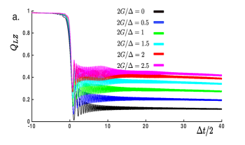
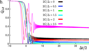
Figure 1: (Color online) Survival probability, $Q_{\scriptscriptstyle LZ}$, calculated numerically from the system Eq. (8) is plotted versus dimensionless time, $\Delta t/2$, for several values of the coupling amplitude, $G$, and for the oscillator phases $\kappa=\pi/2$ (a) and $\kappa=-\pi/2$ (b). The oscillator frequency is chosen to be $\omega=0.25\Delta$, where $\Delta$ is the gap at $t=0$, while the drive velocity is chosen to be $v=\pi\Delta^{2}/4$. At zero coupling, the survival probability at $t\rightarrow\infty$ is $Q_{\scriptscriptstyle LZ}(\infty)=e^{-2}$. For $\kappa=\pi/2$ the values $Q_{\scriptscriptstyle LZ}(\infty)$ grows monotonically with $G$, while for $\kappa=-\pi/2$ the value $Q_{\scriptscriptstyle LZ}(\infty)$ first drops with $G$ and then grows with $G$.

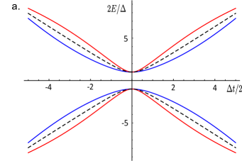
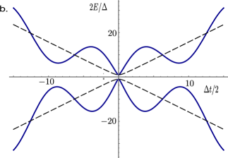
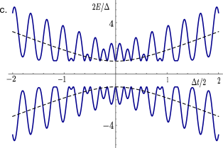
Figure 2: (Color online) The time-dependent energy levels Eq. (10) are plotted for $\kappa=\pi/2$ and different oscillator frequencies and the coupling strengths: (a) $G=0.25\Delta$, $\omega=0.25\Delta$; (b) $G=4\Delta$, $\omega=0.25\Delta$; (c) $G=0.5\Delta$, $\omega=10\Delta$. The level positions in the absence of coupling are shown with dashed lines. Three distinct shapes of the curves $E(t)$ illustrate three different scenarios of how the coupling to the oscillator affects the LZ transition. (a) and (b) correspond to the slow oscillator regime. In (a), the coupling amounts to effective modification of the drive velocity. Upon increasing the coupling, (b), the LZ transition is the result of interference of many isolated LZ transitions. For the fast oscillator, (c), the description of the LZ transition in terms of time-dependent energy levels is inadequate. Blue lines in (a) show the energy levels calculated for the same coupling and frequency as red lines but for $\kappa=-\pi/2$.

II Basic relations

We start from the standard Hamiltonian of the spin-boson model with drive

$${\hat{H}}=-\frac{vt}{2}{\hat{\sigma}_{z}}-\frac{\Delta}{2}{\hat{\sigma}_{x}}+\omega{\hat{b}}^{\dagger}{\hat{b}}+g{\hat{\sigma}_{z}}\otimes({\hat{b}}+{\hat{b}}^{\dagger}),$$ (1)

where $\omega$ is the oscillator frequency, while ${\hat{b}}$ and ${\hat{b}}^{\dagger}$ are, respectively, the annihilation and the creation operators of the oscillator. The drive is characterized by the rate, $v$, of the change of the energies of the $\uparrow$ and $\downarrow$ states coupled directly by the matrix element $\Delta/2$. It is assumed that the coupling between the two-level system and the oscillator is longitudinal.

Denote with $a_{\scriptscriptstyle 1}^{n}$ and $a_{\scriptscriptstyle 2}^{n}$ the amplitudes to find the system in the states $\uparrow$ and $\downarrow$ with $n$ quanta excited. As follows from Eq. (1), these amplitudes satisfy the following infinite system of coupled equations

$$i{\dot{a}}_{\scriptscriptstyle 1}^{n}+\frac{vt}{2}a_{\scriptscriptstyle 1}^{n}+\Big{(}n+\frac{1}{2}\Big{)}\omega a_{\scriptscriptstyle 1}^{n}-\frac{\Delta}{2}a_{\scriptscriptstyle 2}^{n}\\ =-g\Big{[}(n+1)^{\scriptscriptstyle 1/2}a_{\scriptscriptstyle 1}^{n+1}+n^{\scriptscriptstyle 1/2}a_{\scriptscriptstyle 1}^{n-1}\Big{]},$$ (2)

$$i{\dot{a}}_{\scriptscriptstyle 2}^{n}-\frac{vt}{2}a_{\scriptscriptstyle 2}^{n}+\Big{(}n+\frac{1}{2}\Big{)}\omega a_{\scriptscriptstyle 2}^{n}-\frac{\Delta}{2}a_{\scriptscriptstyle 1}^{n}\\ =g\Big{[}(n+1)^{\scriptscriptstyle 1/2}a_{\scriptscriptstyle 2}^{n+1}+n^{\scriptscriptstyle 1/2}a_{\scriptscriptstyle 2}^{n-1}\Big{]}.$$ (3)

Our goal is to find the analytical solution of this system in the limit when the oscillator is highly excited, so that the relevant $n$-values are big. In this limit, we can neglect the difference between $(n+1)^{\scriptscriptstyle 1/2}$ and $n^{\scriptscriptstyle 1/2}$. Denote the initial state of the oscillator with $n=n_{0}\gg 1$. A crucial simplification is achieved if, in the course of the transition, the excitation level of the oscillator changes relatively weakly, i.e. by $m$ quanta with $m$ much smaller than $n_{0}$. This allows to eliminate the explicit $n$-dependence from the system Eq. (3). Upon introducing the new variables

$$a_{\scriptscriptstyle 1}^{n}(t)=b_{\scriptscriptstyle 1}^{m}(t)\exp\Big{[}i\omega t\Big{(}n_{0}+m+\frac{1}{2}\Big{)}\Big{]},$$

$$a_{\scriptscriptstyle 2}^{n}(t)=b_{\scriptscriptstyle 2}^{m}(t)\exp\Big{[}i\omega t\Big{(}n_{0}+m+\frac{1}{2}\Big{)}\Big{]},$$ (4)

we get

$$i{\dot{b}}_{\scriptscriptstyle 1}^{m}+\frac{vt}{2}b_{\scriptscriptstyle 1}^{m}-\frac{\Delta}{2}b_{\scriptscriptstyle 2}^{m} = -G\Big{[}b_{\scriptscriptstyle 1}^{m+1}e^{i\omega t}+b_{\scriptscriptstyle 1}^{m-1}e^{-i\omega t}\Big{]},$$

$$i{\dot{b}}_{\scriptscriptstyle 2}^{m}-\frac{vt}{2}b_{\scriptscriptstyle 2}^{m}-\frac{\Delta}{2}b_{\scriptscriptstyle 1}^{m} = G\Big{[}b_{\scriptscriptstyle 1}^{m+1}e^{i\omega t}+b_{\scriptscriptstyle 1}^{m-1}e^{-i\omega t}\Big{]}.$$ (5)

where

$$G=gn_{0}^{\scriptscriptstyle 1/2}.$$ (6)

Obviously, the partial solutions of the system Eq. (5) are the plane waves

$$b_{\scriptscriptstyle 1}^{m}(t)=B_{\scriptscriptstyle 1}(t)e^{-i\kappa m},~{}~{}~{}b_{\scriptscriptstyle 2}^{m}(t)=B_{\scriptscriptstyle 2}(t)e^{-i\kappa m},$$ (7)

where $\kappa$ is the wave vector. The amplitudes $B_{\scriptscriptstyle 1}$, $B_{\scriptscriptstyle 2}$ satisfy the system

$$i{\dot{B}}_{\scriptscriptstyle 1}+\Big{[}\frac{vt}{2}+2G\cos(\omega t-\kappa)\Big{]}B_{\scriptscriptstyle 1}-\frac{\Delta}{2}B_{\scriptscriptstyle 2}=0,$$

$$i{\dot{B}}_{\scriptscriptstyle 2}-\Big{[}\frac{vt}{2}+2G\cos(\omega t-\kappa)\Big{]}B_{\scriptscriptstyle 2}-\frac{\Delta}{2}B_{\scriptscriptstyle 1}=0.$$ (8)

This system describes the LZ transition within a given $\kappa$. The form Eq. (8) suggests the interpretation of $\kappa$ as a phase of the classical oscillator.

Original system Eq. (3) describes the “spreading” of the initial state with $n=n_{0}$ over the states with $n=n_{0}+m$. The survival probability $Q_{\scriptscriptstyle LZ}^{n\rightarrow(n+m)}$ is the probability for the system, which starts at $t\rightarrow-\infty$ from a single nonzero amplitude $a_{\scriptscriptstyle 1}^{n_{0}}$, to remain in one of the states $a_{\scriptscriptstyle 1}^{n_{0}+m}$ at $t\rightarrow\infty$. After reducing the original system to the form Eq. (8) the amplitude $B_{\scriptscriptstyle 1}$ represents a combination $\sum\limits_{m}b_{\scriptscriptstyle 1}^{m}\exp(-i\kappa m)$. The initial condition that at $t\rightarrow-\infty$ the $m$-dependence of amplitude $b_{\scriptscriptstyle 1}^{m}$ is $\delta_{m,0}$ suggests that the solutions of Eq. (8) corresponding to different $\kappa$ have the same absolute value at $t\rightarrow-\infty$. This allows to express the net LZ survival probability via the survival probabilities corresponding to all $\kappa$-values

$$Q_{\scriptscriptstyle LZ}=1-P_{\scriptscriptstyle LZ}=\sum\limits_{m}Q_{\scriptscriptstyle LZ}^{n\rightarrow(n+m)}=\int\limits_{-\pi}^{\pi}\frac{d\kappa}{2\pi}Q_{\scriptscriptstyle LZ}(\kappa).$$ (9)

In the remainder of the paper we study the dependence of $Q_{\scriptscriptstyle LZ}$ found from Eqs. (8), (9) in the limits of slow and fast oscillator.

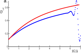
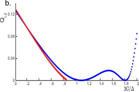
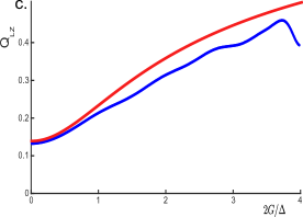
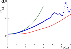
Figure 3: (Color online) The survival probability, $Q_{\scriptscriptstyle LZ}$, at $t\rightarrow\infty$ is plotted versus the dimensionless coupling strength for the phases of oscillator $\kappa=\pi/2$ (a), $\kappa=-\pi/2$ (b), and $\kappa=0$ (c). Blue curves were obtained by solving the system Eq. (8) numerically. Red curves are theoretical obtained from Eqs. (14), (15). In the lower panel (d) the result of the numerical averaging of $Q_{\scriptscriptstyle LZ}(\kappa)$ is plotted with blue line. The green line shows the analytical result Eq. (16), while the analytical result obtained from Eqs. (14), (15) is shown with red line. The drive velocity and the oscillator frequency are the same as in Fig. 1.

III Slow oscillator

To illustrate how delicate is the effect of coupling to the low-frequency oscillator on the survival probability, we plot in Figs. 1a, b the numerical solutions of the system Eq. (8) for different $G$-values. Fig. 1a corresponds to the wave vector $\kappa=\pi/2$, while Fig. 1b corresponds to $\kappa=-\pi/2$. The solutions $Q_{\scriptscriptstyle LZ}(t)$ correspond to the “subgap” frequency $\omega=0.25\Delta$. The drive velocity is chosen to be $v=\pi\Delta^{2}/4$, so that, without coupling, the survival probability $Q_{\scriptscriptstyle LZ}=\exp\left(-\pi\Delta^{2}/2v\right)$ is small, $Q_{\scriptscriptstyle LZ}=e^{-2}$. Comparing Figs. 1a and 1 b, we conclude that the effect of coupling on $Q_{\scriptscriptstyle LZ}$ is very different for these two values of $\kappa$. For $\kappa=\pi/2$ the survival probability increases monotonically with the coupling strength, $G$, while for $\kappa=-\pi/2$, already for the minimal coupling $G=0.25\Delta$, the value of $Q_{\scriptscriptstyle LZ}$ is smaller than in the absence of coupling.

Formal explanation of this peculiar dependence of $Q_{\scriptscriptstyle LZ}$ on $\kappa$ follows from the expression of the time-dependent energy levels of the system Eq. (8). This expression reads

$$E=\pm\Bigg{[}\frac{\Delta^{2}}{4}+\left(\frac{vt}{2}+2G\cos\left(\omega t-\kappa\right)\right)^{2}\Bigg{]}^{1/2}.$$ (10)

In Fig. 2a we plot these levels for $G=0.25\Delta$ and $\kappa=\pm\pi/2$. It is seen that the plots $E(t)$ for $\kappa=\pm\pi/2$ lie on the opposite sides of the $G=0$ curve. Thus, for $\kappa=\pi/2$, the coupling to the oscillator effectively increases the drive velocity, and, thus, $Q_{\scriptscriptstyle LZ}$ gets enhanced. For $\kappa=-\pi/2$, the effective drive velocity is decreased due to the coupling to the oscillator and, correspondingly, $Q_{\scriptscriptstyle LZ}$ is diminished,

Dramatic difference of the survival probabilities for different $\kappa$-values becomes even more dramatic upon further increase of coupling strength. This is illustrated in Fig. 3, where the curves $Q_{\scriptscriptstyle LZ}(G)$ obtained numerically are plotted for $\kappa=\pi/2$, $\kappa=-\pi/2$, and $\kappa=0$. While all three curves start from $Q_{\scriptscriptstyle LZ}=e^{-2}$, the $\kappa=\pi/2$ and $\kappa=0$ curves increase with $G$, while the $\kappa=-\pi/2$ curve decreases with $G$. It also follows from Fig. 3 that beyond certain $G$-value all three curves exhibit strong oscillations.

The goal of the theory is to account for the shapes of the curves. To this end, we recall that, in the absence of coupling, the most concise way to derive expression $Q_{\scriptscriptstyle LZ}=\exp\left(-\pi\Delta^{2}/2v\right)$ is to perform the analytic continuation of the semiclassical solutions, $\exp\left(\pm i\int\limits_{0}^{t}dt^{\prime}E(t^{\prime})\right)$, for the $\uparrow$, $\downarrow$ amplitudes to the complex planeDykhne1962 . Then $Q_{\scriptscriptstyle LZ}$ emerges in the form of the following integral between the turning points on the imaginary axis

$$\ln Q_{\scriptscriptstyle LZ}=-\int\limits_{\tau_{L}}^{\tau_{R}}d\tau|E(i\tau)|=-\int\limits_{-\Delta/2v}^{\Delta/2v}d\tau\left[\frac{\Delta^{2}}{4}-\frac{v^{2}\tau^{2}}{4}\right]^{1/2}.$$ (11)

Here $\tau_{L}$ and $\tau_{R}$ are the left and the right turning points, $E(i\tau_{L})=E(i\tau_{R})=0$, which, in the absence of coupling, are simply equal to $\pm\Delta/2v$. General expression Eq. (11) suggests that the extension to the finite coupling at $\kappa=\pm\pi/2$ amounts to the modification of

$$E(i\tau)\rightarrow\left[\frac{\Delta^{2}}{4}-\left(\frac{v\tau}{2}\pm 2G\sinh(\omega\tau)\right)^{2}\right]^{1/2}.$$ (12)

The equation for $\tau_{L}$, $\tau_{R}$ becomes transcendental. Still, for a given set of parameters, the dependence $Q_{\scriptscriptstyle LZ}(G)$ determined by Eqs. (11) and (12) can be obtained by the numerical integration. The results are shown in Fig. 3. They agree very well with $Q_{\scriptscriptstyle LZ}$ found from numerical solution of the system (8).

At weak coupling, the term $\pm 2G\sinh(\omega\tau)$ amounts to the modification of the drive velocity. For the effective velocity obtained by expansion $\sinh(\omega\tau)$ at small $\tau$ we find

$$v_{\scriptscriptstyle eff}=v\left(1\pm\frac{4G\omega}{v}\right).$$ (13)

Upon substituting $v_{\scriptscriptstyle eff}$ into the LZ survival probability we get the results which agree perfectly with the result obtained above using the semiclassical $E(i\tau)$, Eq. (11). This agreement could be expected only in “perturbative” regime $G\ll v/\omega$, but, for numerical reasons, this agreement holds up to the maximal value of $G=v/4\omega$. For this maximum value $v_{\scriptscriptstyle eff}$ at $\kappa=-\pi/2$ turns to zero. Thus, we use this simplified procedure for arbitrary $\kappa$. In doing this, it is very important to take into account that for $\kappa$ different from $\pm\pi/2$ the transition point is shifted from $t=0$ to some $t=t_{\scriptscriptstyle eff}$. The combination $\frac{vt}{2}+2G\cos(\omega t-\kappa)$ should be replaced by $\frac{1}{2}\left[v_{\scriptscriptstyle eff}(t-t_{\scriptscriptstyle eff})\right]$. Fig. 3c illustrates that theoretical dependence $Q_{\scriptscriptstyle LZ}(G)$ is in good agreement with numerical solution of the system Eq. (8) at $\kappa=0$.

Summarizing, we write the expression for survival probability in the limit of a slow oscillator in the form

$$Q_{\scriptscriptstyle LZ}(\kappa)=\exp\Bigg{\{}-\frac{\pi\Delta^{2}}{2v\left[1-\frac{4G\omega}{v}\sin(\omega t_{\scriptscriptstyle eff})\right]}\Bigg{\}},$$ (14)

where $t_{\scriptscriptstyle eff}$ is determined by the condition

$$\frac{vt_{\scriptscriptstyle eff}}{2}+2G\cos(\omega t_{\scriptscriptstyle eff}-\kappa)=0.$$ (15)

The final step is averaging of Eq. (14) over $\kappa$. This averaging can be performed analytically when the renormalization of the velocity due to the coupling to the oscillator is weak. Expanding the denominator, we get

$$Q_{\scriptscriptstyle LZ}=\exp\left(-\frac{\pi\Delta^{2}}{2v}\right)I_{0}\left(\frac{2\pi\Delta^{2}G\omega}{v^{2}}\right),$$ (16)

where $I_{0}(z)$ is the modified Bessel function. We note that, while deriving this result, we assumed that $G$ is much smaller than $v/\omega$, the argument of $I_{0}$ can be bigger than $1$. This is because this argument contains an additional big factor $\pi\Delta^{2}/2v$. In other words, Eq. (16) captures strong enhancement of the survival probability caused by the coupling to the oscillator.

In Fig. 3d we compare the results of three approaches to the calculation of the evolution of $Q_{\scriptscriptstyle LZ}$ with coupling strength. The first result, shown with blue curve, is purely numerical. Namely, the dependence $Q_{\scriptscriptstyle LZ}(\kappa)$ was obtained for each $G$-value and then averaged over $\kappa$ numerically. The second result (red line) is semi-analytical, obtained from Eqs. (14), (15), and, finally, the analytical result Eq. (16) (green line). As could be expected, Eq. (16) captures the $Q_{\scriptscriptstyle LZ}(G)$ behavior only for small couplings. The semi-analytical descriptions works well until $G\sim\Delta$. The origin of the discrepancy between this description and the numerics is that $Q_{\scriptscriptstyle LZ}$ is the result of the averaging of rapidly growing and rapidly decaying contributions.

In the limit of large $G\gtrsim v/\omega$ the curves in Fig. 3 start to oscillate. The oscillations survive the averaging over $\kappa$. The origin of these oscillations becomes clear from Fig. 2b. LZ transition at small $G$ evolves into a sequence of individual well-resolved LZ transitions upon increasing $G$. The net number of transitions, $N_{s}=4G\omega/\pi v$, grows linearly with coupling. Passage of these transitions may result in constructive or destructive interference depending on the phase accumulated between the subsequent transitions. The situation is fully analogous to the Landau-Zener-Stückelberg interferometry.ShevchenkoReports

IV Fast oscillator

From Fig. 2c we realize that the description based on time-dependent energy levels is inadequate for the fast oscillator. This is also clear from physical arguments, since the “local” velocity is much bigger than the drive velocity. The role of the oscillator at large $\omega$ is to renormalize not the drive velocity but rather the matrix element, $\Delta/2$, between the levels. To see this, we make the following substitution in the system Eq. (8)

$$B_{\scriptscriptstyle 1}(t)=D_{\scriptscriptstyle 1}(t)\exp\Bigg{[}\frac{2iG\sin(\omega t-\kappa)}{\omega}\Bigg{]},$$

$$B_{\scriptscriptstyle 2}(t)=D_{\scriptscriptstyle 2}(t)\exp\Bigg{[}-\frac{2iG\sin(\omega t-\kappa)}{\omega}\Bigg{]},$$ (17)

after which it acquires the form

$$i{\dot{D}}_{\scriptscriptstyle 1}+\frac{vt}{2}D_{\scriptscriptstyle 1}=\frac{\Delta}{2}D_{\scriptscriptstyle 2}\exp\Bigg{[}-\frac{4iG\sin(\omega t-\kappa)}{\omega}\Bigg{]},$$

$$i{\dot{D}}_{\scriptscriptstyle 1}-\frac{vt}{2}D_{\scriptscriptstyle 2}=\frac{\Delta}{2}D_{\scriptscriptstyle 1}\exp\Bigg{[}+\frac{4iG\sin(\omega t-\kappa)}{\omega}\Bigg{]}.$$ (18)

In the form Eq. (IV), the inter-level matrix element oscillates with time. If the time of the LZ transition, $\sim\Delta/v$, is much longer than the period of oscillations, the gap oscillates many times in the course of the transition. This suggests that the oscillating factor can be replacedGlenn by its average $J_{0}(4G/\omega)$, where $J_{0}$ is the Bessel function. This replacement immediately leads to the survival probability

$$Q_{\scriptscriptstyle LZ}^{(0)}=\exp\left[-\frac{\pi\Delta^{2}}{2v}J_{0}^{2}\left(\frac{4G}{\omega}\right)\right].$$ (19)

This result suggests that a very small $Q_{\scriptscriptstyle LZ}=e^{-2}$ at zero coupling increases rapidly with coupling, reaches $Q_{\scriptscriptstyle LZ}=1$, when the Bessel function passes through zero, and then drops down.

To check numerically the validity of averaging over the oscillator period, in Fig. 4 we show the time dependence $Q_{\scriptscriptstyle LZ}(t)$ calculated by numerical solution of Eq. (IV) for particular value $\frac{G}{\omega}=0.6$, when the Bessel function $J_{0}(4G/\omega)$ turns to zero. We see that, for this coupling, $Q_{\scriptscriptstyle LZ}(t)$ does not change with time in a certain domain around $t=0$ suggesting that the effective gap is zero. However, unlike what Eq. (19) predicts, the value of $Q_{\scriptscriptstyle LZ}$ is not one in this domain. The reason is that the system Eq. (IV) encodes a number of individual transitions which take place around the times $t_{k}=k\omega/v$. This becomes apparent if we make the following substitution in the system Eq. (IV)

$$D_{\scriptscriptstyle 1}(t)=e^{i\omega t/2}{\tilde{D}}_{\scriptscriptstyle 1}\left(t-\frac{\omega}{v}\right),$$

$$D_{\scriptscriptstyle 2}(t)=e^{-i\omega t/2}{\tilde{D}}_{\scriptscriptstyle 2}\left(t-\frac{\omega}{v}\right).$$ (20)

Upon this substitution, Eq. (IV) assumes the form

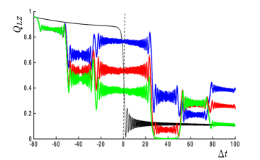
Figure 4: (Color online) Survival probability, $Q_{\scriptscriptstyle LZ}$, calculated numerically from the system Eq. (IV), is plotted versus the dimensionless time, $\Delta t$, for specific coupling strength $G=12\Delta$ and frequency $\omega=20\Delta$, so that $\frac{4G}{\omega}=2.4$ and $J_{0}(4G/\omega)=0$. Different curves correspond to the values of $\kappa$: $\kappa=\pi/2$ (blue), $\kappa=\pi/3$ (red), and $\kappa=\pi/4$ (green). It is seen that $Q_{\scriptscriptstyle LZ}$ does not change near $t=0$, where the $k=0$ LZ transition is expected suggesting that the gap is suppressed. Black line shows the time evolution of $Q_{\scriptscriptstyle LZ}$ at zero coupling. The drive velocity is $v=\pi\Delta^{2}/4$ in all the curves.

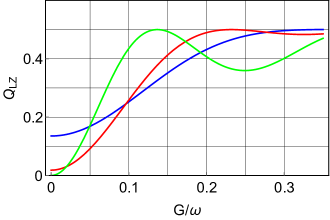
Figure 5: (Color online) The “incoherent” survival probability is plotted from Eq. (26) versus the dimensionless coupling amplitude for different values of the bare survival probability: $Q_{\scriptscriptstyle LZ}(0)=e^{-2}$ (blue), $Q_{\scriptscriptstyle LZ}(0)=e^{-4}$ (red), and $Q_{\scriptscriptstyle LZ}(0)=e^{-10}$ (green). For the latter curve the approach to the asymptote $Q_{\scriptscriptstyle LZ}(\infty)=\frac{1}{2}$ is non-monotonic.

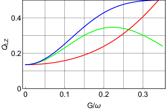
Figure 6: (Color online) Red: the survival probability, $Q_{\scriptscriptstyle LZ}^{(0)}$, is plotted from Eq. (19) versus the dimensionless coupling amplitude. The bare survival probability is chosen to be $Q_{\scriptscriptstyle LZ}(0)=e^{-2}$; Blue: the small-$G$ portion of the “incoherent” result shown in Fig. 5; Green: the dependence $Q_{\scriptscriptstyle LZ}^{(G)}$ with interference effects incorporated is plotted from Eq. (30).

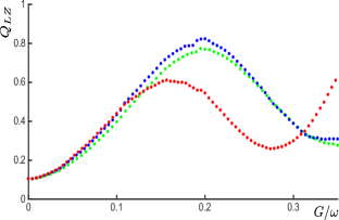
Figure 7: (Color online) The net survival probability $Q_{\scriptscriptstyle LZ}(\infty)$ calculated by solving numerically the system Eq. (IV), and subsequently averaged over $\kappa$, is plotted versus the dimensionless coupling amplitude for three values of the oscillator frequency: $\omega=20\Delta$ (green), $\omega=22\Delta$ (blue), and $\omega=23\Delta$ (red). The bare $Q_{\scriptscriptstyle LZ}$ value is chosen to be $Q_{\scriptscriptstyle LZ}=e^{-2}$, as in Fig. 4, which corresponds to the drive velocity $v=\pi\Delta^{2}/4$. In the domain $\frac{G}{\omega}<0.1$ all three curves coincide and agree with the “incoherent” and “coherent” theoretical results shown in Fig. 6. The position of the maximum also agrees with “coherent” curve in Fig. 6. However, the peak value $Q_{\scriptscriptstyle LZ}\approx 0.6$ is higher than $Q_{\scriptscriptstyle LZ}=0.35$ predicted by theory. Note that the theoretical result Eq. (30) takes into account only $k=0$ and $k=\pm 1$ intermediate transitions.

$$i\dot{\tilde{D}}_{\scriptscriptstyle 1}\left(t-\frac{\omega}{v}\right)+\frac{v}{2}\left(t-\frac{\omega}{v}\right)\tilde{D}_{\scriptscriptstyle 1}\left(t-\frac{\omega}{v}\right)\\ =\frac{\Delta}{2}\tilde{D}_{\scriptscriptstyle 2}\left(t-\frac{\omega}{v}\right)\exp\Bigg{[}i\left(\omega t-\frac{4G\sin(\omega t-\kappa)}{\omega}\right)\Bigg{]},$$ (21)

$$i\dot{\tilde{D}}_{\scriptscriptstyle 2}\left(t-\frac{\omega}{v}\right)-\frac{v}{2}\left(t-\frac{\omega}{v}\right)\tilde{D}_{\scriptscriptstyle 2}\left(t-\frac{\omega}{v}\right)\\ =\frac{\Delta}{2}\tilde{D}_{\scriptscriptstyle 1}\left(t-\frac{\omega}{v}\right)\exp\Bigg{[}-i\left(\omega t-\frac{4G\sin(\omega t-\kappa)}{\omega}\right)\Bigg{]}.$$ (22)

The same argument as above suggests that, as a result of being fast, the exponent in the right-hand side can be averaged over the period, $2\pi/\omega$, Then the system Eq. (21) will describe a regular LZ transition taking place around $t=\frac{\omega}{v}$ with a gap reduced by $J_{1}(4G/\omega)$, where $J_{1}$ is the first-order Bessel function. The corresponding survival probability reads

$$Q_{\scriptscriptstyle LZ}^{(1)}=\exp\left[-\frac{\pi\Delta^{2}}{2v}J_{1}^{2}\left(\frac{4G}{\omega}\right)\right].$$ (23)

Naturally, a similar transition taking place around
$t=-\frac{\omega}{v}$ is described by the same $Q_{\scriptscriptstyle LZ}^{(1)}$. Note also, that, in addition to $J_{1}(4G/\omega)$, the averaged matrix element is multiplied by $\exp{(i\kappa)}$. The physical meaning of the moments $t=\pm\frac{\omega}{v}$ is transparent. The energy separation between $\uparrow$ and $\downarrow$ state changes with time as $vt$. At $t=\frac{\omega}{v}$ this separation becomes equal to the oscillator quantum.

The extension of Eqs. (19), (23) to arbitrary $k$ is straightforward:

$$Q_{\scriptscriptstyle LZ}^{(k)}=\exp\left[-\frac{\pi\Delta^{2}}{2v}J_{k}^{2}\left(\frac{4G}{\omega}\right)\right].$$ (24)

The transitions taking place at $t=t_{k}$ can be viewed as well separated if the time, $\omega/v$, is much bigger than the individual LZ transition time $\sim\Delta/v$, yielding the criterion $\omega\gg\Delta$. The second condition to be met is that the effective time averaging takes place during the LZ transition time, so that $\Delta/v\gg 1/\omega$. The second condition can be cast in the form $\frac{\omega}{\Delta}\gg\frac{v}{\Delta^{2}}$. If the bare survival probability is small, $\Delta^{2}\gg v$, then the first condition is more restrictive.

Fig. 4 offers an insight into a general scenario of the LZ transition in a two-level system coupled to a fast oscillator. The system undergoes a number of individual transitions at times $t=t_{k}$ characterized by survival probabilities $Q_{\scriptscriptstyle LZ}^{(k)}$. It is also seen from Fig. 4 that the evolution of $Q_{\scriptscriptstyle LZ}$ with time depends on the wave vector, $\kappa$. This is a consequence of interference of partial transition amplitudes. To find the net survival probability analytically, we first assume that averaging over $\kappa$ suppresses the interference effects completely. Then we can write the recurrent relation for $Q_{N}$, which are the successive values of $Q_{\scriptscriptstyle LZ}$ after $N$ transitions

$$Q_{N+1}=Q_{N}\left(1-Q_{\scriptscriptstyle LZ}^{(N+1)}\right)+\left(1-Q_{N}\right)Q_{\scriptscriptstyle LZ}^{(N+1)}.$$ (25)

This relation expresses the fact that the occupation of the state $\uparrow$ after the transition comes from the occupation of this state before the transition as well as from the occupation of the state $\downarrow$ which flips in the course of the transition. It is straightforward to derive from Eq. (25) the expression for $Q_{\scriptscriptstyle LZ}$ after the arbitrary number of transitions

$$Q_{\scriptscriptstyle LZ}=\frac{1}{2}-\frac{1}{2}\prod\limits_{k}\left(1-2Q_{\scriptscriptstyle LZ}^{(k)}\right).$$ (26)

In Fig. 5 the behavior of $Q_{\scriptscriptstyle LZ}$ versus the coupling is plotted from Eq. (26) for different bare values of $Q_{\scriptscriptstyle LZ}$. Naturally, all the curves approach $1/2$ at very large coupling. This is because, at large coupling, the information about the initial state of the two-level system is erased. For the bare value $Q_{\scriptscriptstyle LZ}=e^{-2}$ the approach to $1/2$ is monotonic. However, for $Q_{\scriptscriptstyle LZ}=e^{-4}$ a wiggle emerges at $\frac{G}{\omega}\approx 0.23$. This feature evolves into a well pronounced maximum for bare $Q_{\scriptscriptstyle LZ}=e^{-10}$.

At the position of maximum in Fig. 5 (green line) the argument, $4G/\omega$, of the Bessel functions is about $0.6$. For this value and also for smaller couplings we can restrict consideration to only three LZ transitions taking place at $t=0$ and $t=\pm\omega/v$, since all higher Bessel functions are small. With only three transitions, we can incorporate the interference effects into the theory. To do so, we should take into account that each partial LZ transition is characterized by a scattering matrix which contains the survival probability and a phase, $\chi$. The evolution of the amplitudes to find the system in $\uparrow$ and $\downarrow$ states is described by the product of scattering matrices

$$M=\begin{pmatrix}\sqrt{Q_{\scriptscriptstyle LZ}^{(1)}}&-i\sqrt{1-Q_{\scriptscriptstyle LZ}^{(1)}}e^{i\chi_{\scriptscriptstyle 3}}\\ \\ \\ -i\sqrt{1-Q_{\scriptscriptstyle LZ}^{(1)}}e^{-i\chi_{\scriptscriptstyle 3}}&\sqrt{Q_{\scriptscriptstyle LZ}^{(1)}}\end{pmatrix}\begin{pmatrix}\sqrt{Q_{\scriptscriptstyle LZ}^{(0)}}&-i\sqrt{1-Q_{\scriptscriptstyle LZ}^{(0)}}e^{i\chi_{\scriptscriptstyle 2}}\\ \\ \\ -i\sqrt{1-Q_{\scriptscriptstyle LZ}^{(0)}}e^{-i\chi_{\scriptscriptstyle 2}}&\sqrt{(}Q_{\scriptscriptstyle LZ}^{(0)})\end{pmatrix}\begin{pmatrix}\sqrt{Q_{\scriptscriptstyle LZ}^{(1)}}&-i\sqrt{1-Q_{\scriptscriptstyle LZ}^{(1)}}e^{i\chi_{\scriptscriptstyle 1}}\\ \\ \\ -i\sqrt{1-Q_{\scriptscriptstyle LZ}^{(1)}}e^{-i\chi_{\scriptscriptstyle 1}}&\sqrt{Q_{\scriptscriptstyle LZ}^{(1)}}\end{pmatrix},$$ (27)

From this product one can infer the following expression for the amplitude to change the level after the three transitionsRobert

$$A_{\scriptscriptstyle\uparrow\rightarrow\downarrow}=-iQ_{\scriptscriptstyle LZ}^{(1)}\sqrt{1-Q_{\scriptscriptstyle LZ}^{(0)}}e^{-i\chi_{\scriptscriptstyle 2}}\\ -i\sqrt{Q_{\scriptscriptstyle LZ}^{(1)}Q_{\scriptscriptstyle LZ}^{(0)}(1-Q_{\scriptscriptstyle LZ}^{(1)})}\left(e^{-i\chi_{\scriptscriptstyle 1}}+e^{-i\chi_{\scriptscriptstyle 3}}\right)\\ +i(1-Q_{\scriptscriptstyle LZ}^{(1)})\sqrt{1-Q_{\scriptscriptstyle LZ}^{(0)}}e^{-i(\chi_{\scriptscriptstyle 3}-\chi_{\scriptscriptstyle 2}+\chi_{\scriptscriptstyle 1})}.$$ (28)

Different contributions to $A_{\scriptscriptstyle\uparrow\rightarrow\downarrow}$ describe partial amplitudes to change the level at one transition and to not change the level at other two transitions. The survival probability is given by $Q_{\scriptscriptstyle LZ}=1-|A_{\scriptscriptstyle\uparrow\rightarrow\downarrow}|^{2}$.

If we assume that the phases $\chi_{1}$, $\chi_{2}$, and $\chi_{3}$ are completely uncorrelated the averaging over these phases yields

$$Q_{\scriptscriptstyle LZ}^{(c)}=\left[Q_{\scriptscriptstyle LZ}^{(1)}\right]^{2}Q_{\scriptscriptstyle LZ}^{(0)}+Q_{\scriptscriptstyle LZ}^{(0)}\left[1-Q_{\scriptscriptstyle LZ}^{(1)}\right]^{2}\\ +2Q_{\scriptscriptstyle LZ}^{(1)}\left[1-Q_{\scriptscriptstyle LZ}^{(1)}\right]\left[1-Q_{\scriptscriptstyle LZ}^{(0)}\right],$$ (29)

which is nothing but the result Eq. (26) in which only the terms $k=0$ and $k=\pm 1$ are kept. Now we take into account that the transitions $k=-1$ and $k=1$ are identical, set $\chi_{1}=\chi_{3}$, and perform the averaging over the two phases. This gives

$$Q_{\scriptscriptstyle LZ}=Q_{\scriptscriptstyle LZ}^{(c)}-2Q_{\scriptscriptstyle LZ}^{(1)}Q_{\scriptscriptstyle LZ}^{(0)}\left[1-Q_{\scriptscriptstyle LZ}^{(1)}\right].$$ (30)

We note that the interference contribution to Eq. (30) is negative. In fact, it leads to a maximum in $Q_{\scriptscriptstyle LZ}(G)$ behavior even for the bare $Q_{\scriptscriptstyle LZ}=e^{-2}$, as illustrated in Fig. 6. Thus, it is the result Eq. (30) that should be compared to the numerical calculations. The results of these calculations are shown in Fig. 7, where probability, $Q_{\scriptscriptstyle LZ}$, calculated by solving the system Eq. (IV) and averaging over $\kappa$ is shown for three oscillator frequencies versus the dimensionless coupling amplitude. In the domain $\frac{G}{\omega}<0.1$ all three curves coincide and agree with the “incoherent” and “coherent” theoretical results shown in Fig. 6. The position of the maxima also agrees with the prediction of the “coherent” theory Eq. (30). However, the peak value $Q_{\scriptscriptstyle LZ}\approx 0.6$ is higher than $Q_{\scriptscriptstyle LZ}=0.35$ predicted by the theory. The possible origin of the discrepancy is that the theory Eq. (30) takes into account only $k=0$ and $k=\pm 1$ intermediate transitions. Our overall conclusion is that non-monotonic behavior of $Q_{\scriptscriptstyle LZ}(G)$ is the result of the interference of intermediate LZ transitions.

V Discussion and concluding remarks

In the present paper we focused on the question: how the longitudinal coupling to a harmonic oscillator affects the survival probability of the Landau-Zener transition in a driven two-level system.

On general grounds, one would expect the following answer to this question. Weak coupling, by making the transition less adiabatic, increases the survival probability. At very strong coupling this probability should approach $1/2$, since the memory about the initial state of the two-level system gets erased due to coupling. There is, however, the evidence that these expectations are not entirely correct. Firstly, the exact result obtained in Ref. Wubs2006++, states that, for purely longitudinal coupling, the effect is identically zero for any coupling strength. Secondly, the numerical simulations of Ref. Ashhab1, , which pertain to longitudinal coupling suggest that, at finite temperature, $Q_{\scriptscriptstyle LZ}(G)$ is a non-monotonic function with a maximum. The domain of parameters investigated in Ref. Ashhab1, is intermediate in all respects: the temperature, the oscillator frequency, and the LZ tunneling gap were of the same order. In this regime it is difficult to infer the underlying origin of this maximum.

To establish the above physical picture, we have adopted a strong assumption that the oscillator is highly excited, so that the change of the excitation level in the course of the transition is relatively small. Under this assumption, we studied the effect of coupling on the LZ transition in two limiting cases of slow and fast oscillator. For the slow oscillator our analytical results for the survival probability are given by Eqs. (14), (15), and Eq. (16). For the fast oscillator they are given by Eq. (26)and Eq. (30). We can now quantify the validity of our main assumption. For both, the slow and the fast oscillator, the LZ transition in the presence of coupling transforms into a sequence of individual transitions.Garanin2013 This is illustrated in Fig. 2b for the slow oscillator and in Fig. 4 for the fast oscillator. The number of transitions for the slow oscillator is $N_{s}=4G\omega/\pi v$. For the fast oscillator this number can be estimated by equating the argument of the Bessel function in Eq. (24) to the index, i.e. $N_{f}=4G/\omega$. Since each individual transition is associated with different level of the oscillator, the criterion that the oscillator is highly excited can be quantified as follows: the initial excitation level $n_{0}$ should be bigger than $N_{s}$ for the slow oscillator, while for the fast oscillator it should be bigger than $N_{f}$.

Although our analytical results essentially confirm the general expectations, we find that, in both limits, $Q_{\scriptscriptstyle LZ}(G)$ approaches $1/2$ with oscillations. These oscillations are the consequence of the interference of the amplitudes corresponding to different pathways through multiple LZ transitions. It is likely that non-monotonic $Q_{\scriptscriptstyle LZ}(G)$ established in Ref. Ashhab1, is the consequence of this interference.

Note finally, that throughout the paper we assumed the bare survival probability is small, so that, unlike Ref. GaraninPerturbative, , the perturbative treatment does not apply.

Acknowledgements

The work was supported by the Department of Energy, Office of Basic Energy Sciences, Grant No. DE- FG02-06ER46313.

References

- (1) A. O. Caldeira and A. J. Leggett, “Influence of Dissipation on Quantum Tunneling in Macroscopic Systems,” Phys. Rev. Lett. 46, 211 (1981).
- (2) S. Chakravarty and A. J. Leggett, “Dynamics of the Two-State System with Ohmic Dissipation,” Phys. Rev. Lett. 52, 5 (1984).
- (3) A. Leggett, S. Chakravarty, A. Dorsey, M. Fisher, A. Garg, and W. Zwerger, “Dynamics of the dissipative two-state system,” Rev. Mod. Phys. 59, 1 (1987).
- (4) L. D. Landau, “Zur theorie der energieubertragung,” Physics of the Soviet Union 2, 46 (1932).
- (5) C. Zener, “Non-adiabatic crossing of energy levels,” Proc. R. Soc. London A 137, 696 (1932).
- (6) E. Majorana, “Atomi orientati in campo magnetico vari- abile, Nuovo Cimento 9, 43 (1932).
- (7) E. C. G. Stueckelberg, “Theorie der unelastischen St osse zwischen atomen, Helv. Phys. Acta 5, 369 (1932).
- (8) Y. Gefen, E. Ben-Jacob, and A. O. Caldeira, “Zener transitions in dissipative driven systems,” Phys. Rev. B 36, 2770 (1987).
- (9) P. Ao and J. Rammer, “Quantum dynamics of a two-state system in a dissipative environment,” Phys. Rev. B 43, 5397 (1991).
- (10) E. Shimshoni and A. Stern, “Dephasing of interference in Landau-Zener transitions,” Phys. Rev. B 47, 9523 (1993).
- (11) P. Nalbach and M. Thorwart, “Landau-Zener Transitions in a Dissipative Environment: Numerically Exact Results,” Phys. Rev. Lett. 103, 220401 (2009).
- (12) S. Gasparinetti, P. Solinas, and J. P. Pekola, “Geometric Landau-Zener Interferometry,” Phys. Rev. Lett. 107, 207002 (2011).
- (13) R. S. Whitney, M. Clusel, and T. Ziman, “Temperature Can Enhance Coherent Oscillations at a Landau-Zener Transition,” Phys. Rev. Lett. 107, 210402 (2011).
- (14) C. Xu, A. Poudel, and M. G. Vavilov, “Nonadiabatic dynamics of a slowly driven dissipative two-level system,” Phys. Rev. A 89, 052102 (2014).
- (15) P. Nalbach, “Adiabatic-Markovian bath dynamics at avoided crossings,” Phys. Rev. A 90, 042112 (2014).
- (16) S. Javanbakht, P. Nalbach, and M. Thorwart, “Dissipative Landau-Zener quantum dynamics with transversal and longitudinal noise,” Phys. Rev. A 91, 052103 (2015).
- (17) M. Yamaguchi, T. Yuge, and T. Ogawa, “Markovian quantum master equation beyond adiabatic regime,” Phys. Rev. E 95, 012136 (2017).
- (18) L. Arceci, S. Barbarino, R. Fazio, G. E. Santoro, “Dissipative Landau-Zener problem and thermally assisted Quantum Annealing,” Phys. Rev. B 96, 054301 (2017).
- (19) R. K. Malla, E. G. Mishchenko, and M. E. Raikh, “Suppression of the Landau-Zener transition probability by a weak classical noise,” Phys. Rev. B 96, 075419 (2017)
- (20) M. Wubs, K. Saito, S. Kohler, Y. Kayanuma, and P. Hänggi, “Landau-Zener transitions in qubits controlled by electromagnetic fields,” New J. Phys. 7, 218 (2005).
- (21) M. Wubs, K. Saito, S. Kohler, P. Hänggi, and Y. Kayanuma, “Gauging a Quantum Heat Bath with Dissipative Landau-Zener Transitions,” Phys. Rev. Lett. 97, 200404 (2006).
- (22) K. Saito, M. Wubs, S. Kohler, P. Hänggi, and Y. Kayanuma, “Quantum state preparation in circuit QED via Landau-Zener tunneling,” Europhys. Lett. 77, 22 (2006).
- (23) K. Saito, M. Wubs, S. Kohler, Y. Kayanuma, and P. Hänggi, “Dissipative Landau-Zener transitions of a qubit: Bath-specific and universal behavior,” Phys. Rev. B 75, 214308 (2007).
- (24) D. Zueco, P. Hänggi, and S. Kohler, “Landau Zener tunnelling in dissipative circuit QED,” New J. Phys. 10, 115012 (2008).
- (25) S. Ashhab, “Landau-Zener transitions in a two-level system coupled to a finite-temperature harmonic oscillator,” Phys. Rev. A 90, 062120 (2014).
- (26) S. Ashhab, “Landau-Zener transitions in an open multilevel quantum system,” Phys. Rev. A 94, 042109 (2016).
- (27) N. A. Sinitsyn and F. Li, “Solvable multistate model of Landau-Zener transitions in cavity QED,” Phys. Rev. A 93, 063859 (2016).
- (28) C. Sun and N. A. Sinitsyn, “Landau-Zener extension of the Tavis-Cummings model: Structure of the solution,” Phys. Rev. A 94, 033808 (2016).
- (29) O. Astafiev, K. Inomata, A. O. Niskanen, T. Yamamoto, Yu. A. Pashkin, Y. Nakamura, and J. S. Tsai, “Single artificial-atom lasing,” Nature (London) 449, 588 (2007).
- (30) A. D. Cimmarusti, Z. Yan, B. D. Patterson, L. P. Corcos, L. A. Orozco, and S. Deffner, “Environment-Assisted Speed-up of the Field Evolution in Cavity Quantum Electrodynamics,” Phys. Rev. Lett. 114, 233602 (2015).
- (31) N. A. Sinitsyn, “Counterintuitive transitions in the multistate Landau-Zener problem with linear level crossings,” J. Phys. A 37, 10691 (2004).
- (32) A. V. Shytov, “Landau-Zener transitions in a multilevel system: An exact result,” Phys. Rev. A 70, 052708 (2004).
- (33) A. A. Rangelov, J. Piilo, and N. V. Vitanov, “Counterintuitive transitions between crossing energy levels,” Phys. Rev. A 72, 053404 (2005).
- (34) D. A. Garanin, R. Neb, and R. Schilling, “Effect of environmental spins on Landau-Zener transitions,” hys. Rev. B 78, 094405 (2008).
- (35) A. M. Dykhne, “Adiabatic perturbation of discrete spectrum states,” Sov. Phys. JETP 14, 941 (1962).
- (36) S. N. Shevchenko, S. Ashhab, and F. Nori, “Landau-Zener-Stückelberg interferometry,” Phys. Rep. 492, 1 (2010).
- (37) R. Glenn, M. E. Limes, B. Pankovich, B. Saam, and M. E. Raikh, “Magnetic resonance in slowly modulated longitudinal field: Modified shape of the Rabi oscillations,” Phys. Rev. B 87, 165205 (2013).
- (38) R. C. Roundy and M. E. Raikh, “Tunnel magnetoresistance in organic spin valves in the regime of multistep tunneling,” Phys. Rev. B 88, 205206 (2013).
- (39) M. F. O’Keeffe, E. M. Chudnovsky, and D. A. Garanin, “Landau-Zener dynamics of a nanoresonator containing a tunneling spin,” Phys. Rev. B 87, 174418 (2013).
- (40) D. A. Garanin and R. Schilling, “Many-body Landau-Zener effect at fast sweep,” Phys. Rev. B 71, 184414 (2005).