Fitness voter model: damped oscillations and anomalous consensus

Abstract

We study the dynamics of opinion formation in a heterogeneous voter model on a complete graph, in which each agent is endowed with an integer fitness parameter $k\geq 0$, in addition to its $+$ or $-$ opinion state. The evolution of the distribution of $k$–values and the opinion dynamics are coupled together, so as to allow the system to dynamically develop heterogeneity and memory in a simple way. When two agents with different opinions interact, their $k$–values are compared and, with probability $p$ the agent with the lower value adopts the opinion of the one with the higher value, while with probability $1-p$ the opposite happens. The winning agent then increments its $k$–value by one. We study the dynamics of the system in the entire $0\leq p\leq 1$ range and compare with the case $p=1/2$, in which opinions are decoupled from the $k$–values and the dynamics is equivalent to that of the standard voter model. When $0\leq p<1/2$, agents with higher $k$–values are less persuasive, and the system approaches exponentially fast to the consensus state of the initial majority opinion. The mean consensus time $\tau$ appears to grow logarithmically with the number of agents $N$, and it is greatly decreased relative to the linear behavior $\tau\sim N$ found in the standard voter model. When $1/2<p\leq 1$, agents with higher $k$–values are more persuasive, and the system initially relaxes to a state with an even coexistence of opinions, but eventually reaches consensus by finite-size fluctuations. The approach to the coexistence state is monotonic for $1/2<p<p_{o}\simeq 0.8$, while for $p_{o}\leq p\leq 1$ there are damped oscillations around the coexistence value. The final approach to coexistence is approximately a power law $t^{-b(p)}$ in both regimes, where the exponent $b$ increases with $p$. Also, $\tau$ increases respect to the standard voter model, although it still scales linearly with $N$. The $p=1$ case is special, with a relaxation to coexistence that scales as $t^{-2.73}$ and a consensus time that scales as $\tau\sim N^{\beta}$, with $\beta\simeq 1.45$.

I Introduction and motivation

Simple agent-based models of social interactions have attracted a lot of interest from statistical physicists in recent times. See the review Castellano et al. (2009) and the references therein. From the social sciences perspective such models can provide a controlled testing ground for more qualitative theories of social interaction. See, for example, the discussion in Macy and Willer (2002). For physicists, these models are intellectually stimulating because they exhibit a rich range of dynamical and statistical phenomena. Furthermore, as quantitative data become increasingly available, particularly from online social networks Ciulla et al. (2012) and search engine data Preis et al. (2010), there is the possibility that social modelling could become predictive Conte et al. (2012).

The statistics of consensus formation in opinion dynamics models is a problem which has proven to be particularly amenable to analysis using tools from statistical physics, such as the theory of coarsening and first-passage phenomena (see (Krapivsky et al., 2010, chap. 8)). The primary question of interest is whether the population will eventually reach consensus or a coexistence of both opinions will persist indefinitely. In principle, both outcomes are possible depending on the assumptions made about the mechanism of social influence Flache and Macy (2011). The voter model Clifford and Sudbury (1973); Holley and M. (1975); Liggett (2004) is the most basic opinion dynamics model that allows to explore the consensus problem in great detail. It is a simple interacting particle system consisting of a graph with an agent at each node possessing a single degree of freedom, its opinion $s$, taking two possible values. The dynamics is as follows: an agent is picked at random who then adopts the opinion of a randomly selected neighbour. Social influence is therefore represented as an entirely mindless process whereby agents just adopt the opinions of their neighbours at random. The model has different interpretations aside from opinion dynamics, including catalysis Krapivsky (1992) and population dynamics Clifford and Sudbury (1973). Also, different extensions of the model have been proposed in the literature, including constrained interactions Vazquez et al. (2003); Vazquez and Redner (2004), non-equivalent states Castelló et al. (2006), asymmetric transitions or bias Antal et al. (2006), noise Medeiros et al. (2006), and memory effects Dall’Asta and Castellano (2007). It is also known that several models presenting a coarsening process without surface tension belong to the voter model universality class Dornic et al. (2001); Al Hammal et al. (2005); Vazquez and López (2008).

On a finite graph, the voter model always reaches consensus by finite-size fluctuations, because the two states in which all opinions are the same are absorbing. This means that once the system randomly enters such a configuration, it stays there forever. The average time it takes a system containing $N$ agents to reach consensus is called the mean consensus time, $\tau$, which grows as $\tau\sim N^{2}$ on a regular $1D$ lattice, as $\tau\sim N\,\ln N$ on a regular $2D$ lattice, and as $\tau\sim N$ in $3D$ and above, including on the complete graph (in which every agent is connected to every other).

It is natural to ask how robust are the results described above. Research has shown that changes to the voter model, which at first sight might seem innocuous, can lead to significant changes in the statistics of consensus times. In particular, the introduction of various forms of heterogeneity can have far–reaching consequences. Heterogeneity here means that not all agents are equivalent. The introduction of even a single “zealot” Mobilia (2003) – an agent with a finite probability to unilaterally change opinion back to a preset preference – greatly increases the consensus time. Also, if all agents are assigned flip rates which are sampled from a probability distribution then, by choosing this distribution appropriately, one can make the approach to consensus arbitrarily slow Masuda et al. (2010). This model is called the Heterogeneous Voter Model. On the complete graph, one can have $\tau\sim N^{\beta}$ with $\beta>1$ arbitrarily large. This occurs because $\tau$ is dominated by the (slowest) flip rates of the “stubbornest” agents. A related model is the Partisan Voter Model Masuda et al. (2010), in which heterogeneity is introduced by randomly endowing all agents with a preferred opinion. The interaction rules are modified so that agents have a higher rate for switching to their preferred opinion. The consensus time on the complete graph was then found to be even longer and grow exponentially with $N$. In contrast to these examples, heterogeneity can also accelerate the formation of consensus. For example, if the agents acquire temporal memory such that their flip rates decrease the longer they remain in a given state then, depending on the strength of this effect, the scaling exponent of $\tau$ with $N$ decreases relative to standard voter model case Stark et al. (2008a, b). Even more extremely, if the underlying graph is replaced by a random, scale-free network, then depending on the properties of the degree distribution of this network, $\tau$ can scale sub-linearly with $N$ and can even become logarithmic or independent of $N$ Sood and Redner (2005); Suchecki et al. (2005); Vazquez and Eguíluz (2008). This effect is known as “fast consensus”. Finally, in reference Pérez et al. (2016) the authors studied a two-sate interacting particle model with age-dependent transition rates, that is, where the likelyhood that a given particle changes state depends on the time spent on its actual state. This model exhibits either dominance of old states or coexistence and synchronized collective behavior, depending on whether particles have a preference to adopt old or new states, respectively.

In this paper, we study a variant of the voter model in which, unlike the examples given above, heterogeneity is allowed to develop dynamically as a result of the interactions between agents. There are many ways in which one could imagine doing this. Our approach is one of the simplest in the sense that we have a single control parameter. Each agent is endowed with a fitness parameter, $k$, in addition to its opinion. Initially this parameter is set to zero for all agents. When two agents with different opinions interact, $k$–values are compared. Then, with probability $p$ the agent with the lower value adopts the opinion of the one with the higher value and, with the complementary probability $1-p$ the opposite happens. The winning agent then increments its $k$–value by one. This competitive aspect was motivated by the study of the evolution of competitive societies presented in Ben-Naim et al. (2006). The only parameter in the model is the probability $p$. As time passes, heterogeneity develops as a distribution of different $k$-values evolves in the population. The opinion group exchange dynamics has memory since the transition rates depend on the past history through the $k$-values, although the model can obviously be formulated in a Markovian way in the extended $(s,k)$ state space. We find that the dynamics of this model is surprisingly rich as the parameter $p$ is varied. In particular, it can exhibit both fast and slow consensus for different values of $p$, and the dynamics of the group sizes exhibits interesting oscillations in time.

The layout of the paper is as follows. In Sec. II we specify the model and explain some of the basic properties. Sec. III then presents some numerical measurements of the consensus time on a complete graph as a function of $p$ and $N$. We find that for $p>1/2$ the time to reach consensus is very large, whereas for $p<1/2$ consensus is very fast. In Sec. IV we study the rate equations for the model and discover that when $p>1/2$ the system is attracted to a coexistence state in which two equal sized populations of oppositely–opinioned agents reach a dynamic equilibrium. The approach to this state could be either monotonic or oscillatory. When $p<1/2$, the coexistence state is unstable and the system is driven quickly to consensus. We finish in Sec. VI with a short summary and conclusions.

II Definition of the model

Two groups, labeled ($\pm$), compete for membership in a population of $N$ agents. The interaction network is a complete graph so any agent can interact with any other. In addition to its group designation, or opinion $s=\pm$, each agent has an integer fitness $k$. In a single time step $\Delta t=2/N$, two agents are selected at random. If both have the same opinion nothing happens. If not, they interact as follows. Agents compare their respective $k$–values. With probability $p$, the agent with the lower $k$–value adopts the opinion of the agent with the higher value. With probability $1-p$, the opposite happens and the agent with the higher $k$–value adopts the opinion of the agent with the lower value. If both $k$–values are equal then one agent adopts the opinion of the other with equal probability $1/2$. The “winning” agent (i.e. the one whose opinion remained unchanged) then increments its $k$–value by one. Assuming that the chosen agents have opinions $s_{1}$ and $s_{2}$ (with $s_{1}\neq s_{2}$), and fitness $k_{1}$ and $k_{2}$, the interaction rules can be summarized schematically as:

If $k_{1}>k_{2}$ then

$$(s_{1},k_{1})\oplus(s_{2},k_{2}) \rightarrow \left\{\begin{array}[]{ll}(s_{1},k_{1}+1)\oplus(s_{1},k_{2})&\mbox{Prob. $p$}\\ (s_{2},k_{1})\oplus(s_{2},k_{2}+1)&\mbox{Prob. $1-p$}.\end{array}\right.$$ (3)

If $k_{1}=k_{2}=k$ then

$$(s_{1},k)\oplus(s_{2},k) \rightarrow \left\{\begin{array}[]{ll}(s_{1},k+1)\oplus(s_{1},k)&\hskip 8.82028pt\mbox{Prob. $1/2$}\\ (s_{2},k)\oplus(s_{2},k+1)&\hskip 8.82028pt\mbox{Prob. $1/2$}.\end{array}\right.$$ (6)

The only parameter in this model is the probability $p$. When $p=1/2$, the $k$–values of the agents play no role in the opinion dynamics since each agent has a 50–50 chance of adopting the opinion of the other. Thus for $p=1/2$, the evolution of the $k$–values decouple from the opinion dynamics which is therefore equivalent to the standard voter model. If $p>1/2$, a higher value of $k$ makes an agent less likely to change opinion during an interaction. Thus, in this regime, one could interpret the above rules as saying that agents become more confident of their opinion each time they succeed in convincing other agents to switch groups. As $p$ gets close to one, agents which reach high $k$–values become highly unlikely to change their opinion. Thus “zealots” emerge dynamically in this model. If $p<1/2$, the opposite is true: agents with high $k$–values are more likely to change opinion frequently.

III Consensus times

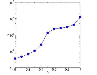
Figure 1: Linear-log plot of the mean consensus time $\tau$ vs the probability $p$ that the fitter agent wins in an interaction, for a system of $N=1000$ agents.

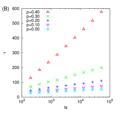
Figure 2: (A) Mean consensus time $\tau$ as a function of the number of agents $N$ on a log-log scale, for $p$ in the range $\frac{1}{2}\leq p\leq 1$. Upper and lower straight lines have slope $1.45$ and $1.0$, respectively. Inset: $\tau$ is compensated by $N$. The horizontal line is the prefactor $2\ln(2)$ of the standard voter model ($p=1/2$). (B) $\tau$ vs $N$ on a log-linear scale for $0\leq p<\frac{1}{2}$.

We performed Monte Carlo simulations of the dynamics defined in Sec. II above on complete graphs of various sizes $N$ and for several values of $p$ in the interval $[0,1]$, and measured the time to reach opinion consensus. Initially, each agent takes opinion $+$ or $-$ with the same probability $1/2$, and all agents have fitness $k=0$. Results are shown in Figs. 1 and 2. As discussed above, the basis for comparison is the $p=1/2$ case where the opinion dynamics is equivalent to the standard voter model for which the consensus time scales as $\tau=2\ln(2)N$ on the complete graph, when the initial state consists on $N/2$ agents in each opinion state.

In Fig. 1 we plot the mean consensus time $\tau$ measured from simulations, as a function of the probability $p$. The average was done over $10^{4}$ independent realizations of the dynamics. We observe that $\tau$ increases rapidly with $p$, and becomes very large when $p$ overcomes the value $1/2$. This is an indication that the behaviour for $p>1/2$ is strikingly different from that of $p<1/2$. Figure 2(A) shows $\tau$ as a function of $N$ for a range of values of $p$ between $1/2$ and $1$. With the exception of the curve for $p=1$, all curves grow as $N$ for large $N$ (lower straight line). This can be seen in the inset of Fig. 2(A), where $\tau$ is compensated by $N$. All curves for $p<1$ reach a plateau as $N$ grows, although the saturation level increases with $p$. Thus, the consensus time grows with $p$ although it still scales linearly with $N$ as in the standard voter model. The case $p=1$ seems quantitatively different. A closer analysis of the data indicates that for $p=1$, $\tau\sim N^{\beta}$ with $\beta\simeq 1.45$ (upper straight line). Simulations with values of $p$ very close to $1$ (see $p=0.99$ curve) suggest that the case $p=1$ really is uniquely different. As best as we have been able to tell from the numerics, the scaling exponent jumps at $p=1$. As we see in Fig. 2(B), the behaviour of $\tau$ for $p<1/2$ is quite different. We observe that $\tau$ grows very slowly with the system size, as $\tau\sim\ln N$, indicating that the system goes to a “fast consensus”.

In summary, the consensus is slow for $p\geq 1/2$ and very fast for $p<1/2$. In an attempt to get some insight into these behaviours, we shall now study the rate equations corresponding to this model.

IV Mean field dynamics

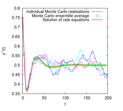
Figure 3: Comparison between the evolution of $\rho_{+}(t)$ obtained from the numerical solution of Eqs. (7) (solid line) with that obtained from an ensemble average of $1000$ Monte Carlo realizations (circles) of the stochastic process described in Sec. II with $N=6400$ agents. The value of $p$ is $1.0$ and the initial condition is $\rho_{+}(0)=0.75$. Three different individual realizations of the stochastic dynamics are also shown in dashed lines.

IV.1 Rate equations

Let us now write down the mean-field (MF) rate equations for the stochastic dynamics described in Sec. II. Adopting some of the notation from Ben-Naim et al. (2006), the time evolution of the fraction of agents with opinion $+$ and fitness $k$, $f_{k}^{+}$, is given by

$$\frac{d{f}^{+}_{k}}{dt} = p\,\left(f_{k\!-\!1}^{+}F_{k\!-\!1}^{-}-f_{k}^{+}F_{k}^{-}\right)+(1\!-\!p)\,\left(f_{k\!-\!1}^{+}G_{k\!-\!1}^{-}-f_{k}^{+}G_{k}^{-}\right)$$ (7)

$$+ p\,\left(f_{k}^{-}G_{k}^{+}-f_{k}^{+}G_{k}^{-}\right)+(1\!-\!p)\,\left(f_{k}^{-}F_{k}^{+}-f_{k}^{+}F_{k}^{-}\right)$$

$$+ \frac{1}{2}\left(f_{k\!-\!1}^{+}f_{k\!-\!1}^{-}-f_{k}^{+}f_{k}^{-}\right),$$

$$\frac{d{f}^{-}_{k}}{dt} = \left[+\leftrightarrow-\right],$$

where

$$F_{k}^{\pm}=\sum_{i=0}^{k-1}f_{i}^{\pm}\mbox{\ \ \ and \ \ \ }G_{k}^{\pm}=\sum_{i=k+1}^{\infty}f_{i}^{\pm}.$$ (8)

The corresponding equation for $f_{k}^{-}$ is obtained by switching the $+$ and $-$ labels in Eq. (7). This occurs frequently in the analysis which follows. For the sake of conciseness, we shall not explicitly write out the symmetric partner of each equation unless it is necessary. All terms appear in pair of positive and negative terms describing the gain and loss of agents having opinion $+$ and $k$–value, $k$. The first pair of terms accounts for interactions of $+$ agents with $-$ agents having a lower $k$–value, with the result that the original agent remains $+$. The second pair of terms accounts for interactions of $+$ agents with $-$ agents having a higher $k$–value, with the result that the original agent remains $+$. The third pair of terms accounts for the interactions of $-$ agents with $+$ agents having a higher $k$–value, with the result that the original agent switches opinion to $+$. The fourth pair of terms accounts for the interactions of $-$ agents with $+$ agents having a lower $k$–value, with the result that the original agent switches opinion to $+$. The final pair of terms accounts for the cases when two interacting agents have equal $k$–values.

The fraction of the total population in each group is

$$\rho_{\pm}(t)=\sum_{k=0}^{\infty}f_{k}^{\pm}.$$ (9)

The mean $k$–value of each group is

$$\mu_{\pm}(t)=\sum_{k=0}^{\infty}k\,f_{k}^{\pm}.$$ (10)

Since $f^{\pm}_{k}$ are proportions, we must have $\rho_{+}(t)+\rho_{-}(t)=1$. We shall denote the mean $k$–value across the entire population by $\mu(t)=\mu_{+}(t)+\mu_{-}(t)$. By summing Eqs. (7) over $k$, we obtain the following equations for the populations of each group:

$$\frac{d\rho_{+}}{dt} = (2p-1)\,\sum_{k=0}^{\infty}\left(f_{k}^{+}F_{k}^{-}-f_{k}^{-}F_{k}^{+}\right),$$

$$\frac{d\rho_{-}}{dt} = \left[+\leftrightarrow-\right].$$ (11)

It is clear from these formulae that the sum of the populations is conserved. Furthermore, when $p=\frac{1}{2}$ we see that the two populations are conserved individually. This is to be expected since for $p=\frac{1}{2}$ the dynamics of the $k$–counter is entirely decoupled from the dynamics of exchange between the two opinion groups. Then, the competition between the groups is described by the simple voter model, for which we know that the individual populations are conserved on average. By multiplying Eqs. (7) by $k$ and summing over $k$, we obtain the following less elegant equations for the mean $k$–value of each group:

$$\frac{d\mu_{+}}{dt} = (1-p)\,\rho_{+}\rho_{-}+p\,\left(\rho_{+}\mu_{-}-\rho_{-}\mu_{+}\right)$$

$$+(2p\!-\!1)\sum_{k=0}^{\infty}k\,\left(f_{k}^{+}F_{k}^{-}-f_{k}^{-}F_{k}^{+}\right)$$

$$+(2p\!-\!1)\sum_{k=0}^{\infty}f_{k}^{+}F_{k}^{-}+\frac{1}{2}(2p\!-\!1)\sum_{k=0}^{\infty}f_{k}^{+}f_{k}^{-},$$

$$\frac{d\mu_{-}}{dt} = \left[+\leftrightarrow-\right].$$ (12)

The average $k$–value of the whole population satisfies

$$\frac{d\mu}{dt} = (2p-1)\sum_{k=0}^{\infty}\left(f_{k}^{+}F_{k}^{-}+\frac{1}{2}f_{k}^{+}f_{k}^{-}+f_{k}^{-}F_{k}^{+}\right)$$ (13)

$$+2(1-p)\,\rho_{+}\rho_{-}$$

$$= \rho_{+}\,\rho_{-},$$

where some careful algebra is required to establish simplify the sums. Equation (13) shows that the mean of the total fitness grows at a rate $\rho_{+}\rho_{-}$, which is time dependent. This equation can also be derived by considering the mean change of $\mu$, $\Delta\mu$, in a single time step $\Delta t=2/N$ of the dynamics. An update occurs only when a $+$ and a $-$ agents are chosen, which happens with probability $2\rho_{+}\rho_{-}$. Then, one of the agents increases its fitness by one, changing $\mu$ by $1/N$ ($\Delta\mu=1/N$). Then we can write

$$\frac{d\mu}{dt}\simeq\frac{\Delta\mu}{\Delta t}=\frac{2\rho_{+}\rho_{-}(\frac{1}{N})}{2/N}=\rho_{+}\rho_{-},$$ (14)

as in Eq. (13). It is difficult to tell a-priori how the total $k$–value in the system will behave since it depends on the fraction of the population in the two groups. We note, however, that when $p=1/2$, $\mu(t)$ grows linearly since $\rho_{\pm}$ are constant and given by their initial values. We can also check that for $p=1/2$ and initial densities $\rho_{+}(0)=3/4$ and $\rho_{-}(0)=1/4$, Eqs. (12) are reduced to

$$\frac{d\mu_{+}}{dt} = \frac{3}{32}+\frac{1}{8}(3\mu_{-}-\mu_{+}),$$

$$\frac{d\mu_{-}}{dt} = \frac{3}{32}-\frac{1}{8}(3\mu_{-}-\mu_{+}),$$

whose solutions with initial mean $k$–values $\mu_{+}(0)=\mu_{-}(0)=0$ are

$$\mu_{+}(t) = \frac{3}{32}\left(\frac{3}{2}t+e^{-t/2}-1\right),$$

$$\mu_{-}(t) = \frac{3}{32}\left(\frac{1}{2}t-e^{-t/2}+1\right).$$ (15)

Equations (15) show that the mean $k$–values increase linearly at large times, as $\mu_{+}(t)\simeq 9t/64$ and $\mu_{-}(t)\simeq 3t/64$, as we can also see in the inset of Fig. 5(A).

IV.2 Numerical solutions of the rate equations

On a complete graph, Eqs. (7) exactly describe the ensemble averaged behaviour of the system. This is illustrated in Fig. 3 which compares the evolution of $\rho_{+}(t)$ (solid line) obtained from a numerical solution of Eqs. (7) with the evolution of the ensemble average of $\rho_{+}(t)$ (circles) obtained from $1000$ realisations of the stochastic model described in Sec. II. Results correspond to $p=1.0$ and initial condition $\rho_{+}(0)=0.75$. Two features of the dynamics are striking. Firstly, we notice that starting from an asymmetric initial state that favors the $+$ opinion group ($\rho_{+}(0)=0.75$ and $\rho_{-}(0)=0.25$), the dynamics drives the system towards a coexistence state composed by even fractions of agents with $+$ and $-$ opinions ($\rho_{+}(t)=\rho_{-}(t)=1/2$). Secondly, we notice that the approach to the coexistence state is not monotonic: the dynamics have a damped oscillatory character. This suggests that the state in which both populations are equal is a fixed point. Figure 3 also shows three independent realisations (dashed lines), as compared to the ensamble average. This illustrates the importance of fluctuations which are ultimately responsible for the system reaching consensus as found in Sec. III, despite the fact that the dynamics drives the system towards coexistence.

${\mathbf{p}=\frac{1}{4}}$

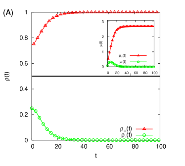
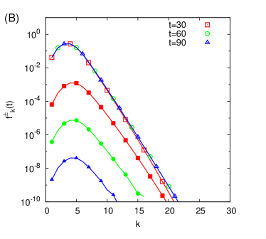
Figure 4: (Color online) MF dynamics from Eqs. (7) for $p=1/4$. (A) Time evolution of the fraction of agents in the two opinion groups $\rho_{\pm}(t)$. Inset: Evolution of the mean fitness values $\mu_{\pm}(t)$. (B) Snapshots of the $k$–value distributions $f_{k}^{+}$ (empty symbols) and $f_{k}^{-}$ (filled symbols) at different times.

${\mathbf{p}=\frac{1}{2}}$

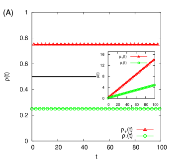
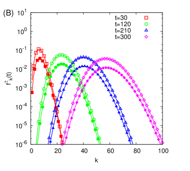
Figure 5: (Color online) MF dynamics from Eqs. (7) for $p=1/2$. (A) Time evolution of the fraction of agents in the two opinion groups $\rho_{\pm}(t)$. Inset: Evolution of the mean fitness values $\mu_{\pm}(t)$. (B) Snapshots of the $k$–value distributions $f_{k}^{+}$ (empty symbols) and $f_{k}^{-}$ (filled symbols) at different times.

${\mathbf{p}=\frac{3}{4}}$

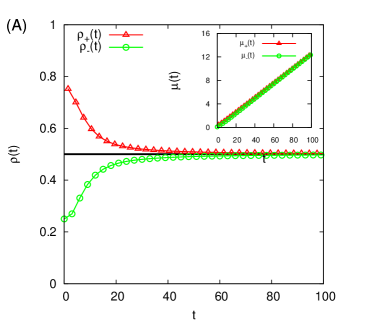
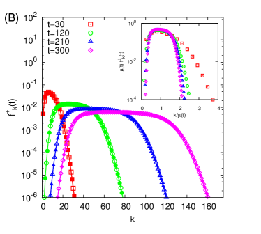
Figure 6: (Color online) MF dynamics from Eqs. (7) for $p=3/4$. (A) Time evolution of the fraction of agents in the two opinion groups $\rho_{\pm}(t)$. Inset: Evolution of the mean fitness values $\mu_{\pm}(t)$. (B) Snapshots of the $k$–value distributions $f_{k}^{+}$ (empty symbols) and $f_{k}^{-}$ (filled symbols) at different times. The inset shows the collapse of the data obtained from the self-similar scaling, Eq. (20).

${\mathbf{p}=1}$

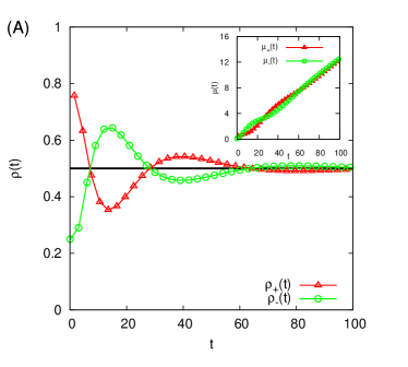
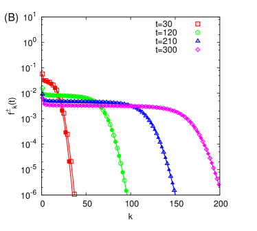
Figure 7: (Color online) MF dynamics from Eqs. (7) for $p=1$. (A) Time evolution of the fraction of agents in the two opinion groups $\rho_{\pm}(t)$. Inset: Evolution of the mean fitness values $\mu_{\pm}(t)$. (B) Snapshots of the $k$–value distributions $f_{k}^{+}$ (empty symbols) and $f_{k}^{-}$ (filled symbols) at different times.

In Figs. 4–7 we explore the behaviour of the system by means of Eqs. 7 in the entire range of $p$ values: $p=1/4$ (Fig. 4), $p=1/2$ (Fig. 5), $p=3/4$ (Fig. 6) and $p=1$ (Fig. 7). Figures 4(A)–7(A) show the time evolution of $\rho_{\pm}(t)$, while their insets show the dynamics of $\mu_{\pm}(t)$. Figures 4(B)–7(B) show snapshots at various times of the corresponding $k$–value distributions, $f^{\pm}_{k}(t)$. In Fig. 4 we see that for $p=1/4$ the system quickly reaches consensus in the opinion of the initial majority, as $\rho_{+}$ approaches exponentially fast to $1.0$. This is in agreement with the fast consensus observed in Fig. 2(B) for $p<1/2$. Thus, the dynamics for $p<1/2$ favors the opinion state of the majority, creating a positive feedback in which the largest opinion group permanently increases while the smallest group shrinks and eventually disappear. This can also be seen in Fig. 4(B), where $f^{-}_{k}(t)$ vanishes for long times (filled symbols). Figure 5(A) shows that the fractions $\rho_{\pm}$ are conserved for $p=1/2$, and that the mean $k$–values $\mu_{\pm}$ grow linearly with time, as discussed in Sec. IV.1. For both $p=3/4$ and $p=1$ the system quickly relaxes to the coexistence state $\rho_{+}=\rho_{-}=1/2$, but in different ways. Whereas for $p=3/4$ densities $\rho_{\pm}$ decay monotonically towards the value $1/2$, for $p=1$ the approach to coexistence exhibits damped oscillations. Finite-size fluctuations –not captured by the MF equations– eventually drive the system from the coexistence state to consensus, which leads to the very long consensus times measured for $p>1/2$ [see Fig. 2(A)].

IV.3 $p>\frac{1}{2}$ : Self-similar solution for the coexistence state

The above argument requires that for $p>1/2$ the large time solution of Eqs. (7) converge to a coexistence state in which both populations have the same fraction of agents ($\rho_{+}=\rho_{-}$) and equivalent $k$–value distributions, as we can see in Figs. 6 and 7. In this section we demonstrate the existence of a self-similar solution of Eqs. (7) which achieve this. Substituting $f_{k}^{+}(t)=f_{k}^{-}(t)=f_{k}(t)$ in these equations and simplifying gives:

$$\frac{d}{dt}{f}_{k} =p\left(f_{k-1}F_{k-1}-f_{k}F_{k}\right)+(1-p)\left(f_{k-1}G_{k-1}-f_{k}G_{k}\right)$$

$$+\frac{1}{2}\left(f_{k-1}^{2}-f_{k}^{2}\right).$$ (16)

Following Ben–Naim et al. Ben-Naim et al. (2006) we rewrite this equation using $f_{k}=F_{k+1}-F_{k}$ and $G_{k}=F_{\infty}-F_{k+1}=1/2-F_{k+1}$ (where the maximum group size is $\rho_{+}=F^{+}_{\infty}=1/2$ or $\rho_{-}=F^{-}_{\infty}=1/2$). This gives a closed equation for the cumulative distribution:

$$\frac{d}{dt}{F}_{k} =pF_{k-1}(F_{k-1}-F_{k})-\frac{1}{2}\left(F_{k}-F_{k-1}\right)^{2}$$

$$+(1-p)(1/2-F_{k})(F_{k-1}-F_{k}).$$ (17)

The boundary conditions are $F_{0}=0$ and $F_{\infty}=1/2$. Taking the continuum limit of Eq. (17) and keeping only the leading order term, we get

$$\frac{\partial F}{\partial t}=\left[\frac{1}{2}(p-1)+(1-2p)F\right]\frac{\partial F}{\partial k}.$$ (18)

We have observed already that $\mu_{\pm}(t)$ grows linearly for large times when $p>1/2$, thus the mean value of the distributions

$$\langle k\rangle^{\pm}=\frac{1}{\rho_{\pm}}\sum_{k=0}^{\infty}k\,f_{k}^{\pm}=\frac{\mu_{\pm}}{\rho_{\pm}}=2\mu_{\pm}=\mu$$

also increase linearly with time. This suggests that we look for solutions of Eq. (18) in which the cumulative distribution, $F(k,t)$, has the scaling form:

$$F(k,t)\simeq\Phi(\xi)\hskip 14.22636pt\mbox{with $\xi\equiv\frac{k}{\mu(t)}=\frac{k}{\alpha t}$},$$ (19)

where $\alpha\simeq 0.24$ is twice the slope of the $\mu_{\pm}$ vs $t$ curves for $t>60$ in the inset of Figs. 6 and 7. This is equivalent to the following self-similar form for the $k$–value distribution itself

$$f^{\pm}_{k}(t)\simeq\mu(t)^{-1}\,\phi(\xi)\hskip 14.22636pt\mbox{where $\varphi\equiv\frac{d\Phi}{d\xi}$.}$$ (20)

In the scaling variables, Eq. (18) takes the form

$$\left[\frac{1}{2}(p-1)+\alpha\,\xi+(1-2p)\Phi(\xi)\right]\frac{d\Phi}{d\xi}=0,$$ (21)

Solving Eq. (21) gives

$$\Phi(\xi)=\mathrm{constant}\hskip 14.22636pt\mbox{or}\hskip 14.22636pt\Phi(\xi)=\frac{\frac{1}{2}(p-1)}{2p-1}+\frac{\alpha\,\xi}{2p-1}.$$

Following Ben-Naim et al. (2006), we use the boundary conditions $\Phi(0)=0$ and $\Phi(\infty)=1/2$, the monotonicity of $F_{k}$, $d\Phi/d\xi\geq 0$, and the bounds $0\leq\Phi\leq 1$, to assemble a sensible piece-wise smooth solution:

$$\Phi(\xi)=\begin{cases}0&\mbox{if $0<\xi<\xi_{-}$}\\ \frac{\frac{1}{2}(p-1)}{2p-1}+\frac{\alpha\,\xi}{2p-1}&\mbox{if $\xi_{-}<\xi<\xi_{+}$}\\ 1/2&\mbox{if $\xi_{+}<\xi$,}\end{cases}$$ (22)

where $\xi_{-}=(1-p)/2\alpha$ and $\xi_{+}=p/2\alpha$. We remark that if we keep the next order (diffusive) terms in the derivation of Eq. (18), then the sharp corners in this solution would be smoothed out. Differentiating this solution with respect to $\xi$ gives the corresponding scaling function for the $k$–value distribution itself [see Eq. (20)]

$$\mu(t)f_{k}^{\pm}(t)=\phi(\xi)=\begin{cases}0&\mbox{if $0<\xi<\xi_{-}$}\\ \frac{\alpha}{2p-1}&\mbox{if $\xi_{-}<\xi<\xi_{+}$}\\ 0&\mbox{if $\xi_{+}<\xi$,}\end{cases}$$ (23)

where $\xi_{\pm}$ are the same as in Eq. (22) above. Note that as $p\to 1/2$, this solution tends to a $\delta$-function. This case will be considered in the next section. The inset of Figs. 6(B) and 7(B) shows the data collapse of some snapshots of the full $k$–value distributions obtained from numerics (symbols) onto the curve given by Eq. (23) (solid line).

IV.4 $p=\frac{1}{2}$: Dynamics of $k$–value distribution

For completeness, let us look at what happens on the boundary when $p=1/2$. Many of the terms in Eqs. (7) are then absent due to the fact that $F_{k}^{\pm}(t)+f_{k}^{\pm}(t)+G_{k}^{\pm}(t)=\rho_{\pm}(t)$. Further simplification follows from Eq. (11) which tells us that $\rho_{\pm}(t)$ are constant when $p=1/2$. This reflects the fact that the evolution of the distribution of $k$–values decouples from the opinion dynamics which are equivalent to the standard voter model dynamics in which the average magnetization is conserved. Eqs. (7) become

$$\frac{\partial f^{+}_{k}}{\partial t} = \frac{1}{2}\rho_{-}\left(f_{k-1}^{+}-f_{k}^{+}\right)+\rho_{+}f_{k}^{-}-\rho_{-}f_{k}^{+}$$

$$\frac{\partial f^{-}_{k}}{\partial t} = \left[+\leftrightarrow-\right].$$

Taking the continuum limit we get

$$\frac{\partial f^{+}_{k}}{\partial t} = -\frac{1}{2}\rho_{-}\frac{\partial f_{k}^{+}}{\partial k}+\frac{1}{4}\rho_{-}\frac{\partial^{2}f_{k}^{+}}{\partial k^{2}}-\rho_{-}f_{k}^{+}+\rho_{+}f_{k}^{-}$$

$$\frac{\partial f^{-}_{k}}{\partial t} = \left[+\leftrightarrow-\right].$$ (24)

The initial conditions are $f_{k}^{\pm}=\rho_{\pm}\,\delta(k)$. We should also impose the zero-flux boundary conditions, $\frac{\partial f_{k}^{\pm}}{\partial k}=0$ at $k=0$ since the $k$–values cannot become negative. Eqs. (24) are a pair of coupled linear equations which can be decoupled and solved in Fourier-space. The symmetric case $\rho_{+}=\rho_{-}=1/2$ is particularly simple and illustrative, in which both distributions are identical and evolve according to the single advection-diffusion equation,

$$\frac{\partial f^{\pm}}{\partial t}=-\frac{1}{4}\frac{\partial f^{\pm}}{\partial k}+\frac{1}{8}\frac{\partial^{2}f^{\pm}}{\partial k^{2}}.$$ (25)

The solution of this equation on the whole of $\mathbb{R}$ is

$$f^{\pm}(k,t)={\sqrt{\frac{2}{\pi t}}}\,\mathrm{e}^{-\frac{2\,(k-t/4)^{2}}{t}}.$$

In order to satisfy the boundary condition at $k=0$ we can employ the method of images to obtain

$$f^{\pm}(k,t)=\frac{1}{2}\sqrt{\frac{2}{\pi t}}\,\left(\mathrm{e}^{-\frac{2\,(k-t/4)^{2}}{t}}+\mathrm{e}^{-\frac{2\,(k+t/4)^{2}}{t}}\right).$$ (26)

We see that the $k$–value distribution is a Gaussian which propagates to the larger values of $k$ with fixed speed $v=1/4$, and whose width increases with time as $\sigma=\sqrt{t}/2$. This remains true, although it is more difficult to show analytically if $\rho_{+}\neq\rho_{-}$ [see Fig. 5(B)]. Note that by including the higher order derivative in taking the continuous limit in Eq. (24), the singular behaviour of the scaling solution, Eq. (23), is regularized.

V A reduced model of the dynamics

In order to better understand the dynamics described in Sec. IV, we introduce a reduced model which captures most of the essential features of Eqs. (7) but is simple enough to allow some insight to be obtained. If we think of the $f_{k}^{\pm}$ as being analogous to probability distributions, then their specification is equivalent to the specification of all their moments. We have already seen, however, that even the first two moments, $\rho^{\pm}$ and $\mu^{\pm}$, satisfy complicated equations, Eqs. (11) and (12) involving cross-correlations between $f_{k}^{+}$ and $f_{k}^{-}$. In principle, one could use the dynamical equations to write evolution equations for these cross-correlations but such equations would involve triple correlations and so on. Such an approach is unlikely to lead anywhere. Instead, in the spirit of moment closures and single point closures in turbulence, we suggest to close the system at the level of the first order (in $f_{k}^{\pm}$) quantities $\rho^{\pm}$ and $\mu_{\pm}$. That is to say, we attempt to ”approximate” the RHS of Eqs. (11) and (12) with functions of $\rho_{\pm}$ and $\mu_{\pm}$ only. This would yield a simple three dimensional dynamical system (not four dimensional because $\rho_{+}+\rho_{-}=1$) in place of the infinite hierarchy of equations in (7). Of course, this cannot be done exactly and the trick in obtaining useful closures is to come up with a reasonable proposal for these functions should be.

Inspired by the $k$–value distributions in Fig. 6(C) and aiming to build the simplest possible model, we introduce the following model for the $k$–value distributions:

$$\widetilde{f}_{k}^{\pm}=\frac{\rho_{\pm}^{2}}{2\mu_{\pm}}\,\,\Theta(k)\,\Theta\left(\frac{2\mu_{\pm}}{\rho_{\pm}}-k\right),$$ (27)

where $\Theta(x)$ is the Heaviside theta function. We therefore treat the distributions $f_{k}^{\pm}$ as being uniform on an interval $\left[0,K\right]$. The width, $K$, of this interval and the value of the function on the interval are chosen such that we have the following properties:

$$\int_{0}^{\infty}\widetilde{f}_{k}^{\pm}\,dk = \rho_{\pm}$$

$$\int_{0}^{\infty}k\,\widetilde{f}_{k}^{\pm}\,dk = \mu_{\pm},$$

where, in order to simplify things, we shall treat the $k$–value as a continuous variable from this point on. We can now integrate Eq. (27) to get a model for the cumulative distribution, $F_{k}^{\pm}$:

$$\widetilde{F}_{k}^{\pm}=\begin{cases}\frac{\rho_{\pm}^{2}}{2\mu_{\pm}}k&\mbox{if $0\leq k\leq\frac{2\mu_{\pm}}{\rho_{\pm}}$},\\ \rho_{\pm}&\mbox{if $k\geq\frac{2\mu_{\pm}}{\rho_{\pm}}$.}\end{cases}$$ (28)

We now substitute Eqs. (27) and (28) into Eqs. (11) and (12) and perform the integrations on the RHS in order to obtain expressions which depend only on $\rho_{\pm}$ and $\mu_{\pm}$. This is a surprisingly tedious process given the deceptive simplicity of Eq. (27). Using Mathematica and massaging the output a little, we obtained the following dynamical system

$$\frac{d\rho_{+}}{dt} =(2p-1)\,R^{+}_{1},$$ (29a)

$$\frac{d\rho_{-}}{dt} =\left[+\leftrightarrow-\right],$$ (29b)

$$\frac{d\mu_{+}}{dt} =(1-p)\,\rho_{+}\rho_{-}+p\,\left(\rho_{+}\mu_{-}-\rho_{-}\mu_{+}\right)$$

$$+(2p\!-\!1)\left(R^{+}_{2}+R^{+}_{3}+R^{+}_{4}\right),$$ (29c)

$$\frac{d\mu_{-}}{dt} =\left[+\leftrightarrow-\right],$$ (29d)

where

$$R^{+}_{1} =\int_{0}^{\infty}\left(\widetilde{f}_{k}^{+}\widetilde{F}_{k}^{-}-\widetilde{f}_{k}^{-}\widetilde{F}_{k}^{+}\right)\,dk$$ (30a)

$$=\left(\mu_{+}\rho_{-}-\mu_{-}\rho_{+}\right)R^{+},$$

$$R^{+}_{2} =\int_{0}^{\infty}k\,\left(\widetilde{f}_{k}^{+}\widetilde{F}_{k}^{-}-\widetilde{f}_{k}^{-}\widetilde{F}_{k}^{+}\right)\,dk$$ (30b)

$$=\frac{\left(\mu_{+}^{2}\rho_{-}^{2}-\mu_{-}^{2}\rho_{+}^{2}\right)R^{+}}{\rho_{+}\rho_{-}},$$

$$R^{+}_{3} =\int_{0}^{\infty}\widetilde{f}_{k}^{+}\widetilde{F}_{k}^{-}\,dk$$ (30c)

$$=\frac{1}{4\mu_{+}\mu_{-}}\Big{\{}2\mu_{+}^{2}\rho_{-}^{2}$$

$$-\left(\mu_{+}\rho_{-}-\mu_{-}\rho_{+}\right)\left[\left(\mu_{+}\rho_{-}-\mu_{-}\rho_{+}\right)+|\mu_{+}\rho_{-}-\mu_{-}\rho_{+}|\right]\Big{\}},$$

$$R^{+}_{4} =\frac{1}{2}\int_{0}^{\infty}\widetilde{f}_{k}^{+}\widetilde{f}_{k}^{-}\,dk=\frac{\rho_{+}\rho_{-}R^{+}}{4},$$ (30d)

with

$$R^{+}=\frac{1}{2\mu_{+}\mu_{-}}\left[\left(\mu_{+}\rho_{-}+\mu_{-}\rho_{+}\right)-|\mu_{+}\rho_{-}-\mu_{-}\rho_{+}|\right].$$ (31)

When performing the integrals we considered separately the two cases $\mu_{+}\rho_{-}>\mu_{-}\rho_{+}$ and $\mu_{+}\rho_{-}<\mu_{-}\rho_{+}$, which leaded to expressions defined by parts. Then, we used the absolute value function $|\bullet|$ to rewrite these expressions. For instance

$$R^{+}_{4}=\begin{cases}R^{+}_{a}&\mbox{if $\mu_{+}\rho_{-}>\mu_{-}\rho_{+}$},\\ R^{+}_{b}&\mbox{if $\mu_{+}\rho_{-}<\mu_{-}\rho_{+}$,}\end{cases}$$ (32)

with $R^{+}_{a}=\rho_{+}^{2}\rho_{-}/4\mu_{+}$ and $R^{+}_{b}=\rho_{+}\rho_{-}^{2}/4\mu_{-}$, was rewritten as

$$R^{+}_{4}=\frac{(R^{+}_{a}+R^{+}_{b})}{2}+\frac{(R^{+}_{a}-R^{+}_{b})}{2}\frac{|\mu_{+}\rho_{-}-\mu_{-}\rho_{+}|}{(\mu_{+}\rho_{-}-\rho_{-}\mu_{+})},$$

which is reduced to Eq. (30d) after some algebra.

This reduced model reproduces all the qualitative features of the full MF equations, (7). In particular, the absorbing states in Eqs. (7) correspond to lines of fixed points in the reduced model. We refer to these as the $+$ and $-$ consensus fixed points $P_{+}$ and $P_{-}$. They are parameterized by a single parameter, $\mu>0$:

$$P_{+} : (\rho_{+},\rho_{-},\mu_{+},\mu_{-})=(1,0,\mu,0)$$

$$P_{-} : (\rho_{+},\rho_{-},\mu_{+},\mu_{-})=(0,1,0,\mu).$$

That these points are zeroes of the right-hand side of Eqs. (29)–(31) for any value of $\mu$ can be verified by direct substitution.

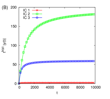
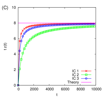
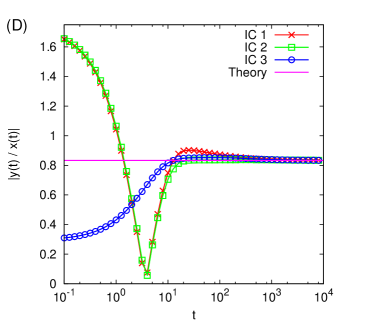
Figure 8: (Color online) Numerical investigation of the behaviour of the reduced model, Eqs. (34), near the coexistence fixed point, $P_{0}$, for $p=\frac{7}{10}$. Panels (A), (B) and (C) show $\widetilde{X}(t)$, $Y(t)$ and $Z(t)$ respectively for three different generic initial conditions. To make the agreement with theory clear, the data have been compensated by the $t$-scalings predicted by Eqs. (39)-(41) with $b(p)$ given by Eq. (38). Panel (D) shows that the ratio $Y(t)/\widetilde{X}(t)$ asymptotically approaches the theoretical prediction $5/6$ (solid line) from Eq. (42).

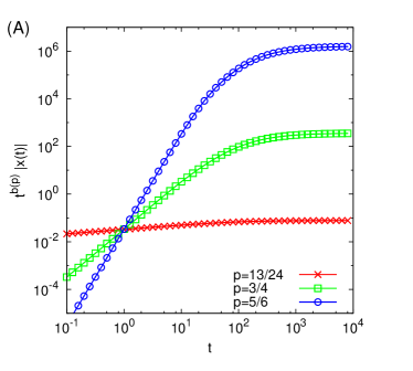
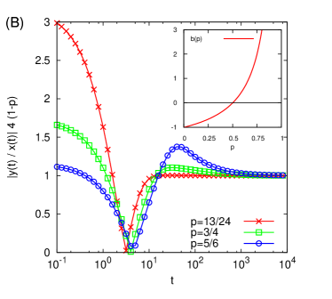
Figure 9: (Color online) Numerical investigation of the behaviour of the reduced model, Eqs. (34), near the coexistence fixed point, $P_{0}$, for a range of values of $p$ for which the fixed point is attractive. Panel (A) shows $\widetilde{X}(t)$ for $p$ taking the values $\frac{13}{24}$(crosses), $\frac{3}{4}$(squares) and $\frac{5}{6}$(circles). The data have been compensated by the $t$-scaling predicted by Eq. (39) with $b(p)$ given by Eq. (38). Panel (B) shows that the ratios $Y(t)/\widetilde{X}(t)$ are in agreement with Eq. (42) for each value of $p$. The inset graphs the dependence of $b(p)$ on $p$ expressed in Eq. (38).

Replacing $\rho_{-}=1-\rho_{+}$ throughout, it is convenient to rewrite Eqs. (29)–(31) in terms of the three variables $(X(t),Y(t),Z(t))$ defined as

$$X = \rho_{+}$$

$$Y = \mu_{+}\rho_{-}-\mu_{-}\rho_{+}$$ (33)

$$Z = (\mu_{+}\rho_{-}+\mu_{-}\rho_{+})^{-1}.$$

In terms of these variables, we have the system

$$\frac{dX}{dt} =\frac{2(2p-1)}{1-Y^{2}Z^{2}}\,X(1-X)YZ\left(1-Z\left|Y\right|\right)$$ (34a)

$$\frac{dY}{dt} =\frac{1}{2}X(1-X)(1-2X)-(1-p)Y$$ (34b)

$$+\frac{2p-1}{2(1-Y^{2}Z^{2})}\,ZF_{Y}(X,Y,Z)$$

$$\frac{dZ}{dt} =\frac{Z^{2}\left[F_{Z}(X,Y,Z)-X(1-X)\right]}{2(1-Y^{2}Z^{2})},$$ (34c)

where $F_{Y}(X,Y,Z)$ and $F_{Z}(X,Y,Z)$ are complicated multivariate polynomials which are written out at the end of this section [Eqs. (43) and (44)]. The advantage of this system is that it is obvious that it has a new fixed point,

$$P_{0}:(X,Y,Z)=\left(\frac{1}{2},0,0\right),$$

which corresponds to the self-similar solution of the full MF equations, Eqs. (7), found in Sec. IV. We refer to $P_{0}$ as the coexistence fixed point since it describes the situation in which both populations have size one half. Note that the consensus fixed points, $P_{-}$ and $P_{+}$ are both mapped to $Z=\infty$ in these variables. Using the system of Eqs. (34) we can try to probe the stability of the coexistence fixed point. The dynamical system given by Eqs. (34) cannot be linearized about $P_{0}$. Notice, for example, that the lowest power of $Z$ in the third equation is $Z^{2}$ so there is no linearization around $Z=0$. Standard methods of linear stability analysis are therefore not applicable here. Instead, let us shift the $X$ variable, $X=\widetilde{X}+\frac{1}{2}$, and look for a scaling solution near $P_{0}$:

$$\widetilde{X}(t) \sim X_{0}\,t^{-a}$$

$$Y(t) \sim Y_{0}\,t^{-b}$$

$$Z(t) \sim Z_{0}\,t^{-c}.$$

The powers $a$, $b$ and $c$ must be all positive if the coexistence fixed point is to be attractive as $t\to\infty$. Some trial and error is required to identify the leading order terms on the RHS of Eqs. (34) due to the large number of terms. However, this work is greatly simplified when we note that all terms that appear in the functions $F_{Y}$ and $F_{Z}$ [Eqs. (43) and (44)] are subleading in the neighbourhood of the coexistence fixed point. Then, the leading terms on the two sides of Eq. (34c) are

$$-c\,Z_{0}\,t^{-c-1}\sim-\frac{1}{8}\,Z_{0}^{2}\,t^{-2c},$$

so that

$$c=1\hskip 7.11317pt\mbox{and}\hskip 7.11317ptZ_{0}=8.$$ (35)

With $c=1$, the leading terms on the two sides of Eq. (34a) are

$$-a\,X_{0}\,t^{-a-1}\sim\frac{1}{2}\,(2\,p-1)\,Y_{0}\,Z_{0}\,t^{-b-c}=4\,(2\,p-1)\,Y_{0}\,t^{-b-1},$$

which leads us to conclude that

$$a=b\hskip 7.11317pt\mbox{and}\hskip 7.11317pt\frac{X_{0}}{Y_{0}}=-\frac{4\,(2\,p-1)}{b}.$$ (36)

Finally, with $c=1$ and $a=b$, the leading terms in Eq. (34b) are

$$-b\,Y_{0}\,t^{-b-1}\sim\left(\frac{-X_{0}}{4}+(p-1)\,Y_{0}\right)t^{-b}.$$

This is impossible unless the coefficient of $t^{-b}$ vanishes on the RHS of Eq. (34b) (there is a subleading term of order $t^{-b-1}$ which could then balance the LHS). Therefore we must have

$$\frac{X_{0}}{Y_{0}}=4\,(p-1).$$ (37)

Combining Eqs. (36) and (37) we find

$$b=-\frac{2\,p-1}{p-1}.$$ (38)

Thus all three exponents are determined along with the amplitude $Z_{0}$. The amplitudes $X_{0}$ and $Y_{0}$ are arbitrary but their ratio is fixed and given by Eq. (37). To summarise, the reduced model predicts the following behaviour near the coexistence fixed point:

$$\widetilde{X}(t) \sim X_{0}\,t^{-b(p)}$$ (39)

$$Y(t) \sim Y_{0}\,t^{-b(p)}$$ (40)

$$Z(t) \sim 8\,t^{-1}$$ (41)

$$\frac{X_{0}}{Y_{0}} = 4\,(p-1),$$ (42)

with $b(p)$ given by Eq. (38). These predictions are validated against numerical solutions of Eqs. (34) in Figs. 8 and 9. We find that $b>0$ for $\frac{1}{2}<p\leq 1$ [see the inset of Fig. 9]. The coexistence fixed point is therefore attractive for values of $p$ in this range and repulsive otherwise. An interesting observation is that the approach of $X$ to the fixed point $X=1/2$ shows damped oscillations for $p\gtrapprox 0.66$, while for $p\lessapprox 0.66$ the approach is monotonic, as we can see in Fig. 10. This transition between the monotonic and the oscillatory regimes is also found in the full MF model [Eqs. (7)] at a value $p_{o}\simeq 0.8$ [see Fig. 10]. In Fig. 10 we also compare the theoretical decay $t^{-b(p)}$ from Eq. (38) (dashed lines) with the one from the MF Eqs. (7) (solid curves), for three different values of $p$. We observe that the agreement improves as $p$ gets larger.

Below we provide for completeness the explicit formulae for the multivariate polynomials appearing on the right hand side of Eqs. (34) defining the reduced model.

$$F_{Y}(X,Y,Z) = -2X^{5}+5X^{4}-4X^{3}-2X^{2}Y+X^{2}-4XY^{2}+2XY+2Y^{3}Z+2Y^{2}+\left(4XY^{2}Z-2Y^{2}Z+2X^{2}YZ\right.$$ (43)

$$\left.-2XYZ-2Y+2X^{5}Z-5X^{4}Z+4X^{3}Z-X^{2}Z\right)\,\left|Y\right|.$$

$$F_{Z}(X,Y,Z) = -X^{2}Y^{2}Z^{2}+2XY^{3}Z^{2}-2XY-Y^{3}Z^{2}+Y+(2p-1)\left[2XY^{3}Z^{2}-Y^{3}Z^{2}+2Y^{2}Z-4X^{3}YZ\right.$$ (44)

$$+6X^{2}YZ-2XYZ+10XY-5Y-X^{4}Z+2X^{3}Z-X^{2}Z+\left(X^{4}Z^{2}+4X^{3}YZ^{2}-2X^{3}Z^{2}-6X^{2}YZ^{2}\right.$$

$$\left.\left.+X^{2}Z^{2}+"XYZ^{2}-12XYZ-2Y^{2}Z^{2}+6YZ\right)\,\left|Y\right|\right].$$

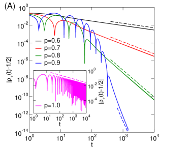
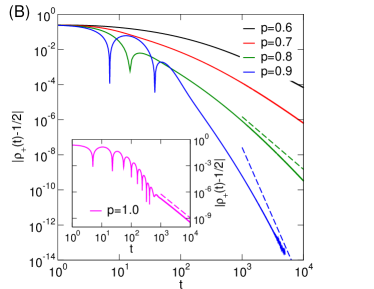
Figure 10: (Color online) Convergence of $\rho_{+}$ to the coexistence state $\rho_{+}=1/2$ for $p>1/2$. (A) Reduced model, Eqs. (29)–(31). The final approach to coexistence is a power law with an exponent given approximately by the theoretical expression $b(p)=(2p-1)/(p-1)$ (dashed lines). Inset: the decay for $p=1.0$ seems to be oscillatory for all times, with an amplitud that decays as $t^{-0.5}$ (dashed line). (B) Full MF equations (7). The approach to coexistence is approximately power law. Dashed lines indicate theoretical exponents $b(p)$. Inset: the $p=1.0$ case is special, where the decay seems to be a pure power law with exponent close to $2.73$ (dashed line).

VI Conclusions

To conclude, we have studied a variant of the voter model in which each agent is endowed with a fitness parameter, $k$, in addition to its opinion variable. Agents interact by pairs, and a single parameter $p$ determines the probability that the agent with the higher $k$–value wins. When an agent wins an interaction, its $k$–value is increased by $1$, and the looser agent changes opinion. The distribution of $k$–values in the population therefore co-evolves with the opinion dynamics. The rates of opinion change therefore depend on the past history of the agents. Our model has aspects in common with several models which have been studied in the literature, particularly the competitive population dynamics studied in Ben-Naim et al. (2006), the Partisan Voter Model Masuda et al. (2010) and the non-Markovian voter model studied in Stark et al. (2008a). Through a combination of numerical simulations and analysis we showed that there is a coexistence state in which both populations have a size similar to $N/2$, and their mean $k$-value increases linearly in time. This coexistence state is attractive on average when $p>1/2$ and repulsive on average when $p<1/2$. As a consequence, the consensus time is increased relative to the standard voter model when $p>1/2$, whereas the system is driven to fast consensus when $p<1/2$. The dynamics in the $p>1/2$ case exhibits interesting properties, including a monotonic approach to the coexistence state, as well as damped oscillations that decay as a power law in time with a non-universal exponent. A quantitative explanation of these stability properties was provided in the context of a reduced 3–D dynamical system based on the full rate equations of the model. One of the outstanding mysteries at this point is that there is little real indication in any of our analysis of why the model with $p=1$ has a larger scaling exponent $\beta\simeq 1.45$ for the consensus time, compared to the exponent $\beta\simeq 1.0$ for $1/2<p<1$ (see Sec. III). This is a topic for future investigation. Another obvious avenue for further investigation would be to study the spatial coarsening properties of the model on regular lattices, since we already know that for $p=1/2$ the coarsening dynamics is equivalent to those in the regular voter model.

References

- Castellano et al. (2009) C. Castellano, S. Fortunato, and V. Loreto, Reviews of Modern Physics 81, 591 (2009).
- Macy and Willer (2002) M. W. Macy and R. Willer, Annual Review of Sociology 28, 143 (2002).
- Ciulla et al. (2012) F. Ciulla, D. Mocanu, A. Baronchelli, B. Gonçalves, N. Perra, and A. Vespignani, EPJ Data Science 1, 1 (2012).
- Preis et al. (2010) T. Preis, D. Reith, and H. E. Stanley, Philosophical Transactions of the Royal Society A: Mathematical, Physical and Engineering Sciences 368, 5707 (2010).
- Conte et al. (2012) R. Conte, N. Gilbert, G. Bonelli, C. Cioffi-Revilla, G. Deffuant, J. Kertesz, V. Loreto, S. Moat, J.-P. Nadal, A. Sanchez, A. Nowak, A. Flache, M. S. Miguel, and D. Helbing, The European Physical Journal Special Topics 214, 325 (2012).
- Krapivsky et al. (2010) P. Krapivsky, S. Redner, and E. Ben-Naim, A Kinetic View of Statistical Physics (Cambridge University Press, Cambridge, 2010).
- Flache and Macy (2011) A. Flache and M. W. Macy, Journal of Conflict Resolution 55, 970 (2011).
- Clifford and Sudbury (1973) P. Clifford and A. Sudbury, Biometrika 60, 581 (1973).
- Holley and M. (1975) R. Holley and L. T. M., Ann. Probab. 4, 195 (1975).
- Liggett (2004) T. M. Liggett, Interacting Particle Systems (Springer, Berlin ; New York, 2004).
- Krapivsky (1992) P. L. Krapivsky, Physical Review A 45, 1067 (1992).
- Vazquez et al. (2003) F. Vazquez, P. L. Krapivsky, and S. Redner, J. Phys. A 36, L61 (2003).
- Vazquez and Redner (2004) F. Vazquez and S. Redner, J. Phys. A 37, 8479 (2004).
- Castelló et al. (2006) X. Castelló, V. M. Eguíluz, and M. San Miguel, New Journal of Physics 8, 308 (2006).
- Antal et al. (2006) T. Antal, S. Redner, and V. Sood, Phys. Rev. Lett. 96, 188104 (2006).
- Medeiros et al. (2006) N. G. F. Medeiros, A. T. C. Silva, and F. G. B. Moreira, Phys. Rev. E 73, 046120 (2006).
- Dall’Asta and Castellano (2007) L. Dall’Asta and C. Castellano, Europhys. Lett. 77, 60005 (2007).
- Dornic et al. (2001) I. Dornic, H. H. Chaté, J. Chave, and H. Hinrichsen, Phys. Rev. Lett. 87, 045701 (2001).
- Al Hammal et al. (2005) O. Al Hammal, H. Chaté, I. Dornic, and M. A. Muñoz, Phys. Rev. Lett. 94, 230601 (2005).
- Vazquez and López (2008) F. Vazquez and C. López, Phys. Rev. E 78, 061127 (2008).
- Mobilia (2003) M. Mobilia, Physical Review Letters 91, 028701 (2003).
- Masuda et al. (2010) N. Masuda, N. Gibert, and S. Redner, Physical Review E 82, 010103 (2010).
- Stark et al. (2008a) H.-U. Stark, C. J. Tessone, and F. Schweitzer, Physical Review Letters 101, 018701 (2008a).
- Stark et al. (2008b) H.-U. Stark, C. J. Tessone, and F. Schweitzer, Advances in Complex Systems 11, 551 (2008b).
- Sood and Redner (2005) V. Sood and S. Redner, Physical Review Letters 94, 178701 (2005).
- Suchecki et al. (2005) K. Suchecki, V. M. Eguíluz, and M. San Miguel, Phys. Rev. E 72, 036132 (2005).
- Vazquez and Eguíluz (2008) F. Vazquez and V. M. Eguíluz, New Journal of Physics 10, 063011 (2008).
- Pérez et al. (2016) T. Pérez, K. Klemm, and V. M. Eguíluz, Scientific Reports 6, 21128 (2016).
- Ben-Naim et al. (2006) E. Ben-Naim, F. Vazquez, and S. Redner, The European Physical Journal B - Condensed Matter and Complex Systems 49, 531 (2006).