Yarkovsky Drift Detections for 247 Near-Earth Asteroids

Abstract

The Yarkovsky effect is a thermal process acting upon the orbits of small celestial bodies, which can cause these orbits to slowly expand or contract with time. The effect is subtle ($\left\langle{da/dt}\right\rangle\sim 10^{-4}$ au/My for a 1 km diameter object) and is thus generally difficult to measure. We analyzed both optical and radar astrometry for 600 near-Earth asteroids (NEAs) for the purpose of detecting and quantifying the Yarkovsky effect. We present 247 NEAs with measured drift rates, which is the largest published set of Yarkovsky detections. This large sample size provides an opportunity to examine the Yarkovsky effect in a statistical manner. In particular, we describe two independent population-based tests that verify the measurement of Yarkovsky orbital drift. First, we provide observational confirmation for the Yarkovsky effect’s theoretical size dependence of 1/$D$, where $D$ is diameter. Second, we find that the observed ratio of negative to positive drift rates in our sample is $2.34$, which, accounting for bias and sampling uncertainty, implies an actual ratio of $2.7^{+0.3}_{-0.7}$. This ratio has a vanishingly small probability of occurring due to chance or statistical noise. The observed ratio of retrograde to prograde rotators is two times lower than the ratio expected from numerical predictions from NEA population studies and traditional assumptions about the sense of rotation of NEAs originating from various main belt escape routes. We also examine the efficiency with which solar energy is converted into orbital energy and find a median efficiency in our sample of 12%. We interpret this efficiency in terms of NEA spin and thermal properties.

1 Introduction

The Yarkovsky effect is a small force that results from the anisotropic thermal emission of small celestial bodies. Over the past decade, there has been increasing awareness that the Yarkovsky effect plays an important role in the evolution of asteroid orbits and the delivery of meteorites to Earth (Bottke et al., 2006). Several authors have published Yarkovsky effect detections for dozens of asteroids: Chesley et al. (2008, 12 detections), Nugent et al. (2012, 54 detections), Farnocchia et al. (2013, 47 detections, of which 21 are deemed reliable).

Here, we provide the largest collection of Yarkovsky detections to date and introduce several improvements to previous studies. Nugent et al. (2012) and Farnocchia et al. (2013) relied on the debiasing of star catalogs proposed by Chesley et al. (2010). Our current model uses the more up-to-date and accurate debiasing algorithm of Farnocchia et al. (2015). Previous works have traditionally relied on a signal-to-noise (S/N) metric and the quantity and quality of the observational data to distinguish between detections and nondetections (Chesley et al., 2008; Farnocchia et al., 2013), or by augmenting these criteria with an explicit sensitivity metric (Nugent et al., 2012). Here, we further refine the detection criterion with a precise formulation based on an analysis of variance (Greenberg et al., 2017). Some of the previous formulations (e.g., Nugent et al., 2012) included a finite increment in semi-major axis at each time step irrespective of the asteroid’s distance from the Sun. Here, we use a 1/$r^{2}$ dependence of the solar flux. The Nugent et al. (2012) results were based on astrometry obtained as of January 31, 2012. The current work benefits from more than 7 years of additional astrometry, including more than 250 additional ranging observations with the Arecibo and Goldstone radars. Finally, the numbers of known NEAs and numbered NEAs have both more than doubled since the Nugent et al. (2012) study. The number of detections is now sufficiently large that ensemble properties can be refined, such as the ratio of retrograde to prograde rotators, and the physical theory can be tested, such as the dependence of the Yarkovsky drift magnitude as a function of asteroid size.

2 Data preparation

Optical astrometry was automatically downloaded from the Minor Planet Center (MPC) on Nov 11, 2019 (Minor Planet Center, 2019). Astrometry taken from nonstationary (generally, space-based) observatories was discarded. Radar astrometry was downloaded from the JPL Radar Astrometry Database (JPL Solar System Dynamics, 2019a) and was discarded from MPC records to avoid duplication. In a few instances, previously unpublished radar data obtained by the authors were also used.

2.1 Weighting and debiasing

Optical astrometry was weighted following the methods described by Farnocchia et al. (2015). To summarize, this method involved weighting measurements based on the observatory, type of measurement, star catalog, and date. We also used the “batched weighting” scheme described by Farnocchia et al. (2015), wherein measurements taken from the same observatory on the same night were given a smaller weight. Star catalog debiasing was also performed according to the approach of Farnocchia et al. (2015).

Radar astrometry was weighted according to observer-reported uncertainties.

2.2 Outlier rejection

Outlier rejection was performed via an iterative fit-drop-add scheme. All available data were used during the initial gravity-only orbital fit. Then, all optical measurements with weighted residuals beyond a fiducial threshold were rejected. This threshold was defined as

$$\frac{(O_{i,RA}-C_{i,RA})^{2}}{\sigma_{i,RA}^{2}}+\frac{(O_{i,DEC}-C_{i,DEC})^{2}}{\sigma_{i,DEC}^{2}}<8,$$ (1)

where $O$ and $C$ stand for observed and computed values, respectively, RA and DEC stand for right ascension and declination, respectively, $\sigma$ represents observational uncertainty, and the index $i$ represents the $i^{th}$ observation.

As the fit iterated, previously discarded measurements were reevaluated with respect to this threshold, and included in subsequent iterations, as appropriate. Outlier rejection was disabled after three fit-drop-add iterations gave identical results.

Initially, outlier rejection was performed with a gravity-only model. After the Yarkovsky component of the dynamical model was estimated, outlier rejection was performed once more with the additional Yarkovsky component included (Section 4).

3 Orbit determination

Orbit determination was performed using our Integration and Determination of Orbits System (IDOS, see Greenberg et al. (2017)). At its core, this software utilizes the Mission analysis, Operations, and Navigation Toolkit Environment (MONTE), a set of tools developed by the Jet Propulsion Laboratory (JPL) for a variety of space-related science and aeronautical goals (Evans et al., 2018). The MONTE orbital integrator can account for gravitational perturbations from any set of masses – for the analyses performed in this paper, we considered the eight known planets and 24 of the most massive minor planets (Folkner et al., 2014) as gravitational perturbers. During close Earth approaches, the integrator considers a detailed model of the planetary gravitational field. MONTE also accounts for general relativistic effects during orbital integration. Further details concerning the internal operations of IDOS were described by Greenberg et al. (2017).

In gravity-only solutions, we estimated the six parameters (three position and three velocity components) of the state vector simultaneously. In Yarkovsky solutions, we estimated an additional parameter describing the strength of the Yarkovsky drift. We assigned one-standard-deviation uncertainties ($\sigma$) to our Yarkovsky estimates such that a 1-$\sigma$ change to the drift rate results in an increase of one in the sum of squares of weighted residuals, similar to the approach of Nugent et al. (2012). This approach yields values that match the formal uncertainties derived from a covariance matrix, which was the approach of Farnocchia et al. (2013).

4 Yarkovsky force model

We utilized the Yarkovsky force model described by Greenberg et al. (2017), where the magnitude and direction of the thermal acceleration, $\ddot{r}$, are calculated and applied at every integration time step of the dynamical model. The acceleration is calculated as

$$\ddot{\vec{r}}=\zeta\;\frac{3}{8\pi}\;\frac{1}{D\rho}\;\frac{L_{\odot}}{c}\;\frac{X_{\hat{p}}(\phi)\vec{r}(t)}{||\vec{r}(t)||^{3}},$$ (2)

where $\vec{r}(t)$ is the heliocentric radial vector for the object at time $t$, $\hat{p}$ is the unit spin-axis vector, $\phi$ is the phase lag, $L_{\odot}$ is the luminosity of the Sun, $c$ is the speed of light, and $X_{\hat{p}}(\phi)$ is the rotation matrix about $\hat{p}$. $D$ and $\rho$ are the diameter and density of the object, respectively, while $\zeta$ is an efficiency factor. The phase lag $\phi$ describes the longitude on the surface from which photons are reemitted, relative to the sub-Solar longitude. In Equation (2), we assume a perfect absorber, i.e., a Bond albedo of zero.

For the objects analyzed in this work, specific values for $\phi$ and $\hat{p}$ were not known. Therefore, these values were fixed at $90^{\text{$\circ$}}$ and antiparallel to the orbit normal vector, respectively , which maximizes the magnitude of the orbital perturbation. As we discuss in the following paragraphs, these assumptions do not affect the estimated value of the semi-major axis drift.

With knowledge of the orbit semi-major axis, $a$, and eccentricity, $e$, the orbit-averaged drift in semi-major axis, $\left\langle{da/dt}\right\rangle$, can be determined from this acceleration model with

$$\left\langle{da/dt}\right\rangle=\pm\;\xi\frac{3}{4\pi}\frac{1}{\sqrt{a}}\frac{1}{1-e^{2}}\frac{L_{\odot}}{c\sqrt{GM_{\odot}}}\frac{1}{D\rho},$$ (3)

which is equivalent to Greenberg et al. (2017)’s equation (8) and corrects Nugent et al. (2012)’s equation (1). Here, $\xi$ is the Yarkovsky efficiency, and depends on $\zeta$, spin pole obliquity $\gamma$ (i.e., the angle between the spin pole vector $\hat{p}$ and the orbit normal vector), and phase lag $\phi$. We always take the Yarkovsky efficiency to be positive. Any incorrect assumption about Bond albedo, diameter, obliquity, and phase lag is absorbed in this efficiency factor such that the $\left\langle{da/dt}\right\rangle$ value, which is dictated by the astrometry, is not affected by these assumptions (Section 14.3).

With numerical values, we find

$$\left\langle{da/dt}\right\rangle=\pm 14.4\left(\frac{\xi}{0.1}\right)\left(\frac{1\text{ au}}{a}\right)^{\frac{1}{2}}\left(\frac{1}{1-e^{2}}\right)\;\times$$ (4)

$$\left(\frac{1\text{ km}}{D}\right)\left(\frac{1000\text{ kg}\text{ m}^{-3}}{\rho}\right)\times\frac{10^{-4}\text{ au}}{\text{My}}.$$

5 Candidate selection

5.1 Initial selection

We considered four sets of Yarkovsky detection candidates. Two sets of candidates, the Nugent12 set and the Farnocchia13 set, represent Yarkovsky detections reported by Nugent et al. (2012) and Farnocchia et al. (2013), respectively. For these objects, we performed our analysis in two ways – first, by using the same observational data as those used by the authors, and second, by using all currently available data (Section 5.2). The Nugent12 set features 54 objects, while the Farnocchia13 set contains 47 objects.

The third set contains objects that had not previously been considered by the other two works but that we determined to be Yarkovsky detection candidates. For the most part, these objects had either not yet been discovered, or had small observation intervals prior to 2012 or early 2013. We identified the new candidates as follows. First, we downloaded the list of 21,135 known NEAs from the MPC on November 11, 2019. Second, for each one of the 2915 numbered NEAs, we computed the Yarkovsky sensitivity metric ($s_{Y}$) described by Nugent et al. (2012). This root-mean-square quantity provides an assessment of the relative sensitivity of selected data sets to drifts in semimajor axis . We used the threshold determined by Nugent et al. (2012) of $s_{Y}\geq 2$. We found that 567 NEAs met this condition.

Nugent et al. (2012) rejected Yarkovsky detections for which there were fewer than 100 astrometric measurements, or for which the observation interval was less than 15 years. However, we reviewed the detections that were discarded due to these criteria in 2012 and found that 90% of them are reliable, i.e., their $\left\langle{da/dt}\right\rangle$ values are consistent with values presented in this work, even after the addition of post-2012 data. In this work, we flag objects that Nugent et al. (2012) would have discarded because of data span or quantity, but we do not discard the detections.

5.2 Selection refinement

After candidate selection, we performed a six-parameter fit to the astrometry using a gravity-only model, followed by a seven-parameter fit which included a Yarkovsky force model. We then performed an analysis of variance (Mandel, 1964) to determine whether the data warrant the use of the Yarkovsky model.

Specifically, we calculated the test statistic

$$F=\frac{\kappa_{\delta}}{\kappa_{Y}}$$ (5)

where

$$\kappa_{\delta}=\frac{\sum_{i=0}^{N}(\frac{O_{i}-C_{0,i}}{\sigma_{i}})^{2}-\sum_{i=0}^{N}(\frac{O_{i}-C_{Y,i}}{\sigma_{i}})^{2}}{m_{Y}-m_{0}}$$ (6)

and

$$\kappa_{Y}=\frac{\sum_{i=0}^{N}(\frac{O_{i}-C_{Y,i}}{\sigma_{i}})^{2}}{N-m_{Y}}.$$ (7)

Here, $C_{0,i}$ is the $i^{th}$ computed value assuming gravity only, $C_{Y,i}$ is the $i^{th}$ computed value assuming our best-fit Yarkovsky model, $O_{i}$ is the $i^{th}$ measurement and $\sigma_{i}$ is the associated uncertainty, $N$ is the number of measurements, and $m_{Y}$, $m_{0}$ are the number of free parameters in the Yarkovsky model ($m_{Y}=7$) and gravity-only model ($m_{0}=6$), respectively.

We then calculated the value

$$p=\int_{x=F}^{x=\infty}f(m_{Y}-m_{0},N-m_{Y},x)dx,$$ (8)

where $f(m_{Y}-m_{0},N-m_{Y},x)$ is the F-distribution probability density function with $m_{Y}-m_{0}$ and $N-m_{Y}$ degrees of freedom. The $p$-value serves as a metric for testing the null hypothesis — namely, that the additional degree of freedom introduced by the Yarkovsky force model is superfluous.

Our initial selection refinement step consisted of discarding those objects for which $p>0.05$, which approximately corresponds to a two-standard-deviation detection threshold. This step rejected 283 objects, leaving 317 objects for further consideration.

We also implemented a robustness test where we eliminated the 10 earliest observations from the optical astrometry of each remaining object. For these objects, we refit the Yarkovsky model with the early observations removed, and rejected any object that no longer met the $p\leq 0.05$ criterion. Objects were also rejected when $p$ was $\leq 0.05$, but the error bars of the Yarkovsky rates with and without the early observations did not overlap. This step rejected 60 objects, leaving 257 objects for further analysis.

Finally, because pre-CCD astrometry can lead to spurious detections (Section 13.7) even with proper weights, we reanalyzed 24 Yarkovsky candidates for which pre-1965 astrometry exists. Specifically, we discarded the pre-1965 astrometry, fit for $\left\langle{da/dt}\right\rangle$ values with the shortened observation intervals, and recomputed $p$-values. Objects that no longer met the $p\leq 0.05$ criterion were flagged. Eight objects failed this test and their Yarkovsky rates require additional verification.

6 Comparison with previous works

Approximately 25% of the objects reported in this work had been previously reported as Yarkovsky detections (Section 5). It is useful to compare our Yarkovsky determinations to these previous works, for two reasons. First, because our results were determined independently of the previous works, a comparison serves as a check on both sets of results. Second, new astrometry has been reported for many of these objects. Therefore, we can study how the results and uncertainties changed in light of new data.

We performed two comparisons with the previous works. In each case, we compared both our absolute Yarkovsky measurements and their associated uncertainties to those of the original works. We first created data sets that roughly matched the observational intervals reported by previous authors, to the nearest calendar year. In doing so, we expect there to be good agreement between our Yarkovsky detections and those of the original works. We do anticipate slight differences introduced by our use of improved debiasing and weighting algorithms (Section 2.1) and by our use of observation sets that are not identical to those used in the original works (e.g., observations at beginning or end of intervals matched to the nearest calendar year, precovery observations, or observations that were remeasured). For our second comparison, we included all available data for all objects. In this case, we expect an overall lower level of agreement because of our use of additional astrometry, which sometimes represent a significant fraction of the available astrometry.

Because we are interested in whether our results match those previously published, it is useful to quantify what we mean by a “match”. We used a metric inspired by mean-comparison tests. Namely, for each object $i$ in the dataset, we calculated

$$z_{i}=\frac{|Y_{t,i}-Y_{p,i}|}{\sqrt{\sigma_{t,i}^{2}+\sigma_{p,i}^{2}}},$$ (9)

where $Y_{t,i},Y_{p,i}$ are this work’s estimated drift rate for object $i$ and the previous work’s estimated drift rate for object $i$, respectively, and $\sigma_{t,i},\sigma_{p,i}$ are this work’s uncertainty for object $i$ and the previous work’s uncertainty for object $i$, respectively. The quantity $z$ therefore represents a significance score. By choosing a threshold value for $z$, we can signal our confidence that our measurement is consistent with that of the original work. We chose a significance threshold of $2.0$, i.e., detection $i$ was considered a match if

$$z_{i}<2.0.$$ (10)

In other words, we concluded that the two measurements matched if we could not reject the hypothesis that the two measurements were drawn from the same distribution at the 95% confidence level.

7 Yarkovsky drift rates

We measured semi-major axis drift rates and calculated Yarkovsky efficiency values for 247 NEAs, shown in Table 1 and ordered by object number. We present drift rates derived from optical measurements, as well as optical plus radar astrometry. A machine-readable file containing the data in this table can be found at http://escholarship.org/uc/item/0pj991hd.

Table 1: Yarkovsky drift measurements for 247 Near-Earth Asteroids. The semi-major axis, $a$, is in au. $e$ is orbital eccentricity. Asteroid diameter $D$ is in km. . Diameters inferred from $H$ magnitude via Equation (13) are flagged with a * . $N_{o}$, $N_{r}$ are the number of optical measurements and radar measurements , respectively. $\left\langle{da/dt}\right\rangle$, $\sigma$, the semi-major axis drift and associated uncertainty, are in $\times 10^{-4}\text{ au/My}$. For objects with radar astrometry ($N_{r}>0$), we also report $\left\langle{da/dt}\right\rangle_{r}$ and $\sigma_{r}$, which incorporate those radar measurements. $p$ and $p_{r}$ are the p-values used in distinguishing between a gravity-only dynamical model and a Yarkovsky dynamical model using optical data only and optical plus radar data, respectively. $s_{Y}$ is the Yarkovsky sensitivity parameter of Nugent et al. (2012). $\xi$ indicates the Yarkovsky efficiency, which was computed with a bulk density that was inferred from the spectral type, if available (Section 10). Yarkovsky detections predicted to be weaker because of the time span or quantity of astrometry (Section 5.1) are flagged with ^†, whereas objects with anomalously high $\xi$ values ($\xi>0.5$) are flagged with ^§. 1Numerical values in this table have been updated.

Name	$a$	$e$	$D$	$N_{o}$	$N_{r}$	$\left\langle{da/dt}\right\rangle$	$\sigma$	$p$	$\left\langle{da/dt}\right\rangle_{r}$	$\sigma_{r}$	$p_{r}$	$s_{Y}$	$\xi$	Arc
(1566) Icarus	1.08	0.83	1.00	2372	16	-4.47	0.4	1e-16	-4.84	0.4	1e-16	37.1	0.03	$1949-2019$
(1620) Geographos	1.25	0.34	2.56	8890	7	-0.68	0.5	3e-03	-1.02	0.5	2e-06	18.7	0.05	$1951-2019$
(1685) Toro	1.37	0.44	3.40	5050	9	-1.52	0.4	1e-16	-1.57	0.4	1e-16	33.0	0.10	$1948-2019$
(1864) Daedalus§	1.46	0.61	3.70	4368	1	-11.29	5.9	6e-05	-11.67	5.8	3e-05	3.0	0.56	$1971-2019$
(1865) Cerberus	1.08	0.47	1.20	3396	0	-3.75	1.8	3e-06	$-$	$-$	$-$	11.5	0.07	$1971-2019$
(1866) SisyphusB	1.89	0.54	8.48	7796	1	-2.26	2.5	2e-02	-2.26	2.5	2e-02	4.3	0.35	$1955-2019$
(1916) Boreas	2.27	0.45	3.50	2892	0	-4.86	2.4	7e-06	$-$	$-$	$-$	7.7	0.39	$1953-2019$
(2062) Aten	0.97	0.18	1.10	1922	7	-6.06	0.9	1e-16	-5.34	0.7	1e-16	24.1	0.10	$1955-2019$
(2063) Bacchus	1.08	0.35	1.02	1292	12	-6.97	2.1	2e-09	-6.22	1.9	1e-08	17.3	0.14	$1977-2016$
(2100) Ra-Shalom	0.83	0.44	2.30	3724	9	-3.27	0.9	3e-16	-2.04	0.6	9e-13	24.8	0.12	$1975-2019$
(2101) Adonis	1.87	0.76	0.60	238	5	-25.43	10.7	1e-03	-17.51	9.3	1e-02	6.5	0.10	$1936-2018$
(2201) Oljato	2.17	0.71	1.80	1950	5	16.28	8.5	1e-04	15.11	7.2	3e-05	2.8	0.47	$1931-2019$
(2202) Pele§	2.29	0.51	∗1.35	500	0	25.07	14.3	3e-04	$-$	$-$	$-$	3.5	0.65	$1972-2018$
(2340) Hathor	0.84	0.45	0.30	902	7	-17.39	0.7	1e-16	-17.61	0.6	1e-16	40.0	0.09	$1976-2019$
(3103) Eger	1.40	0.35	1.50	6534	4	-0.76	2.3	5e-01	-2.83	2.2	4e-03	5.2	0.08	$1982-2019$
(3200) Phaethon	1.27	0.89	6.25	10590	8	-9.01	2.8	8e-13	-9.57	2.1	1e-16	4.6	0.23	$1983-2019$
(3361) Orpheus	1.21	0.32	0.30	1692	0	7.74	1.2	1e-16	$-$	$-$	$-$	22.3	0.04	$1982-2018$
(3362) Khufu	0.99	0.47	0.70	518	0	-17.87	11.8	1e-02	$-$	$-$	$-$	2.9	0.17	$1984-2004$
(3551) Verenia	2.09	0.49	0.90	928	0	-13.11	9.4	2e-02	$-$	$-$	$-$	3.8	0.22	$1983-2019$
(3753) Cruithne	1.00	0.51	2.07	1500	0	-5.14	3.4	1e-03	$-$	$-$	$-$	7.7	0.13	$1973-2019$
(3908) Nyx	1.93	0.46	1.00	3408	16	6.59	2.6	4e-07	7.10	1.6	1e-16	6.3	0.10	$1980-2019$
(4034) Vishnu	1.06	0.44	0.42	960	1	-38.61	9.2	2e-16	-33.04	7.9	4e-16	4.9	0.20	$1986-2015$
(4179) Toutatis	2.54	0.63	5.40	12070	51	-9.52	4.0	4e-10	-2.15	0.3	1e-16	2.0	0.19	$1934-2019$
(4197) Morpheus	2.30	0.77	1.80	1584	6	12.81	8.0	3e-03	13.35	8.0	2e-03	3.2	0.35	$1954-2019$
(4581) Asclepius	1.02	0.36	∗0.26	660	4	-29.91	11.6	8e-09	-20.37	5.4	1e-16	3.2	0.08	$1989-2019$
(4660) Nereus	1.49	0.36	0.33	1338	32	4.26	5.0	8e-02	7.68	3.4	3e-06	7.3	0.05	$1981-2019$
(4688) 1980 WF	2.24	0.51	0.60	416	0	-7.00	5.5	5e-02	$-$	$-$	$-$	9.6	0.06	$1980-2011$
(4769) Castalia	1.06	0.48	1.40	574	15	-5.10	3.0	8e-03	-6.14	2.8	8e-04	10.5	0.12	$1989-2016$
(5011) Ptah	1.64	0.50	∗1.86	1198	0	-14.72	6.4	5e-05	$-$	$-$	$-$	6.3	0.45	$1960-2018$
(5131) 1990 BG§	1.49	0.57	T3.44	3024	0	-16.21	6.5	8e-07	$-$	$-$	$-$	2.0	0.87	$1978-2019$
(5189) 1990 UQ	1.55	0.48	∗0.98	1874	1	-12.22	9.4	2e-03	-12.25	9.4	2e-03	2.3	0.20	$1990-2019$
(5693) 1993 EA	1.27	0.59	∗1.70	3242	0	-6.35	4.3	4e-03	$-$	$-$	$-$	3.4	0.14	$1984-2019$
(5869) Tanith§	1.81	0.32	∗1.29	1176	0	-19.22	14.5	8e-03	$-$	$-$	$-$	2.1	0.51	$1977-2019$
(6239) Minos	1.15	0.41	∗0.71	1762	3	6.79	3.7	3e-04	7.98	3.5	1e-05	7.0	0.09	$1983-2015$
(6456) Golombek§	2.19	0.41	∗2.35	2340	0	-14.08	4.9	6e-11	$-$	$-$	$-$	4.7	0.70	$1979-2019$
(6489) Golevka	2.49	0.61	0.53	1934	20	-13.44	12.1	6e-02	-5.17	0.7	1e-16	1.8	0.05	$1991-2015$
(7336) Saunders	2.31	0.48	T0.52	1786	0	12.44	3.3	7e-15	$-$	$-$	$-$	6.8	0.18	$1982-2018$
(7341) 1991 VK	1.84	0.51	0.98	3040	13	-1.21	3.3	4e-01	-2.57	0.8	2e-12	4.0	0.06	$1981-2018$
(7482) 1994 PC1	1.35	0.33	1.05	1350	1	12.75	8.4	5e-03	13.12	8.4	3e-03	3.4	0.27	$1974-2019$
(7822) 1991 CS	1.12	0.16	1.60	2272	4	8.03	5.6	4e-03	6.57	5.5	2e-02	3.7	0.20	$1991-2016$
(7888) 1993 UCB§	2.44	0.66	2.30	2330	5	-37.71	26.6	5e-03	-37.79	26.5	5e-03	0.5	1.30	$1989-2019$
(7889) 1994 LX	1.26	0.35	1.68	3596	4	-3.92	5.3	1e-01	-6.15	5.2	1e-02	2.3	0.14	$1977-2019$
(8176) 1991 WA	1.57	0.64	T1.48	1304	0	8.60	7.1	5e-02	$-$	$-$	$-$	2.8	0.16	$1991-2019$
(9162) Kwiila	1.50	0.60	1.13	1012	0	-7.06	7.2	5e-02	$-$	$-$	$-$	5.6	0.11	$1987-2019$
(9856) 1991 EE	2.24	0.63	1.00	1536	4	11.84	10.2	5e-03	11.46	10.1	6e-03	2.2	0.18	$1991-2019$
(10302) 1989 ML	1.27	0.14	T0.49	1026	0	19.49	3.7	1e-16	$-$	$-$	$-$	4.4	0.14	$1989-2019$
(10563) Izhdubar	1.01	0.27	T1.55	1092	0	17.09	7.7	4e-04	$-$	$-$	$-$	3.4	0.42	$1991-2019$
(11398) 1998 YP11	1.72	0.39	1.32	5716	0	-5.17	3.6	8e-04	$-$	$-$	$-$	3.0	0.13	$1983-2019$
(11405) 1999 CV3§	1.46	0.39	3.62	4692	0	7.54	5.3	4e-03	$-$	$-$	$-$	2.6	0.66	$1978-2019$
(11500) Tomaiyowit	1.08	0.36	0.74	2010	1	-5.18	2.3	4e-06	-5.45	2.3	5e-07	8.0	0.07	$1989-2019$
(11885) Summanus	1.70	0.47	1.30	542	0	-17.82	10.5	2e-05	$-$	$-$	$-$	3.7	0.40	$1990-2019$
(14402) 1991 DB	1.71	0.40	0.60	1214	0	-6.65	3.1	2e-05	$-$	$-$	$-$	9.3	0.04	$1991-2019$
(15745) Yuliya	1.72	0.26	T1.04	2144	0	-6.00	4.8	1e-02	$-$	$-$	$-$	5.0	0.14	$1982-2019$
(17511) 1992 QN	1.19	0.36	T1.23	2526	1	3.36	3.4	3e-02	3.36	3.4	3e-02	4.7	0.05	$1992-2019$
(18736) 1998 NU§	2.35	0.49	T2.46	3124	0	-15.42	8.3	8e-06	$-$	$-$	$-$	4.2	0.76	$1954-2019$
(31221) 1998 BP26	1.72	0.26	∗1.29	1912	0	-17.06	6.1	8e-09	$-$	$-$	$-$	2.5	0.46	$1998-2019$
(33342) 1998 WT24	0.72	0.42	0.43	3528	16	-10.03	8.3	6e-03	-16.02	2.4	1e-16	2.2	0.08	$1998-2019$
(37655) Illapa	1.48	0.75	∗0.93	1088	2	-11.67	3.6	3e-15	-10.87	3.4	8e-15	9.0	0.09	$1994-2019$
(41429) 2000 GE2	1.59	0.56	0.20	670	0	-31.29	14.9	8e-04	$-$	$-$	$-$	2.5	0.10	$1998-2018$
(52387) Huitzilopochtli	1.28	0.19	0.89	1086	3	-22.51	16.4	6e-03	-22.18	16.3	6e-03	3.3	0.37	$1993-2019$
(54509) YORP†	1.00	0.23	∗0.10	1084	5	-19.97	47.6	3e-01	-33.85	13.3	3e-09	0.7	0.06	$2000-2005$
(65679) 1989 UQ	0.92	0.26	0.92	1382	0	-19.16	4.9	2e-14	$-$	$-$	$-$	5.9	0.26	$1954-2017$
(65690) 1991 DG	1.43	0.36	∗0.56	518	0	-32.45	13.1	3e-05	$-$	$-$	$-$	3.7	0.32	$1991-2018$
(65706) 1992 NA	2.40	0.56	T2.92	1066	0	11.29	10.0	3e-02	$-$	$-$	$-$	2.5	0.33	$1992-2019$
(65733) 1993 PC	1.15	0.47	∗0.78	1394	0	-6.71	4.9	5e-03	$-$	$-$	$-$	4.4	0.07	$1992-2019$
(66146) 1998 TU3	0.79	0.48	2.86	2270	1	-1.60	4.5	4e-01	-5.60	3.9	2e-03	4.1	0.19	$1982-2019$
(66391) MoshupB	0.64	0.69	1.32	7770	37	-5.23	2.9	1e-06	-5.73	2.2	2e-12	2.7	0.04	$1998-2019$
(66400) 1999 LT7	0.86	0.57	0.41	602	0	-38.25	5.3	1e-16	$-$	$-$	$-$	5.4	0.17	$1987-2018$
(68950) 2002 QF15	1.06	0.34	1.65	5124	13	-6.18	5.0	6e-03	-4.72	1.1	1e-16	3.0	0.12	$1955-2019$
(85770) 1998 UP1	1.00	0.35	∗0.28	976	0	-16.56	5.6	8e-07	$-$	$-$	$-$	5.2	0.07	$1990-2016$
(85774) 1998 UT18	1.40	0.33	0.94	1338	8	-3.21	3.8	1e-01	-2.39	0.6	4e-11	5.7	0.02	$1989-2019$
(85953) 1999 FK21	0.74	0.70	0.59	2272	0	-11.64	2.1	1e-16	$-$	$-$	$-$	5.6	0.06	$1971-2018$
(85989) 1999 JD6	0.88	0.63	1.46	5412	15	-6.97	3.7	1e-05	-5.98	3.6	2e-04	3.8	0.12	$1990-2019$
(85990) 1999 JV6	1.01	0.31	0.45	2096	15	-11.40	3.9	4e-07	-14.10	1.0	1e-16	4.3	0.17	$1999-2019$
(87684) 2000 SY2	0.86	0.64	∗2.14	1310	0	-14.35	7.1	3e-04	$-$	$-$	$-$	4.5	0.29	$1977-2019$
(88254) 2001 FM129	1.18	0.63	0.80	1400	2	-10.55	5.8	4e-04	-11.10	5.6	1e-04	5.3	0.10	$1978-2019$
(88959) 2001 TZ44§	1.72	0.56	∗1.18	764	0	-29.45	15.1	4e-04	$-$	$-$	$-$	2.1	0.53	$2001-2019$
(96590) 1998 XB	0.91	0.35	0.88	4764	15	-0.05	4.2	1e+00	2.30	1.1	8e-06	2.7	0.03	$1992-2019$
(99907) 1989 VA	0.73	0.59	1.40	1546	0	12.01	2.5	1e-16	$-$	$-$	$-$	9.0	0.22	$1989-2019$
(101955) Bennu	1.13	0.20	0.49	1148	29	-12.17	4.2	4e-13	-19.03	0.1	1e-16	6.7	0.08	$1999-2018$
(136582) 1992 BA	1.34	0.07	∗0.37	460	0	-20.40	5.9	4e-08	$-$	$-$	$-$	5.3	0.15	$1992-2017$
(136617) 1994 CCB	1.64	0.42	∗1.02	1294	27	-10.92	14.2	2e-01	-13.95	13.3	5e-02	2.1	0.26	$1988-2019$
(136793) 1997 AQ18	1.15	0.47	T1.22	740	0	-22.79	5.3	4e-12	$-$	$-$	$-$	3.8	0.21	$1997-2019$
(136818) Selqet	0.94	0.35	∗0.59	1274	0	8.40	3.2	6e-06	$-$	$-$	$-$	8.3	0.07	$1997-2018$
(136993) 1998 ST49B	2.31	0.60	T1.02	1050	7	26.08	10.1	1e-06	27.22	9.9	3e-07	2.4	0.47	$1998-2019$
(137084) 1998 XS16	1.21	0.50	1.23	3110	0	-17.79	7.0	5e-08	$-$	$-$	$-$	2.2	0.31	$1994-2019$
(137125) 1999 CT3§	1.43	0.13	∗0.65	434	0	-56.44	20.9	1e-06	$-$	$-$	$-$	2.2	0.73	$1999-2018$
(137805) 1999 YK5	0.83	0.56	2.24	2188	0	-6.27	5.3	1e-02	$-$	$-$	$-$	3.1	0.11	$1999-2019$
(137924) 2000 BD19	0.88	0.89	0.97	1304	5	-22.10	13.5	3e-04	-26.17	10.4	5e-08	1.7	0.08	$1997-2019$
(138175) 2000 EE104	1.00	0.29	∗0.31	1870	3	-33.84	7.2	1e-16	-34.59	7.1	1e-16	4.3	0.17	$1999-2019$
(138404) 2000 HA24	1.14	0.32	∗0.54	632	0	12.19	2.8	5e-14	$-$	$-$	$-$	13.2	0.11	$1982-2017$
(138852) 2000 WN10	1.00	0.30	∗0.32	1920	0	16.25	3.7	1e-16	$-$	$-$	$-$	5.6	0.08	$2000-2019$
(138911) 2001 AE2	1.35	0.08	T0.51	1134	0	-12.30	5.8	2e-04	$-$	$-$	$-$	5.5	0.13	$1984-2017$
(139622) 2001 QQ142§	1.42	0.31	T0.66	938	0	-31.92	14.4	2e-06	$-$	$-$	$-$	2.5	0.54	$2001-2019$
(141018) 2001 WC47	1.40	0.24	∗0.59	2962	4	-5.41	7.4	7e-02	-7.49	7.0	7e-03	2.0	0.08	$1991-2019$
(141498) 2002 EZ16	0.92	0.57	∗0.74	624	0	-12.01	11.2	3e-02	$-$	$-$	$-$	3.3	0.10	$1995-2019$
(141531) 2002 GB	0.99	0.53	0.30	1396	0	23.50	12.5	1e-03	$-$	$-$	$-$	2.1	0.09	$2002-2019$
(152563) 1992 BF	0.91	0.27	0.27	712	0	-13.99	1.3	1e-16	$-$	$-$	$-$	20.3	0.11	$1953-2018$
(152671) 1998 HL3	1.13	0.37	0.30	632	0	-31.92	9.3	1e-10	$-$	$-$	$-$	3.9	0.15	$1998-2018$
(152742) 1998 XE12	0.88	0.74	0.41	666	0	14.11	10.9	3e-02	$-$	$-$	$-$	2.6	0.04	$1995-2019$
(152754) 1999 GS6	1.19	0.50	0.41	744	0	-11.14	4.3	1e-09	$-$	$-$	$-$	8.5	0.06	$1999-2019$
(153201) 2000 WO107	0.91	0.78	0.51	852	0	-24.37	12.7	9e-04	$-$	$-$	$-$	2.2	0.06	$2000-2018$
(153814) 2001 WN5§	1.71	0.47	0.93	1632	2	34.10	9.7	5e-14	38.78	9.3	1e-16	2.4	0.63	$1996-2019$
(154590) 2003 MA3	1.11	0.40	0.09	224	0	-46.44	10.8	6e-16	$-$	$-$	$-$	5.4	0.06	$1998-2018$
(161999) 1989 RC	2.32	0.51	0.46	206	0	-38.20	21.8	3e-03	$-$	$-$	$-$	2.8	0.34	$1989-2018$
(162004) 1991 VE	0.89	0.66	∗0.81	1870	2	18.36	3.5	1e-16	21.44	2.7	1e-16	4.7	0.16	$1954-2019$
(162080) 1998 DG16	0.90	0.36	0.78	244	0	-18.26	7.1	1e-05	$-$	$-$	$-$	3.1	0.20	$1981-2015$
(162082) 1998 HL1	1.25	0.19	∗0.59	1834	0	-12.44	5.4	1e-06	$-$	$-$	$-$	3.7	0.14	$1998-2019$
(162117) 1998 SD15	0.93	0.34	∗0.56	1048	0	-9.29	1.6	1e-16	$-$	$-$	$-$	14.6	0.08	$1998-2018$
(162142) 1998 VR	0.88	0.32	0.46	818	0	9.05	3.0	4e-07	$-$	$-$	$-$	9.8	0.06	$1998-2016$
(162162) 1999 DB7	1.21	0.19	∗0.37	520	0	18.95	11.3	3e-03	$-$	$-$	$-$	5.2	0.13	$1999-2019$
(162173) Ryugu	1.19	0.19	T0.77	1444	0	-15.99	6.7	2e-07	$-$	$-$	$-$	3.6	0.09	$1986-2016$
(162181) 1999 LF6	1.41	0.28	0.73	2980	2	-12.04	2.9	1e-16	-9.92	2.8	2e-12	5.2	0.14	$1979-2019$
(162361) 2000 AF6	0.88	0.41	∗0.34	778	0	21.89	4.2	1e-16	$-$	$-$	$-$	7.0	0.10	$1991-2019$
(162463) 2000 JH5§	1.15	0.24	1.05	970	0	-28.09	11.6	2e-06	$-$	$-$	$-$	2.2	0.51	$2000-2017$
(162483) 2000 PJ5	0.87	0.37	0.91	860	0	-8.95	7.9	2e-02	$-$	$-$	$-$	3.6	0.11	$2000-2018$
(162567) 2000 RW37	1.25	0.25	0.34	388	0	-16.65	14.2	2e-02	$-$	$-$	$-$	3.8	0.05	$2000-2018$
(162694) 2000 UH11	0.87	0.42	∗0.43	414	0	-30.62	9.3	1e-09	$-$	$-$	$-$	4.7	0.17	$2000-2017$
(162783) 2000 YJ11	1.31	0.23	∗0.26	262	0	-47.51	15.8	9e-09	$-$	$-$	$-$	5.3	0.23	$2000-2018$
(162882) 2001 FD58	1.09	0.58	∗0.65	784	3	-14.50	8.2	8e-04	-13.90	8.1	1e-03	3.6	0.11	$2000-2018$
(163000) 2001 SW169	1.25	0.05	∗0.51	2004	0	-8.26	4.3	8e-05	$-$	$-$	$-$	4.3	0.08	$1997-2019$
(163023) 2001 XU1	0.80	0.55	∗0.49	634	0	34.25	8.9	1e-16	$-$	$-$	$-$	3.0	0.18	$2001-2019$
(163081) 2002 AG29	1.09	0.20	∗0.74	816	0	13.60	7.9	1e-03	$-$	$-$	$-$	5.3	0.17	$1985-2019$
(163348) 2002 NN4†	0.88	0.43	0.73	672	0	13.20	10.1	4e-02	$-$	$-$	$-$	3.4	0.13	$2002-2016$
(164202) 2004 EW†	0.99	0.28	∗0.25	844	0	18.70	13.0	2e-02	$-$	$-$	$-$	2.5	0.07	$2004-2017$
(164207) 2004 GU9	1.00	0.14	0.16	442	0	-31.71	11.5	9e-07	$-$	$-$	$-$	4.2	0.09	$2001-2019$
(175706) 1996 FG3B	1.05	0.35	1.20	3214	7	-13.13	5.6	8e-09	-18.74	4.9	1e-16	3.1	0.19	$1985-2014$
(185851) 2000 DP107B	1.37	0.38	0.86	2838	13	-0.82	2.8	6e-01	5.45	2.3	5e-06	4.3	0.04	$2000-2019$
(190491) 2000 FJ10	1.32	0.23	∗0.23	502	0	-26.02	16.7	2e-02	$-$	$-$	$-$	2.2	0.11	$2000-2017$
(190758) 2001 QH96§	1.75	0.36	∗0.74	470	0	49.52	27.1	2e-04	$-$	$-$	$-$	2.7	0.72	$1994-2017$
(192559) 1998 VO	1.07	0.23	∗0.31	1196	0	-14.46	4.1	1e-16	$-$	$-$	$-$	6.4	0.08	$1998-2018$
(192563) 1998 WZ6	1.45	0.41	T1.23	1470	0	-20.06	7.6	1e-06	$-$	$-$	$-$	2.6	0.33	$1998-2019$
(203471) 2002 AU4	0.86	0.37	∗0.47	700	0	-13.61	7.5	1e-03	$-$	$-$	$-$	6.6	0.09	$1994-2017$
(208023) 1999 AQ10	0.93	0.24	T0.28	876	3	-24.34	6.8	1e-16	-23.37	5.9	1e-16	4.3	0.10	$1999-2018$
(215442) 2002 MQ3	0.91	0.27	1.07	664	0	-20.47	12.0	4e-04	$-$	$-$	$-$	2.2	0.33	$2002-2017$
(216523) 2001 HY7	0.91	0.41	∗0.27	572	0	30.75	6.0	1e-16	$-$	$-$	$-$	6.1	0.11	$2001-2016$
(216985) 2000 QK130	1.18	0.26	∗0.21	488	0	44.61	7.8	1e-16	$-$	$-$	$-$	5.7	0.17	$2000-2018$
(217628) Lugh§	2.55	0.70	1.40	240	0	-97.09	40.0	9e-06	$-$	$-$	$-$	2.2	1.88	$1960-2019$
(230111) 2001 BE10	0.82	0.37	∗0.54	1504	3	-13.76	5.5	1e-07	-12.79	5.3	2e-07	5.1	0.09	$2001-2019$
(230549) 2003 BH	1.46	0.36	0.22	306	0	25.48	15.1	3e-03	$-$	$-$	$-$	2.7	0.10	$2003-2019$
(232691) 2004 AR1	1.58	0.47	∗0.39	614	4	-34.91	14.8	8e-06	-35.22	13.7	1e-06	2.0	0.23	$2004-2019$
(240320) 2003 HS42	1.46	0.12	∗0.34	276	0	31.87	19.6	1e-02	$-$	$-$	$-$	2.7	0.22	$1998-2019$
(242191) 2003 NZ6†	0.79	0.49	0.37	914	3	23.64	8.4	4e-10	24.30	8.3	1e-10	2.7	0.10	$2003-2017$
(243025) 2006 UM216	2.68	0.52	2.12	1258	0	-10.50	12.2	3e-02	$-$	$-$	$-$	3.2	0.45	$1954-2019$
(244670) 2003 KN18	1.75	0.49	∗0.71	824	0	34.67	16.8	5e-07	$-$	$-$	$-$	2.1	0.42	$1989-2019$
(247517) 2002 QY6	0.82	0.70	0.27	710	0	-25.72	12.3	9e-04	$-$	$-$	$-$	3.1	0.05	$2002-2019$
(249886) 2001 RY11§	1.48	0.28	1.20	692	0	31.39	21.7	8e-03	$-$	$-$	$-$	3.0	0.72	$1992-2019$
(252399) 2001 TX44	0.87	0.55	0.29	466	0	-36.80	11.8	4e-08	$-$	$-$	$-$	4.2	0.12	$2001-2019$
(252558) 2001 WT1	1.09	0.40	0.53	466	0	-34.23	14.6	3e-04	$-$	$-$	$-$	2.8	0.27	$2001-2018$
(253062) 2002 TC70	1.37	0.20	∗0.22	416	0	-27.23	9.4	2e-10	$-$	$-$	$-$	4.7	0.12	$2002-2018$
(256004) 2006 UP†	1.59	0.30	∗0.09	328	0	-65.16	19.5	2e-08	$-$	$-$	$-$	2.4	0.11	$2002-2016$
(265482) 2005 EE†	1.13	0.33	∗0.20	768	5	41.08	12.4	2e-16	48.61	11.3	1e-16	2.9	0.16	$2004-2017$
(267940) 2004 EM20	1.11	0.52	∗0.31	520	0	-25.61	10.1	3e-06	$-$	$-$	$-$	4.3	0.10	$2004-2019$
(276033) 2002 AJ129	1.37	0.91	∗0.65	928	5	21.84	14.7	1e-02	26.57	14.6	3e-03	2.1	0.06	$2002-2018$
(276770) 2004 HC†	0.79	0.60	∗0.37	416	0	-38.11	25.3	3e-03	$-$	$-$	$-$	2.1	0.14	$2004-2018$
(297418) 2000 SP43	0.81	0.47	0.41	1612	1	-15.02	3.5	1e-16	-15.03	3.5	1e-16	6.4	0.07	$2000-2019$
(302169) 2001 TD45	0.80	0.78	∗0.37	206	0	-11.92	11.5	4e-02	$-$	$-$	$-$	5.0	0.03	$2001-2019$
(306383) 1993 VD	0.88	0.55	∗0.18	306	1	-22.18	5.0	1e-15	-18.82	4.5	6e-14	8.0	0.04	$1993-2018$
(307070) 2002 AV31	1.31	0.25	0.28	500	0	-21.67	10.9	2e-03	$-$	$-$	$-$	4.7	0.11	$2002-2019$
(310442) 2000 CH59	0.86	0.42	∗0.37	664	0	28.82	6.8	3e-13	$-$	$-$	$-$	4.8	0.14	$2000-2017$
(310842) 2003 AK18†	0.88	0.38	∗0.41	1014	4	-18.29	5.9	2e-09	-17.90	5.8	1e-09	4.5	0.10	$2003-2017$
(322756) 2001 CK32	0.73	0.38	∗0.56	296	0	-15.03	14.3	4e-02	$-$	$-$	$-$	2.9	0.11	$2001-2017$
(326302) 1998 VN	1.39	0.34	∗0.28	386	0	-38.48	18.9	5e-04	$-$	$-$	$-$	2.0	0.19	$1998-2019$
(326354) 2000 SJ344	1.14	0.17	∗0.10	126	0	-64.77	15.6	1e-16	$-$	$-$	$-$	5.8	0.12	$2000-2018$
(326683) 2002 WP	1.45	0.22	0.52	1602	1	11.98	5.4	3e-06	12.38	5.3	9e-07	4.3	0.13	$2002-2019$
(330659) 2008 GG2†	1.59	0.28	∗0.09	406	0	29.18	9.8	1e-07	$-$	$-$	$-$	5.4	0.05	$2004-2018$
(333889) 1998 SV4	0.82	0.64	0.92	1170	0	7.94	8.5	4e-02	$-$	$-$	$-$	3.2	0.07	$1998-2018$
(334412) 2002 EZ2	1.25	0.05	∗0.32	1012	0	-19.02	7.1	2e-06	$-$	$-$	$-$	4.3	0.12	$2002-2019$
(337084) 1998 SE36	1.34	0.10	∗0.41	704	0	-26.97	13.6	5e-06	$-$	$-$	$-$	2.5	0.22	$1998-2018$
(337248) 2000 RH60	0.83	0.55	0.85	734	0	-17.45	8.1	8e-05	$-$	$-$	$-$	4.3	0.16	$2000-2018$
(337252) 2000 SD8	1.13	0.31	∗0.25	310	0	-32.76	9.2	4e-11	$-$	$-$	$-$	5.7	0.13	$2000-2018$
(338292) 2002 UA31	0.80	0.49	∗0.56	696	0	-18.97	8.0	6e-06	$-$	$-$	$-$	3.3	0.12	$2002-2017$
(339714) 2005 ST1	1.45	0.37	∗0.30	780	0	-7.84	3.9	5e-04	$-$	$-$	$-$	8.8	0.04	$1991-2019$
(344074) 1997 UH9	0.83	0.47	T0.54	684	0	32.34	9.8	7e-09	$-$	$-$	$-$	3.1	0.30	$1997-2019$
(348306) 2005 AY28†	0.87	0.57	∗0.18	448	2	-62.53	21.1	1e-06	-64.77	21.1	7e-07	3.1	0.12	$2005-2018$
(350462) 1998 KG3	1.16	0.12	∗0.14	440	0	-26.68	4.1	1e-16	$-$	$-$	$-$	9.9	0.07	$1998-2018$
(350523) 2000 EA14	1.12	0.20	∗0.21	342	0	24.05	7.3	7e-08	$-$	$-$	$-$	8.5	0.09	$2000-2019$
(351545) 2005 TE15†	1.20	0.34	∗0.41	446	0	-26.73	16.7	9e-03	$-$	$-$	$-$	2.2	0.18	$2005-2017$
(358453) 2007 EH88	1.12	0.44	∗0.39	404	0	-50.08	16.6	6e-08	$-$	$-$	$-$	2.7	0.28	$1994-2019$
(363027) 1998 ST27B	0.82	0.53	0.58	750	7	14.92	8.9	1e-03	14.11	4.1	4e-11	2.6	0.09	$1998-2018$
(363116) 2001 GQ2	1.21	0.50	∗0.34	1150	3	-10.29	8.2	2e-03	-9.80	8.1	3e-03	3.4	0.05	$2001-2017$
(363599) 2004 FG11B†	1.59	0.72	0.15	530	8	-34.66	7.5	1e-16	-38.02	6.7	1e-16	5.2	0.06	$2004-2018$
(364136) 2006 CJ†	0.68	0.75	∗0.32	698	10	-24.97	10.3	3e-07	-38.23	1.8	1e-16	4.0	0.07	$2006-2017$
(369986) 1998 SO	0.73	0.70	∗0.27	438	0	12.29	8.2	2e-03	$-$	$-$	$-$	6.1	0.02	$1998-2018$
(376879) 2001 WW1	1.21	0.12	∗0.13	204	0	-27.37	10.5	7e-06	$-$	$-$	$-$	6.0	0.07	$2001-2017$
(385186) 1994 AW1B	1.11	0.08	0.81	3176	3	4.06	2.8	4e-04	4.08	2.7	2e-04	6.3	0.03	$1986-2017$
(396593) 2001 HC	0.87	0.50	∗0.56	540	0	13.86	5.0	3e-13	$-$	$-$	$-$	8.7	0.09	$2001-2019$
(398188) Agni	0.86	0.27	0.46	628	13	-28.74	10.6	1e-07	-22.41	8.8	5e-07	3.1	0.15	$2001-2018$
(399308) 1993 GD	1.10	0.24	∗0.26	204	0	44.64	9.6	2e-12	$-$	$-$	$-$	5.7	0.19	$1993-2015$
(401885) 2001 RV17†	0.91	0.34	∗0.28	360	0	-19.09	8.8	4e-04	$-$	$-$	$-$	5.4	0.08	$2001-2015$
(410777) 2009 FDB†	1.16	0.49	0.47	998	8	38.18	15.1	1e-07	41.25	14.7	1e-08	1.6	0.27	$2009-2019$
(412976) 1987 WC	1.36	0.23	∗0.39	324	0	32.95	12.3	2e-05	$-$	$-$	$-$	3.4	0.24	$1987-2017$
(413260) 2003 TL4	0.78	0.38	∗0.47	864	10	-20.94	7.2	4e-12	-20.58	4.5	1e-16	3.7	0.12	$2003-2018$
(415711) 1998 WT7	1.15	0.11	0.35	358	0	35.71	18.3	7e-04	$-$	$-$	$-$	3.4	0.22	$1998-2019$
(416151) 2002 RQ25†	1.11	0.31	∗0.26	426	6	16.72	12.9	5e-02	17.88	9.7	3e-03	3.4	0.08	$2002-2016$
(418849) 2008 WM64†	1.01	0.11	∗0.27	432	4	-21.42	12.8	2e-03	-29.33	11.1	7e-06	2.6	0.13	$2008-2019$
(433953) 1997 XR2	1.08	0.20	0.26	802	8	14.81	9.7	9e-03	11.37	7.7	1e-02	3.2	0.05	$1997-2017$
(437841) 1998 HD14	0.96	0.31	∗0.22	386	0	-33.82	9.4	2e-12	$-$	$-$	$-$	6.9	0.11	$1998-2019$
(437844) 1999 MN	0.67	0.67	∗0.19	270	4	37.93	3.9	1e-16	37.42	3.8	1e-16	9.6	0.05	$1999-2015$
(437846) 1999 RJ27§	1.48	0.35	∗0.47	194	0	-60.34	24.4	1e-04	$-$	$-$	$-$	2.8	0.51	$1999-2019$
(438661) 2008 EP6†	1.21	0.29	∗0.47	284	1	-1.43	44.8	9e-01	-30.46	29.3	1e-02	2.2	0.25	$2008-2019$
(441987) 2010 NY65†	1.00	0.37	0.23	1286	15	15.34	17.2	8e-02	-17.95	0.9	1e-16	1.2	0.06	$2010-2019$
(443837) 2000 TJ1	1.16	0.08	0.25	686	0	-9.71	7.1	2e-03	$-$	$-$	$-$	5.7	0.05	$2000-2015$
(446924) 2002 VV17	0.84	0.44	∗0.32	888	0	-16.00	6.9	2e-06	$-$	$-$	$-$	4.3	0.07	$1992-2018$
(450293) 2004 LV3	1.23	0.28	∗0.62	718	5	-20.06	16.9	5e-02	-22.85	16.8	2e-02	2.0	0.25	$2004-2019$
(450300) 2004 QD14†	0.94	0.34	∗0.28	274	0	-59.01	26.2	7e-04	$-$	$-$	$-$	2.0	0.24	$2004-2017$
(452389) 2002 NW16	1.11	0.03	0.85	2218	0	-9.33	5.4	1e-03	$-$	$-$	$-$	2.8	0.14	$2002-2017$
(455146) 1993 FS	2.23	0.42	∗0.43	200	0	38.47	17.9	7e-04	$-$	$-$	$-$	3.4	0.34	$1993-2016$
(455176) 1999 VF22	1.31	0.74	∗0.27	364	3	-37.68	7.0	1e-16	-37.40	6.9	1e-16	7.9	0.09	$1999-2019$
(455184) 2000 ED14	0.83	0.57	∗0.25	322	1	29.29	19.5	7e-03	29.14	19.5	8e-03	2.3	0.08	$2000-2019$
(455415) 2003 GA	1.28	0.19	∗0.20	694	0	33.76	28.8	3e-02	$-$	$-$	$-$	2.1	0.13	$2003-2019$
(455594) 2004 SV55†	1.76	0.66	1.62	498	0	-11.89	9.4	7e-03	$-$	$-$	$-$	3.9	0.25	$2004-2018$
(461353) 1999 LS7	1.01	0.30	∗0.25	252	0	-48.53	22.9	4e-04	$-$	$-$	$-$	2.0	0.19	$1999-2016$
(461852) 2006 GY2B†§	1.86	0.50	∗0.62	596	9	-370.26	169.2	4e-05	-319.58	156.9	2e-04	0.2	3.47	$2006-2016$
(467336) 2002 LT38†	0.85	0.31	∗0.28	606	0	11.66	6.2	2e-03	$-$	$-$	$-$	5.9	0.05	$2002-2016$
(468468) 2004 KH17	0.71	0.50	0.20	424	1	-43.80	5.3	1e-16	-43.81	5.3	1e-16	5.9	0.09	$2004-2019$
(469445) 2002 LT24†	0.72	0.50	0.14	370	0	-29.65	18.6	2e-02	$-$	$-$	$-$	2.3	0.05	$2002-2016$
(469737) 2005 NW44†	0.78	0.48	∗0.30	792	0	15.34	6.6	1e-05	$-$	$-$	$-$	4.5	0.05	$2005-2018$
(474158) 1999 FA	1.08	0.13	T0.22	440	0	-41.23	9.2	1e-16	$-$	$-$	$-$	2.2	0.17	$1978-2016$
(474163) 1999 SO5	1.09	0.07	∗0.23	506	0	-27.84	11.3	2e-04	$-$	$-$	$-$	3.3	0.12	$1999-2017$
(474574) 2004 FG1†	1.75	0.29	∗0.47	772	0	-32.77	18.5	5e-05	$-$	$-$	$-$	2.1	0.32	$2004-2018$
(480808) 1994 XL1	0.67	0.53	∗0.23	346	0	-31.77	3.5	1e-16	$-$	$-$	$-$	16.0	0.08	$1994-2016$
(480883) 2001 YE4	0.68	0.54	∗0.26	686	7	-48.47	2.0	1e-16	-49.84	0.7	1e-16	9.9	0.13	$2001-2017$
(481442) 2006 WO3	0.80	0.45	∗0.17	572	0	-41.73	9.0	1e-16	$-$	$-$	$-$	3.7	0.09	$2001-2016$
(483459) 2002 EM6	1.16	0.14	∗0.32	526	0	18.42	7.7	3e-04	$-$	$-$	$-$	4.8	0.11	$2002-2017$
(483656) 2005 ES70†	0.76	0.39	∗0.06	332	1	-79.85	3.2	1e-16	-79.57	3.1	1e-16	11.1	0.06	$2005-2019$
(488453) 1994 XDB	2.35	0.73	∗0.54	594	8	41.69	28.0	1e-03	35.27	23.2	1e-03	0.8	0.23	$1994-2017$
(488789) 2004 XK50†§	1.45	0.69	1.04	180	0	56.04	37.3	1e-02	$-$	$-$	$-$	2.2	0.63	$2004-2018$
(494658) 2000 UG11B	1.93	0.57	∗0.30	846	4	-34.96	42.7	4e-02	-55.71	42.0	1e-03	0.7	0.26	$2000-2017$
(494710) 2005 MO13	0.86	0.41	∗0.25	454	0	-31.06	7.1	2e-11	$-$	$-$	$-$	5.4	0.10	$2001-2017$
(495829) 1995 LG	1.06	0.79	∗0.65	582	0	10.13	5.3	9e-04	$-$	$-$	$-$	7.5	0.04	$1995-2019$
(497113) 2004 EK1†	1.25	0.25	∗0.13	424	0	-17.04	10.3	2e-03	$-$	$-$	$-$	5.0	0.04	$2004-2018$
(499998) 2011 PT†	1.31	0.22	∗0.06	394	0	-88.44	14.6	1e-16	$-$	$-$	$-$	2.8	0.10	$2011-2017$
(503941) 2003 UV11	1.45	0.76	0.26	1736	14	-1.04	3.9	6e-01	6.39	2.1	4e-10	5.4	0.01	$1996-2017$
(506590) 2005 XB1†	1.13	0.42	0.10	234	0	46.63	9.3	1e-16	$-$	$-$	$-$	7.0	0.07	$2005-2017$
(513126) 1998 QP	1.79	0.58	∗0.20	500	0	-38.42	29.1	1e-02	$-$	$-$	$-$	3.1	0.12	$1998-2018$
(513312) 2007 DM41†	1.18	0.53	∗0.14	420	0	39.66	19.1	6e-05	$-$	$-$	$-$	2.2	0.08	$2007-2017$
(516435) 2004 FJ29†	0.91	0.35	∗0.20	306	0	-15.93	9.2	2e-03	$-$	$-$	$-$	5.2	0.04	$2004-2018$
(523586) 1999 LK1	0.91	0.33	∗0.14	216	0	-9.87	8.7	1e-02	$-$	$-$	$-$	5.3	0.02	$1999-2019$
(523595) 2002 OS4	1.92	0.45	0.66	1414	0	-9.38	9.5	3e-02	$-$	$-$	$-$	2.1	0.12	$2002-2019$
(523605) 2004 RX10	0.92	0.35	∗0.20	392	0	-29.63	7.0	2e-15	$-$	$-$	$-$	6.1	0.08	$2004-2019$
(523934) 1998 FF14	1.25	0.31	∗0.26	246	0	-17.72	7.1	2e-05	$-$	$-$	$-$	9.6	0.08	$1998-2019$
(524522) 2002 VE68	0.72	0.41	∗0.28	1142	10	-34.90	1.8	1e-16	-35.35	0.6	1e-16	13.5	0.12	$2002-2018$
(526798) 2007 AA9†	0.86	0.42	∗0.12	138	0	-68.86	35.9	4e-03	$-$	$-$	$-$	2.1	0.11	$2007-2019$
2004 BG41†	2.51	0.61	∗0.05	174	0	-51.25	30.0	8e-03	$-$	$-$	$-$	-1.0	0.04	$2004-2015$
2004 SC56†	0.77	0.43	0.29	324	0	-42.91	27.8	2e-03	$-$	$-$	$-$	-1.0	0.15	$2004-2010$
2009 BD†	1.06	0.05	∗0.01	366	0	-381.69	99.3	6e-13	$-$	$-$	$-$	-1.0	0.06	$2009-2011$

Table 2: Yarkovsky drift measurements for 8 Near-Earth Asteroids whose rates require additional verifications because solutions that include pre-1965 astrometry, shown here, differ from solutions that exclude pre-1965 astrometry. Columns as in Table 1. 1This is a new table.

Name	$a$	$e$	$D$	$N_{o}$	$N_{r}$	$\left\langle{da/dt}\right\rangle$	$\sigma$	$p$	$\left\langle{da/dt}\right\rangle_{r}$	$\sigma_{r}$	$p_{r}$	$s_{Y}$	$\xi$	Arc
(433) Eros†	1.46	0.22	16.84	16850	5	-0.49	0.2	1e-13	-0.43	0.1	2e-13	66.3	0.15	$1900-2019$
(719) Albert†	2.64	0.55	T2.38	3604	0	-1.83	1.4	3e-04	$-$	$-$	$-$	11.9	0.09	$1911-2019$
(1036) Ganymed†§	2.66	0.53	37.67	12028	1	-4.98	1.3	1e-16	-4.98	1.3	1e-16	6.4	4.14	$1924-2019$
(1862) ApolloB†	1.47	0.56	1.50	3216	17	-0.30	0.9	5e-01	-1.78	0.2	1e-16	28.9	0.04	$1930-2019$
(1915) Quetzalcoatl†	2.54	0.57	0.50	96	1	-42.38	23.0	3e-02	-45.18	22.7	2e-02	4.0	0.41	$1953-2004$
(2061) Anza†	2.26	0.54	2.60	1822	0	3.29	3.8	5e-02	$-$	$-$	$-$	6.2	0.16	$1960-2019$
(4015) Wilson-Harrington†§	2.63	0.63	4.00	1874	0	-7.57	3.1	1e-04	$-$	$-$	$-$	10.3	0.51	$1949-2019$
(29075) 1950 DA†	1.70	0.51	2.00	1180	12	-3.92	1.8	2e-05	-2.61	0.5	1e-16	13.3	0.09	$1950-2019$

8 Comparison with Nugent et al. (2012)

8.1 Using matching observation intervals

We analyzed the 54 Yarkovsky objects described by Nugent et al. (2012) by constructing observation intervals whose calendar years matched those listed in Table 3 of that work. We compared (Section 6) our results with their findings (Figure 1). We agreed with all $\left\langle{da/dt}\right\rangle$ values save one, (4179) Toutatis, for which we found a $z$-score of 2.68. We examine this object in more detail in Section 13.5.

However, we also found that 16 objects that Nugent et al. (2012) identified as detections did not pass our detection threshold (Section 5.2). Much of this discrepancy is explained by this work’s higher threshold for detection — a $p$-value of 0.05 approximately corresponds to an S/N of 2, while Nugent et al. (2012) considered possible detections for objects with S/N $>$ 1. Indeed, all but two of the 16 objects exhibit 1 $<$ S/N $<$ 2 in Nugent et al. (2012)’s table.

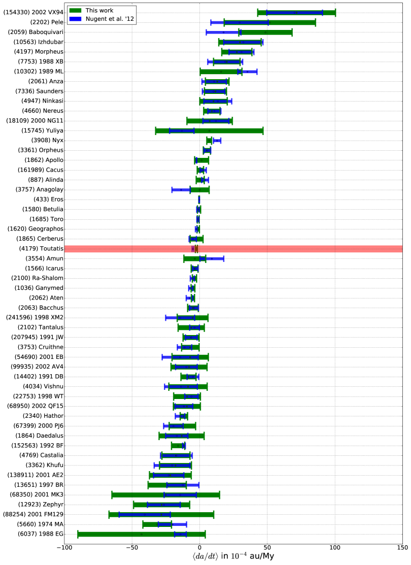
Figure 1: A comparison of our Yarkovsky detections (green) and those determined by Nugent et al. (2012) (blue), when we used only matching data. Measurements that disagreed (i.e., $z_{i}>2$, Section 6) are highlighted in red. Objects are ranked from most positive to most negative Yarkovsky drift rate.

8.2 Using all available data

When using all available data (including data that were not available for use by Nugent et al. (2012)), we found good agreement (Figure 2), except for three objects — (4179) Toutatis, and (5660) 1974 MA — for which our drift rates do not match those of Nugent et al. (2012).

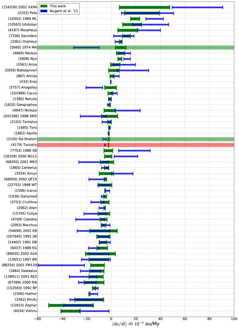
Figure 2: A comparison of our Yarkovsky detections (green) and those determined by Nugent et al. (2012) (blue), when we used all available data. Measurements that disagreed (i.e., $z_{i}>2$, Section 6) only when using all available data are highlighted in green, while those that also disagreed when matching observational intervals are highlighted in red. Objects are ranked from most positive to most negative Yarkovsky drift rate.

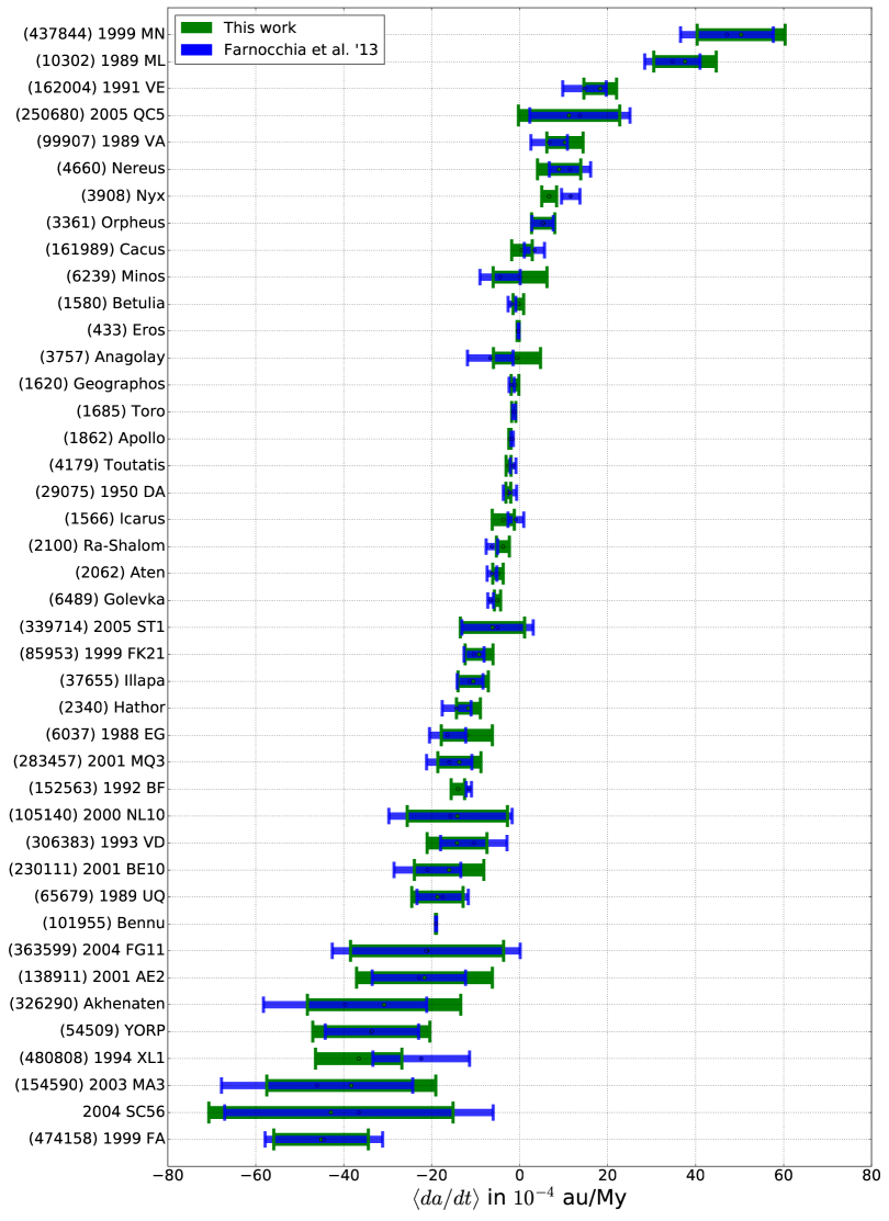
Figure 3: A comparison of our Yarkovsky detections (green) and those determined by Farnocchia et al. (2013) (blue), when we used matching data arcs. Some objects ((483656) 2005 ES70, 2003 XV, 2004 BG41, 2007 PB8, 2009 BD) were not included in this plot for display purposes, but all of them had $z_{i}<=2$. Objects are ranked from most positive to most negative Yarkovsky drift rate.

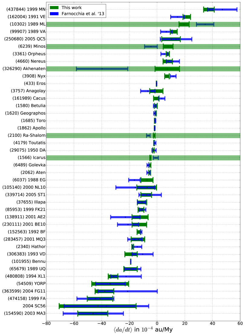
Figure 4: A comparison of our Yarkovsky detections (green) and those determined by Farnocchia et al. (2013) (blue), when we used all available data. Measurements that disagreed (i.e., $z_{i}>2$, Section 6) are highlighted in green. Some objects ((483656) 2005 ES70, 2003 XV, 2004 BG41, 2007 PB8, 2009 BD) were not included in this plot for display purposes, but all of them had $z_{i}<=2$. Objects are ranked from most positive to most negative Yarkovsky drift rate.

9 Comparison with Farnocchia et al. (2013)

9.0.1 Using matching observation intervals

We analyzed the 47 Yarkovsky objects found by Farnocchia et al. (2013) using matching observation intervals (to the nearest calendar year) and compared (Section 6) our results with their findings. We found agreement on all $\left\langle{da/dt}\right\rangle$ values (Figure 3).

We found that five objects – (1580) Betulia, , (326290) Akhenaten, (161989) Cacus, and 2003 XV – that were considered to be detections by Farnocchia et al. (2013) did not pass our detection threshold (Section 5.2). However, all five of these discrepant objects are listed in Tables 3 and 4 of Farnocchia et al. (2013), indicating that they are either “less reliable” detections or have low S/N values.

9.1 Using all available data

When using all available data, we found relatively good agreement (Figure 4). However, we found five objects — (2100) Ra-Shalom, (6239) Minos, (326290) Akhenaten — for which our drift rates do not match those of Farnocchia et al. (2013). We discuss these special cases in Section 13.6.

10 Yarkovsky efficiency distribution

Equations (3) and (4) provide a mechanism to interpret the drift in semi-major axis $\left\langle{da/dt}\right\rangle$ in terms of physical parameters of the measured object. In particular, $\left\langle{da/dt}\right\rangle$ can be described in terms of the Yarkovsky efficiency, $\xi$, where $0<\xi<1$. However, the relationship between $\left\langle{da/dt}\right\rangle$ and $\xi$ depends on density and diameter, and thus determination of $\xi$ requires estimation of these physical parameters.

Diameters were extracted from the Small Body Database (SBDB) (JPL Solar System Dynamics, 2019b, see also Section 12). Densities were assigned according to taxonomic types, which we also extracted from the SBDB, using the mean values reported by Carry (2012). Objects of unknown taxonomic type were assigned a density equal to the median density (2470 kg/m³) for the objects in our sample with known type.

We analyzed the distribution of $\xi$ values and found a median Yarkovsky efficiency of $\xi=0.12_{-0.06}^{+0.16}$ (Figure 5). Note that a bias in this estimate stems from our inability to report near-zero drift rates as Yarkovsky detections. Therefore, the true distribution of efficiencies is presumably shifted toward lower values than presented here.

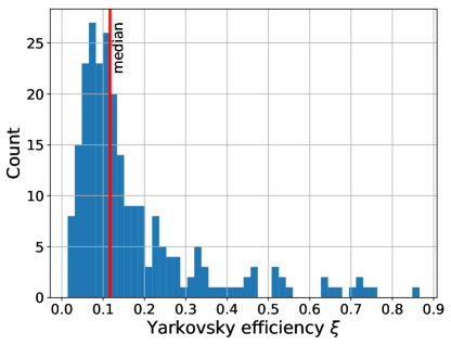
Figure 5: The distribution of Yarkovsky efficiencies $\xi$ measured with our sample of 247 objects. Diameter and density assumptions are described in the text. The median efficiency, $\xi=0.12$, is shown with a red vertical line. For clarity, we did not plot four objects with unphysical ($>$1) efficiencies (Section LABEL:sec-unphysical).

Several objects exhibit Yarkovsky efficiencies that substantially exceed the median value of $\xi=0.12$. For these objects, the nongravitational influence, if real, may be unrelated to Yarkovsky (e.g., sublimation). It is also possible that some of the high-efficiency detections are fictitious (e.g., faulty astrometry). For these reasons, we added a cautionary flag to 20 objects with Yarkovsky efficiencies above 0.5 in Table 1. We discuss the unphysical detections in Section LABEL:sec-unphysical.

11 Spin orientation distribution

La Spina et al. (2004) provided an estimate of the ratio of retrograde to prograde rotators ($N_{R}/N_{P}=2^{+1}_{-0.7}$) in the NEA population from a survey of spin vectors.

Measurements of the Yarkovsky drift rate can also be used to infer $N_{R}/N_{P}$, because objects with a positive $\left\langle{da/dt}\right\rangle$ are almost certain to be prograde rotators, while objects with a negative $\left\langle{da/dt}\right\rangle$ are almost certain to be retrograde rotators. This theorized correlation between drift rate and obliquity is borne out in all cases where both quantities can be estimated (Farnocchia et al., 2013).

However, given a population of objects with estimated $\left\langle{da/dt}\right\rangle$ values, the best estimate of $N_{R}/N_{P}$ is not equal to the ratio $R$ of the number of objects with negative $\left\langle{da/dt}\right\rangle$ to the number with positive $\left\langle{da/dt}\right\rangle$. A bias occurs because each estimated $\left\langle{da/dt}\right\rangle$ value has an associated uncertainty, and there is thus a nonzero probability that an object with a measured positive $\left\langle{da/dt}\right\rangle$ value in fact has a negative $\left\langle{da/dt}\right\rangle$ value (and vice versa). Because there are more retrograde rotators than prograde rotators, this process will bias observers toward measuring a lower observed ratio, $R_{O}$, than is actually present.

This point can be illustrated with a simple (albeit exaggerated) analytic example. Consider four objects: $A$, $B$, $C$, and $D$. Objects $A$, $B$, and $C$ all have $\left\langle{da/dt}\right\rangle$ values of $-10\pm 25\times 10^{-4}\text{ au/My}$, while object $D$ has an observed $\left\langle{da/dt}\right\rangle$ value of $+10\pm 25\times 10^{-4}\text{ au/My}$. In this example, the true ratio, $R_{T}$, of the number of objects with negative $\left\langle{da/dt}\right\rangle$ to the number of objects with positive $\left\langle{da/dt}\right\rangle$ is $R_{T}=3.0$. However, when an observer attempts to measure, for example, $\left\langle{da/dt}\right\rangle_{A}$, there is a $\sim$34% chance that the observer will erroneously conclude that $A$ has a positive $\left\langle{da/dt}\right\rangle$ value. In fact, we can calculate the probabilities associated with each of the five possible ratios that can be observed (Table 3) and demonstrate that one is most likely to observe $R_{O}=1.0$. If 10,000 observers independently took measurements of objects $A$, $B$, $C$, and $D$, a plurality would conclude that $R_{O}=1.00$, while a majority would agree that $R_{O}$ lies between 0.0 and 1.0 — even though the true ratio is $R_{T}=3.0$.

Table 3: The probability ($P$, rightmost column) of measuring a given ratio ($R_{O}$) of number of objects with $\left\langle{da/dt}\right\rangle<0$ ($N_{<0}$) to number of objects with $\left\langle{da/dt}\right\rangle>0$ ($N_{>0}$) for a sample of objects with true ratio $R_{T}=3.0$ (Section 11). The true ratio is not the most likely result for an observer to measure.

$N_{<0}$	$N_{>0}$	$R_{O}$	$P$
4	0	$\infty$	$10\%$
3	1	3.00	$34\%$
2	2	1.00	$37\%$
1	3	0.33	$17\%$
0	4	0.00	$3\%$

Our data suggest that out of 247 objects, 173 have $\left\langle{da/dt}\right\rangle<0$, for an observed ratio of $R_{O}=\frac{173}{247-173}=2.34$. To approximate the true ratio $R_{T}$, we assumed that the nominal ratio we measured was the most likely ratio for any observer to measure. Determining the true ratio is then a matter of simulating a universe with a set of simulated $\left\langle{da/dt}\right\rangle$ values that are consistent with our measured values, and also yield $R_{O}=2.34$.

To find the value of $R_{T}$ that corresponds to our measured $R_{O}$ value, we ran a set of nested Monte Carlo simulations, using the following procedure:

1. Create a new ‘universe’, $U_{i}$.

   1. Within $U_{i}$, generate a set of 247 $\left\langle{da/dt}\right\rangle$ values, pulled from distributions consistent with our measurements. This set of $\left\langle{da/dt}\right\rangle$ values are the true values for the 247 objects in universe $U_{i}$. Therefore, $R_{T}$ can be calculated (exactly) for this universe.

   2. Simulate what $10^{4}$ independent observers in universe $U_{i}$ would measure as an observed ratio, $R_{O}$.

   3. Determine the mean and standard deviation in observed ratio ($R_{O}$ and $\sigma_{R}$, respectively) in universe $U_{i}$ (Figure 6).

2. Repeat step 1 over many ($\sim$$10^{3}$) universes, and record the set of resulting distinct $R_{T}$ values, and corresponding $R_{O}$, $\sigma_{R}$ values.

3. Determine the set of $R_{T}$ values for which $R_{O}\pm\sigma_{R}$ encompasses our observed ratio of $R_{O}=2.34$.

The resulting simulations suggest that the most likely true ratio for our observed 247 objects is in the interval $R_{T}=2.29-2.69$, with a strong preference for the upper end of the interval, which corresponds to a 72% fraction of retrograde rotators in our sample.

Because our sample size is limited, we must also account for sampling errors, which will further broaden the uncertainties on $R$. The sampling uncertainty $\sigma_{S}$ on a measured ratio of $R$ from a sample of $N$ objects can be calculated directly from the standard deviation of the binomial distribution and is given by

$$\sigma_{S}\approx\sqrt{NR}\times\frac{R+1}{N-R}.$$ (11)

The sampling uncertainty for $R$ is therefore $\sigma_{S}=0.33$, which suggests a Yarkovsky-based estimate for the ratio of retrograde to prograde NEAs of

$$N_{R}/N_{P}=2.7^{+0.3}_{-0.7}.$$ (12)

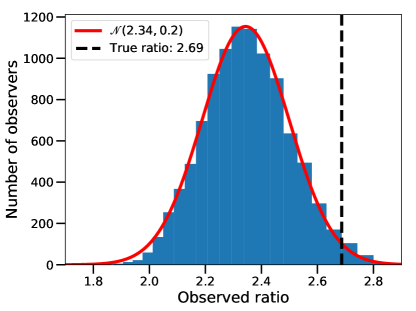
Figure 6: The number of observers measuring a given ratio $R_{O}$, for $10^{4}$ independent observers measuring 247 simulated objects with $\left\langle{da/dt}\right\rangle$ values consistent with what we measured (Section 11). For a true ratio of $R_{T}=2.69$, most observers will measure a ratio near $R_{O}=2.34$. This bias must be corrected for when estimating the ratio of retrograde to prograde rotators from Yarkovsky observations.

The ratio of retrograde to prograde rotators can in principle provide bounds on the fraction of NEAs that enter near-Earth space through the $\nu_{6}$ resonance (Nugent et al., 2012; Farnocchia et al., 2013). It is usually assumed that only retrograde rotators can escape through the $\nu_{6}$ resonance and that prograde and retrograde rotators have an equal probability of escaping through all other routes. With these assumptions, the fraction of objects that escape through the $\nu_{6}$ resonance can be evaluated as $f_{\nu_{6}}=(N_{R}/N_{P}-1)/(N_{R}/N_{P}+1)$. Our best estimate of the observed ratio (Equation 12) yields $f_{\nu_{6}}=46\%$. However, the NEA population model of Granvik et al. (2018) suggests that our sample contains a factor of 10 overrepresentation of Atens compared to their expected 3.5% fraction in the overall population, and therefore a much larger fraction of asteroids originating through the $\nu_{6}$ resonance, $f_{\nu_{6}}\sim 74\%$. If the population model predictions are correct and the traditional assumptions about the sense of rotation of NEAs originating from various main belt escape routes are correct, we would expect to observe a ratio of retrograde to prograde rotators $N_{R}/N_{P}\sim 6$, which is more than twice what we actually observe. Resolution of this serious discrepancy may involve one or more of the following factors: NEA population model predictions are flawed, assumptions about the sense of rotation of NEAs originating from various escape routes are incorrect, NEA spin orientations change on timescales that are short compared to NEA dynamical lifetimes, or an additional, unrecognized bias in our sample exists. Additional estimates of the ratio of retrograde to prograde rotators with more stringent detection requirements (lower $p$ values) or a larger sample of NEAs (independent of the Yarkovsky sensitivity metric $s_{Y}$) indicate that the observed and true ratio for the entire sample do not exceed 2.8. However, the observed ratios for subsets of objects with diameters $>$ 1 km do get larger and closer to the $N_{R}/N_{P}$ values predicted from the relevant $f_{\nu 6}$ estimates. This observation suggests that sub-kilometer-size objects are more prone to reorientation on short timescales.

12 Yarkovsky effect’s diameter dependence

Equations (3) and (4) illustrate the relationship between the magnitude of the Yarkovsky effect and the affected object’s physical parameters. In particular, the theoretical formulation of this effect predicts a $D^{-1.0}$ dependence. Verifying this dependence with our data serves as a check on the theoretical underpinnings of the effect and also validates our results.

We obtained diameter estimates for objects in our sample from the SBDB (JPL Solar System Dynamics, 2019b). For those objects with no listed diameter, we estimated the diameter from the object’s $H$ magnitude using

$$D=\frac{10^{-0.2H}}{\sqrt{p_{V}}}1329\text{ km},$$ (13)

where the geometric albedo, $p_{V}$, was extracted from the SBDB, if available, otherwise set to a value of 0.14 (Stuart & Binzel, 2004). If the uncertainty in diameter was available in the SBDB, we used it, otherwise we set the uncertainty to a third of the diameter.

Here we note that while the analytical formulation of our Yarkovsky force model includes parameters that are dependent on the physical properties of the affected object (Section 4), the actual fit itself is dependent only on dynamics. In other words, our fits measure only the overall magnitude of the Yarkovsky acceleration and are entirely agnostic about physical parameters such as diameter. Therefore, we can examine the Yarkovsky drift’s dependence on diameter independently from the determination of the magnitude of the drift itself, and be confident that we are not committing a petitio principii.

We fit a power law of the form

$$\left\langle{da/dt}\right\rangle=C\times D^{p},$$ (14)

to describe the relationship between the magnitude of the Yarkovsky effect and the object diameter. We used an Orthogonal Distance Regression (ODR) (Jones et al., 2001–) algorithm to perform this fit, due to the potential errors present in both the dependent ($\left\langle{da/dt}\right\rangle$) and independent ($D$) variables (Figure 7). The resulting fit gave a best-fit power-law slope of $p=-1.06\pm 0.05$. We verified the robustness of this result against the choice of diameter uncertainties, with values ranging from a fourth to two thirds of the diameter, and found consistent results. We also verified this result against different starting conditions on $p$.

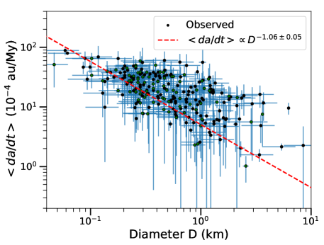
Figure 7: Drift rate $\left\langle{da/dt}\right\rangle$ as a function of object diameter, $D$. Diameters were either estimated from an $H$ magnitude (black) or extracted from the SBDB (green). Our analysis yields a diameter dependence of $D^{-1.06\pm 0.05}$, consistent with the theoretical expectation for the Yarkovsky effect of $D^{-1.0}$.

13 Objects of interest

13.1 (152563) 1992 BF

The 1992 BF astrometry includes four optical measurements taken in 1953. Vokrouhlický et al. (2008) showed that these points suffered from systematic errors due to faulty catalog debiasing and reanalyzed these measurements to determine more accurate values. We used these corrected data , and determined $\left\langle{da/dt}\right\rangle=(-13.2\pm 1.3)\times 10^{-4}\text{ au/My}$, which has a z-score of 1.69 with respect to Vokrouhlický et al. (2008)’s determination. The 1992 BF Yarkovsky drift was also measured with these points from 1953 discarded, which yielded $\left\langle{da/dt}\right\rangle=(-14.1\pm 2.3)\times 10^{-4}\text{ au/My}$.

13.2 2009 BD

Farnocchia et al. (2013) found a drift rate for 2009 BD of $\left\langle{da/dt}\right\rangle=(-493.4\pm 58.8)\times 10^{-4}\text{ au/My}$. Following the work of Micheli et al. (2012), Farnocchia et al. (2013) also fit for a Solar Radiation Pressure (SRP) model for this object – which introduces a radial acceleration as a function of Area-to-Mass Ratio (AMR) – and found AMR=$(2.72\pm 0.39)\times 10^{-4}$ m²/kg. Micheli et al. (2012) found AMR=$(2.97\pm 0.33)\times 10^{-4}$ m²/kg with a solution that did not include Yarkovsky.

We also included an SRP component in our force model for 2009 BD, and found an area-to-mass ratio of $(2.21\pm 0.40)\;\times 10^{-4}$ m²/kg, with a Yarkovsky drift rate of $\left\langle{da/dt}\right\rangle=(-497.6\pm 40.5)\times 10^{-4}\text{ au/My}$. The drastic improvement in goodness-of-fit when both Yarkovsky and SRP models are included (Table 4) strongly supports the presence of these forces. We note that while our uncertainties on the drift rate appear to be around 20% better than those of Farnocchia et al. (2013), this may be due to the method by which we fit for $\left\langle{da/dt}\right\rangle$, which was performed as a secondary minimization after fitting for the dynamical state vector. Therefore, our uncertainties in $\left\langle{da/dt}\right\rangle$ do not account for correlation between parameters and may be an underestimate because two related, nongravitational effects are present.

Table 4: Sum of squares of residuals ($\chi^{2}$) for 2009 BD, using various nongravitational dynamical models, with 190 total observations prior to outlier rejection. The inclusion of both Yarkovsky forces and Solar Radiation Pressure (SRP) yields both a significantly lower $\chi^{2}$, as well as a decrease in the number of outliers, $N_{\text{outliers}}$.

$Model$	$\chi^{2}$	$N_{\text{outliers}}$
Gravity-only	109	7
Yarkovsky	95	7
SRP	90	7
Yarkovsky+SRP	75	4

13.3 (483656) 2005 ES70

The drift in semi-major axis for 2005 ES70 is $\left\langle{da/dt}\right\rangle=(-79.6\pm 3.1)\times 10^{-4}\text{ au/My}$. Not only is this a strong effect, but it is also an unusually strong detection, with a $p$-value less than $10^{-16}$, and an S/N greater than 25. Farnocchia et al. (2013) found $\left\langle{da/dt}\right\rangle=(-55.6\pm 16.7)\times 10^{-4}\text{ au/My}$ using pre-2013 astrometry, which is consistent with our reanalysis of this object using the same arc ($\left\langle{da/dt}\right\rangle=(-54.1\pm 17.7)\times 10^{-4}\text{ au/My}$).

The drop in uncertainty by over a factor of five in six years is likely due to the increase in data coverage. This object has a total of 172 optical and a single Doppler measurement since its discovery in 2005. Of these epochs, 83 were measured after 2011 and were therefore not included in the analysis performed by Farnocchia et al. (2013). Thus, both the observational arc and the number of observations have doubled since 2011, which explains the drop in uncertainty.

The strength of this effect appears to be anomalous; however, when we account for this object’s small size, we find that its drift rate is reasonable. Specifically, the diameter of 2005 ES70 is $\sim$60 m, as calculated from an $H$ magnitude 23.8 (Equation 13), which corresponds to a Yarkovsky efficiency of $\xi=0.06$, assuming a density of 2470 kg/m³.

13.4 (1566) Icarus, (66146) 1998 TU3, (66391) Moshup, (137924) 2000 BD19, (364136) 2006 CJ, (437844) 1999 MN, and (480883) 2001 YE4

1Section previously titled: 13.4 (480883) 2001 YE4, (364136) 2006 CJ & (437844) 1999 MN

2006 CJ represents a strong Yarkovsky detection with $\left\langle{da/dt}\right\rangle=(-38.2\pm 1.8)\times 10^{-4}\text{ au/My}$.The relatively small uncertainty on this rate is largely due to radar observations. Our analysis includes 11 range and Doppler measurements of 2006 CJ from 2012 to 2017, and these points reduced the uncertainty on this detection by $\sim$85%.

With a drift rate of $\left\langle{da/dt}\right\rangle=(37.4\pm 3.8)\times 10^{-4}\text{ au/My}$, 1999 MN is notable not only for the high drift rate and S/N, but also for having a semi-major axis that is increasing rather than decreasing. Like the other objects in this section, 1999 MN’s small semi-major axis and large eccentricity result in a more pronounced drift rate. While this object’s drift rate is large, the Yarkovsky efficiency for 1999 MN is $\xi=0.05$, well within the nominal range.

2001 YE4 has among the largest drift rates in this data set, while also having amongst the smallest uncertainties, with $\left\langle{da/dt}\right\rangle=(-49.8\pm 0.7)\times 10^{-4}\text{ au/My}$. The small uncertainty is largely explained by the seven radar measurements over three ranging apparitions — an analysis of the drift that does not include these points yields $\left\langle{da/dt}\right\rangle=(-48.5\pm 2.0)\times 10^{-4}\text{ au/My}$, which means that the radar astrometry reduced the uncertainty by 65%. The drift rate, while large, corresponds to a Yarkovsky efficiency of $\xi=0.13$, which is close to the median efficiency for the objects we analyzed.

13.5 (4179) Toutatis

(4179) Toutatis is the only object in our sample for which our rate disagreed with a previous work’s result when using similar observation intervals – namely, our rate of $\left\langle{da/dt}\right\rangle=(-2.4\pm 0.8)\times 10^{-4}\text{ au/My}$ has a $z$-score of 2.7 when compared to Nugent et al. (2012)’s rate of $\left\langle{da/dt}\right\rangle=(-5.0\pm 0.6)\times 10^{-4}\text{ au/My}$. Our rate when using all available data, $\left\langle{da/dt}\right\rangle=(-2.15\pm 0.3)\times 10^{-4}\text{ au/My}$, is also not consistent with the previous work’s result.

Our rates do agree with Farnocchia et al. (2013), who found $\left\langle{da/dt}\right\rangle=(-1.5\pm 0.6)\times 10^{-4}\text{ au/My}$. Farnocchia et al. (2013) suggest that this object’s passage through the Main Belt may make its orbit particularly sensitive to the number and mass of gravitational perturbers.

Another curiosity surrounding Toutatis is the drastic change in drift rate that we found when including radar observations, compared to using only optical observations – including radar observations results in an apparent $\sim$80% drop in the calculated drift rate.

We found that the difference $\left\langle{da/dt}\right\rangle_{o}-\left\langle{da/dt}\right\rangle_{r+o}$ between Toutatis’s optical-only drift rate and the radar+optical drift rate is a strong function of the mass of the 24 Main Belt perturbing objects included in our force model. The perturbers included in our integration account for only $\sim$50% of the total mass of the Main Belt. Artificially increasing the overall mass of these perturbers brings the $\left\langle{da/dt}\right\rangle_{o}$ value into closer agreement with the $\left\langle{da/dt}\right\rangle_{r+o}$ value. An incomplete dynamical model may therefore explain the discrepancy between Toutatis’s optical-only rate and radar+optical rate.

A final peculiarity about Toutatis is that its orbit can be determined without any optical astrometry. We fit our gravity-only and Yarkovsky models to the 61 radar measurements obtained over six apparitions. The solutions are almost exactly the same as the solutions that include optical astrometry (Table 5). Furthermore, a trajectory fit using only radar data is consistent with optical data – the radar-only trajectory yields a sum of squares of residuals to optical data of $\chi_{\text{opt}}^{2}=2402$ with 12,070 measurements, i.e., an excellent reduced $\chi_{\text{opt},\nu}^{2}\sim$ 0.2.

These results suggest that the 61 radar observations over six apparitions are enough data to obtain a trajectory that is better than the one inferred from over 12,000 distinct optical measurements.

Table 5: Toutatis’s orbital elements at epoch 01-JAN-2000 12:00:00 TDT, as determined from radar+optical data, and differences in orbital element values obtained between the optical-only and radar+optical Yarkovsky solutions ($\Delta_{\text{o-only}}$), and between the radar-only and radar+optical Yarkovsky solutions ($\Delta_{\text{r-only}}$). The tiny deviations in the last column suggest that optical astrometry is not necessary to determine Toutatis’s orbit. Orbital elements include $i$, inclination with respect to J2000.0 ecliptic frame, $\Omega$, longitude of the ascending node, $\omega$, argument of pericenter, and $M$, mean anomaly at epoch. 1Numerical values in this table have been updated.

Orb. element	radar+optical	$\Delta_{\text{o-only}}$	$\Delta_{\text{r-only}}$
$a$ (au)	2.51054984474	1.4e-09	-1.8e-11
$e$	0.63428487023	-1.5e-09	-1.2e-10
$i$ (deg)	0.46970399148	-2.5e-07	2.5e-08
$\Omega$ (deg)	128.367186601	-6.5e-06	3.2e-06
$\omega$ (deg)	274.683232468	1.5e-06	-3.1e-06
$M$ (deg)	-76.1727086679	1.2e-06	-1.2e-08

13.6 (2100) Ra-Shalom, (5660) 1974 MA, (6239) Minos, (10302) 1989 ML, and (326290) Akhenaten

1Section previously titled: 13.6 (2100) Ra-Shalom, (326290) Akhenaten, and (6239) Minos

These objects are those for which we found statistically different results for the drift rate when comparing between our analysis with modern data and the analysis performed by Farnocchia et al. (2013) using pre-2013 data. Our drift rates do match Farnocchia et al. (2013)’s rates when using the same observational intervals (Section 9).

We found a drift rate of Ra-Shalom $\left\langle{da/dt}\right\rangle=(-2.04\pm 0.6)\times 10^{-4}\text{ au/My}$, while Farnocchia et al. (2013) found $\left\langle{da/dt}\right\rangle=(-6.31\pm 1.3)\times 10^{-4}\text{ au/My}$ using pre-2013 data. A total of 686 new optical observations have been added since 2013, resulting in a $\sim$50% increase in the size of the data set. The observations since 2013 also include the longest continuous set of observations ever taken for Ra-Shalom, of around five months, or $\sim$1/2 of an orbit (here we define a set of observations as continuous if there is no period spanning more than two weeks without at least one measurement within the set). Characterization of the Yarkovsky effect is aided by greater orbital coverage – therefore, we expect this modern set of observations to provide better constraints for this object than was previously possible.

For Minos, we find a rate of $\left\langle{da/dt}\right\rangle=(7.98\pm 3.54)\times 10^{-4}\text{ au/My}$, whereas Farnocchia et al. (2013) found $\left\langle{da/dt}\right\rangle=(-4.45\pm 4.57)\times 10^{-4}\text{ au/My}$ using pre-2013 data. The number of observations for this object has increased by over 50% since 2011, while the length of the observation interval has increased by 25%. The much larger data set explains our low $p$-value ($p=10^{-5}$), and the shift in the measured effect. We also note that Farnocchia et al. (2013) reported this object as a less confident detection, with S/N$<$2.

For Akhenaten, we found a drift rate of $\left\langle{da/dt}\right\rangle=(7.35\pm 8.8)\times 10^{-4}\text{ au/My}$, while Farnocchia et al. (2013) found $\left\langle{da/dt}\right\rangle=(-39.7\pm 18.6)\times 10^{-4}\text{ au/My}$ using pre-2013 data. Not only do these rates differ drastically in both magnitude and direction, but we also do not consider Akhenaten a Yarkovsky detection ($p=0.11$). There have been only 18 new observations of this object since 2012 (a $\sim$7% increase).

13.7 (1036) Ganymed

1Section previously titled: 13.7 (174050) 2002 CC19 and (1036) Ganymed

(1036) Ganymed is a large ($D\sim 37$ km) object that provides a good motivation to implement Yarkovsky drift rate validation tests that remove early astrometry. Our nominal solution yields an unphysical ($\xi=4.14$) Yarkovsky efficiency, which is too high to be explained by an uncertain density. Despite a $p$-value of $<10^{-16}$, our validation tests identified this detection as spurious. This object has measurements starting in 1924, and thus has one of the longest observational arcs we considered. It also has one of the largest sets of observations, $N_{o}=6359$. Nugent et al. (2012) found $\left\langle{da/dt}\right\rangle=(-6.6\pm 1.5)\times 10^{-4}\text{ au/My}$, consistent with our value ($\left\langle{da/dt}\right\rangle=(-5.0\pm 1.3)\times 10^{-4}\text{ au/My}$), and devoted a section in their article to this anomalous case. Farnocchia et al. (2013) determined a drift rate ($\left\langle{da/dt}\right\rangle=(-6.1\pm 1.6)\times 10^{-4}\text{ au/My}$) consistent with Nugent et al. (2012)’s and ours, but marked it as a potentially spurious detection, due to the unexpected strength of the drift rate relative to asteroid Bennu’s rate scaled for diameter. Both Nugent et al. (2012) and Farnocchia et al. (2013) suggested that this detection may be due to older, potentially faulty measurements introducing a false signal. Nugent et al. (2012) also explored the impact of an incorrect size or mass determination.

To examine the possibility that some of the Ganymed astrometry is faulty, we reran our Yarkovsky determination process after discarding observations prior to successively later starting dates (Figure 8). We found that the detected drift rate abruptly disappears if data prior to 1951 are discarded. This fact, combined with the unphysically large Yarkovsky efficiency implied by the large $\left\langle{da/dt}\right\rangle$, leads us to believe that this object’s drift rate has been artificially magnified by poor, early astrometry.

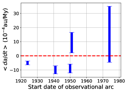
Figure 8: With a drift rate of $\left\langle{da/dt}\right\rangle=(-5.0\pm 1.3)\times 10^{-4}\text{ au/My}$, (1036) Ganymed appears to have an unphysical Yarkovsky efficiency of $\xi=4.12$. We find that if observations prior to 1950 are discarded, the Yarkovsky effect for this object appears to abruptly disappear. Ganymed may have an unreliably determined drift rate due to faulty older astrometry.

13.8 (99942) Apophis

1Section added at reviewer’s request.

Apophis has previously had a Yarkovsky drift detection of $\left\langle{da/dt}\right\rangle=(-23\pm 13)\times 10^{-4}\text{ au/My}$ (Vokrouhlický et al., 2015b). Apophis was not included in our list of candidates because it scores low (0.5) on the Yarkovsky sensitivity metric $s_{Y}$. However, an analysis of this object’s astrometry with our orbit determination software does indeed find a drift rate of $\left\langle{da/dt}\right\rangle=(-25.6\pm 13.6)\times 10^{-4}\text{ au/My}$, with a $p$-value of $10^{-9}$. This independently confirms the previous finding of Vokrouhlický et al. (2015b).

This result suggests that our initial screening can be overly restrictive by rejecting objects that do have detectable drift rates. An obvious solution would be to attempt detections of Yarkovsky rates for all NEAs, which is beyond the scope of this work.

13.9 Binary and triple asteroids

1Section previously titled: 13.8 Binary asteroids

Across our data sets, we considered a total of 44 numbered binary or triple asteroids. Among these, 18 have $p<0.05$ and 14 passed all our detection validations. These systems are flagged with a ^B in Table 1. Binaries present an opportunity to infer thermal properties from a Yarkovsky measurement, because tight constraints can be placed on both mass and obliquity for these objects (Section 14.3, Margot et al., 2015).

14 Discussion

14.1 Population-based detection verification

We have presented a statistical test that can be used to verify that a Yarkovsky detection is valid. However, one might still make the argument that the detections presented herein are merely due to statistical fluctuations. After all, the Yarkovsky effect often results in extremely small variations in an orbit. Perhaps the detections we present are really just a side effect of adding an extra degree of freedom to the gravity-only dynamical model.

Given the number of objects in our samples, we can address these concerns by looking for verifications of our detections on a population level, in addition to object by object. One such verification is the correspondence between the measured $\left\langle{da/dt}\right\rangle$ versus $D$ inverse relationship, and the relationship predicted by the Yarkovsky theory (Section 12). It seems unlikely that a process that is merely fitting for statistical noise would generate the $1/D$ behavior that we expect a priori.

Another population-level analysis considers the distribution of spin poles of NEAs. We have already discussed how we measured the ratio of retrograde to prograde rotators in our sample (Section 11). We can also use the raw number of negative $\left\langle{da/dt}\right\rangle$ values compared to positive $\left\langle{da/dt}\right\rangle$ values to test the “statistical noise hypothesis.” Namely, we can ask the following question: if our dynamical model, purportedly measuring a nongravitational force, were instead merely overfitting for statistical noise, what would be the probability that we would have measured the number of retrograde rotators that we saw in our sample? In other words, what is the probability $P$ of achieving a particular number $m$ (or more) of negatively signed $\left\langle{da/dt}\right\rangle$ values in a population of $N$ objects?

This question can be rephrased in terms of the probability $P$ of of observing at least $m$ heads after $N$ coin tosses, for a coin weighted with probability $p$. This can be answered using the binomial distribution

$$P=1-B(m-1,N,p).$$ (15)

In our sample, we have $m=173$ objects with a negative $\left\langle{da/dt}\right\rangle$ out of $N=247$ objects total. To determine $p$, we first assume that the nongravitational dynamical model is in fact overfitting for noise. In that case, the extraneous parameter would not favor one sign or another – in other words, the distribution of $\left\langle{da/dt}\right\rangle$ values that are measured should have a median of 0, which would suggest $p=0.5$.

The theoretical probability of observing 173 heads in 247 tosses of a fair coin is $\sim$10^-10 (Equation 15). In order to avoid making precise statements on the basis of a small sample, we report this probability as $P\ll 0.0001$. If the model were merely measuring statistical noise, the odds of finding the ratio of negatively signed to positively signed drift rates observed in our data set (or a ratio more extreme) is much less than 1 in $10^{4}$. This extremely low value provides an ab absurdo refutation of the hypothesis that we are fitting for noise. Note that this probability was calculated with minimal assumptions about the nature of the underlying statistical noise – we need only assume some distribution with a median of $\left\langle{da/dt}\right\rangle=0$.

14.2 The viability of Yarkovsky measurements

For those objects with previous Yarkovsky detections, we have compared results from two previous works (namely, Nugent et al. (2012) and Farnocchia et al. (2013)) and found excellent agreement (Section 6). The general strength and consistency of the agreement when using roughly similar observation intervals (where we found disagreement on drift rates for only a single object) serve as a validation of the methods employed by all three groups. The agreement when we used all data available to us (where we found disagreement on drift rates for only six objects) speaks to the viability of measuring this small effect from astrometric measurements, because the measured rates are stable, even with the addition of new data.

Among this work and the two previous studies, at least three different orbital integration packages were used to perform the analyses, indicating robustness of the results against numerical implementations.

14.3 Using the Yarkovsky efficiency $\xi$ to provide insights into NEA thermal properties

1Section previously titled: Interpreting $\xi$

We have found that within our sample of objects, typical Yarkovsky efficiencies lie between 0.06 and 0.27 (Section 10). An in-depth interpretation of these values would require a full thermal model of each object. However, we can still provide insights by making the simplifying assumption that all absorbed photons are reemitted equatorially. Then, the $\xi$ values can be interpreted relative to the obliquity and thermal properties of the object in one of three ways:

1. If all the reradiated photons were emitted at the same phase lag of $\phi=\pm 90^{\text{$\circ$}}$, then the obliquity would be $\gamma\sim\arccos{\xi}$. With these assumptions, our typical $\xi$ values suggest a range of obliquities 74${}^{\text{$\circ$}}<\gamma<87^{\text{$\circ$}}$ or $93^{\text{$\circ$}}<\gamma<$106${}^{\text{$\circ$}}$.

2. If the obliquity, $\gamma$, were $0^{\text{$\circ$}}$ or $180^{\text{$\circ$}}$, and all the reradiated photons were emitted at the same phase lag, then the phase lag would be $|\phi|\sim\arcsin{\xi}$. With these assumptions, typical efficiencies of $0.06<\xi<0.27$ imply phase lags of $3^{\text{$\circ$}}<|\phi|<$16${}^{\text{$\circ$}}$.

3. If the obliquity were $\gamma=0^{\text{$\circ$}}$ or $\gamma=180^{\text{$\circ$}}$, and the phase lag were $\phi=\pm 90^{\text{$\circ$}}$, then $\xi$ could be interpreted as a measure of the distribution of photons that are emitted around $\phi$.

Item (1) seems unlikely, given that we expect most of these objects to have obliquities near $0^{\text{$\circ$}}$ or $180^{\text{$\circ$}}$ – Hanuš et al. (2013) found that among a sample of 38 NEAs, more than 70% had $\gamma<30^{\text{$\circ$}}$ or $\gamma>150^{\text{$\circ$}}$. Item (2) is more palatable, and its applicability is protected by the cosine function’s slow drop-off, which means that assuming very high or very low spin pole latitudes will introduce errors of less than 10% for those objects with $\gamma<30^{\text{$\circ$}}$ or $\gamma>150^{\text{$\circ$}}$.

Rubincam (1995) derived an expression for phase lag as a function of the thermal inertia $\Gamma$ of a body rotating at frequency $\nu$, and found

$$\phi=\text{arctan}\left(\frac{\Gamma\sqrt{\nu}}{\Gamma\sqrt{\nu}+\sqrt{32}\sigma T_{0}^{3}}\right),$$ (16)

where $\sigma$ is the Stefan-Boltzmann constant, and $T_{0}$ is the temperature of the body when it is at a distance $a$ from the Sun.

With a typical thermal inertia of $\Gamma=200$ J m^-2 s${}^{-\frac{1}{2}}$ K^-1 (Delbo et al., 2007), Equation (16) yields a phase lag of $\phi=8.7^{\text{$\circ$}}$ for a body orbiting at a distance of 1 au and rotating with a period of 4.5 hours. Assuming $\gamma=0^{\text{$\circ$}}$ or $\gamma=180^{\text{$\circ$}}$, our median Yarkovsky efficiency of $\xi=0.12$ suggests $|\phi|=7^{\text{$\circ$}}$, which is in good agreement with the phase lag derived from thermal properties. With a more complete thermal model, it should be possible to relate any of the differences between these two determinations to the distribution of reemitted photons (Item (3) above).

Better knowledge of $\gamma$ and $\xi$ will yield tighter constraints on thermal properties of NEAs. In particular, the obliquity and mass of binaries can be accurately determined through dynamical measurements of the system. Therefore, binaries with Yarkovsky estimates (Section 13.9) will likely provide the best constraints on thermal properties in the future.

14.4 Expected diameter dependence

Delbo et al. (2007) suggested that, due to a dependence between thermal inertia, $\Gamma$, and diameter, one might expect a flatter $\left\langle{da/dt}\right\rangle$ diameter dependence than predicted by a theory that disregards correlation between these parameters. In particular, they found that

$$\Gamma\propto D^{-p},$$ (17)

where $p$$\sim$$0.4$.

Delbo et al. (2007), citing Vokrouhlický (1999), wrote

$$\left\langle{da/dt}\right\rangle\propto D^{-1}\frac{\Theta}{1+\Theta+0.5\Theta^{2}},$$ (18)

where

$$\Theta =\frac{\Gamma}{\epsilon\sigma(\sqrt{2}T_{\text{0}})^{3}}\sqrt{\frac{2\pi}{P}},$$ (19)

where $\sigma$ is the Stefan-Boltzmann constant, $P$ is the rotation period, $\epsilon$ is the thermal emissivity, and $T_{0}$ is the temperature of the body when it is at a distance $a$ from the Sun.

Delbo et al. (2007) suggested that because the asymptotic behavior (i.e., $\Theta\gg 1$) of Equation (18) gives

$$\left\langle{da/dt}\right\rangle\propto D^{-1}\Theta^{-1},$$ (20)

then, by relating Equations (17), (19), and (20), one would find

$$\left\langle{da/dt}\right\rangle \propto D^{-1+p}\propto D^{-0.6}.$$ (21)

However, few objects yield values for $\Theta$ such that Equation (20)’s prerequisite of $\Theta\gg 1$ is appropriate. For example, typical objects in our sample have $P=4.5$ hours and $T_{0}=300$ K. With typical thermal inertias in the range $\Gamma\sim 200-400$ J m^-2 s^-0.5 K^-1, Equation (19) yields $\Theta\sim 1-2$. In fact, because Equation (18) peaks at $\Theta=1.4$, the slope of the function with respect to $\Theta$ near $\Theta=1-2$ is nearly 0, which suggests $\left\langle{da/dt}\right\rangle\propto D^{-1}\Theta^{0}\propto D^{-1}$.

We find $\left\langle{da/dt}\right\rangle\propto D^{-1.06\pm 0.05}$ (Section 12), which is consistent with the nominal theory.

14.5 Drift determination and radar ranging

While the Yarkovsky effect can be measured for objects with no radar ranging data, range astrometry aids greatly in improving the accuracy of drift determination. In particular, the number of distinct radar apparitions with range data correlates strongly with reduced uncertainty in an object’s drift rate.

Of the 247 objects we analyzed, 91 had radar astrometry. Of these, 76 objects had range measurements. We examined the improvement in the Yarkovsky determination – quantified by $\sigma_{\text{o}}/\sigma_{\text{r+o}}$, or the ratio of the drift uncertainty without radar to that with radar – compared to the number of radar range apparitions for that object (Figure 9). Although the exact trend is obscured by small number statistics, the improvement in precision appears to scale roughly as $2^{N_{\rm rad}-1}$, where $N_{\rm rad}$ is the number of apparitions with ranging data.

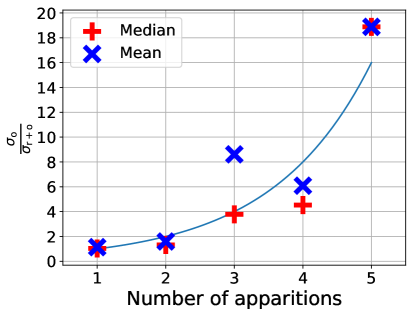
Figure 9: The ratio of the drift uncertainty without radar to that with radar, $\sigma_{\text{o}}/\sigma_{\text{r+o}}$, as a function of the number of radar apparitions during which ranging data were taken. The number of objects with radar range measurements were 43, 18, 10, 4, and 1, for 1, 2, 3, 4, and 5 apparitions, respectively.

15 Conclusion

With new astrometry and improved methods, we found a set of 247 NEAs with a measurable Yarkovsky drift. We found generally good agreement with previous studies. Most NEAs exhibit Yarkovsky efficiencies in a relatively small (0–0.2) range. We verified the Yarkovsky drift rate’s inverse dependence on asteroid size, and we estimated the ratio of retrograde to prograde rotators in the NEA population. In addition, we provided an estimate of the improvement in Yarkovsky determinations with the availability of radar data at multiple apparitions. Our results provide compelling evidence for the existence of a nongravitational influence on NEA orbits.

16 Acknowledgements

We are grateful for the help and insights provided by Alec Stein regarding the statistical analyses of our data.

AHG and JLM were funded in part by NASA grant NNX14AM95G and NSF grant AST-1109772. The Arecibo Planetary Radar Program is supported by the National Aeronautics and Space Administration under grant Nos. NNX12AF24G and NNX13AQ46G issued through the Near-Earth Object Observations program. This work was enabled in part by the Mission Operations and Navigation Toolkit Environment (MONTE). MONTE is developed at the Jet Propulsion Laboratory, which is operated by Caltech under contract with NASA. The material presented in this article represents work supported in part by NASA under the Science Mission Directorate Research and Analysis Programs.

References

- Becker et al. (2015) Becker, T. M., Howell, E. S., Nolan, M. C., et al. 2015, Icarus, 248, 499
- Bottke et al. (2006) Bottke, Jr., W. F., Vokrouhlický, D., Rubincam, D. P., & Nesvorný, D. 2006, Annual Review of Earth and Planetary Sciences, 34, 157
- Brozović et al. (2011) Brozović, M., Benner, L. A. M., Taylor, P. A., et al. 2011, Icarus, 216, 241
- Carry (2012) Carry, B. 2012, Planet. Space Sci., 73, 98
- Chesley et al. (2015) Chesley, S., Farnocchia, D., Pravec, P., & Vokrouhlicky, D. 2015, IAU General Assembly, 22, 2248872
- Chesley et al. (2010) Chesley, S. R., Baer, J., & Monet, D. G. 2010, Icarus, 210, 158
- Chesley et al. (2008) Chesley, S. R., Vokrouhlický, D., Ostro, S. J., et al. 2008, in Asteroids, Comets, Meteors 2008, Vol. 1405, 8330
- Delbo et al. (2007) Delbo, M., dell’Oro, A., Harris, A. W., Mottola, S., & Mueller, M. 2007, Icarus, 190, 236
- Evans et al. (2018) Evans, S., Taber, W., Drain, T., et al. 2018, CEAS Space Journal, 10, 79
- Fang & Margot (2012) Fang, J., & Margot, J. L. 2012, AJ, 143, 24
- Fang et al. (2011) Fang, J., Margot, J. L., Brozovic, M., et al. 2011, AJ, 141, 154
- Farnocchia et al. (2015) Farnocchia, D., Chesley, S. R., Chamberlin, A. B., & Tholen, D. J. 2015, Icarus, 245, 94
- Farnocchia et al. (2013) Farnocchia, D., Chesley, S. R., Vokrouhlický, D., et al. 2013, Icarus, 224, 1
- Folkner et al. (2014) Folkner, W. M., Williams, J. G., Boggs, D. H., Park, R. S., & Kuchynka, P. 2014, Interplanetary Network Progress Report, 196, 1
- Granvik et al. (2018) Granvik, M., Morbidelli, A., Jedicke, R., et al. 2018, Icarus, 312, 181
- Greenberg et al. (2017) Greenberg, A. H., Margot, J. L., Verma, A. K., et al. 2017, AJ, 153, 108
- Hanuš et al. (2013) Hanuš, J., Brož, M., Durech, J., et al. 2013, AAp, 559, A134
- Jones et al. (2001–) Jones, E., Oliphant, T., Peterson, P., et al. 2001–
- JPL Solar System Dynamics (2019a) JPL Solar System Dynamics. 2019a
- JPL Solar System Dynamics (2019b) —. 2019b
- Kelly (2007) Kelly, B. C. 2007, ApJ, 665, 1489
- La Spina et al. (2004) La Spina, A., Paolicchi, P., Kryszczyńska, A., & Pravec, P. 2004, Nature, 428, 400
- Lowry et al. (2007) Lowry, S. C., Fitzsimmons, A., Pravec, P., et al. 2007, Science, 316, 272
- Mandel (1964) Mandel, J. 1964, The Statistical Analysis of Experimental Data (Dover Publications)
- Margot (2004) Margot, J. L. 2004, in AAS/Division for Planetary Sciences Meeting Abstracts #36, 12.02
- Margot & Giorgini (2010) Margot, J. L., & Giorgini, J. D. 2010, in IAU Symposium, Vol. 261, IAU Symposium, ed. S. A. Klioner, P. K. Seidelmann, & M. H. Soffel, 183–188
- Margot et al. (2002) Margot, J. L., Nolan, M. C., Benner, L. A. M., et al. 2002, Science, 296, 1445
- Margot et al. (2015) Margot, J. L., Pravec, P., Taylor, P., Carry, B., & Jacobson, S. 2015, in Asteroids IV, ed. P. Michel, F. E. DeMeo, & W. F. Bottke (Univ. of Arizona Press), 355–373
- Meyers (2017) Meyers, J. 2017
- Micheli et al. (2012) Micheli, M., Tholen, D. J., & Elliott, G. T. 2012, NA, 17, 446
- Minor Planet Center (2019) Minor Planet Center. 2019
- Mommert et al. (2014) Mommert, M., Hora, J. L., Farnocchia, D., et al. 2014, ApJ, 786, 148
- Naidu et al. (2015) Naidu, S. P., Margot, J. L., Taylor, P. A., et al. 2015, AJ, 150, 54
- Nugent et al. (2012) Nugent, C. R., Margot, J. L., Chesley, S. R., & Vokrouhlický, D. 2012, Astronomical Journal, 144, 60
- Ostro et al. (2006) Ostro, S. J., Margot, J. L., Benner, L. A. M., et al. 2006, Science, 314, 1276
- Pravec et al. (2006) Pravec, P., Scheirich, P., Kušnirák, P., et al. 2006, Icarus, 181, 63
- Rubincam (1995) Rubincam, D. P. 1995, JGR, 100, 1585
- Scheeres et al. (2006) Scheeres, D. J., Fahnestock, E. G., Ostro, S. J., et al. 2006, Science, 314, 1280
- Scheirich et al. (2015) Scheirich, P., Pravec, P., Jacobson, S. A., et al. 2015, Icarus, 245, 56
- Springmann et al. (2014) Springmann, A., Taylor, P. A., Nolan, M. C., et al. 2014, in AAS/Division for Planetary Sciences Meeting Abstracts #46, 409.02
- Stuart & Binzel (2004) Stuart, J. S., & Binzel, R. P. 2004, Icarus, 170, 295
- Taylor et al. (2007) Taylor, P. A., Margot, J. L., Vokrouhlický, D., et al. 2007, Science, 316, 274
- Verma et al. (2017) Verma, A. K., Margot, J.-L., & Greenberg, A. H. 2017, ApJ, 845, 166
- Vokrouhlický (1999) Vokrouhlický, D. 1999, A&A, 344, 362
- Vokrouhlický et al. (2015a) Vokrouhlický, D., Bottke, W. F., Chesley, S. R., Scheeres, D. J., & Statler, T. S. 2015a, in Asteroids IV, ed. P. Michel, F. E. DeMeo, & W. F. Bottke (Univ. of Arizona Press), 509–531
- Vokrouhlický et al. (2008) Vokrouhlický, D., Chesley, S. R., & Matson, R. D. 2008, AJ, 135, 2336
- Vokrouhlický et al. (2015b) Vokrouhlický, D., Farnocchia, D., Čapek, D., et al. 2015b, Icarus, 252, 277
- Vokrouhlický et al. (2000) Vokrouhlický, D., Milani, A., & Chesley, S. R. 2000, Icarus, 148, 118
- Vokrouhlický et al. (2005) Vokrouhlický, D., Čapek, D., Chesley, S. R., & Ostro, S. J. 2005, Icarus, 179, 128