Magnon Dispersion and Specific Heat of Chiral Magnets on the Pyrochlore Lattice

Abstract

Chiral magnets are magnetically ordered insulators having spin scalar chirality, and magnons of chiral magnets have been poorly understood. We study the magnon dispersion and specific heat for four chiral magnets with $\bm{Q}=\bm{0}$ on the pyrochlore lattice. This study is based on the linear-spin-wave approximation for the $S=\frac{1}{2}$ effective Hamiltonian consisting of two kinds of Heisenberg interaction and two kinds of Dzyaloshinsky-Moriya interaction. We show that the three-in-one-out type chiral magnets possess an optical branch of the magnon dispersion near $\bm{q}=\bm{0}$, in addition to three quasiacoustic branches. This differs from the all-in/all-out type chiral magnets, which possess four quasiacoustic branches. We also show that all four chiral magnets have a gapped magnon energy at $\bm{q}=\bm{0}$, indicating the absence of the Goldstone type gapless excitation. These results are useful for experimentally identifying the three-in-one-out or all-in/all-out type chiral order. Then, we show that there is no qualitative difference in the specific heat among the four magnets. This indicates that the specific heat is not useful for distinguishing the kinds of chiral orders. We finally compare our results with experiments and provide a proposal for the three-in-one-out type chiral magnets.

1 Introduction

Magnons are bosonic quasiparticles describing the low-energy properties of a magnetically ordered system [1, 2]. A magnetically ordered system has a finite expectation value of some component of the spin at each site. The effects of the spin fluctuations can be described in terms of the bosonic operators because the spin operators can be expressed in terms of those using the Holstein-Primakoff transformation [3, 4, 5]. Since these bosonic operators describe the creation and annihilation of a magnon and the spin Hamiltonian is expressed in terms of these magnon operators, magnons describe the low-energy properties of a magnet. Note that the zeroth-order terms of the magnon operators describe the zero-point motion, the second-order terms describe the noninteracting magnons, and the higher-order terms describe the interactions between magnons.

Comparing with the understanding of magnons of nonchiral magnets, the low-temperature properties of magnons of chiral magnets are poorly understood. A chiral magnet is a magnetically ordered insulator with spin scalar chirality, while a nonchiral magnet does not have spin scalar chirality. (Our definition is distinct from another definition, in which a magnet on a chiral lattice is a chiral magnet, because our definition is applicable to even a nonchiral lattice, such as the pyrochlore lattice.) It is widely known [6, 7] that a major difference between collinear ferromagnetic (FM) and antiferromagnetic (AF) magnets, typical nonchiral magnets, is the different curvature of the magnon dispersion in the long-wavelength limit, and this curvature difference causes a difference in the temperature dependence of some quantity, such as the specific heat. However, such knowledge about chiral magnets is unsatisfactory even for noninteracting magnons. Thus, a detailed theoretical analysis of the chiral magnets may be needed.

To understand the properties of magnons of chiral magnets, we focus on $S=\frac{1}{2}$ pyrochlore magnets, magnetically ordered insulators on the pyrochlore lattice [8] (Fig. 1) with $S=\frac{1}{2}$ per site. The pyrochlore magnets can be chiral, depending on the values of exchange interactions. Examples of chiral magnets are all-in/all-out (AIAO) [9] and three-in-one-out (3I1O) ones [10]; their spin structures are shown in Fig. 2. Although the magnon properties of the AIAO chiral magnet have been revealed [9], it is unclear how they differ from magnon properties of other chiral magnets, and what property is characteristic of chiral magnets. It is thus desirable to clarify differences and similarities between magnons of the AIAO type and 3I1O type chiral magnets.

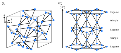
Figure 1: (Color online) (a) Pyrochlore lattice consisting of B ions in A₂B₂O₇ or AB₂O₄, and (b) the lattice as alternating kagome and triangle layers along the $[111]$ direction. Blue circles represent B ions, and $1$, $2$, $3$, and $4$ denote sublattices 1, 2, 3, and 4, respectively.

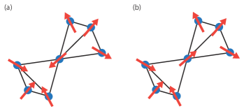
Figure 2: (Color online) Spin structures of (a) the AIAO and (b) 3I1O chiral magnets. Their ordering vectors are $\bm{Q}=\bm{0}$.

In this paper, we study the low-temperature properties of noninteracting magnons of $S=\frac{1}{2}$ pyrochlore magnets using the linear-spin-wave approximation (LSWA) [11, 12]. We consider several chiral magnets with $\bm{Q}=\bm{0}$, where $\bm{Q}$ is the ordering vector. We show that the 3I1O type chiral magnets possess an optical branch of the magnon dispersion near $\bm{q}=\bm{0}$, in addition to three quasiacoustic branches, while the four branches in the AIAO type chiral magnets are all quasiacoustic. We also show that the magnon energy at $\bm{q}=\bm{0}$ has a finite gap for the AIAO type and the 3I1O type chiral magnets.

Then, we show the results for the ground state of $S=\frac{1}{2}$ pyrochlore magnets using the mean-field approximation (MFA) for several chiral or nonchiral orders with $\bm{Q}=\bm{0}$. This is because the ground state determined in the MFA is a starting point to include the effects of fluctuations.

We organize this paper as follows. In Sect. 2, we explain our method for chiral magnets with $\bm{Q}=\bm{0}$ in pyrochlore oxides with weak spin-orbit coupling (SOC). In Sect. 3, we show the results obtained using the MFA and the LSWA. In Sect. 4, we discuss the applicability of the LSWA and the correspondences between our results and several experimental results, and propose several observable aspects for future experiments. In Sect. 5, we summarize our main results.

2 Method

In this section, we show our low-energy effective model for the $S=\frac{1}{2}$ pyrochlore oxides with weak SOC, and explain the MFA and the LSWA. In Sect. 2.1, we introduce the spin Hamiltonian consisting of the Heisenberg and Dzyaloshinsky-Moriya (DM) interactions between nearest-neighbor (NN) B ions on the pyrochlore lattice. In Sect. 2.2, we formulate the MFA for our spin Hamiltonian and explain how to determine the ground state. In Sect. 2.3, we formulate the LSWA for a commensurate magnetic order and then show an algorithm to obtain numerical solutions of the LSWA. Throughout this paper, we set $\hbar=1$ and $k_{\textrm{B}}=1$.

2.1 Model

As an effective Hamiltonian for the $S=\frac{1}{2}$ pyrochlore magnets, we use the following spin Hamiltonian [13]:

$$\hat{H}_{\textrm{eff}}= \sum\limits_{\langle\bm{i},\bm{j}\rangle}J_{\bm{i}\bm{j}}\hat{\bm{S}}_{\bm{i}}\cdot\hat{\bm{S}}_{\bm{j}}+\sum\limits_{\langle\bm{i},\bm{j}\rangle}\bm{D}_{\bm{i}\bm{j}}\cdot(\hat{\bm{S}}_{\bm{i}}\times\hat{\bm{S}}_{\bm{j}})$$

$$= \sum\limits_{m,n=1}^{N}\sum\limits_{l,l^{\prime}=1}^{4}\sum\limits_{\alpha,\beta=x,y,z}M_{mlnl^{\prime}}^{\alpha\beta}\hat{S}_{\bm{R}_{m}+\bm{r}_{l}}^{\alpha}\hat{S}_{\bm{R}_{n}+\bm{r}_{l^{\prime}}}^{\beta}.$$ (1)

Here $\bm{i}$ and $\bm{j}$ are site indices, $\bm{R}_{m}$ and $\bm{R}_{n}$ are translational vectors, $\bm{r}_{l}$ and $\bm{r}_{l^{\prime}}$ are sublattice vectors [i.e., $\bm{r}_{1}={}^{t}(0\ 0\ 0)$, $\bm{r}_{2}={}^{t}(\frac{1}{2}\ \frac{1}{2}\ 0)$, $\bm{r}_{3}={}^{t}(0\ \frac{1}{2}\ \frac{1}{2})$, and $\bm{r}_{4}={}^{t}(\frac{1}{2}\ 0\ \frac{1}{2})$], and $J_{\bm{i}\bm{j}}$ and $\bm{D}_{\bm{i}\bm{j}}$ are the Heisenberg and DM interactions between the NN B sites, respectively. $J_{\bm{i}\bm{j}}=J_{\bm{j}\bm{i}}$ and $\bm{D}_{\bm{i}\bm{j}}=-\bm{D}_{\bm{j}\bm{i}}$ are given by

$$J_{\bm{1}\bm{2}}=J_{0}+J_{1},\bm{D}_{\bm{1}\bm{2}}=\left(\begin{array}[]{@{\,}c@{\,}}-D_{0}-D_{1}\\ +D_{0}+D_{1}\\ 0\end{array}\right),$$ (5)

$$J_{\bm{1}\bm{3}}=J_{0}+J_{1},\bm{D}_{\bm{1}\bm{3}}=\left(\begin{array}[]{@{\,}c@{\,}}0\\ -D_{0}-D_{1}\\ +D_{0}+D_{1}\end{array}\right),$$ (9)

$$J_{\bm{1}\bm{4}}=J_{0}+J_{1},\bm{D}_{\bm{1}\bm{4}}=\left(\begin{array}[]{@{\,}c@{\,}}+D_{0}+D_{1}\\ 0\\ -D_{0}-D_{1}\end{array}\right),$$ (13)

$$J_{\bm{4}\bm{3}}=J_{0}-J_{1},\bm{D}_{\bm{4}\bm{3}}=\left(\begin{array}[]{@{\,}c@{\,}}+D_{0}-D_{1}\\ +D_{0}-D_{1}\\ 0\end{array}\right),$$ (17)

$$J_{\bm{2}\bm{4}}=J_{0}-J_{1},\bm{D}_{\bm{2}\bm{4}}=\left(\begin{array}[]{@{\,}c@{\,}}0\\ +D_{0}-D_{1}\\ +D_{0}-D_{1}\end{array}\right),$$ (21)

$$J_{\bm{2}\bm{3}}=J_{0}-J_{1},\bm{D}_{\bm{2}\bm{3}}=\left(\begin{array}[]{@{\,}c@{\,}}-D_{0}+D_{1}\\ 0\\ -D_{0}+D_{1}\end{array}\right).$$ (25)

The above $\bm{D}_{\bm{i}\bm{j}}$ are consistent with the Moriya rule [14, 15].

In our effective model, we consider not only the $J_{0}$ and $D_{0}$ terms but also the $J_{1}$ and $D_{1}$ terms for the following four reasons. First, the model only with the $J_{1}$ and $D_{1}$ terms is a minimal model for the 3I1O chiral magnet. The 3I1O chiral magnet is the most stable ground state in the minimal model for the negative $J_{1}$ and $D_{1}$ (see Table II). Second, the magnon properties obtained in the minimal model may remain qualitatively unchanged in a more realistic model for the 3I1O chiral magnet. Third, the model with the $J_{0}$, $D_{0}$, $J_{1}$, and $D_{1}$ terms is useful for analyzing the magnon properties of another chiral magnet whose spin structure is similar to that of the AIAO or 3I1O chiral magnet. A chiral magnet similar to the AIAO one is a distorted AIAO (dAIAO) chiral magnet, and a chiral magnet similar to the 3I1O one is a distorted 3I1O (d3I1O) chiral magnet (see Table III). Such analyses are useful for understanding magnon properties of the AIAO type and 3I1O type chiral magnets. Fourth, the values of the $J_{1}$ and $D_{1}$ terms may be controllable, for example, by varying the pressure along the $[111]$ direction.

2.2 Mean-field approximation

We start with the formulation of the MFA. In the MFA, we neglect fluctuations and replace one of the two spin operators in the Hamiltonian by the expectation value. Thus, the ground state in the MFA is given by

$$\langle\hat{H}_{\textrm{eff}}\rangle= \sum\limits_{m,n=1}^{N}\sum\limits_{l,l^{\prime}=1}^{4}\sum\limits_{\alpha,\beta}M_{mlnl^{\prime}}^{\alpha\beta}\langle\hat{S}_{\bm{R}_{m}+\bm{r}_{l}}^{\alpha}\rangle\langle\hat{S}_{\bm{R}_{n}+\bm{r}_{l^{\prime}}}^{\beta}\rangle.$$ (26)

In the above equation, $\langle\hat{\bm{S}}_{\bm{i}}\rangle$ should satisfy the hard-spin constraint, i.e., $S=\frac{1}{2}=|\langle\hat{\bm{S}}_{\bm{i}}\rangle|$. Since Eq. (26) can be expressed as a hermitian form in terms of the Fourier coefficients of $\langle\hat{S}^{\alpha}_{\bm{i}}\rangle$ and $\langle\hat{S}^{\beta}_{\bm{j}}\rangle$,

$$\langle\hat{H}_{\textrm{eff}}\rangle=\sum\limits_{\bm{q}}\sum\limits_{l,l^{\prime}=1}^{4}\sum\limits_{\alpha,\beta}M_{ll^{\prime}}^{\alpha\beta}(\bm{q})\langle\hat{S}_{\bm{q}l^{\prime}}^{\beta}\rangle\langle\hat{S}_{\bm{q}l}^{\alpha}\rangle^{\ast},$$ (27)

the determination of the ground state is equivalent to the determination of the minimum of $\langle\hat{H}_{\textrm{eff}}\rangle$ as a function of $\bm{q}$ under the hard-spin constraint. In Eq. (27), we have introduced $M_{ll^{\prime}}^{\alpha\beta}(\bm{q})=M_{l^{\prime}l}^{\beta\alpha}(\bm{q})$ [$M_{ll}^{\alpha\beta}(\bm{q})=0$], given by

$$M_{21}^{\alpha\beta}(\bm{q})=Z_{+}^{\alpha\beta}\cos(\frac{q_{x}}{2}+\frac{q_{y}}{2}),$$ (28)

$$M_{43}^{\alpha\beta}(\bm{q})=Z_{-}^{\alpha\beta}\cos(\frac{q_{x}}{2}-\frac{q_{y}}{2}),$$ (29)

$$M_{31}^{\alpha\beta}(\bm{q})=X_{+}^{\alpha\beta}\cos(\frac{q_{y}}{2}+\frac{q_{z}}{2}),$$ (30)

$$M_{42}^{\alpha\beta}(\bm{q})=X_{-}^{\alpha\beta}\cos(\frac{q_{y}}{2}-\frac{q_{z}}{2}),$$ (31)

$$M_{41}^{\alpha\beta}(\bm{q})=Y_{+}^{\alpha\beta}\cos(\frac{q_{z}}{2}+\frac{q_{x}}{2}),$$ (32)

$$M_{32}^{\alpha\beta}(\bm{q})=Y_{-}^{\alpha\beta}\cos(\frac{q_{z}}{2}-\frac{q_{x}}{2}),$$ (33)

with

$$Z_{\pm}^{\alpha\beta}=\begin{cases}J_{0}\pm J_{1}&\textrm{for}\ \alpha=\beta\\ D_{0}\pm D_{1}&\textrm{for}\ (\alpha,\beta)=(y,z)\\ \pm D_{0}+D_{1}&\textrm{for}\ (\alpha,\beta)=(x,z)\\ -(D_{0}\pm D_{1})&\textrm{for}\ (\alpha,\beta)=(z,y)\\ -(\pm D_{0}+D_{1})&\textrm{for}\ (\alpha,\beta)=(z,x)\end{cases},$$ (34)

$$X_{\pm}^{\alpha\beta}=\begin{cases}J_{0}\pm J_{1}&\textrm{for}\ \alpha=\beta\\ D_{0}\pm D_{1}&\textrm{for}\ (\alpha,\beta)=(y,x)\\ \pm D_{0}+D_{1}&\textrm{for}\ (\alpha,\beta)=(z,x)\\ -(D_{0}\pm D_{1})&\textrm{for}\ (\alpha,\beta)=(x,y)\\ -(\pm D_{0}+D_{1})&\textrm{for}\ (\alpha,\beta)=(x,z)\end{cases},$$ (35)

$$Y_{\pm}^{\alpha\beta}=\begin{cases}J_{0}\pm J_{1}&\textrm{for}\ \alpha=\beta\\ D_{0}\pm D_{1}&\textrm{for}\ (\alpha,\beta)=(x,y)\\ \pm D_{0}+D_{1}&\textrm{for}\ (\alpha,\beta)=(z,y)\\ -(D_{0}\pm D_{1})&\textrm{for}\ (\alpha,\beta)=(y,x)\\ -(\pm D_{0}+D_{1})&\textrm{for}\ (\alpha,\beta)=(y,z)\end{cases}.$$ (36)

2.3 Linear-spin-wave approximation

We can formulate the LSWA for a commensurate magnetic order in our effective spin Hamiltonian in a similar way to Ref. 11. Since the spin directions at sites in a unit cell can differ even for a commensurate magnetic order, we introduce the following rotation, which enables the spin directions to be the same:

$$\hat{S}_{\bm{R}_{m}+\bm{r}_{l}}^{\alpha}=\sum\limits_{\beta=x,y,z}(R_{l})^{\alpha\beta}\hat{S}_{\bm{R}_{m}+\bm{r}_{l}}^{\prime\beta},$$ (37)

where $\hat{\bm{S}}_{\bm{i}}^{\prime}={}^{t}(0\ 0\ S)$ and $(R_{l})^{\alpha\beta}$ for $l=1,2,3,4$ is the rotation matrix. $(R_{l})^{\alpha\beta}$ is given by the Rodrigues formula for a rotation matrix: $(R_{l})^{\alpha\alpha}=\cos\phi_{l}+(n_{l}^{\alpha})^{2}(1-\cos\phi_{l})$, $(R_{l})^{xy}=(R_{l})^{yx}=n_{l}^{x}n_{l}^{y}(1-\cos\phi_{l})$, $(R_{l})^{xz}=-(R_{l})^{zx}=n_{l}^{y}\sin\phi_{l}$, and $(R_{l})^{yz}=-(R_{l})^{zy}=-n_{l}^{x}\sin\phi_{l}$ with $\cos\phi_{l}=\frac{\langle\hat{S}_{\bm{i}}^{z}\rangle}{S}$, $\sin\phi_{l}=\frac{\sqrt{\langle\hat{S}_{\bm{i}}^{x}\rangle^{2}+\langle\hat{S}_{\bm{i}}^{y}\rangle^{2}}}{S}$, and $n_{l}^{x}=-\frac{1}{\sqrt{\langle\hat{S}_{\bm{i}}^{x}\rangle^{2}+\langle\hat{S}_{\bm{i}}^{y}\rangle^{2}}}\langle\hat{S}_{\bm{i}}^{y}\rangle$, $n_{l}^{y}=\frac{1}{\sqrt{\langle\hat{S}_{\bm{i}}^{x}\rangle^{2}+\langle\hat{S}_{\bm{i}}^{y}\rangle^{2}}}\langle\hat{S}_{\bm{i}}^{x}\rangle$, and $n_{l}^{z}=0$. For commensurate magnetic orders, $\langle\hat{\bm{S}}_{\bm{i}}\rangle$ is independent of $\bm{R}_{m}$ and depends on $\bm{r}_{l}$. By substituting Eq. (37) into Eq. (1), we express our effective spin Hamiltonian as

$$\hat{H}_{\textrm{eff}}=\sum\limits_{m,n=1}^{N}\sum\limits_{l,l^{\prime}=1}^{4}\sum\limits_{\alpha,\beta=x,y,z}M_{mlnl^{\prime}}^{\prime\alpha\beta}\hat{S}_{\bm{R}_{m}+\bm{r}_{l}}^{\prime\alpha}\hat{S}_{\bm{R}_{n}+\bm{r}_{l^{\prime}}}^{\prime\beta},$$ (38)

with $M_{mlnl^{\prime}}^{\prime\alpha\beta}=\sum\limits_{\alpha^{\prime},\beta^{\prime}=x,y,z}(R_{l})^{\alpha^{\prime}\alpha}M_{mlnl^{\prime}}^{\alpha^{\prime}\beta^{\prime}}(R_{l})^{\beta^{\prime}\beta}$. Since $\bm{S}^{\prime}_{\bm{i}}$ for all $l$ has one FM component, we can apply the Holstein-Primakoff method for a FM order to the case of a commensurate order for Eq. (38). By carrying out this procedure, we obtain the following quadratic spin Hamiltonian in terms of magnon operators (see Appendix):

$$\hat{H}_{\textrm{LSW}}= \sum\limits_{\bm{q}}\hat{\bm{x}}^{\dagger}_{\bm{q}}H(\bm{q})\hat{\bm{x}}_{\bm{q}}$$

$$= S\sum\limits_{\bm{q}}(\hat{\bm{b}}_{\bm{q}}^{\dagger}\ \hat{\bm{b}}_{-\bm{q}})\left(\begin{array}[]{@{\,}cc@{\,}}A(\bm{q})&B(\bm{q})\\ B^{\ast}(-\bm{q})&A^{\ast}(-\bm{q})\end{array}\right)\left(\begin{array}[]{@{\,}c@{\,}}\hat{\bm{b}}_{\bm{q}}\\ \hat{\bm{b}}_{-\bm{q}}^{\dagger}\end{array}\right).$$ (43)

Here $\hat{\bm{b}}_{\bm{q}}={}^{t}(\hat{b}_{\bm{q}1}\ \hat{b}_{\bm{q}2}\ \hat{b}_{\bm{q}3}\ \hat{b}_{\bm{q}4})$ and $\hat{\bm{b}}_{-\bm{q}}^{\dagger}={}^{t}(\hat{b}_{-\bm{q}1}^{\dagger}\ \hat{b}_{-\bm{q}2}^{\dagger}\ \hat{b}_{-\bm{q}3}^{\dagger}\ \hat{b}_{-\bm{q}4}^{\dagger})$ are the vectors of the annihilation and creation operators of a magnon, respectively; $A(\bm{q})=[A_{ll^{\prime}}(\bm{q})]$ and $B(\bm{q})=[B_{ll^{\prime}}(\bm{q})]$ are the $4\times 4$ matrices given by

$$A_{ll^{\prime}}(\bm{q})=\frac{1}{2}[M_{ll^{\prime}}^{\prime xx}(-\bm{q})+M_{ll^{\prime}}^{\prime yy}(-\bm{q})]$$

$$-\frac{i}{2}[M_{ll^{\prime}}^{\prime xy}(-\bm{q})-M_{ll^{\prime}}^{\prime yx}(-\bm{q})]-\delta_{l,l^{\prime}}\sum\limits_{l^{\prime\prime}=1}^{4}M_{ll^{\prime\prime}}^{\prime zz}(\bm{0}),$$ (44)

and

$$B_{ll^{\prime}}(\bm{q})=\frac{1}{2}[M_{ll^{\prime}}^{\prime xx}(-\bm{q})-M_{ll^{\prime}}^{\prime yy}(-\bm{q})]$$

$$+\frac{i}{2}[M_{ll^{\prime}}^{\prime xy}(-\bm{q})+M_{ll^{\prime}}^{\prime yx}(-\bm{q})],$$ (45)

respectively, with $M_{ll^{\prime}}^{\prime\alpha\beta}(\bm{q})$ the Fourier coefficient of $M_{mlnl^{\prime}}^{\prime\alpha\beta}$. This quadratic spin Hamiltonian, Eq. (43), describes the low-energy properties of magnons in the LSWA. Owing to the commutation relations for $\hat{b}_{\bm{q}l}$ and $\hat{b}^{\dagger}_{\bm{q}l}$, $\hat{\bm{x}}^{\dagger}_{\bm{q}}$ and $\hat{\bm{x}}_{\bm{q}}$ should satisfy

$$[\hat{\bm{x}}_{\bm{q}},\hat{\bm{x}}_{\bm{q}}^{\dagger}]\equiv\hat{\bm{x}}_{\bm{q}}{}^{t}(\hat{\bm{x}}^{\ast}_{\bm{q}})-{}^{t}(\hat{\bm{x}}^{\ast}_{\bm{q}}{}^{t}\hat{\bm{x}}_{\bm{q}})=g,$$ (46)

where $g=(g_{LL^{\prime}})$ is the $8\times 8$ paraunit matrix, $g_{LL^{\prime}}=\delta_{L,L^{\prime}}$ for $1\leq L,L^{\prime}\leq 4$, $g_{LL^{\prime}}=-\delta_{L,L^{\prime}}$ for $5\leq L,L^{\prime}\leq 8$.

To analyze the low-energy properties of magnons in the LSWA, we need to diagonalize $H(\bm{q})$ in Eq. (43) and find the eigenvalue and the eigenfunction; the former and latter respectively give the dispersion and wave function of noninteracting magnons. (In contrast to the diagonalization for the MFA, we need to treat the bosonic operators in the diagonalization for the LSWA; as a result, we need to use the paraunitary matrix.) After the diagonalization, Eq. (43) becomes

$$\hat{H}_{\textrm{LSW}}= \sum\limits_{\bm{q}}\hat{\bm{x}}^{\prime\dagger}_{\bm{q}}E(\bm{q})\hat{\bm{x}}_{\bm{q}}^{\prime},$$ (47)

where $\hat{\bm{x}}_{\bm{q}}^{\prime\dagger}=(\hat{\bm{b}}_{\bm{q}}^{\prime\dagger}\ \hat{\bm{b}}_{-\bm{q}}^{\prime})$ and $\hat{\bm{x}}_{\bm{q}}^{\prime}={}^{t}(\hat{\bm{b}}_{\bm{q}}^{\prime}\hat{\bm{b}}_{-\bm{q}}^{\prime\dagger})$ are given by $\hat{\bm{x}}_{\bm{q}}^{\dagger}=\hat{\bm{x}}^{\prime\dagger}_{\bm{q}}P_{\bm{q}}^{\dagger}$ and $\hat{\bm{x}}_{\bm{q}}=P_{\bm{q}}\hat{\bm{x}}^{\prime}_{\bm{q}}$ with the $8\times 8$ matrix $P_{\bm{q}}=(P_{L\nu;\bm{q}})$, and $E(\bm{q})=[\delta_{\nu,\nu^{\prime}}\epsilon_{\nu}(\bm{q})]$ is given by

$$P_{\bm{q}}^{\dagger}H(\bm{q})P_{\bm{q}}=E(\bm{q}).$$ (48)

Since $\hat{\bm{x}}_{\bm{q}}^{\prime}$ and $\hat{\bm{x}}_{\bm{q}}^{\prime\dagger}$ are bosonic operators, these should satisfy the commutation relation

$$[\hat{\bm{x}}^{\prime}_{\bm{q}},\hat{\bm{x}}_{\bm{q}}^{\prime\dagger}]\equiv\hat{\bm{x}}^{\prime}_{\bm{q}}{}^{t}(\hat{\bm{x}}^{\prime\ast}_{\bm{q}})-{}^{t}(\hat{\bm{x}}^{\prime\ast}_{\bm{q}}{}^{t}\hat{\bm{x}}^{\prime}_{\bm{q}})=g.$$ (49)

As a result of Eqs. (46) and (49), $P_{\bm{q}}$ should satisfy

$$P_{\bm{q}}gP^{\dagger}_{\bm{q}}=g.$$ (50)

This equation is regarded as the definition of a paraunitary matrix and differs from the definition of a unitary matrix, $U_{\bm{q}}U_{\bm{q}}^{\dagger}=U_{\bm{q}}1U_{\bm{q}}^{\dagger}=1$ with $1$ a unit matrix.

The diagonalization of $H(\bm{q})$ using the paraunitary matrix can be carried out by the procedure proposed by Colpa[16]. Assuming that $H(\bm{q})$ is positive definite, we apply the Cholesky decomposition to the matrix $H(\bm{q})$: $H(\bm{q})=K^{\dagger}_{\bm{q}}K_{\bm{q}}$, where $K^{\dagger}_{\bm{q}}$ and $K_{\bm{q}}$ are the upper and lower triangle $8\times 8$ matrices, respectively. If $H(\bm{q})$ is semipositive definite, we add a tiny positive convergence factor $\Delta$ to the diagonal components of $H(\bm{q})$ to enable $H_{LL^{\prime}}(\bm{q})+\Delta\delta_{L,L^{\prime}}$ to be positive-definite. As a result of the Cholesky decomposition, Eq. (48) becomes

$$P_{\bm{q}}^{\dagger}K^{\dagger}_{\bm{q}}K_{\bm{q}}P_{\bm{q}}=E(\bm{q}).$$ (51)

This symmetric form makes the method of finding $E(\bm{q})$ and $P_{\bm{q}}$ easier because both are obtained by the diagonalization of the $8\times 8$ matrix $K_{\bm{q}}gK^{\dagger}_{\bm{q}}$ using the unitary matrix in the following way. We can diagonalize $K_{\bm{q}}gK^{\dagger}_{\bm{q}}$ as follows by using the $8\times 8$ unitary matrix $U_{\bm{q}}$:

$$U^{\dagger}_{\bm{q}}(K_{\bm{q}}gK^{\dagger}_{\bm{q}})U_{\bm{q}}=L(\bm{q}).$$ (52)

The $8\times 8$ diagonal matrix $L(\bm{q})$ is connected with $E(\bm{q})$, and $U_{\bm{q}}$ is connected with $P_{\bm{q}}$: $L(\bm{q})=gE(\bm{q})$ and $U_{\bm{q}}=K_{\bm{q}}P_{\bm{q}}E(\bm{q})^{-\frac{1}{2}}$, where the $8\times 8$ diagonal matrix $E(\bm{q})^{-\frac{1}{2}}$ is given by $E_{\nu\nu^{\prime}}(\bm{q})^{-\frac{1}{2}}=\delta_{\nu,\nu^{\prime}}\epsilon_{\nu}(\bm{q})^{-\frac{1}{2}}$. Since the numerical diagonalization using the unitary matrix is easier than that using the paraunitary matrix, the above procedure provides a more useful algorithm.

In the actual calculations for the LSWA, shown in Sect. 3.2, we use a tiny positive $\Delta$. This is for three reasons: one is that it is difficult to check whether or not the matrix $H(\bm{q})$ is positive definite before the diagonalization; another is that we can check whether the matrix $H(\bm{q})$ is positive definite by checking the obtained eigenvalues, which should all be positive for the positive definite case; the other is that the effects of $\Delta$ on the results shown in this paper are negligible at the scale of the exchange interactions.

3 Results

Table 1: Ground-state spin configurations and energies per tetrahedron in the MFA for four nonchiral orders. $S_{1}$ and $S_{2}$ are given by $(S_{1})^{2}=S^{2}=\frac{1}{4}$ and $2(S_{2})^{2}=S^{2}=\frac{1}{4}$, respectively.

	Collinear FM	Collinear AF	Coplanar AF1	Coplanar AF2
$\langle\hat{\bm{S}}_{\bm{r}_{1}}\rangle$	${}^{t}(0\ 0\ S_{1})$	${}^{t}(0\ 0\ S_{1})$	${}^{t}(S_{2}\ -S_{2}\ 0)$	${}^{t}(S_{2}\ -S_{2}\ 0)$
$\langle\hat{\bm{S}}_{\bm{r}_{2}}\rangle$	${}^{t}(0\ 0\ S_{1})$	${}^{t}(0\ 0\ S_{1})$	${}^{t}(-S_{2}\ S_{2}\ 0)$	${}^{t}(-S_{2}\ S_{2}\ 0)$
$\langle\hat{\bm{S}}_{\bm{r}_{3}}\rangle$	${}^{t}(0\ 0\ S_{1})$	${}^{t}(0\ 0\ -S_{1})$	${}^{t}(-S_{2}\ -S_{2}\ 0)$	${}^{t}(S_{2}\ S_{2}\ 0)$
$\langle\hat{\bm{S}}_{\bm{r}_{4}}\rangle$	${}^{t}(0\ 0\ S_{1})$	${}^{t}(0\ 0\ -S_{1})$	${}^{t}(S_{2}\ S_{2}\ 0)$	${}^{t}(-S_{2}\ -S_{2}\ 0)$
$\frac{\langle\hat{H}_{\textrm{eff}}\rangle}{N}$	$3J_{0}$	$-J_{0}$	$-J_{0}-2D_{0}$	$-J_{0}+2D_{0}$

In this section, we show the results for the $S=\frac{1}{2}$ pyrochlore magnets. In Sect. 3.1, we show the ground-state spin configurations, energies, and spin chirality obtained in the MFA for several commensurate magnetic orders. In Sect. 3.2, we show the magnon dispersion and specific heat obtained in the LSWA for four chiral magnets.

3.1 Ground-state spin configurations, energies, and spin chirality

We start with the results of nonchiral orders in the MFA. Their results are summarized in Table I. The FM $J_{0}$ stabilizes the collinear FM order, and the AF $J_{0}$ stabilizes the collinear AF order and coplanar AF orders. Also, the collinear FM and AF orders are independent of the other exchange interactions, and the coplanar AF orders depend on $D_{0}$. Because of this property, the spin vector chirality is finite only in the coplanar AF orders. Even in the coplanar AF orders, the spin scalar chirality is zero because one of the three components of $\langle\hat{S}_{\bm{i}}^{\alpha}\rangle$ is zero. Since $\langle\hat{\bm{S}}_{\bm{1}}\times\hat{\bm{S}}_{\bm{2}}\rangle$ and $\langle\hat{\bm{S}}_{\bm{3}}\times\hat{\bm{S}}_{\bm{4}}\rangle$ are zero in the coplanar AF orders, the sign change of $D_{0}$ in a coplanar AF order leads to both interchanging of the spin directions at sublattices 3 and 4 and changing of the sign of $D_{0}$ in the ground-state energy.

Table 2: Ground-state spin configurations, energies per tetrahedron, and spin scalar chirality in the MFA for the AIAO, 2I2O, and 3I1O chiral magnets. $S_{3}$ is given by $3(S_{3})^{2}=S^{2}=\frac{1}{4}$. $\langle\hat{\bm{S}}_{\bm{r}_{2}}\cdot(\hat{\bm{S}}_{\bm{r}_{3}}\times\hat{\bm{S}}_{\bm{r}_{4}})\rangle$ is the spin scalar chirality of three spins in a kagome layer, while $\langle\hat{\bm{S}}_{\bm{r}_{1}}\cdot(\hat{\bm{S}}_{\bm{r}_{2}}\times\hat{\bm{S}}_{\bm{r}_{3}})\rangle$ is the spin scalar chirality of a spin in a triangle layer and two spins in a kagome layer. The AIAO and 3I1O chiral magnets satisfy $\langle\hat{\bm{S}}_{\bm{r}_{1}}\cdot(\hat{\bm{S}}_{\bm{r}_{2}}\times\hat{\bm{S}}_{\bm{r}_{3}})\rangle=\langle\hat{\bm{S}}_{\bm{r}_{1}}\cdot(\hat{\bm{S}}_{\bm{r}_{4}}\times\hat{\bm{S}}_{\bm{r}_{2}})\rangle=\langle\hat{\bm{S}}_{\bm{r}_{1}}\cdot(\hat{\bm{S}}_{\bm{r}_{3}}\times\hat{\bm{S}}_{\bm{r}_{4}})\rangle$, and the 2I1O chiral magnet satisfies $\langle\hat{\bm{S}}_{\bm{r}_{1}}\cdot(\hat{\bm{S}}_{\bm{r}_{2}}\times\hat{\bm{S}}_{\bm{r}_{3}})\rangle=\langle\hat{\bm{S}}_{\bm{r}_{1}}\cdot(\hat{\bm{S}}_{\bm{r}_{4}}\times\hat{\bm{S}}_{\bm{r}_{2}})\rangle=-\langle\hat{\bm{S}}_{\bm{r}_{1}}\cdot(\hat{\bm{S}}_{\bm{r}_{3}}\times\hat{\bm{S}}_{\bm{r}_{4}})\rangle$.

	AIAO	2I2O	3I1O
$\langle\hat{\bm{S}}_{\bm{r}_{1}}\rangle$	${}^{t}(S_{3}\ S_{3}\ S_{3})$	${}^{t}(S_{3}\ S_{3}\ S_{3})$	${}^{t}(S_{3}\ S_{3}\ S_{3})$
$\langle\hat{\bm{S}}_{\bm{r}_{2}}\rangle$	${}^{t}(-S_{3}\ -S_{3}\ S_{3})$	${}^{t}(-S_{3}\ -S_{3}\ S_{3})$	${}^{t}(S_{3}\ S_{3}\ -S_{3})$
$\langle\hat{\bm{S}}_{\bm{r}_{3}}\rangle$	${}^{t}(S_{3}\ -S_{3}\ -S_{3})$	${}^{t}(-S_{3}\ S_{3}\ S_{3})$	${}^{t}(-S_{3}\ S_{3}\ S_{3})$
$\langle\hat{\bm{S}}_{\bm{r}_{4}}\rangle$	${}^{t}(-S_{3}\ S_{3}\ -S_{3})$	${}^{t}(S_{3}\ -S_{3}\ S_{3})$	${}^{t}(S_{3}\ -S_{3}\ S_{3})$
$\frac{\langle\hat{H}_{\textrm{eff}}\rangle}{N}$	$-J_{0}-4D_{0}$	$\dfrac{1}{3}J_{0}+\dfrac{4}{3}D_{0}$	$J_{1}+4D_{1}$
$\langle\hat{\bm{S}}_{\bm{r}_{2}}\cdot(\hat{\bm{S}}_{\bm{r}_{3}}\times\hat{\bm{S}}_{\bm{r}_{4}})\rangle$	$-\frac{1}{6\sqrt{3}}$	$-\frac{1}{6\sqrt{3}}$	$\frac{1}{6\sqrt{3}}$
$\langle\hat{\bm{S}}_{\bm{r}_{1}}\cdot(\hat{\bm{S}}_{\bm{r}_{2}}\times\hat{\bm{S}}_{\bm{r}_{3}})\rangle$	$\frac{1}{6\sqrt{3}}$	$-\frac{1}{6\sqrt{3}}$	$\frac{1}{6\sqrt{3}}$

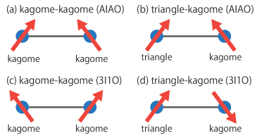
Figure 3: (Color online) Twisted spins of the NN bonds in (a), (b) the AIAO chiral order and (c), (d) the 3I1O chiral order.

We next show the results for typical chiral orders of pyrochlore magnets in the MFA. We summarize the results in Table II.

First, the AF $J_{0}$ and positive $D_{0}$ stabilize the AIAO chiral order. This is because the AIAO chiral order possesses a spin structure in which the total Heisenberg interactions between NN bonds are AF and the spins for all the NN bonds are twisted in the same way, as shown in Figs. 3(a) and 3(b). This chiral order becomes the most stable ground state, for example, at $J_{0}=1$, $D_{0}=0.2$, and $J_{1}=D_{1}=0$. In this chiral order, the spin scalar chirality of three spins in a kagome layer is the same in magnitude as that of a spin in a triangle layer and two spins in a kagome layer, while the signs are opposite.

Second, the FM $J_{0}$ and positive $D_{0}$ stabilize the 2I2O chiral order. In contrast to the AIAO chiral order, this chiral order is not the most stable in our model because the energy reduction of the $J_{0}$ and $D_{0}$ terms is not large.

Third, the combination of the FM $J_{1}$ and negative $D_{1}$ stabilizes the 3I1O chiral order. This is because the 3I1O chiral order possesses the spin structure in which the total Heisenberg interactions between the NN bonds of two spins in a kagome layer are AF and the spins are twisted in the way shown in Fig. 3(c), while the total Heisenberg interactions between the NN bonds of a spin in a triangle layer and a spin in a kagome layer are FM and the spins are twisted in the way shown in Fig. 3(d). (This difference is the key to understanding the kinds of branches of the magnon dispersion, as we will explain in Sect. 3.2.1.) In the 3I1O chiral order, the spin scalar chirality of three spins in a kagome layer are the same in both magnitude and sign as the spin scalar chirality of a spin in a triangle layer and two spins in a kagome layer. This differs from the property of the AIAO and 2I2O chiral orders.

Table 3: Ground-state spin configurations, energies per tetrahedron, and spin scalar chirality in the MFA for the dAIAO and d3I1O chiral magnets. $S_{3}$ is given by $3(S_{3})^{2}=S^{2}=\frac{1}{4}$, and $S_{3}^{\prime}$ and $S^{\prime\prime}_{3}$ are given by $2(S^{\prime}_{3})^{2}+(S^{\prime\prime}_{3})^{2}=S^{2}=\frac{1}{4}$. $\langle\hat{\bm{S}}_{\bm{r}_{2}}\cdot(\hat{\bm{S}}_{\bm{r}_{3}}\times\hat{\bm{S}}_{\bm{r}_{4}})\rangle$ is the spin scalar chirality of three spins in a kagome layer, while $\langle\hat{\bm{S}}_{\bm{r}_{1}}\cdot(\hat{\bm{S}}_{\bm{r}_{2}}\times\hat{\bm{S}}_{\bm{r}_{3}})\rangle$ is the spin scalar chirality of a spin in a triangle layer and two spins in a kagome layer. These chiral magnets satisfy $\langle\hat{\bm{S}}_{\bm{r}_{1}}\cdot(\hat{\bm{S}}_{\bm{r}_{2}}\times\hat{\bm{S}}_{\bm{r}_{3}})\rangle=\langle\hat{\bm{S}}_{\bm{r}_{1}}\cdot(\hat{\bm{S}}_{\bm{r}_{4}}\times\hat{\bm{S}}_{\bm{r}_{2}})\rangle=\langle\hat{\bm{S}}_{\bm{r}_{1}}\cdot(\hat{\bm{S}}_{\bm{r}_{3}}\times\hat{\bm{S}}_{\bm{r}_{4}})\rangle$.

	dAIAO	d3I1O
$\langle\hat{\bm{S}}_{\bm{r}_{1}}\rangle$	${}^{t}(S_{3}\ S_{3}\ S_{3})$	${}^{t}(S_{3}\ S_{3}\ S_{3})$
$\langle\hat{\bm{S}}_{\bm{r}_{2}}\rangle$	${}^{t}(-S_{3}^{\prime}\ -S_{3}^{\prime}\ S_{3}^{\prime\prime})$	${}^{t}(S_{3}^{\prime}\ S_{3}^{\prime}\ -S_{3}^{\prime\prime})$
$\langle\hat{\bm{S}}_{\bm{r}_{3}}\rangle$	${}^{t}(S_{3}^{\prime\prime}\ -S_{3}^{\prime}\ -S_{3}^{\prime})$	${}^{t}(-S_{3}^{\prime\prime}\ S_{3}^{\prime}\ S_{3}^{\prime})$
$\langle\hat{\bm{S}}_{\bm{r}_{4}}\rangle$	${}^{t}(-S_{3}^{\prime}\ S_{3}^{\prime\prime}\ -S_{3}^{\prime})$	${}^{t}(S_{3}^{\prime}\ -S_{3}^{\prime\prime}\ S_{3}^{\prime})$
$\frac{\langle\hat{H}_{\textrm{eff}}\rangle}{N}$	$6(J_{0}+J_{1})S_{3}(S_{3}^{\prime\prime}-2S^{\prime}_{3})$	$6(J_{0}+J_{1})S_{3}(2S^{\prime}_{3}-S_{3}^{\prime\prime})$
	$+6(J_{0}-J_{1})S_{3}^{\prime}(S_{3}^{\prime}-2S^{\prime\prime}_{3})$	$+6(J_{0}-J_{1})S_{3}^{\prime}(S_{3}^{\prime}-2S^{\prime\prime}_{3})$
	$-12(D_{0}+D_{1})S_{3}(S_{3}^{\prime\prime}+S^{\prime}_{3})$	$+12(D_{0}+D_{1})S_{3}(S_{3}^{\prime\prime}+S^{\prime}_{3})$
	$-12(D_{0}-D_{1})S_{3}^{\prime}(S_{3}^{\prime\prime}+S^{\prime}_{3})$	$-12(D_{0}-D_{1})S_{3}^{\prime}(S_{3}^{\prime\prime}+S^{\prime}_{3})$
$\langle\hat{\bm{S}}_{\bm{r}_{2}}\cdot(\hat{\bm{S}}_{\bm{r}_{3}}\times\hat{\bm{S}}_{\bm{r}_{4}})\rangle$	$(S^{\prime}_{3}+S_{3}^{\prime\prime})[S^{\prime\prime}_{3}(S_{3}^{\prime\prime}-S^{\prime}_{3})-2(S_{3}^{\prime})^{2}]$	$-(S^{\prime}_{3}+S^{\prime\prime}_{3})[S^{\prime\prime}_{3}(S^{\prime\prime}_{3}-S^{\prime}_{3})-2(S^{\prime}_{3})^{2}]$
$\langle\hat{\bm{S}}_{\bm{r}_{1}}\cdot(\hat{\bm{S}}_{\bm{r}_{2}}\times\hat{\bm{S}}_{\bm{r}_{3}})\rangle$	$S_{3}(S^{\prime}_{3}+S_{3}^{\prime\prime})^{2}$	$S_{3}(S^{\prime}_{3}+S_{3}^{\prime\prime})^{2}$

Then, there are other chiral orders, whose ground-state energies depend on $J_{0}$, $D_{0}$, $J_{1}$, and $D_{1}$. Their results are summarized in Table III.

First, the dAIAO chiral order is stabilized by the combination of the AF $J_{0}$, the positive $D_{0}$, and the small $J_{1}$ and $D_{1}$. In this chiral order, the directions of the spins in a tetrahedron intersect at a point on the line connecting sublattice 1 and the center of the tetrahedron. Since in the AIAO chiral order the directions of the spins in a tetrahedron intersect at the center of the tetrahedron, the difference between these chiral orders is the displacement of the intersecting point. We can thus regard this as a distorted AIAO chiral order. As we see from Table III, the dAIAO chiral order possesses two properties that are different from the properties of the AIAO chiral order: one is the dependence of the ground-state energy on $J_{1}$ and $D_{1}$; the other is the bond-dependent magnitude of the spin scalar chirality. The former originates from the combination of the stabilization of the AIAO-like spin structure due to $J_{0}$ and $D_{0}$ and the modification of the spin structure due to the corrections of $J_{1}$ and $D_{1}$; the latter originates from the imbalance between the exchange interactions in a kagome layer and those between triangle and kagome layers due to the corrections of $J_{1}$ and $D_{1}$. Actually, we can more clearly understand the origins of the two properties by analyzing the slightly distorted case. In this case, the spin structure in a tetrahedron is determined by choosing $S^{\prime}_{3}$ and $S^{\prime\prime}_{3}$ in the spin structure of the dAIAO chiral order as $S^{\prime}_{3}=S_{3}+\Delta S^{\prime}$ and $S^{\prime\prime}_{3}=S_{3}-2\Delta S^{\prime}$, where $\Delta S^{\prime}$ is a small correction; $\Delta S^{\prime}$ has been chosen because the $S_{3}^{\prime}$ and $S^{\prime\prime}_{3}$ in this choice satisfy the hard-spin constraint within the $O(\Delta S^{\prime})$ terms. By substituting $S^{\prime}_{3}=S_{3}+\Delta S^{\prime}$ and $S^{\prime\prime}_{3}=S_{3}-2\Delta S^{\prime}$ in $\frac{\langle\hat{H}_{\textrm{eff}}\rangle}{N}$, $\langle\hat{\bm{S}}_{\bm{r}_{2}}\cdot(\hat{\bm{S}}_{\bm{r}_{3}}\times\hat{\bm{S}}_{\bm{r}_{4}})\rangle$, and $\langle\hat{\bm{S}}_{\bm{r}_{1}}\cdot(\hat{\bm{S}}_{\bm{r}_{2}}\times\hat{\bm{S}}_{\bm{r}_{3}})\rangle$ of the dAIAO chiral order for Table III and estimating them within the $O(\Delta S^{\prime})$ terms, we obtain

$$\frac{\langle\hat{H}_{\textrm{eff}}\rangle}{N}=(-J_{0}-4D_{0})+4\sqrt{3}(-2J_{1}+D_{1})\Delta S^{\prime},$$ (53)

and

$$\langle\hat{\bm{S}}_{\bm{r}_{2}}\cdot(\hat{\bm{S}}_{\bm{r}_{3}}\times\hat{\bm{S}}_{\bm{r}_{4}})\rangle= -\frac{1}{6\sqrt{3}}-\Delta S^{\prime},$$ (54)

$$\langle\hat{\bm{S}}_{\bm{r}_{1}}\cdot(\hat{\bm{S}}_{\bm{r}_{3}}\times\hat{\bm{S}}_{\bm{r}_{4}})\rangle= \frac{1}{6\sqrt{3}}-\frac{1}{3}\Delta S^{\prime}.$$ (55)

Second, the d3I1O chiral order is stabilized by the combination of the FM $J_{1}$, the negative $D_{1}$, and the corrections of $J_{0}$ and $D_{0}$. We can understand its stabilizing mechanism and properties, which are different from the properties of the 3I1O chiral order, in a similar way as for the dAIAO chiral order. This chiral order can be regarded as a distorted 3I1O chiral order because the difference between it and the 3I1O chiral order is the displacement of the intersection point of the directions of the spins in a tetrahedron. The d3I1O chiral order is stabilized by the combination of the stabilization of a 3I1O-like spin structure due to $J_{1}$ and $D_{1}$ and the modification of the spin structure due to the corrections of $J_{0}$ and $D_{0}$. As a result, its ground-state energy depends on not only $J_{1}$ and $D_{1}$ but also $J_{0}$ and $D_{0}$. Furthermore, there is another property different from the property of the 3I1O chiral order: the bond-dependent magnitude of the spin scalar chirality due to the imbalance between the exchange interactions in a kagome layer and the exchange interactions between triangle and kagome layers. The origins of these two properties can be more clearly understood by analyzing a slightly distorted case of the d3I1O chiral order: we first choose $S^{\prime}_{3}$ and $S^{\prime\prime}_{3}$ in the spin structure of the d3I1O chiral order as $S^{\prime}_{3}=S_{3}+\Delta S^{\prime}$ and $S^{\prime\prime}_{3}=S_{3}-2\Delta S^{\prime}$ with $\Delta S^{\prime}$ because $S_{3}^{\prime}$ and $S_{3}^{\prime\prime}$ satisfy the hard-spin constraint within the $O(\Delta S^{\prime})$ terms; we then estimate the ground-state energy and spin scalar chirality within the $O(\Delta S^{\prime})$ terms as

$$\frac{\langle\hat{H}_{\textrm{eff}}\rangle}{N}=(J_{1}+4D_{1})-4\sqrt{3}(-2J_{0}+D_{0})\Delta S^{\prime},$$ (56)

and

$$\langle\hat{\bm{S}}_{\bm{r}_{2}}\cdot(\hat{\bm{S}}_{\bm{r}_{3}}\times\hat{\bm{S}}_{\bm{r}_{4}})\rangle= \frac{1}{6\sqrt{3}}+\Delta S^{\prime},$$ (57)

$$\langle\hat{\bm{S}}_{\bm{r}_{1}}\cdot(\hat{\bm{S}}_{\bm{r}_{3}}\times\hat{\bm{S}}_{\bm{r}_{4}})\rangle= \frac{1}{6\sqrt{3}}-\frac{1}{3}\Delta S^{\prime}.$$ (58)

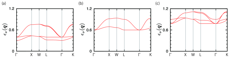
Figure 4: (Color online) Magnon dispersion curves, $\epsilon_{\nu}(\bm{q})$ ($\nu=1,\cdots,4$), in the LSWA for the AIAO chiral magnet at $J_{0}=1$, $J_{1}=D_{1}=0$, and $D_{0}=$ (a) $0.1$, (b) $0.2$, and (c) $0.3$. The symmetrical points are $\Gamma(0\ 0\ 0)$, X$(\pi\ 0\ 0)$, W$(\pi\ \frac{\pi}{2}\ 0)$, L$(\frac{\pi}{2}\ \frac{\pi}{2}\ \frac{\pi}{2})$, and K$(\frac{3\pi}{4}\ \frac{3\pi}{4}\ 0)$.

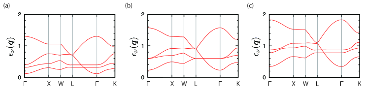
Figure 5: (Color online) Magnon dispersion curves, $\epsilon_{\nu}(\bm{q})$ ($\nu=1,\cdots,4$), in the LSWA for the 3I1O chiral magnet at $J_{1}=-1$, $J_{0}=D_{0}=0$, and $D_{1}=$ (a) $-0.1$, (b) $-0.2$, and (c) $-0.3$.

3.2 Magnon dispersion and specific heat

We turn to the magnon dispersion and specific heat for four chiral magnets in our $S=\frac{1}{2}$ model in the LSWA. The four chiral magnets are the AIAO, 3I1O, dAIAO, and d3I1O chiral magnets; their ordering vectors are all $\bm{Q}=\bm{0}$. We consider these magnets because one of them can be the most stable ground state of our $S=\frac{1}{2}$ model in the MFA, depending on the values of $J_{0}$, $D_{0}$, $J_{1}$, and $D_{1}$. We show the results for the magnon dispersion and specific heat in Sects. 3.2.1 and 3.2.2, respectively.

We obtained the results by numerical calculations. In the numerical calculations, we substituted $N_{x}=N_{y}=N_{z}=128$ in $q_{x}=\pi(\frac{m_{x}}{N_{x}}-\frac{m_{y}}{N_{y}}+\frac{m_{z}}{N_{z}})$, $q_{y}=\pi(\frac{m_{x}}{N_{x}}+\frac{m_{y}}{N_{y}}-\frac{m_{z}}{N_{z}})$, and $q_{z}=\pi(-\frac{m_{x}}{N_{x}}+\frac{m_{y}}{N_{y}}+\frac{m_{z}}{N_{z}})$, with $N_{x}N_{y}N_{z}=N$, $1\leq m_{x}\leq N_{x}$, $1\leq m_{y}\leq N_{y}$, and $1\leq m_{z}\leq N_{z}$; we chose the convergence factor $\Delta$ as $\Delta=10^{-7}$, which is tiny compared with the finite exchange interactions; we chose the values of $J_{0}$, $D_{0}$, $J_{1}$, and $D_{1}$ so as to enable one of the four chiral orders to be most stable at zero temperature in the MFA. For the AIAO chiral magnet, we set $J_{0}=1$, $D_{0}=0.1$, $0.2$, or $0.3$, and $J_{1}=D_{1}=0$. Since the corrections of $J_{1}$ and $D_{1}$ to the AIAO chiral order cause the dAIAO chiral order to be more stable, we set $J_{0}=1$, $D_{0}=0.2$ or $0.3$, $J_{1}=0.5$ or $-0.5$, and $D_{1}=\frac{J_{1}D_{0}}{|J_{0}|}=J_{1}D_{0}$ for the dAIAO chiral magnet. Then, we set $J_{0}=D_{0}=0$, $J_{1}=-1$, and $D_{1}=-0.1$, $-0.2$, or $-0.3$ for the 3I1O chiral magnet. For the d3I1O chiral magnet, we set $J_{0}=-1$, $J_{1}=-1.8$, $D_{0}=0.1$ or $0.2$, and $D_{1}=\frac{J_{1}D_{0}}{|J_{0}|}=J_{1}D_{0}$. Only for the 3I1O chiral magnet, the magnitude of $J_{1}$ is chosen as the energy unit; for the others, the energy unit is the magnitude of $J_{0}$. For each set of the parameters, we numerically calculated the noninteracting magnon dispersion of a chiral magnet using the algorithm explained in Sect. 2.3. We also calculated the specific heat, $C_{v}$, given by

$$C_{v}= \frac{2}{T^{2}}\sum\limits_{\bm{q}}\sum\limits_{\nu=1}^{4}\epsilon_{\nu}(\bm{q})^{2}n[\epsilon_{\nu}(\bm{q})]^{2}\exp[\frac{\epsilon_{\nu}(\bm{q})}{T}],$$ (59)

where $n(\epsilon)$ is the Bose distribution function.

3.2.1 Magnon dispersion

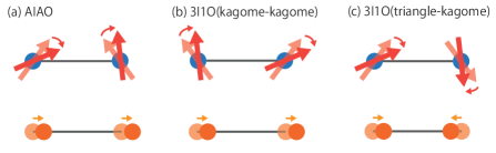
Figure 6: (Color online) Rotations of two spins (upper rows) and the analogous motion of phonons (lower rows) in (a) the AIAO chiral magnet and (b), (c) the 3I1O chiral magnet.

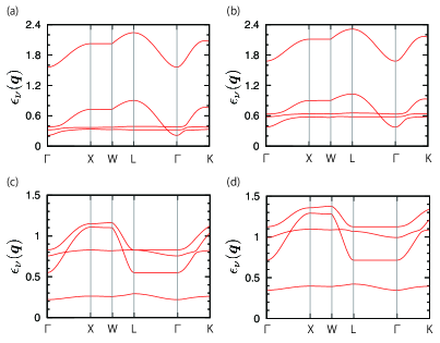
Figure 7: (Color online) Magnon dispersion curves, $\epsilon_{\nu}(\bm{q})$ ($\nu=1,\cdots,4$), in the LSWA for the dAIAO chiral magnet at $J_{0}=1$, $D_{1}=J_{1}D_{0}$, and $(J_{1},D_{0})=$ (a) $(0.5,0.2)$, (b) $(0.5,0.3)$, (c) $(-0.5,0.2)$, and (d) $(-0.5,0.3)$.

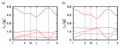
Figure 8: (Color online) Magnon dispersion curves, $\epsilon_{\nu}(\bm{q})$ ($\nu=1,\cdots,4$), in the LSWA for the d3I1O chiral magnet at $J_{0}=-1$, $J_{1}=-1.8$, $D_{1}=J_{1}D_{0}$, and $D_{0}=$ (a) $0.2$, and (b) $0.3$.

Before giving the results for the magnon dispersions, we define a quasiacoustic or an optical branch and explain the appropriateness of the definitions. A quasiacoustic branch is defined as a branch that increases with increasing displacement from $\bm{q}=\bm{Q}$, while an optical branch is defined as a branch that decreases. In other words, the quasiacoustic and optical branches are respectively defined as convex and concave functions of $\bm{q}$ around $\bm{q}=\bm{Q}$. (The convex or concave function means that the energy at $\bm{q}=\bm{Q}$ is smallest or largest, respectively, in momenta near $\bm{q}=\bm{Q}$.) We do not impose any conditions on the value at $\bm{q}=\bm{Q}$ or the power of the $\bm{q}$ dependence. This is because the above definitions are appropriate for distinguishing whether the mode of a branch is acoustic type or optical type. The acoustic type mode corresponds to the same-phase motion, while the optical type mode corresponds to the $180^{\circ}$-out-of-phase motion [17]. Since the same-phase and $180^{\circ}$-out-of-phase motion have the lowest and largest energies, respectively, for $\bm{q}=\bm{Q}$, the above definitions are appropriate. We use the quasiacoustic mode rather than the acoustic mode because the acoustic mode in the exact sense appears only in a few cases, such as antiferromagnets.

We start with the magnon dispersion of the AIAO chiral magnet. We can see its three properties from Fig. 4. First, a gap is opened at the $\Gamma$ point. (This gap is not due to the finite convergence factor $\Delta=10^{-7}$ because $\Delta$ is much smaller than the value of the gap; as we will see below, the situation is the same even in the other three chiral magnets.) Since this gap increases as a function of $D_{0}$ and is not equal to the value of $D_{0}$, this gap is induced by the combination of $D_{0}$ and $J_{0}$. This property is distinct from the magnon dispersion of a nonchiral magnet because a commensurate nonchiral magnet has gapless excitation at $\bm{q}=\bm{0}$. Second, the magnon energies at the $\Gamma$ point are partially or completely degenerate: the degeneracy is fourfold at $D_{0}=0.2$ and threefold at $D_{0}=0.1$ and $0.3$. The partial lifting of the degeneracy arises from the DM interaction because the difference between the nondegenerate energies at the $\Gamma$ point is approximately equal to $D_{0}-0.2$. Third, all the branches are quasiacoustic near the $\Gamma$ point. This is similar for a nonchiral magnet.

Figure 5 shows three properties of the magnon dispersion of the 3I1O chiral magnet. First, a gap is opened at the $\Gamma$ point in a similar way to that for the AIAO chiral magnet. This gap is mainly induced by $D_{1}$ because the value of this gap approximately corresponds to the magnitude of $D_{1}$. Second, the magnon energies at the $\Gamma$ point are degenerate only at $D_{1}=-0.2$, while at $D_{1}=-0.1$ and $-0.3$ the degeneracy is completely lifted. The lifting of the twofold degeneracy arises from $D_{1}$ because the difference between the second and third lowest energy branches at the $\Gamma$ point is approximately equal to $|D_{1}+0.2|$. Third, the highest-energy branch is optical near the $\Gamma$ point, while the other three branches are quasiacoustic. The appearance of the optical branch is distinct from the property of not only a nonchiral magnet with $\bm{Q}=\bm{0}$ but also the AIAO chiral magnet.

By a similar analysis for phonons, we can understand why all the branches near $\bm{q}=\bm{0}$ are quasiacoustic in the AIAO chiral magnet, while an optical branch appears in the 3I1O chiral magnet. Let us begin by recalling the mechanism of the acoustic and optical branches for phonons [17]. For this purpose, we consider an one-dimensional lattice of two different ions; the two different ions result in a unit cell with a two-sublattice structure. In this case, the phonon dispersion has an acoustic branch and an optical branch. The acoustic branch arises from the same-phase displacement of two different ions in each unit cell from the equilibrium positions, while the optical branch arises from the $180^{\circ}$-out-of-phase displacement. Namely, if we understand how fluctuations modify the ground-state configuration determined in a classical or semiclassical theory, we can understand whether a branch of the dispersion of bosonic quasiparticles is quasiacoustic or optical. Thus, in a similar way to phonons, we can understand the mechanism of the quasiacoustic and optical branches for magnons. We first consider the AIAO chiral magnet. Figure 6(a) shows the relative configuration of two spins for two of the four sublattices for the AIAO chiral magnet. If the fluctuations cause a clockwise rotation of the left-hand-side spin in Fig. 6(a), the right-hand-side spin rotates as the same-phase rotation. Since the relative configurations of two spins are the same for any pair of the four sublattices, all the branches for the AIAO chiral magnet are quasiacoustic. Similarly, we can understand the type of branches for the 3I1O chiral magnet. As we see from Figs. 6(b) and 6(c), there are two types of relative configurations of two spins for two of the four sublattices for the 3I1O chiral magnet: one is for two of sublattices 2, 3, and 4, while the other is for sublattice 1 and sublattice 2, 3, or 4. In the former configuration, the fluctuations induce the same-phase rotations of the two spins [Fig. 6(b)], while in the latter configuration, the $180^{\circ}$-out-of-phase rotations are induced [Fig. 6(c)]. Thus, the same-phase rotations for two of sublattices 2, 3, and 4 lead to three quasiacoustic branches of the magnon dispersion, and the $180^{\circ}$-out-of-phase rotations for sublattice 1 and sublattice 2, 3, or 4 lead to one optical branch.

Then, from Figs. 7(a)–7(d), we can find three properties of the magnon dispersion of the dAIAO chiral magnet. First, a gap is opened at the $\Gamma$ point in a similar way to that for the AIAO chiral magnet. Second, in contrast to the AIAO chiral magnet, there is no degeneracy of the magnon energies at the $\Gamma$ point. Third, the branches near the $\Gamma$ point are all quasiacoustic. This is the same as the property for the AIAO chiral magnet. We can understand its mechanism in a similar way to that for the AIAO chiral magnet because the main difference between these chiral magnets is the modification of the directions of the spins at sublattices 2, 3, and 4 (see Sect. 3.1). Thus, except the absence of the degeneracy, the magnon dispersion of the dAIAO chiral magnet is similar to that of the AIAO chiral magnet.

We can also find similarities and differences between the 3I1O and d3I1O chiral magnets by comparing Figs. 5 and 8. The main similarities are the gap of the lowest-energy branch at the $\Gamma$ point and the numbers of quasiacoustic and optical branches near the $\Gamma$ point; the main difference is the degeneracy of the magnon energies at the $\Gamma$ point. However, whether the degeneracy is present or absent depends on the value of $\frac{D_{1}}{J_{1}}$ (see Fig. 5). Thus, the magnon dispersion curves of the 3I1O and d3I1O chiral magnets are similar.

3.2.2 Specific heat

We turn to the results for the specific heat of the AIAO chiral magnet. (Since we use the LSWA, which may be appropriate only for low temperature, we focus on the results at low temperature.) The results are shown in Figs. 9 and 10(a). We can find three properties. First, the specific heat decreases as $D_{0}$ increases. This is because the dominant contributions to the specific heat are from the low-energy magnons, and because the increase in $D_{0}$ causes the increase in the lowest-energy branch at the $\Gamma$ point [see Figs. 4(a)–4(c)]. Second, it is difficult to uniquely determine the power of the temperature dependence of the specific heat in the low-temperature region. (The region of $0\leq T\leq 0.3$ can be regarded as a low-temperature region because the typical magnitude of $J_{0}$ is approximately $30$ meV–$30$ K, and $T=0.3=0.3J_{0}$ corresponds to $T=0.3$–$10$ K.) The difficulty may arise from the combination of the gap in the lowest-energy magnon branch at the $\Gamma$ point and the complex dispersion curves. Third, the ratio of $C_{v}$ to $T$ has a peak at a low temperature due to the absence of gapless excitation.

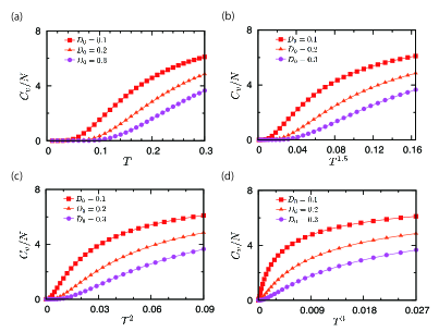
Figure 9: (Color online) Low-temperature $\frac{C_{v}}{N}$ in the LSWA for the AIAO chiral magnet as a function of (a) $T$, (b) $T^{1.5}$, (c) $T^{2}$, and (d) $T^{3}$; $J_{0}$, $D_{0}$, $J_{1}$, and $D_{1}$ are chosen as $J_{0}=1$, $J_{1}=D_{1}=0$, and $D_{0}=0.1$, $0.2$, or $0.3$.

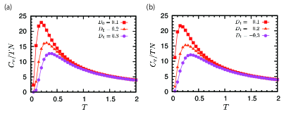
Figure 10: (Color online) Low-temperature $\frac{C_{v}}{NT}$ in the LSWA for (a) the AIAO chiral magnet and (b) the 3I1O chiral magnet.

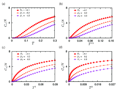
Figure 11: (Color online) Low-temperature $\frac{C_{v}}{N}$ in the LSWA for the 3I1O chiral magnet as a function of (a) $T$, (b) $T^{1.5}$, (c) $T^{2}$, and (d) $T^{3}$; $J_{0}$, $D_{0}$, $J_{1}$, and $D_{1}$ are chosen as $J_{1}=-1$, $J_{0}=D_{0}=0$, and $D_{1}=-0.1$, $-0.2$, or $-0.3$.

The other three chiral magnets also have the same three properties of the specific heat as those of the AIAO chiral magnet. The results for the 3I1O chiral magnet are shown in Figs. 11 and 10(b), while the results for the other chiral magnets are not shown. Then, we can understand the origin of each property in the same way as for the AIAO chiral magnet because the optical branch near the $\Gamma$ point and the degeneracy of the magnon energies do not qualitatively change the specific heat.

4 Discussion

We first argue the applicability of the LSWA. In the LSWA, we express the low-energy effective Hamiltonian of a magnetically ordered insulator in terms of the quadratic terms of the magnon operators, as explained in Sect. 2.3. For the arguments about the applicability, we need to discuss the effects of the terms neglected in the LSWA. The neglected terms can be classified into three parts. One part consists of the zeroth-order terms of the magnon operators. Since the zeroth-order terms do not usually change the most stable state of a three-dimensional magnet, their effects will be quantitative. Another part consists of the fourth-order and higher-order terms. The order of the fourth-order terms is higher than that of the terms considered in the LSWA by a factor of $\frac{\hat{b}_{ml}^{\dagger}\hat{b}_{ml}}{2S}$. Since the factor is small for large $S$ or a low temperature or both, the effects of the fourth-order and higher-order terms are negligible at low temperatures even for $S=\frac{1}{2}$; a low temperature is necessary because at low temperatures the number of excited magnons is small. Actually, this has been demonstrated for an $S=\frac{1}{2}$ collinear antiferromagnet on a square lattice [18]. Since the effects tend to be smaller in a three-dimensional system than in a two-dimensional system, the fourth-order and higher-order terms also will not change our main results qualitatively. The other part consists of the third-order terms. The third-order terms are characteristic of noncollinear magnets [19], such as a coplanar antiferromagnet and chiral magnets. In contrast to the fourth-order and higher-order terms, the third-order terms can affect the magnon properties even at low temperatures. However, we believe that our main results remain qualitatively unchanged even if the third-order terms are taken into account. This can be understood as follows. First of all, the third-order terms, such as $\hat{b}^{\dagger}_{ml}\hat{b}^{\dagger}_{nl^{\prime}}\hat{b}_{nl^{\prime}}$, connect the ground state to the lowest excited state. This suggests that the effects of the third-order terms are small for a large energy difference between these states and large for a small energy difference. In addition, the energy difference becomes large or small in the absence or presence of frustration, respectively. Since the frustration of the Heisenberg interactions is removed in the chiral magnets considered in this paper, the effects of the third-order terms may be small. Actually, the energy difference for the AIAO chiral magnet is $\Delta E=E_{\textrm{ex}}-E_{\textrm{gs}}=2(J_{1}+4D_{1})-2(-J_{0}-4D_{0})=2J_{0}+8D_{0}$, which is large with our parameters (e.g., $\Delta E=3.6$ for $J_{0}=1$, $D_{0}=0.2$ and $J_{1}=D_{1}=0$); $E_{\textrm{ex}}$ and $E_{\textrm{gs}}$ are the energies of the lowest excited and ground states, respectively. Here the lowest excited state for the AIAO chiral magnet is obtained by replacing the AIAO spin structures of two of $N$ tetrahedra by the 3I1O ones because the lowest-energy excitation corresponds to the spin flip at the center in Fig. 2(a). Similarly, we obtain the large energy difference for the 3I1O chiral magnet, $\Delta E=E_{\textrm{ex}}-E_{\textrm{gs}}=2(-J_{0}-4D_{0})-2(J_{1}+4D_{1})=2|J_{1}|+8|D_{1}|$ (e.g., $\Delta E=3.6$ for $J_{1}=-1$, $D_{1}=-0.2$, and $J_{0}=D_{0}=0$); the lowest excited state is obtained by replacing the 3I1O/1I3O spin structures of two of $N$ tetrahedra by the AIAO ones; this replacement corresponds to the spin flip at the center in Fig. 2(b).

We next compare our results with those of several experiments. The results for the AIAO or dAIAO chiral magnet are compared with experimental results for the AIAO type chiral magnet, and the results for the 3I1O or d3I1O chiral magnet are compared with experimental results for the 3I1O type chiral magnet. This is because it is difficult to distinguish between the AIAO and dAIAO chiral magnets and between the 3I1O and d3I1O chiral magnets in terms of the magnon dispersion and specific heat, as shown in Sect. 3.2. Our results for the AIAO or dAIAO chiral magnet are consistent with the experimental results for the AIAO type chiral magnet in Sm₂Ir₂O₇ and Nd₂Ir₂O₇: the gap at the $\Gamma$ point is consistent with the absence of the Goldstone type gapless excitation in a neutron scattering measurement on Sm₂Ir₂O₇ [9]; the peak of $C_{v}/T$ is consistent with the peak observed experimentally for Nd₂Ir₂O₇ [20]. We believe this comparison is meaningful, although Sm₂Ir₂O₇ and Nd₂Ir₂O₇ may have the strong SOC and the low-energy effective model may include the exchange interactions neglected in our model. This is because both models include the relevant exchange interactions for the AIAO type chiral magnet, and because the effects of the neglected interactions may be some quantitative modifications. Then, owing to a lack of experiments on the magnon dispersion in the 3I1O type chiral magnet, we cannot compare the results for the 3I1O or d3I1O chiral magnets with the experimental results. In addition, our results for the specific heat are not comparable to the experimental results in the 3I1O type chiral magnet for Dy₂Ti₂O₇ [21, 22]. This is because an external magnetic field is absent in our case but present in the experiments [21, 22], and because the Zeeman splitting due to the external magnetic field causes a Schottky type peak of the specific heat as a function of temperature.

For future experiments, we propose that if we measure the magnon dispersion of the 3I1O type chiral magnet, we will observe the gap at the $\Gamma$ point and the optical branch near the $\Gamma$ point. These observations may hold even in the presence of an external magnetic field as long as the 3I1O type chiral order is the most stable. Thus, by comparing the experimental result with our result, we can identify the 3I1O type chiral order.

5 Summary

We have studied the magnon dispersion and specific heat in four chiral magnets with $\bm{Q}=\bm{0}$ at low temperatures using the LSWA for the effective model of the $S=\frac{1}{2}$ pyrochlore oxides. We have shown that the optical branch of the magnon dispersion near $\bm{Q}=\bm{0}$ emerges only in the 3I1O and d3I1O chiral magnets, while the branches are all quasiacoustic in the AIAO and dAIAO chiral magnets. This is an experimentally distinguishable difference between 3I1O type and AIAO type chiral magnets and useful for experimentally identifying these chiral orders. Also, we have shown the gap of the magnon dispersion at $\bm{q}=\bm{0}$ in all the chiral magnets, indicating the absence of the Goldstone type gapless excitation. This is distinct from the property for a nonchiral magnet and a characteristic of chiral magnets. Then, we have shown that the specific heat has no qualitative difference among the four magnets. It is thus difficult to determine the kinds of chiral orders from the specific heat.

Appendix A Derivation of Eq. (43)

We can derive Eq. (43) using the Holstein-Primakoff transformation. In the Holstein-Primakoff transformation, the spin operators are expressed in terms of creation and annihilation operators of a magnon as follows:

$$\hat{S}^{\prime z}_{ml}=S-\hat{b}_{ml}^{\dagger}\hat{b}_{ml},$$ (60)

$$\hat{S}^{\prime+}_{ml}=\sqrt{2S-\hat{b}_{ml}^{\dagger}\hat{b}_{ml}}\hat{b}_{ml},$$ (61)

$$\hat{S}^{\prime-}_{ml}=\hat{b}_{ml}^{\dagger}\sqrt{2S-\hat{b}_{ml}^{\dagger}\hat{b}_{ml}}.$$ (62)

Equations (61) and (62) can be expanded as follows in terms of series of $\hat{b}_{ml}^{\dagger}\hat{b}_{ml}/2S$:

$$\hat{S}^{\prime+}_{ml}= \sqrt{2S}\Bigl{(}1-\frac{\hat{b}_{ml}^{\dagger}\hat{b}_{ml}}{2S}\Bigr{)}^{\frac{1}{2}}\hat{b}_{ml},$$ (63)

$$\hat{S}^{\prime-}_{ml}= \hat{b}_{ml}^{\dagger}\sqrt{2S}\Bigl{(}1-\frac{\hat{b}_{ml}^{\dagger}\hat{b}_{ml}}{2S}\Bigr{)}^{\frac{1}{2}}.$$ (64)

In the LSWA, we can approximate Eqs. (63) and (64) as the first-order terms of the magnon operator because the LSWA includes terms up to the second order in the Hamiltonian. Namely, Eqs. (63) and (64) are approximated as $\hat{S}^{\prime+}_{ml}=\sqrt{2S}\hat{b}_{ml}$ and $\hat{S}^{\prime-}_{ml}=\hat{b}_{ml}^{\dagger}\sqrt{2S}$. Thus, $\hat{S}^{\prime x}_{ml}$ and $\hat{S}^{\prime y}_{ml}$ are given by

$$\hat{S}^{\prime x}_{ml}=\sqrt{\frac{S}{2}}(\hat{b}_{ml}+\hat{b}_{ml}^{\dagger}),$$ (65)

$$\hat{S}^{\prime y}_{ml}=-i\sqrt{\frac{S}{2}}(\hat{b}_{ml}-\hat{b}_{ml}^{\dagger}).$$ (66)

By using Eqs. (60), (65), and (66), we can express Eq. (38) in terms of the magnon operators. Then, using their Fourier coefficients (e.g., $\hat{b}_{\bm{q}l}=\frac{1}{\sqrt{N}}\sum\limits_{m}e^{i\bm{q}\cdot(\bm{R}_{m}+\bm{r}_{l})}\hat{b}_{ml}$), we can express Eq. (38) as the sum of the zero-order term and second-order terms of the magnon operators in the LSWA; the zero-order term is given by $NS(S+1)\sum_{l,l^{\prime}}M_{ll^{\prime}}^{\prime zz}(\bm{0})$ and the second-order terms are given by Eq. (43).

References

• [1] F. Bloch, Z. Phys. 61, 206 (1930).
• [2] J. C. Slater, Phys. Rev. 35, 509 (1930).
• [3] T. Holstein and H. Primakoff, Phys. Rev. 58, 1098 (1940).
• [4] F. Dyson, Phys. Rev. 102, 1217 (1956).
• [5] F. Dyson, Phys. Rev. 102, 1230 (1956).
• [6] K. Yosida, Theory of Magnetism (Springer Science & Business Media, New York, 1996).
• [7] J. Kanamori, Magnetism (Shokabo, Japan, 1969).
• [8] J. S. Gardner, M. J. P. Gingras and J. E. Greedan, Rev. Mod. Phys. 82, 53 (2010).
• [9] C. Donnerer, M. C. Rahn, M. M. Sala, J. G. Vale, D. Pincini, J. Strempfer, M. Krisch, D. Prabhakaran, A. T. Boothroyd, and D. F. McMorrow, Phys. Rev. Lett. 117, 037201 (2016).
• [10] C. Castelnovo, R. Moessner and S. L. Sondhi, Nature 451, 42 (2008).
• [11] A. G. Del Maestro and M. J. P. Gingras, J. Phys.: Condens. Matter 16, 3339 (2004).
• [12] S. Toth and B. Lake, J. Phys.: Condens. Matter 27, 166002 (2015).
• [13] N. Arakawa, Phys. Rev. B 94, 155139 (2016).
• [14] T. Moriya, Phys. Rev. 120, 91 (1960).
• [15] M. Elhajal, B. Canals, R. Sunyer, and C. Lacroix, Phys. Rev. B 71, 094420 (2005).
• [16] J. Colpa, Physica A 93, 327 (1978).
• [17] N. W. Ashcroft and N. D. Mermin, Solid State Physics (Thomson Learning, Inc., New York, 1976).
• [18] A. W. Sandvik, Phys. Rev. B 56, 11678 (1997), and references therein.
• [19] M. E. Zhitomirsky and A. L. Chernyshev, Rev. Mod. Phys. 85, 219 (2013).
• [20] K. Matsuhira, M. Wakeshima, Y. Hinatsu, and S. Takagi, J. Phys. Soc. Jpn. 80, 094701 (2011).
• [21] A. P. Ramirez, A. Hayashi, R. J. Cava, R. Siddharthan, and B. S. Shastry, Nature 399, 333 (1999).
• [22] D. J. Morris, D. A. Tennant, S. A. Grigera, B. Klemke, C. Castelnovo, R. Moessner, C. Czternasty, M. Meissner, K. C. Rule, J.-U. Hoffmann, K. Kiefer, S. Gerischer, D. Slobinsky, and R. S. Perry, Science 326, 411 (2009).