A matrix formulation of the Tau method for the numerical solution of non-linear problems

Abstract

The purpose of this research is to propose a new approach named the shifted Bessel Tau (SBT) method for solving higher-order ordinary differential equations (ODE). The operational matrices of derivative, integral and product of shifted Bessel polynomials on the interval $[a,b]$ are calculated. These matrices together with the Tau method are utilized to reduce the solution of the higher-order ODE to the solution of a system of algebraic equations with unknown Bessel coefficients. The comparisons between the results of the present work and other the numerical method are shown that the present work is computationally simple and highly accurate.

1 Introduction

Differential equations and their solutions play a major role in science and engineering. A physical event can be modeled by the differential equation, an integral equation or an integro-differential equation or a system of these equations. Since few of these equations cannot be solved explicitly, it is often necessary to resort to the numerical techniques which are appropriate combinations of numerical integration and interpolation. The solution of this equation occurring in physics, biology and engineering are based on numerical methods. One of the powerful method for solving the ordinary differential equations, integral and integro-differential equations are spectral methods in both terms of accuracy and simplicity. Spectral methods, in the context of numerical schemes for differential equations, generically belong to the family of weighted residual methods (WRMs) refIntroduction01 . WRMs represent a particular group of approximation techniques, in which the residuals (or errors) are minimized in a certain way and thereby leading to specific methods, including Galerkin, Petrov-Galerkin, collocation and Tau formulations refIntroduction02 ; refIntroduction03 ; refIntroduction04 ; refIntroduction05 . The basis of spectral method is always polynomials (orthogonal polynomials). These types of basis for approximation of enough smooth functions in the finite domain leads to the exponential convergence.
 In Tau method, the operational matrices of derivative, integral and product of basis functions are obtained and then these matrices together to reduce the solution of these problems to the solution of a system of algebraic equations. Tau method is based on expanding the required approximate solution as the elements of a complete set of basis functions. Polynomial series and orthogonal functions have received considerable attention in dealing with various problems of differential, integral and integro-differential equations. Polynomials are incredibly useful mathematical tools as they are simply defined and can be calculated quickly on computer systems and represent a tremendous variety of functions. They can be differentiated and integrated easily, and can be pieced together to form spline curves that can approximate any function to any accuracy desired. Also, the main characteristic of this technique is that it reduces these problems to those of solving a system of algebraic equations, thus greatly simplifies the problems.
In recent years, the differential, integral and integro-differential equations have been solved using the homotopy perturbation method refIntroduction12 ; refIntroduction13 , the fractional order of rational Bessel functions collocation (FRBC) method Parand.Ghaderi.Electonical , the radial basis functions method refIntroduction14 , the collocation method refIntroduction15 , the Homotopy analysis method refIntroduction16 ; refIntroduction17 , the Tau method refIntroduction18 ; refIntroduction19 , the Variational iteration method refIntroduction20 ; refIntroduction21 , the Legendre matrix method refIntroduction10 ; refIntroduction22 , the Haar Wavelets operational matrix refIntroduction23 , the Shifted Chebyshev direct method refIntroduction24 , the generalized fractional order of the Chebyshev collocation approach refIntroduction42 , the Legendre Wavelets operational matrix refIntroduction25 , Sine-Cosine Wavelets operational matrix refIntroduction26 , the operational matrices of Bernstein polynomials refIntroduction27 . Razzaghi et al. in refIntroduction28 ; refIntroduction29 ; refIntroduction30 presented the integral and product operational matrices based on the Fourier, the Taylor and the shifted-Jacobi series. Parand et al. in refIntroduction30_1 ; refIntroduction30_2 ; Parand.Ghaderi.European ; Parand.Ghaderi.SeMA applied the spectral method to solve nonlinear ordinary differential equations on semi-infinite intervals. Their approach was based on a rational Tau method. They obtained the operational matrices of derivative and product of rational Chebyshev and Legendre functions and then applied these matrices together with the Tau method to reduce the solution of these problems to the solution of a system of algebraic equations. Doha refIntroduction31 has derived the shifted Jacobi operational matrix of fractional derivatives which is applied together with the spectral Tau method for the numerical solution of dynamical systems.Yousefi et al. in refIntroduction32 ; refIntroduction33 ; refIntroduction34 ; refIntroduction35 have presented Legendre wavelets and Bernstein operational matrices and used them to solve miscellaneous systems. Also, recently, in refIntroduction36 a new shifted-Chebyshev operational matrix of fractional integration of arbitrary order is introduced and applied together with the spectral Tau method for solving linear fractional differential equations (FDEs). In refIntroduction37 ; refIntroduction38 the operational matrix form in a Hybrid of block-pulse functions and another set of functions like Taylor series, Legendre and Chebyshev has been used for finding the solution of the various classes of dynamical systems. Lakestani refIntroduction39 constructed the operational matrix of fractional derivative of order $\alpha$ in the Caputo sense using the linear B-spline functions. In refIntroduction40 , a general formulation for the d dimensional orthogonal functions and their derivative and product matrices has been presented. Ordinary operational matrices have been utilized together with the Tau method to reduce the solution of partial differential equations (PDEs) to the solution of a system of algebraic equations. Recently in refIntroduction41 , a class of two dimensional nonlinear Volterra’s integral equations has been solved using operational matrices of Legendre polynomials. The operational matrices of integration and product together with the collocation points have been utilized to reduce the solution of the integral equation to the solution of a nonlinear algebraic equation system.

The remainder of the paper is organized as follows: In section 2, the function approximation and convergence of the method by using Bessel polynomials are illustrated . In sections 3, the general procedure for formulation of operational matrices of integration, differentiation, and product are explained and are proved. In section 4, our numerical findings and demonstrate the validity, accuracy and applicability of the operational matrices by considering numerical examples are reported. Also a conclusion is given in the last section.

2 Bessel Polynomials

The Bessel functions arise in many problems in physics possessing cylindrical symmetry, such as the vibrations of circular drumheads and the radial modes in optical fibers. Bessel functions are usually defined as a particular solution of a linear differential equation of the second order which known as Bessel’s equation.

Bessel differential equation of order $n\in\mathbb{R}$ is:

$$x^{2}\frac{d^{2}y(x)}{dx^{2}}+x\frac{dy(x)}{dx}+(x^{2}-n^{2})y(x)=0,~{}~{}x\in(-\infty,\infty).$$ (1)

One of the solutions of Eq. (1) by applying the method of Frobenius is as follows refBesselPol03 :

$$J_{n}(x)=\sum_{r=0}^{\infty}\frac{(-1)^{r}}{r!(n+r)!}(\frac{x}{2})^{2r+n},$$ (2)

where series (2) is convergent for all $x\in(-\infty,\infty)$.

Bessel functions and polynomials are used to solve the more number of problems in physics, engineering, mathematics, and etc., such as Blasius equation, Lane-Emden equations, integro-differential equations of the fractional order, unsteady gas equation, systems of linear Volterra integral equations, high-order linear complex differential equations in circular domains, systems of high-order linear Fredholm integro-differential equations, nolinear Thomas-Fermi on semi-infinite domain, etc. refBesselPol04 ; refBesselPol05 ; refBesselPol09 ; refBesselPol10 ; refBesselPol11 ; refBesselPol12 ; refBesselPol13 ; refBesselPol14 ; refBesselPol15 ; refBesselPol16 ; Parand.Ghaderi.Electonical .

Bessel polynomials has been introduced as follows refBesselPol12 :

$$B_{n}(x)=\sum_{r=0}^{[\frac{N-n}{2}]}\frac{(-1)^{r}}{r!(n+r)!}(\frac{x}{2})^{2r+n},~{}~{}x\in[0,1].$$

where $n\in\mathbb{N}$, and $N$ is the number of basis of Bessel polynomials.
Now, We introduce new shifted Bessel equation in the interval $[a,b]$ by:

$$Q_{n}(x)=B_{n}(\frac{x-a}{b-a}),~{}~{}x\in[a,b],~{}~{}n=0,1,2,...,N.$$

where $a,b\in\mathbb{R}$.

2.1 Approximation of functions

Let us define $\Gamma=\{x|~{}a\leq x\leq b\}$ and
$L^{2}_{w}(\Gamma)=\{~{}v:\Gamma\rightarrow\mathbb{R}|v$ is measurable and $\parallel v\parallel_{w}<\infty\}$, where

$$\parallel v\parallel_{w}=\left(\int^{b}_{a}|v(x)|^{2}w(x)dx\right)^{1/2},$$

with $w(x)=\frac{1}{b-a}$, is the norm induced by inner product of the space $L^{2}_{w}(\Gamma)$ as follows:

$$\langle v,u\rangle_{w}=\int^{b}_{a}{v(x)u(x)w(x)}dx.$$

Now, suppose that

$$\mathfrak{Q}_{N}=~{}span\{Q_{0}(x),Q_{1}(x),\dots,Q_{N}(x)\},$$

where $\mathfrak{Q}_{N}$ is a finite-dimensional subspace of $L^{2}_{w}(\Gamma)$, dim ($\mathfrak{Q}_{N})=N+1$, so $\mathfrak{Q}_{N}$ is a closed subspace of $L_{w}^{2}(\Gamma)$. Therefore, $\mathfrak{Q}_{N}$ is a complete subspace of $L_{w}^{2}(\Gamma)$. Assume that $f(x)$ be an arbitrary element in $L_{w}^{2}(\Gamma)$. Thus $f(x)$ has a unique best approximation in $\mathfrak{Q}_{N}$ subspace, say $\hat{b}\in\mathfrak{Q}_{N}$, that is

$$\exists~{}\hat{b(x)}\in\mathfrak{Q}_{N},~{}~{}~{}\forall~{}b(x)\in\mathfrak{Q}_{N},~{}~{}\parallel f(x)-\hat{b(x)}\parallel_{w}\leq\parallel f(x)-b(x)\parallel_{w}.$$

Notice that we can write $b(x)$ function as a linear combination of the basis vectors of $\mathfrak{Q}_{N}$ subspace.

We know function of $f(x)$ can be expanded by $N+1$ terms of Bessel polynomials as:

$$f(x)=f_{N}(x)+R(x),$$

that is

$$f_{N}=\sum^{N}_{n=0}{a_{n}Q_{n}(x)}=A^{T}Q(x),$$ (3)

where $Q(x)=[Q_{0}(x),Q_{1}(x),\cdots,Q_{N}(x)]^{T}$ and $R(x)\in\mathfrak{Q}^{\perp}_{N}$ that ${\mathfrak{Q}}^{\perp}_{N}$ is the orthogonal complement. So $f(x)-f_{N}(x)\in\mathfrak{Q}_{N}^{\perp}$ and $b(x)\in\mathfrak{Q}_{N}$ are orthogonal which we denote it by:

$$\big{(}f(x)-f_{N}(x)\big{)}\perp b(x),$$

thus $f(x)-f_{N}(x)$ vector is orthogonal over all of basis vectors of $\mathfrak{Q}_{N}$ subspace as:

$$\langle f(x)-f_{N}(x),Q_{i}(x)\rangle_{w}=\langle f(x)-A^{T}Q(x),Q_{i}(x)\rangle_{w}=0,~{}i=0,1,\cdots,N,$$

hence

$$\langle f(x)-A^{T}Q(x),Q^{T}(x)\rangle_{w}=0,$$

therefore A can be obtained by

$$\langle f(x),Q^{T}(x)\rangle_{w}=\langle A^{T}Q(x),Q^{T}(x)\rangle_{w},$$

$$A^{T}=\langle f(x),Q^{T}(x)\rangle_{w}\langle Q(x),Q^{T}(x)\rangle_{w}^{-1},$$

where

$$K=\langle Q(x),Q^{T}(x)\rangle_{w}=\int_{a}^{b}{Q(x)Q(x)^{T}}w(x)dx,$$ (4)

is an $(N+1)\texttimes(N+1)$ matrix and is said dual matrix of $Q(x)$.

2.2 Convergence of the method

The following theorem shows that by increasing $N$, the approximation solution $f_{N}(x)$ is convergent to $f(x)$ exponentially.

Theorem 1. (Taylor’s formula) Suppose that $f(x)\in C[0,b]$ and $D^{k}f(x)\in C[0,b]$, where $k=0,1,...,N$. Then we have

$$f(x)=\sum_{i=0}^{N}\frac{x^{i}}{i!}D^{i}f(0^{+})+\frac{x^{N+1}}{(N+1)!}D^{N+1}f(\xi),$$ (5)

with $0\leqslant\xi\leqslant x,~{}\forall x\in[0,b]$. And thus

$$|f(x)-\sum_{i=0}^{N}\frac{x^{i}}{i!}D^{i}f(0^{+})|\leqslant M\frac{x^{N+1}}{(N+1)!},$$ (6)

where $M\geqslant|D^{N+1}f(\xi)|$.
Proof: See Ref. Odibat.Momani .

Theorem 2 Suppose that $D^{k}f(x)\in C[0,b]$ for $k=0,1,...,N,$ and $\mathfrak{Q}_{N}$ is the subspace generated by $\{Q_{0}(x),~{}Q_{1}(x),...,~{}Q_{N}(x)\}$. If $f_{N}(x)=F^{T}Q(x)$ is the best approximation to $f$ from $\mathfrak{Q}_{N}$ , then the error bound is presented as follows

$$\parallel f(x)-f_{N}(x)\parallel_{w}\leqslant\frac{M}{(N+1)!}\big{(}\frac{b^{2N+2}}{(2N+3)}\big{)}^{\frac{1}{2}},$$ (7)

where $M\geqslant|D^{N+1}f(x)|,~{}~{}x\in[0,b].$
Proof. By theorem 1, we have $y(x)=\sum_{i=0}^{N}\frac{x^{i}}{i!}D^{i}f(0^{+})$ and

$$|f(x)-y(x)|\leqslant M\frac{x^{N+1}}{N+1!}.$$

Since the best approximation to $f(x)$ from $\mathfrak{Q}_{N}$ is $F^{T}Q(x)$, and $y(x)\in\mathfrak{Q}_{N}$, thus

$$\parallel f(x)-f_{N}(x)\parallel_{w}^{2}\leqslant\parallel f(x)-y(x)\parallel_{w}^{2}\leqslant\frac{M^{2}}{(N+1)!^{2}}\int_{0}^{b}x^{2N+2}~{}w(x)~{}dx,$$

where the weight function is $w(x)=\frac{1}{b}$, thus by integration of above equation, Eq. (7) can be proved $\blacksquare$.

3 Operational matrices

Now, we can show $Q(x)$ as metrix product of Y and $X_{s}(x)$ as follows:

$$Q(x)=\textbf{Y}X_{s}(x),$$ (8)

where $Q(x)=[Q_{0}(x),Q_{1}(x),...,Q_{N}(x)]^{T}$ and $X_{s}(x)=[1,\big{(}\frac{x-a}{b-a}\big{)},\big{(}\frac{x-a}{b-a}\big{)}^{2},...,\big{(}\frac{x-a}{x-b}\big{)}^{N}]^{T}$.

There are two different forms for Y. If $N$ is odd refBesselPol10 ; refBesselPol11 ; refBesselPol12 ; refBesselPol13 ; refBesselPol14 ; refBesselPol15 :

Y=$\left[\begin{array}[]{cccccc}\frac{1}{0!0!2^{0}}&0&\frac{-1}{1!1!2^{2}}&\cdots&\frac{(-1)^{\frac{N-1}{2}}}{(\frac{N-1}{2})!(\frac{N-1}{2})!2^{N-1}}&0\\ 0&\frac{1}{0!1!2^{1}}&0&\cdots&0&\frac{(-1)^{\frac{N-1}{2}}}{(\frac{N-1}{2})!(\frac{N+1}{2})!2^{N}}\\ 0&0&\frac{1}{0!2!2^{2}}&\cdots&\frac{(-1)^{\frac{N-3}{2}}}{(\frac{N-3}{2})!(\frac{N+1}{2})!2^{N-1}}&0\\ \vdots&\vdots&\vdots&\cdots&\vdots&\vdots\\ \\ 0&0&0&\cdots&\frac{1}{0!(N-1)!2^{N-1}}&0\\ 0&0&0&\cdots&0&\frac{1}{0!N!2^{N}}\end{array}\right]$

And if $N$ is even:

Y=$\left[\begin{array}[]{cccccc}\frac{1}{0!0!2^{0}}&0&\frac{-1}{1!1!2^{2}}&\cdots&0&\frac{(-1)^{\frac{N}{2}}}{(\frac{N}{2})!(\frac{N}{2})!2^{N}}\\ 0&\frac{1}{0!1!2^{1}}&0&\cdots&\frac{(-1)^{\frac{N-2}{2}}}{(\frac{N-2}{2})!(\frac{N}{2})!2^{N-1}}&0\\ 0&0&\frac{1}{0!2!2^{2}}&\cdots&0&\frac{(-1)^{\frac{N-2}{2}}}{(\frac{N-2}{2})!(\frac{N+2}{2})!2^{N}}\\ \vdots&\vdots&\vdots&\cdots&\vdots&\vdots\\ 0&0&0&\cdots&\frac{1}{0!(N-1)!2^{N-1}}&0\\ 0&0&0&\cdots&0&\frac{1}{0!N!2^{N}}\\ \end{array}\right]$

In this step, $X_{s}(x)$ as metrix product of S and $X(x)$ are expaned as follows:

$$X_{s}(x)=\textbf{S}X(x),$$ (9)

which $X(x)=[1,x,...,x^{N}]^{T}$ and

$$\textbf{S}=\begin{bmatrix}1&0&0&\cdots&0\cr-\frac{a}{b-a}&\frac{1}{b-a}&0&\cdots&0\cr\frac{a^{2}}{(b-a)^{2}}&-\frac{2a}{(b-a)^{2}}&\frac{1}{(b-a)^{2}}&\cdots&0\cr\vdots&\vdots&\vdots&\vdots&\vdots\cr\frac{\dbinom{N}{0}}{\big{(}b-a\big{)}^{N}\big{(}-a\big{)}^{-N}}&\frac{\dbinom{N}{1}}{\big{(}b-a\big{)}^{N}\big{(}-a\big{)}^{-N+1}}&\frac{\dbinom{N}{2}}{\big{(}b-a\big{)}^{N}\big{(}-a\big{)}^{-N+2}}&\cdots&\frac{1}{\big{(}b-a\big{)}^{N}}\cr\end{bmatrix}$$

Therfore, $Q(x)$ will be rewritten as follows:

$$Q(x)=\textbf{M}X(x),$$ (10)

where $\textbf{M}=\textbf{Y}\textbf{S}$.
We know a triangular matrix is invertible if and only if all its diagonal entries are nonzero, and the product of two invertible matrices also invertible, so

$$X(x)=\textbf{M}^{-1}Q(x).$$ (11)

This shows that we can represent $X(x)$ as metrix product of $\textbf{M}^{-1}$ and $Q(x)$.

3.1 The operational matrix of derivative

Let start this section by introducing the operational matrix of derivative of $X(x)$ vector as follows:

$$\frac{d}{dx}X(x)=P~{}X(x),$$ (12)

where

$$P_{i,j}=\left\{\begin{array}[]{ll}i,&i-j=1\\ 0,&otherwise\\ \end{array}~{}~{}for~{}i,j=0,1,...,N~{},\right.$$

The matrix D is named as the (N + 1)$\times$(N + 1) operational matrix of derivative if and only if

$$\frac{d}{dx}Q(x)=\textbf{D}~{}Q(x).$$ (13)

Lemma 1. Suppose that M, $\textbf{M}^{-1}$ and D are (N + 1)$\times$(N + 1) matrices which satisfy respectively Eqs. (10), (11) and (13). Then

$$\textbf{D}=\textbf{M}P\textbf{M}^{-1}.$$ (14)

Proof: By using expansion of $\frac{d}{dx}Q(x)$, we have

$$\frac{d}{dx}Q(x)=\frac{d}{dx}\textbf{M}X(x)=\textbf{M}\frac{d}{dx}X(x)=\textbf{M}PX(x)=\textbf{M}P\textbf{M}^{-1}Q(x)$$

$$\Rightarrow\textbf{D}=\textbf{M}P\textbf{M}^{-1}~{}\blacksquare.$$

Remark: If D be a first order operational matrix of drivative of $Q(x)$ then $k$th order operational matrix of drivative of $Q(x)$ is as follows:

$$\frac{d^{k}}{dx^{k}}Q(x)=\textbf{D}^{k}Q(x).$$ (15)

3.2 Operational matrix of integral

The integral operational matrix for basis vector $X(x)$ operates as:

$$\int_{a}^{x}X(t)dt\simeq LX(x),$$ (16)

where

$$L_{i,j}=\left\{\begin{array}[]{lll}\frac{1}{i+1}&j-i=1~{}and~{}i\neq N\\ -\frac{a^{i+1}}{i+1}&j=0~{}and~{}i\neq N\\ r_{j}&i=N\\ 0&otherwise\\ \end{array}~{}~{}for~{}i,j=0,1,...,N~{},\right.$$

where $R=[r_{0},r_{1},...,r_{m}]^{T}$.

We just need to approximate $\int_{a}^{x}t^{N}dt=\frac{x^{N+1}}{N+1}-\frac{a^{N+1}}{N+1}$.

According to the relation (3), we have

$$\frac{x^{N+1}}{N+1}-\frac{a^{N+1}}{N+1}\simeq\sum_{n=0}^{N}a_{n}~{}Q_{n}(x)=R^{T}Q(x),$$ (17)

thus

$$R^{T}\simeq\langle\frac{x^{N+1}}{N+1},Q^{T}(x)\rangle_{w}~{}\langle Q(x),Q^{T}(x)\rangle_{w}^{-1},~{}~{}for~{}w(x)=\frac{1}{b-a}.$$

The matrix $I$ is named as the (N + 1)$\times$(N + 1) operational matrix of the derivative of the vector Q(x) if and only if

$$\int_{0}^{x}Q(t)dt\simeq\textbf{I}Q(x).$$ (18)

Lemma 2. Suppose that M, $\textbf{M}^{-1}$ and $L$ are the (N + 1)$\times$(N + 1) matrices which satisfy respectively Eqs (10), (11) and (18), then

$$\textbf{I}=\textbf{M}L\textbf{M}^{-1}.$$ (19)

Proof: By using expansion of $\int_{a}^{x}Q(t)dt,$ we have

$$\int_{0}^{x}Q(t)dt=\int_{0}^{x}\textbf{M}X(t)dt=\textbf{M}\int_{0}^{x}X(t)dt\simeq\textbf{M}LX(x)=\textbf{M}L\textbf{M}^{-1}Q(x)$$

$$\Rightarrow\textbf{I}=\textbf{M}L\textbf{M}^{-1}~{}\blacksquare.$$

3.3 The operational matrix of product

The following property of the product of two $X(x)$ vectors will also be applied as follows:

$$X(x)X(x)^{T}V\simeq\widetilde{V}X(x)^{T},$$ (20)

where $V=[v_{0},v_{1},...,v_{N}]$. According to the relation (3), we have

$$\widetilde{V}\simeq\langle X(x),X^{T}(x)\rangle_{w}~{}\langle X(x),X^{T}(x)\rangle_{w}^{-1},~{}~{}for~{}w=\frac{1}{b-a}.$$

The matrix $\widetilde{\textbf{C}}$ is named as (N + 1)$\times$(N + 1) operational matrix of product of Q(x) if and only if

$$Q(x)Q(x)^{T}C\simeq\widetilde{\textbf{C}}Q(x)^{T},$$

where $C=[c_{0},c_{1},...,c_{N}]$.

Lemma 3. Suppose that M, $\textbf{M}^{-1}$ and $\widetilde{V}$ are (N + 1)$\times$(N + 1) matrices which satisfy respectively Eqs. (10), (11) and (20). Then

$$\widetilde{\textbf{C}}=\textbf{M}\widetilde{V}\textbf{M}^{-1}.$$ (21)

Proof: Assume that $V=\textbf{M}^{T}C$ so by using expansion of $Q(x)Q(x)^{T}C,$ we have

$$Q(x)Q(x)^{T}C=\textbf{M}X(x)\textbf{M}X(x)C=\textbf{M}X(x)X(x)^{T}\textbf{M}^{T}C$$

$$~{}~{}~{}~{}~{}~{}~{}~{}~{}~{}~{}~{}~{}~{}~{}~{}~{}=\textbf{M}X(x)X(x)V\simeq\textbf{M}\widetilde{V}X(x)=\textbf{M}\widetilde{V}\textbf{M}^{-1}Q(x)$$

$$\Rightarrow\widetilde{\textbf{C}}=\textbf{M}\widetilde{V}\textbf{M}^{-1}~{}\blacksquare.$$

4 Illustrative examples

In the present paper, to illustrate the effectiveness of Tau method, several test examples are carried out. A comparison of our results with those obtained by other methods reveals that our methods are very effective and convenient. Now we will demonstrate the use of the SBT method in several engineering problems.

Example 1: We consider the governing equation for unsteady two-dimensional flow and heat transfer of a viscous fluid refExapmle01 which the equation is convertible to the following system of the nonlinear equations:

$$f^{\prime\prime\prime\prime}-S\left(xf^{\prime\prime\prime}+3f^{\prime\prime}-2ff^{\prime\prime}\right)-G^{2}f^{\prime\prime}=0,$$ (22)

$$\theta^{\prime\prime}+S~{}Pr\left(2f\theta^{\prime}-x\theta^{\prime}\right)+Pr~{}Ec(f^{\prime\prime 2}+12\delta^{2}f^{\prime 2})=0,$$ (23)

with the boundary conditions

$$f(0)=A,~{}~{}~{}f^{\prime}(0)=0,~{}~{}~{}\theta(0)=1,$$

$$f(1)=\frac{1}{2},~{}~{}~{}f^{\prime}(1)=0,~{}~{}~{}\theta(1)=0.$$ (24)

To solve this example, we approximate $f(x)$ and $\theta(x)$ functions by $N+1$ basis of the shifted Bessel polynomials on the interval $[0,1]$ as bellow:

$$f(x)\simeq\sum_{i=0}^{N}{a_{i}Q_{i}(x)}=F^{T}Q(x),$$ (25)

$$\theta(x)\simeq\sum_{i=0}^{N}{c_{i}Q_{i}(x)}=C^{T}Q(x),$$ (26)

where $F=[a_{0},a_{1},...,a_{N}]^{T}$ and $C=[c_{0},c_{1},...,c_{N}]^{T}$.

By using Eqs. (13) and (20) we have:

$$f^{(j)}(x)=F^{T}\textbf{D}^{j}Q(x),$$

$$xf^{(j)}=(U^{T}Q(x))(F^{T}\textbf{D}^{j}Q(x))=U^{T}Q(x)Q(x)^{T}\underbrace{(F^{T}\textbf{D}^{j})^{T}}_{\text{Z}}\simeq U^{T}\tilde{Z}Q(x)$$

$$ff^{\prime\prime}(x)=F^{T}BF^{T}\textbf{D}^{2}J(X)=F^{T}Q(x)Q(x)^{T}(x)\underbrace{(\textbf{D}^{2})^{T}F}_{\text{O}}\simeq F^{T}\tilde{O}Q(x),$$

$$f^{\prime 2}(x)=(F^{T}\textbf{D}Q(x))^{2}=F^{T}\textbf{D}Q(x)Q(x)^{T}\underbrace{D^{T}F}_{\text{W}}\simeq F^{T}\textbf{D}\tilde{W}Q(x),$$

$$f^{\prime\prime 2}(x)=(F^{T}\textbf{D}^{2}Q(x))^{2}=F^{T}\textbf{D}^{2}Q(x)Q(x)^{T}(x)\underbrace{(\textbf{D}^{2})^{T}F}_{\text{E}}\simeq F^{T}\textbf{D}^{2}\tilde{E}Q(x),$$

$$\theta^{(j)}(x)=C^{T}\textbf{D}^{j}Q(x),$$

$$x\theta^{\prime}(x)=(U^{T}Q(x))(C^{T}\textbf{D}Q(x))=U^{T}Q(x)Q(x)^{T}(x)\underbrace{\textbf{D}^{T}C}_{\text{V}}\simeq U^{T}\tilde{V}Q(x),$$

$$f\theta^{\prime}=F^{T}Q(x)C^{T}\textbf{D}Q(x)=F^{T}x^{T}\underbrace{\textbf{D}^{T}C}_{\text{H}}\simeq F^{T}\tilde{H}Q(x),$$

where $Q(x)Q(x)^{T}Z\simeq\tilde{Z}Q(x)$, $Q(x)Q(x)^{T}O\simeq\tilde{O}Q(x)$, $Q(x)Q(x)^{T}E\simeq\tilde{E}Q(x)$, $Q(x)Q(x)^{T}V\simeq\tilde{V}Q(x),Q(x)Q(x)^{T}H\simeq\tilde{H}Q(x)$, and $\textbf{D}^{j}$ is the $jth$ power of the matrix D and we also have:

$$x=X(x)^{T}u=Q(x)^{T}\underbrace{(\textbf{M}^{-1})^{T}u}_{\text{U}}=Q(x)^{T}U,$$

where $u=[0,1,0,0,...,0]^{T}$. Therefore, Eqs. (22) and (23) can be rewritten as:

$$F^{T}\textbf{D}^{4}Q(x)-S\Big{(}U^{T}\tilde{Z}Q(x)+3F^{T}\textbf{D}^{2}Q(x)-2F^{T}\tilde{O}Q(x)\Big{)}-G^{2}F^{T}\textbf{D}^{2}Q(x)=0,$$ (27)

$$C^{T}\textbf{D}^{j}Q(x)+S~{}Pr\Big{(}2F^{T}\tilde{H}Q(x)-U^{T}\tilde{V}Q(x)\Big{)}-Pr~{}Ec\Big{(}F^{T}\textbf{D}^{2}\tilde{E}Q(x)+12\delta^{2}F^{T}\textbf{D}\tilde{W}Q(x)\Big{)}=0,$$

(28)

Now, by using Tau method refExapmle02 and Eq. (4), we have:

$$\int_{0}^{1}\bigg{(}F^{T}\textbf{D}^{4}-S\Big{(}U^{T}\tilde{Z}+3F^{T}\textbf{D}^{2}-2F^{T}\tilde{O}\Big{)}-G^{2}F^{T}\textbf{D}^{2}\bigg{)}Q(x)Q(x)^{T}{dx}$$

$$=\bigg{(}F^{T}\textbf{D}^{4}-S\Big{(}U^{T}\tilde{Z}+3F^{T}\textbf{D}^{2}-2F^{T}\tilde{O}\Big{)}-G^{2}F^{T}\textbf{D}^{2}\bigg{)}\int_{0}^{1}Q(x)Q(x)^{T}{dx}$$

$$=\bigg{(}F^{T}\textbf{D}^{4}-S\Big{(}U^{T}\tilde{Z}+3F^{T}\textbf{D}^{2}-2F^{T}\tilde{O}\Big{)}-G^{2}F^{T}\textbf{D}^{2}\bigg{)}K=0,$$ (29)

$$\int_{0}^{1}\bigg{(}C^{T}\textbf{D}^{j}+S~{}Pr\Big{(}2F^{T}\tilde{H}-U^{T}\tilde{V}\Big{)}-Pr~{}Ec\Big{(}F^{T}\textbf{D}^{2}\tilde{E}+12\delta^{2}F^{T}\textbf{D}\tilde{W}\Big{)}\bigg{)}Q(x)Q(x)^{T}{dx}$$

$$=\bigg{(}C^{T}\textbf{D}^{j}+S~{}Pr\Big{(}2F^{T}\tilde{H}-U^{T}\tilde{V}\Big{)}-Pr~{}Ec\Big{(}F^{T}\textbf{D}^{2}\tilde{E}+12\delta^{2}F^{T}\textbf{D}\tilde{W}\Big{)}\bigg{)}K=0.$$ (30)

Since $K$ is an invertible matrix, thus one has:

$$F^{T}\textbf{D}^{4}-S\Big{(}U^{T}\tilde{Z}+3F^{T}\textbf{D}^{2}-2F^{T}\tilde{O}\Big{)}-G^{2}F^{T}\textbf{D}^{2}=0,$$ (31)

$$C^{T}\textbf{D}^{j}+S~{}Pr\Big{(}2F^{T}\tilde{H}-U^{T}\tilde{V}\Big{)}-Pr~{}Ec\Big{(}F^{T}\textbf{D}^{2}\tilde{E}+12\delta^{2}F^{T}\textbf{D}\tilde{W}\Big{)}=0,$$ (32)

In this method, to satisfy the boundary conditions Eq. (4), we have substituted the four following equations in four rows of Eq. (31):

$$f(0)=F^{T}Q(0)=A,~{}~{}~{}f^{\prime}(0)=F^{T}\textbf{D}Q(0)=0,$$

$$f(1)=F^{T}Q(1)=\frac{1}{2},~{}~{}~{}f^{\prime}(1)=F^{T}\textbf{D}Q(1)=0,$$

and we have also substituted two following equations in two rows of Eq. (32):

$$\theta(0)=C^{T}Q(0)=1,$$

$$\theta(1)=C^{T}\textbf{D}Q(1)=0,$$

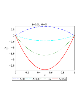
(a) Effect of A on $f^{\prime}(x)$

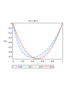
(b) Effect of S on $f^{\prime}(x)$

Figure 1: Effect of A and S on $f^{\prime}(x)$ for the suction cases, Example 1.

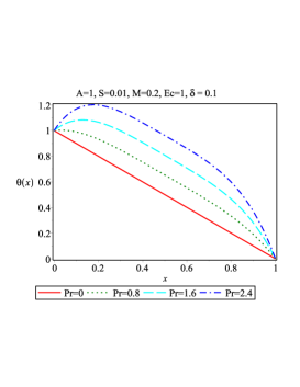
(a) Effect of Pr on $\theta(x)$

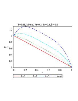
(b) Effect of A on $\theta(x)$

Figure 3: Effect of Pr and A on $\theta(x)$ for the suction cases, Example 1.

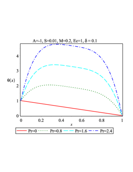
(a) Effect of Pr on $\theta(x)$

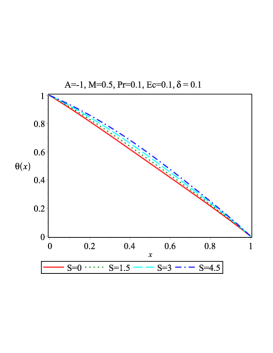
(b) Effect of S on $\theta(x)$

Figure 4: Effect of Pr and S on $\theta(x)$ for the injection cases, Example 1.

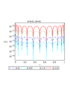
(a) Effect of A on $f^{\prime}(x)$

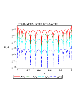
(b) Effect of A on $\theta(x)$

Figure 5: Logarithm graphs of residual error by effects of $A$ on $f^{\prime}(x)$ and $\theta(x)$ for the suction cases with $N=15$, Example 1.

Finally, we generate $2N+2$ algebraic equations, therefore by solving above equations the unknown vectors $F$ and $C$ are achieved.
Effects of deformation parameter S and porosity parameter A are displayed in Figs. (1) and (2).
Fig. (3) shows the influences of flow parameters (in suction case) on the temperature profile. Fig. (4) shows the influences of physical parameters on velocity and temperature distributions in the case of injection.
Fig.(5) shows residual error by the SBT method with $N=15$ on $f^{\prime}(x)$ and $\theta(x)$ for the suction cases.
Tables (1) and (2) show a comparison between the given values $f^{\prime}(x)$ and $\theta(x)$ by the variational iteration method (VIM)refExapmle01 and the SBT methods with $N=15$ for $A=0.1,S=0.1,M=0.2,Pr=0.3,Ec=0.2$ and $\delta=0.1$. It is evident from the table that the present method is efficiency and accuracy of VIM method. Table 3 displays the numerical values of Nusselt number of different values of flow parameters.

Example 2: In this example, we consider the following Lane-Emden type equation on the interval $[0,3]$ as follows refBesselPol13 :

$$y^{\prime\prime}(x)+\frac{2}{x}y^{\prime}(x)-2(2x^{2}+3)y(x)=0,~{}~{}~{}~{}0\leqslant x\leqslant 3,$$ (33)

with the initial conditions

$$y(0)=1,~{}~{}~{}~{}~{}y^{\prime}(0)=0,$$ (34)

The exact solution of this problem is

$$y(x)=e^{x^{2}}.$$ (35)

To solve this example, we approximate $y^{\prime\prime}(x)$ functions by $N+1$ basis of the Bessel polynomials on the interval $[0,3]$ as bellows:

$$y^{\prime\prime}(x)\simeq\sum_{i=0}^{N}{a_{i}Q_{i}(x)}=A^{T}Q(x)$$ (36)

where $A=[a_{0},a_{1},...,a_{N}]^{T}.$ By using Eqs. (13) and (20) we have:

$$x=X(x)^{T}w=Q(x)^{T}\underbrace{(\textbf{M}^{-1})^{T}w}_{\text{U}}=Q(x)^{T}U,$$

$$(2x^{3}+3x)=X(x)^{T}r=Q(x)^{T}\underbrace{(\textbf{M}^{-1})^{T}r}_{\text{Z}}=Q(x)^{T}Z,$$

$$1=X(x)^{T}p=Q(x)^{T}\underbrace{(\textbf{M}^{-1})^{T}p}_{\text{V}}=Q(x)^{T}V,$$

For approximating the solution $y^{\prime}(x)$ and $y(x)$, we apply one and two-time integration on both sides Eq. (4):

$$\int_{0}^{x}y^{\prime\prime}(x)dx=y^{\prime}(x)-y^{\prime}(0)\simeq\int_{0}^{x}A^{T}Q(x)dx\Rightarrow y^{\prime}(x)\simeq A^{T}\textbf{I}Q(x),$$

$$y^{\prime\prime}(x)x=A^{T}Q(x)Q(x)^{T}U\simeq A^{T}\tilde{U}Q(x),$$

$$\int_{0}^{x}y^{\prime}(x)dx=y(x)-y(0)\simeq\int_{0}^{x}A^{T}\textbf{I}Q(x)dx-1$$

$$\Rightarrow y(x)=A^{T}\textbf{I}^{2}Q(x)+V^{T}Q(x)=\underbrace{(A^{T}\textbf{I}^{2}+V^{T})}_{\text{L}}Q(x)=L^{T}Q(x),$$

$$y(x)(2x^{3}+3x)=L^{T}Q(x)Q(x)^{T}Z\simeq L^{T}\tilde{Z}Q(x),$$

where $w=[0,1,0,0,...,0]^{T}$, $r=[0,3,0,2,0,...,0]^{T}$ and $p=[1,0,0,...,0]^{T}$. Therefore, Eq. (33) can be rewritten as:

$$A^{T}\tilde{U}Q(x)+2A^{T}\textbf{I}Q(x)-2L^{T}\tilde{Z}Q(x)=0,$$ (37)

As in a typical Tau method refExapmle02 , we have:

$$A^{T}\tilde{U}+2A^{T}\textbf{I}-2L^{T}\tilde{Z}=0.$$ (38)

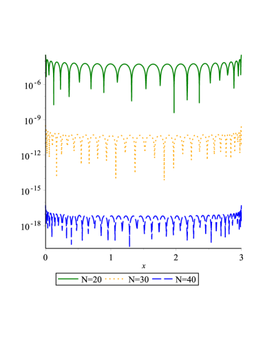
Figure 6: Logarithm graphs of absolute error function, Example 2.

Finally, we generate $N+1$ algebraic equations, therefore by solving above equations the unknown vector $A$ is achieved.
Table (4) reports the comparison of $y(x)$ given by exact value, the Hermite functions collocation (HFC) method applied by Parand et al. Parand.Dehghan.Communications and the proposed method in this paper with $N=40$ . The absolute error graphs of Lane-Emden equation obtained by present method for $N=20,30$ and $40$ are shown in Figure (6).

Example 3: We consider the following nonlinear Abel equation on the interval $[0,1]$ as follows:

$$y^{\prime}(x)=sin(x)y^{3}(x)-xy^{2}(x)+x^{2}y(x)-x^{3},~{}~{}~{}~{}0\leqslant x\leqslant 1,$$ (39)

with the boundary condition

$$y(0)=0.$$ (40)

To solve this example, we approximate $y^{\prime}(x)$ functions by $N+1$ basis of shifted Bessel polynomials on the interval $[0,1]$ as bellows:

$$y^{\prime}(x)\simeq\sum_{i=0}^{N}{a_{i}Q_{i}(x)}=A^{T}Q(x),$$ (41)

where $A=[a_{0},a_{1},...,a_{N}]^{T}.$ By using Eqs. (13) and (20) we have:

$$x=X(x)^{T}w=Q(x)^{T}\underbrace{(\textbf{M}^{-1})^{T}w}_{\text{U}}=Q(x)^{T}U,$$

$$x^{2}=X(x)^{T}r=Q(x)^{T}\underbrace{(\textbf{M}^{-1})^{T}r}_{\text{Z}}=Q(x)^{T}Z,$$

$$x^{3}=X(x)^{T}p=Q(x)^{T}\underbrace{(\textbf{M}^{-1})^{T}p}_{\text{V}}=Q(x)^{T}V,$$

$$sin(x)=Q(x)^{T}S,$$

$$y(x)=A^{T}\textbf{I}Q(x),$$

$$y^{2}(x)x=\Big{(}A^{T}\textbf{I}Q(x)Q(x)^{T}\underbrace{\textbf{I}^{T}A}_{\text{W}}\Big{)}Q(x)^{T}U\simeq A^{T}\textbf{I}\tilde{W}\tilde{U}Q(x),$$

$$y(x)x^{2}=A^{T}\textbf{I}Q(x)Q(x)^{T}Z\simeq A^{T}\textbf{I}\tilde{Z}Q(x),$$

$$y^{3}(x)sin(x)=\Big{(}A^{T}\textbf{I}\tilde{W}Q(x)Q(x)^{T}\underbrace{\textbf{I}^{T}A}_{\text{W}}\Big{)}Q(x)^{T}S\simeq A^{T}\textbf{I}\tilde{W}^{2}\tilde{S}Q(x),$$

where $w=[0,1,0,0,...,0]^{T}$, $r=[0,0,1,0,...,0]^{T}$, $p=[0,0,0,1,0,...,0]^{T}$ and $S^{T}=\langle sin(x),Q^{T}(x)\rangle_{w}\langle Q(x),Q^{T}(x)\rangle_{w}^{-1},$.
Therefore, Eq. (39) can be rewritten as:

$$A^{T}Q(x)-A^{T}\textbf{I}\tilde{W}^{2}\tilde{S}Q(x)+A^{T}\textbf{I}\tilde{Z}Q(x)-A^{T}\textbf{I}\tilde{Z}Q(x)+V^{T}Q(x)=0,$$ (42)

As in a typical Tau method refExapmle02 , we have:

$$A^{T}-A^{T}\textbf{I}\tilde{W}^{2}\tilde{S}+A^{T}\textbf{I}\tilde{Z}-A^{T}\textbf{I}\tilde{Z}+V^{T}=0,$$ (43)

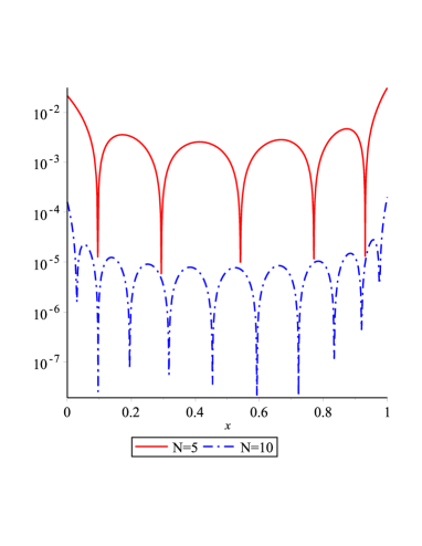
Figure 7: Logarithm graphs of residual error function, Example 3.

In this step, we generate $N+1$ algebraic equations, therefore by solving above equations the unknown vector $A$ is achieved.
The residual error graphs of the nonlinear Abel equation obtained by present method for $N=5$ and $10$ are shown in Figure (7). Table (5) displays given values $y(x)$ by the fractional order of the Chebyshev orthogonal functions (FCFs) collocation method used by parand et al. Delkhosh.Nikarya , the present method and the residual error with $N=10$.

Example 4: Consider the nonlinear the standard Lane-Emden problem

$$y^{\prime\prime}(x)+\frac{1}{x}y^{\prime}(x)+y^{2}=0,~{}~{}~{}~{}0\leqslant x\leqslant 2$$ (44)

with the boundary condition

$$y(0)=1,~{}~{}~{}y^{\prime}(0)=0.$$ (45)

Thus, the solution of the Lane-Emden equation is obtained by the SBT method with $N=8$ and $N=12$.

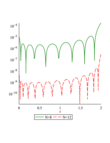
Figure 8: Logarithm graphs of residual error function, Example 4.

The residual error graphs of the nonlinear standard Lane-Emden obtained by the present method for $N=8$ and $12$ are shown in Figure (8). Table (6) reports the comparison of the obtained values $y(x)$ by the present method with $N=12$, Horedt refExapmle04 , the Bessel orthogonal functions collocation (BFC) method utilized by Parand et al. refBesselPol05 and the Chebyshev orthogonal functions (GFCFs) collocation method proposed by Parand et al. Parand.Delkhosh.Teknoligy .

Example 5: ّFinally, consider the boundary-value the Troesch’s problem

$$y^{\prime\prime}(x)=\gamma\sinh(\gamma y(x)),~{}~{}~{}~{}0\leqslant x\leqslant 1,$$ (46)

with the boundary conditions

$$y(0)=0,~{}~{}~{}y(1)=1,$$ (47)

We approximate $y(x)$ functions by $N+1$ basis of shifted Bessel polynomials on the interval $[0,1]$ as bellows:

$$y(x)\simeq\sum_{i=0}^{N}{a_{i}Q_{i}(x)}=A^{T}Q(x)$$

where $A=[a_{0},a_{1},...,a_{N}]^{T}$ .

By using the SBT technique described in the paper, we can generate a set of linear algebraic equations as follows:

$$A^{T}\textbf{D}^{2}-\gamma(\gamma A^{T}+\frac{\gamma^{3}}{3!}A^{T}\tilde{A}^{2}+\frac{\gamma^{5}}{5!}A^{T}\tilde{A}^{4})=0,$$ (48)

where $Q(x)Q(x)^{T}A\simeq\tilde{A}Q(x)$.

To satisfy the boundary conditions Eq. (47), we have substituted the following equations in two rows of Eq. (48):

$$y(0)=A^{T}Q(0)=0,~{}~{}~{}y(1)=A^{T}Q(0)=1.$$ (49)

Table (7) displays the comparison of the obtained values $y(x)$ by the modified non-linear shooting method (MNLSM) applied by Alias Alias.Teknology , the numerical scheme based on the modified homotopy perturbation technique used by Feng.Computation and the present method with $N=10$ and $\gamma=0.5$.

5 Conclusion

The shifted Bessel Tau (SBT) method is a useful technique for solving ordinary differential equations. Numerical programs using this method are often considerably faster with greater accuracy than other standard techniques such as the variational iteration method, shooting method and homotopy perturbation technique. Interest in the Tau method, for a long time regarded only as a tool for the construction of accurate approximations of a very restricted class of functions, has been enhanced. In this investigation, the Bessel polynomials operational matrices of integration, differentiation, and product are derived. A general procedure for the formulation of these matrices is given. By utilizing the operational matrices and the Tau method, we reduce the solution of the original equations to the solution of a nonlinear algebraic equation system. Therefore, all of these equations can be solved by Newton method for the unknown coefficients. Some problems with initial or boundary conditions are considered in one dimensional contexts, although the proposed technique can be easily implemented for two and three dimensional problems. The main advantage of the present method is its simplicity and convenience for computer algorithms. Illustrative examples demonstrate the validity and applicability of the present method.

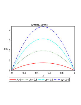
(a) Effect of A on $f^{\prime}(x)$

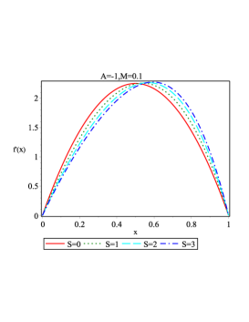
(b) Effect of S on $f^{\prime}(x)$

Figure 2: Effect of A and S on $f^{\prime}(x)$ for the injection cases, Example 1.

Table 1: Comparison of the obtained values $f^{\prime}(x)$ by the variational iteration method (VIM)refExapmle01 and the present method, Example 1.

$x$	Bessel Tau method	VIMrefExapmle01	$Res(x)$
0.2	0.384801280290557	0.384801	1.39535e-12
0.4	0.575554143054330	0.575554	8.21911e-14
0.6	0.575174675564395	0.575174	1.90287e-12
0.8	0.384040432902588	0.384040	1.91562e-12

Table 2: Comparison of the obtained values $\theta(x)$ by the variational iteration method (VIM)refExapmle01 and the present method, Example 1.

$x$	Bessel Tau method	VIMrefExapmle01	$Res(x)$
0.2	0.806144282850332	0.806144	8.25970e-14
0.4	0.607022034290869	0.607022	7.26187e-14
0.6	0.407003862839112	0.407004	7.24240e-14
0.8	0.206120555470330	0.206121	8.19659e-14

Table 3: Comparison of values of Nusselt number $(1-at)^{1/2}Nu$ for different values of $Pr,Ec$, and $\delta$ when $A=0.1,~{}S=0.1,~{}M=0.2$ by the present method with $N=15$ and the variational iteration method (VIM) refExapmle01 , Example 1.

Pr	Ec	$\delta$	$(1-at)^{1/2}Nu$	VIM refExapmle01
0.0	0.2	0.1	1.00000000000000000	1.00000
0.1			1.01893685003010788	1.01894
0.2			1.03787156909761297	1.03787
0.3	0.0		0.99859957004178043	0.99860
	0.2		1.05680415677248143	1.05680
	0.4		1.11500874350318244	1.11501
	0.3	0.0	1.08487154864359339	1.08487
		0.5	1.11074408599955706	1.11074
		1.0	1.18836169806744806	1.18836

Table 4: Comparison of the obtained values $y(x)$ by exact value, HFC method Parand.Dehghan.Communications and the present method with $N=40$, Example 2.

$x$	Exact value	HFC Parand.Dehghan.Communications	Peresent method
0.01	1.00010000500016667083	1.0000999826	1.00010000500016665722
0.02	1.00040008001066773341	1.0004000642	1.00040008001066774881
0.05	1.00250312760579508497	1.0025031064	1.00250312760579507309
0.10	1.01005016708416805754	1.0100501492	1.01005016708416805546
0.20	1.04081077419238822675	1.0408107527	1.04081077419238822399
0.50	1.28402541668774148407	1.2840253862	1.28402541668774147818
0.70	1.63231621995537897012	1.6323161777	1.63231621995537896294
0.80	1.89648087930495135334	1.8964808279	1.89648087930495136037
0.90	2.24790798667647141917	2.2479078937	2.24790798667647141232
1.00	2.71828182845904523536	2.7182819166	2.71828182845904524184
1.5	9.48773583635852572055	—	9.48773583635852572300
2.0	54.5981500331442390781	—	54.5981500331442390719
2.5	518.012824668342025939	—	518.012824668342025947
3.0	8103.08392757538400770	—	8103.08392757538400765

Table 5: Numerical given values $y(x)$ by FCFs collocation method Delkhosh.Nikarya and the present method with $N=10$, Example 3.

$x$	FCFs Delkhosh.Nikarya	Present method	Residual error
0.1	-2.500e-5	-2.541201381e-5	2.13471e-6
0.2	-4.004e-4	-4.000957821e-4	1.42107e-6
0.3	-2.032e-3	-2.033184449e-3	3.48798e-6
0.4	-6.459e-3	-6.459447204e-3	7.35610e-6
0.5	-1.591e-2	-1.591376982e-2	6.64911e-6
0.6	-3.346e-2	-3.346334651e-2	1.36557e-6
0.7	-6.327e-2	6.327405918e-2	4.86862e-6
0.8	-1.111e-1	-1.111347323e-1	9.41866e-6
0.1	-1.855e-1	1.855105463e-1	1.23827e-5
1.0	-2.999e-1	-2.999554921e-1	1.98917e-4

Table 6: Comparison of the obtained values $y(x)$ by the present method with $N=12$, Horedt refExapmle04 , BFC method refBesselPol05 and GFCFs collocation method Parand.Delkhosh.Teknoligy , Example 4.

$x$	Present method	Horedt refExapmle04	BFC refBesselPol05	GFCFs Parand.Delkhosh.Teknoligy
0.1	0.998334998549872	0.9983350	0.99833499854	0.99833499986
0.3	0.985133946938390	–	–	–
0.5	0.959352715810926	0.9593527	0.95935271580	0.95935271585
0.7	0.922170348514590	–	–	–
1.0	0.848654111411546	0.8486541	0.84865411140	0.84865409603
1.5	0.695367147241325	–	–	–
2.0	0.529836429310169	–	–	–

Table 7: Comparison of the obtained values $y(x)$ by Alias Alias.Teknology , Feng Feng.Computation and the present method with $N=10$ and $\gamma=0.5$, Example 5.

$x$	Alias Alias.Teknology	Feng Feng.Computation	Present method	Residual eroor
0.1	0.09597247	0.0959477541	0.095944350620621	3.18e-13
0.2	0.19218506	0.1921352537	0.192128750320282	6.98e-12
0.3	0.28887905	0.2888034214	0.288794404891654	1.04e-10
0.4	0.38629807	0.3861955524	0.386184851707410	7.44e-10
0.5	0.48441684	0.4845585473	0.484547171441282	3.63e-09
0.6	0.58428140	0.5841442013	0.584133256467667	1.49e-08
0.7	0.68525684	0.6852105701	0.685201157498259	5.56e-08
0.8	0.78807945	0.7880234321	0.788016532411673	1.91e-07
0.9	0.89292601	0.8928578710	0.892854224345211	6.07e-07

References

- (1) B.A. Finlayson, The Method of Weighted Residuals and Variational Principles. Academic Press, New York (1972).
- (2) S. Kazem, M. Shaban, J.A. Rad, Solution of Coupled Burger’s equation based on operational matrices of d-dimensional orthogonal functions, Z. Naturforsch. A, 67 (5), 267-274.
- (3) K. Parand, M. Dehghan, F. Baharifard, Solving a laminar boundary layer equation with the rational gegenbauer functions. Appl. Math. Model., 37 (2013) 851-863 .
- (4) E. Doha, A. Bhrawy, Efficient spectral-galerkin algorithms for direct solution for second-order differential equations using jacobi polynomials. Numer. Algorithm, 42 (2006) 137-164.
- (5) S. Shateyi, S.S. Motsa, Y. Khan, A new piecewise spectral homotopy analysisof the Michaelis-Menten enzymatic reactions model. Numer. Algorithm, 66 (2014) 495-510.
- (6) C. Lanczos, Trigonometric interpolation of empirical and analytical functions. J. Math. Phys., 17 (1938) 123-199.
- (7) A. Saadatmandi, M. Dehghan, A Tau approach for solution of the space fractional diffusion equation. Comput. Math. Appl., 62 (2011) 1135-1142.
- (8) A. Yildirim, S. Sezer, Y. Kaplan, Analytical approach to Boussinesq equation with space and timefractional derivatives, Int. J. Numer. Meth. Fluids, 66 (2011) 1315-1324.
- (9) J. H. He, Application of homotopy perturbation method to nonlinear wave equations, Chaos Soliton Fract, 26 (2005) 695-700.
- (10) S. Kazem, J. Rad, K. Parand, Radial basis functions methods for solving Fokker-Planck equation, Eng. Anal. Bound. Elem., 36 (2012)181-189.
- (11) K. Parand, M. Shahini, M. Dehghan, Rational Legendre pseudospectral approach for solving nonlinear differential equations of Lane-Emden type, J. Comput. Phys., 228 (2009) 8830-8840.
- (12) S. Abbasbandy, E. Shivanian, A new analytical technique to solve Fredholm’s integral equations, Numer. Algorithms, 56 (2011) 27-43.
- (13) S. J. Liao, Series solution of nonlinear eigenvalue problems by means of the homotopy analysis method, Nonlinear Anal. Real, 10 (2009) 2455-2470.
- (14) K. Parand, M. Razzaghi, Rational Legendre approximation for solving some physical problems on semi-infinite intervals, Phys. Scripta, 69 (2004) 353-357.
- (15) K. Parand, M. Razzaghi, Rational Chebyshev tau method for solving higher-order ordinary differential equations, Int. J. Comput. Math., 81 (2004) 73-80.
- (16) S. Yousefi, M. Dehghan, The use of He’s variational iteration method for solving variational problems, Int. J. Comput. Math., 87 (2010) 1299-1314.
- (17) A. Wazwaz, A reliable treatment of singular Emden-Fowler initial value problems and boundary value problems, Appl. Math. Comput., 217 (2011) 10387-10395.
- (18) A. Saadatmandi, M. Dehghan, A new operational matrix for solving fractional-order differential equations, Comput. Math. Appl., 59 (2010) 1326-1336.
- (19) J. S. Gu, W. S. Jiang, The haar wavelets operational matrix of integration, Int. J. Syst. Sci., 27 (1996) 623-628.
- (20) I. Horng, J. Chou, Shifted Chebyshev direct method for solving variational problems, Int. J. Syst. Sci., 16 (1985) 855-861.
- (21) M. Razzaghi, S. Yousefi, The legendre Wavelets operational matrix of integration, Int. J. Syst. Sci., 32 (2001) 495-502.
- (22) M. Razzaghi, S. Yousefi, Sine-Cosine Wavelets operational matrix of integration and its applications in the calculus of variations, Int. J. Syst. Sci., 33 (2002) 805-810.
- (23) S. A. Yousefi, M. Behroozifar, Operational matrices of bernstein polynomials and their applications, Int. J. Syst. Sci., 41 (2010) 709-716.
- (24) M. Razzaghi, M. Razzaghi, Fourier series direct method for variational problems, Int. J. Control, 48 (1988) 887-895.
- (25) M. Razzaghi, M. Razzaghi, Taylor series analysis of time-varying multi-delay systems, Int. J. Control, 50 (1989) 183-192.
- (26) M. Razzaghi, M. Razzaghi, Shifted-Jacobi series direct method for variational problems, Int. J. Syst. Sci., 20 (1989) 1119-1129.
- (27) K. Parand, M. Razzaghi, Rational Chebyshev tau method for solving Volterra’s population model, Appl. Math. Comput., 149 (2004) 893-900.
- (28) K. Parand, M. Razzaghi, Rational Chebyshev tau method for solving higher-order ordinary differential equations, Int. J. Comput. Math., 81 (2004) 73-80.
- (29) K. Parand, H. Yousefi, M. Delkhosh, A. Ghaderi,A novel numerical technique to obtain an accurate solution to the Thomas-Fermi equation, Eur. Phys. J. Plus, 131 (7), 1-16.
- (30) K Parand, P Mazaheri, M Delkhosh, A Ghaderi, New numerical solutions for solving Kidder equation by using the rational Jacobi functions, SeMA J., (2016) doi:10.1007/s40324-016-0103-z.
- (31) E. H. Doha, A. H. Bhrawy and S. S. Ezz-Eldien, A new Jacobi operational matrix: An application for solving fractional differential equations, Appl. Math. Model., 36 (2012) 4931-4943.
- (32) S. A. Yousefi, H. Jafari and M. A. Firoozjaeeand S. Momani and C. M. Khaliqued, Application of Legendre wavelets for solving fractional differential equations, Comput. Math. Appl., 62 (2011) 1038-1045.
- (33) S. A. Yousefi, F. Khellat,The linear Legendre mother wavelets operational matrix of integration and its application, J. Franklin Inst., 343 (2006) 181-190.
- (34) S. A. Yousefi, M. Behroozifar, M. Dehghan, Numerical solution of the nonlinear age-structured population models by using the operational matrices of Bernstein polynomials, Appl. Math. Modell., 36 (2012) 945-963.
- (35) S. A. Yousefi, M. Behroozifar, M. Dehghan, The operational matrices of Bernstein polynomials for solving the parabolic equation subject to specification of the mass, J. Comput. Appl. Math., 335 (2011) 5272-5283.
- (36) A. H. Bhrawy, The operational matrix of fractional integration for shifted Chebyshev polynomials, Appl. Math. Lett., 26 (2013) 25-31.
- (37) H. R. Marzban, M. Razzaghi, Optimal control of linear delay systems via hybrid of block-pulse and Legendre polynomials, J. Franklin Inst., 341 (2004) 279-293.
- (38) H. R. Marzban, M. Shahsiah, Solution of piecewise constant delay systems using hybrid of block-pulse and Chebyshev polynomials, Optim. Contr. Appl. Met., 32 (2011) 647-659.
- (39) M. Lakestani, M. Dehghan, S. I. Pakchin, The construction of operational matrix of fractional derivatives using B-spline functions, Commun. Nonlinear. Sci. Numer. Simulat., 17 (2012) 1149-1162.
- (40) S. Kazem, M. Shaban, J. A. Rad, Solution of the coupled burgers equation based on operational matrices of d-dimensional orthogonal functions, Z. Naturforsch. A., 67 (2012) 267-274.
- (41) S. Nemati, P. M. Lima, Y. Ordokhani, Numerical solution of a class of two-dimensional nonlinear Volterra integral equations using Legendre polynomials, J. Comput. Appl. Math., 242 (2013) 53-69.
- (42) K. Parand, M.i Delkhosh, Solving Volterra’s population growth model of arbitrary order using the generalized fractional order of the Chebyshev functions, Ricerch. Mat., 65 (2016) 307-328.
- (43) W.W. Bell, Special functions for scientists and engineers, D. Van Nostrand Company, CEf Canada, 1967.
- (44) K. Parand, M. Nikarya, J.A. Rad, F. Baharifard, A new reliable numerical algorithm based on the first kind of Bessel functions to solve Prandtl-Blasius laminar viscous flow over a semi-infinite flat plate, Z. Naturforsch. A, 67 (2012) 665-673.
- (45) K. Parand, M. Nikarya, J.A. Rad, Solving non-linear Lane-Emden type equations using Bessel orthogonal functions collocation method, Celest. Mech. Dyn. Astr., 116 (2013) 97-107.
- (46) M. Delkhosh, The conversion a Bessel’s equation to a self-adjoint equation and applications, World Appl. Sci. J., 15, 1687-1691 (2011).
- (47) N. Sahin, S. Yuzbasi, M. Gulsu, A collocation approach for solving systems of linear Volterra integral equations with variable coefficients, Comput. Math. Appl., 62 (2011) 755-769.
- (48) S. Yuzbasi, M. Sezer, A numerical method to solve a class of linear integro-differential equations with weakly singular kernel, Math. Method Appl. Sci., 35 (2012) 621-632.
- (49) S. Yuzbasi, N. Sahin, M. Sezer, Bessel polynomial solutions of high-order linear Volterra integro-differential equations, Comput. Math. Appl., 62 (2011) 1940-1956.
- (50) S. Yuzbasi, A numerical approach for solving a class of the nonlinear Lane-Emden type equations arising in astrophysics, Math. Method Appl. Sci., 34 (2011) 2218-2230.
- (51) S. Yuzbasi, Bessel collocation approach for solving continuous population models for single and interacting species, Appl. Math. Model., 36 (2012) 3787-3802.
- (52) S. Yuzbas, A collocation method based on the Bessel functions of the first kind for singular perturbated differential equations and residual correction, Math. Method Appl. Sci., 38 (2015) 3033-3042.
- (53) E. Tohidi, H. Nik, A Bessel collocation method for solving fractional optimal control problems, Appl. Math. Model., 39 (2015) 455-465.
- (54) K. Parand, A. Ghaderi, H. Yousefi, M. Delkhosh, A new approach for solving nonlinear Thomas-Fermi equation based on fractional order of rational Bessel functions, Electron. J. Differential Equations, 2016 (2016), No. 331, pp. 1-18.
- (55) Z. Odibat, S. Momani, An algorithm for the numerical solution of differential equations of fractional order, J. Appl. Math. Info., 26 (2008) 15-27.
- (56) S.I. Khan, N. Ahmed, U. Khan, S. Ullah Jan, S.T. Mohyud-Din, Heat transfer analysis for squeezing flow between parallel disks, J. Egypt. Math. Society, 23 (2015) 445-450.
- (57) D. Gottlieb, M. Hussaini, S. Orszg, Theory and applications of spectral methods in spectral methods for partial differential equations, SIAM, Philadelphia, 1984.
- (58) K. Parand, M. Delkhosh, M. Nikarya, Novel Orthogonal Functions for Solving Differential Equations of Arbitrary Order, Tbilisi Math. J., 10 (2017) 31-55.
- (59) G. P. Horedt, Polytropes: Applications in Astrophysics and Related Fileds. Kluwer, Dordecht (2004).
- (60) K. Parand, M. Delkhosh, An effective numerical method for solving the nonlinear singular Lane-Emden type equations of various orders, J. Teknologi, 79 (2017) 25-36 .
- (61) K. Parand, M. Dehghan, A. R. Rezaei, S. M. Ghaderi, An approximation algorithm for the solution of the nonlinear Lane-Emden type equations arising in astrophysics using Hermite functions collocation method, Comp. Phys. Commun., 181 (2010) 1096-1108.
- (62) N. Alias, A. Manaf, A. Ali, M. Habib, Solving Troesch’s problem by using modified nonlinear Shooting method, J. Teknologi, 78 (2016) 45-52.
- (63) X. Feng, L. Mei, G. He, An efficient algorithm for solving Troesch’s problem, Appl. Math. Comp., 189 (2007) 500-507.