The Intelligent Driver Model with Stochasticity – New Insights Into Traffic Flow Oscillations

Abstract

Traffic flow oscillations, including traffic waves, are a common yet incompletely understood feature of congested traffic. Possible mechanisms include traffic flow instabilities, indifference regions or finite human perception thresholds (action points), and external acceleration noise. However, the relative importance of these factors in a given situation remains unclear. We bring light into this question by adding external noise and action points to the Intelligent Driver Model and other car-following models thereby obtaining a minimal model containing all three oscillation mechanisms. We show analytically that even in the subcritical regime of linearly stable flow (order parameter $\epsilon<0$), external white noise leads to spatiotemporal speed correlations “anticipating” the waves of the linearly unstable regime. Sufficiently far away from the threshold, the amplitude scales with $(-\epsilon)^{-0.5}$. By means of simulations and comparisons with experimental car platoons and bicycle traffic, we show that external noise and indifference regions with action points have essentially equivalent effects. Furthermore, flow instabilities dominate the oscillations on freeways while external noise or action points prevail at low desired speeds such as vehicular city or bicycle traffic. For bicycle traffic, noise can lead to fully developed waves even for single-file traffic in the subcritical regime.

1 Introduction

Traffic flow oscillations, including stop-and-go traffic, are a common phenomenon in congested vehicular traffic [1, 2, 3, 4, 5]. Conventionally, this phenomenon is described in terms of linear or nonlinear string or flow instabilities [6, 7, 8] which are typically triggered by a local persistent perturbation, e.g., lane changes near a bottleneck [2]. In another approach, the flow oscillations are traced back to indifference regions of the human driver [9, 10] or to finite perception thresholds leading to abrupt acceleration changes at discrete “action points” [11, 12]. Related to this are finite attention spans [13, 14]. It has also ben proposed that the oscillations may be caused by event-oriented changes of the driving style switching, e.g., between “timid” and “aggressive” [15], or, related to this, by over- and underreactions [16]. Finally, direct external additive or multiplicative acceleration noise (e.g., caused by perception errors) is postulated to drive the oscillations. This line of reasoning is typically modelled by cellular automata (e.g., [17]) which need some sort of stochasticity, anyway, for a proper specification. However, there are also approaches to incorporate acceleration noise into time-continuous car-following models leading to stochastic differential equations [14, 18]. One of the simplest approaches is the “Parsimonious Car-Following Model” (PCF model) [19] which adds white acceleration noise to the free-acceleration part of Newell’s car-following model with bounded acceleration [20] and, as [14], also provides explicit numerical stochastic update rules by integrating the stochastic differential equation over one time step.

While all of the above approaches can explain certain observations, it remains an open question whether these approaches are connected with each other, and if so, in which way. Another open problem is to identify the situations where oscillations are caused predominantly by flow instabilities, by indifference regions, or by noise.

In this contribution, we bring light into these questions by proposing a general scheme for adding noise and indifference regions (in form of action points) to a class of deterministic acceleration-based car-following models. Suitable underlying models include the Intelligent Driver Model (IDM) [21], the Full Velocity Difference Model (FVDM) [22], or Newell’s car-following model [23] with bounded accelerations [20]. In this way, we obtain a minimal model containing all three mechanisms which we then analyze analytically and numerically. The focus is on the generic instability mechanisms and their relative importance rather than on specific car-following models.

The rest of the paper is organized as follows: In the next section, we specify the minimal model. In Section 3, we introduce the order parameter $\epsilon$ denoting the relative distance to linear string instability and analytically derive, as a function of $\epsilon$, the statistical fluctuation properties induced by white noise, including spectral, modal, and overall intensity of the vehicle gap and speed fluctuations, and the associated spatiotemporal correlations. In the Sections 4 and 5, we investigate the oscillation mechanisms for high-speed and low-speed traffic (cars and bicycles, respectively), and compare the results with experimental observations. Finally, Section 6 concludes with a discussion.

2 Model Specification

We consider general stochastic time-continuous car-following models of the form

$$\dot{v}_{n}=f(s_{n},v_{n},v_{l})+\xi_{n}(t),\quad\mbox{$\langle\xi_{n}(t)\rangle$}=0,\quad\mbox{$\langle\xi_{n}(t)\xi_{m}(t^{\prime})\rangle$}=Q\delta_{nm}\delta(t-t^{\prime}).$$ (1)

Here, $f(\cdot)$ denotes the acceleration function of the underlying car-following model for vehicle $n$ as a function of the (bumper-to-bumper) gap $s_{n}$, the speed $v_{n}$, and the leader’s speed $v_{l}$. Time delays in the independent variables representing reaction times such as in Newell’s Car-Following Model [23] are allowed. The white acceleration noise $\xi_{n}(t)$ is completely uncorrelated in time and between vehicles (the Kronecker symbol $\delta_{nm}=1$ for $n=m$ and zero, otherwise; $\delta(t-t^{\prime})$ denotes Dirac’s delta distribution), and has the intensity $Q$. Model (1) can be seen as a simplistic special case of the Human Driver Model (HDM) [14]. Notice that, when starting with a deterministic initial state $v_{n}(0)$ at $t=0$, integration of the stochastic differential equation (1) leads, in the limit $t\to 0$, to a Gaussian speed distribution whose expectation and variance are given by (see, e.g., [24])

$$\mbox{$\langle v_{n}(t)\rangle$}=v_{n}(0)+ft,\quad\mbox{$\langle(v_{n}(t)-(v_{n}(0)+ft)^{2}\rangle$}=Qt$$ (2)

where the variance is independent of $f$. Consequently, $Q$ has the unit $\mathrm{m^{2}/s^{3}}$. By chosing a deterministic car-following model with the ability for string instability, e.g., the Intelligent Driver Model (IDM) [21] or the Full Velocity Difference Model (FVDM) [22], the model (1) contains the two oscillation-inducing factors noise and string instability. We introduce the third factor, indifference regions in the form of action points, by updating the deterministic acceleration to the actual value given by $f(\cdot)$ only, if

$$\left|f(s_{i}(t),v_{i}(t),v_{l}(t))-f(s_{i}(t^{\prime}),v_{i}(t^{\prime}),v_{l}(t^{\prime}))\right|>\Delta a,\quad\Delta a\sim U(0,\Delta a_{\rm max}).$$ (3)

Here, $t^{\prime}$ is the time of the last change (action point) and $\Delta a$ is a uniformly distributed random number drawn at the last action point whose maximum value must be well below the maximum acceleration capability of the deterministic model.

Since characterizing action points according to model (3) is a novel proposition in itself, we first show how the mechanism works by displaying typical instances of the resulting acceleration time series (Fig. 1). As expected, the drivers drive at constant accelerations, most of the time. These episodes with typical irregular durations between 1 s and 20 s are separated by “action points” where the acceleration is changed by a variable amount whose maximum is given by the parameter $\Delta a_{\rm max}$. Notice that both the irregular durations and increments agree with observations [12].

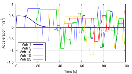
Fig. 1: Visualization of the action points (maximum step $\Delta a_{\rm max}=1.0\,\mathrm{m/s^{2}}$) by a time series of the accelerations of four platoon vehicles corresponding to Fig. 7(e) and (f). Also shown is the leader (Vehicle 1) accelerating slowly and deterministically to the final speed of 30 km/h.

The Eqs. (1) (or (2)), (3), and a deterministic car-following model specify the proposed minimal model containing all three oscillation factors. Each factor can be controlled by a single parameter. The noise is controlled by the noise intensity $Q$ (typical values are of the order of $0.2\,\mathrm{m^{2}/s^{3}}$), the indifference region by the maximum acceleration step $\Delta a_{\rm max}$ (of the order of $1\,\mathrm{m/s^{2}}$ or less), and the string instability by the relevant parameter of the underlying car-following model, e.g., the maximum acceleration $a$ for the IDM. It is convenient to define the relative distance to the linear threshold $a_{c}$ (see Section 3 below) by the order parameter

$$\epsilon=1-\frac{a}{a_{c}}$$ (4)

keeping the other IDM parameters fixed. A homogeneous deterministic steady state is linearly stable for $\epsilon<0$ (subcritical regime), and linearly string unstable for $\epsilon>0$ (supercritical).

3 Noise-Induced Subcritical Oscillations

In order to analytically determine the linear response to the white acceleration noise, we assume a homogeneous ring road of circumference $L$ with $N$ identical drivers/vehicles such that the global density is given by $\rho=N/L$. Furthermore, we switch off the action points by setting $\Delta a_{\rm max}=0$. We generalize the standard linear stability analysis (see, e.g., Ref. [8]) to include noise. Starting from a homogeneous steady state $v_{n}=v_{e}$ and $s_{n}=s_{e}(v_{e})$ lying on the fundamental diagram, we decompose the gaps and speeds into the steady-state contribution and a small time-dependent perturbation by setting $s_{n}(t)=s_{e}+y_{n}(t)$, $v_{n}(t)=v_{e}+u_{n}(t)$. This leads to the linearized equations

$$\frac{{\rm d}y_{n}}{{\rm d}t}=u_{n-1}-u_{n},\quad\frac{{\rm d}u_{n}}{{\rm d}t}=f_{s}y_{n}+f_{v}u_{n}+f_{l}u_{n-1}+\xi_{n}(t),$$ (5)

where $f_{s}=\frac{\partial f}{\partial s}$, $f_{v}=\frac{\partial f}{\partial v}$, and $f_{l}=\frac{\partial f}{\partial v_{l}}$ are the gradients of the acceleration function $f(\cdot)$ at the deterministic steady state.

The time-dependent parts can be further decomposed into $N$ harmonic eigenmodes of wave number $k=2\pi m/N$, $m=-N/2+1,...,N/2$ (with $|m|$ indicating the number of travelling waves on the ring and $2\pi/|k|$ the number of vehicles per wave) by the ansatz

$$\left(\begin{array}[]{c}y_{n}(t)\\ u_{n}(t)\end{array}\right)=\sum_{k}\left(\begin{array}[]{c}\hat{y}_{k}(t)\\ \hat{u}_{k}(t)\end{array}\right)e^{ink}$$ (6)

where $i=\sqrt{-1}$ is the imaginary unit. Inserting this into (5), we obtain a set of independent pairs of stochastic differential equations for the modes $k$,

$$\begin{array}[]{rcl}\frac{{\rm d}\hat{y}_{k}}{{\rm d}t}&=&\left(e^{-ik}-1\right)\hat{u}_{k},\\ \frac{{\rm d}\hat{u}_{k}}{{\rm d}t}&=&f_{s}\hat{y}_{k}+\left(f_{v}+f_{l}e^{-ik}\right)\hat{u}_{k}+\hat{\xi}_{k}(t),\end{array}$$ (7)

where the noise source now is given by

$$\left\langle\hat{\xi}_{k}(t)\right\rangle=0,\quad\left\langle\hat{\xi}_{k}(t)\hat{\xi}_{l}(t^{\prime})\right\rangle=\frac{Q}{N}\delta_{kl}\delta(t-t^{\prime}).$$ (8)

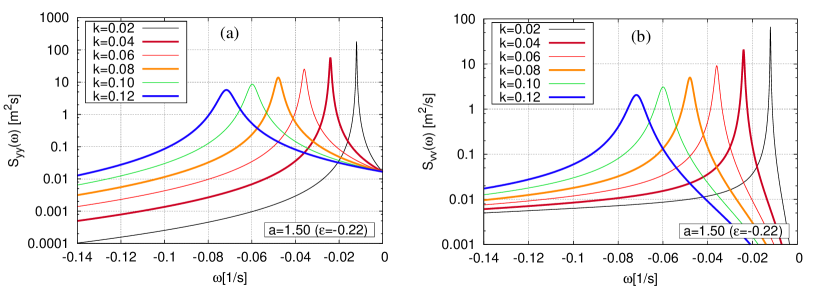
Fig. 2: Steady-state fluctuation spectrum of (a) the speeds, and (b) the gaps for the IDM with the parameters of the main text and white acceleration noise of intensity $Q=0.1\,\mathrm{m^{2}/s^{3}}$. Shown is the spectrum for several modes of dimensionless wavenumber $k$ (number of vehicles $2\pi/k$ per wave). The negative values for $\omega$ indicate an upstream propagation of $-\omega/k$ vehicles per second in the frame comoving with the vehicles. The underlying deterministic steady state is characterized by $v_{e}=48\,\mathrm{km/h}$ corresponding to a density of 36.4 vehicles/km.

Each pair of linear stochastic differential equation (8) can be written in the general form

$$\frac{{\rm d}}{{\rm d}t}\vec{X}_{k}=-{\mbox{ \sf{L}}}_{k})\vec{X}_{k}+\vec{\xi},\quad\mbox{$\langle\vec{\xi}(t)\rangle$}=0,\quad\mbox{$\langle\vec{\xi}(t)\vec{\xi}^{\prime}(t^{\prime})\rangle$}={\mbox{ \sf{D}}}\delta(t-t^{\prime})$$ (9)

where $\vec{X}_{k}=(\hat{y}_{k},\hat{u}_{k})^{\prime}$ denotes the state vector of mode $k$, and

$${\mbox{ \sf{L}}}_{k}=\left(\begin{array}[]{cc}0&1-e^{-ik}\\ -f_{s}&-(f_{v}+f_{l}e^{-ik})\end{array}\right),\quad{\mbox{ \sf{D}}}=\frac{Q}{N}\left(\begin{array}[]{cc}0&0\\ 0&1\end{array}\right),$$ (10)

denote the linear dissipation matrix, and the covariance matrix of the white noise, respectively.

The stationary solutions to (9) consist of zero-mean Gaussian fluctuations which are therefore completely specified by the amplitude and correlation of the state variables as well as the temporal autocorrelation function. Instead of the autocorrelation function, one can also determine the spectral intensity of the gap and speed oscillations of waves of wavenumber $k=2\pi/L$ (where $L$ is the wavelength), i.e., the differential energy content (amplitude squared) contained in waves of wavenumber $k$ at an angular frequency $\omega=2\pi/T$ (where $T$ is the wave period). Remarkably, there exists an analytic solution for the spectral intensity of the stationary fluctuations called the fluctuation-dissipation theorem [24],

$${\mbox{ \sf{S}}}_{k}(\omega)=\left({\mbox{ \sf{L}}}_{k}+i\omega{\mbox{ \sf{1}}}\right)^{-1}{\mbox{ \sf{D}}}\left({\mbox{ \sf{L}}}^{\prime}_{k}-i\omega{\mbox{ \sf{1}}}\right)^{-1}.$$ (11)

Here, ${\mbox{ \sf{S}}}_{k}(\omega)=\tilde{\vec{X}}_{k}(\omega)\tilde{\vec{X}}_{k}^{\prime}(\omega)$ is the spectral intensity with $\tilde{\vec{X}}_{k}(\omega)$ the Fourier transform of $\vec{X}_{k}(t)$, and $\tilde{\vec{X}}_{k}^{\prime}(\omega)$ its transposed complex conjugate. Furthermore, ${\mbox{ \sf{L}}}_{k}^{\prime}$ is the transposed and complex conjugate of the linear matrix ${\mbox{ \sf{L}}}_{k}$. Inserting (10), we finally obtain the subcritical modal fluctuation spectrum

$${\mbox{ \sf{S}}}_{k}(\omega)=\frac{Q}{N|{\mbox{ Det}}({\mbox{ \sf{L}}}+i\omega{\mbox{ \sf{1}}})|^{2}}\left(\begin{array}[]{cc}2(1-\cos k)&i\omega(1-e^{-ik})\\ -i\omega(1-e^{ik})&\omega^{2}\end{array}\right)$$ (12)

where

$$\left|{\mbox{ Det}}({\mbox{ \sf{L}}}+i\omega{\mbox{ \sf{1}}})\right|^{2}=\left(\omega^{2}+\omega f_{l}\sin k-f_{s}(1-\cos k)\right)^{2}+\left(f_{s}\sin k-\omega(f_{v}+f_{l}\cos k)\right)^{2}.$$

The diagonal components are of particular interest. $S_{11}=S_{yyk}(\omega)$ gives the spectral intensity of the gap oscillations contained in waves of wavelength $2\pi/(\rho|k|)$ and period $2\pi/\omega$ propagating at a velocity $\omega/(\rho k)$ in the comoving frame of reference. The component $S_{22}=S_{uuk}(\omega)$ gives the corresponding spectral intensity of the speed fluctuations. Since the inverse Fourier transform of the spectral intensity with respect to $\omega$ and $k$ gives the spatiotemporal correlation function, the fluctuation spectrums $S_{yyk}(\omega)$ and $S_{uuk}(\omega)$ completely describe the subcritical linear gap and speed fluctuations of the vehicles.

Figure 2 displays $S_{yyk}(\omega)$ and $S_{uuk}(\omega)$ for the IDM parameters $v_{0}=30\,\mathrm{m/s}$, $T=1.5\,\mathrm{s}$, $s_{0}=2\,\mathrm{m}$, $b=1.5\,\mathrm{m/s^{2}}$ and a vehicle length of 5 m at the steady state $v_{e}=48\,\mathrm{km/h}$ corresponding to a density $\rho=36.4\,\mathrm{veh./km}$. For this state, the linear stability condition $2v^{\prime}_{e}(s_{e})<f_{l}-f_{v}$ (cf. [8]) leads to the critical IDM acceleration parameter $a_{c}=1.233\,\mathrm{m/s^{2}}$. Consequently, the acceleration $a=1.5\,\mathrm{m/s^{2}}$ of these plots corresponds to the control parameter $\epsilon=1-a/a_{c}=-0.22$. Remarkably, the spectrum of both the gap and the speed modes shows distinct peaks at approximatively $\omega/k=-0.6\,\mathrm{s^{-1}}$. Since $2\pi/k$ denotes the number of vehicles in a wave, $\omega/k$ can be interpreted as the number of vehicles per time unit a wave passes (“passing rate”). Thus, the fluctuations are highly spatio-temporally correlated propagating backwards at 0.6 vehicles per second, even significantly below the linear threshold. Notice that fully developed supercritical fluctuations triggered by linear instabilities have essentially the same passing rate.

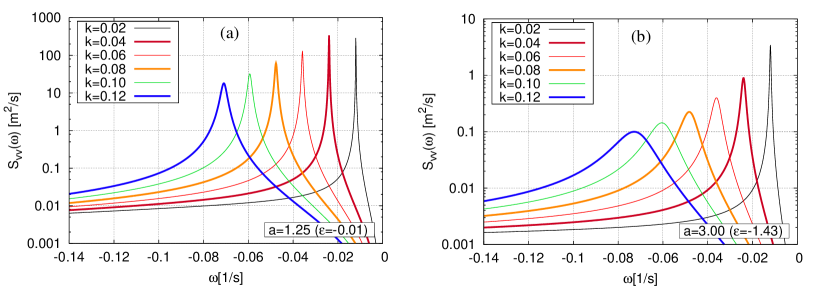
Fig. 3: Steady-state speed fluctuation spectrum for the control parameters $\epsilon=0.01$ (a) and $\epsilon=1.43$ (b). The IDM parameters, noise intensity, and the deterministic steady state is the same as in Figure 2.

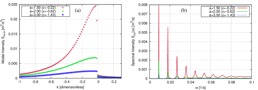
Fig. 4: (a) Modal speed fluctuation intensity for a ring road of length $L_{\rm ring}=10\,\mathrm{km}$ for three values of the relative proximity $\epsilon$ to the linear stability threshold. Each symbol denotes a possible mode $k=2n\pi/L_{\rm ring}$ (negative if propagating backwards). (b) Overall spectral intensity (14). The IDM parameters, noise intensity, and the deterministic steady state are the same as in Figure 2.

Fig. 5: Overall speed fluctuation intensity (15) as a function of the control parameter $\epsilon$ for the system of Figure 4.

Figure 3 confirms this observations for other order parameters. While it is expected that the spectral peaks become more pronounced very near the threshold ($\epsilon=-0.01$), significant peaks remain for $\epsilon=-1.43$, i.e., deep in the stable regime.

Figure 4 displays one-dimensional integrations of the modal speed fluctuation spectrum for a ring road of length $L_{\rm ring}=10\,000\,\mathrm{m}$. The panel (a) shows the modal fluctuation intensity

$$S_{uuk}=\int S_{uuk}(\omega)\ {\rm d}\omega$$ (13)

for some of the allowed modes near $k=0$. We observe that the integration eliminates the nontrivial peaks which is to be expected: After all, in the subcritical regime, the linear relaxation rate decreases with decreasing absolute values of the wavenumber thereby increasing, according to the fluctuation-dissipation theorem, the fluctuation intensities. Notice, however, that a distinct anisotropy favoring backwards propagating waves remain.

Panel 4(b) displays the overall spectral intensity

$$S_{uu}(\omega)=\sum_{k}S_{uuk}(\omega)$$ (14)

where the sum includes all allowed modes of the closed system. In contrast to plot4(a), distinct spectral peaks remain indicating resonances of the lowest allowed modes. The distance between the peaks is inversely proportional to the ring circumference.

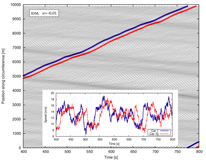
Fig. 6: Simulated IDM trajectories for a ring of 10 km circumference, $a=1.25\,\mathrm{m/s^{2}}$ ($\epsilon=-0.01$), and the remaining IDM parameters as in the main text. Every 3rd vehicle is shown. The inset shows speed time series of two selected vehicles.

Finally, Figure 5 displays the overall steady-state fluctuation intensity

$$S_{uu}=\sum_{k}\int S_{uuk}(\omega)\ {\rm d}\omega$$ (15)

of the speed of every single vehicle which is equal to the speed variance. Sufficiently far away from the threshold ($\epsilon<-0.2$), the variance is inversely proportional to $(-\epsilon)^{-1}$ corresponding to amplitudes proportional to $(-\epsilon)^{-0.5}$. Notice that the variance does not diverge at the linear stability limit which is caused (i) by finite-size effects, (ii) by nonlinear saturation. As expected, the speed fluctuation amplitude of a given vehicle is essentially independent of the system size.

In summary, the analytical investigation shows that the fluctuations triggered by white noise in the subcritical regime “anticipate” the characteristics of traffic waves in the collectively unstable regime. This is examplified in the simulated trajectories of Fig. 6 whose amplitude and spatiotemporal correlations agree quantitatively with the analytic theory. Moreover, the amplitude of the subcritical fluctuations increases strongly when approaching the linear threshold from below. The simulations in the following sections demonstrate that this can even lead to fully developed waves in the subcritical regime.

4 Vehicular Traffic: Platoon Experiments

In this section, we simulate platoon car-following experiments and test which of the three possible oscillation mechanisms, namely instability, noise, or action points, or which combinations thereof, allows for reproducing the empirical findings of a concave increase of the speed fluctuation amplitude as a function of the platoon vehicle number [25]). Moreover, by simulating these mechanisms with three underlying models (the IDM, the FVDM and the PCF model), we test to which extent the results are universal, i.e., independent of the specific car-following model. In the IDM and FVDM simulations, the white acceleration noise is integrated according to (2) resulting in fluctuations that are asymptotically independent of the simulation update time step [14]. The PCF model is simulated according to [19], i.e., realisations of the analytical distributions of the displacements are added to the locations in each time step which is set equal to its time-gap parameter $\tau=T=1\,\mathrm{s}$ (see below), so no discretisation errors incur.

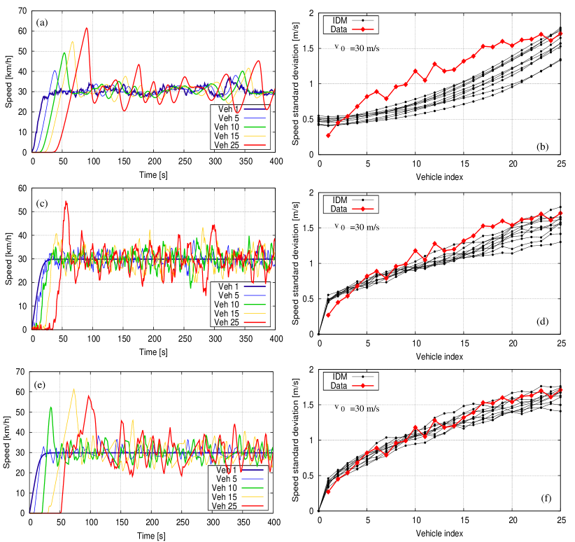
Fig. 7: Simulated speed time series (left column) and speed standard deviations (right column) for several vehicles in a platoon following the leader (Vehicle 1) accelerating slowly to the leading speed of 30 km/h. The simulation setup reproduces the platoon experiments of [26] (red symbols at the right column). In order to eliminate initial transients, the first 200 s of the simulation are skipped when calculating standard deviations. Top row: deterministic IDM far in the unstable regime ($a=0.5\,\mathrm{m/s^{2}}$ corresponding to $\epsilon=0.6$; some noise has been added to the leader to initiate oscillations); middle row: strong acceleration noise $Q=0.32\,\mathrm{m^{2}/s^{3}}$ at marginal stability ($\epsilon=0$) and without action points ($\Delta a_{\rm max}=0$); bottom row: only action points ($\Delta a_{\rm max}=1.2\,\mathrm{m/s^{2}}$, $Q=0$) at marginal stability. The remaining IDM parameters of the followers are given in the main text.

Figure 7 displays simulations of a platoon car-following experiment in China [26] (red symbols in the right column) where, in each row, only one of the three instability mechanisms is activated, namely string instability (top row), white acceleration noise (middle), and action points (bottom). Because of the stochastic nature, the detailed dynamics changes from run to run, so we show the growth of the speed standard deviation along the platoon for 10 realisations (right column). Additionally, we show in the left column the time series of a typical run. The leader drives fully deterministically (middle, bottom row) or with white noise (top row) according to the IDM and freely accelerates from speed zero at the begin of the experiments to a desired speed of $v_{0}^{\rm lead}=30\,\mathrm{km/h}$ corresponding to the experiment. The followers have a significantly higher desired speed and initially stand in a queue behind the leader. The IDM parameters of the followers that are not directly related to the oscillation mechanisms are set always to $v_{0}=108\,\mathrm{km/h}$, $T=1.0\,\mathrm{s}$, $s_{0}=2\,\mathrm{m}$, and $b=2\,\mathrm{m/s^{2}}$ (notice that the vehicle length is irrelevant in platoon simulations). The three oscillation mechanisms are controlled by the relative IDM acceleration $\epsilon=1-a/a_{c}$ (where $a_{c}=1.25\,\mathrm{m/s^{2}}$ for the above parameters and a leading speed of 30 km/h), $Q$ (noise intensity), and $\Delta a_{\rm max}$ (maximum acceleration change at an action point). In the simulations of each of the three mechanisms, the respective control parameter $\epsilon$, $Q$, and $\Delta a_{\rm max}$ has been calibrated to minimize the SSE between the observed and simulated speed standard deviations of all the vehicles (right column) over 10 simulation runs with independent seeds while the other two control parameters have been set to zero.

We find that the instability mechanism alone (Panels (a) and (b)) leads to oscillations that do not agree qualitatively with the platoon experiments. Notably, the increase of the fluctuation amplitude along the platoon vehicles is convex instead of concave. Furthermore, the calibrated IDM acceleration parameter $a=0.5\,\mathrm{m/s^{2}}$, or $\epsilon=0.6$, corresponds to an unrealistically unstable regime which leads to unrealistic results in simulation runs with longer platoons. Finally, the result depends sensitively on the noise intensity of the leading vehicle with no sensible results (no fluctuations) obtained for zero noise.

Panels 7(c) and (d) display the effect of external noise for a marginal stability $\epsilon=0$ and no action points, $\Delta a_{\rm max}=0$. In agreement with observations, we obtain a concave growth of the fluctuation amplitude along the platoon vehicles which, for $Q=0.32\,\mathrm{m^{2}/s^{3}}$, nearly quantitatively agrees with the experiment. Notice that the instability mechanism plays a role as well: The best results are obtained near marginal stability. Panels 7(e) and (f) give the results of simulations with active action points ($\Delta a_{\rm max}=1.2\,\mathrm{m/s^{2}}$) and deactivated noise ($Q=0$). Again, simulations near marginal stability ($\epsilon=0$) give the best results. Compared to the simulations with pure acceleration noise, the fit quality is even better. For most realisations, a good agreement is reached for the first platoon vehicles as well while the IDM with acceleration noise systematically overestimates the speed standard deviation of these vehicles.

We conclude that the instability mechanism alone is not able to reproduce the observations, even in the presence of a fluctuating leader. In contrast, both action points in the form of model (3) and white noise can reproduce the observations with best results obtained near marginal stability. Remarkably, action points and white noise are essentially interchangeable with action points giving marginally better results.

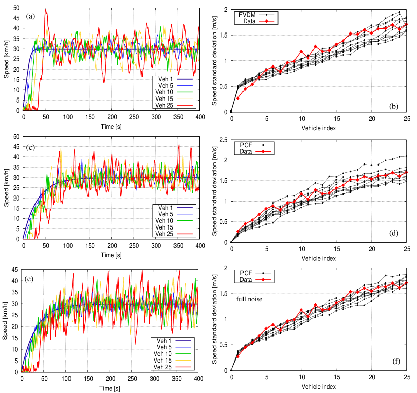
Fig. 8: Speed time series (left column) and speed standard deviations (right column) for the same initial configuration and the same leader’s speed profile as in Fig. 7. Top row: stochastic Full Velocity Difference Model (SFVDM) with a triangular fundamental diagram for calibrated model parameters; middle row: Parsimonious Car-Following Model (PCF model) [19] with the same fundamental diagram as the SFVDM. Bottom row: PCF model with the same parameters but stochasticity also turned on in the interacting regime. The values of the model parameters are given in the main text.

The question arises if these results depend on the underlying model, namely the IDM, or if other, possibly simpler, car-following models can be used as well. In order to test this proposition, we have performed simulations with the stochastic Full Velocity Difference Model (SFVDM) and also with the PCF model [19] of Laval et al which essentially implements the acceleration noise mechanism at marginal stability without interaction points. Instead of the optimal velocity (OV) function of the original FVDM [22], we apply an OV function corresponding to a tridiagonal fundamental diagram which resembles the IDM and has the same desired speed, desired time gap and minimum gap parameters. The resulting acceleration function of the FVDM reads

$$f(s,v,v_{l})=\beta\big{(}v_{\rm opt}(s)-v\big{)}+\lambda(v_{l}-v),\quad v_{\rm opt}(s)=\max\left(0,\min\left(v_{0},\frac{s-s_{0}}{T}\right)\right)$$ (16)

with values of the steady-state parameters $v_{0}=30\,\mathrm{m/s}$, $T=1.0\,\mathrm{s}$, and $s_{0}=2\,\mathrm{m}$ as in the IDM. We have chosen this particular OV function in order to reuse the steady-state IDM parameters, and also to compare the SFVDM with Newell’s car-following model [23] on which the PCF model is based and which has a tridiagonal fundamental diagram as well. Notice that, in the latter model, $T=\tau=1\,\mathrm{s}$ is associated not only with the time gap $T$ but also with the reaction delay time $\tau$ [8]; furthermore, the wave-speed parameter of this model can be identified by $w=(l_{\rm veh}+s_{0})/T$ where $l_{\rm veh}$ is the vehicle length which, however, does not play a role in the platoon simulations).

The top left panel of Fig. 8 shows an instance run of the SFVDM simulations with the calibrated dynamical parameters $1/\beta=10\,\mathrm{s}$, $\lambda=0.52\,\mathrm{s^{-1}}$, and the white-noise intensity $Q=0.25\,\mathrm{m^{2}/s^{3}}$. The top right panel displaying the speed standard deviations along the platoon for 10 realisations can be compared with that of the SIDM: Generally, we observe a good agreement. However, for most realisations, the simulated speed standard deviation of the first platoon vehicles is too high. Simulating the FVDM with action points (not shown) gives similar results as for the IDM.

The middle row gives a typical run for the PCF model with the recommended relaxation parameter $1/\beta=16\,\mathrm{s}$, and the calibrated noise intensity $Q=1.05\,\mathrm{m^{2}/s^{3}}$ (only for the followers) while the static parameters $v_{0}^{\rm lead}=8.3\,\mathrm{m/s}$, $v_{0}=30\,\mathrm{m/s}$, $T=\tau=1.0\,\mathrm{s}$, and $s_{0}=2\,\mathrm{m}$ are that of the other models. Notice that Ref. [19] recommends $1/\beta=16\,\mathrm{s}$ and a scaled noise intensity $\tilde{\sigma}^{2}=Q/(\beta v_{0}^{2})=0.11^{2}$ (Section 4) and $\tilde{\sigma}^{2}=0.15^{2}$ (Section 5). With $v_{0}=30\,\mathrm{m/s}$, this gives $Q=0.68\,\mathrm{m^{2}/s^{3}}$ and $Q=1.27\,\mathrm{m^{2}/s^{3}}$, respectively, which are of the same order of magnitude. (Notice that, for a given value of the scaled noise intensity, the physical noise intensity $Q$ depends strongly on the desired speed $v_{0}$ while only a weak dependency is plausible for the experiments.) Both values of the noise intensity are significantly higher as that calibrated for the stochastic IDM and FVDM. This is caused by the fact that the stochasticity of the PCF model is restricted to the free regime while, in the interacting regime (the speed is restricted by the leader), the PCF model reduces to Newell’s model, i.e., the drivers follow deterministically the leader’s trajectories with a constant space and time shift and, consequently, have the same constant variance as that of the leader. This applies whenever the realisation of the stochastic free displacement is greater than the deterministic displacement obtained from Newell’s model since the minimum of the displacements is taken in the model. The chance of deterministic car-following increases with decreasing $Q$, increasing $v_{0}$, and increasing $\beta$. For sufficiently low acceleration noise, this is always the case in our experiment and the PCF model reverts to deterministic car-following according to Newell’s model. This switching between a deterministic and a stochastic model seems also to be the reason why, although only implementing the acceleration noise mechanism, the PCF model fits the observations better than the SIDM and the SFVDM (and equally well as the IDM with action points): For the first platoon vehicles, the leaders exhibit only low-amplitude oscillations increasing the chance that the deterministic part of the PCF model applies. This reduces the effective acceleration noise of the first followers relative to that of the vehicles further behind thereby reducing the speed standard deviation of the first vehicles which is in line with the observation.

However, it is obviously unrealistic to switch from stochastic to deterministic driving when entering the car-following regime. Therefore, a straightforward generalization of the PCF model consists in adding the same acceleration noise to the car-following situation as well and also relax the rigid following rule of Newell’s model by introducing the same relaxation parameter $\beta$ as for the free part. It can be shown that the resulting “Full-noise PCF model” (FPCF model) is mathematically equivalent to (1) where $f$ is given by the time-delayed OVM with tridiagonal fundamental diagram,

$$f(s_{n}(t-T),v_{n}(t-T))=\beta\left(v_{\rm opt}(s(t-T))-v(t-T)\right),$$ (17)

with $v_{\rm opt}(s)$ given by FVDM. With the significantly reduced noise intensity $Q=0.2\,\mathrm{m^{2}/s^{3}}$, this model reproduces the data similarly well as the stochastic IDM and FVDM models which is to be expected since it utilizes the noise mechanism while having no action points and being at marginal stability (in Newell’s model, oscillations neither decay nor grow).

We conclude that the IDM is not necessary for our general findings and can be replaced by other underlying car-following models. In contrast, the mechanism matters. While the instability mechanism cannot reproduce the data even qualitatively, the action-point and noise mechanisms reproduce the data nearly quantitatively with the action-point mechanism and the selective-noise mechanism of the PCF model giving marginally better results than unconditional acceleration noise.

5 Bicycle Traffic on a Ring

The purpose of this section is twofold: Firstly, we demonstrate that, by a suitable change of the IDM parameters (particularly the vehicle length and the desired speed), the IDM can also be used to realistically simulate bicycle traffic. Secondly, we show that, for low-speed traffic, acceleration noise alone can lead to fully developed stop-and-go waves even in the subcritical regime.

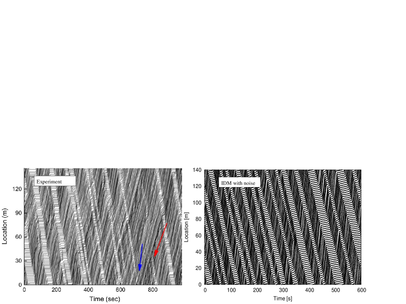
Fig. 9: Left: experimental trajectories of bicycles on a closed ring course of 140 m circumference; right: stochastic IDM simulation with acceleration noise $Q=0.4\,\mathrm{m^{2}/s^{3}}$. The IDM parameters corresponding to a subcritical situation are given in the main text.

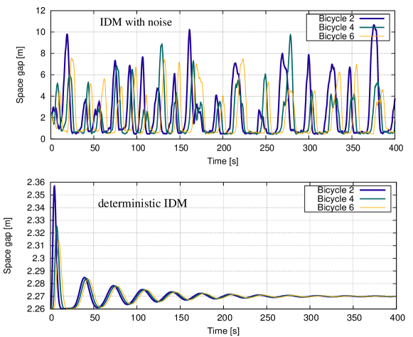
Fig. 10: Top panel: gap time series of the simulation of Fig. 9; bottom panel: time series for the deterministic simulation with zero acceleration noise, $Q=0$. The remaining parameters are that of Figure 9.

Figure 9 shows simulations (right) of bicycle experiments (left) on a ring road of 140 m circumference [27]. The bicycle length is assumed to be 1.67 m and the IDM parameters have been set to $v_{0}=4\,\mathrm{m/s}$, $T=0.6\,\mathrm{s}$, $s_{0}=0.4\,\mathrm{m}$, $a=0.8\,\mathrm{m/s^{2}}$, and $b=1.5\,\mathrm{m/s^{2}}$. A comparison of the simulated trajectories (right panel) with Fig. 3(c) of Ref. [27] (left panel) reveals a nearly quantitative agreement, at least in the statistical sense. The nearly triangular and symmetrical fundamental diagram (not shown) is consistent with the observations as well. Remarkably, the simulation is well in the subcritical regime ($\epsilon=-0.2$) which is mainly caused by the low speeds. Nevertheless, the acceleration noise alone ($Q=0.4\,\mathrm{m^{2}/s^{3}}$) leads to fully developed stop-and-go waves which can also be seen by the gap time series of selected bikers (Fig. 10, top panel). To validate this, we also run simulations without noise and unchanged parameters, otherwise (bottom panel). We observe that the initial transients quickly dissipate which is consistent with string stability.

6 Conclusion

In this contribution, we have proposed a minimal general model for simultaneously considering three possible mechanisms to traffic flow oscillations: string instability, external white acceleration noise, and indifference regions implemented by action points. Each of these mechanisms can be activated and controlled independently from the others by varying a single model parameter per mechanism, $\epsilon$, $Q$, and $\Delta a_{\rm max}$, respectively. The model is based on existing deterministic time-continuous car-following models with a fundamental diagram. However, the action-point mechanism introduces an indifference region and de facto converts this model into one consistent with the three-phase theory of Kerner [9].

By analytical means and numerical simulations, we have shown that white acceleration noise as well as the action points leads to highly spatiotemporally correlated fluctuations of speeds and gaps that “anticipate” the traffic waves produced by linear instabilities even well in the linearly stable region ($\epsilon<0$).

From the simulation results, we conclude that acceleration noise and action points lead to similar results. This means that the observed concave form of the fluctuation amplitude as a function of the vehicle index in a platoon can not only be reproduced by models of the three-phase theory, such as the 2D-IDM [28], but also by “two-phase models” such as the IDM when adding the simplest form of stochasticity, white (uncorrelated) acceleration noise.

We have also found that, for typical speeds of cars, acceleration noise and action points alone will not lead to realistic traffic oscillations. Additionally, at least marginal stability ($\epsilon=0$) or a mild form of linear instability ($\epsilon$ slightly positive) is necessary. In contrast, for low-speed traffic such as bicycle traffic, acceleration noise (or action points) alone can lead to fully developed and realistic traffic waves.

References

- [1] M. Mauch, M. J. Cassidy, Freeway traffic oscillations: observations and predictions, in: M. A. Taylor (Ed.), Transportation and traffic theory in the 21st century: Proceedings of the Symposium of Traffic and Transportation Theory, Elsevier, 2002, pp. 653–672.
- [2] S. Ahn, M. J. Cassidy, Freeway traffic oscillations and vehicle lane-change maneuvers, in: R. E. Allsop, M. G. H. Bell, B. G. Heydecker (Eds.), Transportation and Traffic Theory 2007, Elsevier, 2007, Ch. 29, pp. 691–710.
- [3] M. Schönhof, D. Helbing, Empirical features of congested traffic states and their implications for traffic modeling, Transportation Science 41 (2007) 1–32.
- [4] M. Treiber, A. Kesting, D. Helbing, Three-phase traffic theory and two-phase models with a fundamental diagram in the light of empirical stylized facts, Transportation Research Part B 44 (8-9) (2010) 983–1000.
- [5] B. Zielke, R. Bertini, M. Treiber, Empirical Measurement of Freeway Oscillation Characteristics: An International Comparison, Transportation Research Record 2088 (2008) 57–67.
- [6] R. Wilson, Mechanisms for spatio-temporal pattern formation in highway traffic models, Philosophical Transactions of the Royal Society A 366 (1872) (2008) 2017–2032.
- [7] G. Orosz, R. Wilson, R. Szalai, G. Stépán, Exciting traffic jams: Nonlinear phenomena behind traffic jam formation on highways, Physical Review E 80 (2009) 046205.
-
[8]
M. Treiber, A. Kesting, Traffic Flow Dynamics: Data, Models and Simulation,
Springer, Berlin, 2013.
URL http://www.traffic-flow-dynamics.org - [9] B. S. Kerner, The Physics of Traffic: Empirical Freeway Pattern Features, Engineering Applications, and Theory, Springer, 2012.
- [10] R. Jiang, M.-B. Hu, H. Zhang, Z.-Y. Gao, B. Jia, Q.-S. Wu, B. Wang, M. Yang, Traffic experiment reveals the nature of car-following, PloS one 9 (4) (2014) e94351.
- [11] R. Wiedemann, Simulation des Straßenverkehrsflußes, Vol. 8 of Schriftenreihe des IfV, Institut für Verkehrswesen, Universität Karlsruhe, 1974.
- [12] P. Wagner, I. Lubashevsky, Empirical basis for car-following theory development, preprint cond-mat/0311192.
- [13] A. Kesting, M. Treiber, How reaction time, update time and adaptation time influence the stability of traffic flow, Computer-Aided Civil and Infrastructure Engineering 23 (2008) 125–137.
- [14] M. Treiber, A. Kesting, D. Helbing, Delays, inaccuracies and anticipation in microscopic traffic models, Physica A 360 (2006) 71–88.
- [15] J. A. Laval, L. Leclercq, A mechanism to describe the formation and propagation of stop-and-go waves in congested freeway traffic, Philosophical Transactions of the Royal Society of London A: Mathematical, Physical and Engineering Sciences 368 (1928) (2010) 4519–4541.
- [16] H. Yeo, A. Skabardonis, Understanding stop-and-go traffic in view of asymmetric traffic theory, in: Transportation and Traffic Theory 2009: Golden Jubilee, Springer, 2009, pp. 99–115.
- [17] J. Tian, M. Treiber, S. Ma, B. Jia, W. Zhang, Microscopic driving theory with oscillatory congested states: Model and empirical verification, Transportation Research Part B: Methodological 71 (2015) 138–157.
- [18] M. Treiber, D. Helbing, Hamilton-like statistics in onedimensional driven dissipative many-particle systems, The European Physical Journal B 68 (2009) 607–618.
- [19] J. A. Laval, C. S. Toth, Y. Zhou, A parsimonious model for the formation of oscillations in car-following models, Transportation Research Part B: Methodological 70 (2014) 228–238.
- [20] J. A. Laval, L. Leclercq, Microscopic modeling of the relaxation phenomenon using a macroscopic lane-changing model, Transportation Research Part B: Methodological 42 (6) (2008) 511–522, newell’s CF model with bounded (deterministic accelerations.
- [21] M. Treiber, A. Hennecke, D. Helbing, Congested traffic states in empirical observations and microscopic simulations, Physical Review E 62 (2000) 1805–1824.
- [22] R. Jiang, Q. Wu, Z. Zhu, Full velocity difference model for a car-following theory, Physical Review E 64 (2001) 017101.
- [23] G. F. Newell, A simplified car-following theory: a lower order model, Transportation Research Part B: Methodological 36 (3) (2002) 195–205.
- [24] J. Honerkamp, Stochastic dynamical systems: concepts, numerical methods, data analysis, John Wiley & Sons, 1993.
- [25] J. Tian, R. Jiang, B. Jia, Z. Gao, S. Ma, Empirical analysis and simulation of the concave growth pattern of traffic oscillations, Transportation Research Part B: Methodological 93 (2016) 338–354.
-
[26]
J. Tian, G. Li, M. Treiber, R. Jiang, N. Jia, S. Ma, Cellular automaton model
simulating spatiotemporal patterns, phase transitions and concave growth
pattern of oscillations in traffic flow, Transportation Research Part B:
Methodological 93, Part A (2016) 560 – 575.
URL http://www.sciencedirect.com/science/article/pii/S0191261516305914 - [27] R. Jiang, M.-B. Hu, Q.-S. Wu, W.-G. Song, Traffic dynamics of bicycle flow: Experiment and modeling, Transportation Science.
- [28] J. Tian, R. Jiang, G. Li, M. Treiber, B. Jia, C. Zhu, Improved 2d intelligent driver model in the framework of three-phase traffic theory simulating synchronized flow and concave growth pattern of traffic oscillations, Transportation Research Part F: Traffic Psychology and Behaviour 41 (2016) 55–65.