A Hybrid Gyrokinetic Ion and Isothermal Electron Fluid Code for Astrophysical Plasma

Abstract

This paper describes a new code for simulating astrophysical plasmas that solves a hybrid model composed of gyrokinetic ions (GKI) and an isothermal electron fluid (ITEF) [A. Schekochihin et al., Astrophys. J. Suppl. 182, 310 (2009)]. This model captures ion kinetic effects that are important near the ion gyro-radius scale while electron kinetic effects are ordered out by an electron–ion mass ratio expansion. The code is developed by incorporating the ITEF approximation into AstroGK, an Eulerian $\delta f$ gyrokinetics code specialized to a slab geometry [R. Numata et al., J. Comput. Phys. 229, 9347 (2010)]. The new code treats the linear terms in the ITEF equations implicitly while the nonlinear terms are treated explicitly. We show linear and nonlinear benchmark tests to prove the validity and applicability of the simulation code. Since the fast electron timescale is eliminated by the mass ratio expansion, the Courant–Friedrichs–Lewy condition is much less restrictive than in full gyrokinetic codes; the present hybrid code runs $\sim 2\sqrt{m_{\mathrm{i}}/m_{\mathrm{e}}}\sim 100$ times faster than AstroGK with a single ion species and kinetic electrons where $m_{\mathrm{i}}/m_{\mathrm{e}}$ is the ion–electron mass ratio. The improvement of the computational time makes it feasible to execute ion scale gyrokinetic simulations with a high velocity space resolution and to run multiple simulations to determine the dependence of turbulent dynamics on parameters such as electron–ion temperature ratio and plasma beta.

1 Introduction

Understanding the thermodynamic properties of hot and dilute plasma is essential to advancing the study of astrophysics. This endeavor is particularly challenging because many astrophysical systems are in a weakly collisional state, where the collisional mean free path is comparable to or larger than the system size. Consequently, widely-used fluid models such as magnetohydrodynamics (MHD) are not suitable for describing the microscale physics that determine thermodynamic equilibrium. Instead, we need to treat the plasma using kinetic theory, in which the distribution of particle positions and velocities evolves in a six–dimensional phase space. The computational cost required to conduct such six-–dimensional (6D) computations is enormous: Even with the help of exascale computing, well-resolved 6D simulations are unlikely to be feasible in the near future.

Computational cost can be reduced significantly in magnetized plasma by adopting the gyrokinetic [1, 2, 3, 4, 5] model. A key ingredient of gyrokinetics is an assumed time scale separation created by the presence of a magnetic field; the ion cyclotron timescale is taken to be much faster than the timescale for the fluctuations of interest, i.e. $\Omega_{\mathrm{i}}\gg\omega$ with the ion cyclotron frequency $\Omega_{\mathrm{i}}$ and the fluctuation frequency $\omega$. This separation allows us to reduce the phase space from 6D to 5D — 3D in position space and 2D in velocity space — by averaging out the fast cyclotron motion. In the past few decades, gyrokinetics has been extensively used for studying microinstabilities and transport in magnetic confinement fusion devices [6, 7]. Recently, gyrokinetics has been highlighted as a powerful model in astrophysics as well [8, 9]. While many of the past astrophysical studies via gyrokinetics have targeted the solar wind [10, 11, 12, 13, 14, 15, 16, 17], gyrokinetics is also expected to be applicable to many other astrophysical objects, such as accretion flows, galaxy clusters, and interstellar media [9].

Although gyrokinetics improves the computational cost dramatically, it is still challenging to calculate 3D electromagnetic problems with high velocity space resolution. A further simplification to the gyrokinetic model can be made by carrying out an asymptotic expansion of the gyrokinetic-Maxwell system of equations in the smallness of the electron-ion mass ratio, $\sqrt{m_{\mathrm{e}}/m_{\mathrm{i}}}\sim 0.02$, with $m_{\mathrm{e}}$ and $m_{\mathrm{i}}$ the electron and proton masses, respectively. This limits the applicability of the model to spatial scales in the plane perpendicular to the mean magnetic field that are comparable to or larger than the ion Larmor radius. However, it also eliminates the fast time scale associated with the electron’s thermal speed and reduces the electron gyrokinetic equation to a set of fluid equations in which the electron temperature is constant along the mean magnetic field [18, 19, 9]. If one further assumes that the electron temperature does not vary across the mean magnetic field – as might be the case when the field is tangled – then one obtains the isothermal electron fluid (ITEF) model [9].

Coupling the ITEF with gyrokinetic ions (GKI) leads to a hybrid model that reduces computational cost by a factor of $\sim\sqrt{m_{\mathrm{e}}/m_{\mathrm{i}}}$ relative to full gyrokinetic model (FGK). While such a hybrid model with GKI and an ITEF has a long history in magnetic confinement fusion [34, 35, 36, 37, 38, 39, 40], it has not been applied to astrophysical plasmas. Moreover, unlike magnetic confinement fusion plasmas, many astrophysical plasmas have a plasma pressure comparable to and possibly much larger than the magnetic pressure; i.e., $\beta_{\mathrm{i}}=8\pi p_{\mathrm{i}}/B^{2}\sim 1-100$, with $p_{\mathrm{i}}$ the ion pressure and $B$ the magnetic field amplitude. This makes simulations rather cumbersome and increases the need for computational savings such as those provided by a hybrid code.

Therefore, it is valuable to develop a fluid–gyrokinetic hybrid code specialized for astrophysical studies. In this work, we develop a simulation code that solves the gyrokinetic ion and isothermal electron fluid (GKI/ITEF) equations [9] by implementing a new algorithm in AstroGK [41], a local, Eulerian, $\delta f$ gyrokinetics code developed for astrophysical studies. AstroGK [41] is based on the magnetic confinement fusion code GS2 [42, 43] but is optimized to treat plasmas with a straight, homogeneous mean magnetic field. Electrostatic simulations with AstroGK have been used to study the entropy cascade in phase space [44, 45, 46, 47], and electromagnetic simulations have been used to study magnetic reconnection [48, 49, 50, 51] in addition to the research on solar wind turbulence (reference listed above). To implement our hybrid model, we have modified the AstroGK algorithm to solve the ITEF equations coupled to the GKI-Maxwell’s system of equations. Since the most computationally intensive part of the hybrid code – the solution of the ion gyrokinetic equation – is unchanged, it retains the excellent parallel performance of AstroGK.

The outline of this paper is as follows. Section 2 presents a set of equations for the gyrokinetic model followed by the GKI/ITEF hybrid model. In Section 3, we describe the numerical algorithm for the hybrid code. We first briefly show the time integration algorithm adopted in AstroGK. We then show the detailed algorithm for solving the ITEF. In Section 4, we estimate the computational savings of the hybrid code relative to FGK codes. Section 5 presents the results of linear and nonlinear benchmark tests for code verification. It is found that the nonlinear test not only demonstrates the validity of the code but also reveals a non–trivial result which could be the starting point of a future study. In Section 6, we close with a summary of the paper.

2 Model equations

We start by presenting the FGK system of equations. Let us consider a homogeneous plasma immersed in magnetic field ${\boldsymbol{\mathrm{B}}}_{0}=B_{0}\hat{{\boldsymbol{\mathrm{z}}}}$. In astrophysical systems, ${\boldsymbol{\mathrm{B}}}_{0}$ may be assumed to be constant straight field at microscale. In $\delta f$ gyrokinetics, a particle distribution function $f_{s}$ for species $s$ is split into the mean and fluctuating parts:

$$f_{s}({\boldsymbol{\mathrm{r}}},{\boldsymbol{\mathrm{v}}},t)=F_{s}+\delta f_{s}=\left(1-\frac{q_{s}\phi({\boldsymbol{\mathrm{r}}})}{T_{s}}\right)F_{s}(v)+h_{s}(t,{\boldsymbol{\mathrm{R}}}_{s},v_{||},v_{\perp})$$ (1)

where $F_{s}=n_{s}(m_{s}/2\pi T_{s})^{3/2}\exp(-m_{s}v^{2}/2T_{s})$ is the mean distribution function assumed to be a Maxwellian with equilibrium density $n_{s}$ and temperature $T_{s}$, $\delta f_{s}$ is the fluctuating distribution function, $\phi$ is the fluctuating electrostatic potential, $h_{s}(t,{\boldsymbol{\mathrm{R}}}_{s},v_{||},v_{\perp})$ is the non-Boltzmann part of $\delta f_{s}$, ${\boldsymbol{\mathrm{R}}}_{s}={\boldsymbol{\mathrm{r}}}+{\boldsymbol{\mathrm{v}}}\times\hat{{\boldsymbol{\mathrm{z}}}}/\Omega_{s}$ is guiding center position, and ${||}$ ($\perp$) denotes the direction parallel (perpendicular) to $\hat{{\boldsymbol{\mathrm{z}}}}$. In the present study, we assume $n_{s}$ and $T_{s}$ are homogeneous in space. Electromagnetic (EM) fields are expressed in terms of the scalar and vector potentials, $\phi$ and ${\boldsymbol{\mathrm{A}}}$, as

$$\delta{\boldsymbol{\mathrm{B}}}=\nabla_{\perp}A_{||}\times\hat{{\boldsymbol{\mathrm{z}}}}+\delta B_{||}\hat{{\boldsymbol{\mathrm{z}}}},\quad{\boldsymbol{\mathrm{E}}}=-\nabla\phi-\frac{1}{c}\frac{\partial{\boldsymbol{\mathrm{A}}}}{\partial t}.$$ (2)

Substituting the forms for the distribution function and EM fields given by (1) and (2) into the Maxwell–Boltzmann system of equations and applying the gyrokinetic ordering, $\epsilon\sim k_{||}/k_{\perp}\sim\omega/\Omega_{s}\sim\delta f_{s}/F_{s}\sim\delta B/B_{0}$, we obtain the gyrokinetic equation [8]

$$\frac{\partial h_{s}}{\partial t}+v_{||}\frac{\partial h_{s}}{\partial z}+\frac{c}{B_{0}}\left\{\langle\chi\rangle_{{\boldsymbol{\mathrm{R}}}_{s}},h_{s}\right\}=\frac{q_{s}}{T_{s}}\frac{\partial\left<\chi\right>_{{\boldsymbol{\mathrm{R}}}_{s}}}{\partial t}F_{s}+\left<C[h_{s}]\right>_{{\boldsymbol{\mathrm{R}}}_{s}},$$ (3)

and Maxwell’s equations, viz., the quasi-neutrality condition, the parallel and perpendicular Ampere’s law,

$$\sum_{s}\frac{q_{s}^{2}n_{s}}{T_{s}}\phi=\sum_{s}q_{s}\int\mathrm{d}^{3}{\boldsymbol{\mathrm{v}}}\,\left<h_{s}\right>_{\boldsymbol{\mathrm{r}}},$$ (4a)

$$-\frac{c}{4\pi}\nabla_{\perp}^{2}A_{{||}}=\sum_{s}q_{s}\int\mathrm{d}^{3}{\boldsymbol{\mathrm{v}}}\,v_{||}\left<h_{s}\right>_{\boldsymbol{\mathrm{r}}},$$ (4b)

$$\frac{c}{4\pi}\nabla_{\perp}\delta B_{||}=\sum_{s}T_{s}\int\mathrm{d}^{3}{\boldsymbol{\mathrm{v}}}\,\left<(\hat{{\boldsymbol{\mathrm{z}}}}\times{\boldsymbol{\mathrm{v}}}_{\perp})h_{s}\right>_{\boldsymbol{\mathrm{r}}},$$ (4c)

where $\chi=\phi-{\boldsymbol{\mathrm{v}}}\cdot{\boldsymbol{\mathrm{A}}}/c$ is the gyrokinetic potential, $\left<\cdots\right>_{{\boldsymbol{\mathrm{R}}}_{s}}$ and $\left<\cdots\right>_{{\boldsymbol{\mathrm{r}}}}$ are the gyro–averages at fixed ${\boldsymbol{\mathrm{R}}}_{s}$ and ${\boldsymbol{\mathrm{r}}}$, respectively, $C[h_{s}]$ is a linearized collision operator that includes pitch angle scattering and energy diffusion satisfying conservation properties [52, 53], and $\left\{\cdots\,,\,\cdots\right\}$ is the Poisson bracket defined by

$$\left\{a,b\right\}=\hat{{\boldsymbol{\mathrm{z}}}}\cdot\frac{\partial a}{\partial{\boldsymbol{\mathrm{R}}}_{s}}\times\frac{\partial b}{\partial{\boldsymbol{\mathrm{R}}}_{s}}.$$ (5)

The assumed homogeneity of $F_{s}$ admits periodic solutions to these equations. We thus Fourier transform the fields in the plane perpendicular to $\hat{{\boldsymbol{\mathrm{z}}}}$:

$$h_{s}({\boldsymbol{\mathrm{R}}}_{s},v_{||},v_{\perp},t) =\sum_{{\boldsymbol{\mathrm{k}}}_{\perp}}h_{s{\boldsymbol{\mathrm{k}}}_{\perp}}(z,v_{||},v_{\perp},t)\,\mathrm{e}^{\mathrm{i}{\boldsymbol{\mathrm{k}}}_{\perp}\cdot{\boldsymbol{\mathrm{R}}}_{s}}$$ (6a)

$$\phi({\boldsymbol{\mathrm{r}}},t) =\sum_{{\boldsymbol{\mathrm{k}}}_{\perp}}\phi_{{\boldsymbol{\mathrm{k}}}_{\perp}}(z,t)\,\mathrm{e}^{\mathrm{i}{\boldsymbol{\mathrm{k}}}_{\perp}\cdot{\boldsymbol{\mathrm{r}}}}.$$ (6b)

The gyrokinetic equation in terms of Fourier component is

$$\frac{\partial g_{s{\boldsymbol{\mathrm{k}}}_{\perp}}}{\partial t}+v_{||}\frac{\partial g_{s{\boldsymbol{\mathrm{k}}}_{\perp}}}{\partial z}+v_{||}\frac{\partial}{\partial z}\left(J_{0}(a_{s})\frac{q_{s}\phi_{{\boldsymbol{\mathrm{k}}}_{\perp}}}{T_{s}}+\frac{2v_{\perp}^{2}}{v_{\mathrm{th}s}^{2}}\frac{J_{1}(a_{s})}{a_{s}}\frac{\delta B_{||{\boldsymbol{\mathrm{k}}}_{\perp}}}{B_{0}}\right)F_{s}+\frac{c}{B_{0}}\left\{\langle\chi\rangle_{{\boldsymbol{\mathrm{R}}}_{s}},h_{s}\right\}_{{\boldsymbol{\mathrm{k}}}_{\perp}}\\ =-\frac{q_{s}F_{s}}{T_{s}}\frac{v_{||}}{c}J_{0}(a_{s})\frac{\partial A_{||}}{\partial t}+C_{\mathrm{GK}}\left[h_{s{\boldsymbol{\mathrm{k}}}_{\perp}}\right],$$ (7)

where $g_{s{\boldsymbol{\mathrm{k}}}_{\perp}}$ is a complementary distribution function defined by

$$g_{s{\boldsymbol{\mathrm{k}}}}=h_{s{\boldsymbol{\mathrm{k}}}}-\frac{q_{s}F_{s}}{T_{s}}\left(J_{0}(a_{s})\phi_{{\boldsymbol{\mathrm{k}}}_{\perp}}+\frac{J_{1}(a_{s})}{a_{s}}\frac{2v_{\perp}^{2}}{v_{\mathrm{th}s}^{2}}\frac{T_{s}}{q_{s}}\frac{\delta B_{{||}{\boldsymbol{\mathrm{k}}}_{\perp}}}{B_{0}}\right),$$ (8)

$J_{n}(a_{s})$ is the Bessel function of the first kind with the argument $a_{s}=k_{\perp}v_{\perp}/\Omega_{s}$, $\left\{\cdots\,,\,\cdots\right\}_{{\boldsymbol{\mathrm{k}}}_{\perp}}$ is the Fourier transform of the Poisson bracket, $v_{\mathrm{th}s}=\sqrt{2T_{s}/m_{s}}$ is the thermal speed, and $C_{\mathrm{GK}}$ is the Fourier component of the gyro–averaged collision operator, i.e., $\left<C[h]\right>_{{\boldsymbol{\mathrm{R}}}_{s}}=\sum_{{\boldsymbol{\mathrm{k}}}_{\perp}}\mathrm{e}^{\mathrm{i}{\boldsymbol{\mathrm{R}}}_{s}\cdot{\boldsymbol{\mathrm{k}}}_{\perp}}C_{\mathrm{GK}}[h_{{\boldsymbol{\mathrm{k}}}_{\perp}}]$. Here the arguments of the Poisson bracket are evaluated in real space because we treat the nonlinear term by the pseudo-spectral method in the simulation code. The Fourier components of Maxwell’s equations are

$$\sum_{s}\frac{q_{s}^{2}n_{s}}{T_{s}}[1-\Gamma_{0}(\alpha_{s})]\phi_{{\boldsymbol{\mathrm{k}}}_{\perp}}-\sum_{s}q_{s}n_{s}\Gamma_{1}(\alpha_{s})\frac{\delta B_{||{\boldsymbol{\mathrm{k}}}_{\perp}}}{B_{0}}=\sum_{s}q_{s}\int\mathrm{d}^{3}{\boldsymbol{\mathrm{v}}}\,J_{0}(a_{s})g_{s{\boldsymbol{\mathrm{k}}}_{\perp}},$$ (9a)

$$\frac{ck_{\perp}^{2}}{4\pi}A_{{||}{\boldsymbol{\mathrm{k}}}_{\perp}}=\sum_{s}q_{s}\int\mathrm{d}^{3}{\boldsymbol{\mathrm{v}}}\,v_{||}J_{0}(a_{s})g_{s{\boldsymbol{\mathrm{k}}}_{\perp}},$$ (9b)

$$\frac{B_{0}}{4\pi}\delta B_{||{\boldsymbol{\mathrm{k}}}_{\perp}}+\sum_{s}q_{s}n_{s}\Gamma_{1}(\alpha_{s})\phi_{{\boldsymbol{\mathrm{k}}}_{\perp}}+\sum_{s}n_{s}T_{s}\Gamma_{2}(\alpha_{s})\frac{\delta B_{||{\boldsymbol{\mathrm{k}}}_{\perp}}}{B_{0}}=-\sum_{s}T_{s}\int\mathrm{d}^{3}{\boldsymbol{\mathrm{v}}}\,\frac{2v_{\perp}^{2}}{v_{\mathrm{th}s}^{2}}\frac{J_{1}(a_{s})}{a_{s}}g_{s{\boldsymbol{\mathrm{k}}}_{\perp}},$$ (9c)

where $\Gamma_{n}(\alpha_{s})$ is defined by

$$\Gamma_{0}(\alpha_{s})=I_{0}(\alpha_{s})\mathrm{e}^{-\alpha_{s}},\quad\Gamma_{1}(\alpha_{s})=[I_{0}(\alpha_{s})-I_{1}(\alpha_{s})]\mathrm{e}^{-\alpha_{s}},\quad\Gamma_{2}(\alpha_{s})=2\Gamma_{1}(\alpha_{s}),$$ (10)

with the $I_{n}$ modified Bessel functions of the first kind and $\alpha_{s}=k_{\perp}^{2}\rho_{s}^{2}/2$. AstroGK solves (7) and (9a)–(9c).

The GKI/ITEF equations are obtained by imposing two approximations to FGK, namely, massless electron ($\sqrt{m_{\mathrm{e}}/m_{\mathrm{i}}}\ll 1$) and isothermal electron closure ($\delta T_{\mathrm{e}}=0$) [9]. Expansion of (7) for electrons and (9a)–(9c) with respect to the small parameter $\sqrt{m_{\mathrm{e}}/m_{\mathrm{i}}}$ give a set of equations. One of the resulting equations, $\hat{{\boldsymbol{\mathrm{b}}}}\cdot\nabla\delta T_{\mathrm{e}}=0$ with the total magnetic field direction $\hat{{\boldsymbol{\mathrm{b}}}}=\hat{{\boldsymbol{\mathrm{z}}}}+\delta{\boldsymbol{\mathrm{B}}}_{\perp}/B_{0}$, restricts the electron temperature fluctuation along magnetic field line to be constant. We further assume that $\delta T_{\mathrm{e}}=$ constant, as would be the case if the magnetic field lines are tangled. By assuming $\delta T_{\mathrm{e}}=0$ (isothermal electron closure), the non–Boltzmann part of the perturbed electron distribution function is written by

$$h_{\mathrm{e}}^{(0)}=\left(\frac{\delta n_{\mathrm{e}}}{n_{\mathrm{e}}}-\frac{e}{T_{\mathrm{e}}}\phi\right)F_{\mathrm{e}},$$ (11)

where the superscript $(0)$ indicates zeroth order in $\sqrt{m_{\mathrm{e}}/m_{\mathrm{i}}}$. By substituting $h_{\mathrm{e}}^{(0)}$ to the electron gyrokinetic equation, one obtains the fluid dynamical equations for perturbed electron density $\delta n_{\mathrm{e}}$ and parallel electron flow speed $u_{{||}\mathrm{e}}$. In the resulting set of equations, the electron kinetic effects, which are primary effective at the electron gyro–radius scale, are neglected [9]. We consider a single ion species with charge $Ze$. The electron gyrokinetic equation is replaced by two dynamical equations:

$$\frac{\partial}{\partial t}\left(\frac{\delta n_{\mathrm{e}{\boldsymbol{\mathrm{k}}}_{\perp}}}{n_{\mathrm{e}}}-\frac{\delta B_{||{\boldsymbol{\mathrm{k}}}_{\perp}}}{B_{0}}\right)+\frac{c}{B_{0}}\left\{\phi-\frac{T_{\mathrm{e}}}{e}\frac{\delta n_{\mathrm{e}}}{n_{\mathrm{e}}},\,\frac{\delta n_{\mathrm{e}}}{n_{\mathrm{e}}}-\frac{\delta B_{||}}{B_{0}}\right\}_{{\boldsymbol{\mathrm{k}}}_{\perp}}+\frac{\partial u_{||\mathrm{e}{\boldsymbol{\mathrm{k}}}_{\perp}}}{\partial z}=\frac{1}{B_{0}}\{A_{||},\,u_{||\mathrm{e}}\}_{{\boldsymbol{\mathrm{k}}}_{\perp}},$$ (12a)

$$\frac{\partial A_{||{\boldsymbol{\mathrm{k}}}_{\perp}}}{\partial t}+\frac{c}{B_{0}}\left\{\phi-\frac{T_{\mathrm{e}}}{e}\frac{\delta n_{\mathrm{e}}}{n_{\mathrm{e}}},\,A_{||}\right\}_{{\boldsymbol{\mathrm{k}}}_{\perp}}+c\frac{\partial\phi_{{\boldsymbol{\mathrm{k}}}_{\perp}}}{\partial z}-\frac{cT_{\mathrm{e}}}{e}\frac{\partial}{\partial z}\left(\frac{\delta n_{\mathrm{e}{\boldsymbol{\mathrm{k}}}_{\perp}}}{n_{\mathrm{e}}}\right)=0,$$ (12b)

where the spatial gradient for the Poisson bracket is defined by the particle position ${\boldsymbol{\mathrm{r}}}$. The Maxwell’s equations (9a)–(9c) are rewritten as

$$\frac{\delta n_{\mathrm{e}{\boldsymbol{\mathrm{k}}}_{\perp}}}{n_{\mathrm{e}}}=\left[\Gamma_{0}(\alpha_{\mathrm{i}})-1\right]\frac{Ze\phi_{{\boldsymbol{\mathrm{k}}}_{\perp}}}{T_{\mathrm{i}}}+\Gamma_{1}(\alpha_{\mathrm{i}})\frac{\delta B_{{||}{\boldsymbol{\mathrm{k}}}_{\perp}}}{B_{0}}+\frac{1}{n_{\mathrm{i}}}\int\mathrm{d}^{3}{\boldsymbol{\mathrm{v}}}\,J_{0}(a_{\mathrm{i}})g_{\mathrm{i}{\boldsymbol{\mathrm{k}}}_{\perp}},$$ (13a)

$$u_{{||}\mathrm{e}{\boldsymbol{\mathrm{k}}}_{\perp}}=-\frac{ck_{\perp}^{2}}{4\pi en_{\mathrm{e}}}A_{{||}{\boldsymbol{\mathrm{k}}}_{\perp}}+\frac{1}{n_{\mathrm{i}}}\int\mathrm{d}^{3}{\boldsymbol{\mathrm{v}}}\,v_{||}J_{0}(a_{\mathrm{i}})g_{\mathrm{i}{\boldsymbol{\mathrm{k}}}_{\perp}},$$ (13b)

$$\frac{Z}{\tau}\frac{\delta n_{\mathrm{e}{\boldsymbol{\mathrm{k}}}_{\perp}}}{n_{\mathrm{e}}}+\left[\frac{2}{\beta_{\mathrm{i}}}+\Gamma_{2}(\alpha_{\mathrm{i}})\right]\frac{\delta B_{||{\boldsymbol{\mathrm{k}}}_{\perp}}}{B_{0}}=\left[1-\Gamma_{1}(\alpha_{\mathrm{i}})\right]\frac{Ze\phi_{{\boldsymbol{\mathrm{k}}}_{\perp}}}{T_{\mathrm{i}}}-\frac{1}{n_{\mathrm{i}}}\int\mathrm{d}^{3}{\boldsymbol{\mathrm{v}}}\,\frac{2v_{\perp}^{2}}{v_{\mathrm{thi}}^{2}}\frac{J_{1}(a_{\mathrm{i}})}{a_{\mathrm{i}}}g_{\mathrm{i}{\boldsymbol{\mathrm{k}}}_{\perp}},$$ (13c)

where $\tau=T_{\mathrm{i}}/T_{\mathrm{e}}$ and $\beta_{\mathrm{i}}=8\pi n_{\mathrm{i}}T_{\mathrm{i}}/B_{0}^{2}$.

Let us remark that the structure of the GKI/ITEF equations is altered from that of the FGK equations in the following sense. In FGK, the dynamical variables are ion and electron distribution functions, and EM fields are subsequently determined by Maxwell’s equation from the advanced distribution functions; in GKI/ITEF, $A_{||}$ is a dynamical variable, and $u_{{||}\mathrm{e}}$ is determined by the advanced $A_{||}$.

2.1 Generalized energy balance law

The generalized energy for the FGK system is defined as

$$W=\sum_{s}E_{f_{s}}+E_{B}=\sum_{s}\int\mathrm{d}^{3}{\boldsymbol{\mathrm{r}}}\int\mathrm{d}^{3}{\boldsymbol{\mathrm{v}}}\,\frac{T_{s}\delta f_{s}^{2}}{2F_{s}}+\int\mathrm{d}^{3}{\boldsymbol{\mathrm{r}}}\,\frac{|\delta{\boldsymbol{\mathrm{B}}}|^{2}}{8\pi}.$$ (14)

The energy balance law is given by [8, 9]

$$\frac{\mathrm{d}W}{\mathrm{d}t}=-\int\mathrm{d}^{3}{\boldsymbol{\mathrm{r}}}\,{\boldsymbol{\mathrm{J}}}_{a}\cdot{\boldsymbol{\mathrm{E}}}+\sum_{s}\int\mathrm{d}^{3}{\boldsymbol{\mathrm{R}}}_{s}\int\mathrm{d}^{3}{\boldsymbol{\mathrm{v}}}\,\frac{T_{s}}{F_{s}}\left<h_{s}C[h_{s}]\right>_{{\boldsymbol{\mathrm{R}}}_{s}},$$ (15)

where ${\boldsymbol{\mathrm{J}}}_{a}$ denotes external current drive (see Section 3.4) and the second term describes collisional entropy generation; thus $W$ is a constant of the motion in the absence of external power injection and collisions.

The generalized energy for the GKI/ITEF system is defined by [9]

$$W=E_{f_{\mathrm{i}}}+E_{n_{\mathrm{e}}}+E_{B}=\int\mathrm{d}^{3}{\boldsymbol{\mathrm{r}}}\int\mathrm{d}^{3}{\boldsymbol{\mathrm{v}}}\,\frac{T_{\mathrm{i}}\delta f_{\mathrm{i}}^{2}}{2F_{\mathrm{i}}}+\int\mathrm{d}^{3}{\boldsymbol{\mathrm{r}}}\,\frac{n_{\mathrm{e}}T_{\mathrm{e}}}{2}\frac{\delta n_{\mathrm{e}}^{2}}{n_{\mathrm{e}}}+\int\mathrm{d}^{3}{\boldsymbol{\mathrm{r}}}\,\frac{|\delta{\boldsymbol{\mathrm{B}}}|^{2}}{8\pi},$$ (16)

and its time rate of change obeys (15) with the electron collision ignored. When the system is 2D, i.e., $\partial_{z}=0$, there is an extra invariant for GKI/ITEF [9]:

$$I_{\mathrm{e}}=\int\mathrm{d}^{3}{\boldsymbol{\mathrm{r}}}\,\frac{A_{||}^{2}}{2}.$$ (17)

The conservation of these invariants is a good code verification, especially for a nonlinear run (Section 5.3).

2.2 Hyperviscosity for ITEF

As shown in Ref. [9], the energy that is cascaded from large scales is separated around the ion Larmor scale into ion entropy fluctuations and kinetic Alfvén waves (KAW). The energy in these two channels is independently cascaded to smaller scales, and then dissipated into thermal energy of ions and electrons respectively via collisions. In the GKI/ITEF hybrid model, the ion dissipation route exists, but the electron dissipation route is eliminated. Hence, an artificial dissipation mechanism is required to terminate the KAW cascade at the smallest scales. Such an artificial dissipation must (i) give a negative definite term in the right hand side of the energy balance equation (15) and (ii) be effective only at the smallest scales of the computational domain. We modify (12a) to include dissipation as follows:

$$\frac{\partial}{\partial t}\left(\frac{\delta n_{\mathrm{e}}}{n_{\mathrm{e}}}-\frac{\delta B_{||}}{B_{0}}\right)+\frac{c}{B_{0}}\left\{\phi-\frac{T_{\mathrm{e}}}{e}\frac{\delta n_{\mathrm{e}}}{n_{\mathrm{e}}},\,\frac{\delta n_{\mathrm{e}}}{n_{\mathrm{e}}}-\frac{\delta B_{||}}{B_{0}}\right\}+\frac{\partial u_{||\mathrm{e}}}{\partial z}=\frac{1}{B_{0}}\{A_{||},\,u_{||\mathrm{e}}\}+\nu_{h}\,\rho_{\mathrm{i}}^{2n}\nabla_{\perp}^{2n}\left(\frac{\delta n_{\mathrm{e}}}{n_{e}}-\frac{e}{T_{\mathrm{e}}}\phi\right).$$ (18)

The last term represents a hyperviscosity term where $\nu_{h}$ is the hyperviscosity coefficient and $n$ is a positive integer. This hyperviscosity term corresponds to the velocity integral of the collision operator acting on $h_{\mathrm{e}}^{(0)}$, which is estimated by (see Appendix B.1 in Ref. [9])

$$\frac{1}{n_{\mathrm{e}}}\int\mathrm{d}^{3}{\boldsymbol{\mathrm{v}}}\left<h_{\mathrm{e}}^{(0)}C[h_{\mathrm{e}}^{(0)}]\right>_{{\boldsymbol{\mathrm{R}}}_{\mathrm{e}}}\sim\sqrt{\frac{m_{\mathrm{e}}}{m_{\mathrm{i}}}}\nu_{\mathrm{i}\mathrm{i}}k_{\perp}^{2}\rho_{\mathrm{i}}^{2}\left(\frac{\delta n_{\mathrm{e}}}{n_{\mathrm{e}}}-\frac{e}{T_{\mathrm{e}}}\phi\right),$$ (19)

with the ion–ion collision frequency $\nu_{\mathrm{ii}}$. Whereas this should be ordered out as it is first order in $\sqrt{m_{\mathrm{e}}/m_{\mathrm{i}}}$, we can make it effective only at the small scales by changing $\sqrt{m_{\mathrm{e}}/m_{\mathrm{i}}}\nu_{\mathrm{ii}}k_{\perp}^{2}\rho_{\mathrm{i}}^{2}\to\nu_{h}k_{\perp}^{2n}\rho_{\mathrm{i}}^{2n}$. When the electrons have a Boltzmann response, i.e. $h_{\mathrm{e}}^{(0)}=0$, the hyperviscosity vanishes. This is consistent with the behavior of the exact Landau-Boltzmann collision operator, whose kernel includes the Maxwell-Boltzmann distribution. Using (18), the energy balance equation (15) is modified as

$$\frac{\mathrm{d}W}{\mathrm{d}t}=-\int\mathrm{d}^{3}{\boldsymbol{\mathrm{r}}}\,{\boldsymbol{\mathrm{J}}}_{a}\cdot{\boldsymbol{\mathrm{E}}}+\int\mathrm{d}^{3}{\boldsymbol{\mathrm{r}}}\int\mathrm{d}^{3}{\boldsymbol{\mathrm{v}}}\,\frac{T_{\mathrm{i}}}{F_{\mathrm{i}}}\left<h_{\mathrm{i}}C[h_{\mathrm{i}}]\right>_{{\boldsymbol{\mathrm{R}}}_{\mathrm{i}}}-\nu_{h}n_{\mathrm{e}}T_{\mathrm{e}}\int\mathrm{d}^{3}{\boldsymbol{\mathrm{r}}}\left|\rho_{\mathrm{i}}^{n}\nabla_{\perp}^{n}\left(\frac{\delta n_{\mathrm{e}}}{n_{\mathrm{e}}}-\frac{e}{T_{\mathrm{e}}}\phi\right)\right|^{2}.$$ (20)

Manifestly, the final term is negative definite.

We note that $A_{||}$ may not be damped by the hyperviscosity. However, we expect this would not cause a problem because the nonlinear term of $A_{||}$ evolution equation in $k_{\perp}\rho_{\mathrm{i}}\gg 1$ limit, which is proportional to $\{A_{||},\phi\}$ [9], is negligible when $\phi$ is sufficiently damped by the hyperviscosity. In fact, this has been confirmed by the 3D driven turbulence simulation [54]. On the other hand, $A_{||}$ can be directly damped by adding a term which is proportional to $-\nabla_{\perp}^{2n}u_{||\mathrm{e}}$ to the right hand side of (12b). This term plays a role of hyperresistivity. The new hybrid code does not have the hyperresistivity option at the moment as we have not found it necessary to attain converged results. However, it could be trivially implemented in the code if needed.

2.3 Normalization

We impose the same normalizations as those employed in AstroGK [41]

$$z=L_{||}\hat{z},\quad x=\rho_{0}\hat{x},\quad t=\frac{L_{||}}{v_{\mathrm{th0}}}\hat{t},\quad{\boldsymbol{\mathrm{v}}}=v_{\mathrm{th\mathrm{i}}}\hat{{\boldsymbol{\mathrm{v}}}}_{\mathrm{i}}=v_{\mathrm{th0}}\hat{v}_{\mathrm{thi}}\hat{{\boldsymbol{\mathrm{v}}}}_{\mathrm{i}},\quad m_{\mathrm{i}}=m_{0}\hat{m}_{\mathrm{i}},\quad$$

$$n_{\mathrm{i}}=n_{0}\hat{n}_{\mathrm{i}},\quad T_{\mathrm{i}}=T_{0}\hat{T}_{\mathrm{i}},\quad\beta_{\mathrm{i}}=\frac{8\pi n_{\mathrm{i}}T_{\mathrm{i}}}{B_{0}^{2}}=\hat{\beta}_{0}\hat{n}_{\mathrm{i}}\hat{T}_{\mathrm{i}},\quad$$

$$\delta n_{\mathrm{e}}=\frac{\rho_{0}}{L_{||}}n_{0}\widehat{\delta n}_{\mathrm{e}},\quad u_{{||}}=\frac{\rho_{0}}{L_{||}}v_{\mathrm{th}0}\hat{u}_{{||}},\quad\phi=\frac{\rho_{0}}{L_{||}}\frac{T_{0}}{e}\hat{\phi},\quad\delta B_{||}=\frac{\rho_{0}}{L_{||}}B_{0}\widehat{\delta B}_{||},\quad A_{||}=\frac{\rho_{0}}{L_{||}}\frac{cT_{0}}{v_{\mathrm{th0}}e}\hat{A}_{||},\quad$$

$$g_{\mathrm{i}}=\frac{\rho_{0}}{L_{||}}F_{\mathrm{i}}\hat{g}_{\mathrm{i}},\quad\frac{F_{\mathrm{i}}}{n_{\mathrm{i}}}\mathrm{d}^{3}{\boldsymbol{\mathrm{v}}}=\widehat{\mathrm{d}^{3}{\boldsymbol{\mathrm{v}}}}_{\mathrm{i}},\quad\nu_{h}=\left(\frac{1}{k_{\mathrm{max}}\rho_{\mathrm{i}}}\right)^{2n}\frac{v_{\mathrm{th0}}}{L_{||}}\hat{\nu}_{h}$$ (21)

where the subscripts 0 denote the reference values, $v_{\mathrm{th0}}=\sqrt{2T_{0}/m_{0}}$ is the reference thermal speed, $L_{||}$ is the parallel scale length, and $k_{\mathrm{max}}$ is the maximum perpendicular wave number. The resulting normalized GKI/ITEF equations are

$$\frac{\partial\hat{g}_{\mathrm{i}{\boldsymbol{\mathrm{k}}}_{\perp}}}{\partial\hat{t}}+\sqrt{\frac{\hat{T}_{\mathrm{i}}}{\hat{m}_{\mathrm{i}}}}\hat{v}_{{||}\mathrm{i}}\frac{\partial\hat{g}_{\mathrm{i}{\boldsymbol{\mathrm{k}}}_{\perp}}}{\partial\hat{z}}+\sqrt{\frac{\hat{T}_{\mathrm{i}}}{\hat{m}_{\mathrm{i}}}}\hat{v}_{{||}\mathrm{i}}\frac{\partial}{\partial\hat{z}}\left(J_{0}(\hat{a}_{\mathrm{i}})\frac{Z\hat{\phi}_{{\boldsymbol{\mathrm{k}}}_{\perp}}}{\hat{T}_{\mathrm{i}}}+2\hat{v}_{\perp\mathrm{i}}^{2}\frac{J_{1}(\hat{a}_{\mathrm{i}})}{\hat{a}_{\mathrm{i}}}\widehat{\delta B}_{||{\boldsymbol{\mathrm{k}}}_{\perp}}\right)+\frac{1}{2}\Big{\{}\langle\hat{\chi}\rangle_{{\boldsymbol{\mathrm{R}}}_{\mathrm{i}}},\hat{h}_{\mathrm{i}}\Big{\}}_{{\boldsymbol{\mathrm{k}}}_{\perp}}\\ =-\frac{Z}{\sqrt{\hat{m}_{\mathrm{i}}\hat{T}_{\mathrm{i}}}}\hat{v}_{{||}\mathrm{i}}J_{0}(\hat{a}_{\mathrm{i}})\frac{\partial\hat{A}_{||{\boldsymbol{\mathrm{k}}}_{\perp}}}{\partial\hat{t}}+C_{\mathrm{GK}}\left[\hat{h}_{\mathrm{i}{\boldsymbol{\mathrm{k}}}_{\perp}}\right],$$ (22)

$$\frac{\partial}{\partial\hat{t}}\left(\frac{\widehat{\delta n}_{\mathrm{e}{\boldsymbol{\mathrm{k}}}_{\perp}}}{\hat{n}_{\mathrm{e}}}-\widehat{\delta B}_{||{\boldsymbol{\mathrm{k}}}_{\perp}}\right)+\frac{1}{2}\Bigg{\{}\hat{\phi}-\frac{\hat{T}_{\mathrm{i}}}{\tau}\frac{\widehat{\delta n}_{\mathrm{e}}}{\hat{n}_{\mathrm{e}}},\,\frac{\widehat{\delta n}_{\mathrm{e}}}{\hat{n}_{\mathrm{e}}}-\widehat{\delta B}_{||{\boldsymbol{\mathrm{k}}}_{\perp}}\Bigg{\}}_{{\boldsymbol{\mathrm{k}}}_{\perp}}+\frac{\partial\hat{u}_{||\mathrm{e}{\boldsymbol{\mathrm{k}}}_{\perp}}}{\partial\hat{z}}\\ =\frac{1}{2}\big{\{}\hat{A}_{||},\,\hat{u}_{||\mathrm{e}}\big{\}}_{{\boldsymbol{\mathrm{k}}}_{\perp}}-\hat{\nu}_{h}\left(\frac{\hat{k}_{\perp}}{\hat{k}_{\mathrm{max}}}\right)^{2n}\left(\frac{\widehat{\delta n}_{\mathrm{e}{\boldsymbol{\mathrm{k}}}_{\perp}}}{\hat{n}_{\mathrm{e}}}-\frac{\tau}{\hat{T}_{\mathrm{i}}}\hat{\phi}_{{\boldsymbol{\mathrm{k}}}_{\perp}}\right),$$ (23a)

$$\frac{\partial\hat{A}_{||{\boldsymbol{\mathrm{k}}}_{\perp}}}{\partial\hat{t}}+\frac{1}{2}\left\{\hat{\phi}-\frac{\hat{T}_{\mathrm{i}}}{\tau}\frac{\widehat{\delta n}_{\mathrm{e}}}{\hat{n}_{\mathrm{e}}},\,\hat{A}_{||}\right\}_{{\boldsymbol{\mathrm{k}}}_{\perp}}+\frac{\partial\hat{\phi}_{{\boldsymbol{\mathrm{k}}}_{\perp}}}{\partial\hat{z}}-\frac{\hat{T}_{\mathrm{i}}}{\tau}\frac{\partial}{\partial\hat{z}}\left(\frac{\widehat{\delta n}_{\mathrm{e}{\boldsymbol{\mathrm{k}}}_{\perp}}}{\hat{n}_{\mathrm{e}}}\right)=0,$$ (23b)

$$\frac{\widehat{\delta n}_{\mathrm{e}{\boldsymbol{\mathrm{k}}}_{\perp}}}{\hat{n}_{\mathrm{e}}}=\left[\Gamma_{0}(\hat{\alpha}_{\mathrm{i}})-1\right]\frac{Z\hat{\phi}_{{\boldsymbol{\mathrm{k}}}_{\perp}}}{\hat{T}_{\mathrm{i}}}+\Gamma_{1}(\hat{\alpha}_{\mathrm{i}})\delta B_{{||}{\boldsymbol{\mathrm{k}}}_{\perp}}+\int\widehat{\mathrm{d}^{3}{\boldsymbol{\mathrm{v}}}}_{\mathrm{i}}\,J_{0}(\hat{a}_{\mathrm{i}})\hat{g}_{\mathrm{i}{\boldsymbol{\mathrm{k}}}_{\perp}}$$ (24a)

$$\hat{u}_{{||}\mathrm{e}{\boldsymbol{\mathrm{k}}}_{\perp}}=-\frac{\hat{k}_{\perp}^{2}\hat{A}_{{||}{\boldsymbol{\mathrm{k}}}_{\perp}}}{2\beta_{0}Z\hat{n}_{\mathrm{i}}}+\sqrt{\frac{\hat{T}_{\mathrm{i}}}{\hat{m}_{\mathrm{i}}}}\int\widehat{\mathrm{d}^{3}{\boldsymbol{\mathrm{v}}}}_{\mathrm{i}}\,\hat{v}_{{||}\mathrm{i}}J_{0}(\hat{a}_{\mathrm{i}})\hat{g}_{\mathrm{i}{\boldsymbol{\mathrm{k}}}_{\perp}},$$ (24b)

$$\frac{Z}{\tau}\frac{\widehat{\delta n}_{\mathrm{e}{\boldsymbol{\mathrm{k}}}_{\perp}}}{\hat{n}_{\mathrm{e}}}+\left[\frac{2}{\hat{\beta}_{0}\hat{n}_{\mathrm{i}}\hat{T}_{\mathrm{i}}}+\Gamma_{2}(\hat{\alpha}_{\mathrm{i}})\right]\widehat{\delta B}_{||{\boldsymbol{\mathrm{k}}}_{\perp}}=\left[1-\Gamma_{1}(\hat{\alpha}_{\mathrm{i}})\right]\frac{Z\hat{\phi}_{{\boldsymbol{\mathrm{k}}}_{\perp}}}{\hat{T}_{\mathrm{i}}}-\int\widehat{\mathrm{d}^{3}{\boldsymbol{\mathrm{v}}}}_{\mathrm{i}}\,2\hat{v}_{\perp\mathrm{i}}^{2}\frac{J_{1}(\hat{a}_{\mathrm{i}})}{\hat{a}_{\mathrm{i}}}\hat{g}_{\mathrm{i}{\boldsymbol{\mathrm{k}}}_{\perp}}.$$ (24c)

where

$$\hat{a}_{\mathrm{i}}=\sqrt{\hat{m}_{\mathrm{i}}\hat{T}_{\mathrm{i}}}\frac{\hat{k}_{\perp}\hat{v}_{\perp\mathrm{i}}}{Z},\quad\hat{\alpha}_{\mathrm{i}}=\frac{\hat{m}_{\mathrm{i}}\hat{T}_{\mathrm{i}}}{Z^{2}}\frac{\hat{k}_{\perp}^{2}}{2}.$$ (25)

Henceforth, we omit the hat symbols in order to simplify notation.

3 Numerical Algorithm

In this section, we describe the numerical algorithm used to solve the GKI/ITEF equations (22), (23a)–(23b), and (24a)–(24c). We start by providing a brief overview of the algorithm used in AstroGK for solving the FGK equations (detailed in Ref. [41]) before detailing the modifications we made to solve the GKI/ITEF equations.

3.1 Implicit time advance for FGK linear terms

In AstroGK, the linear terms in the gyrokinetic equation (7) is solved implicitly together with Maxwell’s equations (9a)–(9c) via a Green’s function approach [42]. For the linear terms, we employ a Fourier-spectral method in the perpendicular plane, ($x,y$), and a compact finite-difference method to evaluate a derivative in parallel direction, $\partial_{z}$. The nonlinear terms is treated by pseudo-spectral method (see Section 3.3). Since there is no explicit perpendicular derivative, $\partial_{x}$ and $\partial_{y}$, except for the nonlinear terms, all the equations are independent with respect to the Fourier modes. The velocity space is spanned by three variables, pitch angle $\lambda=v_{\perp}^{2}/v^{2}$, energy $E=v_{\perp}^{2}+v_{||}^{2}$, and the sign of the parallel velocity $\sigma=\mathrm{sgn}(v_{||})$. Below, we omit the species index $s$ since it is unnecessary here. Let us denote the discretized fields by

$$g_{\mathrm{i}{\boldsymbol{\mathrm{k}}}_{\perp}}=g^{n}_{i,p,q},\quad\frac{\delta n_{\mathrm{e}{\boldsymbol{\mathrm{k}}}_{\perp}}}{n_{\mathrm{e}}}=\eta^{n}_{i},\quad u_{||\mathrm{e}{\boldsymbol{\mathrm{k}}}_{\perp}}={u_{||}}^{n}_{i},\quad\phi_{{\boldsymbol{\mathrm{k}}}_{\perp}}=\phi^{n}_{i},\quad A_{||{\boldsymbol{\mathrm{k}}}_{\perp}}={A_{||}}^{n}_{i},\quad\delta B_{||{\boldsymbol{\mathrm{k}}}_{\perp}}={B_{||}}^{n}_{i}.$$ (26)

with the indices corresponding to time grids $t_{n}=\sum_{j=1}^{n}\Delta t_{j}\;(n=1,\cdots,n_{t})$, parallel space grids $z_{i}=i\Delta z\;(i=1,\cdots,n_{z})$, and velocity space grids $E_{p}\,(p=1,\cdots,n_{E})$ and $\lambda_{q}\,(q=1,\cdots,n_{\lambda})$. The index for $\sigma$ is omitted. Here $\Delta t_{j}$ is an adaptive timestep which is modified when the advection speed violates the Courant–Friedrichs–Lewy (CFL) condition [55] or considerably larger than the maximum timestep determined by the CFL condition (see Section 3.3). Allowing temporal and spatial implicitness by parameters $r_{t}$ and $r_{z}$, the derivatives with respect to $t$ and $z$ are evaluated by

$$\frac{\partial f}{\partial t}=\frac{1}{2}\left[(1-r_{z})\frac{f^{n+1}_{i}-f^{n}_{i}}{\Delta t}+(1+r_{z})\frac{f^{n+1}_{i+1}-f^{n}_{i+1}}{\Delta t}\right]\quad\text{and}\quad\frac{\partial f}{\partial z}=r_{t}\frac{f^{n}_{i+1}-f^{n}_{i}}{\Delta z}+(1-r_{t})\frac{f^{n+1}_{i+1}-f^{n+1}_{i}}{\Delta z},$$ (27)

where $0<r_{t}<1$ ($r_{t}=0$ for fully implicit and $r_{t}=1$ for fully explicit) and $0<r_{z}<1$ ($r_{z}=0$ for central difference and $r_{z}=1$ for first order upwind difference). Especially when $r_{t}=1/2$ and $r_{z}=0$, i.e., space and time centered [56], the scheme has second order accuracy both in space and time, and unconditionally stable.

The discretization of (7) may be written symbolically as,

$$a_{1}g^{n}_{j}+a_{2}g^{n}_{j+1}+b_{1}g^{n+1}_{j}+b_{2}g^{n+1}_{j+1}={\boldsymbol{\mathrm{c}}}_{1}\cdot{\boldsymbol{\mathrm{\Psi}}}^{n}_{j}+{\boldsymbol{\mathrm{c}}}_{2}\cdot{\boldsymbol{\mathrm{\Psi}}}^{n}_{j+1}+{\boldsymbol{\mathrm{d}}}_{1}\cdot{\boldsymbol{\mathrm{\Psi}}}^{n+1}_{j}+{\boldsymbol{\mathrm{d}}}_{2}\cdot{\boldsymbol{\mathrm{\Psi}}}^{n+1}_{j+1}+\mathcal{N}_{j}+\mathcal{N}_{j+1},$$ (28)

where ${\boldsymbol{\mathrm{\Psi}}}=(\phi,A_{||},B_{||})$, the coefficients depend on Fourier space (${\boldsymbol{\mathrm{k}}}_{\perp}$) and velocity space ($\lambda$ and $E$), $\mathcal{N}$ represents the nonlinear term, and the velocity space indices $(p,q)$ are omitted. Maxwell’s equations (9a)–(9c) are compactly written as

$$\mathsf{M}\cdot{\boldsymbol{\mathrm{\Psi}}}^{n+1}_{i}=\sum_{p}\sum_{q}{\boldsymbol{\mathrm{f}}}_{p,q}\,g^{n+1}_{i,p,q},$$ (29)

where $\mathsf{M}$ is a block $3\times 3$ matrix with each block as $n_{z}\times n_{z}$ submatrix, and the right hand side represents the velocity space integrals appearing in (24a)–(24c). We note that $\mathsf{M}$ and ${\boldsymbol{\mathrm{f}}}$ depend neither on $t$ nor $z$. One may straightforwardly obtain $g^{n+1}$ by substituting (29) into (28). However, such a brute force method is not practical since it requires an inversion of a dense $(n_{z}n_{\lambda}n_{E}n_{\sigma}n_{s})^{2}$ size matrix.

Kotschenreuther et al. found that the linear property of the equation enables us to break this large matrix into many small matrices [42], and by doing so, computational efficiency dramatically improves (see [41] for the detailed estimate). Since (28) is linear in $g^{n+1}$, its solution is a linear combination of solutions to parts of the equation. We split the distribution function at timestep $n+1$ into homogeneous and inhomogeneous parts, viz. $g^{n+1}=g^{\mathrm{(h)}}+g^{\mathrm{(inh)}}$ and introduce an intermediate timestep variable of EM fields, ${\boldsymbol{\mathrm{\Psi}}}^{*}={\boldsymbol{\mathrm{\Psi}}}^{n+1}-{\boldsymbol{\mathrm{\Psi}}}^{n}$. Then (28) is split into

$$a_{1}g^{n}_{j}+a_{2}g^{n}_{j+1}+b_{1}g^{\mathrm{(inh)}}_{j}+b_{2}g^{\mathrm{(inh)}}_{j+1}={\boldsymbol{\mathrm{c}}}_{1}\cdot{\boldsymbol{\mathrm{\Psi}}}^{n}_{j}+{\boldsymbol{\mathrm{c}}}_{2}\cdot{\boldsymbol{\mathrm{\Psi}}}^{n}_{j+1}+{\boldsymbol{\mathrm{d}}}_{1}\cdot{\boldsymbol{\mathrm{\Psi}}}^{n}_{j}+{\boldsymbol{\mathrm{d}}}_{2}\cdot{\boldsymbol{\mathrm{\Psi}}}^{n}_{j+1}+\mathcal{N}_{j}+\mathcal{N}_{j+1},$$ (30a)

$$b_{1}g^{\mathrm{(h)}}_{j}+b_{2}g^{\mathrm{(h)}}_{j+1}={\boldsymbol{\mathrm{d}}}_{1}\cdot{\boldsymbol{\mathrm{\Psi}}}^{*}_{j}+{\boldsymbol{\mathrm{d}}}_{2}\cdot{\boldsymbol{\mathrm{\Psi}}}^{*}_{j+1}.$$ (30b)

Now, $g^{\mathrm{(inh)}}_{i}$ is immediately obtained by solving (30a). We formally rewrite (30b) as

$$g^{(\mathrm{h})}_{i,p,q}({\boldsymbol{\mathrm{\Psi}}}^{*})=\sum_{j}\left(\frac{\delta g}{\delta{\boldsymbol{\mathrm{\Psi}}}}\right)_{ijpq}\cdot{\boldsymbol{\mathrm{\Psi}}}^{*}_{j},$$ (31)

where $(\delta g/\delta{\boldsymbol{\mathrm{\Psi}}})_{ijpq}$ is a so-called response matrix which is obtained by the following procedure. For a given integer $l$, we substitute trial functions $\phi^{*}_{j}=\delta_{jl}$, ${A_{||}}^{*}_{j}=0$, and ${B_{||}}^{*}_{j}=0$ with the Kronecker’s delta $\delta_{ij}$ into (30b) and solve it for $g^{\mathrm{(h)}}_{j,p,q}$. Then the obtained $g^{\mathrm{(h)}}_{j,p,q}$ is equivalent to $(\delta g/\delta\phi)_{jlpq}$. Recursion of this process over $l=1,\cdots,n_{z}$ yields the complete set of $(\delta g/\delta\phi)_{jlpq}$. The other components of the response matrix, $(\delta g/\delta A_{||})$ and $(\delta g/B_{||})$, are obtained by using the trial functions in the same way for ${A_{||}}^{*}_{j}$ and ${B_{||}}^{*}_{j}$. Substituting (31) into (29) and moving the terms including ${\boldsymbol{\mathrm{\Psi}}}^{*}$ to the left hand side and the others to the right hand side, we get

$$\left[\mathsf{M}\delta_{ij}-\sum_{p}\sum_{q}{\boldsymbol{\mathrm{f}}}_{p,q}\sum_{j}\left(\frac{\delta g}{\delta{\boldsymbol{\mathrm{\Psi}}}}\right)_{ijpq}\right]\cdot{\boldsymbol{\mathrm{\Psi}}}^{*}_{j}=-\mathsf{M}\cdot{\boldsymbol{\mathrm{\Psi}}}^{n}_{i}+\sum_{p}\sum_{q}{\boldsymbol{\mathrm{f}}}_{p,q}\,g^{\mathrm{(inh)}}_{i,p,q}.$$ (32)

We obtain ${\boldsymbol{\mathrm{\Psi}}}^{*}$ by inversion of the coefficient matrix. Successively $g^{n+1}$ is obtained by (28). We calculate the coefficient matrix in the initialization step and keep using it unless $\Delta t$ is modified by the CFL condition (see Section 3.3).

3.2 Time integration algorithm for the hybrid code

Next we consider the time advance algorithm for (22), (23a)–(23b) and (24a)–(24c). Using the finite difference (27), we discretize (23a) and (23b) as

$$\frac{1}{2}\left[(1-r_{z})\frac{\eta^{n+1}_{i}-\eta^{n}_{i}}{\Delta t}+(1+r_{z})\frac{\eta^{n+1}_{i+1}-\eta^{n}_{i+1}}{\Delta t}\right]-\frac{1}{2}\left[(1-r_{z})\frac{{B_{||}}^{n+1}_{i}-{B_{||}}^{n}_{i}}{\Delta t}+(1+r_{z})\frac{{B_{||}}^{n+1}_{i+1}-{B_{||}}^{n}_{i+1}}{\Delta t}\right]\\ +r_{t}\frac{{u_{||}}^{n}_{i+1}-{u_{||}}^{n}_{i}}{\Delta z}+(1-r_{t})\frac{{u_{||}}^{n+1}_{i+1}-{u_{||}}^{n+1}_{i}}{\Delta z}=-\frac{\nu_{h}}{4}\left(\frac{k_{\perp}}{k_{\mathrm{max}}}\right)^{2n}\Bigg{\{}\left[(1-r_{z})\left(\eta^{n+1}_{i}+\eta^{n}_{i}\right)+(1+r_{z})\left(\eta^{n+1}_{i+1}+\eta^{n}_{i+1}\right)\right]\\ -\frac{\tau}{T_{0\mathrm{i}}}\left[(1-r_{z})\left(\phi^{n+1}_{i}+\phi^{n}_{i}\right)+(1+r_{z})\left(\phi^{n+1}_{i+1}+\phi^{n}_{i+1}\right)\right]\Bigg{\}}+\frac{1}{2}\left[(1+r_{z})\mathcal{N}^{(\eta)}_{i+1}+(1-r_{z})\mathcal{N}^{(\eta)}_{i}\right]$$ (33)

$$\frac{1}{2}\left[(1-r_{z})\frac{{A_{||}}^{n+1}_{i}-{A_{||}}^{n}_{i}}{\Delta t}+(1+r_{z})\frac{{A_{||}}^{n+1}_{i+1}-{A_{||}}^{n}_{i+1}}{\Delta t}\right]+r_{t}\frac{\phi^{n}_{i+1}-\phi^{n}_{i}}{\Delta z}+(1-r_{t})\frac{\phi^{n+1}_{i+1}-\phi^{n+1}_{i}}{\Delta z}\\ =\frac{T_{\mathrm{i}}}{\tau}\left[r_{t}\frac{\eta^{n}_{i+1}-\eta^{n}_{i}}{\Delta z}+(1-r_{t})\frac{\eta^{n+1}_{i+1}-\eta^{n+1}_{i}}{\Delta z}\right]+\frac{1}{2}\left[(1+r_{z})\mathcal{N}^{(A_{||})}_{i+1}+(1-r_{z})\mathcal{N}^{(A_{||})}_{i}\right]$$ (34)

We may choose the value of $r_{t}$ and $r_{z}$ independently from the ion gyrokinetic equation (22). The Maxwell’s equations (24a)–(24c) are discretized as

$$Zn_{\mathrm{i}}\eta^{n+1}_{i}=-\mathpzc{G}_{0}\phi^{n+1}_{i}+\mathpzc{G}_{1}{B_{||}}^{n+1}_{i}+\mathcal{M}^{(0)}\left(g^{n+1}_{i}\right)$$ (35a)

$$2\beta_{0}Zn_{\mathrm{i}}{u_{||}}^{n+1}_{i}=-k_{\perp}^{2}{A_{||}}^{n+1}_{i}+\mathcal{M}^{(1)}\left(g^{n+1}_{i}\right)$$ (35b)

$$\frac{n_{\mathrm{i}}T_{\mathrm{i}}Z}{2\tau}{\eta}^{n+1}_{i}+\left(\frac{1}{\beta_{0}}+\mathpzc{G}_{2}\right){B_{||}}^{n+1}_{i}=\frac{1}{2}\left(n_{\mathrm{i}}Z-\mathpzc{G}_{1}\right){\phi}^{n+1}_{i}-\mathcal{M}^{(2)}\left(g^{n+1}_{i}\right)$$ (35c)

Here the coefficients are defined by

$$\mathpzc{G}_{0}=\frac{Z^{2}n_{\mathrm{i}}}{T_{\mathrm{i}}}\left[1-\Gamma_{0}(\alpha_{\mathrm{i}})\right],\quad\mathpzc{G}_{1}=Zn_{\mathrm{i}}\Gamma_{1}(\alpha_{\mathrm{i}}),\quad\mathpzc{G}_{2}=\frac{1}{2}n_{\mathrm{i}}T_{\mathrm{i}}\Gamma_{2}(\alpha_{\mathrm{i}}),$$ (36)

the nonlinear terms are represented by

$$\mathcal{N}^{(A_{||})}=-\frac{1}{2}\Big{\{}\phi-\frac{T_{\mathrm{i}}}{\tau}\eta,\,A_{||}\Big{\}}$$ (37a)

$$\mathcal{N}^{(\eta)}=-\frac{1}{2}\Big{\{}\phi-\frac{T_{\mathrm{i}}}{\tau}\eta,\,\eta-\delta B_{||{\boldsymbol{\mathrm{k}}}_{\perp}}\Big{\}}+\frac{1}{2}\Big{\{}A_{||},\,u_{||\mathrm{e}}\Big{\}},$$ (37b)

and the velocity integral operators are defined by

$$\mathcal{M}^{(0)}\left(g_{\mathrm{i}{\boldsymbol{\mathrm{k}}}_{\perp}}\right)=n_{\mathrm{i}}Z\int\mathrm{d}^{3}{\boldsymbol{\mathrm{v}}}_{\mathrm{i}}\,J_{0}(a_{\mathrm{i}})g_{\mathrm{i}{\boldsymbol{\mathrm{k}}}_{\perp}}$$ (38a)

$$\mathcal{M}^{(1)}\left(g_{\mathrm{i}{\boldsymbol{\mathrm{k}}}_{\perp}}\right)=2\beta_{0}n_{\mathrm{i}}Z\sqrt{\frac{T_{\mathrm{i}}}{m_{\mathrm{i}}}}\int\mathrm{d}^{3}{\boldsymbol{\mathrm{v}}}_{\mathrm{i}}\,v_{{||}\mathrm{i}}J_{0}(a_{\mathrm{i}})g_{\mathrm{i}{\boldsymbol{\mathrm{k}}}_{\perp}}$$ (38b)

$$\mathcal{M}^{(2)}\left(g_{\mathrm{i}{\boldsymbol{\mathrm{k}}}_{\perp}}\right)=n_{\mathrm{i}}T_{\mathrm{i}}\int\mathrm{d}^{3}{\boldsymbol{\mathrm{v}}}_{\mathrm{i}}\,v_{\perp\mathrm{i}}^{2}\frac{J_{1}(a_{\mathrm{i}})}{a_{\mathrm{i}}}g_{\mathrm{i}{\boldsymbol{\mathrm{k}}}_{\perp}}.$$ (38c)

Compared to FGK equations ((28) and (29)), the electron’s gyrokinetic equation is replaced by (33) and (34); hence, in principle, it is possible to separate $\eta^{n+1}$ and $u_{||}^{n+1}$ into homogeneous and inhomogeneous parts in the same way as the AstroGK algorithm. However, here we employ a more straightforward way; $\eta^{n+1}$ and $u_{||}^{n+1}$ are simply eliminated from (33), (34), and (35c) by using (35a) and (35b). The resulting equations are compactly written as

$$\mathsf{A}_{ij}\phi^{n+1}_{j}+\mathsf{B}_{ij}{A_{||}}^{n+1}_{j}+\mathsf{C}_{ij}{B_{||}}^{n+1}_{j}-\mathsf{D}_{ij}\left({B_{||}}^{n+1}_{j}-{B_{||}}^{n}_{j}\right)=(\mathsf{D}_{ij}+\mathsf{E}_{ij})\eta^{n}_{j}-\mathsf{F}_{ij}{u_{||}}^{n}_{j}+\frac{\tau}{T_{\mathrm{i}}}\mathsf{E}_{ij}\phi^{n}_{j}$$

$$\hskip 70.0001pt+\mathsf{G}_{ij}\mathcal{M}^{(0)}\left(g^{n+1}_{j}\right)+\mathsf{H}_{ij}\mathcal{M}^{(1)}\left(g^{n+1}_{j}\right)+\frac{1}{2}\left[(1+r_{z})\mathcal{N}^{(\eta)}_{i+1}+(1-r_{z})\mathcal{N}^{(\eta)}_{i}\right],$$ (39a)

$$\mathsf{I}_{ij}\phi^{n+1}_{j}+\mathsf{F}_{ij}\phi^{n}_{j}+\mathsf{D}_{ij}\left({A_{||}}^{n+1}_{j}-{A_{||}}^{n}_{j}\right)+\mathsf{J}_{ij}{B_{||}}^{n+1}_{j}=$$

$$\hskip 50.00008pt\mathsf{K}_{ij}\eta^{n}_{j}+\mathsf{L}_{ij}\mathcal{M}^{(0)}\left(g^{n+1}_{j}\right)+\frac{1}{2}\left[(1+r_{z})\mathcal{N}^{(A_{||})}_{i+1}+(1-r_{z})\mathcal{N}^{(A_{||})}_{i}\right],$$ (39b)

$$a\phi^{n+1}_{i}+b{B_{||}}_{i}=-\frac{T_{\mathrm{i}}}{2\tau}\mathcal{M}^{(0)}\left(g^{n+1}_{i}\right)-\mathcal{M}^{(2)}\left(g^{n+1}_{i}\right),$$ (39c)

where

$$\mathsf{A}=-\left[\frac{1}{2\Delta t}\frac{\mathpzc{G}_{0}}{Zn_{\mathrm{i}}}+\frac{\nu_{h}}{4}\left(\frac{k_{\perp}}{k_{\mathrm{max}}}\right)^{2n}\left(\frac{\mathpzc{G}_{0}}{Zn_{\mathrm{i}}}+\frac{\tau}{T_{\mathrm{i}}}\right)\right]\mathsf{T},\quad\mathsf{B}=-\frac{1-r_{t}}{\Delta z}\frac{k_{\perp}^{2}}{2\beta_{0}Zn_{\mathrm{i}}}\mathsf{Z},\quad\mathsf{C}=\left[\frac{1}{2\Delta t}\frac{\mathpzc{G}_{1}}{Zn_{\mathrm{i}}}+\frac{\nu_{h}}{4}\left(\frac{k_{\perp}}{k_{\mathrm{max}}}\right)^{2n}\frac{\mathpzc{G}_{1}}{Zn_{\mathrm{i}}}\right]\mathsf{T},$$

$$\mathsf{D}=\frac{1}{2\Delta t}\mathsf{T},\quad\mathsf{E}=-\frac{\nu_{h}}{4}\left(\frac{k_{\perp}}{k_{\mathrm{max}}}\right)^{2n}\mathsf{T},\quad\ \mathsf{F}=\frac{r_{t}}{\Delta z}\mathsf{Z},\quad\mathsf{G}=-\left[\frac{1}{2\Delta t}+\frac{\nu_{h}}{4}\left(\frac{k_{\perp}}{k_{\mathrm{max}}}\right)^{2n}\right]\frac{1}{Zn_{\mathrm{i}}}\mathsf{T},\quad\mathsf{H}=-\frac{1-r_{t}}{\Delta z}\frac{1}{2\beta_{0}Zn_{\mathrm{i}}}\mathsf{Z},$$

$$\mathsf{I}=\frac{1-r_{t}}{\Delta z}\left(1+\frac{T_{\mathrm{i}}}{Z\tau n_{\mathrm{i}}}\mathpzc{G}_{0}\right)\mathsf{Z},\quad\ \mathsf{J}=-\frac{1-r_{t}}{\Delta z}\frac{T_{\mathrm{i}}}{Z\tau n_{\mathrm{i}}}\mathpzc{G}_{1}\mathsf{Z},\quad\mathsf{K}=\frac{r_{t}}{\Delta z}\frac{T_{\mathrm{i}}}{\tau}\mathsf{Z},\quad\mathsf{L}=\frac{1-r_{t}}{\Delta z}\frac{T_{\mathrm{i}}}{Z\tau n_{\mathrm{i}}}\mathsf{Z},$$

$$\mathsf{Z}=\left(\begin{array}[]{ccccc}-1&1&&&\\ &-1&&&\\ &&\ddots&&\\ &&&-1&1\\ 1&&&&-1\\ \end{array}\right),\quad\mathsf{T}=\left(\begin{array}[]{ccccc}1-r_{z}&1+r_{z}&&&\\ &1-r_{z}&&&\\ &&\ddots&&\\ &&&1-r_{z}&1+r_{z}\\ 1+r_{z}&&&&1-r_{z}\\ \end{array}\right)$$ (50)

$$a=-\frac{1}{2}\left(\frac{T_{\mathrm{i}}}{\tau}\mathpzc{G}_{0}+n_{\mathrm{i}}Z-\mathpzc{G}_{1}\right),\quad b=\left(\frac{T_{\mathrm{i}}}{2\tau}\mathpzc{G}_{1}+\frac{1}{\beta_{0}}+\mathpzc{G}_{2}\right),$$ (51)

and the repeated indices $j$ is summed over $j=1,\cdots,n_{z}-1$. Here the sparse matrices $\mathsf{Z}$ and $\mathsf{T}$ originate from the derivatives in $z$ and $t$, respectively, and the left bottom corner slots are contributions from the periodic boundary condition for $z$. These three equations are corresponding to (29) in the AstroGK algorithm. The important difference between (39a)–(39c) and (29) is that (39a) and (39b) have communications with the values on different $z_{i}$ whereas (29) does not. This communication originates from the derivatives with respect to $t$ and $z$ in (23a) and (23b).

Next we introduce the intermediate value ${\boldsymbol{\mathrm{\Psi}}}^{*}$ and split the ion distribution function into the homogeneous and inhomogeneous parts in the same manner as the AstroGK algorithm. Moving the intermediate value to the left hand side and the rest to the right hand side, (39a)–(39c) are summarized in

$$\left(\begin{array}[]{ccc}\mathsf{P}_{11}&\mathsf{P}_{12}&\mathsf{P}_{13}\\ \mathsf{P}_{21}&\mathsf{P}_{22}&\mathsf{P}_{23}\\ \mathsf{P}_{31}&\mathsf{P}_{32}&\mathsf{P}_{33}\\ \end{array}\right)\left(\begin{array}[]{c}\phi^{*}_{k}\\ {A_{||}}^{*}_{k}\\ {B_{||}}^{*}_{k}\\ \end{array}\right)=\left(\begin{array}[]{c}\mathsf{Q}_{1}\\ \mathsf{Q}_{2}\\ \mathsf{Q}_{3}\\ \end{array}\right),$$ (52)

with

$$\mathsf{P}_{11}=\; \mathsf{A}_{ij}\delta_{jk}-\mathsf{G}_{ij}\mathcal{M}^{(0)}\left(\left(\frac{\delta g}{\delta\phi}\right)_{jk}\right)-\mathsf{H}_{ij}\mathcal{M}^{(1)}\left(\left(\frac{\delta g}{\delta\phi}\right)_{jk}\right),$$ (53a)

$$\mathsf{P}_{12}=\; \mathsf{B}_{ij}\delta_{jk}-\mathsf{G}_{ij}\mathcal{M}^{(0)}\left(\left(\frac{\delta g}{\delta A_{||}}\right)_{jk}\right)-\mathsf{H}_{ij}\mathcal{M}^{(1)}\left(\left(\frac{\delta g}{\delta A_{||}}\right)_{jk}\right),$$ (53b)

$$\mathsf{P}_{13}=\; \left(\mathsf{C}_{ij}-\mathsf{D}_{ij}\right)\delta_{jk}-\mathsf{G}_{ij}\mathcal{M}^{(0)}\left(\left(\frac{\delta g}{\delta B_{||}}\right)_{jk}\right)-\mathsf{H}_{ij}\mathcal{M}^{(1)}\left(\left(\frac{\delta g}{\delta B_{||}}\right)_{jk}\right),$$ (53c)

$$\mathsf{P}_{21}=\; \mathsf{I}_{ij}\delta_{jk}-\mathsf{L}_{ij}\mathcal{M}^{(0)}\left(\left(\frac{\delta g}{\delta\phi}\right)_{jk}\right),$$ (53d)

$$\mathsf{P}_{22}=\; \mathsf{D}_{ij}\delta_{jk}-\mathsf{L}_{ij}\mathcal{M}^{(0)}\left(\left(\frac{\delta g}{\delta A_{||}}\right)_{jk}\right),$$ (53e)

$$\mathsf{P}_{23}=\; \mathsf{J}_{ij}\delta_{jk}-\mathsf{L}_{ij}\mathcal{M}^{(0)}\left(\left(\frac{\delta g}{\delta B_{||}}\right)_{jk}\right),$$ (53f)

$$\mathsf{P}_{31}=\; a\delta_{ik}+\frac{T_{\mathrm{i}}}{2\tau}\mathcal{M}^{(0)}\left(\left(\frac{\delta g}{\delta\phi}\right)_{ik}\right)+\mathcal{M}^{(2)}\left(\left(\frac{\delta g}{\delta\phi}\right)_{ik}\right),$$ (53g)

$$\mathsf{P}_{32}=\; 0,$$ (53h)

$$\mathsf{P}_{33}=\; b\delta_{ik}+\frac{T_{\mathrm{i}}}{2\tau}\mathcal{M}^{(0)}\left(\left(\frac{\delta g}{\delta B_{||}}\right)_{ik}\right)+\mathcal{M}^{(2)}\left(\left(\frac{\delta g}{\delta B_{||}}\right)_{ik}\right),$$ (53i)

$$\mathsf{Q}_{1}=\; (\mathsf{D}_{ij}+\mathsf{E}_{ij})\eta^{n}_{j}-\mathsf{F}_{ij}{u_{||}}^{n}_{j}-\left(\mathsf{A}_{ij}-\frac{\tau}{T_{\mathrm{i}}}\mathsf{E}_{ij}\right)\phi^{n}_{j}-\mathsf{B}_{ij}{A_{||}}^{n}_{j}-\mathsf{C}_{ij}{B_{||}}^{n+1}_{j}$$

$$+\mathsf{G}_{ij}\mathcal{M}^{(0)}\left(g^{\mathrm{(inh)}}_{j}\right)+\mathsf{H}_{ij}\mathcal{M}^{(1)}\left(g^{\mathrm{(inh)}}_{j}\right)+\frac{1}{2}\left[(1+r_{z})\mathcal{N}^{(\eta)}_{i+1}+(1-r_{z})\mathcal{N}^{(\eta)}_{i}\right]$$ (53j)

$$\mathsf{Q}_{2}=\; \mathsf{K}_{ij}\eta^{n}_{j}-\left(\mathsf{I}_{ij}+\mathsf{F}_{ij}\right)\phi^{n}_{j}-\mathsf{J}_{ij}{B_{||}}^{n+1}_{j}+\mathsf{L}_{ij}\mathcal{M}^{(0)}\left(g^{\mathrm{(inh)}}_{j}\right)+\frac{1}{2}\left[(1+r_{z})\mathcal{N}^{(A_{||})}_{i+1}+(1-r_{z})\mathcal{N}^{(A_{||})}_{i}\right]$$ (53k)

$$\mathsf{Q}_{3}=\; -a\phi^{n}_{i}-b{B_{||}}_{i}-\frac{T_{\mathrm{i}}}{2\tau}\mathcal{M}^{(0)}\left(g^{\mathrm{(inh)}}_{i}\right)-\mathcal{M}^{(2)}\left(g^{\mathrm{(inh)}}_{i}\right),$$ (53l)

where the velocity space indices $(p,q)$ for $(\delta g/\delta{\boldsymbol{\mathrm{\Psi}}})$ do not appear because of the velocity space integral. The obtained equation (52) is a “compound” of ITEF and Maxwell’s equations. This equation corresponds to (32) in the AstroGK algorithm. Although the matrix $\mathsf{P}$ is more complicated than the coefficient matrix in (32), both matrices are dense with the same size, resulting in the same computational cost for the inversion. In the same way for AstroGK, we calculate $\mathsf{P}$ in the initialization step and keep using it for the rest of the computation unless $\Delta t$ is adjusted (see Section 3.3). By inverting $\mathsf{P}$, ${\boldsymbol{\mathrm{\Psi}}}^{*}$ is obtained, and subsequently, the ion distribution function $g^{n+1}$ is calculated. Finally, $\eta^{n+1}$ and $u_{||}^{n+1}$ are calculated by plugging ${\boldsymbol{\mathrm{\Psi}}}^{n+1}$ and $g^{n+1}$ into (35a) and (35b). Thus all the variables at $n+1$ timestep is obtained.

3.3 Explicit treatment of nonlinear terms

The nonlinear terms in (22) and (23a)–(23b) are calculated by pseudo-spectral method, i.e., evaluated in the real space then Fourier transformed to the wave number space. The 2/3 truncation rule is applied for dealiasing [57]. The calculated nonlinear terms are added to (30a) by the third order Adams–Bashforth method with variable timestep:

$$\mathcal{N}=c_{1}\mathcal{N}^{n}+c_{2}\mathcal{N}^{n-1}+c_{3}\mathcal{N}^{n-2},\\$$ (54)

with

$$c_{1}=\; 1+\frac{\Delta t_{n}}{2\Delta t_{n-2}}\left(\frac{\Delta t_{n-1}+\Delta t_{n-2}}{\Delta t_{n-1}}-\frac{\Delta t_{n-1}}{\Delta t_{n-1}+\Delta t_{n-2}}\right)+\frac{\Delta t_{n}^{2}}{3\Delta t_{n-1}(\Delta t_{n-1}+\Delta t_{n-2})},$$ (55a)

$$c_{2}=\; -\frac{\Delta t_{n}}{\Delta t_{n-1}\Delta t_{n-2}}\left(\frac{\Delta t_{n-1}+\Delta t_{n-2}}{2}+\frac{\Delta t_{n}}{3}\right),$$ (55b)

$$c_{3}=\; \frac{\Delta t_{n}}{(\Delta t_{n-1}+\Delta t_{n-2})\Delta t_{n-2}}\left(\frac{\Delta t_{n-1}}{2}+\frac{\Delta t_{n}}{3}\right),$$ (55c)

where $\Delta t_{n}$ corresponds to the timestep at $n$th step.

Since the nonlinear terms are treated by the explicit method, the timestep is restricted by the CFL condition for nonlinear runs. In order to ensure stable time integration, the adaptive timestep used in AstroGK [41] is also enabled; at each timestep, the CFL condition is evaluated by advection velocity (Section 4), and the next time step is modified when the CFL condition is violated.

3.4 External antenna driving

In the realistic physical problem settings, the system is usually driven by external energy source injected at much larger scale than ion kinetic scale. In AstroGK, such an external driving is modeled by an oscillating antenna that excites parallel vector potential $A_{{||}\mathrm{a}}$ [58]. The gyrokinetic equation (7) and the parallel Ampere’s law (9b) are solved with replacing $A_{||}$ to $A_{||}+A_{{||}\mathrm{a}}$. This is equivalent to adding external electric field ${\boldsymbol{\mathrm{E}}}_{\mathrm{a}}=-c^{-1}\partial_{t}A_{{||}\mathrm{a}}\hat{{\boldsymbol{\mathrm{z}}}}$ to (7) and external current ${\boldsymbol{\mathrm{J}}}_{\mathrm{a}}=-(ck_{\perp}^{2}/4\pi)A_{{||}\mathrm{a}}\hat{{\boldsymbol{\mathrm{z}}}}$ to (9b). This ${\boldsymbol{\mathrm{J}}}_{\mathrm{a}}$ corresponds to the one in the energy balance equation (14).

The antenna driving in AstroGK is also inherited in the present code. In the same way for GKI/ITEF, we replace $A_{||}$ in (22), (23a)–(23b), and (24a)–(24c) by $A_{||}+A_{{||}\mathrm{a}}$. Users may choose the amplitude, number of modes, wave numbers, frequency, and decorrelation rate of the antenna.

4 Improvement of the computational time

In this section, we compare the computational cost of the present code to that of AstroGK. The greatest concern for nonlinear runs is the restriction of the timestep due to the CFL condition which is determined by the perpendicular advection speed. The parallel streaming term does not restrict the CFL condition as it is treated implicitly. Since we eliminate the fast electron motion in the hybrid code, the CFL condition should be alleviated. Below we estimate the magnitude of the advection speed for FGK and GKI/ITEF equations term-by-term.

We start with the FGK equation (7). The perpendicular advection velocity for each species is given by ${\boldsymbol{\mathrm{v}}}_{\chi s}=-(c/B_{0})\partial\left<\chi\right>_{{\boldsymbol{\mathrm{R}}}_{s}}/\partial{\boldsymbol{\mathrm{R}}}_{s}\times\hat{{\boldsymbol{\mathrm{z}}}}$. As shown below, the CFL condition is determined by the electron motion. Since we focus on the ion kinetic scale where $k_{\perp}\rho_{\mathrm{i}}\sim 1\ll k_{\perp}\rho_{\mathrm{e}}=(Z/\sqrt{\tau})\sqrt{m_{\mathrm{e}}/m_{\mathrm{i}}}\,k_{\perp}\rho_{\mathrm{i}}$, we may assume $a_{\mathrm{e}}\ll 1$ in the electron gyrokinetic equation (7). A critical balance conjecture [59], $k_{||}v_{\mathrm{A}}\sim k_{\perp}u_{\perp}$ with Alfvén speed $v_{\mathrm{A}}=v_{\mathrm{thi}}/\sqrt{\beta_{\mathrm{i}}}$ and $E\times B$ velocity ${\boldsymbol{\mathrm{u}}}_{\perp}=-(c/B_{0})\nabla\phi\times\hat{{\boldsymbol{\mathrm{z}}}}$, yields the estimates shown in Ref. [9]:

$$\frac{v_{||}A_{||}}{c}\sim\; \sqrt{\frac{\beta_{\mathrm{i}}}{\tau}}\sqrt{\frac{m_{\mathrm{i}}}{m_{\mathrm{e}}}}\phi$$ (56a)

$$\frac{T_{\mathrm{e}}}{e}\frac{v_{\perp}^{2}}{v_{\mathrm{the}}^{2}}\frac{\delta B_{||}}{B_{0}}\sim\; \frac{Z}{\tau}k_{\perp}\rho_{\mathrm{i}}\sqrt{\beta_{\mathrm{i}}}\phi.$$ (56b)

By using these, we estimate the advection speed for the electron gyrokinetic equation as

$$|{\boldsymbol{\mathrm{v}}}_{\chi\mathrm{e}}|\sim\max\left(1,\,\sqrt{\frac{\beta_{\mathrm{i}}}{\tau}}\sqrt{\frac{m_{\mathrm{i}}}{m_{\mathrm{e}}}},\,\frac{Z}{\tau}k_{\perp}\rho_{\mathrm{i}}\sqrt{\beta_{\mathrm{i}}}\right)u_{\perp}.$$ (57)

In most astrophysical systems, $\beta_{\mathrm{i}}\gtrsim 1$ and $\tau\gtrsim 1$. Therefore, the advection speed is of order $\sqrt{(\beta_{\mathrm{i}}/\tau)(m_{\mathrm{i}}/m_{\mathrm{e}})}\,u_{\perp}$.

Next, we estimate the advection speed for the GKI/ITEF system. In the same way as (57), the advection speed for the ion gyrokinetic equation is estimated as

$$|{\boldsymbol{\mathrm{v}}}_{\chi\mathrm{i}}|\sim\max\left(1,\,\sqrt{\beta_{\mathrm{i}}},\,k_{\perp}\rho_{\mathrm{i}}\sqrt{\beta_{\mathrm{i}}}\right)u_{\perp}.$$ (58)

In the ITEF equations (12a) and (12b), the nonlinear terms, except for the right hand side in (12a), are convective derivatives with velocity

$$-\frac{c}{B_{0}}\nabla_{\perp}\left(\phi-\frac{T_{\mathrm{e}}}{e}\frac{\delta n_{\mathrm{e}}}{n_{\mathrm{e}}}\right)\times\hat{{\boldsymbol{\mathrm{z}}}}\sim\max\left(1,\frac{Z}{\tau}k_{\perp}\rho_{\mathrm{i}}\sqrt{\beta_{\mathrm{i}}}\right)u_{\perp},$$ (59)

Therefore, the advection speed for the GKI/ITEF equations is of order $\sqrt{\beta_{\mathrm{i}}}u_{\perp}$, and thus the maximum timestep determined by the CFL condition should be $\sqrt{m_{\mathrm{i}}/m_{\mathrm{e}}}\sim 43$ times greater than FGK. Furthermore, the size of the array for $h_{s}$ in the present hybrid code is half that of AstroGK with a single ion species and kinetic electrons. In total, the hybrid code runs $2\sqrt{m_{\mathrm{i}}/m_{\mathrm{e}}}\sim 100$ times faster than AstroGK, which makes parameter scans in $\tau$ and $\beta_{\mathrm{i}}$ feasible.

The nonlinear term on the right hand side of (12a) is not the convective derivative; hence we may not evaluate the convective speed of this term. However, we may assume that this term does not affect a stable time evolution for the following reason. We consider this nonlinear term as a source term of (12a). Substituting (13b), this term splits into two Poisson brackets which are proportional to $\{A_{||},\,\nabla_{\perp}^{2}A_{||}\}$ and $\{A_{||},\,\left<h_{\mathrm{i}}\right>_{\boldsymbol{\mathrm{r}}}\}$. These terms do not restrict the timestep because the CFL conditions for the ion gyrokinetic equation and $A_{||}$ evolution equation (12b) are satisfied. Moreover, the order of the amplitude of this source term is the same as the convective derivative term:

$$\frac{1}{B_{0}}\left\{A_{||},u_{{||}\mathrm{e}}\right\}\sim\sqrt{\frac{\beta_{\mathrm{i}}}{\tau}}k_{\perp}u_{\perp}\epsilon.$$ (60)

Thus, this nonlinear term does not break the stable time evolution.

5 Numerical tests

In this section, we present numerical tests demonstrating the validity of the hybrid code. We first present a linear test to verify the implicit time integral algorithm used for the ITEF (Section 3.2), followed by a nonlinear test to show that the nonlinear terms are properly treated by the pseudo-spectral method. The nonlinear test is conducted for two distinctive spatial scales, viz., MHD inertial range and ion kinetic range. For both cases, the result of the hybrid code is compared to AstroGK.

5.1 Linear decoupled ITEF

When the velocity integral terms in Maxwell’s equations (24a)–(24c) are artificially set to zero, the ITEF equations (23a) and (23b) are decoupled from the ion gyrokinetic equation. When the nonlinear terms are also neglected, (23a)–(24c) are reduced to a one-dimensional harmonic oscillator equation with normalized frequency

$$\omega=\sqrt{\frac{k_{\perp}^{2}\left(\alpha T_{\mathrm{i}}/\tau-(\mathpzc{G}_{1}-\alpha n_{\mathrm{i}}Z)/\mathpzc{G}_{0}\right)}{2(\alpha-1)\beta_{0}n_{\mathrm{i}}Z}},\quad\text{where}\quad\alpha=\frac{(Zn_{\mathrm{i}}-\mathpzc{G}_{1})\mathpzc{G}_{1}-2(1/\beta_{0}+\mathpzc{G}_{2})\mathpzc{G}_{0}}{Zn_{\mathrm{i}}[Zn_{\mathrm{i}}-\mathpzc{G}_{1}+(T_{\mathrm{i}}/\tau)\mathpzc{G}_{0}]}.$$ (61)

In order to verify the implicit time integration scheme described in Section 3.2, we solve this linear decoupled ITEF. Figure 1 shows the numerical and analytic solutions with $Z=1$, $\beta_{\mathrm{i}}=1$, $\tau=1$, and $k_{\perp}\rho_{\mathrm{i}}=1.0$ for different $n_{z}$. We find that the simulation reproduces the analytic solution over many Alfvén times, $\tau_{\mathrm{A}}=L_{||}/v_{\mathrm{A}}$ with Alfvén speed $v_{\mathrm{A}}=v_{\mathrm{thi}}/\sqrt{\beta_{\mathrm{i}}}$, if $n_{z}$ is sufficiently large.

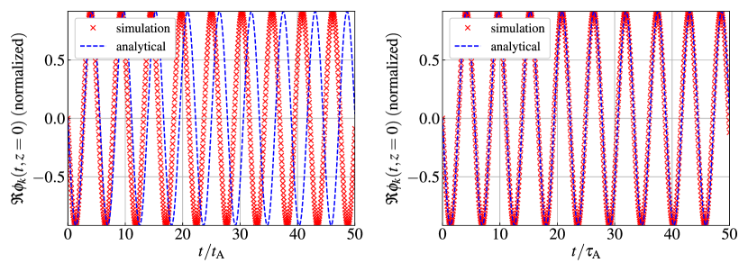
Figure 1: Time evolution of the real part of $\phi_{{\boldsymbol{\mathrm{k}}}_{\perp}}$ for the one-dimensional linear decoupled ITEF. The number of grids in $z$ direction is set to (left) $n_{z}=8$ and (right) $n_{z}=32$.

5.2 Linear Alfvén wave

We next demonstrate that the code correctly captures Alvén wave behavior in the appropriate limit, i.e., $m_{\mathrm{e}}/m_{\mathrm{i}}\to 0$. When the velocity integral terms in (24a)–(24c) are finite, the linearized GKI/ITEF behaves as a damped oscillator due to the ion Landau damping. The dispersion relation for the GKI/ITEF is given by setting $m_{\mathrm{e}}/m_{\mathrm{i}}=0$ for the FGK dispersion relation shown in Ref. [8]. We compare the time evolution solved by the hybrid code with AstroGK with $m_{\mathrm{e}}/m_{\mathrm{i}}=10^{-10}$ where the Alfvén wave is excited by the antenna. The plasma parameters are set to $Z=1$, $\beta_{i}=1$, $\tau=1$, and $k_{\perp}\rho_{\mathrm{i}}=1.0$. For these parameters, GKI/ITEF has frequency and damping rate for the Alfvén wave as $\omega/k_{||}v_{\mathrm{A}}=1.137-0.020i$. The antenna frequency is chosen to be slightly off-resonant, $\omega_{a}/k_{||}v_{\mathrm{A}}=0.9$. The number of grids is set to $(n_{z},\,n_{\lambda},\,n_{E})=(32,\,8,\,32)$. All the fields are initially set to zero. Figure 2 shows the time evolution of $A_{||}$. One finds that the results obtained by both codes agree. The time evolution of GKI/ITEF is fitted by the damped–oscillator solution, then the frequency and damping rate are determined as $\omega/k_{||}v_{\mathrm{A}}=1.142-0.022i$ which is close to the analytical value.

By calculating the time evolution for various $k_{\perp}\rho_{\mathrm{i}}$, we may construct a dispersion diagram. Figure 3 shows the numerical and analytic solutions of the frequency and damping rate of the KAW for several parameter cases, $\beta=1,\,100$ and $\tau=1,\,100$. The grids used are the same as for the above case. The results show good agreement between the numerical and analytical solutions. Whereas the frequencies for FGK and GKI/ITEF are in agreement for all parameters and all $k_{\perp}\rho_{\mathrm{i}}$, there are appreciable differences in the damping rates between FGK and GKI/ITEF for $k_{\perp}\rho_{\mathrm{i}}\gtrsim 1$, except for the $\beta_{\mathrm{i}}=100$ and $\tau=100$ case. This discrepancy is due to the missing electron Landau damping.

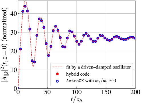
Figure 2: Time evolution of $A_{||}$ solved by the hybrid code (red closed circle) and AstroGK with $m_{\mathrm{e}}/m_{\mathrm{i}}=10^{-10}$ (blue open circle). The red broken line is a fit of the hybrid code result by an analytical solution of the driven–damped oscillator equation.

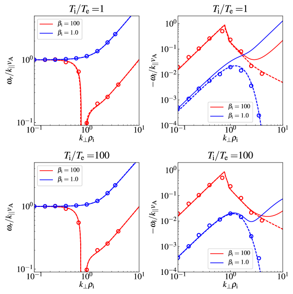
Figure 3: Frequency (left) and damping rate (right) of the KAW for $\beta=1,\,100$ and $\tau=1,\,100$. The solid and broken lines indicate the analytic solutions for FGK and GKI/ITEF, respectively, while the open circles show the result from the simulation.

5.3 Two dimensional Orszag-Tang problem

In this section, we show results of a nonlinear electromagnetic test known as the Orszag-Tang vortex problem [60], which has been regularly used to study decaying MHD turbulence. We compare the results obtained by FGK and GKI/ITEF simulations under the same simulation settings. While there are several variants of initial conditions for the Orszag-Tang problem [61, 62], we use an asymmetric initial condition similar to the one proposed in Ref [62],

$$\phi(x,y) = -\frac{B_{0}}{c}\delta u_{0}\left(\frac{L_{\perp}}{2\pi}\right)\left[\cos\left(\frac{2\pi x}{L_{\perp}}+1.4\right)+\cos\left(\frac{2\pi y}{L_{\perp}}+0.5\right)\right]$$

$$A_{||}(x,y) = \frac{\delta B_{\perp 0}}{2}\left(\frac{L_{\perp}}{2\pi}\right)\left[\frac{1}{2}\cos\left(\frac{4\pi x}{L_{\perp}}+2.3\right)+\cos\left(\frac{2\pi y}{L_{\perp}}+4.1\right)\right],$$ (62)

where $\delta u_{0}$ and $\delta B_{\perp 0}$ represent the initial $E\times B$ drift speed and the initial amplitude of $\delta{\boldsymbol{\mathrm{B}}}_{\perp}=\nabla_{\perp}A_{||}\times\hat{{\boldsymbol{\mathrm{z}}}}$, respectively. Here we have used unnormalized units. In the following test, we choose the initial amplitude so that $\delta u_{0}=\delta B_{\perp 0}/\sqrt{4\pi m_{\mathrm{i}}n_{\mathrm{i}}}$. Below we conduct the simulation in two characteristic spatial regions, the MHD inertial range and the ion kinetic range.

For the MHD inertial range simulation, the domain is set to $L_{\perp}=50\pi\rho_{\mathrm{i}}$ with the number of grid points $(n_{x},n_{y},n_{\lambda},n_{E})=(128,128,8,16)$. This gives a wave number range of $0.02\leq k_{\perp}\rho_{\mathrm{i}}\leq 0.84$. The plasma parameters are set to $\beta_{\mathrm{i}}=1$, $\tau=1$, and $Z=1$. A weak ion collisionality of $\nu_{\mathrm{i}}=0.01\tau_{0}^{-1}$ with $\tau_{0}=L_{\perp}/\delta u_{0}$ is imposed while the electrons are set to collisionless in the FGK simulation. Figure 4 shows the snapshots of $|\delta{\boldsymbol{\mathrm{B}}}_{\perp}|$ at the current sheet formation phase and the turbulence phase. At the current sheet formation phase, the profiles are almost identical between FGK and GK/ITEF. At the turbulent phase, while minor differences are seen in the small scale structures, the large scale structures such as the shape of the filaments are consistent. Figure 5 shows the time evolution of the relative change in the total energy and its components. There is good agreement between the GKI/ITEF and FGK simulations. Since the collisionality employed here is tiny, the total energy $W$ and the 2D invariant $I_{\mathrm{e}}$ are almost conserved. We also conducted a simulation with zero collisionality, and found that the relative errors of $W$ and $I_{\mathrm{e}}$ are within the order of $10^{-5}$ and $10^{-7}$, respectively, until the current sheet formation phase, $t/\tau_{0}\simeq 0.5$ (after this time, collision is necessary to dissipate the small scale energy properly). Figure 6 (left) shows the spectrum of the magnetic energy at the turbulent phase. Both spectra from the GKI/ITEF and FGK simulations agree very well over the entire wave number domain.

Next we show the result of the Orszag-Tang problem for the ion kinetic range. We set the simulation domain to $L_{\perp}=5\pi\rho_{\mathrm{i}}$ with the same number of grids used for the MHD inertial range simulation. The corresponding wave number range is $0.2\leq k_{\perp}\rho_{\mathrm{i}}\leq 8.4$ which spans the transition from the inertial to the kinetic range. Figure 6 (right) shows the magnetic energy spectrum at the turbulent phase. The slope of the spectrum from the GKI/ITEF simulation is shallower than that from the FGK simulation. This observation is consistent with the recent report on the comparison of FGK and a hybrid model composed of full kinetic ion and isothermal electron fluid model [32], although the plasma parameter setting is different. The discrepancy may be attributed to the perpendicular electron damping, which was found to be effective in the ion kinetic region [63].

The improvement of the CFL condition estimated in Section 4 is confirmed by comparison of AstroGK and the hybrid code. Figure 7 shows the time evolution of the maximum advection speed for AstroGK and for the hybrid code in the inertial range and ion kinetic range simulations. In both ranges, the maximum advection speed for GKI/ITEF is due to the ions, and the ITEF does not affect the CFL condition. On the other hand, the maximum advection speed for FGK (presumably dominated by the electron part) is approximately $\sqrt{m_{\mathrm{i}}/m_{\mathrm{e}}}$ times greater than GKI/ITEF, which is consistent with the estimate in Section 4. Using the series data of the maximum convection speed, we calculate the maximum timestep size as a function of time by interpolation. Then, we estimate the minimum number of timestep necessary to reach $t/\tau_{0}=1$, which is 359681 for AstroGK and 8271 for the hybrid code. On the other hand, the averaged computation time per a timestep is 0.756 CPU minutes for AstroGK and 0.430 CPU minutes for the hybrid code at ARCUS (Phase B) in the University of Oxford. Multiplying the computational time per a timestep by the minimum step number, we estimate 4531.98 CPU hours for AstroGK and 59.23 CPU hours for the hybrid code. The improvement of CPU hours is 76.46, which is close to the ideal improvement $2\sqrt{m_{\mathrm{i}}/m_{\mathrm{e}}}\sim 85.7$. The slight fall-off from the ideal improvement is the parallel performance downtick due to the small grid number. We confirmed that the improvement becomes exactly $2\sqrt{m_{\mathrm{i}}/m_{\mathrm{e}}}$ when we increase the velocity grid number as $(n_{\lambda},n_{E})=(8,16)\to(16,32)$.

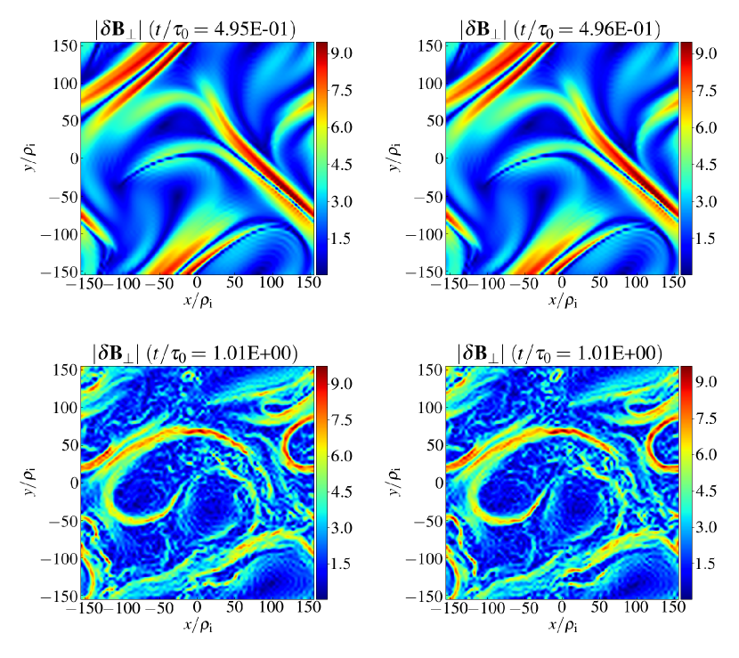
Figure 4: Spatial profiles of $|\delta{\boldsymbol{\mathrm{B}}}_{\perp}|$ for FGK (left) and GKI/ITEF (right) simulations at the current sheet formation phase (top) and the turbulence phase (bottom).

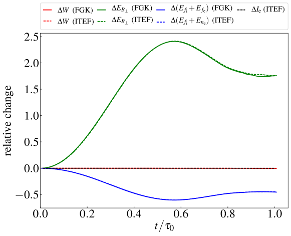
Figure 5: Relative change of total energy and its components from the initial values for the FGK (solid lines) and GKI/ITEF (broken lines) simulations, and the two–dimensional invariant $I_{\mathrm{e}}$ for GKI/ITEF (black broken line).

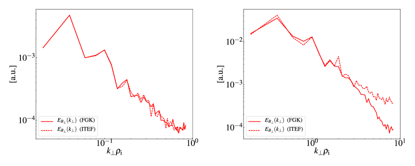
Figure 6: Magnetic energy spectrum for FGK (solid lines) and GKI/ITEF (broken lines) in MHD inertial range (left) and ion kinetic range (right).

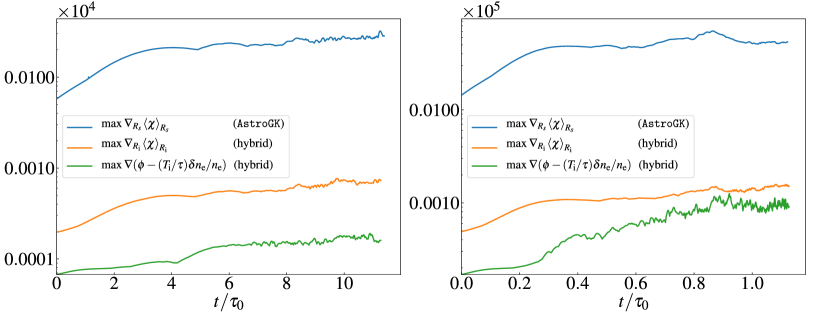
Figure 7: Maximum advection speed for AstroGK and the hybrid code in MHD inertial range (left) and ion kinetic range (right) simulations.

6 Conclusions

A new hybrid simulation code for the GKI/ITEF model [9] has been developed by extending AstroGK, an Eulerian $\delta f$ gyrokinetics code specialized to a slab geometry [41]. We have implemented an algorithm for implicitly solving the coupled system of ITEF and Maxwell’s equations together with the ion gyrokinetic equation. The linear terms are treated by the second-order compact finite difference method while the nonlinear terms are treated by the third-order Adams–Bashforth method. Although the matrix to be inverted for solving the GKI/ITEF-Maxwell’s system of equations is more complicated than that for AstroGK, the computational cost for the inversion is unchanged. Therefore, the hybrid code retains the excellent parallel performance of AstroGK. Since the fast electron timescale is eliminated in the hybrid model, the CFL condition for the explicitly handled nonlinear terms is dramatically less restrictive than for AstroGK. We have estimated and confirmed that the hybrid code runs $2\sqrt{m_{\mathrm{i}}/m_{\mathrm{e}}}\sim 100$ times faster than AstroGK with a single ion species and gyrokinetic electrons.

We also have presented linear and nonlinear tests for code verification. The linear test reproduces the theoretical predictions showing that the implicit algorithm for ITEF is correctly implemented. For the nonlinear test, we conducted the 2D Orszag–Tang vortex problem for spatial scales both larger and smaller than the ion Larmor radius. In the former range, the hybrid code gives a result identical to AstroGK (and also reduced MHD) as theoretically predicted. On the other hand, the power spectrum of GKI/ITEF is shallower than that of FGK at scales smaller than the ion Larmor radius. This is consistent with a recent numerical study comparing FGK and a full kinetic ion and isothermal electron fluid hybrid model [32].

One possible application of the hybrid code is a study on the parametric dependence of ion and electron turbulent heating, which is one of the most important problems in both inner and extra solar systems. At the ion Larmor scale, the energy cascaded from the large scales splits into ion entropy fluctuations and KAWs. It is theoretically predicted that ion entropy fluctuations and KAWs are independently cascaded to smaller scale [9]. The former leads to ion heating while the latter leads to the electron heating. Therefore, the partition of heating by the dissipation of Alfvénic turbulence is determined at the ion Larmor scale, and we do not need to resolve the electron kinetic scale. Since electron kinetics effects are eliminated from the model, we measure only the ion heating occurring around the ion Larmor scale; electron heating may be estimated by assuming that all of the injected energy not dissipated at these scales will ultimately end up heating the electrons. Since the investigation of heating requires high resolution in velocity space, it is computationally cumbersome to scan plasma parameters, e.g., $\beta_{\mathrm{i}}$ and $\tau$. However, with the improved computational efficiency of the hybrid code, such a parameter scan should be feasible.

Another interesting application of the hybrid code is to observe the phase space cascade in 3D electromagnetic turbulence [64, 9, 65]. Whereas the phase space cascade was observed for electrostatic turbulence by AstroGK in a restricted 4D phase space with fine space and velocity grids [44, 45, 47, 46], e.g., $(n_{x},n_{y},n_{\lambda},n_{E})=(256,256,192,96)$ [46], it is unrealistic to conduct similar high resolution simulations for a 5D electromagnetic case with a FGK code. Again, we expect that such simulations are feasible with the present hybrid code at reasonable computational cost.

References

- [1] P. H. Rutherford, E. Frieman, Drift instabilities in general magnetic field configurations, The Physics of Fluids 11 (3) (1968) 569–585. doi:10.1063/1.1691954.
- [2] J. Taylor, R. Hastie, Stability of general plasma equilibria-i formal theory, The Physics of Fluids 10 (5) (1968) 479. doi:10.1088/0032-1028/10/5/301.
- [3] P. J. Catto, Linearized gyro-kinetics, Plasma Physics 20 (7) (1978) 719. doi:10.1088/0032-1028/20/7/011.
- [4] E. Frieman, L. Chen, Nonlinear gyrokinetic equations for low-frequency electromagnetic waves in general plasma equilibria, The Physics of Fluids 25 (3) (1982) 502–508. doi:10.1063/1.863762.
- [5] A. Brizard, T. Hahm, Foundations of nonlinear gyrokinetic theory, Reviews of modern physics 79 (2) (2007) 421. doi:10.1103/RevModPhys.79.421.
- [6] A. M. Dimits, G. Bateman, M. Beer, B. Cohen, W. Dorland, G. Hammett, C. Kim, J. Kinsey, M. Kotschenreuther, A. Kritz, et al., Comparisons and physics basis of tokamak transport models and turbulence simulations, Physics of Plasmas 7 (3) (2000) 969–983. doi:10.1063/1.873896.
- [7] X. Garbet, Y. Idomura, L. Villard, T. Watanabe, Gyrokinetic simulations of turbulent transport, Nuclear Fusion 50 (4) (2010) 043002. doi:10.1088/0029-5515/50/4/043002.
- [8] G. G. Howes, S. C. Cowley, W. Dorland, G. W. Hammett, E. Quataert, A. A. Schekochihin, Astrophysical gyrokinetics: basic equations and linear theory, The Astrophysical Journal 651 (1) (2006) 590. doi:10.1086/506172.
- [9] A. Schekochihin, S. Cowley, W. Dorland, G. Hammett, G. Howes, E. Quataert, T. Tatsuno, Astrophysical gyrokinetics: kinetic and fluid turbulent cascades in magnetized weakly collisional plasmas, The Astrophysical Journal Supplement Series 182 (1) (2009) 310. doi:10.1088/0067-0049/182/1/310.
- [10] G. Howes, W. Dorland, S. Cowley, G. Hammett, E. Quataert, A. Schekochihin, T. Tatsuno, Kinetic simulations of magnetized turbulence in astrophysical plasmas, Physical Review Letters 100 (6) (2008) 065004. doi:10.1103/PhysRevLett.100.065004.
- [11] G. G. Howes, J. M. TenBarge, W. Dorland, E. Quataert, A. A. Schekochihin, R. Numata, T. Tatsuno, Gyrokinetic simulations of solar wind turbulence from ion to electron scales, Physical review letters 107 (3) (2011) 035004. doi:10.1103/PhysRevLett.107.035004.
- [12] J. TenBarge, J. Podesta, K. Klein, G. Howes, Interpreting magnetic variance anisotropy measurements in the solar wind, The Astrophysical Journal 753 (2) (2012) 107. doi:10.1088/0004-637X/753/2/107.
- [13] D. Told, F. Jenko, J. TenBarge, G. Howes, G. Hammett, Multiscale nature of the dissipation range in gyrokinetic simulations of alfvénic turbulence, Physical review letters 115 (2) (2015) 025003. doi:10.1103/PhysRevLett.115.025003.
- [14] A. B. Navarro, B. Teaca, D. Told, D. Groselj, P. Crandall, F. Jenko, Structure of plasma heating in gyrokinetic alfvénic turbulence, Physical Review Letters 117 (24) (2016) 245101. doi:10.1103/PhysRevLett.117.245101.
- [15] G. G. Howes, A prospectus on kinetic heliophysics, Physics of Plasmas 24 (5) (2017) 055907. doi:10.1063/1.4983993.
- [16] S. Bourouaine, G. G. Howes, The development of magnetic field line wander in gyrokinetic plasma turbulence: dependence on amplitude of turbulence, Journal of Plasma Physics 83 (3). doi:10.1017/S0022377817000319.
- [17] K. G. Klein, G. G. Howes, J. M. TenBarge, Diagnosing collisionless energy transfer using field-particle correlations: gyrokinetic turbulence, arXiv preprint arXiv:1705.06385.
- [18] P. B. Snyder, Gyrofluid theory and simulation of electromagnetic turbulence and transport in tokamak plasmas, Ph.D. thesis, Princeton University (1999).
- [19] P. Snyder, G. Hammett, A landau fluid model for electromagnetic plasma microturbulence, Physics of Plasmas 8 (7) (2001) 3199–3216. doi:10.1063/1.1374238.
- [20] A. Sgro, C. Nielson, Hybrid model studies of ion dynamics and magnetic field diffusion during pinch implosions, The Physics of Fluids 19 (1) (1976) 126–133. doi:10.1006/jcph.1994.1084.
- [21] J. Byers, B. Cohen, W. Condit, J. Hanson, Hybrid simulations of quasineutral phenomena in magnetized plasma, Journal of Computational Physics 27 (3) (1978) 363–396. doi:10.1016/0021-9991(78)90016-5.
- [22] D. Hewett, C. Nielson, A multidimensional quasineutral plasma simulation model, Journal of Computational Physics 29 (2) (1978) 219–236. doi:10.1016/0021-9991(78)90153-5.
- [23] D. Hewett, A global method of solving the electron-field equations in a zero-inertia-electron-hybrid plasma simulation code, Journal of Computational Physics 38 (3) (1980) 378–395. doi:10.1016/0021-9991(80)90155-2.
- [24] D. S. Harned, Quasineutral hybrid simulation of macroscopic plasma phenomena, Journal of Computational Physics 47 (3) (1982) 452–462. doi:10.1016/0021-9991(82)90094-8.
- [25] A. P. Matthews, Current advance method and cyclic leapfrog for 2d multispecies hybrid plasma simulations, Journal of Computational Physics 112 (1) (1994) 102–116. doi:10.1006/jcph.1994.1084.
- [26] P. C. Liewer, M. Velli, B. E. Goldstein, Alfvén wave propagation and ion cyclotron interactions in the expanding solar wind: One-dimensional hybrid simulations, Physical Review Letters 106 (A12) (2001) 29261–29281. doi:10.1029/2001JA000086.
- [27] P. Hellinger, P. Trávníček, A. Mangeney, R. Grappin, Hybrid simulations of the expanding solar wind: Temperatures and drift velocities, Geophysical research letters 30 (5). doi:10.1029/2002GL016409.
- [28] P. Hellinger, P. Trávníček, Magnetosheath compression: Role of characteristic compression time, alpha particle abundance, and alpha/proton relative velocity, Journal of Geophysical Research: Space Physics 110 (A4). doi:10.1029/2004JA010687.
- [29] M. W. Kunz, J. M. Stone, X.-N. Bai, Pegasus: A new hybrid-kinetic particle-in-cell code for astrophysical plasma dynamics, Journal of Computational Physics 259 (2014) 154–174. doi:10.1016/j.jcp.2013.11.035.
- [30] M. W. Kunz, J. M. Stone, E. Quataert, Magnetorotational turbulence and dynamo in a collisionless plasma, Physical Review Letters 117 (23) (2016) 235101. doi:10.1103/PhysRevLett.117.235101.
- [31] S. Cerri, L. Franci, F. Califano, S. Landi, P. Hellinger, Plasma turbulence at ion scales: a comparison between particle in cell and eulerian hybrid-kinetic approaches, Journal of Plasma Physics 83 (2). doi:10.1017/S0022377817000265.
- [32] D. Groselj, S. S. Cerri, A. B. Navarro, C. Willmott, D. Told, N. F. Loureiro, F. Califano, F. Jenko, Fully-kinetic versus reduced-kinetic modelling of collisionless plasma turbulence, arXiv preprint arXiv:1706.02652.
- [33] F. Valentini, P. Trávníček, F. Califano, P. Hellinger, A. Mangeney, A hybrid-vlasov model based on the current advance method for the simulation of collisionless magnetized plasma, Journal of Computational Physics 225 (1) (2007) 753–770. doi:10.1016/j.jcp.2007.01.001.
- [34] Z. Lin, L. Chen, A fluid–kinetic hybrid electron model for electromagnetic simulations, Physics of Plasmas 8 (5) (2001) 1447–1450. doi:10.1063/1.1356438.
- [35] Y. Chen, S. Parker, A gyrokinetic ion zero electron inertia fluid electron model for turbulence simulations, Physics of Plasmas 8 (2) (2001) 441–446. doi:10.1063/1.1335584.
- [36] P. Snyder, G. Hammett, Electromagnetic effects on plasma microturbulence and transport, Physics of Plasmas 8 (3) (2001) 744–749. doi:10.1063/1.1342029.
- [37] S. E. Parker, Y. Chen, C. C. Kim, Electromagnetic gyrokinetic-ion drift-fluid-electron hybrid simulation, Computer physics communications 127 (1) (2000) 59–70. doi:10.1016/S0010-4655(00)00027-8.
- [38] I. Abel, S. Cowley, Multiscale gyrokinetics for rotating tokamak plasmas: Ii. reduced models for electron dynamics, New Journal of Physics 15 (2) (2013) 023041. doi:10.1088/1367-2630/15/2/023041.
- [39] F. Hinton, M. Rosenbluth, R. Waltz, Reduced equations for electromagnetic turbulence in tokamaks, Physics of Plasmas 10 (1) (2003) 168–178. doi:10.1063/1.1524630.
- [40] R. Hager, J. Lang, C.-S. Chang, S. Ku, Y. Chen, S. E. Parker, M. F. Adams, Verification of long wavelength electromagnetic modes with a gyrokinetic-fluid hybrid model in the xgc code, Physics of Plasmas 24 (5) (2017) 054508. doi:10.1063/1.4983320.
- [41] R. Numata, G. G. Howes, T. Tatsuno, M. Barnes, W. Dorland, Astrogk: Astrophysical gyrokinetics code, Journal of Computational Physics 229 (24) (2010) 9347–9372. doi:10.1016/j.jcp.2010.09.006.
- [42] M. Kotschenreuther, G. Rewoldt, W. Tang, Comparison of initial value and eigenvalue codes for kinetic toroidal plasma instabilities, Computer Physics Communications 88 (2) (1995) 128–140. doi:10.1016/0010-4655(95)00035-E.
- [43] W. Dorland, F. Jenko, M. Kotschenreuther, B. Rogers, Electron temperature gradient turbulence, Physical Review Letters 85 (26) (2000) 5579. doi:10.1103/PhysRevLett.85.5579.
- [44] T. Tatsuno, W. Dorland, A. Schekochihin, G. Plunk, M. Barnes, S. Cowley, G. Howes, Nonlinear phase mixing and phase-space cascade of entropy in gyrokinetic plasma turbulence, Physical review letters 103 (1) (2009) 015003. doi:10.1103/PhysRevLett.103.015003.
- [45] T. Tatsuno, M. Barnes, W. Dorland, R. Numata, G. Plunk, S. Cowley, G. Howes, A. Schekochihin, Gyrokinetic simulation of entropy cascade in two-dimensional electrostatic turbulence, Journal of Plasma and Fusion Research SERIES 9 (2010) 509–516.
- [46] T. Tatsuno, G. Plunk, M. Barnes, W. Dorland, G. Howes, R. Numata, Freely decaying turbulence in two-dimensional electrostatic gyrokinetics, Physics of Plasmas 19 (12) (2012) 122305. doi:10.1063/1.4769029.
- [47] G. Plunk, T. Tatsuno, Energy transfer and dual cascade in kinetic magnetized plasma turbulence, Physical review letters 106 (16) (2011) 165003. doi:10.1103/PhysRevLett.106.165003.
- [48] R. Numata, W. Dorland, G. G. Howes, N. F. Loureiro, B. N. Rogers, T. Tatsuno, Gyrokinetic simulations of the tearing instability, Physics of Plasmas 18 (11) (2011) 112106. doi:10.1063/1.3659035.
- [49] S. Kobayashi, B. N. Rogers, R. Numata, Gyrokinetic simulations of collisionless reconnection in turbulent non-uniform plasmas, Physics of Plasmas 21 (4) (2014) 040704. doi:10.1063/1.4873703.
- [50] R. Numata, N. Loureiro, Ion and electron heating during magnetic reconnection in weakly collisional plasmas, Journal of Plasma Physics 81 (02) (2015) 305810201. doi:10.1017/S002237781400107X.
- [51] A. Zocco, N. Loureiro, D. Dickinson, R. Numata, C. Roach, Kinetic microtearing modes and reconnecting modes in strongly magnetised slab plasmas, Plasma Physics and Controlled Fusion 57 (6) (2015) 065008. doi:10.1088/0741-3335/57/6/065008.
- [52] I. Abel, M. Barnes, S. Cowley, W. Dorland, A. Schekochihin, Linearized model fokker–planck collision operators for gyrokinetic simulations. i. theory, Physics of Plasmas 15 (12) (2008) 122509. doi:10.1063/1.3046067.
- [53] M. Barnes, I. Abel, W. Dorland, D. Ernst, G. Hammett, P. Ricci, B. Rogers, A. Schekochihin, T. Tatsuno, Linearized model fokker–planck collision operators for gyrokinetic simulations. ii. numerical implementation and tests, Physics of Plasmas 16 (7) (2009) 072107. doi:10.1063/1.3155085.
- [54] Y. Kawazura, M. Barnes, A. A. Schekochihin, in preparation.
- [55] R. Courant, K. Friedrichs, H. Lewy, On the partial difference equations of mathematical physics, IBM journal 11 (2) (1967) 215–234.
- [56] R. M. Beam, R. F. Warming, An implicit finite-difference algorithm for hyperbolic systems in conservation-law form, Journal of computational physics 22 (1) (1976) 87–110. doi:10.1016/0021-9991(76)90110-8.
- [57] S. A. Orszag, On the elimination of aliasing in finite-difference schemes by filtering high-wavenumber components, Journal of the Atmospheric sciences 28 (6) (1971) 1074–1074.
- [58] J. TenBarge, G. G. Howes, W. Dorland, G. W. Hammett, An oscillating langevin antenna for driving plasma turbulence simulations, Computer Physics Communications 185 (2) (2014) 578–589. doi:10.1016/j.cpc.2013.10.022.
- [59] P. Goldreich, S. Sridhar, Toward a theory of interstellar turbulence. 2: Strong alfvenic turbulence, The Astrophysical Journal 438 (1995) 763–775. doi:10.1086/175121.
- [60] S. A. Orszag, C.-M. Tang, Small-scale structure of two-dimensional magnetohydrodynamic turbulence, Journal of Fluid Mechanics 90 (01) (1979) 129–143. doi:10.1017/S002211207900210X.
- [61] D. Biskamp, H. Welter, Dynamics of decaying two-dimensional magnetohydrodynamic turbulence, Physics of Fluids B: Plasma Physics 1 (10) (1989) 1964–1979. doi:10.1063/1.859060.
- [62] N. Loureiro, W. Dorland, L. Fazendeiro, A. Kanekar, A. Mallet, M. Vilelas, A. Zocco, Viriato: A fourier–hermite spectral code for strongly magnetized fluid–kinetic plasma dynamics, Computer Physics Communications 206 (2016) 45–63. doi:10.1016/j.cpc.2016.05.004.
- [63] T. C. Li, G. G. Howes, K. G. Klein, J. M. TenBarge, Energy dissipation and landau damping in two-and three-dimensional plasma turbulence, The Astrophysical Journal Letters 832 (2) (2016) L24. doi:10.3847/2041-8205/832/2/L24.
- [64] A. Schekochihin, S. Cowley, W. Dorland, G. Hammett, G. Howes, G. Plunk, E. Quataert, T. Tatsuno, Gyrokinetic turbulence: a nonlinear route to dissipation through phase space, Plasma Physics and Controlled Fusion 50 (12) (2008) 124024. doi:10.1088/0741-3335/50/12/124024.
- [65] G. Plunk, S. Cowley, A. Schekochihin, T. Tatsuno, Two-dimensional gyrokinetic turbulence, Journal of Fluid Mechanics 664 (2010) 407–435. doi:10.1017/S002211201000371X.