Eddy energy sources and mesoscale eddies in the Sea of Okhotsk.

Abstract

Based on an eddy-permitting ocean circulation model, the eddy kinetic energy (EKE) sources are studied in the Sea of Okhotsk. An analysis of the spatial distribution of the EKE showed that intense mesoscale variability occurs along the western boundary of the Sea of Okhotsk, where the East-Sakhalin Current extends. It was found a pronounced seasonally varying EKE with its maximal magnitudes in winter, and its minimal magnitudes in summer.

An analysis of the EKE sources and the energy conversions showed that time-varying (turbulent) wind stress is a main contribution to mesoscale variability along the western boundary of the Sea of Okhotsk. The contribution of baroclinic instability to the generation of mesoscale variability predominates over that of barotropic instability along the western boundary of the Sea of Okhotsk.

To demonstrate the mechanism of baroclinic instability, the circulation was considered along the western boundary of the Sea of Okhotsk from January to April 2005. An analysis of hydrological conditions showed outcropping isopycnals and being strong vertical shear of the along-shore velocity from January to May 2005. In April, mesoscale eddies are observed along the western boundary of the Sea of Okhotsk. It was established that seasonal variability of turbulent wind stress and the baroclinic instability of the East-Sakhalin Current are major reasons of mesoscale variability along the western boundary of the Sea of Okhotsk.

1 Introduction

The Sea of Okhotsk is one of the marginal seas in the north-western Pacific Ocean. This sea is situated at high latitudes and being the southernmost sea, covered by sea ice during the year. The sea ice covering period begins from the end of November and can last up to the end of May. It complicates significantly to carry out observations in the Sea of Okhotsk.

The Okhotsk Sea circulation is the subject of high scientific interest Ohshima2002 ; Mizuta2003 , because this basin is the source of intermediate water in the western North Pacific Talley1991 ; Gladyshev2003 ; Fukamachi2004 . Dense shelf waters, generated over the north-west shelf of the Sea of Okhotsk in winter, are transported by the East-Sakhalin Current (ESC) in the Kuril Basin, where they are mixed by mesoscale eddies and tides. Scherbina et al.  Shcherbina2004a , based on datasets obtained from the moorings deployed at the north-western this sea, discovered sharp changes in the density increase in late February. Authors supposed that these sharp density changes were induced by baroclinic instability of the density front.

The basic element of the basin-scale circulation in the Sea of Okhotsk is the ESC, which extends from the north-western to the southern part of this sea. In the south-western Sea of Okhotsk, the Kuril Basin is situated with the depth exceeding 3000 m. The anticyclonic circulation occurs over the Kuril Basin. The Sea of Okhotsk interacts with the Japan/East Sea by means of the Soy and Tatar Straits and with the North Pacific Ocean by means of the Kuril Straits.

Numerous studies investigated reasons and mechanisms of the basin-scale circulation in the Sea of Okhotsk. According to Ohshima2002 ; Smizu2006 , it is supposed that the wind stress is the major driver of the basin-scale circulation in the Sea of Okhotsk. The dominating positive wind stress curl over the Sea of Okhotsk drives cyclonic circulation in the central part of this sea. In addition, the along-shore wind stress component is the major driver of the along–shore branch of the ESC. Because of strong seasonal variability of the wind stress, the intensity of the Okhotsk Sea circulation also exhibits strong seasonal variability. In addition, heat and freshwater fluxes over the Sea of Okhotsk exhibit seasonal variability and their impact on the basin-scale circulation is corrected by ice covering.

Mesoscale eddies in the Sea of Okhotsk are the subject of intensive investigations. Ohshima et al. Ohshima2002 , based on satellite-tracked drifter observations, revealed that anticyclonic eddies with the diameter varying from 100 to 200 km dominate over the Kuril Basin and eddy kinetic energy exceeds mean kinetic energy from 3 to 20 times. Ohshima et al. Ohshima2005 established that the major mechanism of eddy generation over the Kuril Basin is the baroclinic instability of the tidal front induced by intense tidal mixing near the Kuril Straits. Ohshima et al. Ohshima1990 investigated mesoscale variability over the south-western Kuril Basin near the Soya Strait. It was established that the mechanism of eddy generation is the barotropic instability of the Soya Current. The impact of the Soya Current transport on mesoscale variability was studied by Uchimoto2007 . Thermal infrared images with very high spatial resolution showed features of sub-mesoscale variability (the eddy diameter ranging from 2 to 30 km) near the Kuril Islands Nakamura2012 .

In the above mentioned studies, mesoscale variability in the Sea of Okhotsk was studied mainly during the ice-free period. Thus, the whole picture of mesoscale variability in the Sea of Okhotsk does not fully understand. Because of challenge of the carrying out natural observations during the sea ice covering period, at studying the Okhotsk Sea circulation, the numerical models are applied, which are accounting for mesoscale variability. It should be noted that according to the work Chelton1998 , at high latitudes the first baroclinic Rossby radius of deformation $(\lambda_{1})$ is significantly less than that at middle and low latitudes. Low values of $\lambda_{1}$ constrain spatial resolution of the model grid, which needs to explicitly resolve mesoscale variability in the Sea of Okhotsk. In addition, $\lambda_{1}$ magnitudes can exhibit significant spatial and time variability due to strong irregularity of the bottom topography and seasonal variability of density stratification in the Sea of Okhotsk. Numerical simulations of the circulation in the Sea of Okhotsk with high spatial resolution were presented in a number of works. Based on numerical simulations with the grid resolution of 3 km, Matsuda et al. Matsuda2015 ; Matsuda2009 analyzed ventilation processes in the intermediate layer of the Sea of Okhotsk. However, reasons and mechanisms of mesoscale variability in the Sea of Okhotsk have not fully revealed.

At investigating mesoscale variability both the World Ocean and marginal seas, the one of the approaches is based on the analysis of the eddy kinetic energy (EKE) budget. von Storch et al. Storch2012 presented the methodology and carried out the comprehensive analysis of the sources and sinks of the EKE in the World Ocean based on numerical simulations. They assessed contributions of baroclinic and barotropic instabilities of the large-scale currents to the generation of mesoscale variability.

Based on this methodology, the EKE budget and mechanisms of mesoscale variability have examined in the Red Sea, the South China Sea and the Labrador Sea. Based on the outputs of the high-resolution MITgcm, Zhan et al. Zhan2016 established that the leading mechanism of the eddy generation in the Red Sea is baroclinic instability, whereas turbulent wind stress and barotropic instability influence weakly on mesoscale variability in this sea. Based on the outputs of the high-resolution LICOM, Yang et al. Yang2013 established that both hydrodynamic instability and wind power input influence significantly on mesoscale variability in the South China Sea. Eden et al. Eden2002 , based on the outputs of the MOM, established that the barotropic instability of the West Greenland Current is the major source of EKE in the Labrador Sea. Thus, depending on the considered basin, contributions of wind power input, baroclinic instability and barotropic instability to EKE can be different Storch2012 .

In this study, based on the numerical simulations, mesoscale variability is analyzed in the Sea of Okhotsk. Wind power input, baroclinic and barotropic instabilities of the ESC are considered as the main sources of the EKE. The paper is organized as follows. Sect. 2 describes the model configuration and validation of its outputs. Spatial and temporal analysis of EKE in the Sea of Okhotsk is presented in Sect. 3. An analysis of eddy energy conversion from the mean circulation is presented in Sect. 4. Sect. 5 presents estimations of the main sources of EKE in the Sea of Okhotsk. Typical picture of mesoscale variability on the eastern shelf of Sakhalin Island induced by baroclinic instability of the ESC is presented in Sect. 6. Discussion and summary of the main results are presented in Sect. 7.

2 Model setup and validation

To simulate the circulation in the Sea of Okhotsk, an INMOM model is applied with the horizontal resolution of about 3.5 km and 35 sigma-levels compressed toward the sea surface to resolve density stratification. The INMOM is the sigma-coordinate model based on primitive equations of ocean dynamics with hydrostatic and Boussinesq approximations Gusev2014 ; Stepanov2014 ; Diansky2016 . The model domain covers the Sea of Okhotsk, the Japan/East Sea and the north-western Pacific Ocean to take into consideration the water exchange between of them. To obtain quasi-uniform spatial resolution, the spherical coordinate system with the pole, situated at the point with the coordinates of (25.5^∘E, 22.4^∘N), is used. Thus, an equator of a new coordinate system crosses the Sea of Okhotsk and the Japan/East Sea.

To account for mesoscale variability in the Sea of Okhotsk, it is necessarily that the spatial scale of the model grid and $\lambda_{1}$ are the same order. Preliminarily, $\lambda_{1}$ was assessed with the relationship Chelton1998 ,

$$\lambda_{1}=\frac{c_{1}}{|f|},$$ (1)

where $f=2\Omega\sin\vartheta$ is the Coriolis parameter, $\Omega$ is the Earth rotation rate, $\vartheta$ is the latitude and $c_{1}$ is the first eigenvalue, which satisfies the boundary value problem

$$\begin{array}[]{l}\frac{d^{2}}{dz^{2}}\phi_{1}+\frac{N^{2}(z)}{c_{1}^{2}}\phi_{1}=0,\\ \phi_{1}(0)=\phi_{1}(-H)=0.\end{array}$$ (2)

Here, the vertical coordinate $z$ directs from the center of the Earth, $N(z)$ is the buoyancy frequency profile, $H$ is the depth and $\phi_{1}(z)$ is the first eigenfunction of the boundary value problem (2). According to Chelton1998 , c₁ can be assessed as

$$c_{1}\approx\frac{1}{\pi}\int_{-H}^{0}N(\xi)d\xi.$$ (3)

Based on climatological monthly mean temperature and salinity fields of datasets Locarnini2013 ; Zweng2013 , $\lambda_{1}$ was assessed. These fields have the horizontal resolution of 0.25^∘ and to be arranged at 102 horizons.

Fig. 1 shows an annual mean distribution of $\lambda_{1}$ in the Sea of Okhotsk. According to the obtained estimations, maximum magnitude of $\lambda_{1}$, amounting to 20 km, occurs in the south-western Sea of Okhotsk over the Kuril Basin. Over the central part of the Sea of Okhotsk, $\lambda_{1}$ magnitude varies from 10 to 12 km and from 3 to 9 km along the western boundary of this sea. Minimal values of $\lambda_{1}$ occur in the north-eastern Sea of Okhotsk and range from 1 to 2 km. Thus, the used horizontal resolution is the eddy-permitting resolution except the north-eastern and northern part of the Sea of Okhotsk, where the spatial scale of the model grid is higher than $\lambda_{1}$.

Bottom topography of the model domain was extracted from the GEBCO dataset Becker2009 and to be smoothed by the 9-point filter. Sensible and latent heat fluxes, short- and long-wave radiation, momentum flux and net salt flux, containing precipitation, evaporation and climatological runoff contributions, are set with the bulk-formulae Stepanov2014 ; Diansky2016 ; Large2009 . Atmospheric parameters were extracted from the ERA-Interim dataset Dee2011 with the spatial resolution of 0.75${}^{\circ}\times$0.75^∘ from 1979 to 2009. It should be noted that wind velocity field at the high of 10 m, air temperature and absolute humidity at the 2 m, as well as sea level pressure have the time-resolution of 6 hours. To correctly account for the interaction between the circulation in the Sea of Okhotsk and atmospheric forcing, the INMOM includes a sea-ice model. This model accounts for processes of generation and melting of sea ice and transforming of stale snow to sea ice Yakovlev2003 . At the same time, wind stress over the Sea of Okhotsk is calculated under the open water condition, that is, the sea ice covering is absent. The approximation of the open water is correct, when the sea ice compactness is less than 0.75. When the sea ice compactness is more than 0.75, then the approximation of the open water accounts for the impact of the moving ice on the sea water.

Initial potential temperature and salinity are extracted from the datasets Locarnini2013 ; Zweng2013 . On the sea surface, potential temperature and salinity are corrected by adding their climatological values to the heat and salinity fluxes with the relaxation parameter amounts to 10/3 m month^-1. This procedure removes the climatological drift of the circulation in the Sea of Okhotsk induced by uncertainties of atmospheric parameters. It should be noted that the presented model configuration does not account for the tidal impact on the circulation in the Sea of Okhotsk.

On the open boundary of the model domain, no-normal and no-slip flow conditions are set. In narrow regions near the open boundaries from the sea surface to bottom, the nudging condition is set for potential temperature and salinity with the relaxation parameter of 3 hours.

The sub-grid processes are parameterized with the viscosity operator of the second order with the coefficient of 100 m² s^-1. The horizontal diffusion of heat and salt, formulated along the geopotential surfaces, are parameterized with the viscosity operator of the second order with the coefficient of 10 m² s^-1 for both variables. The vertical turbulent processes are parameterized according to Pacanowski1981 and vertical viscosity and diffusivity amount to 10^-4 m² s^-1 and 10^-5 m² s^-1, respectively. Convective mixing is parameterized by maximum viscosity and diffusivity, which amount to 2.5$\times$10^-2 m² s^-1 and 5$\times$10^-3 m² s^-1, respectively.

Preliminarily, we simulated circulation during four years with the atmospheric forcing corresponding to 1979. Initial conditions for potential temperature and salinity corresponded to June. Thus, we avoided setting up initial compactness and height of sea ice in our model configuration. Model outputs, obtained in the end of fourth year of numerical simulations, were used as initial conditions for the numerical simulations with the atmospheric forcing varying from 1979 to 2009.

In this study, we analyze the model outputs from 2005 to 2009. Fig. 2 shows a long–term mean (from 2005 to 2009) of a velocity field at the horizon of 10 m, as well as a mean of wind power input $(\overline{\mathbf{\tau}}\cdot\overline{\mathbf{u}_{s}})$, where $\overline{\mathbf{\tau}},\overline{\mathbf{u}_{s}}$ are the wind stress and sea surface currents averaged for the season, respectively.

In winter, maximal velocities, varying from 0.3 to 0.4 m s^-1, occur along the western boundary of the Sea of Okhotsk, where the ESC extends. Along the norther boundary of the Sea of Okhotsk and over the Kuril Basin, it is observed less intense currents with velocities ranging from 0.1 to 0.15 m s^-1. In addition, maximal wind power input, amounting to 4$\times$10^-2 W m^-2, occurs over the western and northern boundaries of the Sea of Okhotsk. Positive values of $(\overline{\mathbf{\tau}}\cdot\overline{\mathbf{u}_{s}})$ indicate that the current direction coincides with the direction of mean wind stress, except a small region is situated near the eastern boundary of the Sea of Okhotsk. From spring to summer, the simulated circulation weakens significantly. Velocities in the ESC weaken from 0.2 m s^-1 to 0.1 m s^-1 and current direction in the western of the Sea of Okhotsk changes opposite to direction of wind stress, which weakens up to –0.2$\times$10^-2 W m^-2. In autumn, the simulated circulation strengthens again in the northern and the western Sea of Okhotsk up to 0.2–0.25 m s^-1. At the same time, mean wind power input increases up to 2.5$\times$10^-2 W m^-2. It should be noted that $(\overline{\mathbf{\tau}}\cdot\overline{\mathbf{u}_{s}})$ shows its positive values in the regions of intense currents along the western and northern boundaries of the Sea of Okhotsk. The simulated surface circulation is similar that obtained from the natural observations Moroshkin1966 ; Luchin1998 and the spatial distribution of mean wind power input does not contradict conclusions about significant influence of wind stress on the basin-scale circulation in the Sea of Okhotsk.

Because the ESC is the most intense current in the structure of the simulated circulation, we will concentrate on the velocity field along the western boundary of the Sea of Okhotsk. The simulated circulation shows that the ESC consists of two branches (cores). The first branch of this current onsets in the north-western Sea of Okhotsk. The second branch of the ESC is the element of the basin-scale cyclonic gyre covering the central part of this sea. An analysis of the simulated velocity field shows that the ESC exhibits strong seasonal variability (not shown). At the horizon of 20 m, monthly mean velocities in the first and second branches of the ESC reach to 0.3 m s^-1 and 0.1 m s^-1, respectively. In spring, velocities in the first branch of the ESC decrease up to 0.21 m s^-1. In the end of summer, the intensity of the ESC is minimal. On the eastern shelf of Sakhalin Island, monthly mean velocities are limited by the value of 0.15 m s^-1. In autumn, the simulated velocities in the ESC increase again up to 0.32 m s^-1.

The estimation of the annual mean ESC transport shows that in winter it reaches the value of 6 Sv. In summer, the ESC transport shows its minimal magnitudes ranging from 1.5 to 2 Sv. The obtained estimation of the ESC transport and its season variability are similar with that obtained from the natural observations Ohshima2002 and numerical simulations of the Sea of Okhotsk circulation Matsuda2015 . Comparing the results of the simulated circulation with those of the previous studies shows that the mean simulated circulation is correct and to be characterized by the occurrence of the north current along the western boundary of the Sea of Okhotsk. This north current consists of two branches and features seasonal variability with maximum intensity in winter and minimum intensity in late summer. The subject of next sections is mesoscale variability and its main sources mainly along the western boundary of the Sea of Okhotsk.

3 Eddy kinetic energy in the Okhotsk Sea

In this section, based on the model outputs, the EKE in the Sea of Okhotsk is analyzed from 2005 to 2009. Eddy or non-stationary component denotes a deflection from its mean value. Because of strong seasonal signal in the simulated circulation, the monthly averaging is applied from 2005 to 2009. It is considered four seasons: winter (January, February, and March), spring (April, May and June), summer (July, August and September) and autumn (October, November and December). The EKE is given by the relation

$$EKE=\frac{1}{2}\rho_{0}\left(\overline{u^{\prime 2}}+\overline{v^{\prime 2}}\right).$$ (4)

where $\rho_{0}$ is the density reference, amounting to 1025 kg m^-1, and $\overline{u^{\prime 2}}$, $\overline{v^{\prime 2}}$ are the monthly mean squares of the eddy component of zonal and meridional velocity, respectively. The primes and overbars denote deflections from the long-term monthly mean and the time averaging, respectively. $\overline{u^{\prime 2}}$, $\overline{v^{\prime 2}}$ are assessed with the relation Storch2012

$$\overline{x^{\prime}\cdot y^{\prime}}=\overline{x\cdot y}-\overline{x}\cdot\overline{y},$$ (5)

where $x,y$ are the current velocity components (or density deflection from its reference value), which are extracted from the model outputs with the time period of 1 day. Besides, kinetic energy of mean currents (MKE) is assessed with the relation

$$MKE=\frac{1}{2}\rho_{0}\left(\overline{u}^{2}+\overline{v}^{2}\right).$$ (6)

Fig. 3 shows the vertical profiles of EKE and MKE are averaged over the whole basin. In winter, the EKE reaches its maximal magnitudes, amounting to 15 J m^-3, near the sea surface. The EKE magnitudes exceed the MKE magnitudes up to 2.5 times. In summer, EKE and MKE decrease to 8 J m^-3 and 1.2 J m^-3, respectively. Vertical profiles of EKE and MKE indicate that intense dynamics occurs in the upper 200 m of the Sea of Okhotsk. Below this layer, EKE and MKE magnitudes reach their low values, amounting to about 1 J m^-3, for both seasons. Further, we will consider EKE variability in the upper 200 m, only.

Fig. 4 shows the spatial distribution of EKE, integrated in the upper 200 m, during different seasons. In winter, EKE reach its maximum value, amounting to 3.5$\times$10³ J m^-2, along the western boundary of the Sea of Okhotsk and in the south-western Kuril Basin. It should be noted that a region with maximal magnitudes of EKE, ranging from 0.9$\times$10³ to 2.2$\times$10³ J m^-2, covers a wide area along the western boundary of the Sea of Okhotsk, which results from different places of mesoscale eddy generation. A region, situated northward 52^∘N, where EKE magnitudes range from 0.45 to 0.9$\times$10³ J m^-2, widens from 144^∘E to 149^∘E due to strong hydrodynamic instability of the ESC. Over the Kuril Basin, along the eastern boundary and on the north-eastern of the Sea of Okhotsk, EKE magnitudes are limited by 0.45$\times$10³ J m^-2. In spring, the intensity of mesoscale variability decreases over the whole basin. Along the western boundary of the Sea of Okhotsk, EKE decreases up to 0.9$\times$10³ J m${}^{-}{2}$. Decreasing EKE up to 0.75$\times$10³ J m^-2 is observed in the south-western Sea of Okhotsk. A small region with the EKE magnitudes, exceeding 1.5$\times$10³ J m^-2, is situated northward 44^∘N. In other regions of this sea, the EKE magnitudes are limited by 0.3$\times$10³ J m^-2. In summer, EKE magnitudes shows minimal values, ranging from 0.15$\times$10³ to 0.3$\times$10³ J m^-2, for the whole basin. Along the western boundary of the Sea of Okhotsk, the EKE magnitudes are limited by 0.6$\times$10³ J m^-2. In autumn, the intensity of mesoscale variability increases again in the Sea of Okhotsk. The spatial distribution of EKE shows its maximal magnitudes, amounting to up 2$\times$10³ J m^-2. Along the western boundary, in the southern basin and along the eastern part of this sea, the EKE magnitudes reach to 0.6$\times$10³ J m^-2.

Thus, the intense mesoscale variability in the Sea of Okhotsk is observed in upper 200 m, where the EKE magnitudes exceed more than 2.5 times those of MKE in winter and about 9 times in summer. The spatial distribution of EKE revels the pronounced seasonally varying EKE with its maximal values in winter and its minimal values in summer. According to the spatial distributions of EKE, its maximal values appear along the western boundary of the Sea of Okhotsk, where the ESC extends, during different seasons. According to the natural observations Mizuta2003 and results of previous numerical simulations Smizu2006 ; Matsuda2015 , the transport of the ESC is characterized by strong seasonal variability. This transport reaches its maximal values in winter and its minimal values in the end of summer. It is supposed that seasonal variability of mesoscale variability can be results from the hydrodynamic instability of the ESC.

4 Energy conversion in the Sea of Okhotsk

According to results of the previous section, the EKE maximal magnitudes were observed along the western boundary of the Sea of Okhotsk, where the ESC extends, during different seasons. It is supposed that hydrodynamics instability (baroclinic and barotropic) of the along-shore branch of the ESC induces intense mesoscale variability associated with high EKE magnitudes. To examine this supposition, two quantities are analyzed in this section. The first quantity (BC) estimates quantitatively the rate of energy conversion from the mean available potential energy (MPE) to eddy available potential energy (EPE) and characterizes the baroclinic instability of the ESC. The second quantity (BT) is linked with the rate of energy conversion from MKE to EKE and characterizes the barotropic instability of the ESC. To estimate the BC, it is used the following relation Thomson1984 ; Eden2002 ; Zhan2016

$$BC=-\frac{g^{2}}{\overline{N}^{2}\rho_{0}}\overline{\mathbf{u^{\prime}}_{h}\rho^{\prime}}\cdot\nabla_{h}\overline{\rho},$$ (7)

where $\nabla_{h}$ is the horizontal operator, $g$ is the gravitational acceleration, $\overline{N}^{2}$ is the basin-averaged square of the buoyancy frequency Storch2012 , $\mathbf{u}_{h}$ is the horizontal velocities and $\rho$ is the density deflection from the reference value $\rho_{0}$. To assess an eddy density flux $(\overline{\mathbf{u^{\prime}}_{h}\rho^{\prime}})$, it was used the relation (5). According to (7), negative BC indicates that EPE is converted to MPE, when $\overline{\mathbf{u^{\prime}}_{h}\rho^{\prime}}$ is directed in the same direction with the horizontal gradient of mean density. On the other hand, when the BC$>$0, then $\overline{\mathbf{u^{\prime}}_{h}\rho^{\prime}}$ is against the direction of mean density gradient, that is, MPE is converted to EPE.

Fig. 5 shows spatial distributions of the BC, integrated in the upper 200 m during different seasons. According to these distributions, maximal magnitudes of the BC occur along the western boundary of the Sea of Okhotsk in winter, when the rate of energy conversion from MPE to EPE exceeds to 6$\times$10^-2 W m^-2. In the other regions of the Sea of Okhotsk, the BC magnitudes are two times less than those along the western boundary of this sea. In spring, the path of energy conversion from EPE to MPE predominates along the eastern and western boundaries of the Sea of Okhotsk. The BC reaches its minimal values in summer, when the rate of energy conversion from MPE to EPE is limited by 10^-3 W m^-2. In autumn, high magnitudes of the BC, amounting to 5$\times$10^-2 W m^-2, occur along the western boundary of the Sea of Okhotsk. However, the autumn distribution of the BC is very heterogeneous and the spots of positive values of the BC alternate with those of negative values of the BC. This heterogeneity of the BC distribution does not allow single out the predominant path of energy conversion with the exception of a small region northern 52^∘N along the western boundary of the Sea of Okhotsk, where the path of energy conversion from MPE to EPE predominates.

It should be noted that positive magnitudes of the BC predominate during different seasons in the south-western Kuril Basin. Despite on low positive magnitudes of the BC over the Kuril Basin, limited by the value of 1-2$\times$10^-2 W m^-2, it indicates that the path of energy conversion from MPE to EPE predominates. In addition, it coincides with the result of the previous work Ohshima2005 , where the predominant influence of baroclinic instability on mesoscale variability has been revealed over the Kuril Basin. However, low values of the BC are probably induced by the underestimate of the tidal mixing, generating the frontal zone in the southern Kuril Basin.

To analyze the contribution of the horizontal shear of the ESC, associated with barotropic instability, the rate of energy conversion from MKE to EKE is estimated as following the relation Thomson1984 ; Eden2002 ; Zhan2016

$$BT=-\rho_{0}\overline{\mathbf{u^{\prime}}_{h}\cdot\left(\mathbf{u^{\prime}}\cdot\nabla_{h}\overline{\mathbf{u}_{h}}\right)}.$$ (8)

According to (8), positive BT characterizes the rate of energy conversion from MKE to EKE and negative BT characterizes the rate of energy conversion from EKE to MKE.

Fig. 6 shows the spatial distribution of the BT, integrated in the upper 200 m during different seasons. According to these distributions, maximal magnitudes of the BT, amounting to about 3$\times$10^-3 W m^-2 and 2$\times$10^-3 W m^-2, are observed in winter and in autumn. Minimal absolute magnitudes of the BT are limited by 5$\times$10^-4 W m^-2 in summer. The maximal magnitudes of the BT are observed in the north-western part of the Sea of Okhotsk, where isobaths are thickening and high horizontal shear of the ESC occurs. This distribution of the BT is spatial heterogeneity, characterized by alternation of the regions with energy conversion from MKE to EKE and the regions with the energy conversion from EKE to MKE.

Comparing spatial distributions of the BC (see, fig. 5) and BT (see, fig. 6) indicates that from winter to spring along the western boundary of the Sea of Okhotsk the energy conversion from MPE to EPE predominates over the energy conversion from MKE to EKE. Spatial distributions of the BC are more uniform in contrast to those of the BC. Heterogeneity of the BT distribution reduces its integral contribution to EKE in contrast to the integral contribution of the BC. Note that the region with maximal magnitudes of the BT is narrower than the region with maximal magnitudes of the BC along the western boundary of the Sea of Okhotsk. Thus, the presented results indicate that the barotropic instability and baroclinic instability of the along-shore branch of the ESC can be responsible for mesoscale variability along the western boundary of the Sea of Okhotsk.

5 Eddy energy budget in the Sea of Okhotsk

At examining EKE in the closed basins, a general framework is based on an analysis of the EKE budget equation as proposed by Storch2012 . At considering the terms of the EKE budget equation, we can assess sinks and sources of the EKE and its dissipation as well as the energy conversions between various components of the total energy. These estimates are very important at analyzing heat and fresh water budgets as well as forecasting the ecosystem evolution in the Sea of Okhotsk. In this study, impacts of hydrodynamic instability of the ESC and wind power input are considered as the major sources of the EKE in the Sea of Okhotsk.

The system equations for ocean circulation, formulated in the Boussinesq and hydrostatic approximations, has a form

$$\left\{\begin{array}[]{l}\frac{{d{{\bf{u}}_{h}}}}{{dt}}+f{\bf{k}}\times{{\bf{u}}_{h}}+\frac{{{\nabla_{h}}p}}{{{\rho_{0}}}}=\frac{{{{\mathbf{F}}_{h}}}}{{{\rho_{0}}}}\\ \frac{{\partial p}}{{\partial z}}=-\rho g\\ {\nabla_{h}}\cdot{\mathbf{u}_{h}}+\frac{{\partial w}}{{\partial z}}=0\end{array}\right.$$ (9)

Here $w$ is the vertical velocity, $\mathbf{k}$ is the vertical single vector, $p$ is the pressure and $\mathbf{F}_{h}$ is the external forcing.

According to Zhai2013 , the solution of equation (9) can be presented as a sum of two components: time-mean and time-varying (turbulent) components. The EKE budget equation (4) with its sources and sinks as well as energy conversion paths has a form

$$\nabla\cdot\overline{p^{\prime}{\mathbf{u^{\prime}}}}+\frac{{{\rho_{0}}}}{2}\nabla\cdot\overline{\left({{\mathbf{u}}\cdot{\mathbf{u^{\prime}}^{2}_{h}}}\right)}+{\rho_{0}}\overline{\frac{\partial}{{\partial t}}\frac{\mathbf{u^{\prime}}^{2}_{h}}{2}}=-\overline{\rho^{\prime}w^{\prime}}g+\overline{{{{\mathbf{u^{\prime}}}}_{h}}\cdot\mathbf{F^{\prime}}_{h}}-{\rho_{0}}\overline{{{{\mathbf{u^{\prime}}}}_{h}}\cdot\left({{\mathbf{u^{\prime}}}\cdot\nabla\overline{{{\mathbf{u}}_{h}}}}\right)}$$ (10)

where $\mathbf{u}$ is the three-dimensional velocity field.

In equation (10), the first term on the right-hand side (RHS), $-\overline{\rho^{\prime}w^{\prime}}g$, denotes the rate of energy conversion from EPE to EKE and measures the strength of baroclinic instability. The second term on the RHS, $\overline{\mathbf{u^{\prime}}_{h}\cdot\mathbf{F^{\prime}}_{h}}$ denotes the time-varying component of wind forcing and internal turbulent viscosity induced by the sub-grid processes. Last term on the RHS, $-\rho_{0}\overline{\mathbf{u^{\prime}}_{h}\cdot(\mathbf{u}^{\prime}\cdot\nabla\overline{\mathbf{u}_{h}})}$, denotes the kinetic energy exchange between the mean current and eddies and corresponds to BT$+\left(-\overline{u^{\prime}w^{\prime}}\frac{\partial\overline{u}}{\partial z}-\overline{v^{\prime}w^{\prime}}\frac{\partial\overline{v}}{\partial z}\right)$, where the last term presents the contribution of the vertical shear instability of the mean current. This term is small in comparison with the BT. The first term of equation (10) on the left-hand side (LHS), $-\nabla\cdot\overline{p^{\prime}\mathbf{u^{\prime}}}$, denotes the pressure work. The second term on the LHS, $-\frac{\rho_{0}}{2}\nabla\cdot(\overline{\mathbf{u}\cdot\mathbf{u^{\prime}}_{h}^{2}})$, characterizes the change of the EKE induced by mean current advection; the third term on the LHS, $-\rho_{0}\overline{\frac{\partial}{\partial t}\frac{\mathbf{u^{\prime}}^{2}_{h}}{2}}$, denotes the tendency of the EKE.

5.1 Sources of the EKE in the Sea of Okhotsk

According to Smizu2006 , wind stress plays the leading role in the generation of the basin-scale circulation in the Sea of Okhotsk. The wind stress curl promotes to generate the cyclonic gyre in the central part of the Sea of Okhotsk and the alongshore wind stress component induces the along-shore branch of the ESC. Seasonal variability of the wind stress being the feature of the monsoon circulation over the Sea of Okhotsk drives strong seasonal variability of the circulation in the Sea of Okhotsk, in particular, seasonal variability of the ESC transport Smizu2006 . It is supposed that the wind power input can be one of the major sources of the EKE and mesoscale variability in the Sea of Okhotsk.

According to the EKE budget equation (10), the one of the sources of the EKE, ($\overline{\mathbf{u^{\prime}}_{h}\cdot\mathbf{F^{\prime}}_{h}}$) is the wind power input. Wind power input can be assessed by following relation Huang2006 ; Zhai2012 ; Wunsch1998 .

$$G=\overline{{\tau_{x}}\cdot{u_{s}}}+\overline{{\tau_{y}}\cdot{v_{s}}},$$ (11)

where $\tau_{x}$ ,$\tau_{y}$ are the wind stress components and $u_{s}$, $v_{s}$ are the zonal and meridional velocities on the sea surface, respectively. The relation (11) can be presented as

$$\begin{array}[]{l}G=\overline{{\tau_{x}}\cdot{u_{s}}}+\overline{{\tau_{y}}\cdot{v_{s}}}={G_{1}}+{G_{2}},\\ {G_{1}}=\overline{{\tau_{x}}}\cdot\overline{{u_{s}}}+\overline{{\tau_{y}}}\cdot\overline{{v_{s}}},\,\,{G_{2}}=\overline{{{\tau^{\prime}}_{x}}\cdot{{u^{\prime}}_{s}}}+\overline{{{\tau^{\prime}}_{y}}\cdot{{v^{\prime}}_{s}}}.\end{array}$$ (12)

Here, $G_{1}$ denotes the rate of energy conversion from wind energy to MKE and $G_{2}$ denotes the rate of energy conversion from wind energy to EKE, where $\tau^{\prime}_{x},\tau^{\prime}_{y}$ denote a time-varying component of wind stress. Positive $G_{2}$ indicates that the time-varying component of wind stress promotes to increase EKE on the sea surface and negative $G_{2}$ indicates that the time-varying component of wind stress prevents to increase EKE on the sea surface. It should be noted that in contrast to the approach, presented in the works Wunsch1998 ; Zhai2012 ; Huang2006 , instead geostrophic velocity, the sea surface velocities are used.

According to the spatial distribution of $G_{2}$, it reaches its maximal magnitudes, amounting to 4$\times$10^-2 W m^-2 in winter and 3$\times$10^-2 W m^-2 in autumn (see, fig. 7). In winter, intensive energy exchange between the time-varying components of wind stress and EKE occurs in the north-eastern and western Sea of Okhotsk. In spring, the $G_{2}$ magnitudes decrease significantly from 4$\times$10^-2 W m^-2 to 0.6$\times$10^-2 W m^-2. However, high magnitudes of $G_{2}$, amounting to 0.9-1.2$\times$10^-2 W m^-2, occur along the western and eastern boundaries of the Sea of Okhotsk. In summer, the $G_{2}$ magnitudes decrease and reach their minimal values, amounting to 0.3$\times$10^-2 W m^-2, over the whole basin, except a small region, situated along the western boundary of this basin, where the $G_{2}$ magnitudes amount to 1.2$\times$10^-2 W m^-2. In autumn, the intensity of energy exchange between the time-varying wind stress component and EKE increases up to 2.5$\times$10^-2 W m^-2 in the northern, western and eastern parts of the Sea of Okhotsk.

Thus, $G_{2}$ exhibits high positive values along the western boundary of the Sea of Okhotsk, amounting to 4$\times$10^-2 W m^-2 in winter and 1.2$\times$10^-2W m^-2 in summer, that is, the time-varying wind stress promotes to increase the EKE. High values of the $G_{2}$ in comparison with the BC values (see, fig. 5) and the BT values (see, fig. 6) indicates the leading role of the time-varying wind stress in the generation of the EKE along the western boundary of the Sea of Okhotsk.

As following from the previous section 4, the BC magnitudes exceed those of the BT. According to Zhan2016 , the mechanism of baroclinic instability consists of two stage. On the first stage, it is realized energy conversion from MPE to EPE. On the second stage, EPE converts to EKE. The intensity of this energy conversion is characterized by the magnitude of the source of the EKE budget equation (10), which is given by the relation

$$-\overline{\rho^{\prime}w^{\prime}}g,$$ (13)

where $w^{\prime}$ is the time-varying vertical velocity and $\rho^{\prime}$ is the time-varying density component. Positive values of $-\overline{\rho^{\prime}w^{\prime}}g$ point out denser (later) water masses associated with downward (upward) movements.

Fig. 8 shows a spatial distribution of $-\overline{\rho^{\prime}w^{\prime}}g$, integrated in the upper 200 m during different seasons. According to this distribution, $-\overline{\rho^{\prime}w^{\prime}}g$ magnitudes reach its maximal values, amounting to 6$\times$10^-3 W m^-2, along the western boundary of the Sea of Okhotsk in winter. The region with the $-\overline{\rho^{\prime}w^{\prime}}g$ maximal magnitudes covers the shelf zone on the western boundary of this sea. In spring, the rate of energy conversion from EPE to EKE decreases up to 3$\times$10^-3 W m^-2 in the south-western part of the Sea of Okhotsk; the spatial distribution of $-\overline{\rho^{\prime}w^{\prime}}g$ is strongly heterogeneous. In summer, the $-\overline{\rho^{\prime}w^{\prime}}g$ minimal magnitudes, amounting to 10^-3 W m^-2, are observed over the whole basin. In autumn, the rate of energy conversion from EPE to EKE increases again along the western boundary of the Sea of Okhotsk and reaches its winter-time magnitudes. However, the spatial distribution of $-\overline{\rho^{\prime}w^{\prime}}g$ is strongly heterogeneous in contrast to that in winter. In addition, this spatial distribution covers less width shelf region than that in winter.

Thus, our analysis of the EKE sources shows that the time-varying wind stress component predominates on the other sources of the EKE in the Sea of Okhotsk. However, the pronounced energy conversion from MPE to EPE in comparison with the energy conversion from MKE to EKE in winter and in autumn, as well as high magnitudes of $-\overline{\rho^{\prime}w^{\prime}}g$, indicate importance of baroclinic instability in the generation of mesoscale variability along the western boundary of the Sea of Okhotsk.

6 Hydrological conditions and mesoscale eddies on the eastern shelf of Sakhalin Island from winter to spring 2005

In the previous sections, it was showed that the ESC exhibits hydrodynamic instability in winter. In this section, it is presented the results of the baroclinic instability of the along-shore branch of the ESC from January to May 2005 on the eastern shelf of Sakhalin Island (see, fig. 1). To demonstrate the results of the baroclinic instability of the ESC, hydrodynamic conditions are considered along the western boundary of the Sea of Okhotsk.

At first, we consider the meridional velocity ($v$) and deviation of density ($\rho$) from the reference value along the western boundary of the Sea of Okhotsk. Fig. 9 shows vertical sections of the monthly mean of $v$ and $\rho$ across the shelf on 50.46^∘N from January to March 2005.

As following from the numerical simulations, the narrow region characterized by $v$ magnitudes, ranging from 0.16 to 0.4 m s^-1, is observed in January 2005 (see, fig. 9(a)). From February to March, this region extends to offshore and deepens from 30 to 60 m (see, fig. 9(b)–(c)). At the same time, the $\rho$ vertical section shows outcropping isopycnals (see, fig. 9(a)–(c)). These features of hydrodynamic conditions are observed along the western boundary of the Sea of Okhotsk.

Let us to give evidence that the presented features of vertical change of $v$ relate to deformation of isopycnal surfaces. According to Pedlosky1987 in the geostrophic and hydrostatic approximations, the vertical shear of $v$ is balanced by the zonal density gradient along isobaths

$$\frac{\partial v}{\partial z}=-\frac{g}{\rho_{0}f_{0}R\cos\vartheta}\left(\frac{\partial\rho}{\partial\theta}\right)_{p}.$$ (14)

Here $f_{0}=2\Omega\sin\vartheta_{0}$ is the Coriolis parameter at the given latitude $\vartheta_{0}$, $\theta$ is the longitude and $R$ is the Earth radius.

Let us to estimate the relation (14) along the western boundary of the Sea of Okhotsk from January to March 2005. In January, the $\partial v/\partial z$ maximal magnitudes are observed in a narrow region along this boundary, where maximal magnitudes of the zonal density gradient occur (see, fig. 9(d)). From February to March, the area of this region increases. An analysis of relation (14) on other vertical sections (not shown) across the eastern shelf of Sakhalin Island shows that the right-hand side (RHS) and the left-hand side (LHS) of this relation are very similar. Thus, the state of the fluid on the eastern shelf of Sakhalin Island is baroclinic from January to March.

Let us to consider the velocity field along the western boundary of the Sea of Okhotsk. It is found that eddy-like structures are generated in the velocity field from February to May 2005. In the field of the vertical component of relative vorticity vector (relative vorticity) $\left(\omega=(\partial v/\partial\theta-\partial(u\cos\vartheta)/\partial\vartheta)/(Rf\cos\vartheta)\right)$ these structures are associated with the spots of negative values of $\omega$. Fig. 10 shows the velocity and $\omega$ fields at the horizon of 20 m on 8 April 2005.

According to the presented velocity field, three eddy structures are observed along the eastern shelf of Sakhalin Island. In the moment of their generation, the along-shore branch of the ESC follows along isobaths, ranging from 200 to 240 m, with mean current velocity amounts to 0.25-0.3 m s^-1. In the relative vorticity field, spots with negative magnitudes of the $\omega$, amounting to about -0.3 and associating with the presented eddy structures, are observed. Negative magnitudes of the $\omega$ indicate that these eddy-like structures are anticyclonic eddies.

Fig. 11 shows vertical structures of the $\omega$, $v$ and $\rho$ on three zonal sections across the eastern shelf of Sakhalin Island. The observed eddy structures are characterized by negative magnitudes of the $\omega$, exhibiting in the upper layer from 50 to 200 m, depending on the zonal section. An analysis of evolution of these anticyclonic eddy structures shows that they collapse in the middle of May. Thus, a mean lifetime of these eddies amounts to 45 days. To assess a spatial scale $(L_{eddy})$ of these eddies, a horizontal scale, where meridional velocity changes its sign, is estimated. Mean absolute magnitudes of the meridional velocity on the periphery of these eddies vary from 0.26 to 0.42 m s^-1. Hence, the mean spatial scale of these eddy structures varies from 26 to 34 km. This estimation of the $L_{eddy}$ coincides with that based on the zonal gradient of the $\omega$. Maximal magnitudes of the $v$ observe from the sea surface to the horizon of 60–80 m.

Let us compare $L_{eddy}$ with $\lambda_{1}$. To estimate $\lambda_{1}$, the boundary value problem (2) is numerically solved for monthly mean $N(z)$ profiles, averaged on three zonal sections (see, fig. 11), in April 2005. According to the estimation of $\lambda_{1}$, it varies from 8 to 12 km. Thus, $L_{eddy}$ and $\lambda_{1}$ are the same order, that is, the observed anticyclonic eddies are the mesoscale anticyclonic eddies.

Thus, along the western boundary of the Sea of Okhotsk during the winter-spring period, hydrological conditions are characterized by significant vertical shear of the along-shore velocity, balanced by the zonal density gradient, and significant horizontal shear of the ESC with high magnitudes of relative vorticity. From winter to spring, baroclinic instability of the ESC results in the generation of the mesoscale eddies on the eastern shelf of Sakhalin Island.

7 Discussion and Summary

Based on the outputs of the retrospective numerical simulations in the north-western Pacific Ocean, the EKE sources were analyzed in the Sea of Okhotsk. According to our estimation of the first baroclinic Rossby radius of deformation, the used model resolution (about 3.5 km) permits mesoscale variability, at least, southward 60^∘N. Outputs of these numerical simulations have been obtained with the INMOM, taking into account the sea ice covering. Features of mesoscale variability in the Sea of Okhotsk have been revealed from 2005 to 2009.

Validation of our numerical simulations has showed that the sea surface velocity field represents main features of the basin-scale circulation in the Sea of Okhotsk: the East-Sakhalin Current (ESC), the West–Kamchatka Current, the cyclonic gyre in the central part of this sea, as well as the anticyclonic circulation over the Kuril Basin. Comprehensive considering the spatial-temporal structure of the ESC has showed that this current consists of two branches: the along-shore branch and the offshore branch. Numerical simulations have showed the pronounced seasonally varying ESC transport, which increases up to 6 Sv in winter and decreases up to 1-1.5 Sv in summer.

The analysis of the EKE, integrated in the upper 200 m, has showed that the EKE is characterized by the pronounced seasonally varying with its maximal magnitudes in winter and its minimal magnitudes in summer. It should be noted that during different seasons the EKE maximal magnitudes have been observed along the western boundary Sea of Okhotsk, where the ESC extends. In winter, the EKE magnitudes increase up to 3.5$\times$10³J m^-2 along the western boundary of the Sea of Okhotsk. In spring, the EKE magnitudes vary from 0.6$\times$10³J m^-2 to 0.9$\times$10³J m^-2 along the western boundary of this sea. In summer, the EKE magnitudes decrease up to 0.3$\times$10³J m^-2 for the whole basin. In autumn, the EKE magnitudes increases again up to 2$\times$10³J m^-2.

As one of the main sources of the EKE, we have considered the time-varying (turbulent) wind stress component $(\overline{\tau^{\prime}_{x}u^{\prime}_{s}}+\overline{\tau^{\prime}_{y}v^{\prime}_{s}})$. The analysis of the spatial distribution of $\overline{\tau^{\prime}_{x}u^{\prime}_{s}}+\overline{\tau^{\prime}_{y}v^{\prime}_{s}}$ has showed that its maximal magnitudes, amounting to 4$\times$10^-2 W m^-2, observe along the western boundary of the Sea of Okhotsk in winter. In spring and summer, $\overline{\tau^{\prime}_{x}u^{\prime}_{s}}+\overline{\tau^{\prime}_{y}v^{\prime}_{s}}$ magnitudes are limited by 1.2$\times$10^-2 W m^-2. In autumn, $\overline{\tau^{\prime}_{x}u^{\prime}_{s}}+\overline{\tau^{\prime}_{y}v^{\prime}_{s}}$ magnitudes increase up to 2.5$\times$10^-2 W m^-2. Magnitudes of $\overline{\tau^{\prime}_{x}u^{\prime}_{s}}+\overline{\tau^{\prime}_{y}v^{\prime}_{s}}$, integrated over the Sea of Okhotsk, amount to about 22 GW in winter and about 5.5 GW in summer. The contribution of the turbulent wind stress exceeds that of mean wind stress, amounting to about 11 GW in winter and 1 GW in summer.

Because maximal magnitudes of EKE are observed along the western boundary of the Sea of Okhotsk, we have considered as other sources of EKE the baroclinic and barotropic instability of the ESC. The analysis of the rate of energy conversion from MKE to EKE (BT) has showed that BT reaches its maximum value, amounting to 3$\times$10^-3 W m^-2, in winter. The BT minimal values, amounting to about 5$\times$10^-4 W m^-2, are observed in the region of the ESC in summer. However, the distribution of BT is strongly heterogeneous and indicates both on energy conversion from MKE to EKE (BT$>$0) and energy conversion from EKE to MKE (BT$<$0). From spring to summer, the intensity of energy conversion from MKE to EKE decreases significantly due to the decrease of the ESC intensity and low horizontal shear of velocity field in the western Sea of Okhotsk.

To characterize the baroclinic instability of the ESC, we have considered two variables: and $-\overline{\rho^{\prime}w^{\prime}}g$. The first variable,BC, characterizes the intensity of energy conversion from APE to EPE. The second variable, $-\overline{\rho^{\prime}w^{\prime}}g$, characterizes the intensity of energy conversion from EPE to EKE. We have established that maximal intensity of the energy conversion from APE to EPE is observed in the ESC region in winter. The BC magnitudes increase up to 6$\times$10^-2 W m^-2. Positive values of BC indicate predominance of energy conversion from APE to EPE in comparison with energy conversion from EPE to APE. Comparing BC and $\overline{\tau^{\prime}_{x}u^{\prime}_{s}}+\overline{\tau^{\prime}_{y}v^{\prime}_{s}}$ points out that these variables are the same order. The intensity of energy conversion from EPE to EKE $(-\overline{\rho^{\prime}w^{\prime}}g)$ reaches its maximal values, amounting to 6$\times$10^-3 W m^-2, in the western Sea of Okhotsk in winter. Maximal magnitudes of $-\overline{\rho^{\prime}w^{\prime}}g$ cover the whole eastern shelf of Sakhalin Island. In autumn, the region of the $-\overline{\rho^{\prime}w^{\prime}}g$ maximal values are narrowed.

Tab. 1 shows magnitudes of BT, BC, $\overline{\tau^{\prime}_{x}u^{\prime}_{s}}+\overline{\tau^{\prime}_{y}v^{\prime}_{s}}$ and $-\overline{\rho^{\prime}w^{\prime}}g$, integrated in the upper 200 m on the eastern shelf of Sakhalin Island (see, fig. 1) during different seasons.

According to the presented estimations, the considered variables reach their maximal magnitudes in winter. The time-varying wind stress component plays the leading role in the generation of EKE and its contribution amounts to about 4 GW. The intensity of energy conversion from APE to EPE amounts to 0.9 GW, whereas the intensity of energy conversion from EPE to EKE amounts to 0.3 GW. Negative sign of the integrated BT indicates predominance of energy conversion from EKE to MKE and its intensity amounts to 4.2$\times$10^-3 GW. It is induced by strong heterogeneous spatial distribution of the BT (see, fig. 6). Minimal magnitudes for all considered variables are observed in summer.

Thus, major sources of the EKE along the western boundary of the Sea of Okhotsk are the time-varying wind stress and baroclinic instability of the along-shore branch of the ESC, characterized by strong seasonal variability. The significance of the baroclinic instability of the ESC in the generation of the EKE coincides with conclusions about the leading role of baroclinic instability in the generation of mesoscale variability both in the World Ocean Stammer1997 ; Storch2012 and other seas Thomson1984 ; Yang2013 . Wind power input, namely, its time-varying component also plays significant role in the generation of the EKE both in the World Ocean Huang2006 and other basins Yang2013 .

To demonstrate the result of the baroclinic instability of the ESC, we have examined the horizontal velocity filed and vertical component of the relative vorticity vector on the eastern shelf of Sakhalin Island during winter-spring period 2005. The analysis of these fields has revealed eddy structures generated on the eastern shelf of Sakhalin Island from March to April 2005. Mean spatial scale of these eddies and the first baroclinic Rossby radius of deformation are the same order and mean lifetime of the eddies amounts to about 45 days.

Thus, these revealed eddies are the mesoscale eddies induced by baroclinic instability of the ESC. These mesoscale eddies induce eddy buoyancy flux $-\overline{\rho^{\prime}w^{\prime}}g$, which is very similar the vertical eddy heat flux Wolfe2008 . High vertical eddy buoyancy flux will result in strong vertical mixing on the eastern shelf of Sakhalin Island. These revealed mesoscale variability needs taking into account at analyzing the intermediate water transport with the ESC. In addition, at forecasting the evolution of the ecosystem on the eastern shelf of Sakhalin Island also needs take into account mesoscale variability during winter-spring period.

FIGURE AND TABLE CAPTIONS

Fig. 1 Annual mean first baroclinic Rossby radius of deformation in the Sea of Okhotsk (shading, km). Bottom topography of the Sea of Okhotsk extracted from the GEBCO dataset and smoothed by 9–point filter (lines, m). The rectangle marks out the region near the eastern Sakhalin Island (141.6^∘E–146^∘E, 44^∘N–55^∘N).

Fig. 2 Seasonal mean wind power input (shading, 10^-2W m^-2) and velocity field at the horizon of 10 m (vectors, m s^-1) in (a) winter (January, February, March), (b) spring (April, May, June), (c) summer (July, August, September) and (d) autumn (October, November, December).

Fig. 3 Basin-averaged vertical profiles of the EKE (red line) and MKE (blue line) over the Sea of Okhotsk in winter (January, February, and March) (dashed line) and summer (July, August and September) (solid line).

Fig. 4 The mean EKE (10³ J m^-2) integrated in the upper 200 m in (a) winter, (b) spring, (c) summer and (d) autumn.

Fig. 5 Distribution of the rate of the energy conversion term (BC) (10^-2 W m^-2) integrated in the upper 200 m in (a) winter, (b) spring, (c) summer and (d) autumn.

Fig. 6 Distribution of the rate of the energy conversion term (BT) (10^-4 W m^-2) integrated in the upper 200 m in (a) winter, (b) spring, (c) summer and (d) autumn.

Fig. 7 Distribution of generation of EKE due to time-varying wind stress (10^-2 W m^-2) in (a) winter, (b) spring, (c) summer and (d) autumn.

Fig. 8 Distribution of the rate of the energy conversion term $(-\overline{\rho^{\prime}w^{\prime}}g)$ (10^-3 W m^-2) integrated in the upper 200 m in (a) winter, (b) spring, (c) summer and (d) autumn.

Fig. 9 Vertical section of monthly mean meridional velocity (shedding, m s^-1) and density deviation (lines, kg m^-3) from the reference value $\rho_{0}$, amounting to 1025 kg m^-3, across the eastern shelf of Sakhalin Island (50.46^∘N) in (a) January, (b) February and (c) March 2005. Left-hand side (lines, 10^-3 s^-1) and right-hand side (shading, 10^-3 s^-1) of relation (15) in: (d) January, (e) February, and (f) March 2005.

Fig. 10 Velocity field (vectors, m s^-1) and vertical component of relative vorticity field (shading, 10^-1) at the horizon of 20 m on the eastern shelf of Sakhalin Island on 8 April 2005.

Fig. 11 Vertical structure on zonal sections: (143^∘E–144.2^∘E, 52^∘N) left column, (143.5^∘E–145^∘E, 50.46^∘N) central column and (144^∘E–145^∘E, 49.51^∘N) right column across the eastern shelf of Sakhalin Island on 8 April 2005: (a) vertical component of relative vorticity (shading), (b) meridional velocity (shading, m s^-1) and (c) density deviation (shading, kg m^-3) from the reference value $\rho_{0}$ amounts to 1025 kg m^-3.

Table 1 Long-term mean rates of energy conversion (BT and BC) and magnitudes of two sources of the EKE ($\overline{\mathbf{\tau}^{\prime}\cdot\mathbf{u}^{\prime}_{s}}$ and $-\overline{\rho^{\prime}w^{\prime}g}$), integrated in the upper 200 m on the eastern shelf of Sakhalin Island (141.6^∘E–146^∘E, 44^∘N–55$N^{\circ}$). Unit is in 10⁹W.

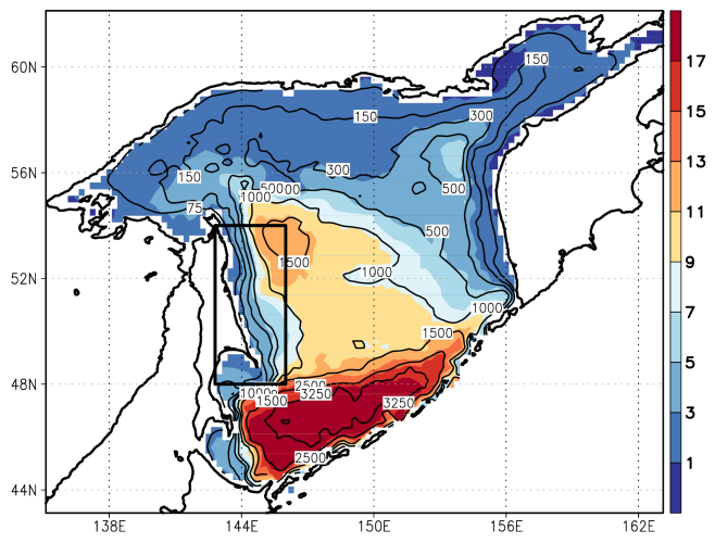
Figure 1: Annual mean first baroclinic Rossby radius of deformation in the Sea of Okhotsk (shading, km). Bottom topography of the Sea of Okhotsk extracted from the GEBCO dataset and smoothed by 9-point filter (lines, m). The rectangle marks out the region on the eastern Sakhalin Island (141.6^∘E–146^∘E, 44^∘N–55^∘N).

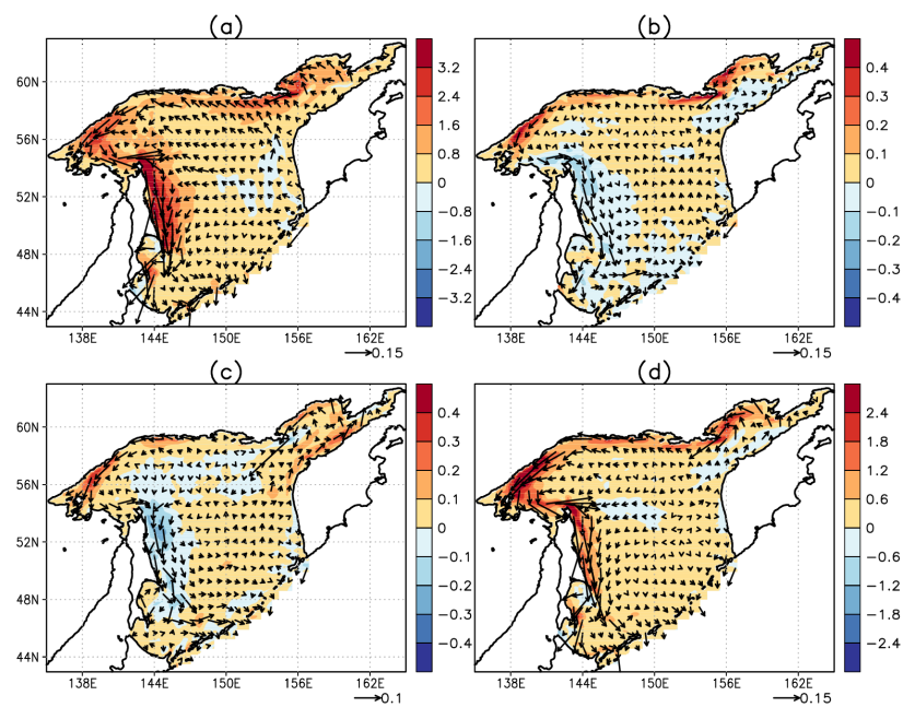
Figure 2: Seasonal mean wind power input (shading, 10^-2W m^-2) and velocity field at the horizon of 10 m (vectors, m s^-1) in (a) winter (January, February, March), (b) spring (April, May, June), (c) summer (July, August, September) and (d) autumn (October, November, December).

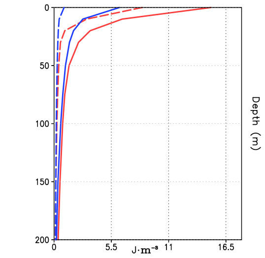
Figure 3: Basin-averaged vertical profiles of the EKE (red line) and MKE (blue line) over the Sea of Okhotsk in winter (January, February, and March) (dashed line) and summer (July, August and September) (solid line).

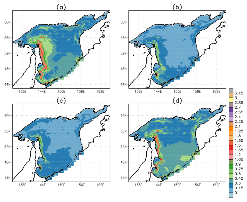
Figure 4: The mean EKE (10³ J m^-2) integrated in the upper 200 m in (a) winter, (b) spring, (c) summer and (d) autumn.

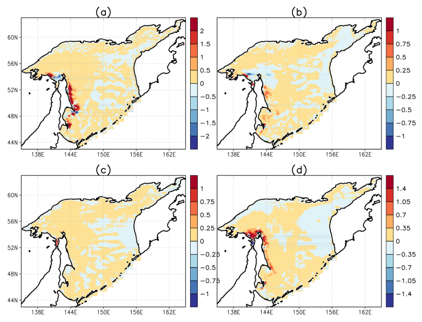
Figure 5: Distribution of the rate of the energy conversion term (BC) (10^-2 W m^-2) integrated in the upper 200 m in (a) winter, (b) spring, (c) summer and (d) autumn.

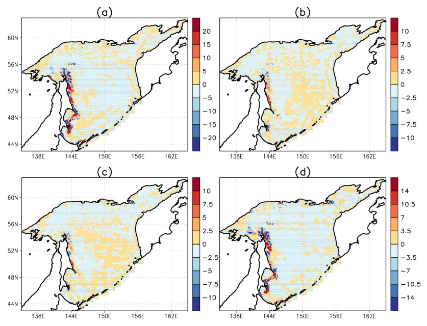
Figure 6: Distribution of the rate of the energy conversion term (BT) (10^-4 W m^-2) integrated in the upper 200 m in (a) winter, (b) spring, (c) summer and (d) autumn.

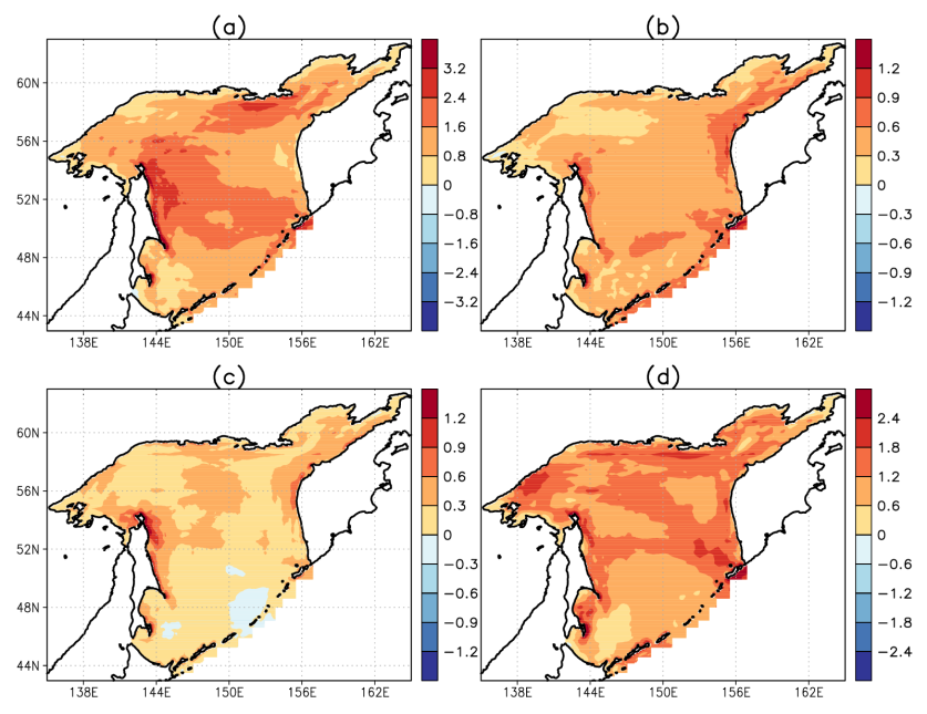
Figure 7: Distribution of generation of EKE due to time-varying wind stress (10^-2 W m^-2) in (a) winter, (b) spring, (c) summer and (d) autumn.

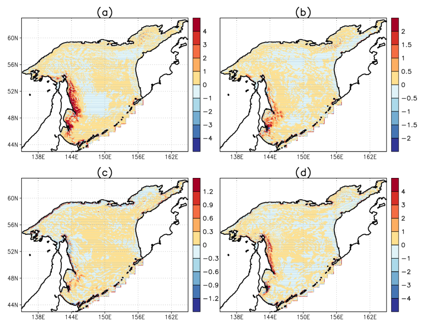
Figure 8: Distribution of the rate of energy conversion from EPE to EKE $(-\overline{\rho^{\prime}w^{\prime}}g)$ (10^-3 W m^-2) integrated in the upper 200 m in (a) winter, (b) spring, (c) summer and (d) autumn.

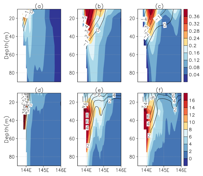
Figure 9: Vertical section of monthly mean meridional velocity (shedding, m s^-1) and density deviation (line, kg m^-3) from the reference value $\rho_{0}$, amounting to 1025 kg m^-3, across the eastern shelf of Sakhalin Island (50.46^∘N) in (a) January, (b) February and (c) March 2005. Left-hand side (lines, 10^-3 s^-1) and right-hand side (shading, 10^-3 s^-1) of relation (15) in: (d) January, (e) February, and (f) March 2005.

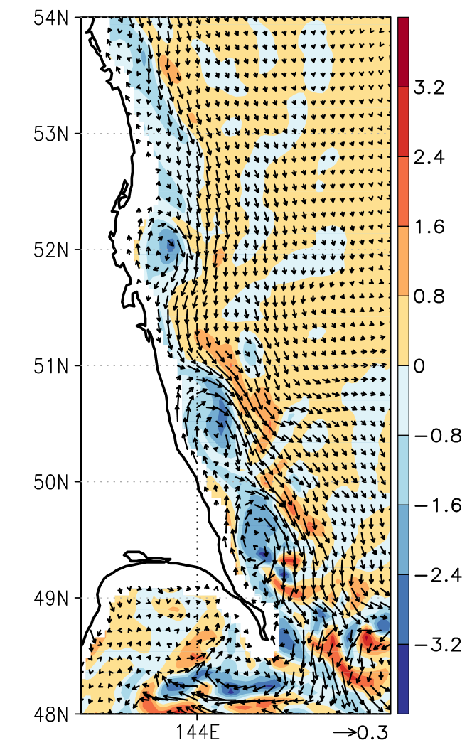
Figure 10: Velocity field (vectors, m s^-1) and vertical component of relative vorticity (shading, 10^-1) at the horizon of 20 m on the eastern shelf of Sakhalin Island on 8 April 2005.

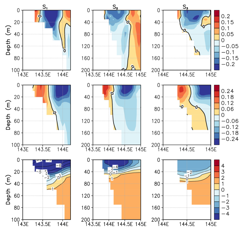
Figure 11: Vertical structure on the zonal sections: (143^∘E–144.2^∘E, 52^∘N) left column, (143.5^∘E–145^∘E, 50.46^∘N) central column and (144^∘E–145^∘E, 49.51^∘N) right column across the eastern shelf of Sakhalin Island on 8 April 2005: (a) vertical component of relative vorticity (shading), (b) meridional velocity (shading, m s^-1) and (c) density deviation (shading, kg m^-3) from the reference value $\rho_{0}$ amounts to 1025 kg m^-3

Table 1: Long-term mean rates of energy conversion (BT and BC) and magnitudes of two sources of the EKE ($\overline{\mathbf{\tau}^{\prime}\cdot\mathbf{u}^{\prime}_{s}}$ and $-\overline{\rho^{\prime}w^{\prime}g}$), integrated in the upper 200 m on the eastern shelf of Sakhalin Island (141.6^∘E–146^∘E, 44^∘N–55^∘N). Unit is in 10⁹W

Season	$BT=-\rho_{0}\overline{\mathbf{u}^{\prime}_{h}\cdot(\mathbf{u}^{\prime}\cdot\nabla\overline{\mathbf{u}_{h}})}$	$BC=-\frac{g^{2}}{\overline{N}^{2}\rho_{0}}\overline{\mathbf{u}^{\prime}_{h}\rho^{\prime}}\cdot\nabla_{h}\overline{\rho}$	$\overline{\mathbf{\tau}^{\prime}\cdot\mathbf{u}^{\prime}_{s}}$	$-\overline{\rho^{\prime}w^{\prime}g}$
$Winter$	$-4.2\cdot 10^{-3}$	0.9	4.0	0.3
$Spring$	$-2.7\cdot 10^{-3}$	0.1	1.2	$2\cdot 10^{-2}$
$Summer$	$-1.9\cdot 10^{-3}$	0.1	0.9	$-2.9\cdot 10^{-2}$
$Autumn$	$-2.1\cdot 10^{-3}$	0.5	2.9	$5.8\cdot 10^{-2}$