Smectic phases in ionic liquid crystals

Abstract

Ionic liquid crystals (ILCs) are anisotropic mesogenic molecules which carry charges and therefore combine properties of liquid crystals, e.g., the formation of mesophases, and of ionic liquids, such as low melting temperatures and tiny triple-point pressures. Previous density functional calculations have revealed that the phase behavior of ILCs is strongly affected by their molecular properties, i.e., their aspect ratio, the loci of the charges, and their interaction strengths. Here, we report new findings concerning the phase behavior of ILCs as obtained by density functional theory and Monte Carlo simulations. The most important result is the occurrence of a novel, wide smectic-A phase $S_{AW}$, at low temperature, the layer spacing of which is larger than that of the ordinary high-temperature smectic-A phase $S_{A}$. Unlike the ordinary smectic $S_{A}$ phase, the structure of the $S_{AW}$ phase consists of alternating layers of particles oriented parallel to the layer normal and oriented perpendicular to it.

I Introduction

Ionic liquid crystals (ILCs) Binnemans (2005); Kondrat et al. (2010) combine characteristics of liquid crystals and ionic liquids such as anisotropic material properties and ionic conductivity, respectively. They attract steadily growing scientific and technological interest. A common molecular structure of ILCs is that of charged imidazolium rings with highly anisotropic alkyl chains attached. Varying the length of the alkyl chains as well as the number and loci of the charged groups offers the possibility to optimize and tune material properties upon synthesis Binnemans (2005). For instance, ILCs forming either columnar or smectic phases can show a high conductivity in one dimension (parallel to the columnar stacks), respectively in two dimensions (perpendicular to the smectic layer normal). Therefore they can potentially be used as anisotropic electrolytes in batteries Yoshio et al. (2006); Bruce et al. (2008); Kato (2010). Moreover, ILCs can be synthesized such that they exhibit high thermal as well as mechanical stability Binnemans (2005); Goossens et al. (2016). The combination of (low-dimensional) high conductivity and durability renders ILCs promising candidates as electrolyte constituents, e.g., in solar cells Yamanaka et al. (2005, 2007). Additionally, since ILCs can be regarded as anisotropic solvents, they can also be used as organized reaction media Lee et al. (2000); Goossens et al. (2016) which, due to their nanostructure, facilitate chemical reactions or offer a higher degree of control over the reactions.

Another, but closely related, class of liquids are room temperature ionic liquids (RTILs) which at ambient pressure exhibit a melting temperature below room temperature. For these materials, as well as for ILCs, it is the combination of molecular shape-anisotropy and the presence of charges which leads to a variety of astonishing properties of these fluids. Besides the remarkable low melting temperature of RTILs, caused by a suppression of crystallization at room temperature (due to the underlying molecular shape-anisotropy), RTILs show an almost negligible vapor pressure which renders them candidates as solvents for ultrahigh vacuum applications Liu et al. (2002); Wang et al. (2004); Suzuki et al. (2007); Bermúdez et al. (2009); Bier and Dietrich (2010). The notion room temperature ionic liquid emphasizes that this class of material remains liquid at standard conditions. But, on one hand, RTILs may in addition exhibit liquid crystalline phases (below room temperature), which renders these room temperature ionic liquids also ionic liquid crystals. On the other hand, if the molecular structure of RTILs is sufficiently asymmetric, no liquid-crystalline orientational ordering can be established and thus no mesophases will occur, which distinguishes this kind of RTILs from ILCs.

The technological use of ILCs and RTILs requires an in-depth understanding of the microscopical mechanisms, in particular the interplay of molecular shape-anisotropy and the presence of charges, leading to the remarkable behaviors of those materials. Thus, theoretical studies, which incorporate anisotropic charged particles and which allow one to vary molecular properties (e.g., by tuning the aspect-ratio or the charge distribution of the underlying particles), might elucidate the role these microscopic properties play for the above mentioned remarkable macroscopic features of both classes of fluids, ILCs and RTILs.

On the one hand, previous theoretical studies mainly focused either on the effect of molecular shape-anisotropy on thermodynamic properties or on ionic liquids within simplistic models. For instance, the restricted primitive model (RPM), for which both ion species are considered to be uniformly charged hard spheres of the same size and the same charge strength, has been studied intensively in the past, both in the continuum Stell et al. (1976); Gillan (1983) as well as on lattices Dickman and Stell (1999); Panagiotopoulos and Kumar (1999); Bartsch et al. (2015). However, models incorporating spherically-shaped ions are designed to study gross features such as the nature of criticality Fisher (1994); Caillol et al. (1997); Orkoulas and Panagiotopoulos (1999); Dickman and Stell (1999); Panagiotopoulos and Kumar (1999); Panagiotopoulos (2002).

On the other hand, there is a vast number of theoretical studies concerning ordinary (uncharged) liquid crystals, which are based on the elongated shapes of the underlying molecules and their anisotropic pair potentials Onsager (1949); Maier and Saupe (1958, 1959, 1960); McMillan (1971, 1972); Straley (1971, 1973, 1976); Sheng and Wojtowicz (1976). Depending on the effective shape of the particles and their interaction potentials one observes a huge diversity of mesophases – phases in between the isotropic liquid and the crystalline phase distinguishable by their degree of positional and orientational ordering – occurring in systems of liquid crystals. While plate-like particles (discotic mesogenes) at high densities tend to form columnar phases, in which the particles form stack-like structures, in dense systems of elongated particles, like thin rods or prolate ellipsoids (calamitic mesogens) one typically observes smectic structures, in which the particles are located in layers de Gennes (1974). (We note that although the formation of a columnar phase in a binary mixture of hard spherocylinders has been reported Stroobants (1992), this phase is not formed in a monodisperse system.) This distinct behavior due to the molecular anisotropy gives rise to macroscopically measurable optical and mechanical anisotropies of liquid-crystalline materials and drives phenomena like self-assembly or nano-structuring on microscopic scales Kato et al. (2006); Goodby et al. (2008); Tschierske (2013).

It is the very interplay of shape-anisotropy and electrostatic interactions, which gives rise to the vast phenomenology observed for ILC materials and at the same time poses a particular challenge for theoretical studies. Establishing a theoretical framework, which is applicable to this kind of materials and allows one to gain a deeper understanding of the origin of their properties, is an ongoing process. Recently, Goossens et al. Goossens et al. (2016) discussed in their review article the latest developments in synthesis, characterization, and applications of ILCs. In particular, they concluded that a deeper understanding of the role of the size, the shape, and the charge distribution of the ILC molecules for the properties of those materials is required. The aim of the present contribution is to show that the considered molecular model of an ionic fluid, incorporating orientational degrees of freedom as well as an anisotropic charge distribution, gives rise to a phenomenology concerning the phase behavior and the structural properties of the bulk phases, which is much richer than the one of simpler models of spherical ions or of ordinary liquid crystals. The most important new result is the occurrence of a novel smectic phase $S_{AW}$ at low temperatures, the layer spacing of which is larger than that of the ordinary high-temperature smectic phase $S_{A}$. The present findings stress the crucial role of the loci of the charges on the ILC molecules and at the same time emphasize the necessity of considering such kind of sophisticated model in order to study reliably complex ionic liquids such as room temperature ionic liquids.

The present study is structured as follows: In Sec. II the employed model is presented as well as the outlines of the methods which encompass density functional theory and Monte Carlo simulations. Our results for the phase behavior and for the structure of various smectic phases of ILCs are discussed in Sec. III. Finally, in Sec. IV we summarize the results and draw our conclusions.

II Model and methods

This section presents in detail the molecular model of ILCs as employed here. In particular, we discuss the intermolecular pair potential, which can be applied to a wide range of ionic and liquid crystalline materials due to its flexibility provided by a large set of parameters.

This model is studied by density functional theory (DFT) as well as by grandcanonical Monte Carlo simulations. The methodological and technical details of both approaches are described in Secs. II.2 and II.3, respectively.

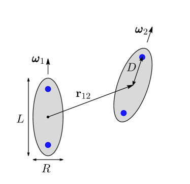
Figure 1: Cross-sectional view of two ILC molecules in the plane spanned by the orientations $\boldsymbol{\omega}_{i},~{}i=1,2$, of their long axis. The particles are treated as rigid prolate ellipsoids, characterized by their length-to-breadth ratio $L/R$. Their orientations are fully described by the direction of their long axis $\boldsymbol{\omega}_{i}$; $\boldsymbol{r}_{12}$ is the center-to-center distance vector. The charges of the ILC molecules (blue dots) are located on the long axis at a distance $D$ from their geometrical center. The counterions are not modeled explicitly, but they are implicitly accounted for in terms of a background, giving rise to the screening of the charges of the ILC molecules.

II.1 Molecular model and pair potential

We consider a coarse-grained description of the ILC molecules as rigid prolate ellipsoids of length-to-breadth ratio $L/R$ (see Fig. 1). Thus, the orientation of a molecule is fully described by the direction $\boldsymbol{\omega}(\phi,\vartheta)$ of its long axis, where $\phi$ and $\vartheta$ denote the azimuthal and polar angle, respectively.

The two-body interaction potential consists of a hard core repulsive and an additional contribution $U_{\text{GB}}+U_{\text{es}}$ beyond the contact distance $R\sigma$, the sum of which can be attractive or repulsive:

$$U=\begin{cases}\infty&,|\boldsymbol{r}_{12}|<R\sigma(\boldsymbol{\hat{r}}_{12},\boldsymbol{\omega}_{1},\boldsymbol{\omega}_{2})\\ \begin{array}[]{l}U_{\text{GB}}(\boldsymbol{r}_{12},\boldsymbol{\omega}_{1},\boldsymbol{\omega}_{2})+\\ U_{\text{es}}(\boldsymbol{r}_{12},\boldsymbol{\omega}_{1},\boldsymbol{\omega}_{2})\end{array}&,|\boldsymbol{r}_{12}|\geq R\sigma(\boldsymbol{\hat{r}}_{12},\boldsymbol{\omega}_{1},\boldsymbol{\omega}_{2}),\end{cases}$$ (1)

where $\boldsymbol{r}_{12}:=\boldsymbol{r}_{2}-\boldsymbol{r}_{1}$ denotes the center-to-center distance vector between the two particles labeled as 1 and 2, and $\boldsymbol{\omega}_{i}$, $i=1,2$, are their orientations. The contact distance $R\sigma(\boldsymbol{\hat{r}}_{12},\boldsymbol{\omega}_{1},\boldsymbol{\omega}_{2})$ depends on the orientations of both particles and their relative direction, which is expressed by the unit vector $\boldsymbol{\hat{r}}_{12}:=\boldsymbol{r}_{12}/|\boldsymbol{r}_{12}|$. In Eq. (1), we subdivided the contributions beyond the contact distance $|\boldsymbol{r}_{12}|\geq R\sigma$ into two parts: $U_{\text{GB}}(\boldsymbol{r}_{12},\boldsymbol{\omega}_{1},\boldsymbol{\omega}_{2})$ is the well-known Gay-Berne potential Berne and Pechukas (1972); Gay and Berne (1981), which incorporates an attractive van der Waals-like interaction between molecules and which can be understood as a generalization of the Lennard-Jones pair potential to ellipsoidal particles:

$$\begin{split}&U_{\text{GB}}(\boldsymbol{r}_{12},\boldsymbol{\omega}_{1},\boldsymbol{\omega}_{2})=4\varepsilon(\boldsymbol{\hat{r}}_{12},\boldsymbol{\omega}_{1},\boldsymbol{\omega}_{2})\\ &\times\left[\left(1+\frac{|\boldsymbol{r}_{12}|}{R}-\sigma(\boldsymbol{\hat{r}}_{12},\boldsymbol{\omega}_{1},\boldsymbol{\omega}_{2})\right)^{-12}\right.\\ &\left.-~{}\left(1+\frac{|\boldsymbol{r}_{12}|}{R}-\sigma(\boldsymbol{\hat{r}}_{12},\boldsymbol{\omega}_{1},\boldsymbol{\omega}_{2})\right)^{-6}\right]\\ \end{split}$$ (2)

with

$$\begin{split}\sigma(\boldsymbol{\hat{r}}_{12},\boldsymbol{\omega}_{1},\boldsymbol{\omega}_{2})&=\left[1-\frac{\chi}{2}\left(\frac{(\boldsymbol{\hat{r}}_{12}\cdot(\boldsymbol{\omega}_{1}+\boldsymbol{\omega}_{2}))^{2}}{1+\chi\boldsymbol{\omega}_{1}\cdot\boldsymbol{\omega}_{2}}\right.\right.\\ &\left.+\left.\frac{(\boldsymbol{\hat{r}}_{12}\cdot(\boldsymbol{\omega}_{1}-\boldsymbol{\omega}_{2}))^{2}}{1-\chi\boldsymbol{\omega}_{1}\cdot\boldsymbol{\omega}_{2}}\right)\right]\\ \end{split}$$ (3)

and

$$\begin{split}\varepsilon(\boldsymbol{\hat{r}}_{12},\boldsymbol{\omega}_{1},\boldsymbol{\omega}_{2})&=\varepsilon_{0}\left(1-(\chi\boldsymbol{\omega}_{1}\cdot\boldsymbol{\omega}_{2})^{2}\right)^{-1/2}\\ &\times\left[1-\frac{\chi^{\prime}}{2}\left(\frac{(\boldsymbol{\hat{r}}_{12}\cdot(\boldsymbol{\omega}_{1}+\boldsymbol{\omega}_{2}))^{2}}{1+\chi^{\prime}\boldsymbol{\omega}_{1}\cdot\boldsymbol{\omega}_{2}}\right.\right.\\ &\left.+\left.\frac{(\boldsymbol{\hat{r}}_{12}\cdot(\boldsymbol{\omega}_{1}-\boldsymbol{\omega}_{2}))^{2}}{1-\chi^{\prime}\boldsymbol{\omega}_{1}\cdot\boldsymbol{\omega}_{2}}\right)\right].\\ \end{split}$$ (4)

The contact distance $R\sigma(\boldsymbol{\hat{r}}_{12},\boldsymbol{\omega}_{1},\boldsymbol{\omega}_{2})$ and the direction- and orientation-dependent interaction strength $\varepsilon(\boldsymbol{\hat{r}}_{12},\boldsymbol{\omega}_{1},\boldsymbol{\omega}_{2})$ are both parametrically dependent on the length-to-breadth ratio $L/R$ via the auxiliary function $\chi=((L/R)^{2}-1)/((L/R)^{2}+1)$. Additionally, $\varepsilon(\boldsymbol{\hat{r}}_{12},\boldsymbol{\omega}_{1},\boldsymbol{\omega}_{2})$ can be tuned via $\chi^{\prime}=((\varepsilon_{R}/\varepsilon_{L})^{1/2}-1)/((\varepsilon_{R}/\varepsilon_{L})^{1/2}+1)$, where $\varepsilon_{R}/\varepsilon_{L}$ is called the anisotropy parameter, defined in terms of the ratio of $\varepsilon_{R}$, which is the depth of the potential minimum for parallel particles positioned side by side $(\boldsymbol{\hat{r}}_{12}\cdot\boldsymbol{\omega}_{1}=\boldsymbol{\hat{r}}_{12}\cdot\boldsymbol{\omega}_{2}=0)$, and $\varepsilon_{L}$, which is the depth of the potential minimum for parallel particles positioned end to end $(\boldsymbol{\hat{r}}_{12}\cdot\boldsymbol{\omega}_{1}=\boldsymbol{\hat{r}}_{12}\cdot\boldsymbol{\omega}_{2}=1)$. The energy scale of the Gay-Berne pair interaction is set by $\varepsilon_{0}$. Thus, the Gay-Berne pair potential has four independent free parameters: $\varepsilon_{0},R,L/R$, and $\varepsilon_{R}/\varepsilon_{L}$. Note that in the case of spherical particles, i.e., for $L=R$, the Gay-Berne pair potential (Eq. (2)) reduces to the well-known isotropic Lennard-Jones pair potential iff, additionally, the Gay-Berne anisotropy parameter equals unity, i.e., $\varepsilon_{R}/\varepsilon_{L}=1$, because then $\sigma(\boldsymbol{\hat{r}}_{12},\boldsymbol{\omega}_{1},\omega_{2})=1$ and $\varepsilon(\boldsymbol{\hat{r}}_{12},\boldsymbol{\omega}_{1},\omega_{2})=\varepsilon_{0}$.

The second contribution $U_{\text{es}}(\boldsymbol{r}_{12},\boldsymbol{\omega}_{1},\boldsymbol{\omega}_{2})$ in Eq. (1) is the electrostatic repulsion of ILC molecules. Within the scope of the present study, the counterions are not modeled explicitly, but they will be considered to be much smaller in size than the ILC molecules such that they can be treated as a continuous background. On the level of linear response, this background gives rise to the screening of the pure Coulomb potential between two charged sites on a length scale given by the Debye screening length $\lambda_{D}$ such that the effective electrostatic interaction of the ILC molecules is given by

$$\begin{split}U_{\text{es}}(\boldsymbol{r}_{12},\boldsymbol{\omega}_{1},\boldsymbol{\omega}_{2})=~{}&\gamma\left[\frac{\exp\left(-\frac{|\boldsymbol{r}_{12}+D(\boldsymbol{\omega}_{1}+\boldsymbol{\omega}_{2})|}{\lambda_{D}}\right)}{|\boldsymbol{r}_{12}+D(\boldsymbol{\omega}_{1}+\boldsymbol{\omega}_{2})|}\right.\\ &+\left.\frac{\exp\left(-\frac{|\boldsymbol{r}_{12}+D(\boldsymbol{\omega}_{1}-\boldsymbol{\omega}_{2})|}{\lambda_{D}}\right)}{|\boldsymbol{r}_{12}+D(\boldsymbol{\omega}_{1}-\boldsymbol{\omega}_{2})|}\right.\\ &+\left.\frac{\exp\left(-\frac{|\boldsymbol{r}_{12}-D(\boldsymbol{\omega}_{1}+\boldsymbol{\omega}_{2})|}{\lambda_{D}}\right)}{|\boldsymbol{r}_{12}-D(\boldsymbol{\omega}_{1}+\boldsymbol{\omega}_{2})|}\right.\\ &+\left.\frac{\exp\left(-\frac{|\boldsymbol{r}_{12}-D(\boldsymbol{\omega}_{1}-\boldsymbol{\omega}_{2})|}{\lambda_{D}}\right)}{|\boldsymbol{r}_{12}-D(\boldsymbol{\omega}_{1}-\boldsymbol{\omega}_{2})|}\right].\end{split}$$ (5)

The charges $q$ are located symmetrically on their long axis at a distance $D$ from the geometrical center of the particles (compare Fig. 1); $\gamma=q^{2}/(4\pi\varepsilon)$ characterizes the electrostatic energy scale with permittivity $\varepsilon$. In principle, the Debye screening length

$$\lambda_{D}=\sqrt{\frac{kT}{q^{2}\varrho_{\text{c}}}}$$ (6)

is a function of temperature $T$ and of the number density $\varrho_{\text{c}}$ of the counter ions. Thus, it depends on the thermodynamic state of the fluid. However, in the present model $\lambda_{D}$ is taken to be a constant parameter. In order to compare results, obtained within this model, with data from actual physical systems, one could measure the value of the Debye screening length experimentally and tune the model parameter $\lambda_{D}$ accordingly.

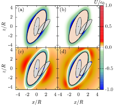
Figure 2: Contour-plots of the pair potential $U$ for $|\boldsymbol{r}_{12}|\geq R\sigma$ in the $x$-$z$-plane for four cases of particles with fixed length-to-breadth ratio $L/R=4$ and fixed orientations. In each panel the centers of both particles lie in the plane $y=0$. In order to illustrate the orientations of the ellipsoids, they have been included in the plots at contact with relative direction $\boldsymbol{\hat{r}}_{12}=\boldsymbol{\hat{x}}$. The set of points at contact in the $x$-$z$-plane is illustrated by the black curve and the centers of the particles are shown by small black dots. Panel (a): uncharged liquid crystal with $\varepsilon_{R}/\varepsilon_{L}=2$. Panel (b): uncharged liquid crystal with $\varepsilon_{R}/\varepsilon_{L}=4$. The anisotropy of the potential is increased slightly. Panel (c): ILC with $\varepsilon_{R}/\varepsilon_{L}=2,D/R=0,\lambda_{D}/R=5,\gamma/(R\varepsilon_{0})=0.25$. Panel (d): ILC with $\varepsilon_{R}/\varepsilon_{L}={\color[rgb]{0,0,0}2},D/R=1.8,\lambda_{D}/R=5,\gamma/(R\varepsilon_{0})=0.25$. In (c) and (d) the loci of the charges are indicated as blue dots. The salmon-colored area is the excluded volume for given orientations of the two particles.

In Fig. 2 we illustrate the full pair potential (Eq. (1)) beyond the contact distance for certain choices of the parameters. The two top panels, (a) and (b), show the pure Gay-Berne potential (uncharged liquid crystals), which is predominantly attractive in the space outside the overlap volume (cream-colored area). The shape of the overlap volume changes by varying the particle orientations as well as by changing the length-to-breadth ratio $L/R$. However, these dependences are not apparent from Fig. 2, since $L/R=4$ and the particle orientations $\boldsymbol{\omega}_{i}$ are kept fixed for all panels. In panel (b) the anisotropy parameter $\varepsilon_{R}/\varepsilon_{L}=4$ is chosen to be two times larger than for panel (a) ($\varepsilon_{R}/\varepsilon_{L}=2$). Thus, the ratio of the well depth at the tails and at the sides is increased. The two bottom panels, (c) and (d), show the same choices for the Gay-Berne parameters as for panel (a), but the electrostatic repulsion of the charged groups on the molecules, illustrated by blue dots, is included ($\gamma/(R\varepsilon_{0})=0.25$). In panel (c) the loci of the two charges of the particles coincide at its center (i.e., $D/R=0$) while in panel (d) they are located near the tips ($D/R=1.8$). For both cases with charge, the effective interaction range is significantly increased compared with the uncharged case and is governed by the Debye screening length, chosen as $\lambda_{D}/R=5$.

II.2 Density functional theory

II.2.1 Formalism

The degrees of freedom of the particles (compare Sec. II.1) are fully described by the positions $\boldsymbol{r}$ of their centers and the orientations $\boldsymbol{\omega}$ of their long axes. Thus, within density functional theory an appropriate variational grand potential functional $\beta\Omega[\varrho]$ of position- and orientation-dependent number density profiles $\varrho(\boldsymbol{r},\boldsymbol{\omega})$ has to be found; its minimum corresponds to the equilibrium density profile. The grand potential functional for uniaxial particles, in the absence of external fields, can generically be expressed as

$$\begin{split}\beta\Omega\left[\varrho\right]=&\int_{\mathcal{V}}\!\mathrm{d}^{3}{r}\;\int_{\mathcal{S}}\!\mathrm{d}^{2}{\omega}\;\varrho(\boldsymbol{r},\boldsymbol{\omega})\left[\ln\left(4\pi\Lambda^{3}\varrho(\boldsymbol{r},\boldsymbol{\omega})\right)\right.\\ &-\left.\left(1+\beta\mu\right)\right]+\beta\mathcal{F}\left[\varrho\right],\end{split}$$ (7)

where the integration domains $\mathcal{V}$ and $\mathcal{S}$ denote the system volume and the full solid angle, respectively. The first term in Eq. (7) is the purely entropic free energy contribution of non-interacting uniaxial particles, where $\beta=1/(k_{B}T)$ denotes the inverse thermal energy, $\mu$ the chemical potential, and $\Lambda$ the thermal de Broglie wavelength. The last term is the excess free energy $\beta\mathcal{F}\left[\varrho\right]$ in units of $k_{B}T$, which incorporates the effects of the inter-particle interactions. Minimizing Eq. (7) leads to the Euler-Lagrange equation, which implicitly determines the equilibrium density profile $\varrho(\boldsymbol{r},\boldsymbol{\omega})$:

$$\varrho(\boldsymbol{r},\boldsymbol{\omega})=\frac{e^{\beta\mu}}{4\pi\Lambda^{3}}\exp\left[c^{(1)}\left(\boldsymbol{r},\boldsymbol{\omega},[\varrho]\right)\right],$$ (8)

where

$$c^{(1)}\left(\boldsymbol{r},\boldsymbol{\omega},[\varrho]\right)=-\frac{\delta\beta\mathcal{F}[\varrho]}{\delta\varrho}$$ (9)

is the one-particle direct correlation function. It is fully determined by the excess free energy functional $\beta\mathcal{F}[\varrho]$.

Since the excess free energy functional is the characterizing quantity of the underlying many-body problem, in general it is not known exactly so that one has to find appropriate approximations of it. The starting point of the present study is a weighted density formulation of $\beta\mathcal{F}[\varrho]$ in the spirit of Ref. Tarazona (1985):

$$\beta\mathcal{F}[\varrho]=\frac{1}{2}\int_{\mathcal{V}}\!\mathrm{d}^{3}{r}\;\int_{\mathcal{S}}\!\mathrm{d}^{2}{\omega}\;\varrho(\boldsymbol{r},\boldsymbol{\omega})\beta\psi\left(\boldsymbol{r},\boldsymbol{\omega},[\bar{\varrho}]\right),$$ (10)

which immediately leads to the following expression for the one-particle direct correlation function:

$$c^{(1)}\left(\boldsymbol{r},\boldsymbol{\omega},[\varrho]\right)=-\frac{1}{2}\bigg{[}\beta\psi(\boldsymbol{r},\boldsymbol{\omega},[\bar{\varrho}])+\int_{\mathcal{V}}\!\mathrm{d}^{3}{r^{\prime}}\;\int_{\mathcal{S}}\!\mathrm{d}^{2}{\omega^{\prime}}\;\varrho(\boldsymbol{r}^{\prime},\boldsymbol{\omega}^{\prime})$$

$$\times\int_{\mathcal{V}}\!\mathrm{d}^{3}{r^{\prime\prime}}\;\int_{\mathcal{S}}\!\mathrm{d}^{2}{\omega^{\prime\prime}}\;\frac{\delta\beta\psi(\boldsymbol{r}^{\prime},\boldsymbol{\omega}^{\prime},[\bar{\varrho}])}{\delta\bar{\varrho}(\boldsymbol{r}^{\prime\prime},\boldsymbol{\omega}^{\prime\prime})}\,\frac{\delta\bar{\varrho}(\boldsymbol{r}^{\prime\prime},\boldsymbol{\omega}^{\prime\prime},[\varrho])}{\delta\varrho(\boldsymbol{r},\boldsymbol{\omega})}\bigg{]}.$$ (11)

In order to evaluate Eq. (11), one needs to know the effective one-particle potential $\beta\psi[\bar{\varrho}]$ as a functional of the weighted density $\bar{\varrho}(\boldsymbol{r},\boldsymbol{\omega},[\varrho])$, which in the present case is chosen as a projection of the full density profile $\varrho(\boldsymbol{r},\boldsymbol{\omega})$ onto a certain functional subspace (see below).

The present work aims at studying the phase behavior of ILCs, composed of uniaxial prolate particles. Hence, one expects the occurrence of isotropic (no positional and no orientational order), nematic (no positional, but orientational order), and smectic phases (one-dimensional positional order in $z$-direction and orientational order). At sufficiently low temperatures and sufficiently large densities the homogenous phases mentioned above, i.e., the isotropic and nematic phases, or partially homogenous phases, i.e., the smectic phases, undergo transitions to crystalline phases. The first three types of phases can be represented by spatially periodic density profiles $\varrho(\boldsymbol{r},\boldsymbol{\omega})$ with wavelength $d$ in $z$-direction and spatially constant density perpendicular to it. For a uniform density in $z$-direction $d$ is not uniquely defined and can be chosen arbitrarily, whereas for smectic structures with layers perpendicular to the $z$-direction $d$ is an integer multiple of the layer spacing. (Although there is no need to introduce $d$ for uniform phases, within the present approach based on the projected density $\bar{\varrho}(\boldsymbol{r},\boldsymbol{\omega})$ (see Eqs. (12)-(14) below), also a uniform density profile $\varrho(\boldsymbol{r},\boldsymbol{\omega})$ demands a value for $d$ entering into Eq. (14). However, the corresponding results do not depend on such a choice of $d$; any value $d>0$ is valid.) This observation motivates the approach to consider a projected density $\bar{\varrho}(\boldsymbol{r},\boldsymbol{\omega},[\varrho])$, which is obtained by weighting the original density profile $\varrho(\boldsymbol{r},\boldsymbol{\omega})$ within a periodic cell of volume $\mathcal{V}_{d}=A\times d$ around the position $\boldsymbol{r}$, where $A$ is the cross-sectional area of the system. In order to express the orientational dependence of the projected density $\bar{\varrho}(\boldsymbol{r},\boldsymbol{\omega})$ explicitly, in addition to the Fourier series expansion of $\varrho(\boldsymbol{r},\boldsymbol{\omega})$ in terms of $\cos(2\pi iz/d)$ (with $i=0,1,2$) $\bar{\varrho}(\boldsymbol{r},\boldsymbol{\omega})$ (Eq. (12)) is determined by performing furthermore an expansion of $\varrho(\boldsymbol{r},\boldsymbol{\omega})$ in terms of Legendre polynomials $P_{l}(y=\cos\vartheta)$ up to and including second order, i.e., $l=0,2$. The contribution corresponding to $l=1$ vanishes due to the symmetry of the underlying pair potential $U(\boldsymbol{r}_{12},\boldsymbol{\omega}_{1},\boldsymbol{\omega}_{2})$ (Eq. (1)):

$$\begin{split}&\bar{\varrho}(\boldsymbol{r},\boldsymbol{\omega},[\varrho])=\frac{1}{4\pi}\bigg{[}Q_{0}(\boldsymbol{r},[\varrho])+Q_{1}(\boldsymbol{r},[\varrho])\cos\left(2\pi z/d\right)\\ &+Q_{2}(\boldsymbol{r},[\varrho])\cos\left(4\pi z/d\right)+5P_{2}(\cos(\vartheta))\bigg{(}Q_{3}(\boldsymbol{r},[\varrho])\\ &+Q_{4}(\boldsymbol{r},[\varrho])\cos\left(2\pi z/d\right)+Q_{5}(\boldsymbol{r},[\varrho])\cos\left(4\pi z/d\right)\bigg{)}\bigg{]},\end{split}$$ (12)

where $P_{0}(y)=1$, $P_{2}(y)=(3y^{2}-1)/2$, and with coefficients $Q_{i}(\boldsymbol{r},[\varrho])$ defined as

$$Q_{i}(\boldsymbol{r},[\varrho]) =\frac{1}{\mathcal{V}_{d}}\int_{\mathcal{V}}\!\mathrm{d}^{3}{r^{\prime}}\;\int_{\mathcal{S}}\!\mathrm{d}^{2}{\omega^{\prime}}\;\varrho(\boldsymbol{r}^{\prime},\boldsymbol{\omega}^{\prime})w_{i}(z,z^{\prime},\vartheta^{\prime})$$ (13)

with

$$w_{0} =\Theta(d/2-|z-z^{\prime}|),$$

$$w_{1} =2\Theta(d/2-|z-z^{\prime}|)\cos\left(2\pi z^{\prime}/d\right),$$

$$w_{2} =2\Theta(d/2-|z-z^{\prime}|)\cos\left(4\pi z^{\prime}/d\right),$$

$$w_{3} =\Theta(d/2-|z-z^{\prime}|)P_{2}(\cos(\vartheta^{\prime})),$$

$$w_{4} =2\Theta(d/2-|z-z^{\prime}|)P_{2}(\cos(\vartheta^{\prime}))\cos\left(2\pi z^{\prime}/d\right),$$

$$w_{5} =2\Theta(d/2-|z-z^{\prime}|)P_{2}(\cos(\vartheta^{\prime}))\cos\left(4\pi z^{\prime}/d\right).$$ (14)

Here $\Theta(x)$ denotes the Heaviside step function; concerning $\vartheta$ see below. Without loss of generality, for the three relevant bulk phases one can consider the entire system being composed of a set of periodic macro-cells.

Although in general the coefficients $Q_{i}(\boldsymbol{r},[\varrho])$ depend on the position $\boldsymbol{r}$, e.g., close to interfaces, for the scope of the present study they are constant, $Q_{i}(\boldsymbol{r},[\varrho])=Q_{i}=\text{const}$, because here we consider spatially periodic bulk profiles only. Thus, the coefficients $Q_{i}$ in Eqs. (13) and (14) represent the first coefficients of a Fourier expansion of the spatially periodic function $\varrho(\boldsymbol{r},\boldsymbol{\omega})$. Note, that the factor $2$ for $w_{1}$, $w_{2}$, $w_{4}$, and $w_{5}$ in Eq. (14) is due to the definition of the first and second Fourier modes. Similarly, the factor $5$ in the last term of Eq. (12) is due to the definition of the coefficient of the second order term of an expansion in terms of Legendre polynomials. The normal of the smectic layers is chosen to be parallel to the $z$-axis. We restrict our analysis of smectic phases to the case in which the director field $\boldsymbol{\hat{n}}(\boldsymbol{r})=\boldsymbol{\hat{z}}$, describing the mean orientation of the particles, is homogenous and points along the $z$-direction as well (smectic-A ($S_{A}$) de Gennes (1974)). Additionally, only distributions of orientations $\boldsymbol{\omega}$, which are symmetric around the director $\boldsymbol{\hat{n}}$, are considered, with the polar angle $\vartheta$ between the director and the long-axis of one particle is given by $\cos(\vartheta):=\boldsymbol{\hat{n}}\cdot\boldsymbol{\omega}$. Thus, our description is restricted to uniaxial phases, like the isotropic, nematic, and the smectic-A phase considered here. In order to study biaxial phases (e.g., smectic-C phases where the director is tilted with respect to the layer normal) within the present DFT-approach one would need to keep the full orientational dependence of the projected density $\bar{\varrho}(\boldsymbol{r},\boldsymbol{\omega})$ on both the polar angle $\vartheta$ and the azimuthal angle $\phi$. However, the present computer simulations did not reveal any evidence of the occurrence of biaxial phases in the investigated systems. In particular, the smectic-A-type phases were the only smectic phases that could be observed (see Sec. III). Therefore, the restriction to uniaxial structures seems to be adequate for the systems studied here.

In the final step of constructing the density functional, the effective one-particle potential $\beta\psi[\bar{\varrho}]$ needs to be specified. Here, it consists of two contributions. The first one is due to the hard-core interaction. For this contribution we adopt the well-studied Parsons-Lee approach Parsons (1979); Lee (1987)

$$\beta\psi_{\text{PL}}(\boldsymbol{r},\boldsymbol{\omega},[\bar{\varrho}])={\color[rgb]{0,0,0}-}\int_{\mathcal{V}}\!\mathrm{d}^{3}{r^{\prime}}\;\int_{\mathcal{S}}\!\mathrm{d}^{2}{\omega^{\prime}}\;\bar{\varrho}(\boldsymbol{r}^{\prime},\boldsymbol{\omega}^{\prime})$$

$$\times\frac{\mathcal{J}(Q_{0}(\boldsymbol{r}))+\mathcal{J}(Q_{0}(\boldsymbol{r}^{\prime}))}{2}f_{M}(\boldsymbol{r}-\boldsymbol{r}^{\prime},\boldsymbol{\omega},\boldsymbol{\omega}^{\prime}),$$ (15)

where $f_{M}(\boldsymbol{r}-\boldsymbol{r}^{\prime},\boldsymbol{\omega},\boldsymbol{\omega}^{\prime})$ is the Mayer f-function Hansen and McDonald (1986) of the hard core pair interaction potential and $\mathcal{J}(Q_{0})$ modifies the corresponding original Onsager free energy functional (i.e., the second-order virial approximation) such that the Carnahan-Starling equation of state Lee (1987) is reproduced for spheres, i.e., $L=R$ Onsager (1949); van Roij (2005):

$$\mathcal{J}(Q_{0})=\frac{1-\frac{3}{4}\eta_{0}(Q_{0})}{(1-\eta_{0}(Q_{0}))^{2}},$$ (16)

where $\eta_{0}=Q_{0}\,LR^{2}\pi/6$ denotes the mean packing fraction within the volume $\mathcal{V}_{d}$. It is proportional to the coefficient $Q_{0}$ which gives the mean density within the volume $\mathcal{V}_{d}$. The original Onsager functional is recovered by replacing $\mathcal{J}(Q_{0})$ by $Q_{0}$ in Eq. (15).

The second contribution to the effective one-particle potential $\beta\psi[\bar{\varrho}]$ takes into account the interactions beyond the contact distance (see the case $|\boldsymbol{r}_{12}|\geq R\sigma$ in Eq. (1)) within the modified mean-field approximation Teixeira and da Gama (1991), a variant of the extended random phase approximation (ERPA) Evans (1979):

$$\beta\psi_{\text{ERPA}}(\boldsymbol{r},\boldsymbol{\omega},[\bar{\varrho}])=\int_{\mathcal{V}}\!\mathrm{d}^{3}{r^{\prime}}\;\int_{\mathcal{S}}\!\mathrm{d}^{2}{\omega^{\prime}}\;\bar{\varrho}(\boldsymbol{r}^{\prime},\boldsymbol{\omega}^{\prime})$$

$$\times\beta U(\boldsymbol{r}-\boldsymbol{r}^{\prime},\boldsymbol{\omega},\boldsymbol{\omega}^{\prime})(1+f_{M}(\boldsymbol{r}-\boldsymbol{r}^{\prime},\boldsymbol{\omega},\boldsymbol{\omega}^{\prime})).$$ (17)

For the sake of simplicity, instead of using the full angular expressions for the two contributions to the effective one-particle potential, given by Eqs. (15) and (17), we utilize their expansions in terms of Legendre polynomials (up to second order) which provides an explicit expression for the orientational dependence of the effective one-particle potential:

$$\beta\psi(\boldsymbol{r},\boldsymbol{\omega},[\bar{\varrho}]) =\zeta_{0}(\boldsymbol{r})+\zeta_{2}(\boldsymbol{r})P_{2}(\cos(\vartheta)),$$

$$\zeta_{l}(\boldsymbol{r}) =\frac{1}{4\pi}\int_{\mathcal{S}}\!\mathrm{d}^{2}{\omega^{\prime}}\;(\beta\psi_{\text{PL}}(\boldsymbol{r},\boldsymbol{\omega}^{\prime})+\beta\psi_{\text{ERPA}}(\boldsymbol{r},\boldsymbol{\omega}^{\prime}))$$

$$\times\begin{cases}1&,l=0\\ 5P_{2}(\cos(\vartheta^{\prime}))&,l=2.\\ \end{cases}$$ (18)

In order to determine the equilibrium density profile in Eq. (8), one has to calculate the one-particle direct correlation function (Eq. (11)), using the definition of the weighted density $\bar{\varrho}(\boldsymbol{r},\boldsymbol{\omega})$ (Eqs. (12)-(14)), and the effective one-particle potential $\beta\psi(\boldsymbol{r},\boldsymbol{\omega},[\bar{\varrho}])$ (Eqs. (15)-(18)).

For the particular case of bulk phases, in which the coefficients $Q_{i}$ in Eq. (12) do not depend on the position $\boldsymbol{r}$, one finds the following expression for the equilibrium density profile (see Appendix A)

$$\begin{split}\varrho^{(0)}(\boldsymbol{r},\boldsymbol{\omega}):=\exp&\bigg{[}\sum_{i=0}^{2}A_{i}\cos(2\pi iz/d)\,+\\ &P_{2}(\cos(\vartheta))B_{i}\cos(2\pi iz/d)\bigg{]},\end{split}$$ (19)

where the constant coefficients $A_{i}$ and $B_{i}$ are to be determined by evaluating Eqs. (8) and (11) for this expression of $\varrho^{(0)}(\boldsymbol{r},\boldsymbol{\omega})$. As expected, the bulk density profile depends only on the $z$-coordinate and the polar angle $\vartheta$.

It turns out, that the precise evaluation of the coefficients $A_{i}$ and $B_{i}$ is very costly in terms of computational resources and almost not feasible with reasonable computational effort. In order to circumvent those numerical difficulties, from here on we shall follow two different routes. Along the first one, instead of solving the full Euler-Lagrange equation and using Eq. (11) in order to evaluate Eqs. (8) and (9), we modify the expression for the one-particle direct correlation function in Eq. (11), by replacing in the integrand the true density profile $\varrho(\boldsymbol{r},\boldsymbol{\omega})$ by the weighted density $\bar{\varrho}(\boldsymbol{r},\boldsymbol{\omega})$. Consequently, Eq. (11) now reads

$$\begin{split}&\tilde{c}^{(1)}\left(\boldsymbol{r},\boldsymbol{\omega},[\varrho]\right)=-\frac{1}{2}\bigg{[}\beta\psi(\boldsymbol{r},\boldsymbol{\omega},[\bar{\varrho}])\\ &+\int_{\mathcal{V}}\!\mathrm{d}^{3}{r^{\prime}}\;\int_{\mathcal{S}}\!\mathrm{d}^{2}{\omega^{\prime}}\;\bar{\varrho}(\boldsymbol{r}^{\prime},\boldsymbol{\omega}^{\prime})\frac{\delta\beta\psi(\boldsymbol{r}^{\prime},\boldsymbol{\omega}^{\prime},[\bar{\varrho}])}{\delta\bar{\varrho}(\boldsymbol{r},\boldsymbol{\omega})}\bigg{]}\end{split}$$ (20)

where $\frac{\delta\bar{\varrho}(\boldsymbol{r}^{\prime\prime},\,\,\boldsymbol{\omega}^{\prime\prime})}{\delta\bar{\varrho}(\boldsymbol{r},\,\,\boldsymbol{\omega})}=\delta(\boldsymbol{r}^{\prime\prime}-\boldsymbol{r})\delta(\boldsymbol{\omega}^{\prime\prime}-\boldsymbol{\omega})$ has been used. In Eq. (20), evaluating the functional derivative of the effective one-particle potential $\beta\psi[\bar{\varrho}]$ w.r.t. the weighted density $\bar{\varrho}$ and using Eq. (18) yields the following final expression for the modified one-particle direct correlation function $\tilde{c}^{(1)}$:

$$\begin{split}&\tilde{c}^{(1)}\left(\boldsymbol{r},\boldsymbol{\omega},[\varrho]\right)=-\beta\psi(\boldsymbol{r},\boldsymbol{\omega},[\bar{\varrho}])+\frac{\partial_{Q_{0}}\mathcal{J}(Q_{0})}{2\mathcal{V}_{d}}\times\\ &\int_{\mathcal{V}}\!\mathrm{d}^{3}{r^{\prime}}\;\int_{\mathcal{S}}\!\mathrm{d}^{2}{\omega^{\prime}}\;\bar{\varrho}(\boldsymbol{r}^{\prime},\boldsymbol{\omega}^{\prime})\Theta(d/2-|z-z^{\prime}|)\times\\ &\int_{\mathcal{V}}\!\mathrm{d}^{3}{r^{\prime\prime}}\;\int_{\mathcal{S}}\!\mathrm{d}^{2}{\omega^{\prime\prime}}\;\bar{\varrho}(\boldsymbol{r}^{\prime\prime},\boldsymbol{\omega}^{\prime\prime})f_{M}(|\boldsymbol{r}^{\prime}-\boldsymbol{r}^{\prime\prime}|,\boldsymbol{\omega}^{\prime},\boldsymbol{\omega}^{\prime\prime}),\end{split}$$ (21)

where we used that $\frac{\delta Q_{0}(\boldsymbol{r}^{\prime},\,\,[\bar{\varrho}])}{\delta\bar{\varrho}(\boldsymbol{r},\,\,\boldsymbol{\omega})}=\Theta(d/2-|z-z^{\prime}|)/\mathcal{V}_{d}$ holds for bulk phases. Due to the product rule of functional differentiation, the evaluation of the last term in Eq. (20) produces a second term $-\frac{1}{2}\beta\psi(\boldsymbol{r},\boldsymbol{\omega},[\bar{\varrho}])$ and the latter term in Eq. (21). As expected, the solution of the modified Euler-Lagrange equation indeed differs from the exact one. However, the solution obtained from the modified one-particle direct correlation function $\tilde{c}^{(1)}\left(\boldsymbol{r},\boldsymbol{\omega},[\varrho]\right)$ exhibits the same functional form as the exact solution in Eq. (19), but with modified coefficients $A_{i}$ and $B_{i}$ (see the last paragraph in Appendix A).

On the other hand, one could have followed, as mentioned above, a second route, which utilizes the knowledge of the functional form of the (exact) equilibrium density profile in Eq. (19). By plugging this generic form into the grand potential functional and by minimizing it w.r.t. the coefficients $A_{i}$ and $B_{i}$, $i=0,1,2$,

$$\frac{\partial\beta\Omega[\varrho^{(0)}]}{\partial X_{i}}\bigg{|}_{X_{j}}=0,~{}X_{i}=A_{i},B_{i},~{}i\neq j,$$ (22)

one obtains six equations, which determine the equilibrium values for the coefficients $A_{i}$ and $B_{i}$ and therefore yield the exact equilibrium density profile for the considered excess free energy functional. However, this generic form holds only for the bulk profiles, because the periodic structure is essential for the validity of this expression. Therefore, this scheme cannot be extended to study interfacial problems, e.g., free interfaces, by using coexisting bulk phases as boundary conditions. This is unlike the first approach, which is applicable even for non-periodic density profiles.

However, by comparing the two different approaches, one can analyze, how the modification leading to Eq. (21) quantitatively affects the exact bulk solution. It turns out, that for all examined cases the form of the bulk profiles, obtained by the solution of the modified Euler-Lagrange equation, can be assigned to that of the corresponding equivalent exact solution and the quantitative differences of both approaches are only minor (see Appendix B). Although for nematic and smectic phases the coefficients differ quantitatively, the phase behaviors predicted by the two solutions do not differ qualitatively. It is worth mentioning, that for isotropic fluids both solutions are identical, because for isotropic phases $\bar{\varrho}(\boldsymbol{r},\boldsymbol{\omega})=\varrho(\boldsymbol{r},\boldsymbol{\omega})$.

II.2.2 Phase behavior

In order to study the phase behavior of ionic liquid crystals within the present DFT approach, we turn to the first minimization scheme discussed in Sec. II.2.1, which is based on a modified expression (Eq. (21)) for the one-particle direct correlation function $\tilde{c}^{(1)}\left(\boldsymbol{r},\boldsymbol{\omega},[\varrho]\right)$, in order to evaluate the Euler-Lagrange equation in Eq. (8). For given values of the chemical potential $\mu$ and temperature $T$ the (bulk) solutions are described by a set of coefficients $Q_{i}$ (Eqs. (13) and (14)) which is obtained by numerically solving Eqs. (8) and (21), thereby using the definition of the projected density $\bar{\varrho}(\boldsymbol{r},\boldsymbol{\omega})$ in Eq. (12). The numerical evaluation is carried out by employing a Picard algorithm with retardation. Subsequently, the (approximate) equilibrium density profile $\varrho^{\text{eq}}(\boldsymbol{r},\boldsymbol{\omega})$ is obtained by evaluating Eq. (8), using the set of coefficients $Q_{i}$ of the solution. We note that $\varrho^{\text{eq}}(\boldsymbol{r},\boldsymbol{\omega})$ exhibits the same functional form as the exact bulk solution in Eq. (19) and that the exact and the approximate solution of the Euler-Lagrange-equation yield only minor quantitative differences (see Appendix B and Table 1).

In order to distinguish different types of bulk phases, we define the following four order parameters:

$$n_{0} =\frac{1}{\mathcal{V}_{d}}\int_{\mathcal{V}_{d}}\!\mathrm{d}^{3}{r^{\prime}}\;n(\boldsymbol{r}^{\prime}),$$

$$W_{0} =\frac{2}{\mathcal{V}_{d}}\int_{\mathcal{V}_{d}}\!\mathrm{d}^{3}{r^{\prime}}\;n(\boldsymbol{r}^{\prime})\cos(2\pi z^{\prime}/d),$$

$$S_{20} =\frac{1}{\mathcal{V}_{d}}\int_{\mathcal{V}_{d}}\!\mathrm{d}^{3}{r^{\prime}}\;S_{2}(\boldsymbol{r}^{\prime}),$$

$$W_{2} =\frac{2}{\mathcal{V}_{d}}\int_{\mathcal{V}_{d}}\!\mathrm{d}^{3}{r^{\prime}}\;S_{2}(\boldsymbol{r}^{\prime})\cos(2\pi z^{\prime}/d).$$ (23)

The mean density $n_{0}$ in a volume of size $\mathcal{V}_{d}$ and $W_{0}$ are the first two coefficients of a Fourier series expansion of the number density $n(\boldsymbol{r}):=\int_{\mathcal{S}}\!\mathrm{d}^{2}{\omega}\;\varrho(\boldsymbol{r},\boldsymbol{\omega})$, while the mean orientational order parameter $S_{20}$ and $W_{2}$ are the first two coefficients of a Fourier series expansion of the (spatially varying) orientational order parameter $S_{2}(\boldsymbol{r}):=\int_{\mathcal{S}}\!\mathrm{d}^{2}{\omega}\;P_{2}(\cos(\vartheta))f(\boldsymbol{r},\boldsymbol{\omega})$, where $f(\boldsymbol{r},\boldsymbol{\omega}):=\varrho(\boldsymbol{r},\boldsymbol{\omega})/n(\boldsymbol{r})$ is the orientational distribution function. For $S_{2}(\boldsymbol{r})=1$ the particles at position $\boldsymbol{r}$ are perfectly aligned with the director $\boldsymbol{\hat{n}}$, while for $S_{2}(\boldsymbol{r})=-0.5$ they are perfectly perpendicular to the director (recall $\boldsymbol{\hat{n}}\cdot\boldsymbol{\omega}=\cos\vartheta$). In the case of $|S_{2}(\boldsymbol{r})|\ll 1$ particles at $\boldsymbol{r}$ do not show orientational order. In the case of the three relevant bulk phases, $n(\boldsymbol{r})$ and $S_{2}(\boldsymbol{r})$ are periodic functions in $z$-direction and can be expanded in terms of the Fourier series

$$n(z)=a_{0}+\sum_{k=1}^{\infty}a_{2k}\cos(2\pi kz/d)$$ (24)

and

$$S_{2}(z)=b_{0}+\sum_{k=1}^{\infty}b_{2k}\cos(2\pi kz/d)$$ (25)

where the first two non-zero expansion coefficients, $a_{0}$ and $a_{2}$ and $b_{0}$ and $b_{2}$, follow from $n_{0}$ and $W_{0}$, and from $S_{20}$ and $W_{2}$, respectively (see Eq. (23)). We note that antisymmetric terms proportional to $\sin(2\pi kz/d)$, $k\in\mathbb{N}$, vanish, because $n(z)$ and $S_{2}(z)$ are even functions.

The four order parameters in Eq. (23) allow one to distinguish between the following distinct bulk phases:

• isotropic fluid: $n_{0}\neq 0,S_{20}=W_{0}=W_{2}=0$,

• nematic fluid: $n_{0}\neq 0,S_{20}\neq 0,W_{0}=W_{2}=0$,

• smectic-A fluid: $n_{0}\neq 0,S_{20}\neq 0,W_{0}\neq 0,W_{2}\neq 0$.

State points within a stable bulk phase maximize $-\Omega[\varrho]$ so that for the pressure $p$ one has $p=-\frac{1}{\mathcal{V}}\Omega[\varrho^{\text{eq}}]\geq-\frac{1}{\mathcal{V}}\Omega[\varrho]$. At phase coexistence distinct sets of order parameters give rise to the same value of the reduced pressure:

$$p^{*}(T,\mu,d):=-\frac{\beta\Omega[\varrho^{\text{eq}}]}{\mathcal{V}}$$

$$=n_{0}+\frac{1}{4\mathcal{V}_{d}}\int_{\mathcal{V}_{d}}\!\mathrm{d}^{3}{r}\;n^{\text{eq}}(\boldsymbol{r})\left[\zeta_{0}(\boldsymbol{r})+S_{2}^{\text{eq}}(\boldsymbol{r})\zeta_{2}(\boldsymbol{r})\right]$$

$$-n_{0}\frac{\partial_{Q_{0}}\mathcal{J}(Q_{0})}{2\mathcal{V}_{d}}\int_{\mathcal{V}_{d}}\!\mathrm{d}^{3}{r^{\prime}}\;\int_{\mathcal{S}}\!\mathrm{d}^{2}{\omega^{\prime}}\;\bar{\varrho}(\boldsymbol{r}^{\prime},\boldsymbol{\omega}^{\prime})\times$$

$$\int_{\mathcal{V}}\!\mathrm{d}^{3}{r^{\prime\prime}}\;\int_{\mathcal{S}}\!\mathrm{d}^{2}{\omega^{\prime\prime}}\;\bar{\varrho}(\boldsymbol{r}^{\prime\prime},\boldsymbol{\omega}^{\prime\prime})f_{M}(|\boldsymbol{r}^{\prime}-\boldsymbol{r}^{\prime\prime}|,\boldsymbol{\omega}^{\prime},\boldsymbol{\omega}^{\prime\prime}),$$ (26)

where $\zeta_{l}$, $l=0,2$, are the coefficients in the expansion of the effective one-particle potential $\beta\psi$ (Eq. (18)) in terms of Legendre polynomials. The derivation of Eq. (26) is provided in Appendix C. The equilibrium value of $d$ maximizes $p^{*}(T,\mu,d)$ for fixed temperature and chemical potential, provided its value is larger than for any isotropic or nematic phase for the same state $(T,\mu)$:

$$\left.\frac{\partial p^{*}(T,\mu,d)}{\partial d}\right|_{T,~{}\mu}=0.$$ (27)

Under these conditions a smectic phase with layer spacing $d$ is the stable phase.

II.2.3 Crystallization

As already mentioned in Sec. II.2.1, the formalism, presented so far, captures isotropic, nematic, and smectic-A phases. However, for sufficiently low temperatures and sufficiently high densities one expects crystallization to occur. As will be discussed in Sec. III, the DFT formalism presented in Sec. II.2.1 predicts distinct variants of smectic-A phases to be stable at large packing fractions (compare the phase diagrams in Figs. 3, 4, and 5). In order to assess the stability of those smectic-A-type phases with respect to crystallization, we follow an approach similar to that used in investigations of melting and freezing in colloidal suspensions (see, e.g., Ref. Löwen (1994) for a review). To this end we consider an expansion of the grand potential functional $\beta\Omega[\varrho]$ in terms of number density profiles $\varrho$ around the value $\varrho_{N}$ of a uniform nematic phase. Hence, the reference fluid is homogenous but shows orientational order. For simplicity, we take all particles to be perfectly aligned with the director $\boldsymbol{\hat{n}}$, which, without loss of generality, points into the $z$-direction. Thus, the value of the grand potential around the homogenous reference density $\varrho_{N}$ of the nematic fluid is given by the following expansion:

$$\begin{split}\beta\Omega[\varrho]&=\beta\Omega[\varrho_{N}]+\int_{\mathcal{V}}\!\mathrm{d}^{3}{r}\;\varrho(\boldsymbol{r})\ln\left(\frac{\varrho(\boldsymbol{r})}{\varrho_{N}}\right)\\ &-\frac{1}{2}\int_{\mathcal{V}}\!\mathrm{d}^{3}{r}\;\int_{\mathcal{V}}\!\mathrm{d}^{3}{r^{\prime}}\;c^{(2)}\left(\boldsymbol{r}-\boldsymbol{r^{\prime}}\right)\Delta\varrho(\boldsymbol{r})\Delta\varrho(\boldsymbol{r^{\prime}})\\ &+\mathcal{O}(\Delta\varrho^{3}),\end{split}$$ (28)

where $c^{(2)}\left(\boldsymbol{r}-\boldsymbol{r^{\prime}}\right)$ is the (two-particle) direct correlation function and $\Delta\varrho(\boldsymbol{r}):=\varrho(\boldsymbol{r})-\varrho_{N}$ gives the deviation of the density at position $\boldsymbol{r}$ from the homogeneous density $\varrho_{N}$. We note, that considering a perfectly aligned system allows us to disregard the orientational degrees of freedom in Eq. (28). In order to proceed we perform the following substitution:

$$\begin{split}&-\frac{1}{2}\int_{\mathcal{V}}\!\mathrm{d}^{3}{r}\;\int_{\mathcal{V}}\!\mathrm{d}^{3}{r^{\prime}}\;c^{(2)}\left(\boldsymbol{r}-\boldsymbol{r^{\prime}}\right)\Delta\varrho(\boldsymbol{r})\Delta\varrho(\boldsymbol{r^{\prime}})+\mathcal{O}(\Delta\varrho^{3})\\ =:&-\frac{1}{2}\int_{\mathcal{V}}\!\mathrm{d}^{3}{r}\;\int_{\mathcal{V}}\!\mathrm{d}^{3}{r^{\prime}}\;\bar{c}^{(2)}\left(\boldsymbol{r}-\boldsymbol{r^{\prime}}\right)\Delta\varrho(\boldsymbol{r})\Delta\varrho(\boldsymbol{r^{\prime}}),\end{split}$$ (29)

where the second order term, involving the direct correlation function $c^{(2)}$, and the higher order terms of Eq. (28) are replaced by an effective description of the direct correlation function $\bar{c}^{(2)}$. The motivation for using an effective direct correlation function $\bar{c}^{(2)}$ (Eq. (29)) is to avoid evaluating terms $\propto\mathcal{O}(\Delta\varrho^{3})$ in Eq. (28). However, simply truncating the series at second order and using the direct correlation function $c^{(2)}\left(\boldsymbol{r}-\boldsymbol{r^{\prime}}\right):=-\frac{\delta^{2}\mathcal{F}[\varrho]}{\delta\varrho(\boldsymbol{r})\delta\varrho(\boldsymbol{r}^{\prime})}$ from Eqs. (10), (15), (17), and (18) leads to unphysical results (in particular one observes stable columnar phases, which in the present case of calamitic mesogenes de Gennes (1974) appear to be an artifact), due to the absence of the higher order terms. It turns out that using a second order approach in the spirit of Onsager Onsager (1949) in order to incorporate the hard-core interactions cures this defect. We emphasize, that this approach is rather simplistic and not intended to yield quantitatively precise results. However, it allows one to estimate the onset of crystallization consistently with our DFT approach described in Sec. II.2.1, because the Parsons-Lee approach used (Eq. (15)) can be understood as a modification of the Onsager functional. Thus we choose the following form of the direct correlation function, in order to keep the effective description consistent with the formalism of Sec. II.2.1:

$$\begin{split}&\bar{c}^{(2)}\left(\boldsymbol{r}-\boldsymbol{r^{\prime}}\right)=-f_{M}(\boldsymbol{r}-\boldsymbol{r^{\prime}},\boldsymbol{\hat{z}},\boldsymbol{\hat{z}})\,+\\ &(1+f_{M}(\boldsymbol{r}-\boldsymbol{r^{\prime}},\boldsymbol{\hat{z}},\boldsymbol{\hat{z}}))\beta U(\boldsymbol{r}-\boldsymbol{r^{\prime}},\boldsymbol{\hat{z}},\boldsymbol{\hat{z}}).\end{split}$$ (30)

The crystalline density profile will be described by a superposition of Gaussians Löwen (1994), which are centered at the sites $\boldsymbol{R}=\boldsymbol{R}_{||}+\boldsymbol{R}_{\perp}$ of a three-dimensional hexagonal lattice $\mathcal{R}$:

$$\begin{split}\varrho(\boldsymbol{r})=&\frac{\alpha_{\perp}}{\pi}\sqrt{\frac{\alpha_{||}}{\pi}}\sum_{\boldsymbol{R}\in\mathcal{R}}\exp\left(-\alpha_{\perp}(\boldsymbol{r}_{\perp}-\boldsymbol{R}_{\perp})^{2}\right)\times\\ &\exp\left(-\alpha_{||}(\boldsymbol{r}_{||}-\boldsymbol{R}_{||})^{2}\right),\end{split}$$ (31)

where $\boldsymbol{r}_{||}$ and $\boldsymbol{R}_{||}$ are the projection of the position $\boldsymbol{r}$ and of the lattice site vector $\boldsymbol{R}$, respectively, onto the $z$-direction, while $\boldsymbol{r}_{\perp}$ and $\boldsymbol{R}_{\perp}$ are the respective projections onto the $x$-$y$-plane. The Gaussians are described by two parameters: $1/(2\alpha_{||})$ is the mean-square displacement in $z$-direction, while $1/\alpha_{\perp}$ is the mean-square displacement in lateral direction (perpendicular to the $z$-direction and parallel to the $x$-$y$-plane). We note, that the definitions of the mean-square displacements $1/(2\alpha_{||})$ and $1/\alpha_{\perp}$ differ by a factor of $1/2$, due to the different dimensionality of the respective Gaussian contributions, which is one-dimensional for $1/(2\alpha_{||})$ and two-dimensional for $1/\alpha_{\perp}$. The hexagonal lattice $\mathcal{R}$ is defined by its primitive vectors $\boldsymbol{a}_{1}=a(\sqrt{3}\boldsymbol{\hat{x}}+\boldsymbol{\hat{y}})/2$, $\boldsymbol{a}_{2}=a(\boldsymbol{\hat{y}}-\sqrt{3}\boldsymbol{\hat{x}})/2$, and $\boldsymbol{a}_{3}=L\boldsymbol{\hat{z}}$. The lateral nearest neighbor spacing $a$ is related to the volume $V_{c}$ of the elementary cell via $V_{c}=\sqrt{3}a^{2}L/2$. Note, that we choose the height of the elementary cell to be equal to the particle length $L$, which leads to $d=L$ in case of a smectic-A phase. Our choice of the density profile allows us to represent the following four types of bulk phases:

• nematic fluid: $\alpha_{||}=\alpha_{\perp}=0$,

• smectic-A fluid: $\alpha_{||}>0,\alpha_{\perp}=0$,

• hexagonal columnar phase: $\alpha_{||}=0,\alpha_{\perp}>0$,

• hexagonal crystal: $\alpha_{||}>0,\alpha_{\perp}>0$.

The motivation for choosing a three-dimensional hexagonal lattice structure is, on one hand, that the smectic-A phase as well as a crystalline structure can be recaptured by tuning the parameters $\alpha_{||}$ and $\alpha_{\perp}$ accordingly (see above). On the other hand, because the particles are taken to be perfectly aligned with the $z$-direction, their cross-sections parallel to the $x$-$y$-plane are circles. Therefore a hexagonal structure perpendicular to the $x$-$y$-plane appears to be a plausible candidate. In order to calculate $\beta\Omega[\varrho]$ in Eq. (28), we have to evaluate Eq. (29), which can be written as

$$\begin{split}-\frac{1}{2}\int_{\mathcal{V}}\!\mathrm{d}^{3}{r}\;\int_{\mathcal{V}}\!\mathrm{d}^{3}{r^{\prime}}\;\bar{c}^{(2)}\left(\boldsymbol{r}-\boldsymbol{r^{\prime}}\right)\Delta\varrho(\boldsymbol{r})\Delta\varrho(\boldsymbol{r^{\prime}})=\\ -\frac{1}{2}\varrho_{N}^{2}\mathcal{V}\sum_{\boldsymbol{G}\in\mathcal{G}\setminus\{0\}}\hat{\bar{c}}^{(2)}(\boldsymbol{G})\exp\left(-\frac{\boldsymbol{G}_{\perp}^{2}}{2\alpha_{\perp}}-\frac{\boldsymbol{G}_{||}^{2}}{2\alpha_{||}}\right),\end{split}$$ (32)

where $\boldsymbol{G}=\boldsymbol{G}_{||}+\boldsymbol{G}_{\perp}$ denotes a site of the reciprocal lattice $\mathcal{G}$ of $\mathcal{R}$ and $\hat{\bar{c}}^{(2)}(\boldsymbol{G})$ is the Fourier transform of the direct correlation function (Eq. (30)). In Eq. (32) we used the Fourier representation of $\Delta\varrho(\boldsymbol{r})$:

$$\Delta\varrho(\boldsymbol{r})=\varrho_{N}\sum_{\boldsymbol{G}\in\mathcal{G}\setminus\{0\}}\exp\left(i\,\boldsymbol{G}\cdot\boldsymbol{r}-\frac{\boldsymbol{G}_{\perp}^{2}}{4\alpha_{\perp}}-\frac{\boldsymbol{G}_{||}^{2}}{4\alpha_{||}}\right).$$ (33)

Note, that the mean density of the inhomogeneous fluid described by Eq. (31) is equal to the density $\varrho_{N}$ of the homogenous (nematic) reference fluid. In order to assess the stability of the four aforementioned types of phases for a given reduced temperature $T^{*}=kT/\varepsilon_{0}$, where $\varepsilon_{0}$ is the interaction strength of the Gay-Berne potential $U_{\text{GB}}$ (see Eq. (4)), and density $\varrho_{N}$, i.e., for a given point in the phase diagrams shown in Figs. 3, 4, and 5, the difference of the grand potential density $\beta\Omega[\varrho]/\mathcal{V}$ (Eq. (28) with Eqs. (29) and (32)) from the value $\beta\Omega[\varrho_{N}]/\mathcal{V}$ of the homogeneous nematic reference fluid is evaluated for $\alpha_{\perp}\geq 0$ and $\alpha_{||}\geq 0$:

$$\begin{split}&\frac{\Delta\beta\Omega}{\mathcal{V}}:=\frac{\beta\Omega[\varrho]-\beta\Omega[\varrho_{N}]}{\mathcal{V}}=\frac{1}{\mathcal{V}}\int_{\mathcal{V}}\!\mathrm{d}^{3}{r}\;\varrho(\boldsymbol{r})\ln\left(\frac{\varrho(\boldsymbol{r})}{\varrho_{N}}\right)\\ &-\frac{1}{2}\varrho_{N}^{2}\sum_{\boldsymbol{G}\in\mathcal{G}\setminus\{0\}}\hat{\bar{c}}^{(2)}(\boldsymbol{G})\exp\left(-\frac{\boldsymbol{G}_{\perp}^{2}}{2\alpha_{\perp}}-\frac{\boldsymbol{G}_{||}^{2}}{2\alpha_{||}}\right).\end{split}$$ (34)

In order to illustrate, how the onset of crystallization is determined, we consider the following set of pair potential parameters: $L/R=4,\varepsilon_{R}/\varepsilon_{L}=2,D/R=0.9,\lambda_{D}/R=5$, and $\gamma/(R\varepsilon_{0})=0.045$. With this we evaluate numerically Eq. (34) for a set of four thermodynamic state points with packing fraction $\eta_{N}=0.42$ and reduced temperatures $T^{*}\in\{0.8,0.82,0.85,0.87\}$. The values of $\Delta\beta\Omega/\mathcal{V}$ for $\alpha_{\perp}R^{2}\in[0,120]$ and $\alpha_{||}R^{2}\in[0,12]$ are shown in Fig. 6. For $T^{*}=0.87$ and $0.85$ the smectic-A phase is stable with respect to crystallization, while for $T^{*}=0.8$ it becomes unstable with respect to a hexagonal crystalline phase. $T^{*}=0.82$ is close to coexistence of the smectic-A phase and the hexagonal crystal, because in this case the grand potential $\beta\Omega[\varrho]$ exhibits two almost equally deep local minima corresponding to these two phases. Repeating this procedure for various packing fractions $\eta_{N}$ allows one to detect the phase transition from a stable smectic-A phase to a stable crystal.

Alternatively, the location of the melting of the hexagonal lattice structure in lateral direction can be estimated by invoking a Lindemann criterion Lindemann (1910); Gilvarry (1956); Zheng and Earnshaw (1998). It states that if the scaled root mean square displacement $1/(a\sqrt{\alpha_{\perp}})$ of the (lateral) hexagonal lattice with lattice spacing $\frac{a}{R}=\sqrt{\frac{\pi}{3\sqrt{3}\eta_{0}}}$ and packing fraction $\eta_{0}$ exceeds a certain threshold value $\delta$ (the so-called critical Lindemann parameter) the lattice vibrations are sufficiently strong to destroy the (lateral) lattice structure. Evaluating $1/(a\sqrt{\alpha_{\perp}})$ from the minimum of $\Delta\beta\Omega/\mathcal{V}$ (Eq. (34)) corresponding to a three-dimensional hexagonal lattice structure (Fig. 6) along the (pink) melting curves in Figs. 4 and 5 yields for $\eta_{0}\lesssim 0.4$ a lateral root mean square displacement $1/(a\sqrt{\alpha_{\perp}})\gtrsim 0.1$ and for $\eta_{0}\gtrsim 0.4$ a lateral root mean square displacement $1/(a\sqrt{\alpha_{\perp}})\lesssim 0.1$. Thus, for the widely used, common critical Lindemann parameter $\delta\approx 0.1$ the (pink) melting curves shown in Figs. 4 and 5 lie below (above) those respective melting curves, which have been obtained by applying the Lindemann criterion, for packing fractions $\eta_{0}$ larger (smaller) than $0.4$. Hence the Lindemann criterion $\delta\approx 0.1$ leads to the (pink) melting curves in Figs. 4 and 5 only for $\eta_{0}\approx 0.4$; otherwise the critical Lindemann parameter has to be considered as (monotonically decreasing) function of the packing fraction: $\delta(\eta_{0})\in[0.06,0.2]$ for $\eta_{0}\in[0.3,0.49]$. This result leads us to the conclusion that the Lindemann criterion, assuming a constant critical Lindemann parameter $\delta=\text{const.}$, is not applicable here.

II.3 Grand canonical Monte Carlo simulation

We have carried out grand canonical Monte Carlo (MC) simulations, based on the molecular model introduced in Sec. II.1. The simulations are performed in a cubic simulation box of side length $V^{1/3}/R\in\{12.75,13.2,15.0\}$, employing periodic boundary conditions. Standard Metropolis importance sampling of the grand canonical Boltzmann distribution $P(\chi)\propto\exp(\beta\mu N[\chi]-\beta H[\chi])$ with the chemical potential $\mu$, the total number of ILC molecules $N[\chi]$, and the Hamiltonian

$$\beta H[\chi]=\sum_{\begin{subarray}{c}i,j\\ j>i\end{subarray}}^{N}\beta U(\boldsymbol{r}_{ij},\boldsymbol{\omega}_{i},\boldsymbol{\omega}_{j})\Theta(R_{\text{cut}}-|\boldsymbol{r}_{ij}|)$$ (35)

which governs the set $\{\chi\}$ of all configurations. The pair interaction $U(\boldsymbol{r}_{ij},\boldsymbol{\omega}_{i},\boldsymbol{\omega}_{j})$ (Eq. (1)) is truncated at the cut-off distance $|\boldsymbol{r}_{ij}|=R_{\text{cut}}<V^{1/3}/2$. Each simulation run consists of $N^{\text{mon}}=0.2-1\times 10^{6}$ Monte Carlo moves, from which we monitor the observables of interest (see below). In addition, between two consecutive monitoring moves ca. $N^{\text{relax}}=500$ relaxation moves are included in order to reduce correlations between successive (monitored) configurations along the MC trajectory. Thus, a simulation consists of $N^{\text{tot}}=N^{\text{mon}}\times N^{\text{relax}}=1-5\times 10^{8}$ simulation moves in total. Each Monte Carlo move can be either a translation and rotation of one particle (randomly chosen with probability $P_{\text{t\&r}}$), an insertion of one particle of orientation $\boldsymbol{\omega}$ at position $\boldsymbol{r}$ (chosen with probability $(1-P_{\text{t\&r}})/2$), or a removal of one particle (chosen with probability $(1-P_{\text{t\&r}})/2$). In the case of translation and rotation, the trial orientation is chosen randomly within the interval $0\leq\vartheta\leq\vartheta_{\text{max}}$ around the orientation of the particle under consideration. The trial translational displacement is done within a cube-like volume $v$ around the position of the particle under consideration. In order to optimize the acceptance rate of the trial configurations along the MC trajectory the displacement volume $v$, the maximum polar angle $\vartheta_{\text{max}}$, and the probability $P_{\text{t\&r}}$ have been adapted accordingly. We note, that the initial configuration for each simulation is isotropic, which allows the system to freely form any kind of structure.

The spatial arrangement of the particles can be investigated via the local number density

$$\varrho^{\text{loc}}(\boldsymbol{r}):=l^{-3}\left\langle N^{\text{loc}}(\boldsymbol{r},[\chi])\right\rangle,$$ (36)

where $N^{\text{loc}}(\boldsymbol{r},[\chi])$ is the number of particles for a given configuration $\chi$ in a cube-like partial volume $l^{3}$ of the simulation box located at position $\boldsymbol{r}$; $\langle\cdots\rangle$ denotes the thermal average. Upon monitoring the local density on a simple cubic lattice of sample points within the simulation box of volume $V$ the structure of the fluid is inferred.

The degree of orientational order can be characterized by considering the local orientational order parameter

$$S_{2}^{\text{loc}}(\boldsymbol{r}):=\frac{3}{2}\bigg{\langle}\frac{\sum_{i=1}^{N^{\text{loc}}}(\boldsymbol{\omega}_{i}\cdot\boldsymbol{\hat{n}}[\chi])^{2}}{N^{\text{loc}}(\boldsymbol{r},[\chi])}\bigg{\rangle}-\frac{1}{2},$$ (37)

where, for a given configuration $\chi$, $\boldsymbol{\omega}_{i}\cdot\boldsymbol{\hat{n}}$ is the projection of the long axis $\boldsymbol{\omega}_{i}$ of the $i$-th particle onto the global director $\boldsymbol{\hat{n}}[\chi]$. Here, “global” means that all particles within the simulation box $V$ are considered, while “local” means that only particles in the relevant partial volume $l^{3}$ are considered. The director $\boldsymbol{\hat{n}}[\chi]$ corresponding to configuration $\chi$ is obtained by calculating the eigenvector corresponding to the largest eigenvalue of the orientational ordering matrix (i.e., the tensor order parameter) de Gennes (1974) for the considered configuration $\chi$:

$$Q_{ab}[\chi]:=\frac{3}{2N[\chi]}\sum_{i=1}^{N}(\boldsymbol{\omega}_{i})_{a}(\boldsymbol{\omega}_{i})_{b}-\frac{\delta_{ab}}{2},$$ (38)

where $(\boldsymbol{\omega}_{i})_{a}$ denotes the $a$-th component of vector $\boldsymbol{\omega}_{i}$. For $S_{2}^{\text{loc}}(\boldsymbol{r})\lesssim 1$ particles located at $\boldsymbol{r}$ are predominantly aligned with the director $\boldsymbol{\hat{n}}$, while for $S_{2}^{\text{loc}}(\boldsymbol{r})\gtrsim-0.5$ the particles are predominantly perpendicular to the director. For $|S_{2}^{\text{loc}}(\boldsymbol{r})|\ll 1$, particles at $\boldsymbol{r}$ do not exhibit orientational ordering.

III Results and Discussion

In this section we discuss the phase diagrams for various kinds of ILCs, characterized by the set of parameters describing their pair potential (Eq. (1)). First, we study the phase behavior by using the DFT framework presented in Sec. II.2. After having discussed the theoretical predictions of the present DFT approach, we confirm the corresponding qualitative features of the phase behavior via Monte Carlo simulations. For convenience we introduce the reduced temperature $T^{*}:=kT/\varepsilon_{0}$, where $\varepsilon_{0}$ is the interaction strength of the Gay-Berne potential $U_{\text{GB}}$ (see Eq. (4)), and the reduced chemical potential $\mu^{*}:=\beta\mu-\ln(4\pi\Lambda^{3})$; and $\eta_{0}=n_{0}\,LR^{2}\pi/6$ denotes the mean packing fraction.

III.1 Phase diagrams

III.1.1 Comparison between ordinary liquid crystals and ILCs

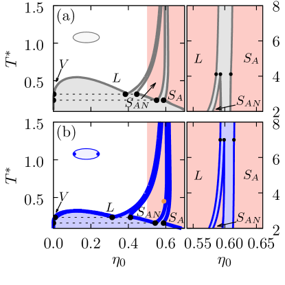
Figure 3: Panel (a) shows the phase diagram for ordinary liquid crystals with $L/R=2$ and $\varepsilon_{R}/\varepsilon_{L}=2$. Panel (b) corresponds to ionic liquid crystals described by $L/R=2,\varepsilon_{R}/\varepsilon_{L}=2,D/R=0.9,\lambda_{D}/R=5$, and $\gamma/(R\varepsilon_{0})=0.0045$. The black dots connected by a dashed line in the left panels indicate three-phase coexistence of the vapor ($V$), the liquid ($L$), and the narrow smectic $S_{AN}$ phase, and three-phase coexistence of the vapor, the $S_{AN}$, and the ordinary smectic $S_{A}$ phase, respectively. The black dots in the right panels indicate the location of $L$-$S_{AN}$-$S_{A}$ three-phase coexistence (here the connection by dashed lines is omitted) which occurs at the triple point temperature $T_{t}^{*}\approx 4.11$ for the ordinary liquid crystals and at $T_{t}^{*}\approx 7.0$ for the ILC fluid. The orange dot (${\color[rgb]{0.93359375,0.60546875,0.28515625}\bullet}$) denotes the state point $(T^{*}=0.45,\mu^{*}=20)$ in the ILC phase diagram for which, cf., Fig. 9 provides the corresponding order parameter profiles. The salmon-colored area represents the region $\eta_{0}\geq 0.5$ of the phase diagram for which the lateral spacing in between neighboring particles on a hexagonal lattice becomes less than $10\%$ of the particle diameter $R$, i.e., $a/R\leq 1.1$. Thus, the particles are densely packed and previous simulations suggest the occurrence of crystallization in this high density regime de Miguel and Vega (2002). According to the left panels the left bottom corner of the $S_{AN}$ phase appears to be stable against crystallization.

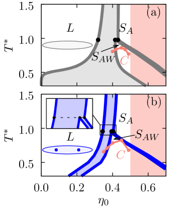
Figure 4: Panel (a) shows the phase diagram for ordinary liquid crystals with $L/R=4,\varepsilon_{R}/\varepsilon_{L}=2$ and panel (b) for ionic liquid crystals described by $L/R=4,\varepsilon_{R}/\varepsilon_{L}=2,D/R=0.9,\lambda_{D}/R=5$, and $\gamma/(R\varepsilon_{0})=0.045$. The black dots indicate the location of $L$-$S_{AW}$-$S_{A}$ three-phase coexistence and the inset in panel (b) gives an enlarged view of the vicinity of the triple point of the ILC fluid. The pink curve indicates the onset of crystallization ($C$), obtained by the method described in Sec. II.2.3. We note, that this approach does not allow one to analyze two-phase regions involving the phase $C$, because it compares the grand potential minima associated with smectic-A and crystalline phases for given $(\eta_{0},T^{*})$. Like in Fig. 3, the salmon-colored area represents the region $\eta_{0}\geq 0.5$ of the phase diagram for which the lateral spacing in between neighboring particles on a hexagonal lattice becomes less than $10\%$ of the particle diameter $R$, i.e., $a/R\leq 1.1$. Hence, the particles are densely packed and previous simulations report the occurrence of a solid phase in this density regime de Miguel and Vega (2002).

The phase behavior of ILCs and ordinary liquid crystals is studied by considering their respective phase diagrams in the $(T^{*},\eta_{0})$ plane. In Fig. 3(a) uncharged liquid crystals of length-to-breadth ratio $L/R=2$ and with Gay-Berne anisotropy parameter $\varepsilon_{R}/\varepsilon_{L}=2$ are considered. In Fig. 3(b) the phase behavior of ionic liquid crystals is shown, described by $L/R=2,\varepsilon_{R}/\varepsilon_{L}=2,D/R=0.9,\lambda_{D}/R=5,$ and $\gamma/(R\varepsilon_{0})=0.0045$. In both cases, at low packing fractions and at low temperatures, we observe the coexistence of a dilute and a dense isotropic phase, which we refer to as liquid ($L$)-vapor ($V$) coexistence. One finds that the critical temperature is lowered for the ILC fluid, which is a well-known observation for ionic systems Fisher (1994); here it is induced by the enhanced repulsion between the ILC molecules. Although low critical temperatures are a general feature of Coulombic systems, the precise location of the critical point is very sensitive to the details of the model and the method used Fisher (1994). For both types of fluids, increasing the mean packing fraction $\eta_{0}$ leads to a first-order phase transition to a smectic phase, in agreement with the corresponding results in Ref. Kondrat et al. (2010). Remarkably, at sufficiently low temperatures, before forming an ordinary smectic-A structure ($S_{A}$), a smectic phase appears in which the particles are oriented predominantly perpendicular to the director of the smectic phase, i.e., the $z$-direction along which the periodically oscillating density occurs. Since this behavior leads to a layer spacing which is comparable to the diameter $R$ of the particles and therefore is narrower (N) than in an ordinary $S_{A}$ phase, in which the layer spacing is comparable to the length $L$ of the particles, we refer to this smectic structure as the $S_{AN}$ phase. (Figure 7 provides a comparison of the structure of both types of smectic phases, $S_{AN}$ and $S_{A}$, for particles with length-to-breadth ratio $L/R=2$.) However, at high temperatures a first-order phase transition occurs directly from the liquid ($L$) to the $S_{A}$ phase. The low- and the high-temperature regimes are separated by a triple point, indicated by the black dots in the respective plot of Fig. 3, at which the liquid ($L$), the narrow smectic ($S_{AN}$), and the ordinary smectic phase ($S_{A}$) coexist. For the ionic liquid crystal the triple point temperature ($T_{t}^{*}\approx 7.0$) is significantly higher than for the ordinary uncharged liquid crystal ($T_{t}^{*}\approx 4.11$). Thus for ILCs the orientationally less-ordered smectic phase $S_{AN}$ remains stable at temperatures which are higher than for the ordinary liquid crystals. For large $T^{*}$ the $L$-$S_{A}$ coexistence curves coincide for liquid crystals and ILCs, because in the high-temperature regime the same hard-core repulsion is the dominant interaction.

In the context of (uncharged) ordinary liquid crystals, to our knowledge the $S_{AN}$ phase has not been reported previously. Since particles with length-to-breadth ratio $L/R=2$ and Gay-Berne anisotropy parameter $\varepsilon_{R}/\varepsilon_{L}=2$ exhibit a rather isotropic pair potential $U(\boldsymbol{r}_{12},\boldsymbol{\omega}_{1},\boldsymbol{\omega}_{2})$, it is very likely that the occurrence of liquid-crystalline phases in such a system is an artifact of the DFT method described in Sec. II.2.1, which is unable to capture the formation of genuine crystalline structures. For a hexagonal lattice structure the lateral lattice spacing $\frac{a}{R}=\sqrt{\frac{\pi}{3\sqrt{3}\eta_{0}}}$ (see Sec. II.2.3) takes a value of $a/R\approx 1.1$ for $\eta_{0}\approx 0.5$. Since this means that the free space $(a-R)/R$ in lateral direction in between neighboring particles on the hexagonal lattice is less than 10% of their diameter $R$, the particles are densely packed in the high density region $\eta_{0}\geq 0.5$ and previous simulations de Miguel and Vega (2002) on systems of pure (i.e., uncharged) Gay-Berne particles of length-to-breadth ratio $L/R=3$ report the occurrence of a solid phase for number densities $n_{0}\gtrsim 0.32\,R^{-3}$ (denoted as $\varrho$ in Ref. de Miguel and Vega (2002)) which correspond to $\eta_{0}=n_{0}LR^{2}\pi/6\gtrsim 0.5$ for $L/R=3$. Thus, as is shown by the salmon-colored area in Fig. 3 the thermodynamically stable state points of the liquid crystalline phases $S_{A}$ and $S_{AN}$ lie almost completely inside this (expected) crystallization region. We note, that the occurrence of two different types of “smectic” phases (i.e., $S_{A}$ and $S_{AN}$) within the DFT approach of Sec. II.2.1 can be a hint on the presence of actually different types of crystalline phases in such systems, which are distinguishable either by their lattice structure or by the degree of orientational ordering of the particles on the lattice sites. Within this interpretation of the phase diagrams in Fig. 3 the $S_{A}$ phase would be the analogue of a crystalline phase with additional orientational ordering, while the $S_{AN}$ phase mimics a crystalline phase with a lower degree of orientational ordering (i.e., a plastic crystal)

Figure 4 provides another comparison between (a) uncharged liquid crystal molecules and (b) ILC molecules with $D/R=0.9,\lambda_{D}/R=5,\gamma/(R\varepsilon_{0})=0.045$; both types of molecules share the same length-to-breadth ratio $L/R=4$ and the ratio $\varepsilon_{R}/\varepsilon_{L}=2$. These particles are twice as elongated as those in Fig. 3. In this case there is no $L$-$V$ coexistence; however, for the uncharged liquid crystal (a) it is still metastable, giving rise to a shoulder-like shape of the left hand side of the liquid-smectic two-phase region indicated by the gray-colored area in Fig. 4(a). For the ILC fluid the liquid-smectic two-phase region (light-blue-colored area in Fig. 4(b)) is narrower compared to its counterpart for the ordinary liquid crystals. At low temperatures this gives rise to stability of smectic structures, with respect to the isotropic liquid phase, already at smaller mean packing fractions $\eta_{0}$. This is caused by the presence of the additional electrostatic repulsion which imposes an energetic penalty on a homogeneous liquid already at packing fractions which are smaller than the corresponding ones for ordinary liquid crystal fluids. Similar to the previous case of the shorter particles, two distinct types of smectic structures can be observed. At sufficiently low temperatures, before forming an ordinary smectic-A structure ($S_{A}$) upon increasing $\eta_{0}$, a smectic phase is observed the layer spacing of which is considerably larger than in the high-temperature $S_{A}$ phase. Remarkably, it shows an alternating structure in which a majority of the particles within the smectic layers is oriented predominantly parallel to the director and a minority of the particles is located in between the layers with an orientation which is predominantly perpendicular to the director. Since to our knowledge such a bulk structure has not yet been observed in the context of smectic phases, we shall refer to this novel structure as the $S_{AW}$ phase, emphasizing the extraordinarily wide (W) layer spacing. Again three-phase coexistence occurs as indicated by black dots in the respective plots. It marks the transition to the high-temperature regime in which a first-order phase transition directly from the liquid to the $S_{A}$ phase takes place. In both cases (Figs. 4(a) and (b)) the triple point temperature is about $T_{t}^{*}\approx 1.0$. We note that the $S_{AW}$ phase has not been observed for ordinary liquid crystals, because commonly at low temperatures Gay-Berne fluids exhibit crystalline phases, as shown by previous studies de Miguel et al. (2004). In order to estimate the onset of crystallization in these systems, we have calculated the corresponding coexistence curves, shown as pink curves in Fig. 4, for a smectic-A phase $S_{A}$ and a hexagonal lattice structure $C$, by using the method of Sec. II.2.3. It turns out that the onset of crystallization appears close to the $S_{A}$-$S_{AW}$ transition for both cases in Fig. 4. This result suggests that at most in a small thermodynamic pocket the $S_{AW}$ phase remains stable against crystallization. Considering the simplicity of the method used (see Sec. II.2.3), which does not allow one to precisely determine the onset of crystallization, the stability of the $S_{AW}$ for those two cases (a) and (b) seems to be an artifact of the approximations used. Thus, one cannot expect a genuine $S_{AW}$ phase to occur for the two cases considered in Fig. 4, which is in agreement with previous findings. Nevertheless the $S_{AW}$ phase can be stable for an ILC fluid, because the presence of the charges is capable to alter the bulk phase diagram significantly. In the next section we shall discuss the influence of the location of the charges on the phase diagram and we shall demonstrate that one can enhance the stability of the $S_{AW}$ phase at higher temperatures by positioning the charges at the tips of the particles. Finally, Monte Carlo simulations for such kind of ILC fluids will be presented. The simulation results show that the $S_{AW}$ phase is indeed observable for ionic liquid crystal fluids. Finally we note that in order to study the onset of crystallization quantitatively on a more precise level, one should consider a free energy functional which accounts for positional correlations more carefully than the present DFT approach (see Sec. II.2). Treating the hardcore interactions of the anisotropic particles within fundamental measure theory Rosenfeld (1994); Hansen-Goos and Mecke (2009, 2010); Wittmann et al. (2015, 2016) is an appropriate and promising approach.

III.1.2 Dependence on the location of the charges

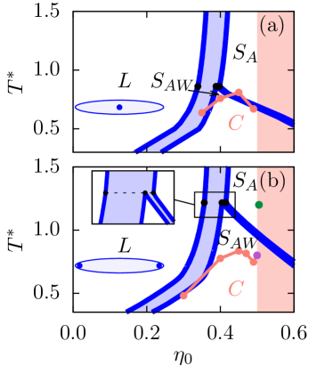
Figure 5: Phase diagrams for ILCs with (a) $L/R=4,\varepsilon_{R}/\varepsilon_{L}=2,D/R=0,\lambda_{D}/R=5$, and $\gamma/(R\varepsilon_{0})=0.045$ and (b) $L/R=4,\varepsilon_{R}/\varepsilon_{L}=2,D/R=1.8,\lambda_{D}/R=5$, and $\gamma/(R\varepsilon_{0})=0.045$. The colored dots denote the state points $(T^{*},\mu^{*})=(0.8,20)$ (${\color[rgb]{0.73046875,0.33203125,0.828125}\bullet}$, see, cf., Fig. 11) and $(1.2,18)$ (${\color[rgb]{0,0.546875,0.26953125}\bullet}$, see, cf., Fig. 10), while the black dots indicate $L$-$S_{AW}$-$S_{A}$ three-phase coexistence. The inset in panel (b) gives an enlarged view of the vicinity of the triple point. Like in Fig. 4, the pink curve indicates the onset of crystallization and the salmon-colored area represents the region $\eta_{0}\geq 0.5$ of the phase diagram for which the lateral spacing in between neighboring particles on a hexagonal lattice becomes less than $10\%$ of the particle diameter $R$, i.e., $a/R\leq 1.1$. Hence, the particles are densely packed and previous simulations report the occurrence of a solid phase in this density regime de Miguel and Vega (2002).

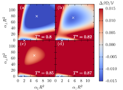
Figure 6: Grand potential density $\Delta\beta\Omega/\mathcal{V}$ (Eq. (34)) of spatially non-uniform structures (crystalline or smectic, Eq. (31)) in the range $\alpha_{\perp}R^{2}\in[0,120]$ and $\alpha_{||}R^{2}\in[0,12]$ relative to that for a spatially uniform nematic fluid of the same density at packing fraction $\eta_{N}=0.42$ and temperatures $T^{*}=0.8,0.82,0.85,$ and $0.87$. Crosses ($\times$) denote local minima of $\Delta\beta\Omega/\mathcal{V}$. By construction one has $\Delta\beta\Omega/\mathcal{V}=0$ for $\alpha_{||}=\alpha_{\perp}=0$. For $T^{*}=0.8$ (panel (a)) the global minimum of $\Delta\beta\Omega/\mathcal{V}$ is at $(\alpha_{||}R^{2}\approx 6,\alpha_{\perp}R^{2}\approx 80)$ which is a hexagonal crystal structure. The $S_{A}$ phase with $(\alpha_{||}R^{2}\approx 2,\alpha_{\perp}R^{2}=0)$ is metastable. By increasing temperature one finds coexistence of the $S_{A}$ phase and of the crystal to occur close to $T^{*}=0.82$ (panel (b)) and for larger temperature $T^{*}=0.85,0.87$ (panels (c) and (d)) the $S_{A}$ phase becomes stable.

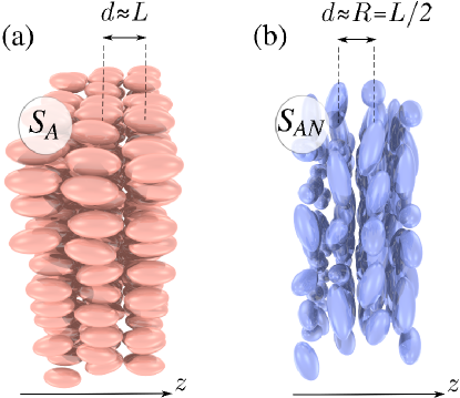
Figure 7: Smectic configurations of particles with $L/R=2$. Panel (a) depicts three layers of an ordinary smectic $S_{A}$ phase for a system composed of particles of length-to-breadth ratio $L/R=2$. The particles are mostly aligned with the layer normal (i.e., the $z$-direction), which leads to a layer spacing comparable to the size of the particle length $L$, as expected for an ordinary $S_{A}$ phase. Panel (b) represents a typical configuration of the $S_{AN}$ phase for $L/R=2$. Four smectic layers are shown in which the particles are oriented mainly perpendicular to the layer normal (i.e., the $z$-direction). However, they do not show a preferred orientation in the $x$-$y$-plane. This behavior leads to a layer spacing $d$ which is comparable to the size of the particle diameter $R$. In order to clearly visualize the smectic layers of the $S_{AN}$ phase, the diameter of the blue particles in panel (b) is reduced slightly. This leads to a small gap in between the smectic layers of this illustration. We note, that the smectic-A phases shown in panel (a) and (b) could not be observed in simulations and thus the depicted configurations are not snapshots but have been composed artificially for illustration purposes.

Here we investigate the dependence of the phase behavior of ILCs on the position $D$ of the charges of the particles for $L/R=4$, $\varepsilon_{R}/\varepsilon_{L}=2$, $\lambda_{D}/R=5$, $\gamma/(R\varepsilon_{0})=0.045$. Figure 5(a) shows the case of the two charges merged in the geometrical center of the molecule, i.e., $D/R=0$. In Fig. 5(b) the two charges are located near the tips, i.e., $D/R=1.8$. For $D/R=0$ the phase diagram coincides almost quantitatively with the corresponding phase diagram in Fig. 4(b) for $D/R=0.9$, besides a slight change in the location of the $S_{AW}$-$S_{A}$ two-phase region. Thus, the change in the pair potential by moving the charges from the center to the moderate distance $D/R=0.9$ turns out to be insufficient for a significant change of the phase behavior. However, moving the charges to the tips of the particles changes the shape of the pair potential significantly (Figs. 2(c) and (d)), and this leads indeed to a considerable change in the phase behavior. Figure 5(b) shows that for ILC molecules with charges at their tips ($D/R=1.8$ and $L/R=4$) the $L$-$S_{AW}$-$S_{A}$ triple point (see the inset of Fig. 5(b) providing an enlarged view of the vicinity of the triple point) is shifted to a higher temperature $T_{t}^{*}\approx 1.22$. Thus the low-temperature smectic phase $S_{AW}$ becomes stable at temperatures, which are higher than in the cases in Figs. 4 and 5(a). Again, we estimate the location of the onset of crystallization by employing the method of Sec. II.2.3. The corresponding results (pink curves in Fig. 5) show that, in the case of the charges being located right at the tips (panel (b)) the stable region of the $S_{AW}$ phase is enhanced compared with the other cases (Figs. 4 and 5(a)), due to the higher $L$-$S_{AW}$-$S_{A}$ triple point temperature. Hence, an $S_{AW}$ phase is expected to indeed occur for long thin particles with charges located at the tips (Fig. 5(b)), whereas it is preempted by crystallization otherwise (Figs. 4 and 5(a)). If the charges are localized at the tips of the molecules, the smectic phase $S_{AW}$ with wide layer spacing is stabilized in the intermediate temperature regime, i.e., in between the high temperature ordinary smectic $S_{A}$ phase and crystalline structures $C$ at low temperatures (at intermediate densities), which is due to the effective electrostatic repulsion of neighboring smectic layers. However, in the other cases, i.e., if the charges are localized close to the center of mass or if there are no charges at all, the ordinary smectic phase $S_{A}$ with densely packed smectic layers ($d\approx L$) is entropically preferred over the wide smectic phase $S_{AW}$ at intermediate temperatures (and intermediate packing fractions). However, in the present case, the $S_{AW}$ phase is more stable than the ordinary smectic $S_{A}$ phase only at temperatures below the freezing transition where the actually stable phase is the crystalline one.

We have studied the latter case of ILCs with the charges at their tips also by using grand canonical Monte Carlo simulations. In Fig. 8 two configurations are shown which appear during simulations performed for $(T^{*},\mu^{*})=(0.6,0.9)$ in panel (a), and for $(T^{*},\mu^{*})=(0.5,-2.6)$ in panel (b). Here the pair potential is described by $L/R=4$, $\varepsilon_{R}/\varepsilon_{L}=3$, $D/R=1.8$, $\lambda_{D}/R=5$, $\gamma/(R\varepsilon_{0})=0.045$, and $R_{\text{cut}}/R=6$. The chemical potentials are chosen to be sufficiently large, such that in both cases the system forms a smectic structure. In panel (a), one observes an ordinary $S_{A}$ phase according to which the particles are located in the smectic layers with a preferred orientation parallel to the director $\boldsymbol{\hat{n}}$, i.e., the layer normal. Instead, at the lower temperature $T^{*}=0.5$ panel (b) shows a different structure. Here, an increased layer spacing is observed. The space in between the layers is populated by numerous particles which are preferentially oriented perpendicular to the layer normal. This is the same periodic structure which we have found within our DFT approach for the low-temperature $S_{AW}$ phase (compare Fig. 5(b)). Furthermore, in agreement with the present theory, increasing the rescaled chemical potential $\mu^{*}$ at low but fixed temperature $T^{*}$, at sufficiently large packing fraction $\eta_{0}$ one finds a transition from the $S_{AW}$ phase to the $S_{A}$ phase. By increasing the chemical potential $\mu^{*}$ the packing fraction is also increased and ultimately a dense packing of smectic layers, corresponding to the $S_{A}$ phase, is preferred over the smectic $S_{AW}$ phase with wide layer spacing. (See also the discussion of our simulational results in the next section.)

It is worth mentioning that a similar kind of structure has been reported for a system of hard discs interacting via an additional anisotropic Yukawa potential Jabbari-Farouji et al. (2013, 2014). In this canonical Monte Carlo study a structure called intergrowth texture has been observed which shows a periodic structure of two alternating layers of particles. The directors of both layers are perpendicular to each other. Nevertheless, unlike the $S_{AW}$ phase, the particles within each layer of an intergrowth texture are not localized. Thus they do not exhibit positional order in any direction and cannot be categorized as a smectic structure. In contrast to monodisperse systems, like in the present study, alternating smectic layer structures have already been observed in binary mixtures of particles with different geometries Koda and Kimura (1994); van Roij and Mulder (1996); Cinacchi et al. (2004); Martínez-Ratón et al. (2005). For such systems the alternating layer structure is driven by segregation of the two particles species. It is worth mentioning, that due to fluctuations, even in the common $S_{A}$ phase there is a non-vanishing probability to find particles in between the smectic layers with perpendicular orientation (see, e.g., Ref. van Roij et al. (1995)).

Finally, we note that for instance particles with a electric quadrupole are known to form smectic $S_{C}$ phases, in which the director $\boldsymbol{\hat{n}}$ is tilted with respect to the normal of the smectic layers (see, e.g., Ref. Neal and Parker (1998)). Such kind of liquid crystals are of particular interest for technological applications such as fast electro-optic displays, because those materials can be ferroelectric Meyer et al. (1975).

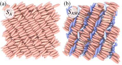
Figure 8: Smectic configurations of ILCs with $L/R=4$. Panel (a) shows a configuration appearing during a simulation performed at temperature $T^{*}=0.6$; the chemical potential $\mu^{*}=0.9$ is tuned such that $\eta_{0}\approx 0.389$. Panel (b) depicts a configuration for $(T^{*},\mu^{*})=(0.5,-2.6)$ giving rise to $\eta_{0}\approx 0.324$. For both (a) and (b) the parameters of the pair potential are given by $L/R=4,\varepsilon_{R}/\varepsilon_{L}=3,D/R=1.8,\lambda_{D}/R=5,\gamma/(R\varepsilon_{0})=0.045$, and $R_{\text{cut}}/R=6$. At the higher temperature $T^{*}=0.6$, one finds the ordinary smectic $S_{A}$ phase, while for the lower temperature $T^{*}=0.5$ the novel $S_{AW}$ phase is observed. The latter is characterized by an alternating structure of particles such that within the smectic layers the particles are oriented parallel to the layer normal (pale pink particles) whereas the particles in between the layers are oriented perpendicularly to it but without lateral orientational order (blue particles).

III.2 Variety of smectic structures

We have illustrated how the phase behavior of ionic liquid crystals varies as function of the parameters characterizing the pair potential. In particular, the occurring smectic phases show distinct layer spacings. In order to analyze the structure of the various smectic bulk phases in more detail, we discuss the density profiles in terms of the local packing fraction $\eta(z)=n(z)\,LR^{2}\pi/6$ and the spatially varying orientational order parameter $S_{2}(z)$ (compare Sec. II.2.1).

Figure 9: Local packing fraction $\eta(z/R)=n(z/R)LR^{2}\pi/6$ and orientational order parameter $S_{2}(z/R)=\int_{\mathcal{S}}\!\mathrm{d}^{2}{\omega}\;P_{2}(\cos(\vartheta))\varrho(z/R,\vartheta)/n(z/R)$ with the total number density $n(z/R)=\int_{\mathcal{S}}\!\mathrm{d}^{2}{\omega}\;\varrho(z/R,\vartheta)$ displayed within one period $d/R\approx 1.2$ for the state point $(T^{*},\mu^{*})=(0.45,20)$ indicated in Fig. 3(a) (orange dot ${\color[rgb]{0.93359375,0.60546875,0.28515625}\bullet}$) for $L/R=2,\varepsilon_{R}/\varepsilon_{L}=2,D/R=0.9,\lambda_{D}/R=5$, and $\gamma/(R\varepsilon_{0})=0.0045$. The smectic layer spacing $d$ is smaller than the length of the particles. At the center of the smectic layers the ILC molecules are oriented mainly perpendicular to the layer normal $\boldsymbol{\hat{n}}$ as one can infer from the negative value of the orientational order parameter $S_{2}(z=0)\approx-0.4$ ($S_{AN}$ phase).

First, we consider the smectic phase $S_{AN}$ observed for $L/R=2,\varepsilon_{R}/\varepsilon_{L}=2,D/R=0.9,\lambda_{D}/R=5$ and, $\gamma/(R\varepsilon_{0})=0.0045$ (compare Fig. 3(b)). In Fig. 9 the relevant profiles $\eta(z)$ and $S_{2}(z)$ are plotted for the state point $(T^{*},\mu^{*})=(0.45,20.0)$ indicated in Fig. 3(b) (orange dot ${\color[rgb]{0.93359375,0.60546875,0.28515625}\bullet}$). The smectic layer spacing is $d/R\approx 1.2$; $S_{2}(z)\approx-0.4$ at $|z/d|\ll 1$ shows that within the smectic layers the particles are oriented predominantly perpendicular to the layer normal. This finding is plausible because $d/R\approx 1.2$ is much smaller than the length of the particles $L/R=2$ which enforces the particles to tilt towards the smectic layers. The packing fraction profile $\eta(z)$ in Fig. 9 tells that the particles are strongly localized within the layers. The layer spacing does not vary significantly as function of temperature and of the chemical potential within the thermodynamic region of a stable smectic phase (according to the DFT method introduced in Sec. II.2.1). In the smectic $S_{AN}$ phase the layer normal $\boldsymbol{\hat{n}}$ still points into the $z$-direction, so that the particles do not have a preferred lateral orientation, but they avoid an orientation parallel to the director. This behavior seems to be caused by the small length-to-breadth ratio $L/R=2$ and the small value of the anisotropy parameter $\varepsilon_{R}/\varepsilon_{L}=2$, which renders these particles relatively isotropic. This is even more pronounced in the case of the ILC fluid shown in Fig. 3(b) due to the additional electrostatic repulsion, which leads to a higher $L$-$S_{AW}$-$S_{A}$ triple point temperature. For both smectic phases, $S_{A}$ and $S_{AN}$, the layer spacing does not vary significantly as function of temperature and chemical potential within the thermodynamic region of a stable smectic phase. Again, we emphasize that for the shorter particles, described by $L/R=2$ and $\varepsilon_{R}/\varepsilon_{L}=2$, the stability of the liquid-crystalline phases $S_{A}$ and $S_{AN}$ is very likely to be an artifact of the method employed (see Sec. II.2.1). The transition from an isotropic liquid phase to those mesophases occurs at large densities for which one already expects crystalline structures to emerge (see the discussion in Sec. III.1.1).

Figure 10: Local packing fraction $\eta(z/R)$ and scalar orientational order parameter $S_{2}(z/R)$ within one period $d/R\approx 4.5$ at the state point $(T^{*},\mu^{*})=(1.2,18)$ in Fig. 5(b) (green dot ${\color[rgb]{0,0.546875,0.26953125}\bullet}$) for $L/R=4,\varepsilon_{R}/\varepsilon_{L}=2,D/R=1.8,\lambda_{D}/R=5$, and $\gamma/(R\varepsilon_{0})=0.045$. The ILC molecules are strongly localized in the center of the smectic layers where they are oriented mainly parallel to the layer normal $\boldsymbol{\hat{n}}$ as indicated by the large positive value of the orientational order parameter $S_{2}(z=0)\approx 0.9$ (ordinary $S_{A}$ phase).

Figure 11: Local packing fraction $\eta(z/R)$ and scalar orientational order parameter $S_{2}(z/R)$ within one period $d/R\approx 7.7$ at the state point $(T^{*},\mu^{*})=(0.8,20)$ in Fig. 5(b) (magenta dot ${\color[rgb]{0.73046875,0.33203125,0.828125}\bullet}$) for $L/R=4,\varepsilon_{R}/\varepsilon_{L}=2,D/R=1.8,\lambda_{D}/R=5$, and $\gamma/(R\varepsilon_{0})=0.045$. One observes an alternating structure with the majority of the particles being located at the center of the layers ($z\approx 0$) with an orientation parallel to the layer normal, while a significant minority of particles is located in between the layers (i.e., $|z|/R\approx d/(2R)\approx 3.85$) with preferentially perpendicular orientation ($S_{AW}$ phase).

Now, we turn to the ILC molecules described by the parameter set $L/R=4,\varepsilon_{R}/\varepsilon_{L}=2,D/R=1.8,\lambda_{D}/R=5$, and $\gamma/(R\varepsilon_{0})=0.045$, the phase diagram of which is shown in Fig. 5(b). In Fig. 5(b), at the state point $(T^{*},\mu^{*})=(1.2,18)$ (green dot ${\color[rgb]{0,0.546875,0.26953125}\bullet}$) the $S_{A}$ phase is stable with a layer spacing $d/R\approx 4.5$. The profiles of $\eta(z)$ and $S_{2}(z)$ are shown in Fig. 10. As expected for an ordinary smectic-A phase, the ILC molecules are located in the layers with an orientation predominantly parallel to the layer normal $\boldsymbol{\hat{n}}$. In contrast to the shorter particles discussed in Fig. 9, here the layer spacing $d/R\approx 4.5$ is comparable with the size of the length $L/R=4$ of the particles and thus there is enough space for the particles to be aligned with the layer normal $\boldsymbol{\hat{n}}$.

At low temperatures and large packing fractions, one finds the novel wide smectic $S_{AW}$ phase. For $(T^{*},\mu^{*})=(0.8,20)$ (magenta dot ${\color[rgb]{0.73046875,0.33203125,0.828125}\bullet}$ in Fig. 5(b)) this structure is shown in Fig. 11. The equilibrium layer spacing is $d/R\approx 7.7$, which is significantly larger than the one for the high-temperature ordinary smectic $S_{A}$ phase (compare Fig. 10). The wide smectic $S_{AW}$ phase shows an increased number of particles localized in between the layers, i.e., around $|z|\approx d/2$. They are oriented preferentially perpendicular to the layer normal $\boldsymbol{\hat{n}}$ (with no orientational ordering within the $x$-$y$-plane), while particles in the layers, i.e., for $|z/d|\ll 1$, are predominantly aligned with the normal $\boldsymbol{\hat{n}}$, like in the $S_{A}$ phase.

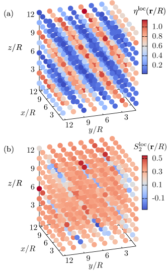
Figure 12: Local packing fraction $\eta^{\text{loc}}(\boldsymbol{r}/R)$ (a) and scalar orientational order parameter $S_{2}^{\text{loc}}(\boldsymbol{r}/R)$ (b) obtained from grand canonical Monte Carlo simulations on a periodic cubic box of side length $V^{1/3}/R=13.2$ at temperature $T^{*}=0.5$ and chemical potential $\mu^{*}=-1.2$, giving rise to a global mean packing fraction $\eta_{0}\approx 0.436$ in the simulation box. Each colored dot represents a site of a simple cubic lattice on which we monitor $\eta^{\text{loc}}(\boldsymbol{r}/R)$ and $S_{2}^{\text{loc}}(\boldsymbol{r}/R)$, respectively, along the MC trajectory. The color-coding of the dots can be inferred from the respective color key. The parameters of the pair potential are given by $L/R=4,\varepsilon_{R}/\varepsilon_{L}=3,D/R=1.8,\lambda_{D}/R=5,\gamma/(R\varepsilon_{0})=0.045$, and $R_{\text{cut}}/R=6$. The ILC molecules are concentrated in the smectic layers which are oriented mainly parallel to the layer normal, which can be inferred from the positive value of $S_{2}^{\text{loc}}(\boldsymbol{r}/R)>0.3$ for positions $\boldsymbol{r}$ which correspond to large $\eta^{\text{loc}}(\boldsymbol{r}/R)>0.6$; this corresponds to an ordinary smectic $S_{A}$ phase. Some sample points $\boldsymbol{r}$ yield a negative value of $S_{2}(\boldsymbol{r}/R)<0$, corresponding to particles which eventually moved out of the smectic layers and then turned perpendicular. Here, in contrast to the DFT approach, the layer normal does not necessarily point into the $z$-direction, but it is tilted towards one of the edges of the simulation box.

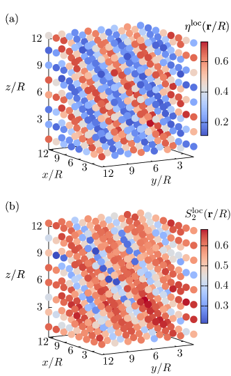
Figure 13: Same as Fig. 12 but for $T^{*}=0.6$ and $\mu^{*}=1.7$ which corresponds to $\eta_{0}\approx 0.394$. This state point belongs to an ordinary smectic $S_{A}$ phase, which can be inferred from the positive value of $S_{2}^{\text{loc}}(\boldsymbol{r}/R)>0.4$ for positions $\boldsymbol{r}$ which correspond to large $\eta^{\text{loc}}(\boldsymbol{r}/R)>0.6$. The temperature $T^{*}=0.6$ is higher than for the state point $(0.5,-1.2)$ discussed in Fig. 12. Thus the particles in the smectic layers are less localized leading to smaller maximum values of the local packing fraction $\eta_{\text{max}}^{\text{loc}}(\boldsymbol{r}/R)\approx 0.7$ (compare the maxima $\eta_{\text{max}}^{\text{loc}}(\boldsymbol{r}/R)\approx 1.1$ in Fig. 12). The layer normal points towards one of the diagonals of the simulation box.

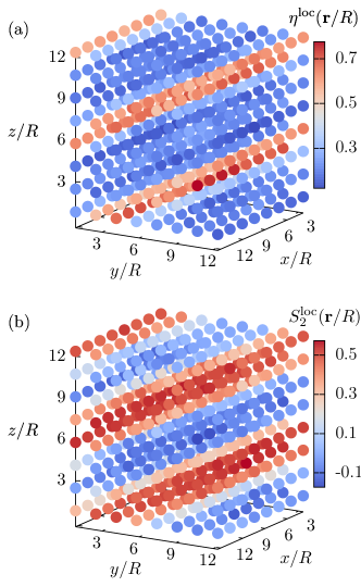
Figure 14: Same as Figs. 12 and 13 but for $T^{*}=0.5$ and $\mu^{*}=-2.6$ which corresponds to $\eta_{0}\approx 0.324$. For this state point one observes an alternating structure of a majority of particles, which are located in the layers with their orientations parallel to the layer normal, while a significant minority of the particles is located in between the layers with perpendicular orientation ($S_{AW}$ phase). The layer normal points towards one of the edges of the simulation box.

So far, we have discussed the structural properties of the various ILC smectic phases, as predicted by the present density functional theory. For comparison, in Figs. 12, 13, and 14 the local packing fraction $\eta^{\text{loc}}(\boldsymbol{r})=\varrho^{\text{loc}}(\boldsymbol{r})\,LR^{2}\pi/6$ and the local orientational order parameter $S_{2}^{\text{loc}}$, as obtained by Monte Carlo simulations of an ILC fluid with $L/R=4,\varepsilon_{R}/\varepsilon_{L}=3,\lambda_{D}=5,D/R=1.8,\gamma/(R\varepsilon_{0})=0.045$, and $R_{\text{cut}}/R=6$, are shown on a simple cubic lattice of sample points within the cubic simulation box of side length $V^{1/3}/R=13.2$. Figures 12 and 13 clearly show an ordinary smectic $S_{A}$ phase, characterized by a periodic structure in which the particles are located inside the smectic layers, indicated by the red data points for large values of $\eta^{\text{loc}}(\boldsymbol{r})$ and a predominant alignment of particles along the layer normal, indicated by the large positive value of the local orientational order parameter $S_{2}^{\text{loc}}(\boldsymbol{r})\geq 0.5$ for nearly all sample points $\boldsymbol{r}$. The data points of Fig. 12 are obtained for $(T^{*},\mu^{*})=(0.5,-1.2)$, i.e., $\eta_{0}\approx 0.436$ and the data of Fig. 13 corresponds to $(T^{*},\mu^{*})=(0.6,1.7)$, i.e., $\eta_{0}\approx 0.394$. However, if the temperature is sufficiently low and the chemical potential is chosen such that the mean packing fraction is not too large, e.g., $(T^{*},\mu^{*})=(0.5,-2.6)$ so that $\eta_{0}\approx 0.324$, one observes the novel smectic structure $S_{AW}$ as shown in Fig. 14. The alternating orientation of particles gives rise to the alternating pattern of blue ($S_{2}^{\text{loc}}(\boldsymbol{r})<0$) and red ($S_{2}^{\text{loc}}(\boldsymbol{r})>0$) data points for the orientational order parameter along the layer normal (Fig. 14(b)). For these simulation results the layer normal and the $z$-direction are not parallel, because the start configuration is isotropic, which in principle allows the system to form any structure without bias. (Without cost of free energy the sample can be rotated so that the layer normal is parallel to the $z$ axis.) However, the layer normal tends to be parallel to one of the diagonals of the simulation box (compare Figs. 12-14), which is likely to be related to the cubic geometry of the simulation box and thus appears to be a finite-size effect. In agreement with the present DFT approach, the simulations tell that for the $S_{A}$ phase the smectic layer spacing is of the size of the particle length $L/R=4$ while for the $S_{AW}$ phase $d$ is significantly larger. In this phase there are small (local) maxima of the local packing fraction $\eta^{\text{loc}}(\boldsymbol{r})$ in between the layers (indicated in Fig. 14 by the light blue dots being surrounded by dark blue dots). Note that although some sample points in Fig. 12 show a negative value of the local orientational order parameter $S_{2}^{\text{loc}}(\boldsymbol{r})<0$ in between the smectic layers, this does not indicate a realization of the smectic $S_{AW}$ phase, but is due to the well-known observation, that in course of the simulation some particles move out of the smectic layers and then turn perpendicular, because there is only a narrow gap in between the smectic layers of an ordinary $S_{A}$ phase (see, e.g., Ref. van Roij et al. (1995)).

The present DFT predicts that the triple point temperature for an ILC fluid can be increased relative to the corresponding one for an ordinary liquid crystal, provided the location $D$ of the charges, their interaction strength $\gamma$, and the screening length $\lambda_{D}$ are chosen suitably (compare Figs. 4 and 5). Therefore the $S_{AW}$ phase can occur for ILCs (see Fig. 8(b)) if the $S_{AW}$-$S_{A}$ coexistence curve is shifted above the melting transition. In contrast, for ordinary liquid crystals (see Fig. 4(a)) the formation of the $S_{AW}$ phase is preempted by crystallization, which is in agreement with the findings of previous studies, e.g., Ref. de Miguel et al. (2004).

It is worth mentioning, that the so-called intergrowth texture structure observed in Refs. Jabbari-Farouji et al. (2013, 2014) can also be interpreted as an ionic liquid crystal phenomenon, because there hard discs have been considered which interact via an additional, anisotropic Yukawa potential.

III.3 Temperature dependence of the layer spacing

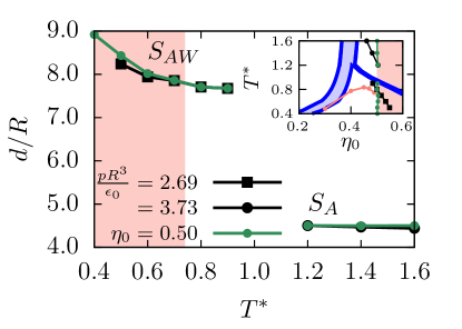
Figure 15: Equilibrium layer spacing $d/R$, as obtained within the present DFT approach, as function of temperature $T^{*}$ for the parameter set $L/R=4,\varepsilon_{R}/\varepsilon_{L}=2,D/R=1.8,\lambda_{D}/R=5$, and $\gamma/(R\varepsilon_{0})=0.045$ of the pair potential. For $T^{*}>1.0$ the ordinary smectic $S_{A}$ phase is stable (see the inset, which shows the considered thermodynamic paths). For the considered paths, the layer spacing depends only weakly on temperature. The pressure $p:=\Omega[\varrho^{\text{eq}}]/\mathcal{V}$ is obtained by multiplying Eq. (26) by $kT$. For the low-temperature wide smectic $S_{AW}$ phase the dependence on temperature is more pronounced. This is due to the free space in between the layers and the electrostatic repulsion, which becomes more effective upon decreasing temperature. However, this effect is prominent only in that region of the $S_{AW}$ phase where it is metastable with respect to crystallization, i.e., for $T^{*}\lesssim 0.74$ (salmon-colored area). The pink curve in the inset indicates the onset of crystallization.

The high-temperature phase $S_{A}$ and the low-temperature phase $S_{AW}$ exhibit distinct structural properties (Figs. 10 and 11). In particular the size of the layer spacing differs. Our analysis reveals that for the $S_{A}$ phase, in which the layer spacing is about the size of the length $L$ of the particles, the layer thickness varies only weakly as function of temperature (see Fig. 15). Along two thermodynamic paths within the domain of the stable $S_{A}$ phase – one at fixed mean packing fraction $\eta_{0}\approx 0.5$ (green dotted vertical path in the corresponding phase diagram shown in the inset of Fig. 15; compare Fig. 5(b)) and the other one at fixed pressure $p=-\Omega[\varrho^{\text{eq}}]/\mathcal{V}=3.73\,\varepsilon_{0}/R^{3}$ (black dotted path) – the layer spacing does not change much and takes a value of about $d/R\approx 4.4-4.5$, which is a common finding for phases of the $S_{A}$-tpe. Interestingly, for both paths (black squared path with $p=2.69\,\varepsilon_{0}/R^{3}$ and green dotted path with $\eta_{0}\approx 0.5$; $T^{*}\leq 0.9$) the low-temperature wide smectic phase $S_{AW}$, which, compared with the $S_{A}$ phase, exhibits an increased layer spacing (compare Figs. 10 and 11), also does not show a considerable temperature dependence of the layer spacing within its region of thermodynamic stability (see white background in Fig. 15 for $T^{*}\in[0.74,0.9]$). However, within the region of the $S_{AW}$ phase being metastable with respect to crystallization, i.e., for $T^{*}\lesssim 0.74$ in Fig. 15 (salmon-colored area), for both paths there is a pronounced temperature dependence of the layer spacing. Since the smectic layers of the $S_{AW}$ phase are not as densely packed as the layers of an ordinary $S_{A}$ phase, the free space in between the layers allows for a certain softness of the layer spacing. The increase of the layer spacing with decreasing temperature can be understood intuitively, because upon lowering temperature the electrostatic repulsion becomes more efficient so that the smectic layers widen. Nevertheless, since this behavior is only observable within the metastable region of the $S_{AW}$ phase, we conclude that one expects only a weak temperature dependence of the layer spacing for the $S_{AW}$ phase, analogous to the $S_{A}$ phase.

For the shorter particles with $L/R=2$, we have found both for the narrow $S_{AN}$ phase as well as for the ordinary $S_{A}$ phase a very weak dependence of the layer spacing on temperature, like in Fig. 15 for the high-temperature smectic $S_{A}$ phase.

IV Conclusions and Summary

Ionic liquid crystals have been investigated by means of density functional theory (Sec. II.2) and grand canonical Monte Carlo simulations (Sec. II.3). To this end a coarse-grained description of the ILC molecules (Fig. 1) as rigid ellipsoids interacting via a molecular pair potential $U(\boldsymbol{r}_{12},\boldsymbol{\omega}_{1},\boldsymbol{\omega}_{2})$ (Eq. (1) and Fig. 2) has been employed (see Sec. II.1).

This study demonstrates that ILC fluids show a rich phenomenology concerning their phase behavior and their structural bulk properties. Beyond the qualitative differences in the phase behavior of ordinary liquid crystals and ILCs, we have examined in detail the dependence of the thermal and structural properties of ILC fluids on the length-to-breadth ratio $L/R$ and on the distance $D$ of the charges from the geometrical center of the molecules. This analysis leads to the following main conclusions:

• Comparing ordinary (uncharged) liquid crystals and ILCs, within the present DFT approach a lowering of the liquid-vapor critical point of the latter is observed (see Fig. 3). Additionally, for ILCs the liquid-smectic two-phase region becomes narrower, giving rise to a stable smectic structure at smaller packing fractions $\eta_{0}$ (see Fig. 4).

• For the shorter particles with length-to-breadth ratio $L/R=2$ there is an ordinary $S_{A}$ phase at high temperatures and large mean packing fractions. At low temperatures and intermediate mean packing fractions there is a distinct smectic $S_{AN}$ structure in which the particles are oriented parallel to the smectic layers, i.e., perpendicular to the layer normal $\boldsymbol{\hat{n}}$ (see Fig. 9), and thus do not show a preferred orientation. (Figure 7 provides a comparison of the structure of both types of smectic phases, $S_{AN}$ and $S_{A}$, for particles with length-to-breadth ratio $L/R=2$.) This behavior seems to be related to the small length-to-breadth ratio $L/R=2$ and to the small value of the anisotropy parameter $\varepsilon_{R}/\varepsilon_{L}=2$ of the underlying Gay-Berne pair potential. This renders the particles rather isotropic, which is even more pronounced in the case of the ILC fluid (Fig. 3(b)) due to the additional electrostatic repulsion, and thus leads to a higher $L$-$S_{AN}$-$S_{A}$ triple point temperature. However, considering the large packing fractions $\eta_{0}\geq 0.5$ for which the liquid-crystalline phases are predicted to occur in these systems, we have found that for a hexagonal lattice structure this leads to a lateral lattice spacing of $a/R\leq 1.1$ (see Secs. II.2.3 and III.1.1). Hence, the particles are densely packed in this density regime and previous simulations de Miguel and Vega (2002) on systems of Gay-Berne particles of length-to-breadth ratio $L/R=3$ report the onset of crystallization within that regime. On this basis, at least in parts, the thermodynamic stability of the liquid-crystalline phases $S_{A}$ and $S_{AN}$ can be expected to be an artifact of the method employed (see Sec. II.2.1), which cannot capture crystalline phases. The prediction of the liquid-crystalline phases $S_{A}$ and $S_{AN}$, which show an periodically varying density profile in $z$-direction, can be considered as a hint on the presence of various types of crystalline phases at large densities in these systems. The $S_{A}$ phase can be interpreted as an analogue to a crystalline phase with additional orientational ordering, while the $S_{AN}$ phase mimics a crystalline phase with a lower degree of orientational ordering (i.e., plastic crystals).

• For the longer particles of length-to-breadth ratio $L/R=4$, besides the isotropic liquid ($L$) and the ordinary smectic $S_{A}$ phase (Fig. 10), at low temperatures and sufficiently large packing fractions the novel $S_{AW}$ phase (Fig. 11) occurs (see Figs. 4 and 5). It is characterized by a considerably larger layer spacing than in the ordinary $S_{A}$ phase (compare Figs. 10 and 11). While the majority of particles is oriented mostly parallel to the layer normal, as indicated by a large value of the orientational order parameter $S_{2}(z=0)>0.8$ within the smectic layers, a significant number of particles is located in between the smectic layers. Those particles tend to be perpendicular to the layer normal, giving rise to $S_{2}(|z|\lesssim d/2)<0$.

• Concerning the phase behavior of ILCs as function of the location of the charges in the molecules, we have found that for the parameter set $L/R=4,\lambda_{D}/R=5,\varepsilon_{R}/\varepsilon_{L}=2,\gamma/(R\varepsilon_{0})=0.045$ positioning the charges at an intermediate distance $D/R\leq 0.9$ from the geometric center does not alter the phase behavior much as compared to positioning the charges in the center (see Figs. 4(b) and 5(a)). However if the charges are located almost at the tips of the molecules ($L/R=4,D/R=1.8$, Fig. 5(b)) there is a significant change in the phase behavior. The coexistence of the phases $S_{AW}$ and $S_{A}$ is shifted towards higher temperatures. This shift for $D/R=1.8$ stabilizes the $S_{AW}$ phase in a temperature regime below the ordinary $S_{A}$ phase but above the melting curve, unlike the other cases studied (Figs. 4 and 5(b)) for which our analysis, using the method discussed in Sec. II.2.3, yields that the $S_{AW}$ phase is expected to be preempted by crystallization (compare the pink curves in Figs. 4 and 5 which are obtained by the procedure outlined in Fig. 6 ). Accordingly, we have observed the $S_{AW}$ phase, within our present grand canonical Monte Carlo simulations, for an ILC fluid the charges of which are located at the tips of the molecules. In qualitative agreement with DFT, the simulational results yield an ordinary smectic $S_{A}$ phase at high temperatures and large packing fractions (see Figs. 12 and 13); the layer spacing is of the size of the particles and nearly all of them are located within the smectic layers aligned with the layer normal (see Fig. 8(a)). At lower temperatures the novel $S_{AW}$ smectic phase with wide layer spacings occurs, such that a considerable fraction of particles is located in between the smectic layers with mainly perpendicular orientation with respect to the layer normal (see Figs. 8(b) and 14).

• Analyzing the dependence of the smectic layer spacing on temperature for the parameter set $L/R=4,\varepsilon_{R}/\varepsilon_{L}=2,\lambda_{D}=5,D/R=1.8,\gamma/(R\varepsilon_{0})=0.045$ reveals distinct behaviors of the smectic $S_{A}$ and $S_{AW}$ phases (see Fig. 15): While the layer spacing of the ordinary high-temperature smectic $S_{A}$ phase does not vary notably as function of temperature, which is a common finding for ordinary $S_{A}$ phases, increasing layer spacings for decreasing temperatures can be observed for the low-temperature smectic phase $S_{AW}$. This can be understood in terms of the free space in between the smectic layers which gives rise to a certain softness in the layer spacing. Due to the enhanced effective electrostatic repulsion at lower temperatures, the layers tend to widen upon lowering the temperature. However, this behavior is prominent only in the metastable region of the $S_{AW}$ phase, while within the stable region of the $S_{AW}$ phase, in analogy to the high-temperature $S_{A}$ phase, there is no pronounced temperature dependence of the layer spacing.

  Like the high-temperature $S_{A}$ phase for long particles (see Fig. 15), the layer spacing of the smectic $S_{A}$ and $S_{AN}$ phases, observed for shorter particles with $L/R=2$, does not exhibit a considerable temperature dependence.

We point out that the theoretical framework presented here is also applicable for studying interfaces such as the free interfaces of coexisting bulk phases or the interface of an ionic liquid crystal in contact with an electrode. In particular it will be interesting to study the interfacial features of these materials as they emerge from the interplay of ionic and liquid-crystalline properties. We also stress the importance of the choice of the projected density distribution $\bar{\varrho}(\boldsymbol{r},\boldsymbol{\omega})$ (Eq. 12) with respect to our theoretical approach, because the incorporation of second-order Fourier modes is indispensable for capturing the novel wide smectic $S_{AW}$ phase.

A natural extension of the study presented here is to consider a density functional of binary fluid mixtures allowing for an explicit description of the counterions. However, we do not expect the phase behavior to be crucially affected by this higher degree of sophistication, because studies using multicomponent integral equations Harnau and Reineker (2000); Harnau and Hansen (2002) showed that the counterions, which are smaller than the ILC molecules, give rise to an effective screening between the latter, rendering the use of a screened Coulomb potential, like in Eq. (5), a reasonable approach. However, a more realistic description could be obtained by determining the Debye screening length $\lambda_{D}$ in accordance with Eq. (6), instead of treating it as a control parameter with a fixed value $\lambda_{D}/R=5$. Within this approach, the full range of the Debye screening length in the various density and temperature regimes could be incorporated into the model, which could lead to interesting new phase behaviors and structural phenomena. While for dilute electrolyte solutions one typically finds $\lambda_{D}/R\gg 1$, in dense ionic liquids the Debye screening length $\lambda_{D}$ can become smaller than the particle diameter $R$. Thus, the value $\lambda_{D}/R=5$ used throughout this study lays in between those two limiting cases.

The description of the reference hard-core system within an approach more sophisticated than Eq. (30), such as fundamental measure theory, would allow for a more reliable calculation of the transition towards crystalline phases. We consider this as a necessary step in order to accurately predict the extent of $S_{AW}$ stability at low temperatures.

Induced by an external electric field, qualitatively new phenomena might occur.

Appendix A Derivation of Eq. (19)

As explained below Eq. (14), for bulk phases one has $Q_{i}=\text{const}$. Accordingly, Eq. (15) reduces to

$$\beta\psi_{\text{PL}}(\boldsymbol{r},\boldsymbol{\omega},[\bar{\varrho}])=-\mathcal{J}(Q_{0})\times$$

$$\int_{\mathcal{V}}\!\mathrm{d}^{3}{r^{\prime}}\;\int_{\mathcal{S}}\!\mathrm{d}^{2}{\omega^{\prime}}\;\bar{\varrho}(\boldsymbol{r}^{\prime},\boldsymbol{\omega}^{\prime})f_{M}(\boldsymbol{r}-\boldsymbol{r}^{\prime},\boldsymbol{\omega},\boldsymbol{\omega}^{\prime}).$$ (39)

Using the definition in Eq. (12) of the projected density $\bar{\varrho}(\boldsymbol{r},\boldsymbol{\omega})$, with $Q_{i}=\text{const}$ for bulk phases, we obtain six terms in the integrand of Eq. (39), one for each $Q_{i},~{}i=0,\cdots,5$. Changing the integration variable from $\boldsymbol{r}^{\prime}$ to $\boldsymbol{\tilde{r}}=\boldsymbol{r}^{\prime}-\boldsymbol{r}$ yields

$$\beta\psi_{\text{PL}}(\boldsymbol{r},\boldsymbol{\omega},[\bar{\varrho}]) =$$

$${\color[rgb]{0,0,0}-\frac{\mathcal{J}(Q_{0})}{4\pi}}\bigg{[}~{}Q_{0} \int_{\mathcal{V}}\!\mathrm{d}^{3}{\tilde{r}}\;\int_{\mathcal{S}}\!\mathrm{d}^{2}{\omega^{\prime}}\;f_{M}(\boldsymbol{\tilde{r}},\boldsymbol{\omega},\boldsymbol{\omega}^{\prime})$$

$$+Q_{1}\cos(2\pi z/d) \int_{\mathcal{V}}\!\mathrm{d}^{3}{\tilde{r}}\;\int_{\mathcal{S}}\!\mathrm{d}^{2}{\omega^{\prime}}\;f_{M}(\boldsymbol{\tilde{r}},\boldsymbol{\omega},\boldsymbol{\omega}^{\prime})\cos(2\pi\tilde{z}/d)$$

$$+Q_{2}\cos(4\pi z/d) \int_{\mathcal{V}}\!\mathrm{d}^{3}{\tilde{r}}\;\int_{\mathcal{S}}\!\mathrm{d}^{2}{\omega^{\prime}}\;f_{M}(\boldsymbol{\tilde{r}},\boldsymbol{\omega},\boldsymbol{\omega}^{\prime})\cos(4\pi\tilde{z}/d)$$

$$+Q_{3} \int_{\mathcal{V}}\!\mathrm{d}^{3}{\tilde{r}}\;\int_{\mathcal{S}}\!\mathrm{d}^{2}{\omega^{\prime}}\;f_{M}(\boldsymbol{\tilde{r}},\boldsymbol{\omega},\boldsymbol{\omega}^{\prime}){\color[rgb]{0,0,0}5P_{2}(\cos(\vartheta^{\prime}))}$$

$$+Q_{4}\cos(2\pi z/d) \int_{\mathcal{V}}\!\mathrm{d}^{3}{\tilde{r}}\;\int_{\mathcal{S}}\!\mathrm{d}^{2}{\omega^{\prime}}\;f_{M}(\boldsymbol{\tilde{r}},\boldsymbol{\omega},\boldsymbol{\omega}^{\prime})$$

$$\times{\color[rgb]{0,0,0}5P_{2}(\cos(\vartheta^{\prime}))}\cos(2\pi\tilde{z}/d)$$

$$+Q_{5}\cos(4\pi z/d) \int_{\mathcal{V}}\!\mathrm{d}^{3}{\tilde{r}}\;\int_{\mathcal{S}}\!\mathrm{d}^{2}{\omega^{\prime}}\;f_{M}(\boldsymbol{\tilde{r}},\boldsymbol{\omega},\boldsymbol{\omega}^{\prime})$$

$$\times{\color[rgb]{0,0,0}5P_{2}(\cos(\vartheta^{\prime}))}\cos(4\pi\tilde{z}/d)~{}\bigg{]},$$ (40)

where we have used the relation $\cos(x+y)=\cos(x)\cos(y)-\sin(x)\sin(y)$ and that the integration domains $\mathcal{V}$ (associated with $\boldsymbol{r}^{\prime}$) and $\mathcal{\tilde{V}}$ (associated with $\boldsymbol{\tilde{r}}$) become equal and approach the three-dimensional space $\mathbb{R}^{3}$. We note that unlike dipolar fluids Groh and Dietrich (1994), due to the absence of long-ranged interactions caused by the screening of the charges (see Eq. (5)), here the free energy functional does not depend on the sample shape. Thus, asymptotically the replacement of $\mathcal{\tilde{V}}$ by $\mathcal{V}$ is valid. The integrals involving terms proportional to $\sin(y)$ vanish because the Mayer f-function $f_{M}$ is even in $\boldsymbol{\tilde{r}}$. Note that via $f_{M}(\boldsymbol{\tilde{r}},\boldsymbol{\omega},\boldsymbol{\omega}^{\prime})$ the integrals in Eq. (40) still carry a non-trivial dependence on the polar angle $\vartheta$. However, the effective one-particle potential $\beta\psi[\bar{\varrho}]$ follows from integrating Eq. (40) over $\boldsymbol{\omega}$ and inserting this into Eq. (18), rendering the corresponding Legendre expansion coefficients $\zeta_{l}(\boldsymbol{r})$. Using Eqs. (40) and (18), we find that $\beta\psi[\bar{\varrho}]$ has the same dependence on $z$ and $\vartheta$ as the projected density. Note, that for the contribution $\beta\psi_{\text{ERPA}}[\bar{\varrho}]$ to the effective one-particle potential, due to interactions beyond the contact distance $|\boldsymbol{r}_{12}|\geq R\sigma$ (Eq. (17)), one obtains the same result concerning the spatial and the orientational dependence, because $(1+f_{M}(\boldsymbol{\tilde{r}},\boldsymbol{\omega},\boldsymbol{\omega}^{\prime}))\beta U(\boldsymbol{\tilde{r}},\boldsymbol{\omega},\boldsymbol{\omega}^{\prime})$ is an even function of $\boldsymbol{\tilde{r}}$, too.

The dependence on $\boldsymbol{r}$ and $\boldsymbol{\omega}$ of the integral in Eq. (11) involves, inter alia, the functional derivative $\frac{\delta\bar{\varrho}(\boldsymbol{r}^{\prime\prime},\,\boldsymbol{\omega}^{\prime\prime},[\varrho])}{\delta\varrho(\boldsymbol{r},\,\boldsymbol{\omega})}$. Again using the definition of the projected density (Eqs. (12)-(14)) one finds

$$\frac{\delta\bar{\varrho}(\boldsymbol{r}^{\prime\prime},\boldsymbol{\omega}^{\prime\prime},[\varrho])}{\delta\varrho(\boldsymbol{r},\boldsymbol{\omega})}=\frac{1}{4\pi}\Theta(d/2-|z-z^{\prime\prime}|)\bigg{[}1+$$

$$2\cos(2\pi z/d)\cos(2\pi z^{\prime\prime}/d)+2\cos(4\pi z/d)\cos(4\pi z^{\prime\prime}/d)+$$

$$5P_{2}(\cos(\vartheta))P_{2}(\cos(\vartheta^{\prime\prime}))\big{(}1+2\cos(2\pi z/d)\cos(2\pi z^{\prime\prime}/d)+$$

$$2\cos(4\pi z/d)\cos(4\pi z^{\prime\prime}/d)\big{)}\bigg{]}.$$ (41)

Thus, the second summand in Eq. (11) shares the same type of dependence on $z$ and $\vartheta$ like the first summand. Finally, the equilibrium profile follows from solving Eq. (8), which indeed exhibits the generic form given by Eq. (19). Note, that concerning the bulk phases the Heaviside step function $\Theta(d/2-|z-z^{\prime}|)$ acts only as to confine the spatial integration domain to a single periodic cell, but does not generate a further dependence on the position $z$, because the bulk phases are considered to have a periodic structure only.

It is worth mentioning that the same line of argument holds for the solution following from the modified one-particle direct correlation function $\tilde{c}^{(1)}$ in Eq. (21), because here the first term is again given by the effective one-particle potential $\beta\psi[\bar{\varrho}]$ and the second term is constant for periodic bulk phases (see above). Thus, this solution has the same functional form as Eq. (19).

Appendix B Comparison between the exact and the approximate solution of the Euler-Lagrange equation

We consider an ionic liquid crystal with $L/R=4,D/R=1.8,\lambda_{D}/R=5,\varepsilon_{R}/\varepsilon_{L}=2$, and $\gamma/(R\varepsilon_{0})=0.045$ (see Sec. II.1). The corresponding phase diagram, obtained by the modified Euler-Lagrange equation (Eqs. (8) and (21)), is shown in Fig. 5(b). In order to compare the exact solution and the solution of the modified Euler-Lagrange equation, we consider three thermodynamic state points $(T^{*},\mu^{*})$ in the phase diagram. For ${\color[rgb]{0,0,0}(T^{*},\mu^{*})=(0.8,20)}$, the modified Euler-Lagrange equation yields a stable, wide smectic phase $S_{AW}$ with $\eta_{0}\approx 0.5002,\tilde{W}_{0}:=W_{0}\,LR^{2}\pi/6\approx 0.7059,S_{20}\approx 0.3646,W_{2}\approx 0.7605$ (Eq. (23)), and smectic layer spacing $d/R\approx 7.71$. For the same state point the exact solution also belongs to a wide smectic $S_{AW}$ phase with $\eta_{0}\approx 0.5002,\tilde{W}_{0}\approx 0.7058,S_{20}\approx 0.3657,W_{2}\approx 0.7603$ and smectic layer spacing $d/R\approx 7.70$. If we now choose a state point at a higher temperature ${\color[rgb]{0,0,0}(T^{*},\mu^{*})=(1.2,18)}$, which corresponds to the same mean packing fraction $\eta_{0}$ (hence, the two considered state points lie on a vertical line in the phase diagram shown in Fig. 5(b)), one finds that for these values the solution of the modified Euler-Lagrange equation belongs to the high-temperature smectic $S_{A}$ phase with $d/R\approx 4.50,\eta_{0}\approx 0.5045,\tilde{W}_{0}\approx 0.9207,S_{20}\approx 0.7418,W_{2}\approx 0.2680$, as the exact solution does (with $d/R\approx 4.52,\eta_{0}\approx 0.5049,\tilde{W}_{0}\approx 0.9218,S_{20}\approx 0.7373,W_{2}\approx 0.2774$). Choosing the state point $(T^{*},\mu^{*})=(0.8,29)$ increases the mean packing fraction to $\eta_{0}\approx 0.59$ for which both schemes predict a transition from the $S_{AW}$ phase to the $S_{A}$ phase (compare Table 1). We conclude that although the exact location of the phase transition between the observed bulk phases might be slightly shifted, both minimization schemes give rise to the same qualitative phase behavior; for the considered cases good agreement even on a quantitative level has been found. Finally, Table 1 summarizes the results for the order parameters and the smectic layer spacing $d$ for the stable smectic phases as predicted by both solutions at the considered state points ${\color[rgb]{0,0,0}(T^{*},\mu^{*})=(0.8,20)}$, $(0.8,29)$, and $(1.2,18)$.

method $(T^{*},\mu^{*})$ stable phase $d/R$ $\eta_{0}$ $\tilde{W}_{0}$ $S_{20}$ $W_{2}$ I $(0.8,20)$ $~{}~{}~{}S_{AW}$ $7.70$ $0.5002$ $0.7058$ $0.3657$ $0.7603$ I $(0.8,29)$ $~{}~{}~{}S_{A}$ $4.55$ $0.5858$ $1.1138$ $0.8063$ $0.2307$ I $(1.2,18)$ $~{}~{}~{}S_{A}$ $4.52$ $0.5049$ $0.9218$ $0.7373$ $0.2774$

II $(0.8,20)$ $~{}~{}~{}S_{AW}$ $7.71$ $0.5002$ $0.7059$ $0.3646$ $0.7605$ II $(0.8,29)$ $~{}~{}~{}S_{A}$ $4.60$ $0.5862$ $1.1147$ $0.7885$ $0.2645$ II $(1.2,18)$ $~{}~{}~{}S_{A}$ $4.50$ $0.5045$ $0.9207$ $0.7418$ $0.2680$

Table 1: Comparison of the results for the exact solution of the Euler-Lagrange equation (method I, Eqs. (8) - (11)) and the solution obtained from the modified one-particle direct correlation function $\tilde{c}^{(1)}$ given by Eq. (21) (method II) for three thermodynamic state points $(T^{*},\mu^{*})$. We compare the results of both methods for the layer spacing $d/R$, the mean packing fraction $\eta_{0}$, the first Fourier mode $\tilde{W}_{0}=W_{0}LR^{2}\pi/6$ of the local packing fraction $\eta(z)$, the mean scalar orientational order parameter $S_{20}$, and the first Fourier mode $W_{2}$ of the scalar orientational order parameter profile $S_{2}(z)$ (see Eq. (23)).

Appendix C Derivation of Eq. (26)

In order to evaluate the reduced pressure $p^{*}=-\beta\Omega[\varrho^{\text{eq}}]/V$, the grand potential functional $\beta\Omega[\varrho]$ (see Eq. (7)) is evaluated for the solution $\varrho^{\text{eq}}(\boldsymbol{r},\boldsymbol{\omega})$ of the modified Euler-Lagrange equation, which solves Eq. (8) with the modified one-particle direct correlation function $\tilde{c}^{(1)}$ given by Eq. (21):

$$p^{*}= -\frac{\beta\Omega[\varrho^{\text{eq}}]}{\mathcal{V}}=-\frac{\beta\mathcal{F}[\varrho^{\text{eq}}]}{\mathcal{V}}-\frac{1}{\mathcal{V}}\int_{\mathcal{V}}\!\mathrm{d}^{3}{r}\;\int_{\mathcal{S}}\!\mathrm{d}^{2}{\omega}\;\varrho^{\text{eq}}(\boldsymbol{r},\boldsymbol{\omega})\times$$

$$\bigg{[}\tilde{c}^{1}(\boldsymbol{r},\boldsymbol{\omega},[\varrho^{\text{eq}}])-1\bigg{]}=\frac{1}{\mathcal{V}}\int_{\mathcal{V}}\!\mathrm{d}^{3}{r}\;\int_{\mathcal{S}}\!\mathrm{d}^{2}{\omega}\;\varrho^{\text{eq}}(\boldsymbol{r},\boldsymbol{\omega})\times$$

$$\bigg{[}\frac{1}{2}\beta\psi(\boldsymbol{r},\boldsymbol{\omega},\bar{\varrho}[\varrho^{\text{eq}}])+1-\frac{\partial_{Q_{0}}\mathcal{J}(Q_{0})}{2\mathcal{V}_{d}}\times$$

$$\int_{\mathcal{V}}\!\mathrm{d}^{3}{r^{\prime}}\;\int_{\mathcal{S}}\!\mathrm{d}^{2}{\omega^{\prime}}\;\bar{\varrho}(\boldsymbol{r}^{\prime},\boldsymbol{\omega}^{\prime})\Theta(d/2-|z-z^{\prime}|)\times$$

$$\int_{\mathcal{V}}\!\mathrm{d}^{3}{r^{\prime\prime}}\;\int_{\mathcal{S}}\!\mathrm{d}^{2}{\omega^{\prime\prime}}\;\bar{\varrho}(\boldsymbol{r}^{\prime\prime},\boldsymbol{\omega}^{\prime\prime})f_{M}(|\boldsymbol{r}^{\prime}-\boldsymbol{r}^{\prime\prime}|,\boldsymbol{\omega}^{\prime},\boldsymbol{\omega}^{\prime\prime})\bigg{]}.$$ (42)

In the third step of Eq. (42), we used the definition of the excess free energy functional (Eq. (10)). Since the last two terms of Eq. (42) depend on the position $\boldsymbol{r}$ and the orientation $\boldsymbol{\omega}$ only via $\varrho^{\text{eq}}(\boldsymbol{r},\boldsymbol{\omega})$, the integrals over $\boldsymbol{r}$ and $\boldsymbol{\omega}$ can be carried out:

$$p^{*}= \frac{1}{2\mathcal{V}_{d}}\int_{\mathcal{V}_{d}}\!\mathrm{d}^{3}{r}\;\int_{\mathcal{S}}\!\mathrm{d}^{2}{\omega}\;\varrho^{\text{eq}}(\boldsymbol{r},\boldsymbol{\omega})\beta\psi(\boldsymbol{r},\boldsymbol{\omega},\bar{\varrho}[\varrho^{\text{eq}}])+$$

$$+n_{0}-n_{0}\frac{\partial_{Q_{0}}\mathcal{J}(Q_{0})}{2\mathcal{V}_{d}}\int_{\mathcal{V}_{d}}\!\mathrm{d}^{3}{r^{\prime}}\;\int_{\mathcal{S}}\!\mathrm{d}^{2}{\omega^{\prime}}\;\bar{\varrho}(\boldsymbol{r}^{\prime},\boldsymbol{\omega}^{\prime})\times$$

$$~{}\int_{\mathcal{V}}\!\mathrm{d}^{3}{r^{\prime\prime}}\;\int_{\mathcal{S}}\!\mathrm{d}^{2}{\omega^{\prime\prime}}\;\bar{\varrho}(\boldsymbol{r}^{\prime\prime},\boldsymbol{\omega}^{\prime\prime})f_{M}(|\boldsymbol{r}^{\prime}-\boldsymbol{r}^{\prime\prime}|,\boldsymbol{\omega}^{\prime},\boldsymbol{\omega}^{\prime\prime}),$$ (43)

where we used $n_{0}=\int_{\mathcal{V}}\!\mathrm{d}^{3}{r}\;\int_{\mathcal{S}}\!\mathrm{d}^{2}{\omega}\;\varrho^{\text{eq}}(\boldsymbol{r},\boldsymbol{\omega})$ and that in the first term the entire system of volume $\mathcal{V}$ can be considered to be composed of a set of periodic cells of volume $\mathcal{V}_{d}$ (see Sec. II.2 below Eq. (14)). Finally, in order to simplify the first term of Eq. (43) we again write the equilibrium density profile $\varrho^{\text{eq}}(\boldsymbol{r},\boldsymbol{\omega})=n^{\text{eq}}(\boldsymbol{r})f^{\text{eq}}(\boldsymbol{r},\boldsymbol{\omega})$ as the product of the total number density $n(\boldsymbol{r})$ and the orientational distribution function $f(\boldsymbol{r},\boldsymbol{\omega})$ and use the definition of the effective one-particle potential $\beta\psi(\boldsymbol{r},\boldsymbol{\omega})$ (given as a Legendre polynomial series up to second order with the expansion coefficients $\zeta_{l}(\boldsymbol{r})$, $l=0,2$, see Eq. (18)). This leads to

$$p^{*}= n_{0}+\frac{1}{4\mathcal{V}_{d}}\int_{\mathcal{V}_{d}}\!\mathrm{d}^{3}{r}\;n^{\text{eq}}(\boldsymbol{r})\left[\zeta_{0}(\boldsymbol{r})+S_{2}^{\text{eq}}(\boldsymbol{r})\zeta_{2}(\boldsymbol{r})\right]$$

$$-n_{0}\frac{\partial_{Q_{0}}\mathcal{J}(Q_{0})}{2\mathcal{V}_{d}}\int_{\mathcal{V}_{d}}\!\mathrm{d}^{3}{r^{\prime}}\;\int_{\mathcal{S}}\!\mathrm{d}^{2}{\omega^{\prime}}\;\bar{\varrho}(\boldsymbol{r}^{\prime},\boldsymbol{\omega}^{\prime})\times$$

$$~{}\int_{\mathcal{V}}\!\mathrm{d}^{3}{r^{\prime\prime}}\;\int_{\mathcal{S}}\!\mathrm{d}^{2}{\omega^{\prime\prime}}\;\bar{\varrho}(\boldsymbol{r}^{\prime\prime},\boldsymbol{\omega}^{\prime\prime})f_{M}(|\boldsymbol{r}^{\prime}-\boldsymbol{r}^{\prime\prime}|,\boldsymbol{\omega}^{\prime},\boldsymbol{\omega}^{\prime\prime}),$$ (44)

which agrees with Eq. (26).

References

• Binnemans (2005) K. Binnemans, Chem. Rev. 105, 4148 (2005).
• Kondrat et al. (2010) S. Kondrat, M. Bier,  and L. Harnau, J. Chem. Phys. 132, 184901 (2010).
• Yoshio et al. (2006) M. Yoshio, T. Kagata, K. Hoshino, T. Mukai, H. Ohno,  and T. Kato, J. Am. Chem. Soc. 128, 5570 (2006).
• Bruce et al. (2008) P. Bruce, B. Scrosati,  and J.-M. Tarascon, Ang. Chem. Int. Ed. 47, 2930 (2008).
• Kato (2010) T. Kato, Ang. Chem. Int. Ed. 49, 7847 (2010).
• Goossens et al. (2016) K. Goossens, K. Lava, C. W. Bielawski,  and K. Binnemans, Chem. Rev. 116, 4643 (2016).
• Yamanaka et al. (2005) N. Yamanaka, R. Kawano, W. Kubo, T. Kitamura, Y. Wada, M. Watanabe,  and S. Yanagida, Chem. Comm. 41, 740 (2005).
• Yamanaka et al. (2007) N. Yamanaka, R. Kawano, W. Kubo, N. Masaki, T. Kitamura, Y. Wada, M. Watanabe,  and S. Yanagida, J. Phys. Chem. B 111, 4763 (2007).
• Lee et al. (2000) C. K. Lee, H. W. Huang,  and I. J. B. Lin, Chem. Comm. 36, 1911 (2000).
• Liu et al. (2002) W. Liu, C. Ye, Q. Gong, H. Wang,  and P. Wang, Tribo. Lett. 13, 81 (2002).
• Wang et al. (2004) H. Wang, Q. Lu, C. Ye, W. Liu,  and Z. Cui, Wear 256, 44 (2004).
• Suzuki et al. (2007) A. Suzuki, Y. Shinka,  and M. Masuko, Tribo. Lett. 27, 307 (2007).
• Bermúdez et al. (2009) M. D. Bermúdez, A. E. Jiménez, J. Sanes,  and F. J. Carrión, Molecules 14, 2888 (2009).
• Bier and Dietrich (2010) M. Bier and S. Dietrich, Mol. Phys. 108, 211 (2010).
• Stell et al. (1976) G. Stell, K. C. Wu,  and B. Larsen, Phys. Rev. Lett. 37, 1369 (1976).
• Gillan (1983) M. J. Gillan, Mol. Phys. 49, 421 (1983).
• Dickman and Stell (1999) R. Dickman and G. Stell, AIP Conference Proceedings 492, 225 (1999).
• Panagiotopoulos and Kumar (1999) A. Z. Panagiotopoulos and S. K. Kumar, Phys. Rev. Lett. 83, 2981 (1999).
• Bartsch et al. (2015) H. Bartsch, O. Dannenmann,  and M. Bier, Phys. Rev. E 91, 042146 (2015).
• Fisher (1994) M. E. Fisher, J. Stat. Phys. 75, 1 (1994).
• Caillol et al. (1997) J. M. Caillol, D. Levesque,  and J. J. Weis, J. Chem. Phys. 107, 1565 (1997).
• Orkoulas and Panagiotopoulos (1999) G. Orkoulas and A. Z. Panagiotopoulos, J. Chem. Phys. 110, 1581 (1999).
• Panagiotopoulos (2002) A. Z. Panagiotopoulos, J. Chem. Phys. 116, 3007 (2002).
• Onsager (1949) L. Onsager, Ann. N. Y. Acad. Sci. 51, 627 (1949).
• Maier and Saupe (1958) W. Maier and A. Saupe, Z. Naturforschung A 13, 564 (1958).
• Maier and Saupe (1959) W. Maier and A. Saupe, Z. Naturforschung A 14, 882 (1959).
• Maier and Saupe (1960) W. Maier and A. Saupe, Z. Naturforschung A 15, 287 (1960).
• McMillan (1971) W. L. McMillan, Phys. Rev. A 4, 1238 (1971).
• McMillan (1972) W. L. McMillan, Phys. Rev. A 6, 936 (1972).
• Straley (1971) J. P. Straley, Phys. Rev. A 4, 675 (1971).
• Straley (1973) J. P. Straley, Phys. Rev. A 8, 2181 (1973).
• Straley (1976) J. P. Straley, Phys. Rev. A 14, 1835 (1976).
• Sheng and Wojtowicz (1976) P. Sheng and P. J. Wojtowicz, Phys. Rev. A 14, 1883 (1976).
• de Gennes (1974) P.-G. de Gennes, The Physics of Liquid Crystals (Clarendon, Oxford, 1974).
• Stroobants (1992) A. Stroobants, Phys. Rev. Lett. 69, 2388 (1992).
• Kato et al. (2006) T. Kato, N. Mizoshita,  and K. Kishimoto, Ang. Chem. Int. Ed. 45, 38 (2006).
• Goodby et al. (2008) J. W. Goodby, I. M. Saez, S. J. Cowling, V. Görtz, M. Draper, A. W. Hall, S. Sia, G. Cosquer, S.-E. Lee,  and E. P. Raynes, Ang. Chem. Int. Ed. 47, 2754 (2008).
• Tschierske (2013) C. Tschierske, Ang. Chem. Int. Ed. 52, 8828 (2013).
• Berne and Pechukas (1972) B. J. Berne and P. Pechukas, J. Chem. Phys. 56, 4213 (1972).
• Gay and Berne (1981) J. G. Gay and B. J. Berne, J. Chem. Phys. 74, 3316 (1981).
• Tarazona (1985) P. Tarazona, Phys. Rev. A 31, 2672 (1985).
• Parsons (1979) J. D. Parsons, Phys. Rev. A 19, 1225 (1979).
• Lee (1987) S. Lee, J. Chem. Phys. 87, 4972 (1987).
• Hansen and McDonald (1986) J. P. Hansen and I. R. McDonald, Theory of Simple Liquids (Academic, San Diego, 1986).
• van Roij (2005) R. van Roij, Eur. J. Phys. 26, S57 (2005).
• Teixeira and da Gama (1991) P. I. Teixeira and M. M. T. da Gama, J. Phys.: Condens. Matter 3, 111 (1991).
• Evans (1979) R. Evans, Adv. Phys. 28, 143 (1979).
• Löwen (1994) H. Löwen, Phys. Rep. 237, 249 (1994).
• Lindemann (1910) F. A. Lindemann, Phys. Z. 11, 609 (1910).
• Gilvarry (1956) J. J. Gilvarry, Phys. Rev. 102, 308 (1956).
• Zheng and Earnshaw (1998) X. H. Zheng and J. C. Earnshaw, EPL 41, 635 (1998).
• de Miguel and Vega (2002) E. de Miguel and C. Vega, J. Chem. Phys. 117, 6313 (2002).
• de Miguel et al. (2004) E. de Miguel, E. M. del Rio,  and F. J. Blas, J. Chem. Phys. 121, 11183 (2004).
• Rosenfeld (1994) Y. Rosenfeld, Phys. Rev. E 50, R3318 (1994).
• Hansen-Goos and Mecke (2009) H. Hansen-Goos and K. Mecke, Phys. Rev. Lett. 102, 018302 (2009).
• Hansen-Goos and Mecke (2010) H. Hansen-Goos and K. Mecke, J. Phys.: Condens. Matter 22, 364107 (2010).
• Wittmann et al. (2015) R. Wittmann, M. Marechal,  and K. Mecke, EPL 109, 26003 (2015).
• Wittmann et al. (2016) R. Wittmann, M. Marechal,  and K. Mecke, J. Phys.: Condens. Matter 28, 244003 (2016).
• Jabbari-Farouji et al. (2013) S. Jabbari-Farouji, J.-J. Weis, P. Davidson, P. Levitz,  and E. Trizac, Sci. Rep. 3, 3559 (2013).
• Jabbari-Farouji et al. (2014) S. Jabbari-Farouji, J.-J. Weis, P. Davidson, P. Levitz,  and E. Trizac, J. Chem. Phys. 141, 224510 (2014).
• Koda and Kimura (1994) T. Koda and H. Kimura, J. Phys. Soc. Jpn. 63, 984 (1994).
• van Roij and Mulder (1996) R. van Roij and B. Mulder, Phys. Rev. E 54, 6430 (1996).
• Cinacchi et al. (2004) G. Cinacchi, L. Mederos,  and E. Velasco, J. Chem. Phys. 121, 3854 (2004).
• Martínez-Ratón et al. (2005) Y. Martínez-Ratón, E. Velasco,  and L. Mederos, J. Chem. Phys. 123, 104906 (2005).
• van Roij et al. (1995) R. van Roij, P. Bolhuis, B. Mulder,  and D. Frenkel, Phys. Rev. E 52, R1277 (1995).
• Neal and Parker (1998) M. Neal and A. Parker, Chem. Phys. Lett. 294, 277 (1998).
• Meyer et al. (1975) R. Meyer, L. Liebert, L. Strzelecki,  and P. Keller, J. Physique Lett. 36, 69 (1975).
• Harnau and Reineker (2000) L. Harnau and P. Reineker, J. Chem. Phys. 112, 437 (2000).
• Harnau and Hansen (2002) L. Harnau and J.-P. Hansen, J. Chem. Phys. 116, 9051 (2002).
• Groh and Dietrich (1994) B. Groh and S. Dietrich, Phys. Rev. E 50, 3814 (1994).