The concentration-mass relation of clusters of galaxies from the OmegaWINGS survey

Abstract

Context. The relation between a cosmological halo concentration and its mass ($cMr$) is a powerful tool to constrain cosmological models of halo formation and evolution.

Aims. On the scale of galaxy clusters the $cMr$ has so far been determined mostly with X-ray and gravitational lensing data. The use of independent techniques is helpful in assessing possible systematics. Here we provide one of the few determinations of the $cMr$ by the dynamical analysis of the projected-phase-space distribution of cluster members.

Methods. Based on the WINGS and OmegaWINGS data sets, we used the Jeans analysis with the MAMPOSSt technique to determine masses and concentrations for 49 nearby clusters, each of which has $\gtrsim 60$ spectroscopic members within the virial region, after removal of substructures.

Results. Our $cMr$ is in statistical agreement with theoretical predictions based on $\Lambda$CDM cosmological simulations. Our $cMr$ is different from most previous observational determinations because of its flatter slope and lower normalization. It is however in agreement with two recent $cMr$ obtained using the lensing technique on the CLASH and LoCuSS cluster data sets.

Conclusions. The dynamical study of the projected-phase-space of cluster members is an independent and valid technique to determine the $cMr$ of galaxy clusters. Our $cMr$ shows no tension with theoretical predictions from $\Lambda$CDM cosmological simulations for low-redshift, massive galaxy clusters. In the future we will extend our analysis to galaxy systems of lower mass and at higher redshifts.

1 Introduction

The formation and evolution of dark-matter (DM) halos depend on the cosmological model and are reflected in the halo internal properties. The inner slope of a halo mass density profile $\rho(r)$ may be sensitive to the DM properties (e.g., Yoshida et al. 2000; Colín et al. 2008) and its outer slope may carry information on the halo mass accretion rate (Diemer & Kravtsov 2014). A full description of halo mass density profiles requires a three-parameter model (Navarro et al. 2004), but a good approximation is provided by the model of Navarro et al. (1996, NFW model hereafter),

$$\rho(r)=\frac{3\,g(c_{\Delta})\,M_{\Delta}}{4\pi\,r_{-2}^{3}\,(r/r_{-2})\,(1+r/r_{-2})^{2}},$$ (1)

with

$$g(c_{\Delta})=\frac{1}{\ln(1+c_{\Delta})-c_{\Delta}/(1+c_{\Delta})},$$ (2)

where $r_{-2}$ is the radius at which $\rm{d}\ln\rho/\rm{d}\ln r=-2$, $c_{\Delta}\equiv r_{\Delta}/r_{-2}$, $r_{\Delta}$ is the virial radius, related to the virial mass $M_{\Delta}$ by

$$G\,M_{\Delta}\equiv\Delta/2\,H_{z}^{2}\,r_{\Delta}^{3},$$ (3)

where $H_{z}$ is the Hubble constant at the halo redshift, $z$, and $\Delta$ is the over-density with respect to critical. The NFW model is characterized by the two parameters, $r_{-2},r_{\Delta}$, or equivalently, $c_{\Delta},M_{\Delta}$. These two parameters would specify the full evolution of a halo in the spherical collapse model (Bullock et al. 2001).

Numerical simulations (e.g., Navarro et al. 1996; Bullock et al. 2001) predict that $c_{\Delta}$ and $M_{\Delta}$ are related by a relation ($cMr$ hereafter) that evolves with $z$. The $cMr$ has a negative slope, that is, more massive halos are less concentrated, and this is generally understood as a direct consequence of the hierarchical accretion model for halo formation and evolution. In fact, a halo concentration is related to the ratio of the background density at the time of the first assembly of its core mass and to the background density at the time the halo is observed; in the hierarchical model, the first assembly epoch occurs at higher $z$ , corresponding to a higher background density, for lower mass halos (e.g., Bullock et al. 2001; Dolag et al. 2004). The $c_{\Delta}$ dependence on $M_{\Delta}$ is generally parametrized with a power law, i.e., $c_{\Delta}\propto M_{\Delta}^{a}$ with a rather shallow slope, $a\approx-0.1$ (e.g., Navarro et al. 1996; Bhattacharya et al. 2013).

The distribution around the mean $cMr$ is lognormal with a standard deviation that is related to the variance in the assembly histories of DM halos (e.g., Wechsler et al. 2002; Zhao et al. 2003a, b). Less relaxed halos are predicted to have smaller $c_{\Delta}$ for given $M_{\Delta}$ and a larger scatter of the $cMr$ (e.g., Jing 2000; Neto et al. 2007).

At higher $z$, the $cMr$ is predicted to flatten and $c_{\Delta}$ at given $M_{\Delta}$ is predicted to decrease (e.g., Navarro et al. 1996; Bullock et al. 2001; Zhao et al. 2003a; Neto et al. 2007). While initial studies based on cosmological simulations favored a strong dependence of the $cMr$ on $z$, more recent works have predicted this dependence to be much shallower with the normalization changing by $\sim 30$% and the slope by $\sim 50$% over the $z$ range 0–2 (e.g., De Boni et al. 2013; Dutton & Macciò 2014). The flattening of the $cMr$ with $z$ is attributed to the evolution of the nonlinear mass scale and the transition from fast to slow assembly mode; there is little evolution in $c_{\Delta}$ when the mass growth rate is fast (e.g., Zhao et al. 2003a; Bhattacharya et al. 2013; Correa et al. 2015a). As a result, little evolution of $cMr$ is expected at the massive end because the assembly epoch of massive halos is very recent (e.g., Fedeli 2012).

The $cMr$, in particular its normalization and evolution, depends on the cosmological model. Since $c_{\Delta}$ at given $M_{\Delta}$ is related to the epoch of first halo assembly, models that change the rate of structure formations also change the $cMr$ and its evolution. In this respect, the most important parameters are the Hubble and density parameters $h$ and $\Omega_{m}$, the dispersion of the mass fluctuation within spheres of comoving radius 8 $h^{-1}$ Mpc, $\sigma_{8}$, and the dark energy equation of state parameter $w$ (e.g., Klypin et al. 2003; Dolag et al. 2004; Macciò et al. 2008; Carlesi et al. 2012; De Boni et al. 2013; Kwan et al. 2013).

Given the information contained in the $cMr$ it is not surprising that a considerable effort has been devoted to determine it from observations, in particular at group and cluster mass scales (see Bhattacharya et al. 2013; Groener et al. 2016, and references therein). Most of the $cMr$ determinations have been obtained either from X-ray (Pointecouteau et al. 2005; Vikhlinin et al. 2006; Buote et al. 2007; Ettori et al. 2010; Amodeo et al. 2016; Mantz et al. 2016) or from lensing measurements (Comerford & Natarajan 2007; Mandelbaum et al. 2008; Covone et al. 2014; Umetsu et al. 2014, 2016; Du et al. 2015; Merten et al. 2015; van Uitert et al. 2016).

Comparing these determinations to the results of numerical simulations has however proven not to be straightforward. On the numerical side, baryonic physics must be included in the simulations. However, this has little effect on the $cMr$ at the cluster scale; $c_{\Delta}$ increases by $\sim 10$% in hydrodynamical simulations compared to the DM-only simulations (see, e.g., Duffy et al. 2010; De Boni et al. 2013). Observational effects may be more important than numerical effects in affecting the $cMr$. The observed $cMr$ can be artificially steepened by the error covariance in the measurements of $c_{\Delta}$ and $M_{\Delta}$ (Auger et al. 2013), unless this covariance is properly accounted for (Mantz et al. 2016). Forcing an NFW model when this is not an adequate fit to the cluster shear profiles also tends to steepen the $cMr$ (Sereno et al. 2016). The observational selection of dynamically relaxed systems may be different from that in cosmological simulations and this can change the normalization and scatter of the $cMr$ (Correa et al. 2015a). Selecting a sample of clusters for their high X-ray luminosity or for their strong lensing signal results in a steeper observed $cMr$ with a higher normalization than that of the general population (Rasia et al. 2013; Giocoli et al. 2014; Meneghetti et al. 2014). Rasia et al. (2013) has also found that the hydrostatic assumption in the determination of cluster mass profiles from X-ray data introduces a bias in the estimation of both $c_{\Delta}$ and $M_{\Delta}$.

Given the possible systematics that can affect the $cMr$ determination, it is important to consider several cluster samples as well as different methodologies. Both $M_{\Delta}$ and $c_{\Delta}$ can be determined from the projected phase-space distribution of galaxies in clusters and/or groups, but only a few studies have so far adopted this approach to determine, or at least constrain, the $cMr$ (Łokas et al. 2006; Rines & Diaferio 2006; Wojtak & Łokas 2010). In this paper we use data from the WIde-field Nearby Galaxy-cluster Survey (WINGS; Fasano et al. 2006) and its extension, OmegaWINGS (Gullieuszik et al. 2015; Moretti et al. 2017) to determine the mass density profiles and the $cMr$ of 49 nearby clusters entirely from the projected phase-space distributions of their member galaxies via the MAMPOSSt technique (Mamon et al. 2013). This technique solves the Jeans equation for dynamical equilibrium (Binney & Tremaine 1987) by finding the parameters of given models for the mass and velocity anisotropy profiles, which maximize the combined probability of observing the projected phase-space distribution of cluster galaxies.

The structure of this paper is the following. In Sect. 2 we describe our data set (Sect. 2.1), the selection of cluster member galaxies, and the identification and removal of substructures (Sect. 2.2) based on a new algorithm that we describe in Appendix A. In Sect. 3 we determine the cluster mass profiles that we use to derive the $cMr$ in Sect. 4. In the same Sect. 4 we compare our $cMr$ to theoretical and other observational estimates of the $cMr$. We discuss our results in Sect. 5 and provide a summary of our results and our conclusions in Sect. 6.

Throughout this paper we adopt the following cosmological parameter values: a Hubble constant $H_{0}=70\,{\rm km\,s}^{-1}{\rm Mpc}^{-1}$, a present-day matter density $\Omega_{\mathrm{m}}=0.3$, and a curvature parameter value $\Omega_{k}=0$.

2 The sample

2.1 The data set

The WIde-field Nearby Galaxy Cluster Survey (WINGS) is a multiwavelength survey of 76 clusters of galaxies in the redshift range $0.04<z<0.07$ (Fasano et al. 2006; Moretti et al. 2014), X-ray selected from the ROSAT All Sky Survey data (Ebeling et al. 1996). The WINGS clusters have been imaged in the $B,V$ bands (Varela et al. 2009), and a subset of these clusters have been followed up with WYFFOS/WHT and 2dF/AAT spectroscopic observations (Cava et al. 2009). The OmegaWINGS (Gullieuszik et al. 2015) is an extension of WINGS both in terms of imaging and spectroscopy. Forty-six WINGS clusters have been imaged with OmegaCAM/VST in the $u,B,$ and $V$ bands over areas of $\sim 1$ deg² each. Thirty-three of these clusters have been followed up with extensive spectroscopy with AAOmega/AAT (Moretti et al. 2017, D’Onofrio et al., in prep.).

Galaxy redshifts have been measured from the spectroscopic observations using a semi-automatic method, which involves the cross-correlation technique and the emission lines identification, with a success rate $\approx 95$% down to an apparent magnitude limit $V=20$ (Cava et al. 2009; Fritz et al. 2011; Moretti et al. 2017).

The WINGS and OmegaWINGS data have been complemented with data from the literature, taken from SDSS/DR7 (603), NOAO (5), SIMBAD (1965), and NED (18721). In particular, redshift information from the cited catalogs were added for galaxies belonging to the parent photometric catalog that has been used for the WINGS/OmegaWINGS spectroscopic follow up, to allow the completeness estimation.

The completeness of the redshift catalog has been estimated for each cluster as a function of both galaxy $V$ magnitudes and their distances from their cluster center, which is defined as the position of the brightest cluster galaxy (BCG); see Cava et al. (2009); Moretti et al. (2017) for details.

2.2 Selection of cluster members

To identify cluster members we proceeded as follows. We first rejected as obvious line-of-sight interlopers those galaxies in the cluster field with $c\mid z-z_{c}\mid>6000\,\mathrm{km\leavevmode\nobreak\ s}^{-1}$ where $c$ is the speed of light and $z_{c}$ is the first-guess cluster mean redshift, taken from Fasano et al. (2006). We then applied the kernel mean matching (KMM) algorithm (McLachlan & Basford 1988; Ashman et al. 1994) to look for the presence of multiple peaks in the remaining $z$ distribution. The KMM algorithm fits a user-specified number of Gaussian distributions to a data set and returns the probability that the fit by many Gaussians is better than the fit by a single Gaussian. We always considered the simplest case of only two Gaussians. When KMM indicated that a two-Gaussian fit is better than a single-Gaussian fit with a probability of $\geq 0.95$, we selected the most populated of the two Gaussians as our fiducial cluster sample. More specifically, we rejected from the sample those galaxies that have a higher probability of being part of the less populated Gaussian than of being part of the more populated Gaussian. By this procedure we therefore identified the main peak of the cluster in the $z$ distribution (Beers et al. 1991; Girardi et al. 1993).

In the second part of the procedure we removed additional interlopers identified either by the Shifting Gapper method (Fadda et al. 1996) or by the Clean method (Mamon et al. 2013), or by both methods. Both methods identify interlopers based on their location in projected phase-space $R,v_{{\rm rf}}$, where $R$ is the projected radial distance from the cluster center, $v_{{\rm rf}}\equiv c\,(z-\overline{z})/(1+\overline{z})$ is the rest-frame velocity, and $\overline{z}$ is the average redshift of the members that have been selected in the first part of the membership procedure. For the Shifting Gapper method we adopted the following parameters: 600 kpc for the bin size, a minimum of 15 galaxies per bin, and 1000 $\mathrm{km\leavevmode\nobreak\ s}^{-1}$ for the significance of the gap in velocity space (the meaning of these parameters is described in detail in Fadda et al. 1996).

For the remaining cluster members we searched for possible substructures using a new procedure (DS+) detailed in Appendix A, which we developed from a modification of the procedure of Dressler & Shectman (1988). Results from the application of this test to the OmegaWINGS data set have already been used in Paccagnella et al. (2017). Galaxies with a formal probability of $\geq 0.995$ of belonging to a subcluster are rejected from the sample of cluster members.

Based on the sample of cluster members, we computed the mean cluster redshift $z_{c}$ and the line-of-sight velocity dispersion, $\sigma_{\rm{los}}$, in the rest frame of each cluster, using the robust biweight scale estimator (Beers et al. 1990, we also adopt this estimator in the rest of this paper). We then provided an initial estimate of the virial radius $r_{200,i}$ from $\sigma_{\rm{los}}$ using a scaling relation derived for NFW models with velocity anisotropy estimated in Mamon et al. (2010).

In Table 1 we list the cluster name in Col. 1; the RA and declination of the BCG (adopted as cluster center) in Cols. 2 and 3; the number of galaxies with $z$ in the cluster field, $N_{z}$, in Col. 4; the number of cluster members before the removal of galaxies in subclusters, $N_{{\rm m}}$, in Col. 5; and the final number of cluster members after the removal of galaxies in subclusters, $N_{{\rm mns}}$, in Col. 6. In Col. 7 we then list the number of cluster members effectively used in the dynamical analysis described in Sect. 3, $N_{{\rm dyn}}$, i.e., those located between 0.05 Mpc and $r_{200,i}$. In Col. 8 we list the largest distance from the BCG among the cluster members outside substructures, ($R_{max}$), and in Cols. 9 and 10 we list the mean redshift $z_{c}$, and velocity dispersion $\sigma_{\rm{los}}$, of the cluster. Errors on $\sigma_{\rm{los}}$ are computed according to Eq. (16) in Beers et al. (1990).

We only list in Table 1 those 49 clusters with $N_{{\rm dyn}}\geq 57$, since it was shown by Biviano et al. (2006), based on a study of cluster-size halos from cosmological simulations, that $\sim 60$ is the minimum number of members to achieve, on average, an unbiased estimate of cluster mass. We also exclude the cluster A3530 from our sample because its sample of members cannot be cleanly defined because of its proximity to the more massive cluster A3532 (Lakhchaura et al. 2013).

A comparison of our $\sigma_{\rm{los}}$ determinations with those listed in Moretti et al. (2017) for the 30 clusters in common indicates that the latter are on average $10\pm 2$% higher. We attribute this difference to the more accurate membership determination performed in the present analysis.

Table 1: Cluster sample

Id	RA	Dec	$N_{z}$	$N_{{\rm m}}$	$N_{{\rm mns}}$	$N_{{\rm dyn}}$	$R_{max}$	$z_{c}$	$\sigma_{\rm{los}}$	$n(R)$	$r_{\rm{g}}$	$M(r)$	$r_{200}$	$r_{-2}$
	[deg]	[deg]					[Mpc]		[$\mathrm{km\leavevmode\nobreak\ s}^{-1}$]	model	[Mpc]	model	[Mpc]	[Mpc]
A85	10.36130	-9.30300	1050	372	291	226	3.74	0.05568	$859_{-44}^{+42}$	King	$0.48_{-0.06}^{+0.03}$	NFW	$2.02_{-0.20}^{+0.13}$	$1.71_{-0.60}^{+2.86}$
A119	13.98960	-1.26390	966	395	290	261	3.14	0.04436	$952_{-49}^{+46}$	King	$0.24_{-0.02}^{+0.03}$	Her	$2.25_{-0.10}^{+0.20}$	$0.52_{-0.16}^{+0.70}$
A151	17.10920	-15.40920	1023	294	207	149	3.68	0.05327	$771_{-39}^{+37}$	pNFW	$0.35_{-0.07}^{+0.09}$	Bur	$1.67_{-0.09}^{+0.10}$	$0.37_{-0.10}^{+0.19}$
A160	18.16380	15.50740	474	120	84	70	3.04	0.04317	$738_{-55}^{+59}$	pNFW	$0.27_{-0.09}^{+0.14}$	Her	$1.60_{-0.17}^{+0.29}$	$0.72_{-0.27}^{+1.44}$
A168	18.78250	0.28530	1277	231	150	89	3.35	0.04518	$498_{-28}^{+29}$	King	$0.66_{-0.15}^{+0.22}$	Bur	$0.97_{-0.14}^{+0.11}$	$0.33_{-0.19}^{+0.48}$
A193	21.18170	8.70060	376	155	131	114	3.32	0.04852	$758_{-45}^{+48}$	King	$0.21_{-0.03}^{+0.04}$	Bur	$1.58_{-0.09}^{+0.14}$	$0.28_{-0.11}^{+0.17}$
A376	41.39420	36.90330	222	164	119	116	3.30	0.04752	$832_{-52}^{+56}$	King	$0.29_{-0.04}^{+0.05}$	Bur	$1.66_{-0.08}^{+0.16}$	$0.20_{-0.10}^{+0.20}$
A500	69.70250	-22.10020	580	236	194	123	4.58	0.06802	$660_{-33}^{+34}$	King	$0.33_{-0.04}^{+0.05}$	Bur	$1.80_{-0.15}^{+0.20}$	$0.79_{-0.23}^{+0.77}$
A671	127.12790	30.43260	520	169	118	88	3.55	0.04939	$730_{-46}^{+49}$	pNFW	$0.29_{-0.08}^{+0.10}$	Her	$1.49_{-0.08}^{+0.16}$	$0.18_{-0.07}^{+0.18}$
A754	137.12920	-9.63040	936	517	409	333	3.76	0.05445	$816_{-42}^{+39}$	pNFW	$0.67_{-0.08}^{+0.09}$	Bur	$1.66_{-0.06}^{+0.13}$	$0.36_{-0.08}^{+0.15}$
A957x	153.40670	-0.92510	1487	167	116	86	3.18	0.04496	$631_{-40}^{+43}$	King	$0.19_{-0.03}^{+0.03}$	Bur	$1.42_{-0.09}^{+0.20}$	$0.40_{-0.16}^{+0.29}$
A970	154.39000	-10.67640	495	219	150	116	4.00	0.05872	$749_{-42}^{+44}$	pNFW	$0.28_{-0.06}^{+0.08}$	NFW	$1.63_{-0.07}^{+0.19}$	$0.28_{-0.10}^{+0.33}$
A1069	159.92630	-8.68770	597	152	107	66	4.06	0.06528	$542_{-36}^{+38}$	King	$0.41_{-0.08}^{+0.10}$	Her	$1.18_{-0.16}^{+0.17}$	$0.57_{-0.26}^{+1.43}$
A1631a	193.20630	-15.40180	1223	506	338	199	3.21	0.04644	$715_{-36}^{+35}$	King	$0.93_{-0.11}^{+0.16}$	Her	$1.39_{-0.23}^{+0.19}$	$3.80_{-1.43}^{+6.50}$
A1644	194.28370	-17.39910	434	313	256	230	3.26	0.04691	$945_{-48}^{+46}$	pNFW	$0.34_{-0.06}^{+0.07}$	Bur	$1.89_{-0.06}^{+0.13}$	$0.29_{-0.09}^{+0.15}$
A1795	207.21420	26.59270	670	245	191	127	4.36	0.06291	$731_{-36}^{+38}$	King	$0.24_{-0.04}^{+0.04}$	Her	$1.72_{-0.09}^{+0.16}$	$0.48_{-0.17}^{+0.45}$
A1983	223.24290	16.70800	619	221	143	79	3.09	0.04517	$407_{-23}^{+25}$	pNFW	$0.55_{-0.19}^{+0.31}$	Bur	$0.95_{-0.09}^{+0.08}$	$0.27_{-0.10}^{+0.22}$
A1991	223.62830	18.64310	616	180	118	57	4.06	0.05860	$570_{-36}^{+38}$	King	$0.21_{-0.07}^{+0.07}$	NFW	$1.33_{-0.13}^{+0.20}$	$0.32_{-0.16}^{+1.38}$
A2107	234.90830	21.77830	491	190	139	74	2.92	0.04166	$519_{-30}^{+32}$	King	$0.09_{-0.04}^{+0.03}$	Her	$1.15_{-0.09}^{+0.20}$	$0.13_{-0.05}^{+0.14}$
A2124	236.24130	36.10990	609	193	139	93	4.55	0.06692	$733_{-43}^{+45}$	pNFW	$6.0_{-2.5}^{+24.}$	NFW	$1.09_{-0.16}^{+0.06}$	$0.25_{-0.09}^{+0.37}$
A2382	327.96710	-15.69560	792	370	226	200	4.40	0.06442	$807_{-41}^{+39}$	King	$0.39_{-0.04}^{+0.04}$	Bur	$1.73_{-0.08}^{+0.10}$	$0.57_{-0.26}^{+0.42}$
A2399	329.29710	-7.82230	1233	329	215	162	3.91	0.05793	$662_{-34}^{+32}$	King	$0.39_{-0.05}^{+0.07}$	Bur	$1.55_{-0.08}^{+0.09}$	$0.42_{-0.14}^{+0.23}$
A2415	331.34960	-5.59180	603	200	131	106	3.41	0.05791	$683_{-41}^{+43}$	King	$0.78_{-0.12}^{+0.17}$	Bur	$1.19_{-0.18}^{+0.27}$	$1.07_{-0.45}^{+0.80}$
A2457	338.82040	1.48300	719	274	205	149	3.93	0.05889	$605_{-31}^{+29}$	King	$0.48_{-0.07}^{+0.07}$	Bur	$1.31_{-0.11}^{+0.16}$	$0.60_{-0.22}^{+0.44}$
A2589	350.88630	16.77790	257	171	141	139	2.96	0.04217	$1147_{-66}^{+70}$	King	$0.42_{-0.09}^{+0.12}$	Her	$2.75_{-0.32}^{+0.30}$	$1.73_{-0.64}^{+4.93}$
A2593	350.98370	14.64730	610	273	198	117	2.97	0.04188	$523_{-26}^{+27}$	King	$0.20_{-0.04}^{+0.04}$	Her	$1.21_{-0.06}^{+0.11}$	$0.24_{-0.10}^{+0.29}$
A2626	354.12210	21.14450	232	97	82	66	2.18	0.05509	$650_{-49}^{+53}$	King	$0.14_{-0.04}^{+0.05}$	Bur	$1.48_{-0.09}^{+0.17}$	$0.17_{-0.07}^{+0.17}$
A2717	0.77710	-35.92480	822	187	154	77	3.52	0.04989	$470_{-26}^{+27}$	King	$0.23_{-0.03}^{+0.05}$	Bur	$1.17_{-0.08}^{+0.11}$	$0.30_{-0.11}^{+0.24}$
A2734	2.81750	-28.84230	1034	267	216	135	4.34	0.06147	$588_{-30}^{+28}$	King	$0.60_{-0.07}^{+0.08}$	Bur	$1.38_{-0.13}^{+0.15}$	$0.65_{-0.23}^{+0.68}$
A3128	52.54330	-52.53700	1228	660	336	246	4.16	0.06033	$793_{-40}^{+38}$	King	$0.76_{-0.07}^{+0.08}$	Bur	$1.58_{-0.16}^{+0.15}$	$0.77_{-0.34}^{+0.51}$
A3158	55.77040	-53.65310	877	403	310	289	3.68	0.05947	$948_{-48}^{+46}$	pNFW	$0.55_{-0.08}^{+0.10}$	Bur	$1.94_{-0.06}^{+0.13}$	$0.39_{-0.10}^{+0.15}$
A3266	67.77460	-61.44360	1389	821	587	511	4.13	0.05915	$1095_{-56}^{+53}$	King	$0.41_{-0.03}^{+0.03}$	Bur	$2.31_{-0.06}^{+0.11}$	$0.46_{-0.10}^{+0.13}$
A3376	90.15290	-40.03260	648	307	211	179	3.25	0.04652	$756_{-39}^{+37}$	pNFW	$0.40_{-0.07}^{+0.15}$	NFW	$1.65_{-0.08}^{+0.17}$	$0.49_{-0.15}^{+0.57}$
A3395	96.88000	-54.43740	1020	516	354	334	3.49	0.05103	$1272_{-65}^{+62}$	King	$0.56_{-0.03}^{+0.06}$	Bur	$2.76_{-0.11}^{+0.27}$	$1.32_{-0.28}^{+0.44}$
A3528a	193.63040	-29.37270	1304	435	330	241	3.76	0.05441	$891_{-45}^{+43}$	King	$0.54_{-0.03}^{+0.04}$	NFW	$1.88_{-0.09}^{+0.16}$	$0.50_{-0.18}^{+0.55}$
A3532	194.32330	-30.35400	660	393	267	147	3.89	0.05536	$662_{-34}^{+32}$	King	$0.48_{-0.04}^{+0.14}$	NFW	$1.55_{-0.25}^{+0.13}$	$1.54_{-0.67}^{+3.50}$
A3556	201.00670	-31.65900	1203	564	426	153	3.39	0.04796	$531_{-27}^{+26}$	pNFW	$0.88_{-0.22}^{+0.37}$	Bur	$1.10_{-0.09}^{+0.13}$	$0.29_{-0.11}^{+0.21}$
A3558	201.97540	-31.48480	1662	1126	691	522	3.58	0.04829	$910_{-46}^{+44}$	King	$0.76_{-0.05}^{+0.05}$	Bur	$1.95_{-0.11}^{+0.16}$	$1.03_{-0.20}^{+0.33}$
A3560	202.95250	-33.22480	937	343	256	227	3.27	0.04917	$799_{-41}^{+39}$	pNFW	$0.40_{-0.06}^{+0.10}$	NFW	$1.79_{-0.08}^{+0.15}$	$0.79_{-0.22}^{+0.87}$
A3667	303.09170	-56.81520	1313	705	474	441	3.71	0.05528	$1031_{-53}^{+50}$	King	$0.64_{-0.04}^{+0.04}$	NFW	$2.22_{-0.12}^{+0.10}$	$1.12_{-0.28}^{+0.64}$
A3716	312.86000	-52.70700	773	447	291	232	3.14	0.04599	$753_{-38}^{+36}$	King	$0.48_{-0.03}^{+0.07}$	NFW	$1.72_{-0.15}^{+0.11}$	$1.49_{-0.51}^{+2.16}$
A3809	326.72540	-43.88870	985	255	204	120	4.02	0.06245	$499_{-25}^{+24}$	King	$0.56_{-0.08}^{+0.12}$	Bur	$1.04_{-0.12}^{+0.14}$	$0.45_{-0.20}^{+0.49}$
A3880	336.95500	-30.56390	1114	281	194	95	4.00	0.05794	$514_{-25}^{+27}$	pNFW	$0.33_{-0.10}^{+0.13}$	NFW	$1.20_{-0.06}^{+0.15}$	$0.13_{-0.06}^{+0.22}$
A4059	359.22960	-34.74770	1285	369	240	180	3.40	0.04877	$744_{-38}^{+36}$	pNFW	$0.55_{-0.10}^{+0.14}$	Bur	$1.58_{-0.09}^{+0.14}$	$0.42_{-0.13}^{+0.26}$
IIZW108	318.38420	2.56420	598	185	161	116	3.35	0.04889	$575_{-31}^{+33}$	King	$0.41_{-0.05}^{+0.07}$	Bur	$1.30_{-0.10}^{+0.15}$	$0.53_{-0.24}^{+0.45}$
MKW3s	230.46170	7.70930	712	161	134	85	3.14	0.04470	$604_{-36}^{+38}$	King	$0.22_{-0.04}^{+0.04}$	NFW	$1.58_{-0.18}^{+0.22}$	$1.06_{-0.43}^{+3.44}$
Z2844	150.64880	32.70560	536	104	86	58	3.53	0.05027	$425_{-31}^{+34}$	pNFW	$0.31_{-0.13}^{+0.23}$	Bur	$0.88_{-0.11}^{+0.15}$	$0.37_{-0.18}^{+0.49}$
Z8338	272.70540	49.92160	140	94	94	83	1.74	0.04953	$658_{-46}^{+50}$	pNFW	$0.31_{-0.11}^{+0.16}$	Bur	$1.35_{-0.11}^{+0.15}$	$0.36_{-0.16}^{+0.44}$
Z8852	347.53170	7.58990	125	91	79	77	2.32	0.04077	$786_{-60}^{+65}$	King	$0.23_{-0.05}^{+0.05}$	Bur	$1.63_{-0.10}^{+0.29}$	$0.36_{-0.13}^{+0.32}$

3 Mass profiles

We used MAMPOSSt in the so-called Split mode (see Sect. 3.4 in Mamon et al. 2013) to determine the mass profiles of the 49 selected WINGS clusters of Table 1. In the Split mode, the number density profile of cluster galaxies, $n(R)$, is fit outside MAMPOSSt. We used a weighted maximum-likelihood procedure to fit the cluster $n(R)$ with two models: (1) a projected NFW model (pNFW hereafter; see Bartelmann 1996), and (2) a King model, $n(R)\propto[1+(R/r_{g})^{2}]^{-1}$ (King 1962). Both models are characterized by two parameters: a scale radius that we call $r_{\rm{g}}$, where the ‘g’ is for galaxies, and a normalization. However, the $n(R)$ normalization is not a free parameter in the maximum-likelihood procedure, since it is set by the requirement that the integrated surface density over the cluster area equals the number of observed members. In addition, the $n(R)$ normalization cancels out in the dynamical analysis, so we do not consider this normalization here.

In fitting $n(R)$ to the radial distribution of cluster members we weighed the galaxies by the inverse of the product of their radial and luminosity incompleteness (Moretti et al. 2017). We only considered the region between 0.05 Mpc and $r_{200,i}$ for the fitting, for consistency with the radial limits chosen for the dynamical analysis (see below).

For each cluster we list in Col. 11 of Table 1, the model, pNFW or King, which provides the best fit to the cluster $n(R)$, and in Col. 12 the best-fit value of $r_{\rm{g}}$ and its $1\sigma$ uncertainties. The King model provides a better fit to $n(R)$ than the pNFW model in 33 of the 49 clusters considered. For the cluster A2124 the pNFW fit is preferred over the King fit, albeit with a very large, and essentially unconstrained, scale radius. This indicates that this cluster $n(R)$ is effectively a simple power law.

The preference of the King model over the pNFW model for $n(R)$ confirms the results obtained by Adami et al. (1998) on a sample of 77 clusters from the ESO Nearby Abell Cluster Survey (ENACS, Katgert et al. 1998). Lin et al. (2004) found instead that a pNFW model is preferable over a cored model. The different findings can be explained by the fact that cluster members in the Lin et al. (2004) sample are bright and $K$-band selected, and therefore contain a lower fraction of blue, star-forming galaxies, which tend to avoid the central cluster regions (e.g., Whitmore et al. 1993; Biviano et al. 1997). However, on an individual cluster basis, the difference between the pNFW and the King fits is generally not statistically significant. The pNFW (respectively King) model fit is only rejected in 9 (respectively 8) clusters with a probability $>0.95$, according to a $\chi^{2}$ test.

The best-fit model for $n(R)$ is deprojected with the Abel integral (Binney & Tremaine 1987) to the 3D galaxy number density profile $\nu(r)$, assuming spherical symmetry. Having fit the spatial distribution of cluster members, we then used MAMPOSSt to fit their velocity distribution. We only considered cluster members in the radial range 0.05 Mpc to $r_{200,i}$. The lower radial limit is set to avoid the very central cluster region, dominated by the baryonic mass of the BCG (e.g., Biviano & Salucci 2006), which is not included in our mass models (see Eqs. 5, 6, 7 below). The upper radial limit is set to avoid the cluster external regions, which are less likely to have already attained dynamical equilibrium.

For each cluster galaxy we determined the probability of observing its line-of-sight velocity in the cluster rest frame, at its observed distance from the cluster center, given models for the mass profile, $M(r)$, and the velocity anisotropy profile,

$$\beta(r)\equiv 1-(\sigma_{\theta}^{2}+\sigma_{\phi}^{2})/(2\,\sigma_{r}^{2}),$$ (4)

where $\sigma_{r}$, $\sigma_{\theta}$, and $\sigma_{\phi}$ are the radial, and the two tangential components, respectively, of the velocity dispersion, and where we assumed $\sigma_{\theta}=\sigma_{\phi}$. The best-fit parameters of the models are those that maximize the product of all the cluster galaxy probabilities. We used the NEWUOA Fortran code by Powell (2006) to find the maximum likelihood, and then explored a grid of parameter values around this maximum to set confidence limits.

We considered the following three models for $M(r)$:

1. The NFW model (Navarro et al. 1997),

   $$M(r)=M_{200}\frac{\ln(1+r/r_{-2})-r/r_{-2}\,(1+r/r_{-2})^{-1}}{\ln(1+c_{200})-c/(1+c_{200})}\ ,$$ (5)

   where $c_{200}\equiv r_{200}/r_{-2}$, and $r_{-2}$ is the radius where the logarithmic derivative of the mass density profile equals $-2$.

2. The model of Hernquist (1990),

   $$M(r)=\frac{M_{200}\,(r_{\rm H}+r_{200})^{2}}{r_{200}^{2}}\frac{r^{2}}{(r+r_{\rm H})^{2}}\ ,$$ (6)

   Her model hereafter, where $r_{\rm H}=2\,r_{-2}$.

3. The model of Burkert (1995),

   $$M(r)=M_{200}\,\{\ln[1+(r/r_{\rm B})^{2}]+2\ln(1+r/r_{\rm B})$$

   $$-2\arctan(r/r_{\rm B})\}\times\{\ln[1+(r_{200}/r_{\rm B})^{2}]$$

   $$+2\ln(1+r_{200}/r_{\rm B})-2\arctan(r_{200}/r_{\rm B})\}^{-1}\ ,$$ (7)

   Bur model hereafter, where $r_{\rm B}\simeq 2/3\,r_{-2}$.

The Bur and Her models differ from the NFW model because they are characterized by a central core, and by a steeper asymptotic slope, respectively. The virial and scale radii, $r_{200}$ and $r_{-2}$, respectively, are the two parameters characterizing these models.

We considered three models for $\beta(r)$:

1. The C model, $\beta(r)=C$, in which the velocity anisotropy is constant at all radii.

2. The OM model, $\beta(r)=r^{2}\,(r^{2}+r_{\beta}^{2})^{-1}$, which is characterized by the scale radius $r_{\beta}$ beyond which the anisotropy becomes increasingly more radial (Osipkov 1979; Merritt 1985).

3. The T model, $\beta(r)=\beta_{\infty}\,r\,(r+r_{-2})^{-1}$, which is derived from a model introduced by Tiret et al. (2007), and has been shown to fit the $\beta(r)$ of cluster-sized halos extracted from numerical simulations (Mamon et al. 2010, 2013). Like the OM model, it is characterized by an increasingly radial velocity anisotropy with radius, but with a different functional form.

All three $\beta(r)$ models contribute only one additional free parameter to the MAMPOSSt analysis, i.e., $C,r_{\beta},$ or $\beta_{\infty}$, since $r_{-2}$ in the T model is the same parameter of $M(r)$.

In Table 1 we list the best-fit $M(r)$ model (Col. 13) and its best-fit parameters $r_{200}$ and $r_{-2}$ (Cols. 14 and 15), with 68% confidence limits obtained by marginalizing each parameter with respect to the other two. In general, constraints on the $\beta(r)$ model are very poor and we prefer to omit these constraints here because they are not particularly relevant in the context of the $cMr$.

In Fig. 1 (top left panel) we show the distribution of the error covariance of the $r_{200}$ and $r_{-2}$ dynamical parameters for our 49 clusters. To estimate the error covariance for each cluster we determine the likelihoods $L_{j}$ of a grid of $\{r_{200},r_{-2}\}$ values around the best-fit solution. We then evaluate

$$cov(r_{200},r_{-2})=\frac{\sum_{j=1}^{n}L_{j}\,(x_{j}-x_{0})\times(y_{j}-y_{0})}{[(\sum_{j=1}^{n}L_{j}\,(x_{j}-x_{0})^{2})\times(\sum_{j=1}^{n}L_{j}\,(y_{j}-y_{0})^{2})]^{1/2}}\ ,$$ (8)

where $x_{j}=r_{200,j}$, and $y_{j}=r_{-2,j}$ are the $j=1,\ldots,n$ grid values, and $[x_{0},y_{0}]$ is the best-fit MAMPOSSt solution for the two parameters. In the other three panels of Fig. 1 we show the 68% confidence contours in the $r_{-2}$ versus $r_{200}$ plane for three clusters with values of $cov(r_{200},r_{-2})$ representative of the full distribution. The error covariance distribution has a mean value that is consistent with zero, $<cov(r_{200},r_{-2})>=0.05\pm 0.06$. In some clusters there is significant covariance of the errors in the two parameters, but this is not generally the case, and there is an almost equal fraction of clusters with positive and negative values of $cov(r_{200},r_{-2})$. In this respect, the dynamical analysis based on cluster kinematics differs from those based on X-ray and lensing, where the error covariance of the $c_{200}$ and $M_{200}$ parameters tends to bias the observed relation toward steeper slopes (Auger et al. 2013; Sereno et al. 2015).

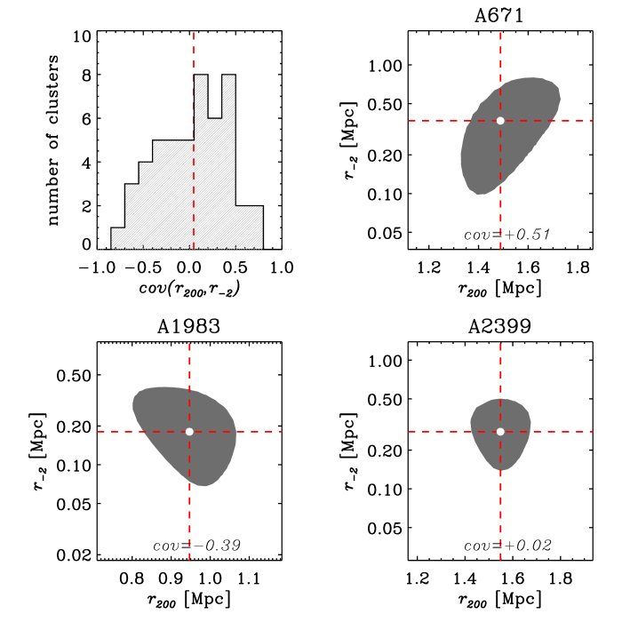
Figure 1: Top left panel: distribution of error covariance between the $r_{200}$ and $r_{-2}$ dynamical parameters. The mean of the distribution is indicated by a dashed vertical (red) line. Other panels: 68% confidence contours and best-fit values of the $r_{-2}$ (y-axis) vs. $r_{200}$ (x-axis) parameters of the MAMPOSSt analysis, in units of Mpc, for 3 of the 49 clusters analyzed. The best-fit solution is indicated by the dashed red lines and the white dot. The error covariance of the two parameters is listed at the bottom center of each panel.

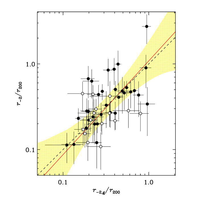
Figure 2: Scale radii of the total cluster mass density profiles, in units of the virial radii ($r_{-2}/r_{200}$ on the y-axis) vs. scale radii of the galaxy number density profiles, in the same units ($r_{\rm{-2,g}}/r_{200}$ on the x-axis). The error bars are 68% confidence levels, but do not include the uncertainties on $r_{200}$, given that the same quantity is used to normalize both variables on the two axes. The dashed line indicates the identity relation $r_{-2}\equiv r_{\rm{-2,g}}$. The solid (red) line indicates the best-fit log-log orthogonal relation between the two quantities, and the (yellow) shaded region indicates its 68% confidence region, obtained via the IDL code confidence_band. The best fit was obtained via the fitting procedure of Williams et al. (2010). Open (respectively filled) dots indicate clusters whose $n(R)$ has been fit with a pNFW (respectively King) model. A2124 is an outlier on this relation and its $[r_{\rm{-2,g}}/r_{200},r_{-2}/r_{200}]$ point lies off scale at $[5.5,0.23]$.

We compare the scale radii of the galaxy and the total mass distributions in Fig. 2. In this figure we show the best-fit values of $r_{-2}/r_{200}$ versus $r_{\rm{-2,g}}/r_{200}$ for our 49 clusters, where $r_{\rm{-2,g}}$ is the radius at which the logarithmic derivative of the 3D galaxy number density profile equals $-2$. For the pNFW model, $r_{\rm{-2,g}}=r_{\rm{g}}$, while for the King model, $r_{\rm{-2,g}}=\sqrt{2}r_{\rm{g}}$. The inverse of these quantities are the concentrations of the total mass and galaxy distributions, $c_{200}$ and $c_{{\rm g}}$, respectively. There is a very significant correlation between $r_{-2}/r_{200}$ and $r_{\rm{-2,g}}/r_{200}$ (Spearman rank correlation coefficient 0.51, corresponding to a probability of $2\times 10^{-4}$; see e.g., Press et al. 1992). A similar correlation has been noted before by van Uitert et al. (2016, see their Fig. 15) on a large sample of cluster $c_{200}$ values determined by a weak lensing stacking analysis.

We adopted the fitting procedure of Williams et al. (2010, see their Eqs. (3,4)), which is based on the minimization of $\chi^{2}$ defined by

$$\chi^{2}=\sum_{i=1}^{N}[y_{i}-(ax_{i}+b)]^{2}/\sigma_{i}^{2},$$ (9)

where the sum is over the $N=49$ clusters, $x$ and $y$ are the logarithms of the observational data, $\sigma^{2}=\sigma_{y}^{2}+a^{2}\sigma_{x}^{2}$, $a$ and $b$ are the intercept and slope of the fitted relation. Following Williams et al. (2010), if $\chi^{2}/{\rm dof}>1$, where dof is the number of degrees of freedom, 47 in our case (49 data - 2 free parameters), an additional extra scatter term, $\sigma_{\rm{int}}$, can be added in quadrature to $\sigma$, to lower the value of $\chi^{2}$/dof to unity. Such an extra scatter term represents the intrinsic scatter of the relation.

Since both x- and y-axis variables are affected by errors, and none of the two is dominating the observed scatter, we used the orthogonal distance regression (see Sect. 4.2 in Feigelson & Babu 1992). We find

$$\log(r_{-2}/r_{200})=(0.0\pm 0.1)+(1.1\pm 0.2)\times\log(r_{\rm{-2,g}}/r_{200})$$ (10)

with an intrinsic scatter around the relation of 0.23, which accounts for 90% of the total scatter. The mean ratio of the $r_{-2}/r_{\rm{-2,g}}$ values for the 49 clusters is $0.92\pm 0.08$, obtained using the robust biweight estimator of central location; we adopted this estimator in the rest of this paper as well (Beers et al. 1990). Our analysis therefore indicates that, on average, galaxies are spatially distributed like the total mass, in agreement with the result of Biviano & Girardi (2003, see their Fig. 9) taking into account that our analysis is restricted to the virial region. van Uitert et al. (2016) found instead $c_{{\rm g}}>c_{200}$, on average, but they only considered red sequence galaxies and these are known to be more centrally concentrated in clusters than the whole cluster population because of the well-known morphology-density relation (Dressler 1980).

4 Concentration-mass relation

In Fig. 3 we show $r_{-2}$ versus $r_{200}$ for our sample of 49 clusters. There is a significant correlation between the two quantities (Spearman rank correlation coefficient 0.45, corresponding to a probability 0.001). Using the fitting procedure of Williams et al. (2010) and taking the orthogonal relation, we find

$$\log r_{-2}=(-0.61\pm 0.08)+(1.3\pm 0.3)\times\log r_{200},$$ (11)

where both $r_{200}$ and $r_{-2}$ are in Mpc. From our data we measured $\chi^{2}/{\rm dof}<1$ without adding the extra scatter (see the first two lines of Table 2), which therefore remains undetermined. In other words, our observational uncertainties are too large to allow us to measure $\sigma_{\rm{int}}$.

We used the relation of Eq. (11) to derive the $cMr$,

$$\log c_{200}=(2.2\pm 1.4)-(0.11\pm 0.10)\times\log M_{200},$$ (12)

where $M_{200}$ is in $M_{\odot}$ units. Alternatively, we derived the $cMr$ by direct fitting of $c_{200}$ versus $M_{200}$ for our 49 clusters sample, using the procedure of Williams et al. (2010), and we find the orthogonal relation

$$\log c_{200}=(1.0\pm 1.4)-(0.03\pm 0.09)\times\log M_{200},$$ (13)

which is fully consistent with the relation of Eq. (12). We did not apply any correction for error covariance (Mantz et al. 2016) because there is no systematic error covariance for the $c_{200}$ and $M_{200}$ parameters in our cluster sample (see Sect. 3 and Fig. 1). The orthogonal scatter in the relation of Eq. (13) is 0.22, and also in this case it is dominated by observational uncertainties, since $\chi^{2}/{\rm dof}<1$ (see Table 2) without need for including the extra intrinsic scatter term $\sigma_{\rm{int}}$.

There is no significant correlation between $c_{200}$ and $M_{200}$ (Spearman rank correlation coefficient $-0.09$, corresponding to a probability 0.55), as expected given the flatness of the $cMr$ and the relatively large observational uncertainties. The $cMr$ of Eq. (13) is shown in Fig. 4, along with the $\{c_{200},M_{200}\}$ data points. In Fig. 5 we show the distribution of $c_{200}/c_{\rm{fit}}$, where $c_{\rm{fit}}$ is the best-fit concentration at given $M_{200}$ from Eq. (13). Figure 5 shows that the distribution is well fit by a lognormal curve, as expected theoretically (see, e.g., Jing 2000; Bullock et al. 2001; Dolag et al. 2004) with a dispersion of 0.22; this value is obtained from the $c_{200}$ versus $M_{200}$ fitting procedure.

Different model choices for $n(R)$ and $M(r)$ (see Sect. 3) have little effect on the $cMr$. We searched for systematic deviations from the $cMr$ of Eq. 13, by evaluating the $\chi^{2}$ as in Eq. (9) separately for different subsets of clusters. Specifically we considered the five subsets of clusters selected according to their best-fit $n(R)$ (King or pNFW) or $M(r)$ models (Bur, Her, or NFW). The derived $\chi^{2}$ values correspond to probabilities that imply no significant deviation from the $cMr$ of Eq. 13.

Since many previous determination of the $cMr$ have been obtained by adopting the NFW $M(r)$ model, we redetermined the $cMr$ by forcing this model to all our clusters, and we find the orthogonal relation

$$\log c_{200}=(1.2\pm 2.0)-(0.05\pm 0.14)\times\log M_{200},$$ (14)

fully consistent (albeit with larger scatter) with the $cMr$ of Eq. 13.

In Fig. 6 we compare the $cMr$ of Eq. (13) with other observational (top panel) and theoretical (bottom panel) estimates. The observational estimates of Groener et al. (2016) are based on several observational data and techniques, namely, weak and strong lensing (labeled, respectively, ’WL’ and ’SL’ in the figure), hydrostatic equilibrium applied to X-ray data (labeled ’X-ray’ in the figure), the Jeans equation (Łokas 2002; Łokas & Mamon 2003) or the Caustic technique (Diaferio & Geller 1997) applied to the projected phase-space distribution of galaxies in the cluster region (labeled LOSVD and CM in the figure, respectively). Other displayed observational $cMr$ are from Merten et al. (2015); Mantz et al. (2016); Okabe & Smith (2016) and based on weak+strong lensing, X-ray, and weak lensing data, respectively. The theoretical relations shown in Fig. 6 are from De Boni et al. (2013); Bhattacharya et al. (2013); Dutton & Macciò (2014); Correa et al. (2015b); Klypin et al. (2016). All $cMr$ are converted to an over-density of 200, when needed, assuming the NFW mass profile, and evaluated at a redshift $z=0.052$, which is the average redshift of our 49 clusters.

To estimate the level of agreement of the (theoretical or observational) $cMr$ shown in Fig. 6, with our own $\{c_{200},M_{200}\}$ data, we evaluate the goodness of the fits using Eq. (9). In that equation, to take into account the observational uncertainties of $cMr$ of other authors, we add in quadrature an additional scatter term, $\sigma_{+}$, derived from the uncertainties in the parameters of the different $cMr$, as given by their authors. We neglect the uncertainties in the parameters of the theoretical $cMr$; these are typically much smaller than the uncertainties in the parameters of the observational $cMr$. We list the $\sigma_{+}$, the resulting $\chi^{2}$/dof values, and their associated probabilities in Table 2. Our data favor a low-$c_{200}$ normalization of the $cMr$, close to the theoretical $cMr$ of De Boni et al. (2013), but they are also in agreement with the other theoretical relations shown in Fig. 6. On the other hand, many observational determinations of the $cMr$ disagree significantly with our data, except those of Merten et al. (2015) and Okabe & Smith (2016), and the LOSVD and SL relations of Groener et al. (2016).

Table 2: Comparison with observational and theoretical $cMr$

Reference	$\sigma_{+}$	$\chi^{2}$/dof	probability
Eq. (12)	–	0.88	0.70
Eq. (13)	–	0.88	0.70
Groener et al. (2016) CM	0.08	1.39	$0.04$
Groener et al. (2016) LOSVD	0.05	0.94	0.60
Groener et al. (2016) X-ray	0.02	1.61	$<0.01$
Groener et al. (2016) SL	0.12	1.14	$0.24$
Groener et al. (2016) WL	0.03	1.94	$<0.01$
Groener et al. (2016) WL+SL	0.03	3.09	$<0.01$
Mantz et al. (2016) X-ray	0.07	1.51	$0.01$
Okabe & Smith (2016) WL	0.15	0.46	$>0.99$
Merten et al. (2015) WL+SL	0.02	1.05	0.38
Correa et al. (2015b)	–	1.22	0.14
Dutton & Macciò (2014)	–	1.10	0.29
Bhattacharya et al. (2013)	–	1.09	0.33
Klypin et al. (2016)	–	0.93	0.61
De Boni et al. (2013)	–	0.91	0.65

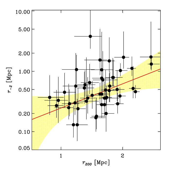
Figure 3: Scale-radii $r_{-2}$ vs. virial radii $r_{200}$, as obtained from the MAMPOSSt dynamical analysis, for the 49 clusters in our sample (Eq. (11)). Error bars indicate marginalized 68% confidence levels on the measured values. The solid (red) line indicates the best-fit log-log orthogonal relation between the two quantities, and the (yellow) shaded region its 68% confidence region, obtained using the IDL code confidence_band. The best fit was obtained using the fitting procedure of Williams et al. (2010).

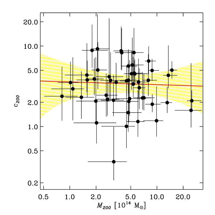
Figure 4: Concentration $c_{200}$ vs. mass $M_{200}$, as obtained from the MAMPOSSt dynamical analysis, for the 49 clusters in our sample (Eq. (13)). Error bars indicate 68% confidence levels on the measured values. The solid (red) line indicates the best-fit log-log orthogonal relation between the two quantities, and the (yellow) shaded region its 68% confidence region, obtained using the IDL code confidence_band. The best fit was obtained using the fitting procedure of Williams et al. (2010).

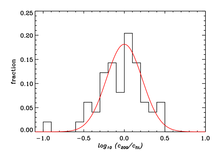
Figure 5: Distribution of $c_{200}/c_{\rm{fit}}$ for the 49 clusters in our sample, where $c_{\rm{fit}}$ is the best-fit concentration at given $M_{200}$ from Eq. (13). The red curve is a lognormal curve centered at $\log c_{200}/c_{\rm{fit}}=0$, with a scatter of 0.22, as obtained from the fitting procedure of Williams et al. (2010).

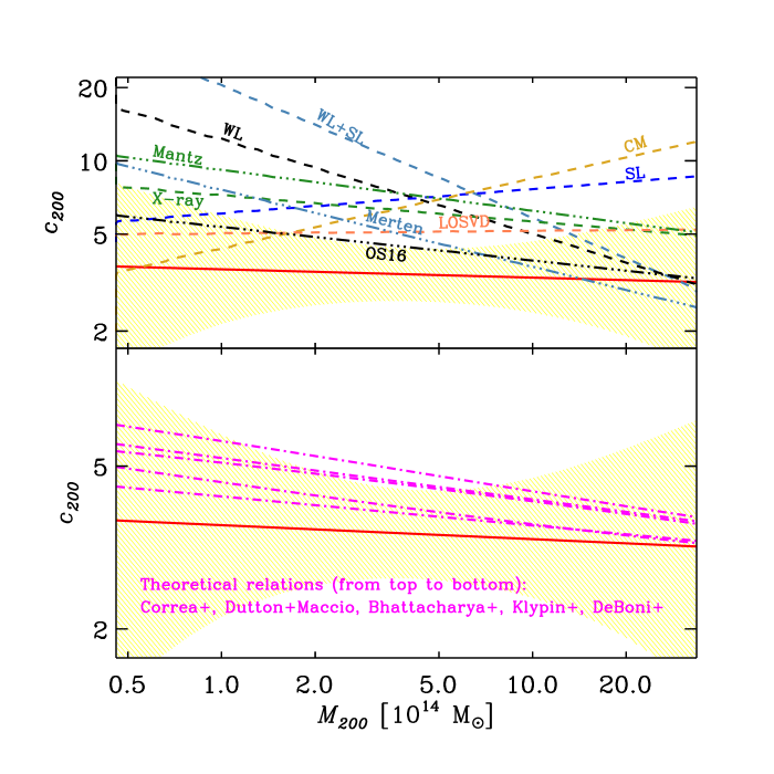
Figure 6: Best-fit $cMr$ from Eq. (13) and Fig. 4 (red solid line; yellow shading indicates the 68% confidence region), compared to other observational and theoretical $cMr$ determinations. Upper panel: comparison with other observational determinations of the $cMr$: Mantz et al. (2016, triple-dot-dashed green line labeled ’Mantz’), Merten et al. (2015, tripled-dot-dashed steel blue line, labeled ’Merten’), Okabe & Smith (2016, triple-dot-dashed black line, labeled ’OS16’), and Groener et al. (2016, dashed lines labeled as in Fig. 2 of their paper). Bottom panel: comparison with theoretical determinations of the $cMr$; from top to bottom: Correa et al. (2015b); Dutton & Macciò (2014); Bhattacharya et al. (2013); Klypin et al. (2016); De Boni et al. (2013).

5 Discussion

Using the WINGS and OmegaWINGS data sets (Fasano et al. 2006; Gullieuszik et al. 2015; Poggianti et al. 2016; Moretti et al. 2017), we have derived $c_{200}$ and $M_{200}$ for 49 nearby clusters with $\gtrsim 60$ cluster members with positions and redshifts (see Tables 1 and 1). The determination of $c_{200}$ and $M_{200}$ was obtained by application of the Jeans equation for dynamical equilibrium of a spherical gravitating system via the MAMPOSSt technique (Mamon et al. 2013). While not all clusters are expected to be fully dynamically relaxed, MAMPOSSt has also been shown to work reasonably well for partially relaxed clusters, in particular if the analysis is restricted to the virial region, as is the case here. To further reduce the effects of deviation from dynamical relaxation, before running MAMPOSSt, we removed from our sample those cluster members that were assigned a high probability of belonging to cluster substructures based on our new DS+ procedure described in Appendix A.

We find that mass and galaxies follow the same spatial distribution in clusters, even if these were not forced to be the same in our dynamical analysis. More specifically, we find that the scale radii (in units of $r_{200}$) of the galaxies and total matter distributions are correlated (see Fig. 2). This is the equivalent of saying that the galaxies and total mass spatial concentrations ($c_{{\rm g}}$ and $c_{200}$) are correlated, which is a result originally obtained by van Uitert et al. (2016). Not only do we find $c_{{\rm g}}$ and $c_{200}$ to be correlated, but we also find that $c_{{\rm g}}\approx c_{200}$ on average (see Eq. (10)). This finding confirms previous results (Carlberg et al. 1997; Mahdavi et al. 1999; Rines et al. 2001; Biviano & Girardi 2003). The scatter in the observed $r_{\rm{-2,g}}/r_{200}$ and $r_{-2}/r_{200}$ relation is however substantial and mostly intrinsic. We should therefore expect to find clusters where galaxies and the mass have different distributions (e.g., MACS1206, or LCDCS0504, see Biviano et al. 2013; Guennou et al. 2014, respectively), which is a warning against the temptation to assume $r_{-2}\equiv r_{\rm{-2,g}}$ as a general rule in future dynamical analyses.

We find a strong correlation between the MAMPOSSt-determined values of $r_{200}$ and $r_{-2}$ (see Fig. 3). Also in this case, the relation is almost linear (see Eq. (11)). As a consequence of the almost linear relation between $r_{200}$ and $r_{-2}$, $c_{200}\equiv r_{200}/r_{-2}$ is almost independent of $r_{200}$, and therefore – via Eq. (3) – also almost independent of $M_{200}$. In other words, the $cMr$ we obtain from the $r_{200}$ versus $r_{-2}$ best-fitting relation, is nearly flat (Eq. (12)). This $cMr$ is fully consistent with the $cMr$ we obtain directly from fitting $c_{200}$ versus $M_{200}$ (Eq. (13) and Fig. 4). We do not correct our $cMr$ for the $c_{200}$ and $M_{200}$ error covariance (Auger et al. 2013), since this is different for different clusters (see Sect. 3 and Fig. 1) and therefore unlikely to contribute a systematic trend in the $c_{200}$ versus $M_{200}$ diagram of the full sample of 49 clusters.

Our $cMr$ is in good agreement with theoretical predictions (see Fig. 6 and Table 2). In particular, the slope of our $cMr$ range from -0.12 to 0.06, and the value of $c_{15}$ (i.e., $c_{200}$ at the mass scale $M_{200}=10^{15}M_{\odot})$ ranges from 3.2 to 4.0. We therefore favor a low-normalization $cMr$ such as that of De Boni et al. (2013), but in fact all other theoretical $cMr$ considered in this paper (Bhattacharya et al. 2013; Dutton & Macciò 2014; Correa et al. 2015b; Klypin et al. 2016) are consistent with our data. In other words, our data confirm theoretical expectations about the $cMr$ of cosmological cluster-size halos, but are unable to discriminate among different models. In this sense, our results support the popular $\Lambda$CDM cosmological model for the formation and evolution of cluster-size halos, but do not constrain the parameters of this model to an accuracy comparable to that allowed by other independent, observational constraints such as those coming from cosmic microwave background observations (see, e.g. Correa et al. 2015b, and references therein).

The uncertainties in our derived values of $c_{200}$ and $M_{200}$ are too large to allow us to measure the intrinsic scatter in the $cMr$ we have determined (see Fig. 4 and Eq. (13)). We can only provide an upper limit to the intrinsic scatter in the $cMr$, that is the measured logarithmic scatter of 0.22 (0.51 in $\ln c_{200}$). Because this value is an upper limit, it is consistent with the scatter measured for the $cMr$ of halos from cosmological simulations ($\sim 0.2-0.3$; see, e.g., Jing 2000; Bullock et al. 2001; Dolag et al. 2004). Our observed distribution of $\log c_{200}/c_{\rm{fit}}$ is well represented by a lognormal function, in line with theoretical predictions (see, e.g., Jing 2000; Bullock et al. 2001; Dolag et al. 2004).

Even if our $cMr$ is not of sufficient quality to allow precision-cosmology determination of the cosmological parameters, the good agreement between our observed $cMr$ and $\Lambda$CDM theoretical parameters is very remarkable, given previous – even recent – claims of a significant tension between the observational constraints and the numerical predictions of the $cMr$ (e.g., Schmidt & Allen 2007; Comerford & Natarajan 2007; Fedeli 2012; Du et al. 2015; van Uitert et al. 2016). More specifically, observed $cMr$ have frequently been found to be steeper and of higher normalization than theoretical $cMr$. These discrepancies are evident from Fig. 6. In this figure, we compare our $cMr$ with several $cMr$ obtained from numerical simulations (Bhattacharya et al. 2013; De Boni et al. 2013; Dutton & Macciò 2014; Correa et al. 2015b; Klypin et al. 2016) and with other observational determinations of the $cMr$ based on X-ray data (Mantz et al. 2016), weak-lensing data (Okabe & Smith 2016), or a combination of weak- and strong-lensing data (Merten et al. 2015), and on a variety of data sets, including X-ray, weak- and strong-lensing, and projected-phase-space galaxy distributions (Groener et al. 2016). Most of these observational $cMr$ are steeper and/or have a higher normalization than the theoretical predictions. Three observational $cMr$ (labeled CM, LOSVD, and SL in Groener et al. 2016, and Fig. 6) have an unexpected inverted slope (i.e., $c_{200}$ increases with increasing $M_{200}$). Only the $cMr$ of Okabe & Smith (2016), based on weak-lensing data for 50 X-ray luminous clusters from LoCuSS (Okabe et al. 2013), is in excellent agreement with the theoretical predictions.

The comparison of our $cMr$ with other observational $cMr$ is quantified in Table 2. Since our $cMr$ is consistent with all the theoretical $cMr$, it is also inconsistent with those observational $cMr$ that are most different from the theoretical $cMr$. Our $cMr$ is instead in good or reasonable agreement with the observational $cMr$ of Okabe & Smith (2016) and Merten et al. (2015), respectively; the latter is based on strong- and weak-lensing data for clusters from the CLASH data set (Postman et al. 2012). Our $cMr$ is also consistent with the SL $cMr$ of Groener et al. (2016), but the agreement is due to the large uncertainties in the parameter values of this $cMr$.

Finally, it is particularly interesting to compare our $cMr$ with the CM and LOSVD $cMr$ of Fig. 6 and Groener et al. (2016). These two $cMr$ are both based on the analysis of the projected-phase space distributions of cluster galaxies. More specifically, the $c_{200}$ and $M_{200}$ values used for the CM $cMr$ are obtained by application of the Caustic method (Diaferio & Geller 1997; Diaferio 1999), while those used for the LOSVD $cMr$ are obtained by the Jeans analysis similar to our analysis here, but with different techniques (Łokas 2002; Łokas & Mamon 2003) from MAMPOSSt. The CM and LOSVD $cMr$ are based on 63, respectively 58, clusters (see Table 2 in Groener et al. 2016), that is, a similar statistics as our data set. The ’CM’ $cMr$ is statistically inconsistent with our $cMr$. This could be related to the known bias of the Caustic method that leads to over-estimating the cluster mass at small clustercentric distances, and thereby $c_{200}$ (Serra et al. 2011). On the other hand, the ’LOSVD’ $cMr$ is consistent with our $cMr$ (see Table 2).

6 Conclusions

We have derived the $cMr$ of 49 nearby clusters with data from the WINGS and OmegaWINGS surveys (Fasano et al. 2006; Cava et al. 2009; Gullieuszik et al. 2015; Poggianti et al. 2016; Moretti et al. 2017), by applying the MAMPOSSt technique (Mamon et al. 2013) to the projected-phase-space distributions of cluster members. We used particular care in defining cluster membership and developed a partially new methodology (described in Appendix A) to identify and remove cluster substructures before performing the dynamical analysis. While we did not force the mass distribution to be identical to the distribution of cluster galaxies in our analysis, this was indeed found to be the case, in an average sense, but with significant scatter from cluster to cluster.

Our $cMr$ was found to be consistent with theoretical predictions from $\Lambda$CDM cosmological simulations. The $c_{200}/c_{{\rm fit}}$ distribution was found to follow a lognormal distribution, as predicted theoretically. The quality of our $c_{200}$ and $M_{200}$ measurements is not sufficient to determine the intrinsic scatter of the $cMr$, nor to constrain cosmological parameters to the level required by the current precision cosmology. Nevertheless, we consider it remarkable that our $cMr$ slope and normalization are so close to the theoretical predictions, given that these have often been shown to be in tension with observational $cMr$ determinations, in the recent past. Only recently, more accurate $cMr$ determinations, based on gravitational lensing, appear to have overcome the discrepancy with the theoretical expectations and our $cMr$ is consistent with these $cMr$ determinations (Merten et al. 2015; Okabe & Smith 2016). Our $cMr$ is also consistent with the LOSVD $cMr$ of Groener et al. (2016), which – similar to our analysis for this work – is based on the Jeans dynamical analysis.

Our results thus support the $\Lambda$CDM hierarchical model of cosmological halos formation and evolution at least on the cluster scales. Our results show that the study of the $cMr$ of clusters can benefit from the dynamical analysis based on the projected-phase-space distribution of cluster galaxies, as a complement to other determinations based on X-ray and lensing techniques and data sets. In the future, we plan to extend this analysis to higher redshifts and to the lower end of the mass spectrum of galaxy systems.

Appendix A The DS+ method of identification of substructures

The method we developed for identifying cluster members belonging to substructures is an evolution of the classical method of Dressler & Shectman (1988), and we named it DS+ after the initials of the authors.

We start by describing the original test and how it has evolved in time. The original test looked for the differences $\delta$ of the mean velocity and velocity dispersion of all possible groups of $N_{{\rm g}}=11$ neighboring galaxies, from the corresponding cluster global quantities (see Eq. (1) in Dressler & Shectman 1988). When the sum of these differences, named $\Delta$, is much larger than the number of cluster members, $N_{{\rm m}}$, the cluster is likely to contain substructures. The likelihood is evaluated by Monte Carlo models in which cluster member velocities are randomly shuffled.

Bird (1994) proposed using $N_{{\rm g}}=N_{{\rm m}}^{1/2}$, instead of 11. Biviano et al. (2002) adopted this suggestion and further modified the original test by also considering the full $\delta$ distribution, rather than just the sum of the $\delta$s. The authors compared the observed $\delta$ distribution with Monte Carlo realizations obtained by azimuthally scrambling the galaxy positions, and identified statistically significant values of $\delta$, thus pinpointing the cluster members more likely to reside in substructures. An additional modification introduced by Biviano et al. (2002) was to consider only ’cold’ groups and to reject as spurious those groups with velocity dispersions larger than that of the whole cluster.

Ferrari et al. (2003) considered separately the differences in mean velocity and velocity dispersion, $\delta_{v}$ and $\delta_{\sigma}$, respectively. Girardi et al. (2015) evaluated $\delta_{\sigma}$ not with respect to the cluster global velocity dispersion, but with respect to the cluster velocity dispersion evaluated at the clustercentric distance of the group, thus introducing the use of the cluster velocity dispersion profile in the original method.

Our new DS+ method builds upon all these previous modifications of the original test of Dressler & Shectman (1988). Following Biviano et al. (2002) we adopted the following definitions for $\delta_{v},\delta_{\sigma}$,

$$\delta_{v}=N_{g}^{1/2}\,\mid\overline{v_{g}}\mid\,[(t_{n}-1)\,\sigma_{\rm{los}}(R_{g})]^{-1},$$ (15)

and

$$\delta_{\sigma}=[1-\sigma_{\rm{los,g}}/\sigma_{\rm{los}}(R_{g})]\,\{1-[(N_{g}-1)/\chi^{+}_{N_{g}-1}]^{1/2}\}^{-1},$$ (16)

where $N_{g}$ is the group multiplicity, $R_{g}$ is the average group distance from the cluster center, $\overline{v_{g}}$ is the mean group velocity, and the Student-$t$ and $\chi^{2}$ distributions are used to normalize the differences in units of the uncertainties in the mean velocity and velocity dispersion (as described in Beers et al. 1990), respectively. The mean velocity of the cluster is null by definition, since we work on cluster rest-frame velocities. Following Beers et al. (1990) we estimated the group and cluster velocity dispersions $\sigma_{\rm{los,g}}$ and $\sigma_{\rm{los}}$ using the biweight estimator for samples of at least 15 galaxies, and the gapper estimator for smaller samples.

The cluster line-of-sight velocity dispersion profile, $\sigma_{\rm{los}}(R)$, can in principle be directly estimated from the cluster member velocities. However, the result can be very noisy, even for cluster samples of $\sim 100$ members. We preferred to rely on a theoretical model. We obtained the cluster $\sigma_{\rm{los}}(R)$ by applying the Jeans equation of dynamical equilibrium and the Abel projection equation (Eqs. (8), (9), and (26) in Mamon et al. 2013), under the assumption of a NFW mass profile with $r_{200,i}$ estimated from the observed total cluster $\sigma_{v}$ (see Sect. 2.2), a concentration given by the relation of Macciò et al. (2008), and a velocity anisotropy profile modeled after the results of numerical simulations (Mamon et al. 2010). Given that $\sigma_{\rm{los}}$ vary slowly with $R$, the precise choice of the mass profile concentration has little impact on the results of our analysis.

We considered groups of several possible multiplicities, $N_{{\rm g}}(j)=j\times 3$, with $j=1,\ldots,k$, where $k$ is the lowest value of $j$ for which $N_{{\rm g}}(k)>N_{{\rm m}}^{1/2}$. In doing this we effectively take into account that substructures of different richness coexist in a given cluster. By considering only multiples of triplets we saved in computing time with little loss of generality.

The sums of each possible group $\delta$s, $\Delta_{v}\equiv\sum_{i=1}^{N_{{\rm g}}}\delta_{v}$, and $\Delta_{\sigma}\equiv\sum_{i=1}^{N_{{\rm g}}}\delta_{\sigma}$, are assigned probabilities via 500 MonteCarlo resamplings. In each of these, we replaced all the cluster galaxy velocities with random Gaussian draws from a distribution of zero mean and dispersion equal to $\sigma_{\rm{los}}(R_{g})$. Groups characterized by $\Delta_{v}$ and/or $\Delta_{\sigma}$ probabilities $\leq 0.01$, are considered significant.

To avoid the case of multiple group assignment for a given galaxy, we finally eliminated those groups that, even if significant, have one or more members in common with another group of higher significance (i.e., lower probability).

By the DS+ method we not only identified clusters with significant presence of substructures, but we identified the substructures themselves and the galaxies that belong to these substructures. To assess the accuracy of this new method, extensive tests are needed, using cluster-size halos extracted from cosmological simulations. These tests are currently underway and promising (Zarattini et al., in prep.) but a full analysis of them is beyond the scope of the present paper. In the future, we plan to perform a detailed analysis of the properties of OmegaWINGS cluster substructures and of their constituent galaxies.

References

- Adami et al. (1998) Adami, C., Mazure, A., Katgert, P., & Biviano, A. 1998, A&A, 336, 63
- Amodeo et al. (2016) Amodeo, S., Ettori, S., Capasso, R., & Sereno, M. 2016, A&A, 590, A126
- Ashman et al. (1994) Ashman, K. M., Bird, C. M., & Zepf, S. E. 1994, AJ, 108, 2348
- Auger et al. (2013) Auger, M. W., Budzynski, J. M., Belokurov, V., Koposov, S. E., & McCarthy, I. G. 2013, MNRAS, 436, 503
- Bartelmann (1996) Bartelmann, M. 1996, A&A, 313, 697
- Beers et al. (1990) Beers, T. C., Flynn, K., & Gebhardt, K. 1990, AJ, 100, 32
- Beers et al. (1991) Beers, T. C., Gebhardt, K., Forman, W., Huchra, J. P., & Jones, C. 1991, AJ, 102, 1581