Relative distribution of cosmic rays and magnetic fields

Abstract

Synchrotron radiation from cosmic rays is a key observational probe of the galactic magnetic field. Interpreting synchrotron emission data requires knowledge of the cosmic ray number density, which is often assumed to be in energy equipartition (or otherwise tightly correlated) with the magnetic field energy. However, there is no compelling observational or theoretical reason to expect such tight correlation to hold across all scales. We use test particle simulations, tracing the propagation of charged particles (protons) through a random magnetic field, to study the cosmic ray distribution at scales comparable to the correlation scale of the turbulent flow in the interstellar medium ($\simeq 100\,{\rm pc}$ in spiral galaxies). In these simulations, we find that there is no spatial correlation between the cosmic ray number density and the magnetic field energy density. In fact, their distributions are approximately statistically independent. We find that low-energy cosmic rays can become trapped between magnetic mirrors, whose location depends more on the structure of the field lines than on the field strength.

1 Introduction

Synchrotron emission is the main source of information about the nonthermal components of the interstellar and intergalactic medium (ISM and IGM). Its interpretation depends crucially on the relative distribution of magnetic fields and cosmic ray electrons. Cosmic rays tend to gyrate around magnetic field lines, so it is natural to expect some correlation between the cosmic ray and magnetic energy densities. On sufficiently long length- and time-scales, the cosmic ray distribution may achieve energy equipartition (Burbidge, 1956), or pressure balance, with the magnetic field (see review by Beck & Krause, 2005). Although the assumption of a tight, point-wise correlation between cosmic rays and magnetic fields across a wide range of scales lacks a compelling justification, it is often used in interpretations of synchrotron observations, regardless of the spatial resolution. Most of the energy of cosmic rays is carried by protons and heavier particles; therefore, such interpretations rely on an additional assumption that relativistic electrons are distributed similarly to the heavier cosmic ray particles.

The diffusivity of $5\,{\rm GeV}$ cosmic rays in a $5\,\mu{\rm G}$ magnetic field is believed to be about $10^{28}$–$10^{29}\,{\rm cm}^{2}\,{\rm s}^{-1}$, implying a diffusion length of the order of $1\,{\rm kpc}$ over the time scale of cosmic ray confinement in galaxies, $10^{6}\,{\rm yr}$ (Berezinskii et al., 1990). This suggests that the cosmic ray distribution will be significantly more uniform than that of the interstellar magnetic field, which varies strongly on scales smaller than $0.1\,{\rm kpc}$ (Ruzmaikin et al., 1989; Beck et al., 1996). However, cosmic rays are more tightly confined to field lines where the field is strongest, and so we might still expect some positive correlation between cosmic ray density and magnetic energy on small scales. On the other hand, overall pressure balance can, equally plausibly, lead to local anticorrelation between cosmic ray and magnetic energy densities (Beck et al., 2003). Indeed, from a comparison of the observed and modelled magnitude of the fluctuations in synchrotron intensity in the Milky Way and nearby spiral galaxies, Stepanov et al. (2014) suggested that cosmic ray electrons and interstellar magnetic fields are slightly anticorrelated at scales $\lesssim 100\,{\rm pc}$.

Large-scale simulations of cosmic ray propagation in the advection-diffusion approximation rely on various (often crude) parameterisations of the diffusion tensor and its dependence on the magnetic field. Using a fluid description of cosmic rays in nonlinear dynamo simulations, assuming anisotropic (but constant) diffusion coefficients, Snodin et al. (2006) found no correlation between magnetic field and cosmic ray energy densities. Such simulations may be appropriate at scales exceeding the diffusion length (of order $1\,{\rm kpc}$), but not at the smaller scales that are relevant in the present study. For a typical cosmic ray proton, with energy $1$–$10\,{\rm GeV}$, in a $5\,\mu{\rm G}$ magnetic field, the Larmor radius is about $10^{-6}$–$10^{-5}\,{\rm pc}$, which is much smaller than the correlation length of magnetic field ($50$–$100\,{\rm pc}$) or the diffusion length of cosmic rays (which is of the order of $1\,{\rm kpc}$). Thus, the small-scale structure of the magnetic field will be particularly important for the propagation of cosmic rays in this energy range.

In this paper, we use test particle simulations to explore, in detail, the spatial distribution of cosmic ray particles propagating in a random magnetic field. Whereas previous test particle simulations have been mostly concerned with the calculation of the cosmic ray diffusion coefficient, we primarily consider the spatial distribution of cosmic rays and its relation to the magnetic field. Our model is kinematic, i.e., we only consider the effect of the magnetic field on the cosmic rays and neglect any effects of cosmic ray pressure on the gas flow and hence on the magnetic field. In Section 2 we describe the numerical model for random magnetic fields and in Section 3 we present our model for simulating cosmic ray propagation. Our results on cosmic ray density and its relation to the magnetic field are presented in Section 4. We conclude in Section 5 and suggest further avenues for study.

2 Implementation of random magnetic fields

The propagation of cosmic rays is sensitive to rather subtle details of the magnetic field in which they move. The spectrum provides a complete statistical description of a Gaussian random magnetic field, so it must also determine the corresponding cosmic ray diffusivity for a given energy of particle. The propagation of cosmic rays in an isotropic Gaussian random magnetic field (for which the probability distribution function of each vector component is Gaussian) has been the subject of many studies (Berezinskii et al., 1990; Michalek & Ostrowski, 1997; Giacalone & Jokipii, 1999; Casse et al., 2002; Schlickeiser, 2002; Parizot, 2004; Candia & Roulet, 2004; DeMarco et al., 2007; Globus et al., 2008; Shalchi, 2009; Plotnikov et al., 2011; Harari et al., 2014; Snodin et al., 2016; Subedi et al., 2017). However, radio (Gaensler et al., 2011; Haverkorn & Spangler, 2013), submillimeter (Zaroubi et al., 2015) and neutral hydrogen (Heiles & Troland, 2005; Kalberla & Kerp, 2016) observations suggest that the magnetic field in the ISM is strongly non-Gaussian, spatially intermittent, and filamentary. Such an intermittent field is also expected theoretically, as a result of turbulent dynamo action (Wilkin et al., 2007) and random shock compression (Bykov & Toptygin, 1985, 1987; Bykov, 1988). The magnetic field generated by dynamo action in galaxy clusters is also likely to be intermittent (Ruzmaikin et al., 1989; Subramanian et al., 2006). The presence of magnetic intermittency can significantly affect the propagation of cosmic rays (Shukurov et al., 2017). In non-Gaussian fields, the separation and size of magnetic structures may play an important role (Shukurov et al., 2017), especially for low energy particles. In this section, we describe the magnetic fields that are used in our analysis of cosmic ray propagation. A discussion of the structure of small-scale interstellar magnetic field can be found in Appendix A. Throughout the text, the small-scale or fluctuating field is represented by $\mathbf{b}$, the large-scale (or mean) field by $\mathbf{B_{0}}$ and the total field by $\mathbf{B}=\mathbf{b}+\mathbf{B_{0}}$.

2.1 Magnetic fields generated by a random flow

For our numerical study, we use a random magnetic field produced by kinematic fluctuation (small-scale) dynamo action. Using a triply-periodic cubic box of length $L$, with $512^{3}$ grid points, we solve the induction equation

$$\frac{\partial\mathbf{b}}{\partial t}=\nabla\times(\mathbf{u}\times\mathbf{b})+\eta\nabla^{2}\mathbf{b},$$ (1)

where $\mathbf{u}(\mathbf{x},t)$ is a prescribed velocity field and $\eta$ is the magnetic diffusivity, which we take to be constant. To ensure $\nabla\cdot\mathbf{b}=0$, we numerically solve for the corresponding magnetic vector potential. We define the magnetic Reynolds number to be $R_{\mathrm{m}}=l_{0}u_{0}/\eta$, where $l_{0}$ is the outer scale of the turbulent velocity flow and $u_{0}$ is the root-mean-square (rms) velocity. Dynamo action occurs, i.e., the magnetic field grows exponentially, if $R_{\mathrm{m}}$ exceeds a critical magnetic Reynolds number, $R_{\mathrm{m,c}}$, whose value depends on the velocity field.

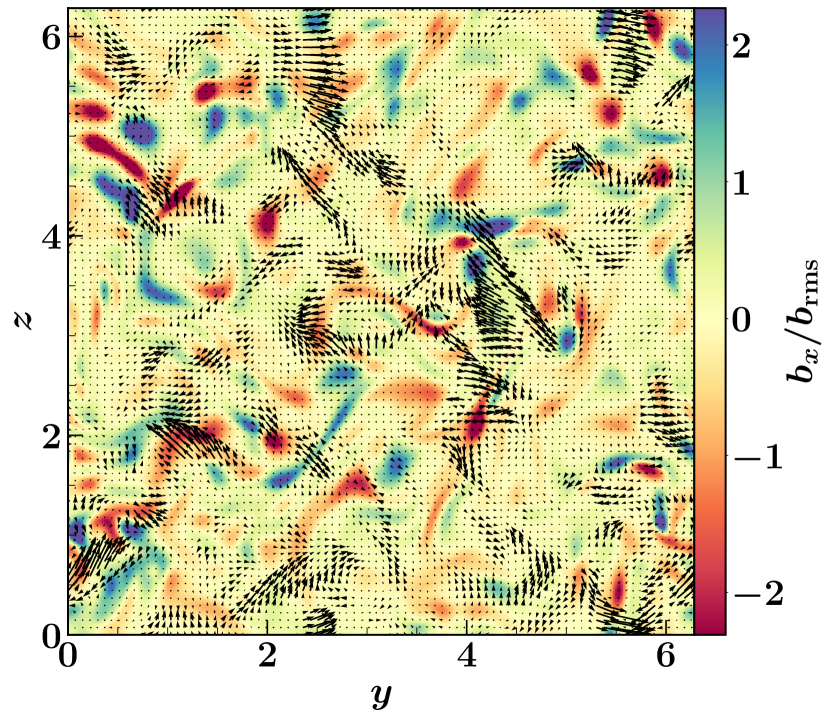
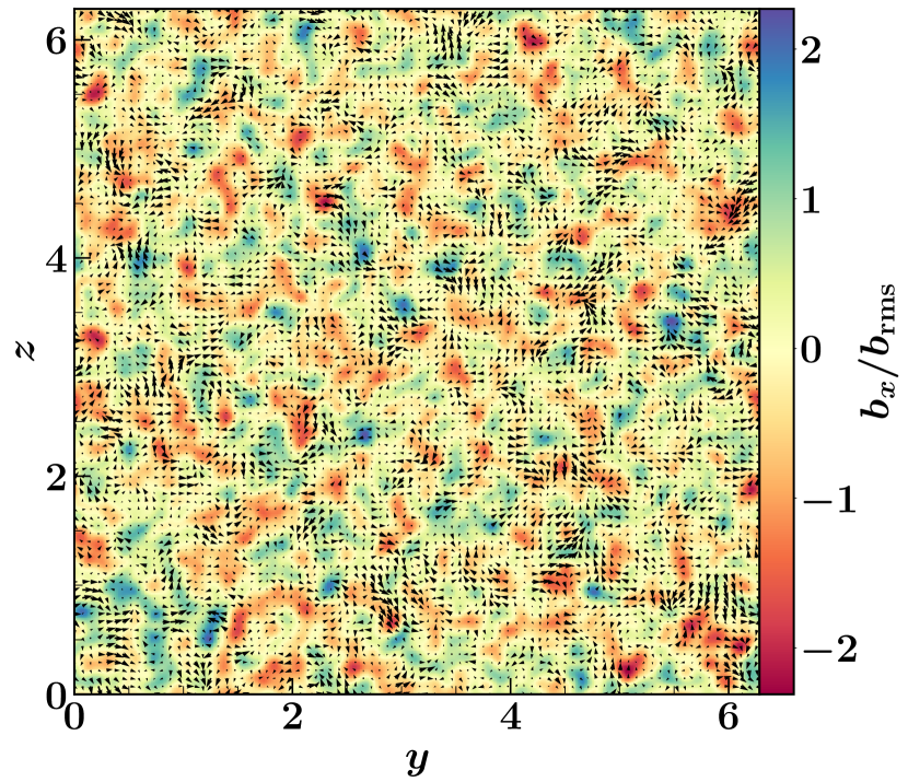
Figure 1: 2D cut in the $yz$–plane through the middle of the domain with vectors for $(b_{y}/\,b_{\rm rms},b_{z}/\,b_{\rm rms})$ and colours showing the magnitude of $b_{x}/\,b_{\rm rms}$ for intermittent (left) and randomized (right) magnetic fields. For intermittent magnetic field the colours are saturated for both positive and negative values to match the scale of the randomized field (see the $x$-axis of Fig. 3 for the actual difference in numbers). The intermittent magnetic field is more ordered and stronger in the filaments whereas the randomized field lacks such structures.

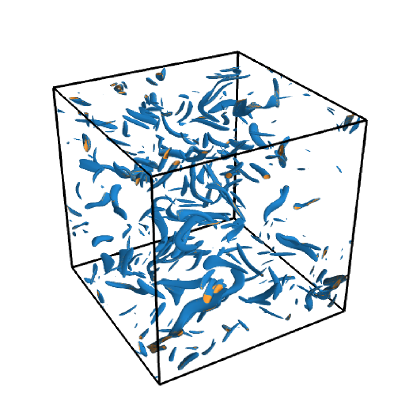
Figure 2: The figure shows isosurfaces of $b^{2}/\,b_{\rm rms}^{2}=12$ (blue) and $b^{2}/\,b_{\rm rms}^{2}=15$ (yellow) for the dynamo-generated magnetic field at $R_{\mathrm{m}}=3182$. It is intermittent, showing long filaments with large gaps between filaments.

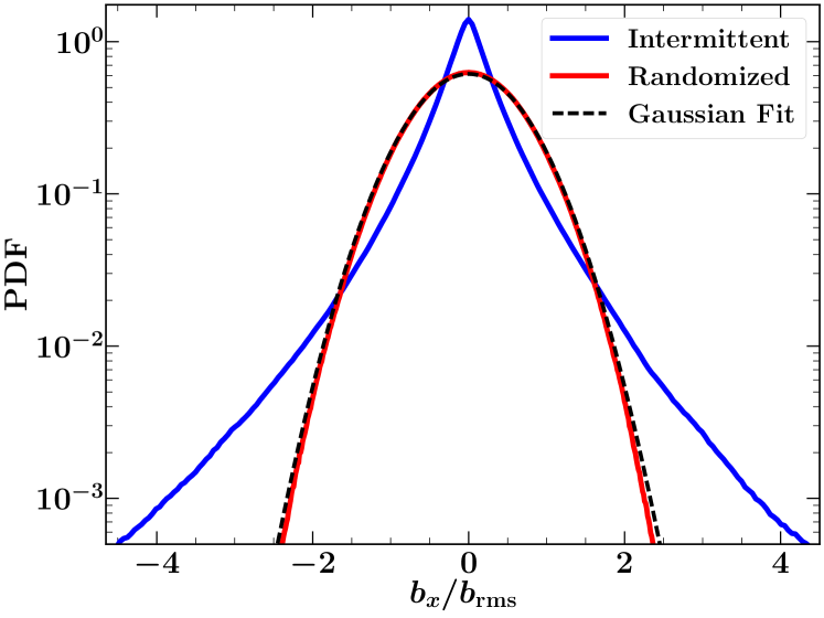
Figure 3: The figure shows PDFs of $b_{x}/\,b_{\rm rms}$ for intermittent (blue) and randomized (red) magnetic fields. Both have zero mean but the intermittent magnetic field has long tails whereas the randomized field (obtained by Fourier phase randomization) has a Gaussian PDF (dashed).

We construct the velocity field, $\mathbf{u}$, by superposing Fourier modes with a range of wavenumbers, $k$, and a chosen energy spectrum $E(k)$, using the same prescription as Fung et al. (1992) and Wilkin et al. (2007):

$$\mathbf{u}(\mathbf{x},t)=\sum_{n=0}^{N-1}\left[\mathbf{C}_{n}(\mathbf{k}_{n})\cos\phi_{n}+\mathbf{D}_{n}(\mathbf{k}_{n})\sin\phi_{n}\right],$$ (2)

where $\phi_{n}=\mathbf{k}_{n}\cdot\mathbf{x}+\omega_{n}t$, $\mathbf{k}_{n}$ is a randomly oriented wavevector of magnitude $k_{n}$, and $\omega_{n}=[k_{n}^{3}E(k_{n})]^{1/2}$ is the frequency at that scale. The vectors $\mathbf{C}_{n}(\mathbf{k}_{n})$ and $\mathbf{D}_{n}(\mathbf{k}_{n})$ have random directions in the plane perpendicular to $\mathbf{k}_{n}$, so that the flow is incompressible ($\nabla\cdot\mathbf{u}=0$). Their magnitudes determine the power spectrum $E(k)$, and are chosen such that $E(k)\propto k^{-5/3}$ and the rms velocity is $u_{0}$. We chose $N=40$ with $\mathbf{k}_{n}$ such that the flow is periodic, and with distinct $k_{n}$ between $2\pi/L$ to $8\pi/L$, where $L=2\pi$ is the width of our domain which is also equal to the outer scale, $l_{0}$, of the velocity flow. This flow acts as a dynamo if $R_{\mathrm{m}}>R_{\mathrm{m,c}}\simeq 1000$, and produces a spatially intermittent magnetic field, as can be seen in the left-hand panel of Fig. 1 and Fig. 2.

The presence of structures in the magnetic field affects the propagation of cosmic rays, especially for low energy particles. For such particles, intermittency enhances cosmic ray diffusion (Shukurov et al., 2017). Here we are interested in exploring the correlation between the magnetic field and cosmic rays. The intermittent nature of this dynamo-generated magnetic field provides an excellent test case for this study since there are localized regions of strong magnetic field.

We also consider a Gaussian random magnetic field having the same power spectrum $M_{b}(k)$ as the intermittent magnetic field. Such a Gaussian random field is obtained as follows: First, a spatial Fourier transform of the intermittent magnetic field is taken and then each complex mode is multiplied with a random phase. Then taking an inverse Fourier transform gives a Gaussian randomized magnetic field with unchanged $M_{b}(k)$, but where coherent structures have been destroyed (Chapter 7 in Biskamp, 2003; Snodin et al., 2013; Shukurov et al., 2017). The structural difference between intermittent and Gaussian random magnetic field is illustrated in Fig. 1 which shows the magnetic fields in a 2D cut through the middle of the numerical domain, with colours showing the third component. Figure 2 shows the filamentary structure of the intermittent magnetic field (at $b^{2}/\,b_{\rm rms}^{2}$ of order ten). The probability distribution function (PDF) of a single component of both the intermittent and randomized field is shown in Fig. 3. The intermittent field has long heavy tails, whereas the randomized field has a Gaussian probability distribution.

2.2 Large-scale magnetic field

The ISM contains both fluctuating (small-scale) and mean (large-scale) magnetic fields (Chapter 5 in Klein & Fletcher, 2015; Beck et al., 1996; Beck, 2016). The large-scale component is correlated over several $\,{\rm kpc}$ whereas the small-scale component has a correlation length less than the correlation scale of turbulence ($\lesssim 0.1\,{\rm kpc}$). The small-scale and the large-scale components of the magnetic field contain comparable energies. By comparing large-scale magnetic field models (with resolution of $\sim 75\,{\rm pc}$) of a spiral galaxy with observations, Moss et al. (2007) found that a spatially uniform distribution of cosmic rays was better at matching the observations than an equipartition assumption between cosmic rays and large-scale magnetic field. This suggest that the cosmic rays may not be correlated with large-scale magnetic field.

To explore the effects of a large-scale magnetic field on the propagation of cosmic rays, we add a uniform mean field directed along the $x$-axis to the random magnetic field as described in Section 2.1. We consider several values for the ratio of the mean field $B_{0}$ to the random field, $\,b_{\rm rms}$, up to $B_{0}/\,b_{\rm rms}=3$.

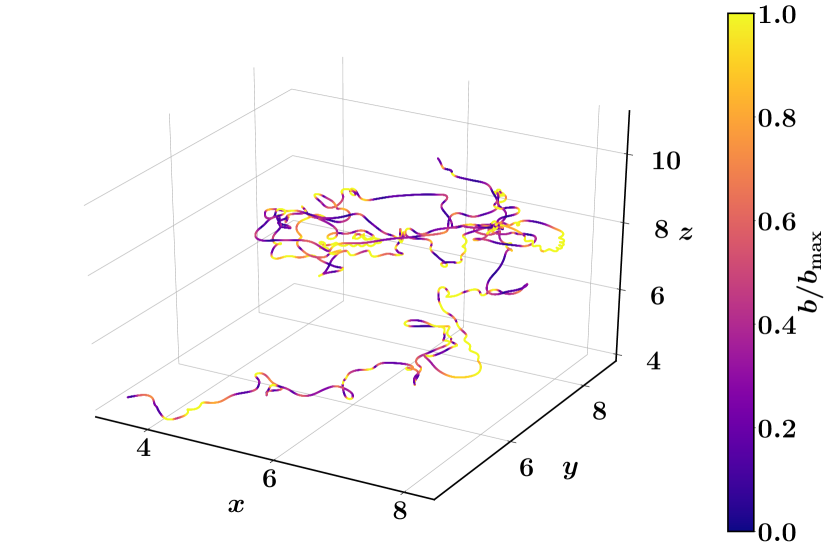
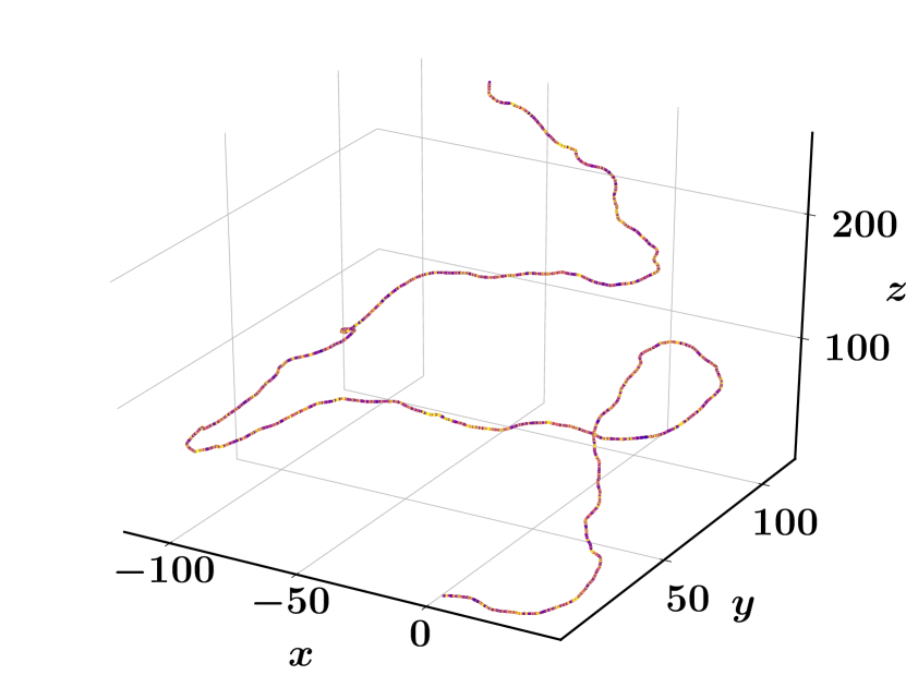
Figure 4: Single particle trajectories for $r_{\text{L}}/l_{0}=0.011$ (left-hand panel) and $0.318$ (right-hand panel) in the intermittent magnetic field of the left-hand panel of Fig. 1 and Fig. 2. Colours shows the strength of the magnetic field along the trajectory normalized to its maximum value along the part of trajectory shown. For $r_{\text{L}}/l_{0}=0.011$, the particle path is more tangled than for $r_{\text{L}}/l_{0}=0.318$ where the particle motion is almost ballistic between rare scattering events.

3 Cosmic ray propagation

The propagation of cosmic rays in random magnetic fields is largely determined by the ratio between the Larmor radius $r_{\text{L}}$ of the particle gyration and the length scale $l_{b}$ of magnetic field variations, e.g., its correlation length. The Larmor radius and Larmor frequency of a relativistic particle of rest mass $m$ and charge $q$, travelling at a speed $v$ in a magnetic field of strength $B$, are given by

$$r_{\text{L}}=\frac{\gamma mcv}{qB}\qquad\mbox{and}\qquad\omega_{0}=\frac{v}{r_{\text{L}}},$$ (3)

respectively, where $\gamma=\left(1-v^{2}/c^{2}\right)^{-1/2}$ is the Lorentz factor, and $c$ is the speed of light in a vacuum. The correlation length $l_{b}$ of an isotropic random field with power spectrum $M_{b}(k)$ is defined as (Monin & Yaglom, 1971)

$$l_{b}=\frac{\pi}{2}\frac{\int_{0}^{\infty}k^{-1}M_{b}(k)\,\mathrm{d}k}{\int_{0}^{\infty}M_{b}(k)\,\mathrm{d}k}.$$ (4)

The correlation length of a magnetic field produced by the fluctuation dynamo action is significantly smaller than $l_{0}$, at least in the kinematic stage where $l_{b}/l_{0}$ is of order $R_{\mathrm{m}}^{-1/2}$ (Kazantsev, 1967; Zeldovich et al., 1990; Schekochihin et al., 2004; Brandenburg & Subramanian, 2005). For $R_{\mathrm{m}}=3182$, we have $l_{b}/l_{0}\approx 0.0244$.

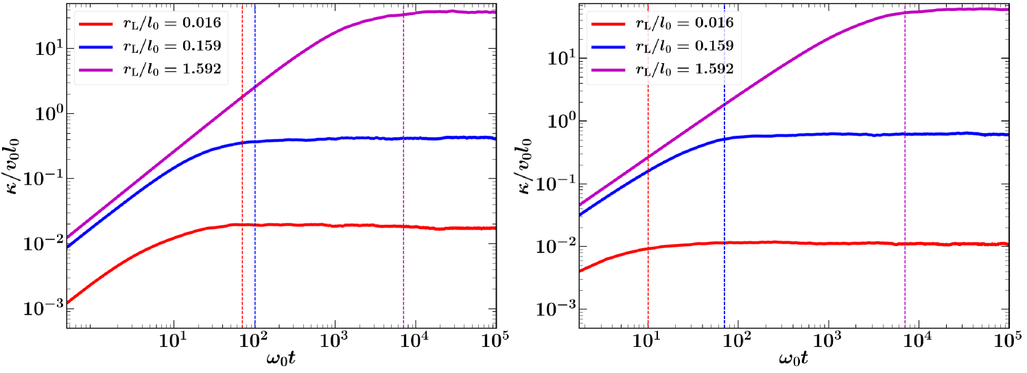
Figure 5: Normalized cosmic ray diffusivity $\kappa/v_{0}l_{0}$ as a function of normalized time $\omega_{0}t$ for $r_{\text{L}}/l_{0}=0.016,0.159,1.592$ for the intermittent (left) and randomized (right) magnetic fields shown in Fig. 1. Here $\omega_{0}=v_{0}/r_{\text{L}}$ is the Larmor frequency based on $\,B_{\rm rms}$. The dashed lines of the corresponding colours show the time $\,t_{\rm d}$ after which the propagation becomes diffusive: $\kappa(t)\approx\kappa$ at $t>\,t_{\rm d}$. For low energy particles ($r_{\text{L}}\leq l_{b}$), the diffusivity in the intermittent magnetic field is larger than in the randomized (Gaussian) field of identical power spectrum.

3.1 Test particle simulations of cosmic rays

We consider relativistic charged particles propagating in a static magnetic field, $\mathbf{B}(\mathbf{x})$. The trajectory of each particle satisfies

$$\frac{\mathrm{d}^{2}\mathbf{r}}{\mathrm{d}t^{2}}=\frac{v_{0}}{r_{\text{L}}}\,\displaystyle\frac{\mathrm{d}\mathbf{r}}{\mathrm{d}t}\times\frac{\mathbf{B}}{\,B_{\rm rms}},$$ (5)

where $\mathbf{r}$ is the particle’s position, $v_{0}$ is its speed, $\mathbf{B}/\,B_{\rm rms}$ is the total magnetic field normalized to its rms value $\,B_{\rm rms}$, and $r_{\text{L}}$ is the Larmor radius (defined with respect to $\,B_{\rm rms}$). The time-scale over which interstellar magnetic fields change significantly is of the order of the eddy turnover time in interstellar turbulence, $10^{7}\,{\rm yr}$ (Beck et al., 1996). This time-scale is longer than the (diffusive) confinement time of cosmic rays in galaxies, which is of the order of $10^{6}\,{\rm yr}$ (Berezinskii et al., 1990). It is therefore customary to neglect any time dependence of the magnetic field in Eq. (5) and, correspondingly, neglect any electric fields (e.g., Giacalone & Jokipii, 1999; Casse et al., 2002). This means that the speed of each particle remains constant. This is equivalent to neglecting particle acceleration, a process physically distinct from diffusive particle propagation (which is the focus of this article) which is due to scattering of cosmic ray particles by magnetic inhomogeneities. Since we consider static magnetic field, the diffusive reacceleration (Strong et al., 2007; Grenier et al., 2015), which is due to moving magnetic inhomogeneities, is also neglected.

We solve Eq. (5) numerically for an ensemble of cosmic ray particles (specifically, $8192$), all of the same speed $v_{0}$, but giving each a random initial position and velocity direction. The initial conditions are chosen randomly, and are uniformly distributed over all positions and directions, but do not very uniformly fill the magnetic field cube, due to there only being a finite number of particles. For a given energy of particle, we find the smallest Larmor time ($2\pi/\omega_{0}$) based on the maximum magnetic field in the domain and then fix the time step as $0.001$ times the smallest Larmor time, to ensure that we carefully resolve all particle gyrations. We also check that the energy is conserved (as far as is permitted by the numerical scheme) throughout the total propagation time $T$. For a given magnetic field configuration, the nature of the trajectories depends only on the parameter $r_{\text{L}}/l_{0}$, which is indicative of the particle energy, as illustrated in Fig. 4. By construction, the static magnetic field through which the particle propagates is periodic in all three directions, with period $L=2\pi$. Even though the magnetic field is periodic, the particle trajectories are not: they enter and leave the domain at different points. There is an important distinction between the Eulerian frame of the computational domain and the Lagrangian frame moving with each particle. Whilst the magnetic field is periodic in the Eulerian sense, there is no periodicity in the magnetic field along each particle trajectory (however many times the particle enters and leaves the domain).

A high-energy particle, with $r_{\text{L}}\gg l_{b}$, is typically deflected by only a small angle of order $l_{b}/r_{\text{L}}$ over a distance $l_{b}$ and its trajectory is, therefore, rather insensitive to the structural properties of the magnetic field at scales smaller than $r_{\text{L}}$. By the central limit theorem, the statistical properties of an ensemble of cosmic ray particles become Gaussian after a large number of such deflections. Particles of smaller energies, $r_{\text{L}}\lesssim l_{b}$, are more sensitive to the fine structure of the magnetic field, and it is not obvious how the spatial distribution of such cosmic rays will be related to the magnetic energy density, especially given that their diffusion tensor is sensitive to magnetic intermittency (Shukurov et al., 2017). In particular, the distribution of cosmic rays may be intermittent in a spatially intermittent magnetic field. Figure 4 shows the trajectories of particles of low and high energy (left- and right-hand panels, respectively). The latter move faster (note the different axis scales in the two panels) and, at the scale of the left-hand panel, the trajectory of the higher-energy particle is nearly straight almost everywhere.

The random nature of the magnetic field makes the particle propagation diffusive at sufficiently large spatial and temporal scales. Without a mean field, the propagation is isotropic. We therefore calculate the isotropic diffusion coefficient as the limit of the finite-time diffusivity $\kappa(t)$,

$$\kappa=\lim_{t\to\infty}\kappa(t),\qquad\kappa(t)=\frac{1}{6t}\langle|\mathbf{r}(t)-\mathbf{r}(0)|^{2}\rangle,$$ (6)

where the angular brackets denote averaging over the ensemble of particles. Figure 5 shows $\kappa(t)$ for the two magnetic fields shown in Fig. 1, one intermittent and the other statistically Gaussian, and for several values of $r_{\text{L}}/l_{0}$. In each case there is an initial phase of ballistic particle motion, in which $\kappa(t)$ is approximately linear in $t$, followed by a diffusive phase where $\kappa(t)$ settles to its asymptotic value. The start of the diffusive phase, $\,t_{\rm d}$, is the time when the slope of $\kappa(t)$ becomes small, $\mathrm{d}\kappa/\mathrm{d}(\omega_{0}t)\simeq 10^{-6}$; this time is indicated by a vertical dashed line in Fig. 5.

To obtain the number density of cosmic rays, $n_{\rm cr}$, from the test particle simulations we calculate the coordinates of each particle modulo $L=2\pi$, i.e., relative to the periodic magnetic field. Next, we divide the periodic domain into $512^{3}$ cubes and count the number of particles within each cube. The size of the cubes was chosen to match the spatial resolution of the magnetic field, which was obtained from a dynamo simulation on a $512^{3}$ grid, but we have checked that the results are not very sensitive to the exact size of the cubes. The result is the instantaneous number density of the particles $\tilde{n}(\mathbf{x},t)$. We then average the density of particles within each cube over a sufficiently long period $T$ ($\gg\,t_{\rm d}$), to obtain the cosmic ray density $n_{\rm cr}(\mathbf{x})=(T-\,t_{\rm d})^{-1}\int_{\,t_{\rm d}}^{T}\tilde{n}(\mathbf{x},t^{\prime})\,\mathrm{d}t^{\prime}$. We have checked that the results are not dependent on the sampling time ($\mathrm{d}t^{\prime}$) as long as it is smaller than a few times the Larmor time ($2\pi/\omega_{0}$). But for lower sampling rate the simulation has to be averaged over a longer total time (higher $T$) to collect sufficient statistics. We note that different energies were simulated over different periods $T$ to obtain roughly the same $\langle{n_{\rm cr}(\mathbf{x})}\rangle$ for all energies.

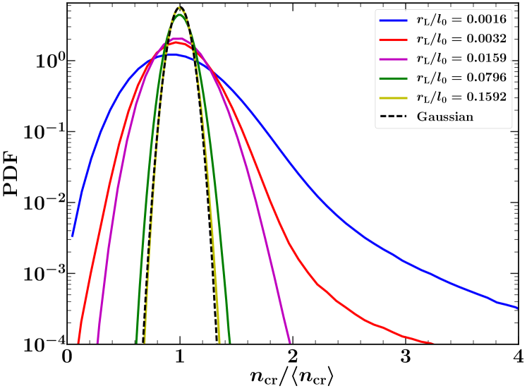
Figure 6: Probability density function (PDF) of the relative number density of cosmic ray particles, $n_{\rm cr}/\langle n_{\rm cr}\rangle$, for various $r_{\text{L}}/l_{0}$ in intermittent (left panel) and randomized (Gaussian) magnetic fields (right panel), with no mean-field and no pitch angle scattering (PAS). Long tails are a signature of intermittent structures in the cosmic ray distribution. For high-energy particles, the distribution is nearly Gaussian (with width increasing as energy decreases) in both intermittent and Gaussian magnetic fields, but below a certain energy ($r_{\text{L}}\lesssim l_{b}$) long tails develop. A black dashed line shows the PDF of a random variable drawn from a Gaussian distribution with unit mean value and standard deviation of $0.07$.

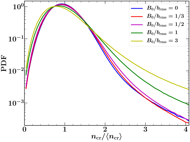
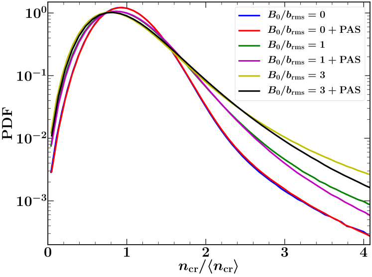
Figure 7: PDF of $n_{\rm cr}/\langle n_{\rm cr}\rangle$ for $r_{\text{L}}/l_{0}=0.0016$ in the intermittent field of Fig. 2 with an imposed mean field of various magnitudes $B_{0}$ (left-hand panel) and with the pitch angle scattering further included (right-hand panel). Intermittency in the cosmic ray distribution increases as the mean field becomes stronger, especially for $B_{0}/\,b_{\rm rms}\geq 1$, manifested in heavier tails at larger $n_{\rm cr}/\langle n_{\rm cr}\rangle$. The pitch angle scattering enhances diffusion and thus decreases the level of intermittency.

3.2 Magnetic field at the Larmor scale

Cosmic ray particles are especially sensitive to magnetic fluctuations at a scale comparable to their Larmor radius. As described by Kulsrud (2005), when a cosmic ray particle encounters such a magnetic fluctuation, its pitch angle $\theta$ defined via

$$\mu\equiv\cos\theta=\frac{\displaystyle\mathbf{v}\cdot\mathbf{B}}{\displaystyle|\mathbf{v}||\mathbf{B}|}\,,\qquad\mathbf{v}=\displaystyle\frac{\mathrm{d}\mathbf{r}}{\mathrm{d}t}\,,$$ (7)

changes by

$$\delta\theta=-\pi\frac{\delta B}{B}\cos\chi\,,$$ (8)

where $\delta B/B$ is the ratio of the fluctuation amplitude at the Larmor scale to the local mean magnetic field (i.e., the field averaged over a scale significantly larger than $r_{\text{L}}$), and $\chi$ is the relative phase between the cosmic ray velocity vector and the wavevector of the magnetic fluctuation with which the particle interacts.

Magnetic fluctuations at the Larmor scale can be a part of a magnetic energy spectrum that extends from larger scales or be excited by cosmic rays themselves via the streaming instability (Kulsrud & Pearce, 1969; Wentzel, 1974; Kulsrud, 2005). The latter are usually referred to as ‘self-generated waves’. The scattering due to magnetic fluctuations at the Larmor scale is referred to as pitch angle scattering, and Desiati & Zweibel (2014) stress its importance for cosmic ray diffusion. The magnitude of the magnetic fluctuations that are associated with pitch angle scattering due to self-generated waves is estimated in Appendix B as $\delta B/B\simeq 10^{-2}$ in the hot interstellar gas.

The spectrum of hydromagnetic turbulence in the ISM extends to very small scales. Schekochihin et al. (2009) suggest that the spectrum of kinetic Alfvén waves is truncated by dissipation at scales as small as the thermal electron Larmor radius, which is approximately $3\times 10^{6}\,{\rm cm}$ in the warm ionized ISM. This scale is much smaller than the Larmor radius of the relativistic particles of cosmic rays. However the spectrum of Alfvén wave turbulence is rather steep: $k^{-5/3}$ at larger scales (above $1\,{\rm pc}$ – Brandenburg & Subramanian, 2005) where the gas is collisional and, at smaller scales, $k_{\parallel}^{-2}$ for the perturbations parallel to the magnetic field (which matter for the cosmic ray scattering – Farmer & Goldreich, 2004). For such steep spectra, the relative magnitude of the magnetic fluctuations at the Larmor radius of a $5\,{\rm GeV}$ particle is of the order of $\delta B/B\simeq 10^{-4}$, which is negligible in comparison with the self-generated waves.

Within our model the magnetic field is imposed and the streaming instability cannot occur. We therefore parametrize the cosmic ray scattering by self-generated waves. This is done by rotating the velocity vector of each particle every Larmor time ($2\pi/\omega_{0}$) by an angle given by Eq. (8), with $\delta B/B=10^{-2}$ and $\chi$ uniformly distributed between $0$ and $2\pi$. Throughout the text, this is referred to as pitch angle scattering (PAS).

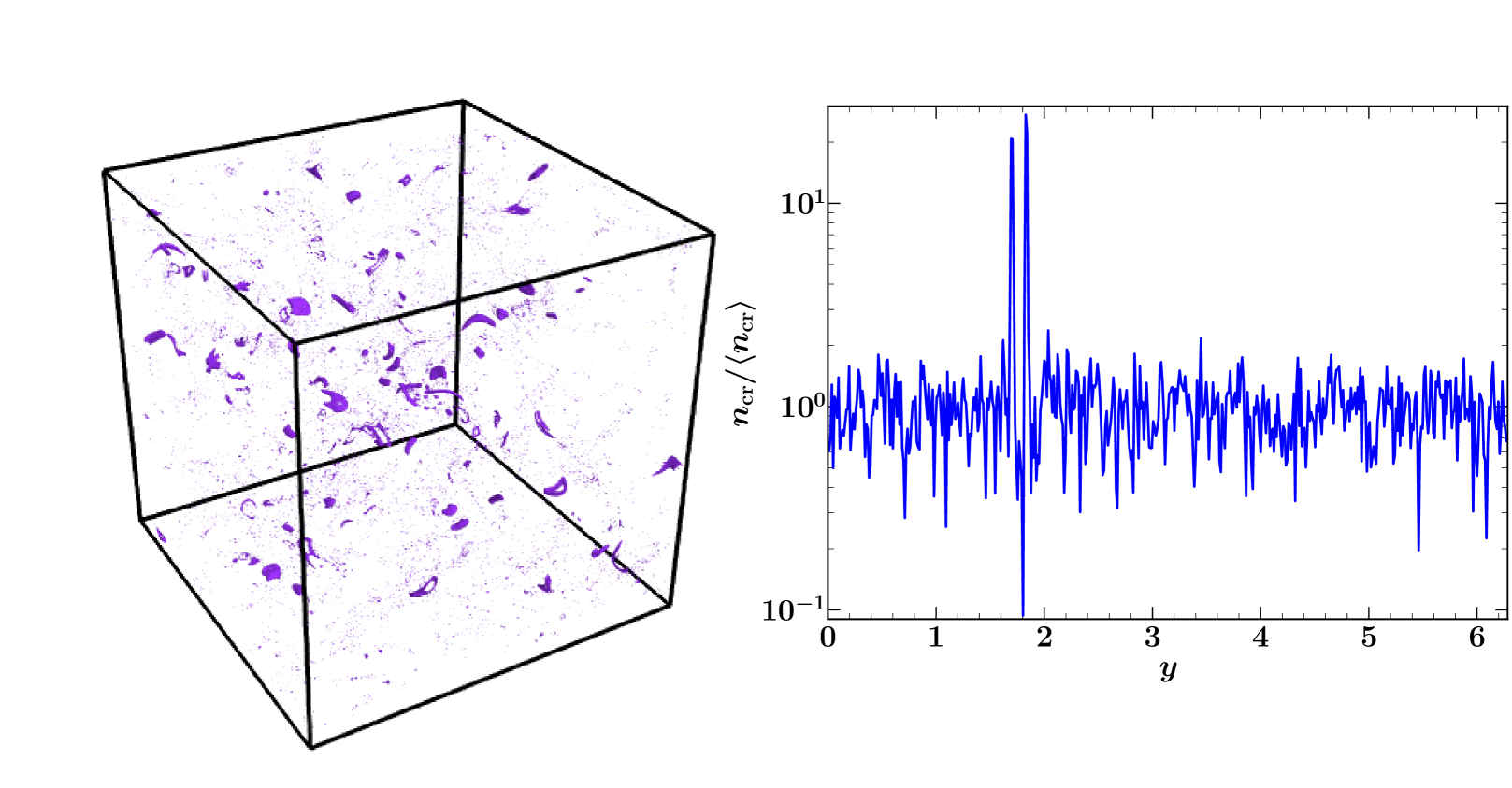
Figure 8: Isosurfaces of the number density of cosmic rays at $n_{\rm cr}/\langle n_{\rm cr}\rangle=3.5$ for $r_{\text{L}}/l_{0}=0.0016$ in an intermittent magnetic field showing a highly inhomogeneous distribution (left-hand panel). The right-hand panel shows the variation of the relative number density of the particles along the straight line $(x,z)=(\pi,3.97)$, characterized by rare, strong maxima against a weakly fluctuating background.

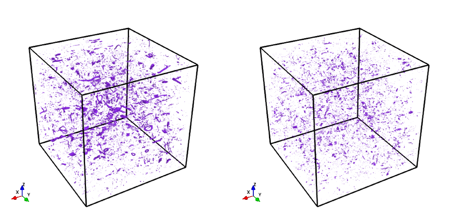
Figure 9: Isosurfaces of the number density of cosmic rays at $n_{\rm cr}/\langle n_{\rm cr}\rangle=3.5$ for $r_{\text{L}}/l_{0}=0.0016$ in an intermittent magnetic field with an imposed mean field of a strength $B_{0}/\,b_{\rm rms}=1$ aligned with the $x$-axis (left-hand panel) and with pitch angle scattering further added (right-hand panel).

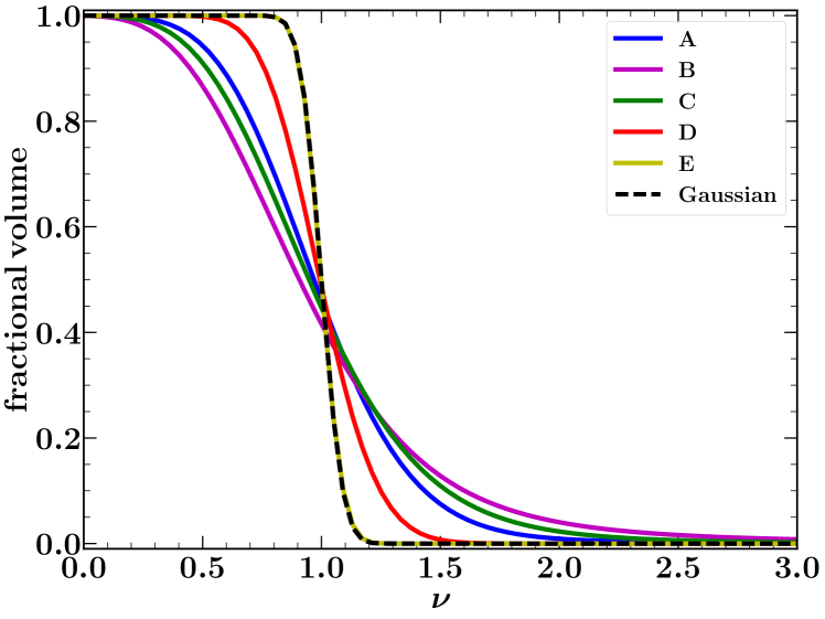
Figure 10: The fractional volume of cosmic ray structures with $n_{\rm cr}/\langle n_{\rm cr}\rangle\geq\nu$ for Models A–E of Table 1. A black dashed line shows the fractional volume for a random variable drawn from a Gaussian distribution with unit mean value and standard deviation of $0.07$.

Table 1: Representative selection of simulations, summarising the effects of particle energy, magnetic field structure and pitch angle scattering (PAS). All quantities are defined in the text.

Model	$r_{\text{L}}/l_{0}$	$\mathbf{b}$	$B_{0}/\,b_{\rm rms}$	PAS	$f$
A	$0.0016$	Intermittent	0	no	0.81
B	$0.0016$	Intermittent	1	no	0.68
C	$0.0016$	Intermittent	1	yes	0.84
D	$0.0016$	Randomized	0	no	0.96
E	$0.1592$	Intermittent	0	no	0.99

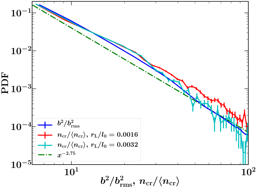
Figure 11: PDF of intermittent magnetic field energy density normalized to its rms value, $b^{2}/\,b_{\rm rms}^{2}$, and the number density of cosmic rays normalized to its mean, $n_{\rm cr}/\langle n_{\rm cr}\rangle$, for $r_{\text{L}}/l_{0}=0.0016,0.0032$. All three of them have power-law tails and the same exponent. Statistical errors are considerable at probability densities below about $\leq 5\times 10^{-5}$.

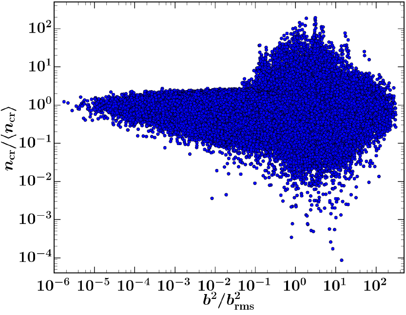
Figure 12: The scatter plot of cosmic ray number density, $n_{\rm cr}/\langle n_{\rm cr}\rangle$ and magnetic energy density, $b^{2}/\,b_{\rm rms}^{2}$, in intermittent magnetic field for $r_{\text{L}}/l_{0}=0.0016$.

4 Results

Figure 6 shows the probability density function (PDF) of the particle number density $n_{\rm cr}$ obtained in intermittent and randomized (Gaussian) magnetic fields. For cosmic rays of relatively high energy ($r_{\text{L}}/l_{b}>1$ or $r_{\text{L}}/l_{0}>0.0244$), the number density $n_{\rm cr}$ is very nearly uniform in space, and its PDF is Gaussian. At lower energies, the PDF has a long, heavy tail, which signifies the presence of spatially localized structures in the cosmic ray distribution. It is remarkable that the distribution of cosmic rays is intermittent in both intermittent and Gaussian magnetic fields. The PDF of $n_{\rm cr}$ on including mean magnetic fields of various strength, with (right-hand panel) and without (left-hand panel) particle pitch angle scattering is shown in Fig. 7. Here too, for low energies the cosmic ray number density distribution has a long tail.

4.1 Spatial intermittency of cosmic rays

Cosmic rays fill all the volume available. However, the distribution for low energy cosmic rays (especially for $r_{\text{L}}/l_{0}=0.0016$ or $r_{\text{L}}/l_{b}\simeq 0.06$) is not homogeneous. Random magnetic fields produce cosmic ray distributions where a significant fraction of the volume is occupied by strong particle concentrations. The PDFs of $n_{\rm cr}$ shown in Fig. 6 have a Gaussian core and a heavy tail, a manifestation of the spatial intermittency. The core contains most of the particles and has $n_{\rm cr}$ close to its mean value. The tail represents rare but intense small-scale spatial structures. Figure 8 shows the number density of cosmic rays, obtained as described in Section 3.1, in the intermittent magnetic field shown in the left-hand panel of Fig. 1 and Fig. 2. The distribution is inhomogeneous and evidently sensitive to the magnetic field structure. The distribution of cosmic rays is affected by both the mean magnetic field and pitch angle scattering. As shown in Fig. 7, the mean magnetic field enhances the intermittency in the cosmic ray distribution, whereas pitch angle scattering reduces it. Fig. 9 illustrates how the shape and number of structures in the cosmic ray distribution are affected. With a mean field, the structures are more numerous and many extend along the mean field direction, aligned with the $x$-axis in the example shown. This effect becomes significant when $B_{0}/\,b_{\rm rms}\geq 1$. On the other hand, pitch angle scattering enhances cosmic ray diffusion and, consequently, reduces their intermittency, as shown in the right-hand panel of Fig. 9. The degree of intermittency can be measured in terms of the parameter $f=\langle n_{\rm cr}\rangle^{2}/\langle n_{\rm cr}^{2}\rangle$ (see Table 1). For high energy particles, $r_{\text{L}}/l_{0}=0.1592$ or $r_{\text{L}}/l_{b}\simeq 6.52$, $f$ is close to unity, indicating a homogeneous particle distribution. This feature of the cosmic ray distribution is further detailed in Fig. 10 where we show the dependence of the fractional volume of a region where $n_{\rm cr}/\langle n_{\rm cr}\rangle\geq\nu$ on $\nu$ for the configurations of Table 1. Particles of sufficiently high energy, $r_{\text{L}}/l_{b}\gg 1$, are not sensitive to the fine structure of the magnetic field and the probability distribution of their number density is Gaussian. The dependence of the fractional volume, shown in Fig. 10, on the presence of the mean magnetic field and its change due to pitch angle scattering confirms that the spatially intermittency increases on including mean field and decreases on including pitch angle scattering. Figure 11 shows the PDF of magnetic field energy density and cosmic ray distribution for the tail region (values higher than the mean for each of the distributions). Both distributions are power laws and the exponent for the magnetic field roughly matches that for the cosmic ray number density. The cosmic ray distribution for low energy particles is intermittent with heavy power law tails.

4.2 Statistical relation between magnetic field and cosmic rays

The simplest measure of a relation between cosmic rays and magnetic field is their cross-correlation coefficient,

$$C(n_{\rm cr},B^{2})=\frac{\overline{n_{\rm cr}B^{2}}-\overline{n}_{\mathrm{cr}}\overline{B^{2}}}{\sigma_{n_{\rm cr}}\sigma_{B^{2}}}\,,$$ (9)

where the overbar denotes an average over the whole domain, and $\sigma$ is the standard deviation of the quantity specified in the subscript. The value of $C$ ranges from $C=1$ for perfect correlation to $C=-1$ for perfect anti-correlation. In all cases considered, we find that the two distributions are uncorrelated, $C\approx 0$. This is true even for the lowest-energy cosmic rays considered ($r_{\text{L}}/l_{0}=0.0016$), despite the fact that they are closely confined to magnetic lines. The correlation does not emerge even when the cosmic ray density and magnetic field are smoothed to a coarser spatial grid. To confirm that this behaviour is not an artefact of the initial conditions used for the cosmic ray particles, we have also performed a simulation with their initial positions in the regions of the strongest magnetic field shown in Fig. 2. The value of $C$ in this case is very close to unity initially but vanishes quickly, within the time $\,t_{\rm d}$.

Figure 12 shows the scatter plot of the cosmic ray number density and magnetic field energy density, whose form confirms that the two variables are uncorrelated. We also confirm that cosmic rays and magnetic field distributions are statistically independent. As demonstrated in Appendix C (where more details can be found), the joint probability distribution function of cosmic rays and magnetic field distributions, $p(n_{\rm cr},b^{2})$, can be factorized as follows:

$$p(n_{\rm cr},b)\approx(1.6+9.9\mathrm{e}^{-10.5b^{2}/\,b_{\rm rms}^{2}})\mathrm{e}^{-(n_{\rm cr}/\langle n_{\rm cr}\rangle-1)^{2}/0.18}\,,$$ (10)

for the intermittent magnetic field and

$$p(n_{\rm cr},b)\approx 0.5(b^{2}/\,b_{\rm rms}^{2})^{-1}\mathrm{e}^{-0.3\ln(b^{2}/\,b_{\rm rms}^{2})^{2}}\mathrm{e}^{-(n_{\rm cr}/\langle n_{\rm cr}\rangle-0.9)^{2}/0.32}\,,$$ (11)

for the randomized (Gaussian) magnetic field. In both cases, the joint PDF is separable which illustrates that the cosmic rays and magnetic field distributions are independent in the diffusive regime of the cosmic rays.

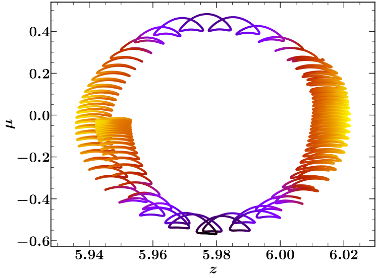
Figure 13: The left-hand panel shows a particle trajectory with magnetic field strength along the trajectory shown with colour. The dark grey lines show magnetic field lines near the trajectory. The particle moves forward and backward between two magnetic mirrors. The right-hand panel shows the angle between the particle velocity vector and the $z$-axis with magnetic field strength colour coded. The particle turns around ($\mu$ changes sign) at the magnetic mirrors, regions where magnetic field is stronger.

4.3 Random magnetic traps

Since $n_{\rm cr}$ is not correlated with the magnetic field strength, the regions of high cosmic ray density must instead be caused by some geometrical property of the magnetic field lines. In fact, we find that these regions occur where cosmic rays become trapped between two magnetic mirrors, i.e., positions where magnetic lines converge. As shown in Fig. 13, if a magnetic flux tube is pinched at both ends, then particles are repeatedly reflected between the two ends, creating a ‘magnetic trap’. Because the field lines must be reasonably smooth in order to form a trap, the regions of high cosmic ray density are typically smaller than the magnetic correlation length, $l_{b}$. The cosine of the particle’s pitch angle, $\mu$, defined in Eq. (7), is shown in the right-hand panel of Fig. 13 as a function of position and magnetic field strength. This quantity reverses sign along the trajectory whenever the particle is reflected at an end of the magnetic trap. This happens where the magnetic field is relatively strong. Magnetic trapping is associated with the conservation of $v_{\perp}^{2}/B$, an adiabatic invariant (Jackson, 1998), where $v_{\perp}=v\sin\theta$ is the particle speed perpendicular to the local magnetic field. We have verified that $v_{\perp}^{2}/B=\text{const}$ with relative accuracy of order $10^{-5}$ along the trajectories of the trapped particles.

We estimate the enhancement of cosmic ray number density due to magnetic traps as follows. Consider a magnetic trap of a length $l$ in a magnetic flux tube of a radius $d$. For an ensemble of particles within the trap, the expected trapping time $\tau$ is $d^{2}/\kappa_{\perp}$, where $\kappa_{\perp}$ is the local transverse diffusivity of cosmic rays. Defining $N$ to be the number of times that a particle travels along the trap before leaving it, we expect $N\sim\tau v/l$. The resulting number density of particles within the trap is given by $n_{0}=N\overline{n}_{\mathrm{cr}}$ with $\overline{n}_{\mathrm{cr}}$ the mean number density of cosmic rays. The number density of the particles within the trap follows as

$$n_{0}\simeq\frac{vd^{2}}{l\kappa_{\perp}}\overline{n}_{\mathrm{cr}}.$$ (12)

According to this order of magnitude estimate, we therefore expect that the number of trapped particles will depend inversely upon the local cosmic ray diffusivity as well as upon the size and number of traps.

A mean magnetic field introduces a specific direction which particles follow and so increases the probability for a magnetic trap to occur, as shown in the left-hand panel of Fig. 9. On the other hand, the pitch angle scattering due to self-generated waves decreases the level of intermittency in the cosmic ray number density, as shown in the right-hand panel of Fig. 9, because it facilitates the transverse diffusion. When the distribution on the right-hand panel of Fig. 9 is smoothed over a coarser scale, it does not correlate with the distribution on the left-hand panel of Fig. 9. This further illustrates that the pitch angle scattering not only reduces the length of trapping region but also changes the propagation of particles significantly.

It is important to note that the spatial intermittency of cosmic rays does not require the intermittent structure of the random magnetic field. Even in the randomized magnetic field, which has an almost perfect Gaussian statistics and is free of intermittency, magnetic traps occur and lead to a spatial intermittency of cosmic rays.

5 Conclusions and discussion

Using test particle simulations of cosmic ray propagation, we have demonstrated that the spatial distribution of cosmic rays is not correlated with magnetic field strength on spatial scales that are less than (or comparable to) the outer scale, $l_{0}$, of a random flow that produces magnetic field. This implies that the local equipartition between cosmic ray and magnetic field energy densities does not occur on these scales. In fact, we find that cosmic ray number density and magnetic field are approximately statistically independent.

At high energies, $r_{\text{L}}>l_{b}$ with $l_{b}$ the correlation length of the magnetic field, the cosmic ray distribution is uniform. At low energies, $r_{\text{L}}<l_{b}$, the spatial distribution of cosmic rays is intermittent in both Gaussian and non-Gaussian (spatially intermittent) magnetic fields. This occurs because of the presence of magnetic traps in random magnetic fields where the local magnetic field has a specific structure but is not necessarily strong. As a result, the cosmic ray number density is not directly related to the local magnetic field strength.

The trapping, and the ensuing intermittency in the cosmic ray distribution, are enhanced by a mean magnetic field and reduced by the pitch angle scattering of cosmic ray particles or any other additional diffusion. The number density of cosmic ray particles within the traps depends on the size of the trap and the transverse diffusivity of cosmic rays with respect to the local magnetic field. Statistical properties of the traps (such as their rate of occurrence, size, etc.) are controlled by subtle properties of the random magnetic field; it appears that finding them is a non-trivial probabilistic problem.

For cosmic rays to become trapped, their Larmor radius must be smaller than the correlation length of the magnetic field, i.e., $r_{\text{L}}\leq l_{b}$. In spiral galaxies, where $l_{b}\lesssim 100\,{\rm pc}$, the proton energy in a $5\,\mu{\rm G}$ field with $r_{\text{L}}=100\,{\rm pc}$ is $10^{8}\,{\rm GeV}$. Thus, the trapping of cosmic rays described above should be effective and efficient for galactic cosmic rays. In galaxy clusters, with $l_{b}\lesssim 10\,{\rm kpc}$ and $b\simeq 1\,\mu{\rm G}$, protons of energy up to $10^{9}\,{\rm GeV}$ can be trapped and thus exhibit spatial intermittency. This particle trapping can effectively confine higher energy particles for which other confinement mechanisms (scattering by self-generated waves, magnetic field structure, field line random walk) are not very active (Chandran, 2000).

The lack of correlation between cosmic rays and magnetic field in galaxies at small scales (below a few kiloparsecs) is suggested by analyses of the radio–far-infrared correlation (Hoernes et al., 1998; Berkhuijsen et al., 2013; Basu & Roy, 2013). Here we have presented a physical reason for that. Energy equipartition (or pressure balance) between cosmic rays and magnetic field may yet hold at scales much larger than the driving scale of turbulence, $l_{0}\simeq 100\,{\rm pc}$ in spiral galaxies and $10\,{\rm kpc}$ in galaxy clusters.

The assumption of energy equipartition between cosmic rays and magnetic fields, and related assumptions of their pressure balance or minimum energy, are routinely used in interpretations of synchrotron observations (Beck & Krause, 2005; Arbutina et al., 2012; Beck, 2016, and references therein). Apart from assuming that the cosmic ray energy density, dominated by protons, is related to the local magnetic energy density, these interpretations also rely on a fixed ratio of the number densities of cosmic ray electrons and protons and presume that the electrons and protons are identically distributed in space. We have shown that local, small-scale energy equipartition between cosmic rays and random magnetic field does not occur. The spatial distribution of cosmic ray energy is sensitive to the geometry of magnetic field rather than its strength. However, the distribution of cosmic ray electrons responsible for synchrotron emission must be modelled separately with allowance for their synchrotron and inverse-Compton energy losses. We expect that the distribution of cosmic ray electrons would differ significantly from that of protons, plausibly exhibiting stronger intermittency since the electrons would spend more time in magnetic traps as they lose their energy. This would mean that equipartition-type estimates are even less reliable when applied to the local energy densities. It cannot be excluded, however, that the spatial distributions of cosmic ray and magnetic field energy densities are related at larger scales of order kiloparsec, comparable to the diffusion length of cosmic ray particles over their confinement time. We shall discuss elsewhere this version of the equipartition arguments.

The intermittency in the distribution of cosmic ray particles discussed above is a robust feature of their propagation in a random magnetic field that emerges in both Gaussian and non-Gaussian magnetic fields. This extreme small-scale inhomogeneity may affect interactions of cosmic rays with interstellar gas (Grenier et al., 2015, and references therein), including spallation reactions and ionization, e.g., producing strong local variations in the ionization rate. The $\gamma$-ray emissivity can also be affected by the trapping of cosmic rays particles in random magnetic traps. Quantifying the effect of cosmic ray intermittency on these and other observables (such as spectra) will require energy losses to be included in the model, which we aim to do in the future.The effects of intermittency in the cosmic ray distribution may be numerous and require a careful, systematic study.

Test particle simulations are constrained by the need to resolve the Larmor radius and period of the particle gyration. For this reason, it is not practical to model those particles of energies of order GeV that contribute most to the energy density of cosmic rays if the magnetic field structure is to be resolved in full. For example, the Larmor radius of a $5\,{\rm GeV}$ proton in a $5\,\mu{\rm G}$ ISM magnetic field is $10^{8}$ times smaller than $100\,{\rm pc}$, the typical scale of the magnetic field. Our conclusions are based on an extrapolation of the results obtained for particles of effectively much larger energies. Then modelling of cosmic ray propagation at lower energies requires a fluid model based on a variant of the diffusion-advection equation but with the diffusion tensor that allows for the non-trivial structure of the magnetic field. Such modelling is beyond the scope of this paper but remains our high priority.

6 Acknowledgments

We are grateful to Ellen Zweibel, Prateek Sharma and Pasquale Blasi for useful discussions. We thank the anonymous referee for her/his helpful suggestions and comments. This work was supported by the STFC (ST/N000900/1, Project 2), the Leverhulme Trust (RPG-2014-427) and the Thailand Research Fund (RTA5980003).

Appendix A Fine structure of interstellar magnetic fields

Several mechanisms produce the random magnetic fields in the interstellar medium. Tangling of the large-scale magnetic field by turbulent flows produces a volume-filling random field whose statistical properties are controlled by the turbulence. This magnetic field is a byproduct of the large-scale (mean-field) dynamo action. If the turbulent velocity has Gaussian statistical properties, the resulting random magnetic field is also a Gaussian random field. Random motions can also generate a random magnetic field directly through the small-scale (fluctuation) dynamo action. The resulting magnetic field is spatially intermittent (magnetic field concentrated in filaments and ribbons) and has strongly non-Gaussian statistical properties (Zeldovich et al., 1990; Schekochihin et al., 2004; Brandenburg & Subramanian, 2005; Wilkin et al., 2007). Another similarly structured contribution is produced by compression in random shock fronts driven by supernova explosions (Bykov & Toptygin, 1985; Federrath et al., 2010). The result of such compression is a complex random magnetic field represented by both Gaussian and non-Gaussian parts that scatter cosmic rays differently (Zelenyi et al., 2015; Shukurov et al., 2017). In this section we estimate the contribution of each of the above mechanisms to the small-scale interstellar magnetic fields. For clarity, we denote $\mathbf{b}_{1}$, $\mathbf{b}_{2}$ and $\mathbf{b}_{3}$ the random magnetic fields produced by tangling of the mean field, by the fluctuation dynamo action and by shock compression, respectively.

The tangling of a large-scale magnetic field $\mathbf{B_{0}}$ by a random flow $\mathbf{u}$ can be described by the induction equation, Eq. (1), with magnetic diffusion neglected over the time-scales of interest, $\partial\mathbf{b}_{1}/\partial t\approx\nabla\times(\mathbf{u}\times\mathbf{B_{0}})$ (e.g., Moffatt, 1978). By order of magnitude, $b_{1}\simeq uB_{0}\tau/l$, where $\tau$ and $l$ are the relevant time and length scales. Assuming that $\tau$ is equal to the eddy turnover time, $l/u$, we obtain $b_{1}\simeq B_{0}$. This part of the random magnetic field is present wherever $B_{0}\neq 0$, i.e., presumably at all positions. The strength of the interstellar large-scale magnetic field is controlled by the global properties of ISM, such as the velocity shear rate due to differential rotation, the Rossby number and the magnetic helicity flux (see Chamandy et al., 2014, for a compilation of useful results for nonlinear mean-field dynamos). Observations suggests $B_{0}\simeq 1\text{--}5\,\mu{\rm G}$, varying between galaxies and between various locations within a given galaxy (Beck, 2016). Thus $b_{1}\simeq 1\text{--}5\,\mu{\rm G}$.

Magnetic structures produced by the small-scale dynamo due to a turbulent flow, with the kinetic energy spectrum $E\propto k^{-s}$ (where $k$ is the wave number), produce magnetic structures of length $l_{0}$ that have a typical width of $l_{0}R_{\mathrm{m}}^{-1/2}$ and thickness $l_{0}R_{\mathrm{m}}^{-2/(1+s)}$ (Wilkin et al., 2007). The magnetic correlation length scale $l_{b}$ discussed in Section 3 ($l_{b}/l_{0}\simeq 0.02$ in our simulations of the kinematic dynamo) lies between the three characteristic scales. Wilkin et al. (2007) find that $l_{b}/l_{0}\simeq R_{\mathrm{m}}^{-0.4}$. Subramanian (1999) suggests that the statistically steady (saturated) state of the dynamo corresponds to the effective value of the magnetic Reynolds number $R_{\mathrm{m}}\simeq R_{\mathrm{m,c}}$, where $R_{\mathrm{m,c}}\simeq 10^{2}$–$10^{3}$ is the critical magnetic Reynolds number for the dynamo action. Then $l_{b}/l_{0}\simeq R_{\mathrm{m,c}}^{-0.4}\simeq 0.2\text{--}0.05$. Given that the magnetic field strength within such structures is close to energy equipartition with the turbulent energy, the root-mean-square magnetic field strength (averaged over a volume $l_{0}^{3}$, or larger) follows as $b_{2}\simeq(l_{b}/l_{0})^{3/2}\,B_{\rm eq}\simeq R_{\mathrm{m,c}}^{-0.6}\,B_{\rm eq}\simeq(0.02\text{--}0.06)\,B_{\rm eq}$ with $\,B_{\rm eq}=(4\pi\rho u_{0}^{2})^{1/2}\simeq 5\,\mu{\rm G}$. Numerical simulations suggest that the fluctuation dynamo produces a stronger rms magnetic field, $b_{2}\simeq 0.3\,B_{\rm eq}$ (Brandenburg & Subramanian, 2005) in a saturated state of non-linear dynamo. This implies that random magnetic fields outside the filaments and ribbons contribute significantly to the magnetic energy density.

Another contribution to non-Gaussian magnetic fields in the ISM is due to shocks. Primary and secondary shock fronts produced by supernova explosions and strong stellar winds can be described as pervasive shock-wave turbulence in the interstellar medium (Bykov & Toptygin, 1987). The typical separation between random shocks in the warm interstellar medium is $10^{16}\text{--}10^{17}\,{\rm cm}$ (Bykov, 1988). The magnetic field associated with shock-wave turbulence has a spectrum close to $k^{-2}$ and is intermittent at scales smaller than the separation of the shock fronts. It is reasonable to expect that the energy density of these random magnetic fields is of the same order of magnitude as the kinetic energy of turbulence, $b_{3}\simeq\,B_{\rm eq}$.

Overall, the small scale magnetic field in the ISM is a combination of both the non-Gaussian (due to fluctuation dynamo and shocks) and Gaussian (due to tangling of mean field) components of comparable energy density. Thus, we consider both the intermittent and randomized field for our study of cosmic ray propagation.

The magnetic field structure is likely to be different in different phases of the ISM. The warm, partially ionized gas occupies a large fraction of the galactic disc volume and hosts both the large-scale and small-scale dynamos. The gas has a scale height larger than the disk thickness and flows up to fill the hot galactic corona. Numerical simulations of the multiphase ISM driven by supernovae suggest that the large-scale magnetic field is stronger in the warm phase whereas random fields are present in all the phases of the ISM (Evirgen et al., 2017). Also, scattering of cosmic rays due to self-generated waves depends on the wave damping mechanisms, which differs in different phases of ISM (Cesarsky & Kulsrud, 1981; Felice & Kulsrud, 2001). The damping is strongest in the cold phase and is weakest in the hot phase (leading to efficient pitch angle scattering of cosmic rays). So, the structure of the magnetic field and the self-generated waves would vary depending on the phase of the ISM.

Appendix B Magnitude of magnetic fluctuations at the Larmor scale due to self-generated waves

When the velocity of cosmic rays is greater than the local Alfvén speed, the streaming instability excites Alfvén waves of a wavelength comparable to the particles’ Larmor radius (Wentzel, 1974; Kulsrud & Pearce, 1969). Cosmic rays (originally propagating at speeds very close to the speed of light) are slowed down by pitch angle scattering till they move around with the local Alfvén speed. We assume that the cosmic rays, moving initially with the speed of light, transfer all of their momentum to Alfvén waves (no damping processes are assumed). Using conservation of momentum we can then estimate the maximum possible amplitude (i.e. $\delta B$) of these waves.

The initial momentum of cosmic rays is

$$p=n_{\mathrm{cr}}mv\simeq n_{\mathrm{cr}}mc\simeq\epsilon_{\mathrm{cr}}/c\,,$$ (13)

where $n_{\mathrm{cr}}$ is the number density of cosmic ray particles, $m$ is the proton mass, $v$ is the particle speed (taken to be close to $c$, the speed of light) and $\epsilon_{\mathrm{cr}}$ is the energy density of cosmic rays. When all the momentum has been transferred to Alfvén waves, the bulk speed of the ensemble of cosmic ray particles reduces to the Alfvén speed. Momentum conservation then implies that

$$p=\frac{\delta B^{2}}{8\pi}\frac{1}{V_{\mathrm{A}}}+n_{\mathrm{cr}}mV_{\mathrm{A}}\,,$$ (14)

where $\delta B$ is the amplitude of the Alfvén waves generated by the streaming instability, and $V_{\mathrm{A}}$ is the local Alfvén speed. Combining Eqs. (13) and (14), we obtain, for $V_{\mathrm{A}}\ll c$,

$$\epsilon_{\mathrm{cr}}\simeq\frac{\delta B^{2}}{8\pi}\frac{c}{V_{\mathrm{A}}}\,.$$ (15)

Assuming that the energy density of cosmic rays is comparable to the energy density of the magnetic field at larger scales, $\epsilon_{\mathrm{cr}}\simeq B^{2}/(8\pi)$, it follows that

$$\frac{\delta B}{B}\simeq\left(\frac{V_{\mathrm{A}}}{c}\right)^{1/2}.$$ (16)

The pitch angle scattering is most efficient in the hot phase of the ISM (Kulsrud & Pearce, 1969; Cesarsky & Kulsrud, 1981; Kulsrud, 2005), where $B\simeq 5\mu$G and $n\simeq 10^{-3}$cm^-3 for the thermal gas number density, the Alfvén speed is of the order of $10^{7}\,{\rm cm}\,{\rm s}^{-1}$. Equation (16) then yields $\delta B/B\simeq 10^{-2}$. Since the damping of Alfvén waves (Kulsrud & Pearce, 1969; Kulsrud, 2005) is neglected, this is an upper estimate.

A similar estimate can be obtained without direct appeal to the energy equipartition between the magnetic fields at a larger scale and cosmic rays. Farmer & Goldreich (2004), using properties of MHD turbulence, obtain $\delta B/B\simeq(r_{\text{L}}/l_{0})^{1/4}$, where $r_{\text{L}}$ is the Larmor radius of the particle and $l_{0}$ is the outer scale of turbulence ($\sim 100\,{\rm pc}$ for the ISM). For a $5\,{\rm GeV}$ proton in a $5\,\mu{\rm G}$ magnetic field, the Larmor radius of the particle is $10^{12}\,{\rm cm}$. Thus, at that scale, $\delta B/B\simeq(10^{12}/10^{18})^{1/4}\simeq 10^{-2}$, which agrees with our estimate in the previous paragraph.

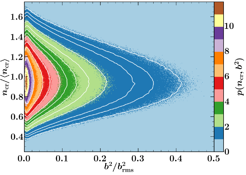
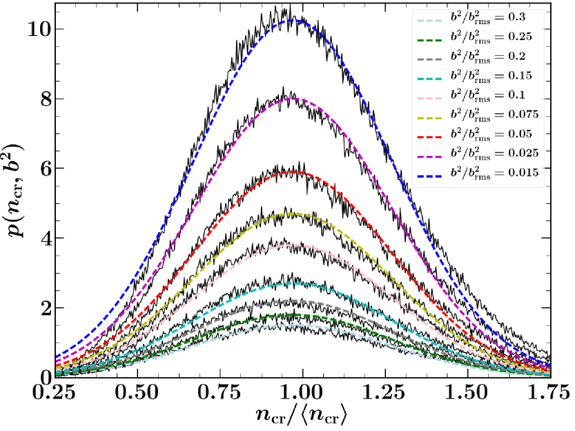
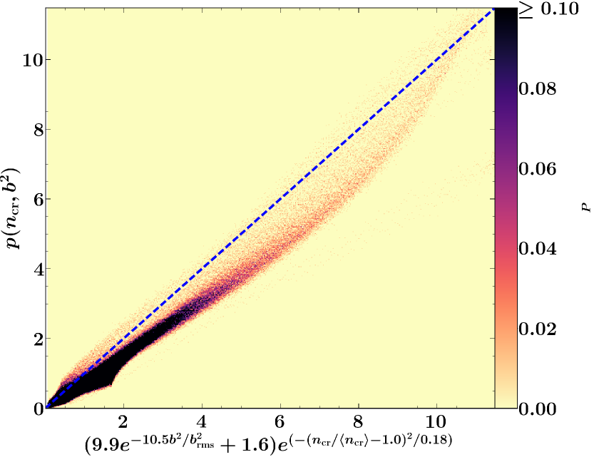
Figure 14: The joint probability density function (PDF) $p(n_{\rm cr},b^{2})$ of $b^{2}/\,b_{\rm rms}^{2}$ and $n_{\rm cr}/\langle n_{\rm cr}\rangle$ in the intermittent magnetic field for $0\leq b^{2}/\,b_{\rm rms}^{2}\leq 0.5$ and $0.25\leq n_{\rm cr}/\langle n_{\rm cr}\rangle\leq 1.75$ (upper left panel). The joint PDF $p(n_{\rm cr},b^{2})$ as a function of $n_{\rm cr}/\langle n_{\rm cr}\rangle$ alone for various fixed values of $b^{2}/\,b_{\rm rms}^{2}$ is shown in the upper right panel together with least-square fits of the form $p(n_{\rm cr},b^{2})=A(b^{2})\mathrm{e}^{-(n_{\rm cr}-1.0)^{2}/0.18}$ (smooth dashed curves). The lower left panel presents $A$ as a function of $b^{2}/\,b_{\rm rms}^{2}$ fitted with an exponential (red, dashed). The lower right panel shows the $2d$ histogram of the computed and fitted values of $p(n_{\rm cr},b^{2})$, with a linear fit (dashed, blue).

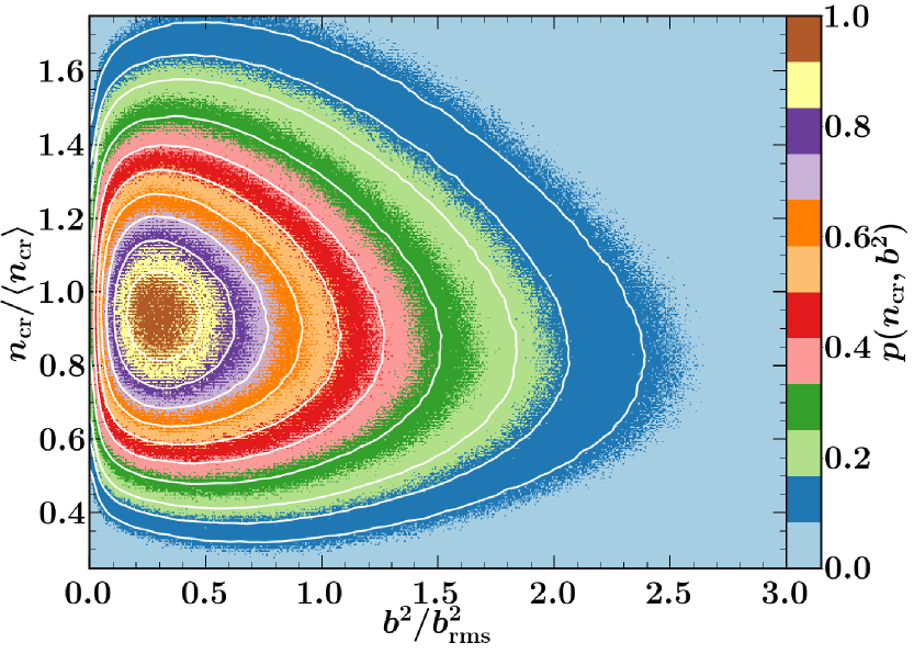
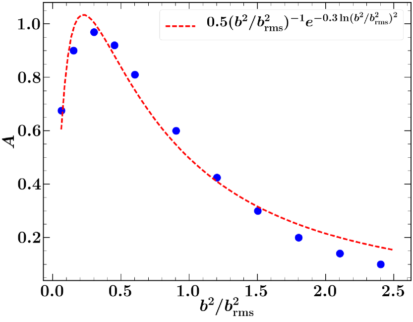
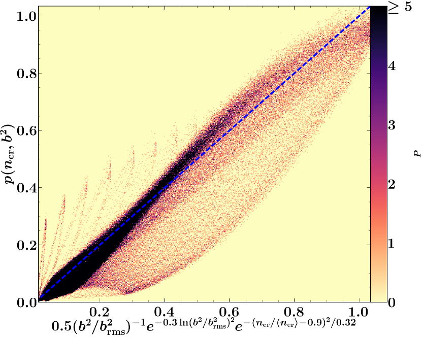
Figure 15: As in Fig. 14 but for the randomized (Gaussian) magnetic field for $0\leq b^{2}/\,b_{\rm rms}^{2}\leq 3.0$ and $0.25\leq n_{\rm cr}/\langle n_{\rm cr}\rangle\leq 1.75$ and the lower right panel shows the $2d$ histogram with blue-dashed line as $y=x$ (the bisector of the angle between the axes).

Appendix C Statistical independence of cosmic ray and magnetic field distributions

The distributions of cosmic rays and magnetic field energy density are uncorrelated (as discussed in Sec. 4.2) and we check for their statistical independence, i.e., whether $p(n_{\rm cr},b^{2})$, the joint probability distribution function of two components is equal to $p(n_{\rm cr})p(b^{2})$, the product of the probability distribution function of each component. This is tested especially for the core region where $n_{\rm cr}$ is close to its mean value. The upper left panels of Figures 14 and 15 show the joint probability densities of magnetic field strength and cosmic ray number densities in the intermittent and Gaussian (randomized) magnetic fields, respectively. We use the Kolmogorov–Smirnov (KS) test to check whether the two distributions are independent. We perform KS test on marginal probability distributions, $p(b|n_{\rm cr})$ and $p(n_{\rm cr}|b)$ to check whether each of them are drawn from the same distribution. This is measured by the $D$ statistics of the test, which is the absolute maximum distance between the cumulative distribution function of the two samples. A value of $D$ smaller than 0.087 represents $95\%$ confidence that the two samples are drawn from the same distribution. For this we consider two samples from the marginal probability distribution $p(b|n_{\rm cr})$ with consecutive $n_{\rm cr}$ (cuts along consecutive values of $y$ axis of upper left panel of Fig. 14). We performed the KS test for all such pairs and found the mean value of $D$ to be $\simeq 0.062$. A similar calculation for $p(n_{\rm cr}|b)$ gives $\simeq 0.072$. The mean $D$ values for Gaussian (randomized) magnetic fields are $\simeq 0.054$ for $p(n_{\rm cr}|b)$ and $\simeq 0.114$ for $p(b|n_{\rm cr})$ respectively. The small $D$ values suggest that the cosmic ray number density and magnetic field distributions are independent of each other and the joint probability $p(n_{\rm cr},b^{2})$ can be factorized into $p(n_{\rm cr})$ and $p(b^{2})$. We find the functional dependence of $p(n_{\rm cr})$ on $n_{\rm cr}$ and $p(b^{2})$ on $b^{2}$ as follows. Cuts through the joint PDF in the intermittent magnetic field, shown in the upper right panel of Fig. 14 are well fitted with a Gaussian which, remarkably, has neither the mean value nor the standard deviation dependent on $b$. The dependence of the maximum value of the conditional PDF $p_{n}(n_{\rm cr}|b^{2})$ on $b^{2}$ is shown in the lower left panel of Fig. 14 together with its fit with an exponential function. Thus, the joint PDF of $n_{\rm cr}$ and $b$ has the form

$$p(n_{\rm cr},b)\approx(1.6+9.9\mathrm{e}^{-10.5b^{2}/\,b_{\rm rms}^{2}})\mathrm{e}^{-(n_{\rm cr}/\langle n_{\rm cr}\rangle-1)^{2}/0.18}$$ (17)

for $0\leq b^{2}/\,b_{\rm rms}^{2}\leq 0.3$ and $0.25\leq n_{\rm cr}/\langle n_{\rm cr}\rangle\leq 1.75$. The relative accuracy of the fitted parameters is better than $5$ per cent. This is confirmed by the $2d$ histogram of the measured and fitted values of $p(n_{\rm cr},b)$ shown in the lower left panel of Fig. 14: for a perfect fit, the points would be all on the bisector of the quadrant angle. The scatter about that line, shown dashed (blue) provides a measure of the accuracy of the fit. A very small number of points systematically deviate from the main dependence, yet lying on a straight line as well. The joint PDF is thus factorizable emphasizing that both the distribution are independent.

Similar analysis for $p(n_{\rm cr},b)$ in the randomized (Gaussian) magnetic field is illustrated in Fig. 15. As in the intermittent magnetic field, the joint PDF is roughly factorizable and thus $n_{\rm cr}$ and $b$ are statistically independent. The form of the conditional PDF of magnetic field strength is a lognormal distribution,

$$p(b|n_{\rm cr})\approx 0.5(b^{2}/\,b_{\rm rms}^{2})^{-1}\mathrm{e}^{-0.3\ln(b^{2}/\,b_{\rm rms}^{2})^{2}}$$ (18)

for $0\leq b^{2}/\,b_{\rm rms}^{2}\leq 3$. We find that

$$p(n_{\rm cr},b)\approx 0.5(b^{2}/\,b_{\rm rms}^{2})^{-1}\mathrm{e}^{-0.3\ln(b^{2}/\,b_{\rm rms}^{2})^{2}}\mathrm{e}^{-(n_{\rm cr}/\langle n_{\rm cr}\rangle-0.9)^{2}/0.32}\,.$$ (19)

The $2d$ histogram of the measured and fitted values is shown (with the dashed (blue) line for the perfect match) in the lower right panel of Fig. 15.

To summarize, the distributions of cosmic ray number density and magnetic field strength are statistically independent in the diffusive regime of the cosmic rays. In the intermittent magnetic field, the joint PDF of $n_{\rm cr}$ and $b$ is well approximated by a Gaussian in $n_{\rm cr}$ and a modified Gaussian in $b$. In randomized (Gaussian) field, the joint PDF is approximated by a Gaussian in $n_{\rm cr}$ and a lognormal distribution in $b^{2}$. The two variables remain statistically independent for cosmic rays of other energies too. The exact parameters of the joint PDF are likely to depend on details of the magnetic field structure and the energy of the particle.

References

- Arbutina et al. (2012) Arbutina B., Urošević D., Andjelić M. M., Pavlović M. Z., Vukotić B., 2012, Astrophys. J., 746, 79
- Basu & Roy (2013) Basu A., Roy S., 2013, Mon. Not. R. Astron. Soc., 433, 1675
- Beck (2016) Beck R., 2016, A&ARv, 24, 4
- Beck & Krause (2005) Beck R., Krause M., 2005, Astron. Nachr., 326, 414
- Beck et al. (1996) Beck R., Brandenburg A., Moss D., Shukurov A., Sokoloff D., 1996, Ann. Rev. Astron. Astrophys., 34, 155
- Beck et al. (2003) Beck R., Shukurov A., Sokoloff D., Wielebinski R., 2003, Astron. Astrophys., 411, 99
- Berezinskii et al. (1990) Berezinskii V. S., Bulanov S. V., Dogiel V. A., Ptuskin V. S., 1990, Astrophysics of Cosmic Rays. North-Holland, Amsterdam
- Berkhuijsen et al. (2013) Berkhuijsen E. M., Beck R., Tabatabaei F. S., 2013, Mon. Not. R. Astron. Soc., 435, 1598
- Biskamp (2003) Biskamp D., 2003, Magnetohydrodynamic Turbulence. Cambridge University Press, Cambridge, UK
- Brandenburg & Subramanian (2005) Brandenburg A., Subramanian K., 2005, Phys. Rep., 417, 1
- Burbidge (1956) Burbidge G. R., 1956, Astrophys. J., 124, 416
- Bykov (1988) Bykov A. M., 1988, Sov. Astron. Lett., 14, 60
- Bykov & Toptygin (1985) Bykov A. M., Toptygin I. N., 1985, Sov. Astron. Lett., 11, 75
- Bykov & Toptygin (1987) Bykov A. M., Toptygin I. N., 1987, Astrophys. Space Sci., 138, 341
- Candia & Roulet (2004) Candia J., Roulet E., 2004, J. Cosmol. Astropart. Phys., 10, 7
- Casse et al. (2002) Casse F., Lemoine M., Pelletier G., 2002, Phys. Rev. D, 65, 023002
- Cesarsky & Kulsrud (1981) Cesarsky C. J., Kulsrud R. M., 1981, in Setti G., Spada G., Wolfendale A. W., eds, IAU Symposium Vol. 94, Origin of Cosmic Rays. p. 251
- Chamandy et al. (2014) Chamandy L., Shukurov A., Subramanian K., Stoker K., 2014, Mon. Not. R. Astron. Soc., 443, 1867
- Chandran (2000) Chandran B. D. G., 2000, Astrophys. J., 529, 513
- DeMarco et al. (2007) DeMarco D., Blasi P., Stanev T., 2007, J. Cosmol. Astropart. Phys., 6, 027
- Desiati & Zweibel (2014) Desiati P., Zweibel E. G., 2014, Astrophys. J., 791, 51
- Evirgen et al. (2017) Evirgen C. C., Gent F. A., Shukurov A., Fletcher A., Bushby P., 2017, Mon. Not. R. Astron. Soc., 464, L105
- Farmer & Goldreich (2004) Farmer A. J., Goldreich P., 2004, Astrophys. J., 604, 671
- Federrath et al. (2010) Federrath C., Roman-Duval J., Klessen R. S., Schmidt W., Mac Low M.-M., 2010, Astron. Astrophys., 512, A81
- Felice & Kulsrud (2001) Felice G. M., Kulsrud R. M., 2001, Astrophys. J., 553, 198
- Fung et al. (1992) Fung J. C. H., Hunt J. C. R., Malik N. A., Perkins R. J., 1992, J. Fluid Mech., 236, 281
- Gaensler et al. (2011) Gaensler B. M., et al., 2011, Nature, 478, 214
- Giacalone & Jokipii (1999) Giacalone J., Jokipii J. R., 1999, Astrophys. J., 520, 204
- Globus et al. (2008) Globus N., Allard D., Parizot E., 2008, Astron. Astrophys., 479, 97
- Grenier et al. (2015) Grenier I. A., Black J. H., Strong A. W., 2015, Ann. Rev. Astron. Astrophys., 53, 199
- Harari et al. (2014) Harari D., Mollerach S., Roulet E., 2014, Phys. Rev. D, 89, 123001
- Haverkorn & Spangler (2013) Haverkorn M., Spangler S. R., 2013, SSRv, 178, 483
- Heiles & Troland (2005) Heiles C., Troland T. H., 2005, Astrophys. J., 624, 773
- Hoernes et al. (1998) Hoernes P., Berkhuijsen E. M., Xu C., 1998, Astron. Astrophys., 334, 57
- Jackson (1998) Jackson J. D., 1998, Classical Electrodynamics, 3rd Edition. Wiley, New York
- Kalberla & Kerp (2016) Kalberla P. M. W., Kerp J., 2016, Astron. Astrophys., 595, A37
- Kazantsev (1967) Kazantsev A. P., 1967, Zh. Eksper. Teor. Fiz., 53, 1807
- Klein & Fletcher (2015) Klein U., Fletcher A., 2015, Galactic and Intergalactic Magnetic Fields. Springer Praxis Books, Springer International Publishing, Heidelberg, Germany
- Kulsrud (2005) Kulsrud R. M., 2005, Plasma Physics for Astrophysics. Princeton University Press, Princeton
- Kulsrud & Pearce (1969) Kulsrud R., Pearce W. P., 1969, Astrophys. J., 156, 445
- Michalek & Ostrowski (1997) Michalek G., Ostrowski M., 1997, Astron. Astrophys., 326, 793
- Moffatt (1978) Moffatt H. K., 1978, Magnetic field generation in electrically conducting fluids.. Cambridge University Press, Cambridge
- Monin & Yaglom (1971) Monin A. S., Yaglom A. M., 1971, Statistical Fluid Mechanics. MIT Press, Cambridge, Massachusetts, USA
- Moss et al. (2007) Moss D., Snodin A. P., Englmaier P., Shukurov A., Beck R., Sokoloff D. D., 2007, Astron. Astrophys., 465, 157
- Parizot (2004) Parizot E., 2004, Nucl. Phys. B, Proc. Suppl., 136, 169
- Plotnikov et al. (2011) Plotnikov I., Pelletier G., Lemoine M., 2011, Astron. Astrophys., 532, A68
- Ruzmaikin et al. (1989) Ruzmaikin A., Sokoloff D., Shukurov A., 1989, Mon. Not. R. Astron. Soc., 241, 1
- Schekochihin et al. (2004) Schekochihin A. A., Cowley S. C., Taylor S. F., Maron J. L., McWilliams J. C., 2004, Astrophys. J., 612, 276
- Schekochihin et al. (2009) Schekochihin A. A., Cowley S. C., Dorland W., Hammett G. W., Howes G. G., Quataert E., Tatsuno T., 2009, ApJS, 182, 310
- Schlickeiser (2002) Schlickeiser R., 2002, Cosmic Ray Astrophysics. Springer, Berlin
- Shalchi (2009) Shalchi A., 2009, Nonlinear Cosmic Ray Diffusion Theories. Vol. 362, Springer, Berlin
- Shukurov et al. (2017) Shukurov A., Snodin A. P., Seta A., Bushby P. J., Wood T. S., 2017, Astrophys. J. Lett., 839, L16
- Snodin et al. (2006) Snodin A. P., Brandenburg A., Mee A. J., Shukurov A., 2006, Mon. Not. R. Astron. Soc., 373, 643
- Snodin et al. (2013) Snodin A. P., Ruffolo D., Oughton S., Servidio S., Matthaeus W. H., 2013, Astrophys. J., 779, 56
- Snodin et al. (2016) Snodin A. P., Shukurov A., Sarson G. R., Bushby P. J., Rodrigues L. F. S., 2016, Mon. Not. R. Astron. Soc., 457, 3975
- Stepanov et al. (2014) Stepanov R., Shukurov A., Fletcher A., Beck R., La Porta L., Tabatabaei F., 2014, Mon. Not. R. Astron. Soc., 437, 2201
- Strong et al. (2007) Strong A. W., Moskalenko I. V., Ptuskin V. S., 2007, Annual Review of Nuclear and Particle Science, 57, 285
- Subedi et al. (2017) Subedi P., et al., 2017, Astrophys. J., 837, 140
- Subramanian (1999) Subramanian K., 1999, Phys. Rev. Lett., 83, 2957
- Subramanian et al. (2006) Subramanian K., Shukurov A., Haugen N. E. L., 2006, Mon. Not. R. Astron. Soc., 366, 1437
- Wentzel (1974) Wentzel D. G., 1974, Ann. Rev. Astron. Astrophys., 12, 71
- Wilkin et al. (2007) Wilkin S. L., Barenghi C. F., Shukurov A., 2007, Phys. Rev. Lett., 99, 134501
- Zaroubi et al. (2015) Zaroubi S., et al., 2015, Mon. Not. R. Astron. Soc., 454, L46
- Zeldovich et al. (1990) Zeldovich Ya. B., Ruzmaikin A. A., Sokoloff D. D., 1990, The Almighty Chance. World Scientific, Singapore
- Zelenyi et al. (2015) Zelenyi L. M., Bykov A. M., Uvarov Y. A., Artemyev A. V., 2015, J. Plasma. Phys., 81, 395810401