The Importance of Urca-process Cooling in Accreting ONe White Dwarfs

Abstract

We study the evolution of accreting oxygen-neon (ONe) white dwarfs (WDs), with a particular emphasis on the effects of the presence of the carbon-burning products $\mathrm{{}^{23}Na}$ and $\mathrm{{}^{25}Mg}$. These isotopes lead to substantial cooling of the WD via the $\mathrm{{}^{25}Mg}$-$\mathrm{{}^{25}Na}$, $\mathrm{{}^{23}Na}$-$\mathrm{{}^{23}Ne}$, and $\mathrm{{}^{25}Na}$-$\mathrm{{}^{25}Ne}$ Urca pairs. We derive an analytic formula for the peak Urca-process cooling rate and use it to obtain a simple expression for the temperature to which the Urca process cools the WD. Our estimates are equally applicable to accreting carbon-oxygen WDs. We use the Modules for Experiments in Stellar Astrophysics (MESA) stellar evolution code to evolve a suite of models that confirm these analytic results and demonstrate that Urca-process cooling substantially modifies the thermal evolution of accreting ONe WDs. Most importantly, we show that MESA models with lower temperatures at the onset of the $\mathrm{{}^{24}Mg}$ and $\mathrm{{}^{24}Na}$ electron captures develop convectively unstable regions, even when using the Ledoux criterion. We discuss the difficulties that we encounter in modeling these convective regions and outline the potential effects of this convection on the subsequent WD evolution. For models in which we do not allow convection to operate, we find that oxygen ignites around a density of $\log(\rho_{\mathrm{c}}/\mathrm{g\,cm^{-3}})\approx 9.95$, very similar to the value without Urca cooling. Nonetheless, the inclusion of the effects of Urca-process cooling is an important step in producing progenitor models with more realistic temperature and composition profiles which are needed for the evolution of the subsequent oxygen deflagration and hence for studies of the signature of accretion-induced collapse.

1 Introduction

In the Urca process, first discussed by Gamow & Schoenberg (1941), repeated electron-capture and beta-decay reactions give rise to neutrino emission. When this occurs in a stellar interior where the neutrinos are able to free-stream out of the star—such as in a white dwarf (WD)—it becomes an active cooling process. Tsuruta & Cameron (1970) calculated analytic approximations to the energy loss rates from the Urca process and compiled a list of 132 pairs of isotopes that contribute to these energy losses. Paczyński (1973) applied these results in a study of the temperature evolution of degenerate carbon-oxygen (CO) cores, demonstrating that this cooling can shift the density at which pycnonuclear carbon ignition occurs.

In Paczyński (1973) the odd mass number nuclei that participate in the Urca process were assumed to have cosmic abundances. Carbon burning, however, produces significant mass fractions of $\mathrm{{}^{23}Na}$ and $\mathrm{{}^{25}Mg}$. Therefore Urca-process cooling will be significantly more important in stars with oxygen-neon (ONe) compositions, where the material has already been processed by carbon burning (Iben, 1978), such as in the cores of super-asymptotic giant branch stars (Toki et al., 2013; Jones et al., 2013).

In Schwab et al. (2015), hereafter referred to as SQB15, we developed an analytic and numerical understanding of the evolution of ONe WDs towards accretion-induced collapse (AIC) in which we considered only $\mathrm{{}^{24}Mg}$, $\mathrm{{}^{20}Ne}$, and $\mathrm{{}^{16}O}$. In this work, we extend and modify this understanding to include additional odd mass number isotopes generated during carbon-burning, namely $\mathrm{{}^{23}Na}$ and $\mathrm{{}^{25}Mg}$. We demonstrate analytically and numerically that significant temperature changes occur due to Urca-process cooling and we illustrate its effect on the subsequent evolution. Most importantly, we find that the Urca process alters the temperature profile of the WD in such a way that regions of the WD become convectively unstable after the electron captures on $\mathrm{{}^{24}Mg}$ occur.

In Section 2, we provide an overview of the microphysics of the Urca process and identify the important isotopes and their threshold densities. In Section 3, we make analytic estimates of the importance of Urca-process cooling in accreting ONe WDs. In Section 4, we discuss how we use the MESA stellar evolution code to demonstrate the effects of Urca-process cooling. In Section 5, we discuss and characterize the effects of incomplete nuclear data. In Section 6, we demonstrate and explain the onset of convective instability in our MESA models. In Section 7, we discuss the evolution of the WD up to oxygen ignition. In Section 9, we conclude.

2 The Urca Process

Take two nuclei $a\equiv(Z,A)$ and $b\equiv(Z-1,A)$ that are connected by an electron-capture transition

$$(Z,A)+e^{-}\to(Z-1,A)+\nu_{e}$$ (1)

and beta-decay transition

$$(Z-1,A)\to(Z,A)+e^{-}+\bar{\nu}_{e}$$ (2)

where $Z$ and $A$ are respectively the atomic number and mass number of the nucleus. In all of the electron-capture transitions considered here, there is a threshold energy required for the electron. In a cold, degenerate plasma, electrons with sufficient energy will become available when the Fermi energy $E_{\mathrm{F}}$ is equal to the energy difference between the parent and daughter states $Q_{0}$, which includes both the nuclear rest mass and the energy associated with excited states. In the limit of relativistic electrons, this corresponds to a threshold density

$$\rho_{0}\approx 1.8\times 10^{9}\,\mathrm{\mathrm{g\,cm^{-3}}}\,\left(\frac{Y_{\mathrm{e}}}{0.5}\right)^{-1}\left(\frac{|Q_{0}|}{5\,\mathrm{MeV}}\right)^{3}~{}.$$ (3)

where $Y_{\mathrm{e}}$ is the electron fraction.

2.1 Cooling Rate

At the threshold density the rates of electron capture and beta decay are comparable. Since each reaction produces a neutrino that free-streams out of the star, this is a cooling process.

Suppose the total number density of the two isotopes in the Urca pair is $n_{u}=n_{a}+n_{b}$. Because the time-scales for electron capture and beta decay are short compared to the evolutionary time-scale of the system, an equilibrium is achieved. The relative abundances are then given by the detailed balance condition $n_{a}\lambda_{\mathrm{ec}}+n_{b}\lambda_{\beta}=0$. Under this assumption, the specific neutrino cooling rate from the Urca process can be written as

$$\epsilon_{\mathrm{u}}=\frac{n_{u}}{\rho}C=\frac{X_{u}}{A_{u}m_{\mathrm{u}}}C$$ (4)

where $X_{u}$ is the mass fraction of the Urca pair, $A_{u}$ is its atomic mass number, $m_{\mathrm{u}}$ is the atomic mass unit, and

$$C=\frac{\varepsilon_{\nu,\mathrm{ec}}\lambda_{\beta}+\varepsilon_{\nu,\beta}\lambda_{\mathrm{ec}}}{\lambda_{\beta}+\lambda_{\mathrm{ec}}}~{}.$$ (5)

In Appendix A, we write out the full expressions for the rates ($\lambda$) and neutrino loss rates ($\varepsilon_{\nu}$) for electron capture and beta decay necessary to evaluate equation (5). The key result is that the Urca-process cooling rate for an allowed ground state to ground state transition is sharply peaked at $E_{\mathrm{F}}=|Q_{\mathrm{g}}|$ and that the maximum value of $C$ is

$$C_{\mathrm{max}}=\frac{7\pi^{4}\ln 2}{60}\frac{m_{\mathrm{e}}c^{2}}{(ft)_{\beta}+(ft)_{\mathrm{ec}}}\left(\frac{k_{\mathrm{B}}T}{m_{\mathrm{e}}c^{2}}\right)^{4}\left(\frac{Q_{\mathrm{g}}}{m_{\mathrm{e}}c^{2}}\right)^{2}\exp({\pi\alpha Z})~{},$$ (6)

where $ft$ is the comparative half-life, $\alpha$ is the fine structure constant, and $Q_{\mathrm{g}}$ is the threshold energy for the ground state to ground state transition.

2.2 Isotopes and Transitions

Table 1: A summary of the key weak reactions that occur in accreting ONe WDs. Only the lowest energy allowed transition from the ground state is listed, since this typically sets the threshold density; this is not an exhaustive list of the transitions considered in this work. Electron captures convert the initial isotope to the final isotope. $Q_{\mathrm{g}}$ is the rest mass difference between the ground states of the isotopes (in $\mathrm{MeV}$); unlike in the similar tabulation in SQB15 we have already accounted for the electron rest mass. $E_{\mathrm{i}}$ and $E_{\mathrm{f}}$ are the excitation energies of the initial and final states, relative to the ground state (in $\mathrm{MeV}$). $J_{\mathrm{i}}^{\pi}$ and $J_{\mathrm{f}}^{\pi}$ are the spins and parities of the initial and final states. $ft$ is the comparative half-life (in $\mathrm{s}$) for this transition. $Q_{0}$ is the threshold energy difference (in $\mathrm{MeV}$); this includes the energy associated with excited states. $\rho_{0}$ is the approximate density (in $\mathrm{g\,cm^{-3}}$) at which the reaction occurs (as defined in equation 3). Effect indicates whether the net effect of the weak reactions is to cool the plasma via Urca-process cooling (odd mass number) or heat the plasma via exothermic electron captures (even mass number). The nuclear data is drawn from the literature (Tilley et al., 1998; Firestone, 2007a, b, 2009; Martínez-Pinedo et al., 2014).

Initial	Final	$Q_{\mathrm{g}}$	$E_{\mathrm{i}}$	$J_{\mathrm{i}}^{\pi}$	$E_{\mathrm{f}}$	$J_{\mathrm{f}}^{\pi}$	$\log(ft)$	$Q_{0}$	$\log\rho_{0}$	Effect	Notes
$\mathrm{{}^{25}Mg}$	$\mathrm{{}^{25}Na}$	-4.346	0.000	$5/2^{+}$	0.000	$5/2^{+}$	5.26	-4.346	9.07	Cool
$\mathrm{{}^{23}Na}$	$\mathrm{{}^{23}Ne}$	-4.887	0.000	$3/2^{+}$	0.000	$5/2^{+}$	5.27	-4.887	9.22	Cool
$\mathrm{{}^{24}Mg}$	$\mathrm{{}^{24}Na}$	-6.026	0.000	$0^{+}$	0.472	$1^{+}$	4.82	-6.498	9.60	Heat
$\mathrm{{}^{24}Na}$	$\mathrm{{}^{24}Ne}$	-2.978	0.000	$4^{+}$	3.972	$4^{+}$	6.21	-6.950	9.69	Heat	a
$\mathrm{{}^{25}Na}$	$\mathrm{{}^{25}Ne}$	-7.761	0.090	$3/2^{+}$	0.000	$1/2^{+}$	4.41	-7.671	9.81	Cool	b
$\mathrm{{}^{20}Ne}$	$\mathrm{{}^{20}F}$	-7.536	0.000	$0^{+}$	1.057	$1^{+}$	4.38	-8.593	9.96	Heat	a,c
$\mathrm{{}^{23}Ne}$	$\mathrm{{}^{23}F}$	-8.991	0.000	$5/2^{+}$	0.000	$5/2^{+}$	5.72	-8.991	10.02	Cool	d
a this reaction is affected by a nonunique second forbidden transition; see Section 5
b the ground state has $J^{\pi}=5/2^{+}$; for the relevant temperatures this low-lying excited state is populated
c the $\mathrm{{}^{20}F}$ will immediately undergo an electron capture to form $\mathrm{{}^{20}O}$
d the oxygen deflagration begins before our models reach this density

Using a nuclear reaction network with 244 species and analytic weak reaction rates, Iben (1978) identified Urca pairs for which the neutrino loss rates rival or exceed thermal neutrino losses. In material processed by carbon burning, the two most abundant odd mass number isotopes are $\mathrm{{}^{23}Na}$ and $\mathrm{{}^{25}Mg}$ and thus the most important Urca pairs have $A=23$ and $25$ (see figure 2 in Iben, 1978). Therefore, we restrict our attention to these isotopes, neglecting possible small contributions from $A=21$ and $29$ isotopes.

The nuclear data (energy levels and $ft$ values) required for this calculation are drawn from the literature (Tilley et al., 1998; Firestone, 2007a, b, 2009; Martínez-Pinedo et al., 2014). Table 1 summarizes this data. Fig. 1 shows a simplified level structure (excluding excited states $\ga 1\,\mathrm{MeV}$ above the ground state) of the $A=23$ and $A=25$ nuclei that we consider. In Section 5, we will discuss the $A=20$ and $A=24$ nuclei in more detail.

Figure 1: Energy level diagrams for the $A=25$ (left) and $A=23$ (right) nuclei that we consider. The $J^{\pi}$ value is indicated at the right of each level and is sometimes given an arbitrary offset (indicated via a thin line) in order to enhance legibility. The most important transitions we consider are indicated with arrows. The transition between $\mathrm{{}^{25}Ne}$ and $\mathrm{{}^{25}Na}$ is to/from the low-lying first excited state of $\mathrm{{}^{25}Na}$.

While this work was in preparation, new weak reaction rate tables for A=17-28 nuclei were published by Suzuki et al. (2016). In Appendix D we compare our fiducial model with a MESA calculation using those tables. We find good agreement.

3 Analytic Estimates

The energy equation for material in a spherically symmetric star is

$$T\frac{ds}{dt}=\epsilon-\frac{\partial L}{\partial M}$$ (7)

where $\epsilon$ is the specific energy generation rate, which includes nuclear reactions, neutrino processes, etc. For these estimates, we will consider only the effects of neutrino losses, which we sub-divide into $\epsilon_{\nu}$ (thermal neutrino loss rate) and $\epsilon_{\mathrm{u}}$ (Urca process neutrino loss rate). In the centre of these rapidly accreting WDs, $\partial L/\partial M$ is negligible, and therefore

$$-\left(\epsilon_{\nu}+\epsilon_{\mathrm{u}}\right)=T_{\mathrm{\!c}}\ c_{\mathrm{v}}\left[\frac{d\ln T_{\mathrm{\!c}}}{dt}-(\Gamma_{3}-1)\frac{d\ln\rho_{\mathrm{c}}}{dt}\right]~{},$$ (8)

where $c_{\mathrm{v}}$ is the specific heat at constant volume and $\Gamma_{3}-1=\left(d\ln T/d\ln\rho\right)_{\mathrm{ad}}$. Depending on which terms dominate, there are three regimes for the evolution of the central temperature:

1. When the left hand side of equation (8) is negligible, the central temperature will evolve along an adiabat.

2. When $\epsilon_{\nu}$ dominates the left hand side of equation (8), the temperature will evolve towards (and then along) the attractor solution discussed by Paczyński (1973), SQB15, and Brooks et al. (2016), in which thermal neutrino cooling and compressional heating balance. Because of the neutrino losses, this attractor solution is shallower (in $T$-$\rho$ space) than an adiabat, though it still has positive slope.

3. When $\epsilon_{u}$ dominates the left hand side of equation (8), the temperature will decrease. Because the Urca-process cooling is sharply peaked in $E_{\mathrm{F}}$, this will occur at nearly fixed density.

These three regimes are illustrated in Fig. 2, which shows the evolution of the central density and temperature in one of our MESA models, centered on the density where cooling due to the $\mathrm{{}^{23}Na}$-$\mathrm{{}^{23}Ne}$ Urca pair occurs.

Figure 2: The schematic evolution of central density and temperature in a ONe WD accreting at $10^{-6}\rm\mathrm{M}_{\sun}\,yr^{-1}$. The black line shows the result of evolving a MESA model that has an initial mass fraction of 0.01 $\mathrm{{}^{23}Na}$. The three regimes discussed in Section 3 are labeled.

It is useful to estimate the magnitude of the temperature decrease caused by the Urca process (regime iii). As we will show, this depends primarily on the mass fraction of the Urca pair and the rate at which the core is being compressed. Paczyński (1973) provides a fitting formula for the temperature change, obtained though careful numerical integration; however this result is unsuitable for our purposes, as it assumes that the value of $d\ln\rho/dt$ is that of a CO core growing via stable He-shell burning, as set by the core mass-luminosity relation.

We assess the Urca-process cooling via a simpler argument. As a result of accretion, the core is being compressed on a time-scale

$$t_{\rho}=\left(\frac{d\ln\rho_{c}}{dt}\right)^{-1}=\left(\frac{d\ln\rho_{c}}{d\ln M}\right)^{-1}\frac{M}{\dot{M}}~{}~{}~{}.$$ (9)

For an ideal, zero-temperature white dwarf, in the range $9\la\log(\rho_{\mathrm{c}}/\mathrm{g\,cm^{-3}})\la 10$ and with $Y_{\mathrm{e}}\approx 0.5$, SQB15 give the approximate result that

$$t_{\rho}\approx 5\times 10^{4}\,\mathrm{yr}\,\rho_{9}^{-0.55}\dot{M}_{-6}^{-1}$$ (10)

where $\rho_{9}=\rho/(10^{9}\,\mathrm{g~{}cm^{-3}})$ and $\dot{M}_{-6}=\dot{M}/({10^{-6}\,\mathrm{\rm\mathrm{M}_{\sun}\,yr^{-1}}})$.

The cooling from an individual Urca pair peaks when $E_{\mathrm{F}}=Q_{\mathrm{g}}$, and is significant for only $\Delta E_{\mathrm{F}}\approx 3k_{\mathrm{B}}T$ centered around this peak (see Appendix A, in particular equation 36). We can estimate the width of the peak (in density) as $\Delta\ln\rho\approx 3\Delta E_{\mathrm{F}}/E_{\mathrm{F}}$. Therefore, the time-scale for a parcel to cross the cooling region is

$$t_{\textrm{cross}}\approx\left(\frac{9k_{\mathrm{B}}T}{E_{\mathrm{F}}}\right)t_{\rho} \approx 2\times 10^{-2}\,T_{8}\rho_{9}^{-1/3}t_{\rho}$$ (11)

$$\approx 1\times 10^{3}\,\mathrm{yr}\,T_{8}\rho_{9}^{-0.88}\dot{M}_{-6}^{-1}~{}.$$ (12)

At the density where the Urca-process cooling peaks, the cooling time-scale $t_{\textrm{cool}}$ is

$$t_{\textrm{cool}}=\frac{c_{\mathrm{v}}T}{\epsilon_{\mathrm{max}}}=\frac{3k_{\mathrm{B}}TA_{\mathrm{u}}}{\bar{A}X_{\mathrm{u}}C_{\mathrm{max}}}$$ (13)

where we have taken $\epsilon_{\mathrm{max}}$ from the combination of equations (4) and (6), and we have assumed the specific heat is that given by the Dulong-Petit law ($c_{\mathrm{v}}=3k_{\mathrm{B}}/\bar{A}$). Assuming $A_{\mathrm{u}}\approx\bar{A}$,

$$t_{\textrm{cool}}\approx 4\times 10^{2}\,\mathrm{yr}\,T_{8}^{-3}\left(\frac{X_{\mathrm{u}}}{0.01}\right)^{-1}\left(\frac{Q_{\mathrm{g}}}{5\,\mathrm{MeV}}\right)^{-2}\left(\frac{ft}{10^{5}\,\mathrm{s}}\right)~{}.$$ (14)

When the core reaches a density where Urca-process cooling will begin, its initial temperature will have been set by its evolution in regimes (i) or (ii). If $t_{\textrm{cross}}>t_{\textrm{cool}}$ initially, since $t_{\textrm{cool}}$ increases more rapidly with decreasing temperature than $t_{\textrm{cross}}$, the core will evolve towards the condition $t_{\textrm{cross}}\approx t_{\textrm{cool}}$. When this condition is reached, the Urca-process cooling will effectively shut off, since the core will evolve out of the cooling region before significant additional cooling occurs. If $t_{\textrm{cross}}<t_{\textrm{cool}}$ initially—which is never true in the cases we consider—then significant Urca-process cooling will not occur.

Therefore, the relation $t_{\textrm{cross}}\approx t_{\textrm{cool}}$ gives us an estimate for the temperature to which each Urca pair will cool the star. Combining equations (11) and (13) and taking the fiducial values $Q_{\mathrm{g}}=5\,\mathrm{MeV}$, $ft=10^{5}\,\mathrm{s}$, and using a density equal to the threshold density (equation 3) for this $Q_{\mathrm{g}}$, we find that the temperature to which the core cools is

$$T_{\mathrm{u}}\approx 9\times 10^{7}\,\mathrm{K}\,\dot{M}_{-6}^{1/4}\left(\frac{X_{\mathrm{u}}}{0.01}\right)^{-1/4}~{}.$$ (15)

In order to validate this relation we ran a suite of MESA models varying $X_{\mathrm{u}}$ and $\dot{M}$. These numerical results are shown in Figs. 3 and 4 and are in excellent agreement with the analytic scaling given in equation (15). We will discuss the implications of this cooling on the subsequent evolution in Section 6.

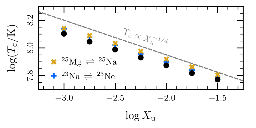
Figure 3: The minimum central temperature ($T_{\mathrm{\!c}}$) reached after Urca-process cooling as a function of the mass fraction in the Urca pair ($X_{\mathrm{u}}$). The crosses (Xs) show models with an initial mass fraction $X_{\mathrm{u}}$ of $\mathrm{{}^{23}Na}$ ($\mathrm{{}^{25}Mg}$). The solid black circles show models with initial mass fractions $X_{\mathrm{u}}$ of both $\mathrm{{}^{23}Na}$ and $\mathrm{{}^{25}Mg}$. The dashed line shows the analytically expected scaling of equation (15).

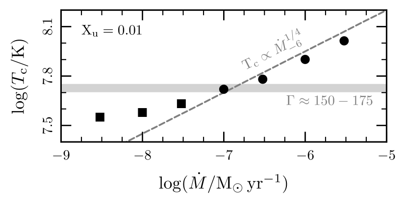
Figure 4: The minimum central temperature ($T_{\mathrm{\!c}}$) reached after Urca cooling as a function of the accretion rate ($\dot{M}$). All models have $X_{\mathrm{u}}=0.01$ as $\mathrm{{}^{23}Na}$. The solid grey band shows range of $\Gamma$ over which the latent heat of crystallization in released in MESA. Models that fully crystallized are marked with squares. The dashed line shows the analytically expected scaling of equation (15).

We note that the Urca-process cooling can be significant enough to cause the white dwarf to begin to crystallize. At densities near the $\mathrm{{}^{23}Na}$ threshold density, the condition for this phase transition $(\Gamma\approx 175)$ occurs at $T\approx 5\times 10^{7}\,\mathrm{K}$. Therefore, we expect crystallization to begin when $\dot{M}_{-6}X_{\mathrm{u}}^{-1}\la\,10$, at which point the Urca-process cooling will begin extracting the latent heat associated with the phase transition. As shown in Fig. 4, some of our models reach this regime. However, we choose not to explore the interaction of crystallization and these weak reactions further. Subsequent adiabatic compression and exothermic electron captures will cause the WD to be in the liquid state at the later times of primary interest.

4 Details of MESA Calculations

The calculations performed in this paper use MESA version 9793 (released 2017-05-31). As required by the MESA manifesto, the inlists necessary to reproduce our calculations will be posted on http://mesastar.org.

4.1 Initial Models

We generate our initial models in the same manner as SQB15, except that we stop relaxing the models at lower density ($\log(\rho_{\mathrm{c}}/\mathrm{g\,cm^{-3}})=8.6$) so that the Urca processes of interest have not yet occurred.

Our models are initially chemically homogeneous. The models shown as part of the scaling studies in Section 3 all have the indicated abundances of $\mathrm{{}^{23}Na}$ and $\mathrm{{}^{25}Mg}$, a mass fraction of 0.5 $\mathrm{{}^{16}O}$, with the remainder as $\mathrm{{}^{20}Ne}$. In Section 7, we show results from four compositions, identified as follows: SQB15, the composition used in SQB15; this paper, a similar composition plus representative mass fractions of $\mathrm{{}^{23}Na}$ and $\mathrm{{}^{25}Mg}$; T13, a composition based on the intermediate-mass star models of Takahashi et al. (2013); and F15, a composition based on the intermediate-mass star models of Farmer et al. (2015). The mass fractions of the isotopes present in each named model are shown in Table 2.

Table 2: The set of compositions used in our MESA models. Each composition is referenced in the text by the identifier listed in the top row. Each column lists the mass fractions of the isotopes (listed at left) that were included. Dashes indicate that a particular isotope was not included. The compositions T13 and F15 are based on the intermediate-mass star models of Takahashi et al. (2013) and Farmer et al. (2015) respectively.

Isotope	SQB15	This Paper	T13	F15
$\mathrm{{}^{16}O}$	0.500	0.500	0.480	0.490
$\mathrm{{}^{20}Ne}$	0.450	0.390	0.420	0.400
$\mathrm{{}^{22}Ne}$	—	—	—	0.018
$\mathrm{{}^{23}Na}$	—	0.050	0.035	0.060
$\mathrm{{}^{24}Mg}$	0.050	0.050	0.050	0.030
$\mathrm{{}^{25}Mg}$	—	0.010	0.015	0.002

4.2 Important MESA Options

While our full inlists will be made publicly available, we highlight some of the most important MESA options used in the calculations. This section assumes the reader is familiar with specific MESA options. Please consult the instrument papers (Paxton et al., 2011; Paxton et al., 2013, 2015) and the MESA website for a full explanation of the meaning of these options.

Most importantly, we use the capability of MESA to calculate weak rates from input nuclear data developed in SQB15 and validated in Paxton et al. (2015, 2016). The dangers of using coarse tabulations of the relevant weak reaction rates has been emphasized by Toki et al. (2013); this choice circumvents these issues. We activate these capabilities using the options:

    use_special_weak_rates = .true.
    ion_coulomb_corrections = ’PCR2009’
    electron_coulomb_corrections = ’Itoh2002’

Table 1 summarizes the weak reactions that we include using this capability. The files containing the input nuclear data will be made available along with our inlists.

The MESA equation of state (Paxton et al., 2011, figure 1) contains a transition from HELM (Timmes & Swesty, 2000) to PC (Potekhin & Chabrier, 2010). We set the location of this blend via the options

  log_Gamma_all_HELM = 0.60206d0 ! Gamma = 4
  log_Gamma_all_PC = 0.90309d0 ! Gamma = 8

which ensures that the core of the WD is always treated using the PC equation of state. Rapid and significant composition changes will occur as the weak equilibrium shifts. Therefore, it is necessary to ensure that all isotopes are included in the PC calculation by using the options:

    set_eos_PC_parameters = .true.
    mass_fraction_limit_for_PC = 0d0

It is essential that we choose a temporal and spatial resolution that will resolve the effects of Urca-process cooling and the exothermic electron captures. We discuss the the details of our approach in Appendix B and demonstrate that it leads to a converged result.

The choice of convective criterion is important. We use the Ledoux criterion, which accounts for the effect of composition gradients on the buoyancy. The exothermic electron captures create temperature gradients that would be unstable by the Schwarzschild criterion, but are stabilized by the $Y_{\mathrm{e}}$ gradients (Miyaji & Nomoto, 1987). Convectively stable regions with such gradients are subject to doubly-diffusive instabilities, but following the arguments in SQB15 that suggest these regions will not have time to mix, we neglect the effects of semiconvection. These choices correspond to the MESA options:

    use_Ledoux_criterion = .true.
    alpha_semiconvection = 0.0

In Section 6 we will demonstrate that convective instability can set in even when using the Ledoux criterion. Modeling this phase with standard MLT in MESA proves problematic and therefore most of the models shown use mlt_option = ’none’. This choice means that convectively unstable regions have the radiative temperature gradient and do not experience any convective mixing. A few of our models use a milder restriction, preventing convection from modifying the temperature gradient, but allowing for convective mixing. This is achieved using the control mlt_gradT_fraction = 0.

4.3 Schematic comparison with SQB15

A significant portion of the remainder of this paper will involve a discussion of the possible effects of experimentally-uncertain nonunique second forbidden transitions (Section 5) and the discovery and characterization of convective instability triggered by thermal conduction (Section 6). Before discussing these issues, it is useful to first show a model that encapsulates the effects of the $A=23$ and $A=25$ isotopes.

Fig. 5 compares the evolution of a model with the composition used in SQB15 with a model using a similar composition but including representative mass fractions of $\mathrm{{}^{23}Na}$ and $\mathrm{{}^{25}Mg}$. (The precise compositions are given in Table 2.) The models are accreting at a rate of $10^{-6}\,\mathrm{\rm\mathrm{M}_{\sun}\,yr^{-1}}$. Unless otherwise noted, all models shown use this fiducial accretion rate. The model shown in in Fig. 5 neglects forbidden transitions and assumes convective stability and thus is not the model with the “best physics”. However, it ably illustrates the main point: the evolution of the central temperature is notably different with Urca-process cooling included.

In SQB15, the temperature immediately prior to electron captures on $\mathrm{{}^{24}Mg}$ and $\mathrm{{}^{20}Ne}$ was was set by a balance between compression and neutrino cooling (the attractor solution). However, the results in Section 3 demonstrate that for a wide range of $X_{\mathrm{u}}$ and $\dot{M}$, significant Urca-process cooling will occur. In almost all cases, the WD is cooled to temperatures such that energy losses by non-nuclear neutrinos (in these conditions primarily plasma neutrinos, e.g. Itoh et al., 1996) become negligible. Therefore, we enter regime (i), and expect the material to evolve along a strongly coupled liquid adiabat. In these conditions $\Gamma_{3}\approx 1.5$ (Chabrier & Potekhin, 1998), so $T\propto\rho^{1/2}$.

The difference in threshold density between $\mathrm{{}^{23}Na}$ (cooling) and $\mathrm{{}^{24}Mg}$ (heating) is $\approx 0.4$ dex, and therefore we expect a temperature increase of 0.2 dex. This relatively small change in temperature means that the star does not evolve back onto the attractor solution before the electron captures on $\mathrm{{}^{24}Mg}$ begin. As shown in Fig. 5, the $A=24$ electron captures begin at a point where the fiducial model has $\log(T_{\rm c}/\mathrm{K})\approx 7.9$. This affects which electron capture transitions dominate the rate (see Section 5.1) and has implications for the convective stability of this region (see Section 6). After the energy release from the $A=24$ electron captures completes, the model evolves back towards the attractor solution, but around $\log(\rho_{\mathrm{c}}/\mathrm{g\,cm^{-3}})\approx 9.85$, additional Urca-process cooling associated with $\mathrm{{}^{25}Na}$-$\mathrm{{}^{25}Ne}$ occurs. In the model shown, this Urca-process cooling is complete well in advance of the onset of electron captures on $\mathrm{{}^{20}Ne}$ (though see Section 5.2).

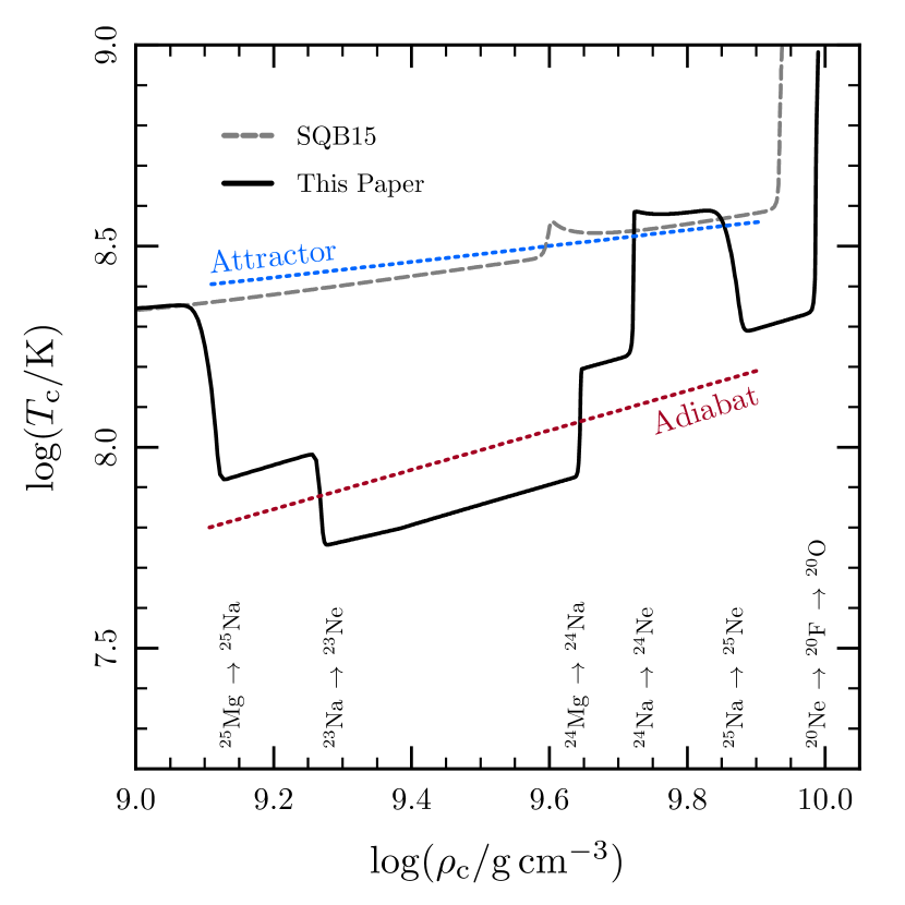
Figure 5: Comparison of a model with (This Paper) and without (SQB15) the isotopes $\mathrm{{}^{23}Na}$ and $\mathrm{{}^{25}Mg}$. The key weak reactions are indicated at the densities at which they occur, accounting only for allowed transitions. The labeled dotted lines show the attractor solution (where neutrino cooling balances compressional heating) and a sample adiabat. These models do not include convection which is, however, likely to occur in models with significant Urca-process cooling (see Section 6).

5 Nonunique second forbidden transitions

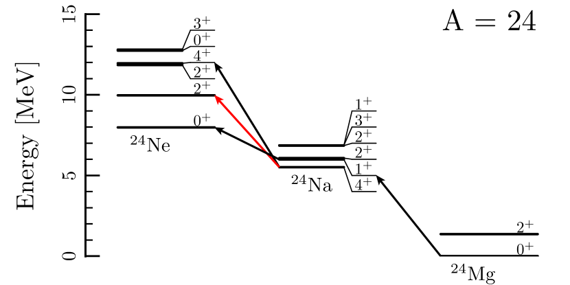
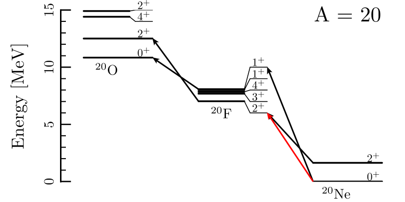
Figure 6: Energy level diagrams for the $A=24$ (left) and $A=20$ (right) nuclei that we consider. The $J^{\pi}$ value is indicated at the right of each level and is sometimes given an arbitrary offset (indicated via a thin line) in order to enhance legibility. The most important transitions we consider are indicated with arrows. The red arrows indicate the nonunique second forbidden transitions (i.e. $\Delta J=2$, $\pi_{i}\pi_{f}=+1$).

In Table 1, we summarized the key weak reactions and gave the threshold density associated with the most important allowed transition. In this section, we discuss the effects of nonunique second forbidden transitions, which are those with $\Delta J=2$, $\pi_{i}\pi_{f}=+1$. Typical $\log(ft/{\rm s})$ values (of beta decays) for nonunique second forbidden transitions are 11.9-13.6 (Raman & Gove, 1973). Such transitions can only dominate the rate when their threshold density is far enough below the threshold density of the allowed transition that the additional phase space can allow it to be more rapid.

Martínez-Pinedo et al. (2014) pointed out the potential importance of the nonunique second forbidden transition between the ground states of $\mathrm{{}^{20}Ne}$ and $\mathrm{{}^{20}F}$. The properties of this transition have not yet been experimentally measured—there exists only an upper limit (Calaprice & Alburger, 1978)—though experiments are being planned (Kirsebom et al., 2017). In SQB15, we explored the effect of this transition and found that while it causes a 0.1 dex shift in the density at which the initial electron captures on $\mathrm{{}^{20}Ne}$ occur, its effect on the central density at the time of oxygen ignition was more modest.

There is also a nonunique second forbidden transition between the ground state of $\mathrm{{}^{24}Na}$ and the first excited state of $\mathrm{{}^{24}Ne}$ (see left panel of Fig. 6). This transition has a threshold density below the threshold density for allowed electron captures from the $\mathrm{{}^{24}Na}$ ground state. The effect of this transition has not previously been explored.

In this work, we follow Martínez-Pinedo et al. (2014) in assuming the phase space shape for these transitions is the same as for the allowed transitions. The shape factor for these non-unique transitions can contain additional powers of the energy, potentially leading to a factor of 10 increase in the rate for the same $ft$ value (Martínez-Pinedo et al., 2014). Since the $ft$ values for these transitions is not measured, we present models with different $ft$ values, and this ambiguity is degenerate with our parameter exploration.

5.1 Effects for $A=24$

The left panel of Fig. 6 shows the key transitions for $A=24$. We now evaluate the relative importance of the allowed transition from the first excited state of $\mathrm{{}^{24}Na}$ to the ground state of $\mathrm{{}^{24}Ne}$ and the nonunique second forbidden transition from the ground state of $\mathrm{{}^{24}Na}$ to the third excited state of $\mathrm{{}^{24}Ne}$.

We want to evaluate the ratio of these rates at the threshold density of the $\mathrm{{}^{24}Mg}\to\mathrm{{}^{24}Na}$ reaction. Using an approximate form of the near-threshold rate (eq. 19 in Martínez-Pinedo et al., 2014) and plugging in the values of the relevant energy levels and their spins, we find

$$\frac{\lambda_{\mathrm{forbidden}}}{\lambda_{\mathrm{allowed}}}\approx 0.7\left[\frac{(ft)_{\mathrm{allowed}}}{(ft)_{\mathrm{forbidden}}}\right]\exp\left(\frac{0.472\,\mathrm{MeV}}{k_{\mathrm{B}}T}\right)$$ (16)

For ratios of the $ft$ values in the range $10^{-8}$ – $10^{-6}$, this means the forbidden transition dominates when $T\lesssim 3-4\times 10^{8}\,\mathrm{K}$. Thus this forbidden transition was already likely not negligible under the conditions encountered in SQB15. In this work, the demonstrated importance of Urca process cooling means that the temperature at the onset of $\mathrm{{}^{24}Mg}$ electron captures is $\log(T/\mathrm{K})\la 8$, and thus the forbidden transition is always important. Electron captures that proceed via the forbidden transition deposit more thermal energy per capture into the plasma; this reflects the difference in the average energy of the captured electron and emitted neutrino.

However, even though this forbidden transition may dominate the rate, it might not necessarily be rapid enough that the conversion of $\mathrm{{}^{24}Na}$ to $\mathrm{{}^{24}Ne}$ will complete before the threshold density rises to the point that the allowed transition from the $\mathrm{{}^{24}Na}$ ground state becomes important. As indicated in Table 1, this occurs at a threshold density of $\log(\rho/\mathrm{g\,cm^{-3}})\approx 9.7$, roughly 0.1 dex above the threshold density for $\mathrm{{}^{24}Mg}$.

Using the compression time estimate from equation (10), it will take approximately $5\dot{M}_{-6}^{-1}\,\mathrm{kyr}$ to achieve this density change. Therefore, electron captures via the allowed transition will be important when the reaction time-scale $\lambda_{\mathrm{forbidden}}^{-1}$ is longer than this compression time-scale. This corresponds to the approximate condition $\log(ft/{\rm s})\gtrsim 15-\log(\dot{M}_{-6})$. Thus, for the expected $ft$ value, the electron captures on $\mathrm{{}^{24}Na}$ will typically not be delayed to higher density.

5.2 Effects for $A=20$

The right panel of Fig. 6 shows the key transitions for $A=20$. Martínez-Pinedo et al. (2014) report that for densities in the range $9.6\la\log(\rho/\mathrm{g\,cm^{-3}})\la 9.9$, the forbidden transition dominates the rate for $\log(T/\mathrm{K})\la 8.8$ (assuming the forbidden transition strength is at its experimental upper limit).

Thus again, while the forbidden transition may dominate the rate, there is not necessarily time for substantial $\mathrm{{}^{20}Ne}$ captures before the threshold density associated with the allowed transition occurs. Performing a similar estimate as in the $A=24$ case gives the approximate condition that the electron captures on the allowed transition will be important when $\log(ft/{\rm s})\gtrsim 13-\log(\dot{M}_{-6})$. This estimate is consistent with the results reported in SQB15. Given that threshold density for the $\mathrm{{}^{25}Na}$-$\mathrm{{}^{25}Ne}$ Urca pair is $\log(\rho/\mathrm{g\,cm^{-3}})\approx 9.8$, when this forbidden transition is important we expect both exothermic $A=20$ electron captures and $A=25$ Urca-process cooling to be operating at the same location in the star.

5.3 Exploration of effects

To explore their effects, we vary the strength of the nonunique second forbidden transitions. For convenience, we choose the two transitions to have the same beta-decay $ft$ value. We run models with values $\log(ft/{\rm s})=$ 11, 13 and 15, setting the $ft$ values for electron capture correspondingly, including the ratio of the spin degeneracies. There is no physical reason that the transitions need to have the same strength. However, for the models shown in Fig. 7, the star returns to the “attractor” solution between the $A=24$ and $A=20$ electron captures, largely erasing the previous effects. Therefore, one can roughly assess the effects of each transition independently.

The tracks shown in Fig. 7 agree with the estimates in the previous subsections as to when the each of the transitions is important. The nonunique second forbidden transition in $\mathrm{{}^{24}Na}$-$\mathrm{{}^{24}Ne}$ determines whether the $\mathrm{{}^{24}Na}$ electron captures occur immediately after those on $\mathrm{{}^{24}Mg}$ or whether they are delayed to higher density, but does not appear to have an effect on the subsequent evolution. However, given the important role that the $A=24$ electron captures play in the onset of convective instability (see Section 6), such a delay could in principle have an effect that would not be revealed by the models in this paper. When the nonunique second forbidden transition in $\mathrm{{}^{20}Ne}$-$\mathrm{{}^{20}F}$ is important ($\log(ft/{\rm s})\la 13$), we do not see a significant dependence of the ignition density on the strength of the transition. When this transition is unimportant ($\log(ft/{\rm s})\approx 15$), then the Urca-process cooling by $\mathrm{{}^{25}Na}$-$\mathrm{{}^{25}Ne}$ at $\log(\rho/\mathrm{g\,cm^{-3}})\approx 9.85$ significantly cools the material and leads to electron captures on $\mathrm{{}^{20}Ne}$ that begin at slightly higher density ($\approx 0.05$ dex) than the other models.

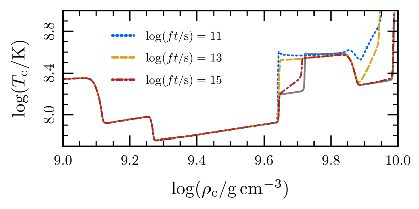
Figure 7: Models with a range of $ft$ values for the uncertain nonunique second forbidden transitions. The grey line shows a model which only includes allowed transitions. At this accretion rate, $\dot{M}=10^{-6}\,\mathrm{\rm\mathrm{M}_{\sun}\,yr^{-1}}$, the nonunique second forbidden transitions are only negligible if $\log(ft/{\rm s})\ga 15$.

6 Stability during and after the electron captures on $\mathrm{{}^{24}Mg}$ and $\mathrm{{}^{24}Na}$

Previous models of accreting ONe WDs have found that the WD remains convectively stable when using the Ledoux criterion for convection (Miyaji et al., 1980; Miyaji & Nomoto, 1987; Canal et al., 1992; Hashimoto et al., 1993; Gutierrez et al., 1996; Gutiérrez et al., 2005). Even though the entropy release from the electron captures creates a highly superadiabatic temperature gradient, it does not trigger convection because of the stabilizing $Y_{\mathrm{e}}$-gradient.

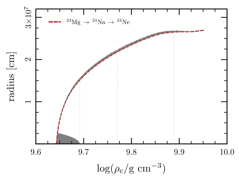
Figure 8: Location of convectively unstable regions in the fiducial model. On the $x$-axis, $\log(\rho_{\mathrm{c}}/\mathrm{g\,cm^{-3}})$ serves as a proxy for time. The dashed line shows the location of the $A=24$ electron capture front (defined by the place where the $\mathrm{{}^{24}Mg}$ and $\mathrm{{}^{24}Ne}$ abundances are approximately equal). The grey shaded regions show where $N^{2}<0$. The action of convection has been artificially suppressed in this model; no mixing occurs in convectively unstable regions.

The MESA models in this paper, which are the first to include the effects of significant Urca-process cooling, do develop regions of convective instability. In regions where the electron captures are occurring, and thus where the temperature and $Y_{\mathrm{e}}$ gradients are necessarily tightly linked, the material remains convectively stable, consistent with previous results. However, our models show the development of convectively unstable regions (i.e. where $N^{2}<0$) in the core after the $A=24$ electron captures have completed and also off-centre, ahead of the region where the $A=24$ electron captures are occurring. Fig. 8 shows the convectively unstable regions in our fiducial model. In these models, we evaluate convective instability via the Ledoux criterion, but suppress the action of convection once unstable regions develop (see Section 4.2 for the MESA options used).

These results indicate that the temperature of the material immediately before it undergoes the $A=24$ electron captures has a profound effect on the convective stability of the model. This temperature dependence is a consequence of the steep temperature dependence of the electron capture reactions and the subsequent influence of thermal conduction.

As material in the centre of the WD nears the threshold density, the electron-capture reaction rates increase and the reactions will proceed in earnest once the reaction time-scale is of order the compression time-scale. This happens while the reaction is still sub-threshold, meaning the reaction rate has an exponential dependence on the temperature. This strong temperature dependence allows for a thermal runaway.

The initial length scale for the runaway is set by hydrostatic equilibrium. The core is approximately isothermal, but the pressure decreases with increasing radius. This implies a gradient in the electron chemical potential and thus a length scale over which the electron capture rate (and hence the heating rate) varies by order unity. Recall that in the sub-threshold limit the rate varies with temperature as

$$\lambda\propto\left(\frac{k_{\mathrm{B}}T}{m_{\mathrm{e}}c^{2}}\right)^{3}\exp\left(\frac{\mu+Q}{k_{\mathrm{B}}T}\right)~{}.$$ (17)

So the rate varies by a factor of $e$ over a length scale where the chemical potential changes by $\Delta\mu=k_{B}T$. Since the thermal contribution to the pressure is not significant, the variation of the chemical potential is roughly independent of the temperature, meaning the length scale of this variation in the rate is smaller at lower temperatures.

Additionally, at a lower initial temperature, for the reaction rate to reach a given value, the material must get closer to the threshold density (i.e. $(\mu+Q)/(k_{\mathrm{B}}T)$ will be less negative). This means that once the temperature rises as a result of the heating, the reaction rate is faster at a given temperature. This means that the thermal runaway will complete in a shorter amount of time.

Fig. 9 shows temperature profiles during the runaway for a model that has not experienced Urca-process cooling (top) and one that has (bottom). The two most important differences are readily apparent: the length scale of the initially colder runaway is significantly smaller and the runaway completes in substantially less time. In the SQB15 model, the longer time means that thermal neutrino cooling is more important; this effect explains why the central temperature is not at the maximum temperature in the final profile shown in the top panel.

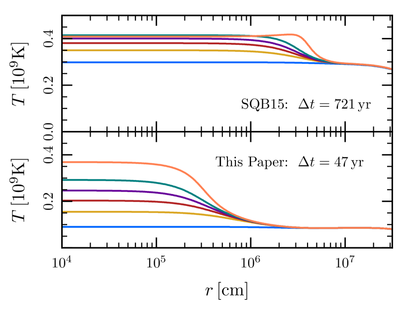
Figure 9: Temperature profiles during the thermal runaway caused by the $A=24$ electron captures. The top panel shows a model that did not include earlier Urca-process cooling and hence is significantly hotter than the bottom panel which did include Urca-process cooling. Profiles are shown at times when the central $\mathrm{{}^{24}Mg}$ mass fraction is 0.0495, 0.04, 0.03, 0.02, 0.01, and 0.0005. (The temperature increases as $\mathrm{{}^{24}Mg}$ is consumed.) The annotation indicates the time elapsed between first and last profile shown. The runaway that begins at an initially colder temperature has a smaller length scale and time-scale. None of the profiles shown are convectively unstable, though instability will shortly set in for the model in the bottom panel.

The thermal runaway associated with the $A=24$ electron captures ends because of the exhaustion of $\mathrm{{}^{24}Mg}$. This is the key difference between this runaway and the $\mathrm{{}^{20}Ne}$ runaway that we studied in detail in SQB15, where thermonuclear oxygen begins before $\mathrm{{}^{20}Ne}$ depletion. As the runaway ends and each parcel reaches the post-capture composition, no residual composition gradient remains. However, a residual temperature gradient does remain because of the slight gradient in the reaction rate and the differential effects of thermal conduction. This residual temperature gradient is superadabiatic and thus the material is convectively unstable. This produces a central convection zone on the length scale of the initial thermal runaway, as shown in Fig. 8. In Appendix C, we reproduce this behavior in a simple toy model.

The thermal runaway produces a small hotspot at the centre of the star. Heat from this hotspot will be conducted outwards, but this cannot lead to the propagation of the electron-capture front through a significant portion of the star, since the reactions only occur in material near or above the threshold density. Therefore, as in previous models, the electron-capture front moves outwards as a consequence of accretion.

The front is advancing slowly, moving through the star on the compression time-scale, and so conduction can move heat ahead of it. Ahead of the front, where the chemical potential is lower, the electron-capture reactions are sufficiently slow that an increase in the temperature does not result in significant composition change. Thus in these regions a temperature gradient develops without a corresponding $Y_{\mathrm{e}}$ gradient and the region becomes convectively unstable. Models that have experienced Urca process cooling are more prone to experience this because their steeper temperature gradients favor conduction and because with a lower upstream temperature less heat is required to get a super-adiabatic temperature gradient.

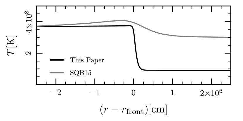
Figure 10: Temperature profiles near the $A=24$ electron-capture front in the fiducial model and the model from SQB15 (shown at the time when $\log(\rho_{\mathrm{c}}/\mathrm{g\,cm^{-3}})=9.7$). The lower upstream temperature due to Urca cooling causes the temperature gradient to be much steeper, enhancing the destabilizing effects of thermal conduction.

If we allow convection to operate via the usual mixing length theory (MLT), it becomes extremely difficult for MESA to proceed and we have not been able to construct numerically-converged MESA models beyond this point. When a zone becomes convectively unstable, its temperature gradient changes from the radiative gradient to the adiabatic gradient. These temperature changes affect the structure in a way that alters the convective stability of other zones. As MESA iterates to find the new solution, the convective boundaries change at each iteration and the solver fails to converge.

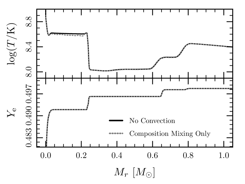
Figure 11: Comparison of temperature (top panel) and composition (bottom panel) profiles for models at the time of oxygen ignition. The model with no convection and the model in which convection only mixes composition (but does not modify temperature) agree well. This indicates that if the convection zones do not grow, they will not substantially affect the evolution of the models.

As a demonstration that it is the temperature change that causes the problem (at least initially), and not the composition mixing, we ran a model that does not allow MLT to change the temperature, but retains the normal MLT diffusion coefficients for mixing of composition (see Section 4.2 for the MESA options used). Fig. 11 compares this model (at the time of oxygen ignition) with our fiducial model in which convection is completely suppressed. No significant difference exists between the two models. Physically, the regions that become unstable are ahead and behind the electron-capture front in regions that do not have substantial composition gradients. Thus composition mixing in these regions cannot by itself have a significant effect.

The essential question that must be answered about these convectively unstable regions is: do they want to grow? In particular, do they grow and ultimately lead to the formation of a long-lived central convection zone? Previous work has demonstrated the qualitative difference between models that develop a convective core and those that don’t (Miyaji et al., 1980; Miyaji & Nomoto, 1987). The presence of a central convection zone means the heating from the electron captures is effectively deposited over the entire convective region. With a greater mass to heat, more material must undergo electron captures to cause the core to reach conditions for oxygen ignition. Models with central convection zones at the onset of $\mathrm{{}^{20}Ne}$ captures do not reach oxygen ignition until much higher densities, strongly favoring their collapse to form a neutron star.

However, the evolution of models with large central convection zones is subject to the substantial uncertainties associated with the convective Urca process (Paczyński, 1972). Once the convection zone grows to span the threshold density of one or more of the Urca pairs, convective motions can transport material that has undergone electron captures in higher density regions to lower density regions where it will beta decay (and vice-versa). The greater abundances of Urca-pair isotopes in ONe WDs (compared to CO WDs) will increase the importance of this process. The interaction of the convective mixing and the reactions is difficult to model. The development of a treatment for the convective Urca process and its effects suitable for inclusion in stellar evolution codes remains an active area of research (e.g. Lesaffre et al., 2005).

Therefore, it is non-trivial but of critical importance to explore the outcome of these convectively unstable regions and how to best model them in stellar evolution codes. We necessarily defer this difficult problem to future work.

7 Subsequent evolution towards collapse

Section 6 demonstrated the onset of localized convective instability after the $A=24$ electron captures begin. Uncertainties in how to treat the evolution at this point mean that the later evolution is necessarily less certain. For now, we proceed by artificially suppressing the action of convection. This allows us to characterize the evolution of models in which a long-lived central convection zone does not develop.

7.1 Onset of electron captures on $\mathrm{{}^{20}Ne}$ and $\mathrm{{}^{20}F}$

As discussed in SQB15, the electron captures on $\mathrm{{}^{20}Ne}$ trigger a thermal runaway that leads to the formation of an outgoing oxygen deflagration wave. The final fate of the star is determined by a competition between the propagation of the oxygen deflagration and electron captures on the material (in nuclear statistical equilibrium; NSE) behind the deflagration front (Nomoto & Kondo, 1991). The speed of the deflagration and the electron capture rate on its NSE ash are both functions of density and electron fraction. Timmes & Woosley (1992) found that the deflagration speed scaled $\propto\rho^{1.06}$. At the relevant densities, the neutronization time-scale scales roughly as $\rho^{-0.5}$ (see figure 13 in SQB15 and Seitenzahl et al., 2009). Studies of the final fate of these objects typically explore uncertainties in the initial models by varying the central density at oxygen ignition (e.g. Jones et al., 2016). Therefore, we now describe the range of central densities found in our models.

The temperature affects the density at which the electron captures on $\mathrm{{}^{20}Ne}$ begin, with lower temperatures corresponding to higher densities (see figure 4 in SQB15), so Urca-process cooling can influence the ignition density. In Fig. 7, we showed that if the nonunique second forbidden transition is unimportant ($\log(ft/{\rm s})\approx 15$), then the Urca-process cooling by $\mathrm{{}^{25}Na}$-$\mathrm{{}^{25}Ne}$ at $\log(\rho/\mathrm{g\,cm^{-3}})\approx 9.85$ effectively sets the temperature at which the electron captures on $\mathrm{{}^{20}Ne}$ begin. This leads to electron captures on $\mathrm{{}^{20}Ne}$ that begin at slightly higher density ($\approx 0.05$ dex) than in SQB15. In cases where this forbidden transition is important ($\log(ft/{\rm s})\la 13$), we do not see a significant dependence of the ignition density on the details of the transition.

The composition could also influence the ignition density. We do not perform an extensive parameter study, but Fig. 12 shows the evolution of the central density and temperature for the representative compositions listed in Table 2. We see minor differences between the evolutionary tracks. For example, the F15 models have the lowest abundance of $A=25$ elements and this accounts for the differences in cooling around $\log(\rho/\mathrm{g\,cm^{-3}})\approx 9.1$ and $9.85$. However, the density at which electron captures on $\mathrm{{}^{20}Ne}$ trigger oxygen ignition is insensitive to the precise details of the composition.

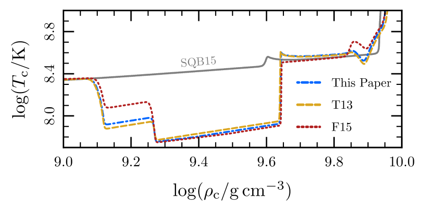
Figure 12: Comparison of a model with our fiducial composition (This Paper) with two compositions based on recent results of the evolution of intermediate mass stars: (T13; Takahashi et al., 2013) and (F15; Farmer et al., 2015). The solid line shows the model from SQB15. The precise compositions are given in Table 2. While the details of the evolution depend on the abundances, the density at which electron captures on $\mathrm{{}^{20}Ne}$ trigger the oxygen deflagration appears to be insensitive to the precise composition. The density is only slightly higher $(\approx 0.02$ dex) than the model in SQB15. All models neglect convection.

7.2 Propagation of the oxygen deflagration

Independent of their cooling effects, the electron captures on $\mathrm{{}^{23}Na}$, $\mathrm{{}^{25}Mg}$, and $\mathrm{{}^{25}Na}$ have reduced the $Y_{\mathrm{e}}$ of the material. For the fiducial composition, this change is $\Delta Y_{\mathrm{e}}\approx-3\times 10^{-3}$. A reduction in $Y_{\mathrm{e}}$ increases both of the oxygen deflagration speed and the electron-capture rates on the oxygen burning ashes. Timmes & Woosley (1992) found that reducing $Y_{\mathrm{e}}$ from 0.50 to 0.48 reduced the deflagration speed by approximately 30 per cent. In the tabulated electron-capture rates on NSE material from Seitenzahl et al. (2009), changing $Y_{\mathrm{e}}$ from 0.50 to 0.48 at $\log(\rho/\mathrm{g\,cm^{-3}})\approx 9.9$ and $\log(T/\mathrm{K})\approx 10$ increases the neutronization time-scale by approximately a factor of 2.5. Note that these changes are quoted for a $\Delta Y_{\mathrm{e}}$ approximately 10 times greater than the difference here.

The exact competition between these two processes is best probed via simulations which can include both the physics of the oxygen deflagration and the NSE electron captures. However, the changes due to a possible increase in density and the decrease in $Y_{\mathrm{e}}$ are relatively small and in opposite directions; they are unlikely to significantly affect the fate of the outwardly-going oxygen flame.

7.3 Other effects of reduced electron fraction

The electron captures on the A=23 and A=25 isotopes reduce $Y_{\mathrm{e}}$ in the material in the WD that has exceeded the threshold density for these reactions. At oxygen ignition, this has occurred in about half of the star (see Fig. 11). The Chandrasekhar mass scales with $Y_{\mathrm{e}}^{2}$, and so at the onset of collapse, models which experience this reduction in $Y_{\mathrm{e}}$ will have lower masses relative to models in which these composition shifts have not been accounted for.

The models shown in Fig. 5 have different masses at the time of the formation of the oxygen deflagration (and hence the likely collapse to a NS). The mass difference between these two models is $\approx 0.016$ $\mathrm{M}_{\sun}$, with the model that included the odd mass number isotopes having the lower mass. Studies that use the observed mass of low-mass neutron stars (thought to be formed via AIC or electron-capture supernova) to make inferences about the nuclear equation of state (e.g. Podsiadlowski et al., 2005) require knowing the baryonic mass of the WD just prior to collapse. A mass difference of $0.01\,\mathrm{\mathrm{M}_{\sun}}$ is the same order of magnitude as the effects of finite temperature, general relativity, and Coulomb corrections, which are important in formulating such constraints. To realize the suggestion of Podsiadlowski et al. (2005) that one can ultimately pinpoint the baryonic mass of the core to within $2\times 10^{-3}\,\mathrm{\mathrm{M}_{\sun}}$ will require realistic temperature and composition profiles.

8 Effect of accretion rate

In Sections 4-7 we focused on models accreting at a constant rate of $\dot{M}=10^{-6}\,\mathrm{\rm\mathrm{M}_{\sun}\,yr^{-1}}$. Near the Chandrasekhar mass $(\ga 1.3\mathrm{M}_{\sun})$, the range of mass accretion rates for thermally-stable hydrogen burning is $\approx 4-7\times 10^{-7}\,\mathrm{\rm\mathrm{M}_{\sun}\,yr^{-1}}$ (Wolf et al., 2013) and for thermally-stable helium burning is $\approx 1.5-4.5\times 10^{-6}\,\mathrm{\rm\mathrm{M}_{\sun}\,yr^{-1}}$ (Brooks et al., 2016). Thus our fiducial choice represents an accretion rate that is approximately characteristic of any stably-burning accretor. However, it is useful to repeat the models for a range of accretion rates; such a parameter study was presented in SQB15 and we now update that result including the effects of the Urca process.

As discussed in Section 3, at lower accretion rates, the WD will be cooler. This is because the longer compression time-scale means the balance between compressional heating and thermal neutrino losses occurs at lower temperature; additionally, once the Urca-process neutrino cooling occurs it will cool material to a lower temperature. Fig. 13 shows the evolution of the central conditions for models with several accretion rates and both of these effects are evident.

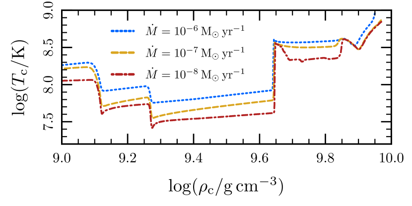
Figure 13: Central density-temperature trajectories of models with different accretion rates. Models with lower accretion rates have lower temperature, but the overall evolution is similar.

In a cooler WD, the physical width of the regions over which the weak reactions primarily occur will be narrower (since the extent scales $\propto k_{\mathrm{B}}T/E_{\mathrm{F}}$). Both the longer compression time-scale and the shorter lengthscale serve to enhance the relative importance of thermal conduction. Fig. 14 plots $T$ and $Y_{\mathrm{e}}$ profiles for the models shown in Fig. 13 at the time of oxygen ignition. The effects of thermal diffusion can be seen in the shallower temperature gradients. This is particularly easy to see around $\log(\rho/\mathrm{g\,cm^{-3}})\approx 9.6$ in the model with $\dot{M}=10^{-8}\,\mathrm{\rm\mathrm{M}_{\sun}\,yr^{-1}}$, where it is evident that substantial heat from the $A=24$ electron captures has diffused to lower density. Consistent with this fact, in models with lower accretion rates we observe larger regions that are convectively unstable due to the effect discussed in Section 6.

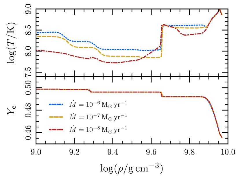
Figure 14: Temperature (top panel) and composition (bottom panel) profiles at the time of oxygen ignition for models with different accretion rates.

As noted in SQB15, the non-unique second forbidden transition can lead to mildly off-centre ignitions if its strength is near the experimental upper limit (see figure 12 and surrounding discussion). As can be seen in Fig. 13 and Fig. 14, the models with $\dot{M}$ of $10^{-7}\,\mathrm{\rm\mathrm{M}_{\sun}\,yr^{-1}}$ and $10^{-8}\,\mathrm{\rm\mathrm{M}_{\sun}\,yr^{-1}}$ experience mildly off-centre ignitions with the fiducial transition strength of $\log(ft/{\rm s})=11$. This shows that at a fixed transition strength, lower accretion rates lead to off-centre ignitions. When an off-centre ignition does occur, the ignition location is $\la 50\,\mathrm{km}$ from the centre of the WD. Given the uncertainties in the strength of the non-unique second forbidden transition, we defer a more thorough characterization of this effect to future work.

9 Conclusions

We have demonstrated the substantial effects that Urca-process cooling has on the thermal evolution of accreting ONe WDs. We have provided a simple analytic expression for the peak Urca-process cooling rate (equation 6) and used it to derive an approximate expression for the temperature to which the Urca process cools the plasma (equation 15). We used a suite of MESA simulations to confirm these simple analytic scalings (Figs. 3 and 4). The magnitude of these effects is inconsistent with earlier work by Gutiérrez et al. (2005), who severely underestimate the amount of Urca-process cooling.

As discussed by Paczyński (1973), Urca-process cooling will also occur in accreting CO WDs, where it leads to an increase in the density at which carbon is ignited. This effect has not been fully explored in the context of Type Ia supernova progenitors. The estimates we provide in Section 3 are equally applicable in this case (Denissenkov et al., 2015; Martínez-Rodríguez et al., 2016; Piersanti et al., 2017)

In Section 5 we characterized the effects of two nonunique second forbidden transitions. Since the strength of these transitions has not yet been experimentally measured, we characterized their effect for a range of transition strengths (Fig. 7). One transition, in $\mathrm{{}^{20}Ne}$-$\mathrm{{}^{20}F}$, has been previously discussed by Martínez-Pinedo et al. (2014) and SQB15. In this paper we showed that this transition is important at the same density where cooling from the $\mathrm{{}^{25}Na}$-$\mathrm{{}^{25}Ne}$ Urca pair is occurring. The other transition, in $\mathrm{{}^{24}Na}$-$\mathrm{{}^{24}Ne}$, has not previously been discussed; we find it does appear to be important in determining the rate. Given the role the $A=24$ electron captures play in causing convective instability, it would be desirable to better measure this transition strength.

In Section 6 we showed that Urca-process cooling has another important consequence. It leads to lower temperatures at the onset of $A=24$ captures in turn producing convectively unstable regions, even when using the Ledoux criterion. In Section 6 and Appendix C, we explained how thermal conduction leads to this outcome. Numerical difficulties associated with the development of these convectively unstable regions prevented us from evolving the models further while modeling convection using normal mixing length theory. We showed that if the convection zones mix only localized regions, their effect on the subsequent evolution is minimal. However, if these convection zones were to grow to encompass a significant fraction of the star, their effect on its evolution would be profound; models that have large convective cores undergo collapse at significantly higher density (Miyaji et al., 1980). Understanding the dynamics of these convection zones will be an important avenue for future work. Multi-dimensional hydrodynamics simulations may be able to help determine whether these convection zones want to grow. Useful results may also be obtained from stellar evolution calculations using mixing prescriptions that circumvent the numerical difficulties encountered in this work.

In Section 7 we continued to evolve our models up to the onset of oxygen ignition, under the assumption that the convectively unstable regions do not substantially alter the structure of the WD. We find similar central densities at the time of oxygen ignition as SQB15. This suggests that inclusion of Urca-process cooling does not affect the conclusion that the final outcome of accreting ONe WDs approaching the Chandrasekhar mass is accretion-induced collapse to a neutron star (Nomoto & Kondo, 1991). However, this conclusion is provisional given the uncertainties introduced by convection. In addition, recent multi-dimensional work has begun to revisit the critical density threshold (Jones et al., 2016). Future work using hydrodynamical models and realistic progenitor models can help elucidate whether aspects such as the different $Y_{\mathrm{e}}$ profiles have an effect on the collapse.

Appendix A Maximum Urca Cooling Rate

The expressions for the rates of electron-capture and beta-decay reactions have been previously derived (e.g. Tsuruta & Cameron, 1970; Fuller et al., 1985; Martínez-Pinedo et al., 2014). In this Appendix, for completeness, we give expressions for these rates, specialized to the Urca process, with the goal of extracting a simple expression for the maximum Urca-process cooling rate. We consider only the allowed ground state to ground state transition of an Urca pair. We choose the isotope undergoing electron capture to have charge $Z$ and thus the isotope undergoing beta decay has charge $Z-1$. We always assume the electrons are relativistic with energy $E_{\mathrm{e}}\gg m_{\mathrm{e}}c^{2}$.

The rate of electron capture or beta decay can be written as

$$\lambda=\frac{\ln 2}{(ft)}I(\mu,T,Q),$$ (18)

where $ft$ is the comparative half-life (typically given in units of seconds) and can be either measured experimentally or theoretically calculated from the weak-interaction nuclear matrix elements. The phase space factor $I$ depends on the temperature $T$, electron chemical potential $\mu$, and the energy difference between the parent and daughter states $Q$. The value of $Q$ includes both the nuclear rest mass and the energy associated with excited states. Similarly, the rate of energy loss via neutrinos is

$$\varepsilon_{\nu}=\frac{m_{\mathrm{e}}c^{2}\ln 2}{(ft)}J(\mu,T,Q)~{},$$ (19)

where $J$ is a phase space factor that contains an additional power of the neutrino energy.

For convenience, we define $\beta=(k_{B}T)^{-1}$ and the non-dimensionalized parameters $q=\beta|Q|$, $\theta=\beta m_{\mathrm{e}}c^{2}$, $\eta=\beta\mu$, $\epsilon=\beta E_{\mathrm{e}}$. The value of $I$ for electron capture is

$$I_{\mathrm{ec}}=\theta^{-5}\exp(\pi\alpha Z)\int_{q}^{\infty}\frac{\epsilon^{2}(\epsilon-q)^{2}}{1+\exp(\epsilon-\eta)}d\epsilon~{},$$ (20)

and the value of $J$ for electron capture is

$$J_{\mathrm{ec}}=\theta^{-6}\exp(\pi\alpha Z)\int_{q}^{\infty}\frac{\epsilon^{2}(\epsilon-q)^{3}}{1+\exp(\epsilon-\eta)}d\epsilon~{},$$ (21)

where $\alpha$ is the fine structure constant. These integrals can easily be rewritten (using the substitution $x=\epsilon-q$) in terms of the complete Fermi integrals, which are defined as

$$F_{k}(y)=\int_{0}^{\infty}\frac{x^{k}}{1+\exp(x-y)}dx~{}.$$ (22)

Doing so gives

$$I_{\mathrm{ec}}=\theta^{-5}\exp(\pi\alpha Z)\left[F_{4}(\delta)+2qF_{3}(\delta)+q^{2}F_{2}(\delta)\right]~{},$$ (23)

and

$$J_{\mathrm{ec}}=\theta^{-6}\exp(\pi\alpha Z)\left[F_{5}(\delta)+2qF_{4}(\delta)+q^{2}F_{3}(\delta)\right]~{},$$ (24)

where we have defined $\delta=\eta-q$.

The value of $I$ for beta decay can be written as

$$I_{\beta}=\theta^{-5}\exp(\pi\alpha Z)\int_{\theta}^{q}\frac{\epsilon^{2}(\epsilon-q)^{2}}{1+\exp[-(\epsilon-\eta)]}d\epsilon~{},$$ (25)

and the value of $J$ for beta decay can be written as

$$J_{\beta}=\theta^{-6}\exp(\pi\alpha Z)\int_{\theta}^{q}\frac{\epsilon^{2}(\epsilon-q)^{3}}{1+\exp[-(\epsilon-\eta)]}d\epsilon~{}.$$ (26)

These integrals can be rewritten (using the substitution $x=-\epsilon+q$) to be

$$I_{\beta}=\theta^{-5}\exp(\pi\alpha Z)\int_{0}^{q-\theta}\frac{(x-q)^{2}x^{2}}{1+\exp[x-(q-\eta)]}d\epsilon~{},$$ (27)

and

$$J_{\beta}=\theta^{-6}\exp(\pi\alpha Z)\int_{0}^{q-\theta}\frac{(x-q)^{2}x^{3}}{1+\exp[x-(q-\eta)]}d\epsilon~{}.$$ (28)

We can now make use of the identity

$$\int_{0}^{b}\frac{x^{k}}{1+\exp(x-y)}=F_{k}(y)-\sum_{j=0}^{k}\binom{k}{j}b^{k-j}F_{j}(y-b)~{},$$ (29)

where we identify $y=q-\eta$ and $b=q-\theta$. The Fermi integrals in the sum (those with argument $y-b$) will be negligible because $\theta-\eta\ll-1$ and $F_{k}(-z)\propto\exp(-z)$. In other words, we can extend the upper limit to $\infty$ without incurring substantial error. Doing so gives

$$I_{\beta}=\theta^{-5}\exp(\pi\alpha Z)\left[F_{4}(-\delta)-2qF_{3}(-\delta)+q^{2}F_{2}(-\delta)\right]~{},$$ (30)

and

$$J_{\beta}=\theta^{-6}\exp(\pi\alpha Z)\left[F_{5}(-\delta)-2qF_{4}(-\delta)+q^{2}F_{3}(-\delta)\right]~{},$$ (31)

where we have again defined $\delta=\eta-q$.

We are interested in the expression

$$C=\frac{\varepsilon_{\nu,\mathrm{ec}}\lambda_{\beta}+\varepsilon_{\nu,\beta}\lambda_{\mathrm{ec}}}{\lambda_{\beta}+\lambda_{\mathrm{ec}}}=m_{\mathrm{e}}c^{2}\ln(2)\left(\frac{I_{\mathrm{ec}}J_{\beta}+I_{\beta}J_{\mathrm{ec}}}{(ft)_{\beta}I_{\mathrm{ec}}+(ft)_{\mathrm{ec}}I_{\beta}}\right)~{}.$$ (32)

The limit of interest is $q\gg 1$ and $|\delta|<1$. Recall that for $y\ll 1$, $F_{k}(y)\approx-y\Gamma(k+1)$. Therefore, after retaining the dominant terms,

$$C=m_{\mathrm{e}}c^{2}\ln(2)\theta^{-6}q^{2}\exp({\pi\alpha Z})\left[\frac{F_{2}(\delta)F_{3}(-\delta)+F_{2}(-\delta)F_{3}(\delta)}{(ft)_{\beta}F_{2}(\delta)+(ft)_{\mathrm{ec}}F_{2}(-\delta)}\right]~{}.$$ (33)

Evaluating the term in square braces at $\delta=0$ gives

$$C=\frac{m_{\mathrm{e}}c^{2}\ln 2}{(ft)}\theta^{-6}q^{2}\exp({\pi\alpha Z})\left[\frac{7\pi^{4}}{60}\frac{1}{(ft)_{\beta}+(ft)_{\mathrm{ec}}}\right].$$ (34)

and the peak value of the Urca-process cooling rate is thus

$$C_{\mathrm{max}}=\frac{7\pi^{4}\ln 2}{60}\frac{m_{\mathrm{e}}c^{2}}{(ft)_{\beta}+(ft)_{\mathrm{ec}}}\left(\frac{k_{\mathrm{B}}T}{m_{\mathrm{e}}c^{2}}\right)^{4}\left(\frac{Q}{m_{\mathrm{e}}c^{2}}\right)^{2}\exp({\pi\alpha Z})~{}.$$ (35)

Assuming $(ft)_{\beta}=(ft)_{\mathrm{ec}}$, which is true when the ground states have the same spins, we can Taylor expand the term in square braces in equation (33) to second order to obtain the dependence of $C$ on $\delta$, the dimensionless energy difference away from threshold:

$$C\propto\frac{1}{(ft)}\left[\frac{7\pi^{4}}{120}-\frac{\pi^{2}\delta^{2}}{4}\right].$$ (36)

The term in square braces is zero when $\delta=\sqrt{7/30}\pi$, implying that the characteristic width of the Urca-process cooling peak is $\approx 3\delta$, that is when $\mu\approx|Q|\pm 1.5k_{\mathrm{B}}T$.

Appendix B Convergence

In order for the results of our MESA calculations to be meaningful, we must ensure that the resolution (in both space and time) is sufficient to resolve the processes of interest. Once that condition is achieved, we must also demonstrate that the answer is independent of the resolution.

The overall spatial and temporal convergence settings used in our MESA calculations are

    varcontrol_target = 1e-3
    mesh_delta_coeff = 1.0

Because the weak reactions produce temperature and composition changes, the default controls typically do an acceptable job of spatially resolving the cooling and heating regions. However, the effective timestep limit in a run with these controls alone is typically due to the Newton-Raphson solver taking an excessive number of iterations to converge and MESA limiting the timestep in response. It is more satisfying to limit the timestep based on a physical criteron. In SQB15, we demonstrated that this value of varcontrol_target, along with a timestep criterion based on changes in central density

    delta_lgRho_cntr_hard_limit = 3e-3
    delta_lgRho_cntr_limit = 1e-3

gave a converged result. In this Appendix, we demonstrate that this is still true when including Urca-process cooling, and we adopt these as our fiducial resolution controls.

From Section 2 and equation (36) above, we know that the Urca-process cooling occurs over a range corresponding to a change in Fermi energy $\Delta E_{\mathrm{F}}\sim k_{\mathrm{B}}T$. MESA calculates the value of the quantity $\eta=(k_{\mathrm{B}}T/E_{\mathrm{F}})^{-1}$ in each cell at each timestep. If we ensure the mesh points in our model are selected as to limit variation of $\Delta\eta$ between adjacent cells and ensure that our timestep is such that $\delta\eta$ in a given cell between timesteps is also limited, we will resolve the Urca process.

The scheme by which the spatial resolution in MESA is modified is described in section 6.5 of Paxton et al. (2011). MESA allows the user to specify other “mesh functions” whose cell-to-cell variation will be reduced below the value of mesh_delta_coeff during remeshes. Therefore, we define one of the mesh functions to be $f_{1}=\eta/\Delta\eta_{\mathrm{limit}}$. Then MESA will limit the change in $\eta$ between adjacent cells $k$ and $k+1$ at timestep $i$,

$$\Delta\eta=\left|\eta_{k+1}^{i}-\eta_{k}^{i}\right|~{},$$ (37)

to be less than $\Delta\eta_{\mathrm{limit}}$.

We similarly limit the timestep. After the solver has taken the values at timestep $i$ and returned a proposed solution at timestep $i+1$, we calculate the change in $\eta$ in each cell $k$ and take the maximum,

$$\delta\eta=\max\left(\left|\eta_{k}^{i+1}-\eta_{k}^{i}\right|\right)~{}.$$ (38)

If $\delta\eta>\delta\eta_{\mathrm{limit}}$, then the proposed step is rejected and redone with a shorter timestep. This is similar to the way variations in the structure variables are limited via varcontrol_target.

We vary the spatial and temporal parameters and check that our results are unaffected. We use the same model as in Fig. 2, one composed of $\mathrm{{}^{16}O}$, $\mathrm{{}^{20}Ne}$, and $\mathrm{{}^{23}Na}$ (with $X_{\mathrm{Na}}=0.01$). Fig. 15 compares a run with the limits $\Delta\eta_{\mathrm{limit}}=1$ and $\delta\eta_{\mathrm{limit}}=1$ to our fiducial resolution controls, which limit the change in central density as in SQB15. The results of the fiducial and high resolution cases are nearly indistinguishable in the quantities of interest, demonstrating that our results are converged.

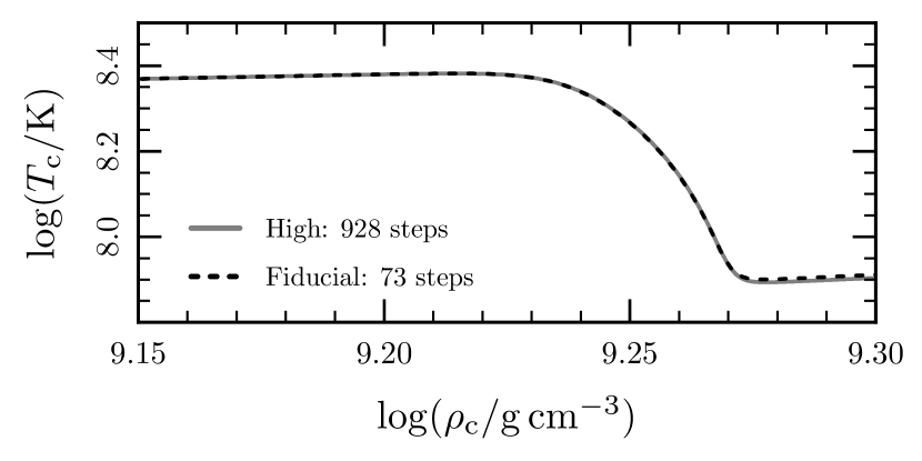
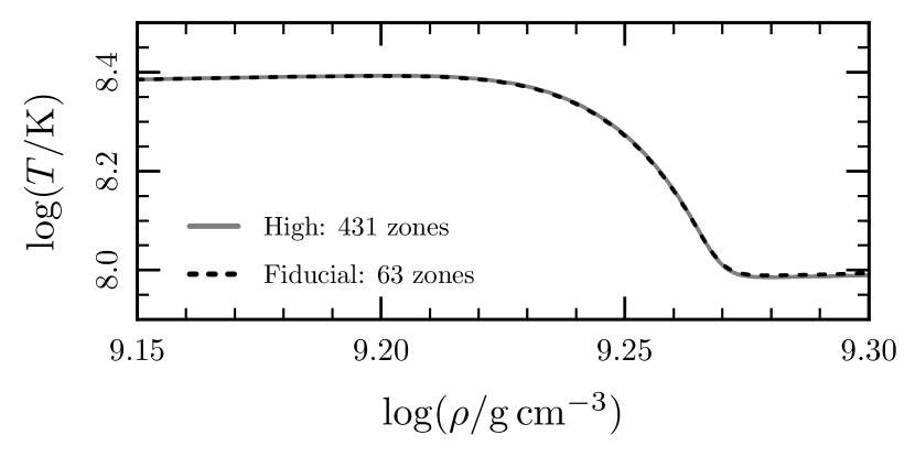
Figure 15: The evolution of a model with $X_{\mathrm{Na}}=0.01$ using the different resolution controls discussed in the text. The top panel shows the evolution of the central density and temperature. The legend shows the number of timesteps used to go from the (local) maximum temperature to the (local) minimum temperature. The bottom panel shows the density and temperature profile of the model when $\log(\rho_{\mathrm{c}}/\mathrm{g\,cm^{-3}})=9.4$. The legend shows the number of mesh points covering the region from the (local) maximum temperature to the (local) minimum temperature.

Appendix C Toy Model of Runaway

In order to gain insight into the behavior observed in our MESA calculations, we use a toy model of a thermal runaway process. We solve a reaction-diffusion equation

$$\frac{\partial T}{\partial t}-K\nabla^{2}T=-q\frac{dY}{dt}~{},$$ (39)

where $T$ represents the temperature, $K$ the thermal conductivity, and $Y$ the abundance. We non-dimensionalize $T$ and $Y$ by their initial values and begin from uniform initial conditions, so $T(r,t=0)=1$ and $Y(r,t=0)=1$. The radial extent sets our length scale, so we solve on the domain $r\in[r_{\epsilon},1]$, where the choice of $r_{\epsilon}=10^{-4}$ avoids difficulties associated with the coordinate singularity at $r=0$. The value of $q$ encodes temperature change due to energy release from the reaction consuming $Y$; in the absence of diffusive transport, a parcel would reach a temperature of $T=1+q$ once $Y=0$.

We choose the reaction rate for $Y$ to have the form of a sub-threshold electron capture rate

$$\frac{dY}{dt}=YT^{3}\exp\left(\frac{\Delta(r)}{T}-\Delta_{0}\right)~{},$$ (40)

where physically $\Delta$ represents how close the chemical potential is to the threshold chemical potential in units of $k_{\mathrm{B}}T$. The inclusion of $\Delta_{0}\equiv\Delta(0)$ ensures that at $r=0$ and $t=0$ we have $\frac{dY}{dt}=1$ (i.e. we non-dimensionalize using the initial reaction time-scale in the centre).

In our stellar models, where the pressure is dominated by degenerate, relativistic electrons $P\approx P(\rho)\propto\rho^{4/3}\propto\mu^{4}$ (where $\mu$ is the electron chemical potential). Hydrostatic equilibrium implies that $\lim_{r\to 0}\frac{dP}{dr}=0$. Therefore, we assume

$$\Delta(r)=\Delta_{0}-\Delta_{2}r^{2}$$ (41)

This spatial variation in $\Delta$ is what will lead to the thermal runaway. At $t=0$, the reaction rate is a factor of $e$ lower at $x=\sqrt{1/\Delta_{2}}$; this sets the initial length scale of the runaway. We chose the following fiducial parameters

$$q =3~{},$$ (42)

$$\Delta_{0} =-7~{},$$ (43)

$$\Delta_{2} =10~{},$$ (44)

which are in rough quantitative agreement with the physical parameters whose effects they represent.

We want to use these models to inform our understanding of the convective instability of our MESA models. Because the toy model does not include density or gravity, one cannot directly assess its stability. However, we understand that in the stellar models the stability is determined largely by the temperature and composition gradients. The Ledoux criterion for convective instability is $B<\delta_{\nabla}$. The temperature gradient sets

$$\delta_{\nabla}\equiv\nabla_{T}-\nabla_{\rm ad}\approx-\frac{H_{P}}{T}\frac{dT}{dr}\propto-\frac{1}{T}\frac{dT}{dr}~{},$$ (45)

where we have assumed $\nabla_{T}\gg\nabla_{\rm ad}$. The composition gradient sets

$$B\equiv-\frac{1}{\chi_{T}}\left(\frac{\partial\ln P}{\partial\ln Y_{\mathrm{e}}}\right)_{\rho,T}\frac{d\ln Y_{\mathrm{e}}}{d\ln P}\approx\frac{\bar{Z}E_{\mathrm{F}}}{3k_{\mathrm{B}}T}\frac{H_{P}}{Y_{\mathrm{e}}}\frac{dY_{\mathrm{e}}}{dr}\propto\frac{1}{T}\frac{dY}{dr}~{},$$ (46)

where we have assumed that the total change in $Y_{\mathrm{e}}$ due to the change in $Y$ is small compared to $Y_{\mathrm{e}}$ itself. We will refer to the expressions to the right of the proportionality signs in equations (45) and (46) as our “proxies” for $\delta_{\nabla}$ and $B$. These “proxies” allow us to understand how the gradients evolve in relation to one another. Our primary interest is the behavior of the centre, so we measure these values at $r=10\,r_{\epsilon}$.

C.1 No diffusion ($K=0$)

First, we study this problem in the absence of diffusion. In this case, parcels at different $r$ evolve independently. The temperature of a parcel is therefore given by $T=1+q(1-Y)$. Formally, it takes infinite time to reach $Y=0$; however, in practice this poses no problem, as arbitrarily small values of $Y$ are reached in finite time. The time-scale for the central parcel to reach $Y\approx 0$ $(Y=10^{-4})$ is $t_{\mathrm{runaway}}\approx 0.044$. Fig. 16 shows the $T$ and $Y$ profiles for a range of times.

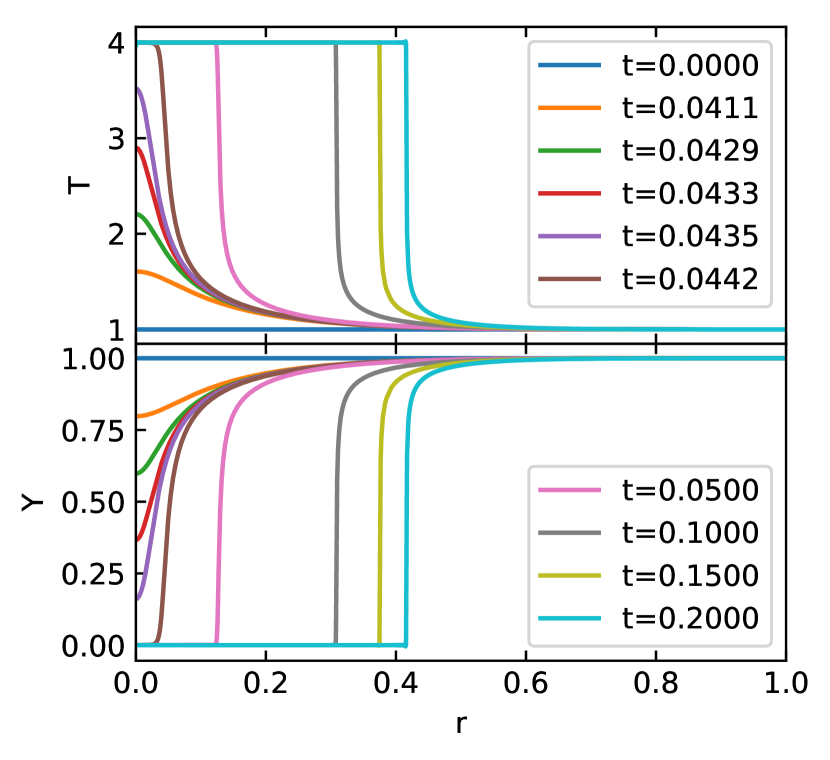
Figure 16: Runaway in the absence of thermal conduction $(K=0)$. The top panel shows the temperature and bottom panel shows the composition. It takes longer for the runaway to complete at larger radii (due to the lower chemical potential), so the region of completion moves outward with time.

As discussed previously, the runaway is seeded on a length scale $l_{\mathrm{runaway}}=\sqrt{1/\Delta_{2}}\approx 0.3$. In the early phase of the runaway the length scale shrinks. As $Y$ is depleted, the reaction rate eventually ceases increasing and begins to decrease. This happens first to parcels in the centre and so the length scale begins to increase as off-centre parcels begin to catch up. This implies there is some minimum length scale, and for the fiducial parameters this is $l_{\mathrm{min}}=0.032$.

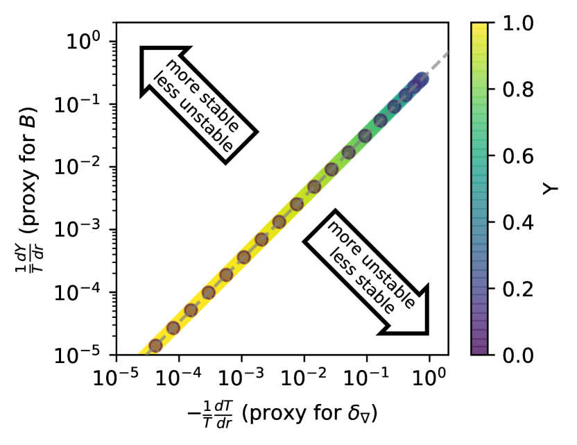
Figure 17: Stability in the absence of thermal conduction ($K=0$). The points show the values in our calculation, regularly spaced in time. The color gives the value of $Y$, as indicated by the color bar. The model begins in the lower left (yellow, $Y=1$) and moves up and to the right as $Y$ decreases. As $Y$ decreases further (dark blue/purple, $Y\la 0.1$), the model reverses and moves back down again towards the lower left. The apparent transition of the points from continuous to discrete as $Y$ decreases is a consequence of the decrease in the time-scale as the runaway proceeds. The grey dashed line shows the analytically expected constant ratio of the T and Y gradients. The arrows indicate the direction in which stability changes; as discussed in the text, we can make only relative statements about stability. If initially stable, this remains stable.

Fig. 17 shows our proxies for $\delta_{\nabla}$ and $B$ as a function of $Y$. Note that this figure and the others like it are log-log plots. Thus a true plot of $\delta_{\nabla}$ vs. $B$ would have the same shape, as the constants of proportionality act as translations. Since $T$ is a linear function of $Y$, the gradients have a constant ratio, $(dT/dr)/(dY/dr)=-q$. This relationship is shown as a grey dashed line and it is clear that it holds at all times during the evolution.

C.2 Infinitesimal diffusion ($K=\epsilon$)

In the presence of an infinitesimally small diffusion coefficient, the temperature evolution of the runaway would remain unchanged. Therefore, we can use the results of the $K=0$ calculation to evaluate the effect of small diffusion coefficients. The sharp temperature gradient at the transition edge leads to heating of the fluid element in advance of the transition, followed by later cooling as it gives the heat back. The change in temperature due to conduction at a location $r$ between the start of the calculation and a time $t$ is given by $K\Theta(r,t)$, where

$$\Theta(r,t)=\int_{0}^{t}\nabla^{2}T(r,t^{\prime})dt^{\prime}~{}.$$ (47)

For values of $t$ in excess of the time it takes the runaway to complete at a location $r$, the value of $\Theta$ will no longer evolve. Fig. 18 shows $\Theta$ at $t=0.05$. The region where the runaway is finished is marked by the bold black line; regions outside of this location are still “active” in terms of heat transfer. Note that in the toy model $r$ is a Lagrangian coordinate.

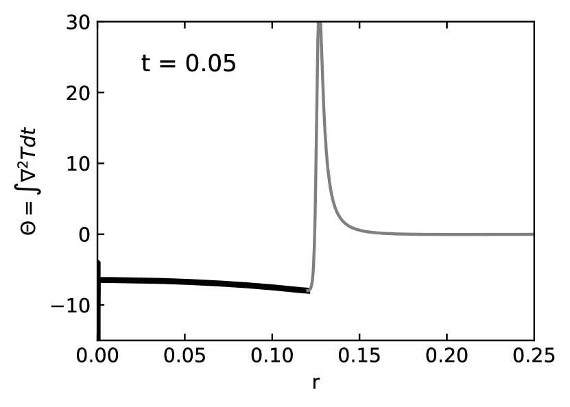
Figure 18: The thick black portion of the line marks where $Y<10^{-4}$. In these regions the runaway is finished and $\Theta$ will no longer evolve with time.

Fig. 18 shows that $\Theta$ is negative near the centre ($r\la 0.1$), indicating that heat is conducted out of the core. More importantly, it shows that $\Theta$ decreases with increasing $r$. This indicates that conduction will cause a residual temperature gradient after the runaway. Taking the time integral (as in equation 47) of all terms in equation (39) gives

$$T(r,t)-1-K\Theta(r,t)=-q\left(1-Y(r,t)\right)$$ (48)

When the runaway has finished, $Y\approx 0$, and this implies that $\frac{dT}{dr}=K\frac{d\Theta}{dr}$ in these regions. Thus, at the end of the runaway, when the composition gradient has vanished, a residual temperature gradient can remain. Fig. 18 indicates that this temperature gradient is radially decreasing and thus has the potential to lead to the onset of convective instability.

C.3 Finite diffusion ($K>0$)

The approximation that thermal diffusion does not affect the runaway must be reasonable only for $K$ less than some value $K_{\mathrm{crit}}$. We now estimate this critical value in two ways. From Fig. 18 we can estimate that the size of the conductive temperature perturbation is $\approx 6K$. Changing the rate given in equation (40) by $e$ requires a temperature change $\approx T^{2}/\Delta_{0}$. For $T\approx 2$ (the geometric mean of the initial and final temperature) this is $\approx 0.6$. Equating these temperature changes suggests a value $K_{\mathrm{crit}}\sim 0.1$. Physically, the characteristic length and time-scales associated with the runaway also give a estimate

$$K_{\mathrm{crit}}\sim\frac{l_{\mathrm{min}}^{2}}{t_{\mathrm{runaway}}}\approx 0.02~{}.$$ (49)

for when conduction will modify the runaway. These estimates agree and so to demonstrate the effects of conduction we solve our toy problem for $K=0.01$ and $K=0.1$.

Fig. 19 shows the $T$ and $Y$ profiles for $K=0.01$. Conduction has not significantly modified the runaway. Fig. 20 shows our stability diagnostic plot for this case. The solution evolves with a constant ratio of $|dT/dr|/|dY/dr|$ (same trajectory as $K=0$), until $Y\ll 1$ at which point this ratio begins to increase. This is evolving in the direction of instability.

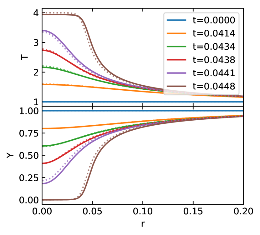
Figure 19: Runaway including thermal conduction for $K<K_{\mathrm{crit}}$ $(K=0.01)$. Same as Fig. 16, but zoomed in on the central region. The dotted lines show the profiles from the model without conduction $(K=0)$ from times with approximately matching central values of $Y$. Conduction has not significantly modified the runaway.

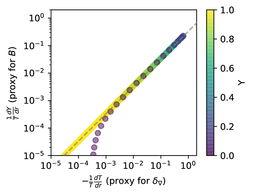
Figure 20: Stability including thermal conduction for $K<K_{\mathrm{crit}}$ $(K=0.01)$, visualized as in Fig. 17. Note that as the Y gradient vanishes, a T gradient remains. Thus even if initially stable, this can evolve to become unstable.

Fig. 21 shows the $T$ and $Y$ profiles for $K=0.1$. Conduction has significantly modified the runaway. Fig. 22 shows our stability diagnostic plot for this case. The solution departs from the $K=0$ trajectory even for $Y\approx 1$, where ratio of $|dT/dr|/|dY/dr|$ decreases, indicating that conduction makes things more stable.

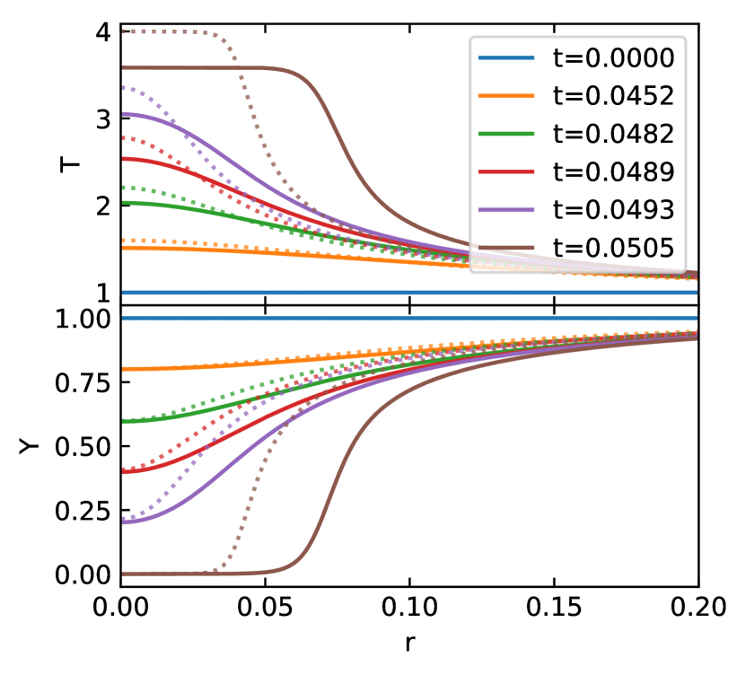
Figure 21: Runaway including thermal conduction for $K\gtrsim K_{\mathrm{crit}}$ $(K=0.1)$. Same as Fig. 16, but zoomed in on the central region. The dotted lines show the profiles from the model without conduction $(K=0)$ from times with approximately matching central values of $Y$. Conduction has significantly modified the runaway.

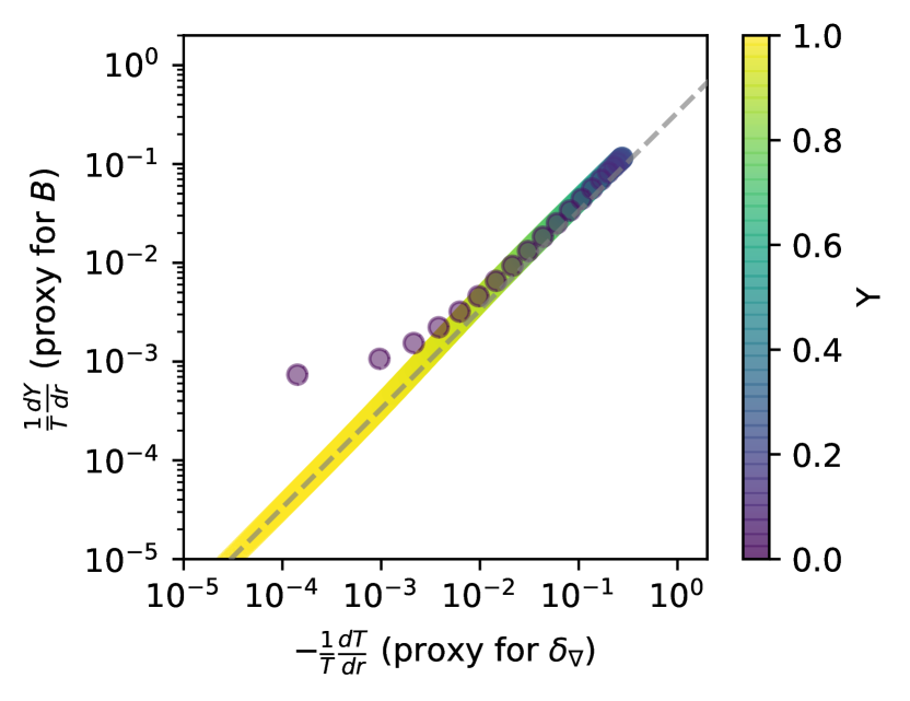
Figure 22: Stability including thermal conduction for $K\gtrsim K_{\mathrm{crit}}$ $(K=0.1)$, visualized as in Fig. 17. The T gradient is always less than it would be in the absence of conduction. Thus if initially stable, this remains stable.

This demonstrates that a thermal runaway driven by sub-threshold electron captures in which thermal conduction operates can lead to convective instability at the centre of a star.

C.4 Connection to MESA Models

In order to complete the connection with our MESA models, we estimate the value of $K$. Since the toy equations are not the same as the equations solved by MESA, this estimate is done at the order of magnitude level. This approximate value $K_{\textsc{MESA}}$ is the appropriately non-dimensionalized version of the thermal diffusivity in the star.

In the dimensionless units associated with the toy problem, we observed the runaway had a minimum length scale of 0.03 and a time scale of 0.05. In the MESA calculation shown in Fig. 9, the runaway has a minimum length scale of $3\times 10^{5}\,\mathrm{cm}$ and a time-scale of $50\,\mathrm{yr}$. That suggests that the time and length scales with which one should non-dimensionalize are $10^{7}\,\mathrm{cm}$ and $10^{3}\,\mathrm{yr}$

The thermal diffusivity at the relevant conditions is $\approx 60\,\mathrm{cm^{2}\,s^{-1}}$. (This is the value returned by the MESA kap module, which uses the results from Cassisi et al. (2007), for $\log(\rho/\mathrm{g\,cm^{-3}})\approx 9.6$ and $\log(T/\mathrm{K})\approx 8.4$ with a 50/50 oxygen-neon mixture.) So we have

$$K_{\textsc{MESA}}\sim\frac{D_{\rm th}}{\rm[L]^{2}/[T]}\sim\frac{60\,\mathrm{cm^{2}\,s^{-1}}}{3\times 10^{3}\,\mathrm{cm^{2}\,s^{-1}}}\sim 0.02~{}.$$ (50)

The range of estimates for $K_{\rm crit}$ found in Section C.3 was 0.02 - 0.1. This indicates that the MESA models are in the regime of finite conductivity, but with $K_{\textsc{MESA}}\la K_{\rm crit}$. Therefore, this toy calculation explains the formation of a central convection zone in our MESA models (see Fig. 8).

Appendix D Comparison with models calculated using tabulated rates

Recently, Suzuki et al. (2016) computed weak reaction rates for the sd-shell nuclei with mass number A=17-28 using the USDB Hamiltonian. They include Coulomb effects and take into account experimentally measured energies and Gamow-Teller transition strengths. These rates are tabulated on a finely-spaced grid of density and temperature. The primary scientific motivation for these new rate tabulations is the evolution of the degenerate oxygen-neon cores that develop in stars with initial masses $\approx 8-10\,\mathrm{\mathrm{M}_{\sun}}$.

We incorporated these rate tables into MESA and used them in place of the on-the-fly rates (described in Section 4.2) to evolve an otherwise identical version of the fiducial model presented in this paper. Fig. 23 compares the central evolution of a model calculated using these tables with our fiducial case. Overall, the agreement is good and there is virtually no variation in the density at oxygen ignition. However, there are small quantitative differences.

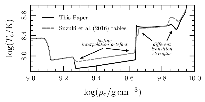
Figure 23: Comparison of the fiducial model presented in this paper with a model evolved using the tabulated weak reaction rates from Suzuki et al. (2016). The models generally agree well. We describe the origin of the indicated differences in the text.

The models agree almost perfectly throughout the $\mathrm{{}^{25}Mg}$-$\mathrm{{}^{25}Na}$ Urca cooling (around $\log(\rho_{\mathrm{c}}/\mathrm{g\,cm^{-3}})\approx 9.1$). This indicates that our on-the-fly rates agree extremely well with the tabulated rates. Differences in the Coulomb corrections would manifest as a shift in density; differences in transition strengths would appear as shifts in temperature. No such differences are seen.

The models begin to disagree near the end of the $\mathrm{{}^{23}Na}$-$\mathrm{{}^{23}Ne}$ Urca cooling (around $\log(\rho_{\mathrm{c}}/\mathrm{g\,cm^{-3}})\approx 9.27$). This reflects the fact that the model has become so cold that even the finely-sampled table of Suzuki et al. (2016) is suffering from the interpolation issues discussed by Fuller et al. (1985) and Toki et al. (2013). The Suzuki et al. (2016) tables are constructed such that these issues do not arise in stars that develop degenerate ONe cores, where the temperatures typically remain $\ga 3\times 10^{8}\,\mathrm{K}$. However, in our more demanding application, we reach temperatures below $10^{8}\,\mathrm{K}$. The extent of the Urca cooling region in density is $\Delta\ln\rho\approx 9(k_{\mathrm{B}}T/E_{\mathrm{F}})$, which is $\approx 0.01$ at these conditions. This is now below the table spacing in this region, which is $\Delta\ln\rho\approx 0.046$. The on-the-fly rates avoid interpolation issues and so our models are more accurate in this regime.

The higher temperature at the end of the $A=23$ Urca cooling leads to the onset of electron captures on $\mathrm{{}^{24}Mg}$ at a slightly lower density. Subsequently, the differences in the two models are primarily due to differences in the assumed strength of the non-unique second forbidden transitions (see Section 5). The $\mathrm{{}^{24}Na}$-$\mathrm{{}^{24}Ne}$ non-unique second forbidden transition is not included in Suzuki et al. (2016); the $\mathrm{{}^{20}Ne}$-$\mathrm{{}^{20}F}$ non-unique second forbidden transition is included at the experimental upper limit. This disagreement is the result of physical ignorance, and so we would not favor one result over the other. One of the motivations for using the on-the-fly rates is the ease with which one can vary experimentally-uncertain transition strengths and thus characterize their effects.

References

- Brooks et al. (2016) Brooks J., Bildsten L., Schwab J., Paxton B., 2016, ApJ, 821, 28
- Brooks et al. (2017) Brooks J., Schwab J., Bildsten L., Quataert E., Paxton B., 2017, ApJ, 834, L9
- Burns et al. (2018) Burns K. J., Vasil G. M., Oishi J. S., Lecoanet D., Brown B. P., Quataert E., 2018, In preparation
- Calaprice & Alburger (1978) Calaprice F. P., Alburger D. E., 1978, Phys. Rev. C, 17, 730
- Canal et al. (1992) Canal R., Isern J., Labay J., 1992, ApJ, 398, L49
- Cassisi et al. (2007) Cassisi S., Potekhin A. Y., Pietrinferni A., Catelan M., Salaris M., 2007, ApJ, 661, 1094
- Chabrier & Potekhin (1998) Chabrier G., Potekhin A. Y., 1998, Phys. Rev. E, 58, 4941
- Denissenkov et al. (2015) Denissenkov P. A., Truran J. W., Herwig F., Jones S., Paxton B., Nomoto K., Suzuki T., Toki H., 2015, MNRAS, 447, 2696
- Farmer et al. (2015) Farmer R., Fields C. E., Timmes F. X., 2015, ApJ, 807, 184
- Firestone (2007a) Firestone R. B., 2007a, Nuclear Data Sheets, 108, 1
- Firestone (2007b) Firestone R. B., 2007b, Nuclear Data Sheets, 108, 2319
- Firestone (2009) Firestone R. B., 2009, Nuclear Data Sheets, 110, 1691
- Fuller et al. (1985) Fuller G. M., Fowler W. A., Newman M. J., 1985, ApJ, 293, 1
- Gamow & Schoenberg (1941) Gamow G., Schoenberg M., 1941, Physical Review, 59, 539
- Gutierrez et al. (1996) Gutierrez J., Garcia-Berro E., Iben Jr. I., Isern J., Labay J., Canal R., 1996, ApJ, 459, 701
- Gutiérrez et al. (2005) Gutiérrez J., Canal R., García-Berro E., 2005, A&A, 435, 231
- Hashimoto et al. (1993) Hashimoto M., Iwamoto K., Nomoto K., 1993, ApJ, 414, L105
- Iben (1978) Iben Jr. I., 1978, ApJ, 219, 213
- Itoh et al. (1996) Itoh N., Hayashi H., Nishikawa A., Kohyama Y., 1996, ApJS, 102, 411
- Jones et al. (2013) Jones S., et al., 2013, ApJ, 772, 150
- Jones et al. (2016) Jones S., Röpke F. K., Pakmor R., Seitenzahl I. R., Ohlmann S. T., Edelmann P. V. F., 2016, A&A, 593, A72
- Kirsebom et al. (2017) Kirsebom O. S., et al., 2017, preprint, (arXiv:1701.01432)
- Lesaffre et al. (2005) Lesaffre P., Podsiadlowski P., Tout C. A., 2005, MNRAS, 356, 131