Analyzing Query Performance and Attributing Blame for Contentions in a Cluster Computing Framework

Abstract

There are many approaches is use today to either prevent or minimize the impact of inter-query interactions on a shared cluster. Despite these measures, performance issues due to concurrent executions of mixed workloads still prevail causing undue waiting times for queries. Analyzing these resource interferences is thus critical in order to answer time sensitive questions like who is causing my query to slowdown in a multi-tenant environment. More importantly, dignosing whether the slowdown of a query is a result of resource contentions caused by other queries or some other external factor can help an admin narrow down the many possibilities of performance degradation. This process of investigating the symptoms of resource contentions and attributing blame to concurrent queries is non-trivial and tedious, and involves hours of manually debugging through a cycle of query interactions.

In this paper, we present ProtoXplore  - a Proto or first system to eXplore contentions, that helps administrators determine whether the blame for resource bottlenecks can be attibuted to concurrent queries, and uses a methodology called Resource Acquire Time Period (RATP) to quantify this blame towards contentious sources accurately. Further, ProtoXplore builds on the theory of explanations and enables a step-wise deep exploration of various levels of performance bottlenecks faced by a query during its execution using a multi-level directed acyclic graph called Proto-Graph. Our experimental evaluation uses ProtoXplore to analyze the interactions between TPC-DS queries on Apache Spark to show how ProtoXplore provides explanations that help in diagnosing contention related issues and better managing a changing mixed workload in a shared cluster.

1 Introduction

There is a growing demand in the industry for autonomous data processing systems [10]. Some critical roadblocks need to be addressed in order to make progress towards achieving the goal of automation. One of these roadblocks is in ensuring predictable query performance in a multi-tenant system. “ Why is my SQL query slow?” This question is nontrivial to answer in many systems. The authors have seen firsthand how enterprises use an army of support staff to solve problem tickets filed by end users whose queries are not performing as they expect. An end user can usually troubleshoot causes of slow performance that arise from her query (e.g., when the query did not use the appropriate index, data skew, change in execution plans, etc.). However, often the root cause of a poorly-performing ‘victim query’ is resource contention caused by some other ‘culprit queries’ in a multi-tenant system [36, 12, 13, 5, 9]. Diagnosing such causes is hard and time consuming. Today, cluster administrators have to manually traverse through such intricate cycles of query interactions to identify how resource interferences can cause performance bottlenecks.

Should the solution be prevention, cure, or both? Features like query isolation at the resource allocation level provide one approach to address the problem of unpredictable query performance caused by contention. For example, an admin tries to reduce conflicts by partitioning resources among tenants using capped capacities [3], reserving shares [17] of the cluster, or dynamically regulating offers to queries based on the configured scheduling policies like FAIR [32] and First-In-First-Out (FIFO). Despite such meticulous measures, providing performance isolation guarantees is still challenging since resources are not governed at a fine-granularity. Moreover, the allocations are primarily based on only a subset of the resources (only CPU in Spark [35], CPU and Memory in Yarn [31]) leaving the requirements for other shared resources unaccounted for. For example, two queries that are promised equal shares of resources get an equal opportunity to launch their tasks in Spark. However, there are no guarantees on the usages of other resources like memory, disk IO, or network bandwidth for competing queries. For instance, if a task uses more resources due to skewed input data on a single host, this can result in higher resource waiting times for tasks of other queries on this host compared to others.

However, in practice, an approach based solely on prevention will not solve the problem. Real-life query workloads are a mix of very diverse types of queries. For example, long-running ETL (Extract-Transform-Load) batch queries often co-exist with short interactive Business Intelligence (BI) queries. Analytical SQL queries are submitted along with machine learning, graph analytics, and data mining queries. It is hard to forecast what the resource usage of any query will be and to control what mix of queries will run at any point of time. In addition, the end users who create and submit the queries may have very different skill levels. All end users may not be skilled enough to submit well-tuned queries. Thus, a practical approach to provide predictable query performance should supplement ‘prevention’ techniques with techniques for ‘diagnosis and cure’.

Our Contributions: This paper focuses on the latter. We present ProtoXplore, - a Proto or first system to eXplore the resource interferences between concurrent queries that provides a framework to attribute blame for contentions systematically. ProtoXplore’s foundations are based on the theory of providing explanations. While there have been several attempts to drill-down to the systemic root causes when a query slows down, we believe that ProtoXplore is a first attempt towards using symptoms of low-level resource contentions to analyze high-level inter-query interactions. Specifically, we make the following contributions: (a) Blame Attribution:  We use the Blocked Times [26] values for multiple resources (CPU, Network, IO, Memory, Scheduling Queue) to develop a metric called Resource Acquire Time Penalty (${\tt RATP}$) that aids us in computing blame towards a concurrent task.(b) Explanations using Proto-Graph:  We present a multi-level Directed Acyclic Graph (DAG), called Proto-Graph, that enables consolidation of ${\tt RATP}$ and blame values at different granularity. (c) Web-based UI for deep exploration:  Our web-based front-end (to be demonstrated in SIGMOD’18 [8]) allows users to explore ProtoXplore and find answers for detecting: (i) hot resources, (ii) slow nodes, (iii) high impact causing culprit queries, and (iv) high impact receiving victim queries..

Our experiments evaluate ProtoXplore using TPCDS queries on Apache Spark. The results of our user-study [1] shows how ProtoXplore helps user of different expertise to reduce debugging effort significantly.

1.1 Related Work

Prevention of Interferences: Approaches like [3, 32] help an admin control resource allocations in a cluster executing mixed workloads. Techniques like resource reservations[17] or dynamic reprovisioning[22] isolate jobs from the effects of performance variability caused by sharing of resources. Our on-going research focuses on prescriptive mechanisms using online explanations generated from ProtoXplore to avoid interferences.

Diagnosis and Cure: Figure 1 presents a summary of how our work compares to the following approaches:

(1) Monitoring Tools: Cluster health monitoring tools like Ganglia [7] and application monitoring tools like Spark UI [11] and Ambari [2] provide an interface to inspect performance of queries.

Table 1: Comparison of ProtoXplore with other approaches

(Category) Related Work	OLAP Workloads	Detect Slow-down	Detect Bottlenecks	Blame Attribution	Data-flow Aware
(1) Ganglia, Spark UI, Ambari	$\checkmark$		$\checkmark$
(2) Starfish, Dr. Elephant, OtterTune	$\checkmark$	$\checkmark$	$\checkmark$
(3) PerfXplain, Blocked Time, PerfAugur	$\checkmark$	$\checkmark$	$\checkmark$
(3) Oracle ADDM, DIADS	$\checkmark$	$\checkmark$	$\checkmark$		$\checkmark$
(4) CPI2		$\checkmark$	$\checkmark^{CPU}$	$\checkmark$
(4) DBSherlock		$\checkmark$	$\checkmark$		$\checkmark$
ProtoXplore	$\checkmark$	$\checkmark$	$\checkmark$	$\checkmark$	$\checkmark$

(2) Configuration recommendation: More recent tools like Starfish[20], Dr.Elephant[6], and OtterTune[30] analyze performance of dataflows and suggest changes in configuration parameters. While these approaches helps in identifying and fixing problems in configurations, it is hard to predict how these system-wide changes will affect the resource interferences from inter-query interactions in an online workload.

(3) Root Cause Diagnosis tools: Performance diagnosis has been studied in the database community [19, 15, 33], for cluster computing frameworks [24, 26], and in cloud based services [27]. The design of ProtoXplore is based on several concepts introduced in these works: (a) Database Community: In ADDM [19], Database Time of a SQL query is used for performing an impact analysis of any resource or activity in the database. ProtoXplore furthers this approach to provide an end-to-end query contention analysis platform while also enabling multi-step deep exploration of contention symptoms. ProtoXplore’s multi-level explanations approach is motivated from DIADS [15]. They use Annotated Plan Graphs that combines the details of database operations and Storage Area Networks (SANs) to provide an integrated performance diagnosis tool. They, however, do not consider any factors related to the impact of these queries in affecting the values of low-level metrics. We believe that this is really important to do an accurate impact analysis. The problem addressed in DIADS is not related, but our multi-level explanation framework bears similarity to their multi-level analysis. Causality based monitoring tools like DBSherlock [33] use causal models to perform a root cause analysis. DBSherlock analyzes performance problems in OLTP workloads, whereas ProtoXplore focuses on performance issues caused by concurrency in data analytical workloads. (b) Cluster Computing: PerfXplain is a debugging toolkit that uses a decision-tree approach to provide explanations for the performance of MapReduce jobs. ProtoXplore  considers dataflow dependencies and workload interactions to generate multi-granularity explanations for a query’s wait-time on resources. Blocked Time metric [26] emphasizes the need for using resource waiting times for performance analysis of data analytical workloads; we use this pedestal to identify the role of concurrent query executions in causing these blocked times for a task. (c) Cloud: PerfAugur [27] identifies systemic causes for query slowdown. Finding the root cause for slowdown is not the focus of ProtoXplore. Our motivation is to enable an admin dignose whether and why this slowdown is a result of resource contentions caused by other queries or some other external factor.

(4) Blame Attribution:
CPI² [36] uses hardware counters for low-level profiling to capture resource usage by antagonist queries while the CPI (CPU Cycles-Per-Instruction) of the victim query takes a hit. Since this approach does not capture multi-resource contentions at application-level, it suffers from finding poor correlations when queries impact on other resources. Blame attribution has also been studied in the context of program actions [18]. The purpose and application addressed in ProtoXplore is totally different.

(5) Other work on explanations in databases: The field of explanations has been studied in many different contexts like data provenance [16], causality and responsibility [25], explaining outliers and unexpected query answers [32, 28], etc. The problem studied and the methods applied in this paper are unrelated to these approaches.

Roadmap.  In Section 2 we describe the key challenges in analyzing dataflows, multi-resource contentions and attributing blame in a shared cluster. We present our blame attribution process in Section 4. We describe the construction of Proto-Graph in Section 6. Our experimental and user-study results are in Section 8, and finally conclude with on-going and future work in Section 9.

2 Challenges

In this section, we review some challenges for blame attribution and discuss the motivation behind our work.

Figure 1: Dataflow DAG of an example query $Q_{0}$.

Example

Consider the dataflow DAG of a query $Q_{0}$ in Figure 1 comprising stages $s_{0},s_{1},\cdots,s_{5}$. The stage $s_{5}$ is the final or root stage, whereas the leaves $s_{0},s_{1},s_{2}$ scan input data. The stage $s_{3}$ can start only when all of $s_{0},s_{1},s_{2}$ are completed. Suppose an admin notices slowdown of a recurring query $Q_{0}$ shown in Figure 1 in an execution compared to a previous one, and wants to analyze the contentions that caused this slowdown. The admin can use tools like SparkUI [11] to detect that tasks of stage $s_{1}$ took much longer than the median task runtime on host (i.e., machine) $X$, and then can use logs from tools like Ganglia [7] to see that host $X$ had a high memory contention. Similarly she notices that $s_{5}$ was running on host $Y$ that had a high IO contention. Further, the admin sees that stage $r_{3}$ of another query $Q_{1}$ was executing concurrently with only stage $s_{5}$ of $Q_{0}$, while stages $u_{5},u_{7},u_{9}$ of query $Q_{2}$ were concurrent with both $s_{1}$ and $s_{5}$.

Challenge 1. Assessing Performance bottlenecks:
Use of blocked time [26] alone to compare impact due to resource contentions can be misleading.

Suppose both the target stages $s_{1}$ and $s_{5}$ spent the same time waiting for a resource (say, CPU); the impact of contention faced by them could still differ if they processed different sizes of input data. Identifying such disproportionality in wait-times can help an admin diagnose victim stages in a dataflow .

Challenge 2. Capturing Resource Utilizations:
Low-level resource usage trends captured using hardware counters cannot be used towards blame attribution for queries.

Approaches like capturing the OS level resource utilizations [36] require computing the precise acquisition and release timeline of each resource using hardware counters, and associating them with the high-level abstract task entities. This is non-trivial especially for resources like network (as requests are issued in multiple threads in background) and IO (requests are pipelined by the OS).

Figure 2: Example overlap of resource usage between $Task_{1}$ and $Task_{2}$. Notice the multiplexing between the tasks for compute time.

Challenge 3. Capturing Resource Interferences:
CPU Time stolen from concurrent queries is inadequate to capture multi-resource contentions.

As shown in Figure  2, tasks can use and be also blocked on multiple resources simultaneously [26] resulting in multi-resource interferences between concurrent tasks. As a result, metrics like stolen time [9] cannot be used as is to quantify blame as it is used only in the context of identifying processes that steal CPU time. Capturing time stolen for multiple resources simultaneously requires a more involved metric for blame attribution.

Challenge 4. Avoiding False Attributions:
Overlap Time between tasks of a query does not necessarily signal a contention for resources between them.

Today, admins consider only the % overlap between concurrent queries to assign blame, which may lead to faulty attributions. For example, even if stage $s_{5}$ of $Q_{0}$ had total overlap with IO-intensive tasks of $Q_{2}$, this contention may not have impacted $s_{5}$ owing to its minimal IO activity (later stages in data analytical queries typically process less data).

Challenge 5. Analyzing Contentions on Dataflows:
Dataflow dependencies and parallel stage executions make it harder to diagnose the root cause of overall query slowdown.

In the above example, stages $s_{1}$ and $s_{5}$ of $Q_{0}$ (in dark red) were a victim of contention, but there is no easy way for the admin to know which of these stage of $Q_{0}$ was responsible in its overall slowdown. Additionally, diagnosing whether $Q_{1}$ or $Q_{2}$ (and which of their stages) is primarily responsible for creating this contention is hard.

Motivation: There are several intricate possibilities even in this toy example, whereas there may be long chains of stages running in parallel in a real production environment making this process challenging. Today admins have limited means to analyze the impact due to query-interactions apart from looking at individual cluster utilization logs, specific query logs, and manually identifying correlations in both. This forms the motivation of our work.

3 System Overview

ProtoXplore is a system that helps us address the above challenges using our methodology for blame attribution and our graph-based model used for consolidation of blame. It enabes users to detect contentions online while the queries are executing, or perform a deep exploration of contentious scenarios in the cluster offline. Figure 3 shows an overview of ProtoXplore’s architecture.

Figure 3: ProtoXplore System Architecture

In Step (1), an admin uses tools like Spark UI [11] to monitor the execution of queries and then identifies a set of queries to be analyzed. Target query and target stages: Any query in the system can be a potential source or a target of contention. Each of the queries chosen for deep exploration in ProtoXplore is termed as a target query $Q_{t}$, its stages as target stages, and its tasks as target tasks. ProtoXplore currently provides an interface to analyze contentions faced by (i) all stages in the longest path of execution, (ii) any single stage, and (iii) all stages in the target query(our default option).

Source query and source stages: We refer to other concurrently running queries $Q_{s}$ that can possibly cause contention to a target query $Q_{t}$ as source queries (if the stage(s) of $Q_{s}$ are waiting in the scheduler queue or running concurrently with the stage(s) of $Q_{t}$). Stages of $Q_{s}$ are source stage, and its tasks are source tasks. Finally, we refer to source queries that cause multi-resource contentions for several concurrent queries with high impact as aggressive queries.

Once the user submits target queries to ProtoXplore in step (3), the Proto-Graph Graph Constructor builds a multi-level graph as described in Section 6 for these queries (Step (4)). In addition, users can configure the resources or hosts for which they want to analyze the contentions. For example, users can diagnose impact of concurrency on only scheduler queue contentions, or CPU contention on a subset of hosts, or source queries submitted by a particular user etc. For each task of a target stage, ProtoXplore computes the RATP and blame metrics as described in Section 4. The Blame Attributor module then consolidates these values for stages, as shown in Step (5), which are then used to update the node and edge weights of the graph subsequently. The Explanations Generator updates a degree of responsibility (DOR) metric for each node, which is then used by the Blame Analysis API to generate explanations at various granularities (step (6)). Specifically, we generate three levels of explanations for a query’s slowdown due to resource interferences, namely Immediate Explanations (IE), Deep Explanations (DE), and Blame Explanations (BE) that lets users identify sources of contentions at resource, host and query levels respectively. These explanations are then consumed in Step (7) by the Rule Generator to output heuristics for the admin (like alternate query placement, dynamic priority readjustment for stages and queries). The details of rule generation is out of scope of this paper and is focus of our ongoing research; a preliminary implementation with basic rules can be found in the demo paper [8]. In step (8), these rules are stored for the admin to later review and apply to the cluster scheduler. The web-based interface presents a dashboard to the admin to visualize cluster and query performance statistics, contention summary graphs for a selected workload, hints in selection of target queries for analysis, top-k sources of impact to the selected target queries, and the corresponding Proto-Graph [8]. Next, we discuss the theory behind our Blame Attributor module.

4 Blame Attribution

In order to address the challenges 1-4 described in Section 2, we develop a metric called Resource Acquire Time Penalty (RATP) that helps us formulate the blame towards concurrent tasks.

4.1 Resource Acquire Time Penalty (RATP)

In a $\delta\tau$ interval, let the time spent by a target task $tt$ to acquire ${\tt RA}_{tt,r,h}^{\delta\tau}$ units of resource $r$ on host $h$ be:

$$T_{tt,r,h}^{\delta\tau}={\tt WT}_{tt,r,h}^{\delta\tau}+{\tt CT}_{tt,r,h}^{\delta\tau}$$ (1)

where, ${\tt WT}_{tt,r,h}^{\delta\tau}$ is the time spent blocked or waiting for the resource and ${\tt CT}_{tt}^{\delta\tau}$ is the time spent consuming it in this interval. For the remaining section, we assume that the resource $r$ and host $h$ are fixed, so we omit $r,h$ in the subscripts and other places for simplicity where it is clear from the context.

Definition

We define the Resource Acquire Time Penalty (RATP) for $tt$ for resource $r$ on host $h$ in interval $\delta\tau$ as:

$$RATP_{tt}^{\delta\tau}=\frac{\left({\tt WT}_{tt}^{\delta\tau}+{\tt CT}_{tt}^{\delta\tau}\right)}{{\tt RA}_{tt}^{\delta\tau}}$$ (2)

4.2 Slowdown of a task

In the $\delta\tau$ interval, let the capacity of a host $h$ to serve a resource $r$ be $\mathcal{C}$ units/sec (note: $r,h$ superscripts omitted). Thus, the total used capacity by all consumers of resource $r$ is bounded by the system capacity $\mathcal{C}$, expressed as:

$$\mathcal{C}=\mathcal{C}_{tt}+\mathcal{C}_{1}+\mathcal{C}_{2}+\dots+\mathcal{C}_{n}+\sum_{1}^{k}\mathcal{C}_{ki}+\sum_{1}^{l}\mathcal{C}_{ui}\vspace{-1mm}$$ (3)

where, $\mathcal{C}_{tt}$ is the capacity used by target task $tt$; $\mathcal{C}_{1},\mathcal{C}_{2},\dots\ \mathcal{C}_{n}$ are the individual used capacities by $n$ other concurrent tasks; whereas $\mathcal{C}_{ki}$ and $\mathcal{C}_{ui}$ represents capacities used by other $k$ known and $l$ unknown causes. The minimum time required to acquire resource $r$ on this host can then be expressed as ${\tt RATP}^{\delta\tau}=\frac{1}{C}$ sec/unit. Thus, slowdown of task $tt$ due to unavailability of resources is:

Definition

Slowdown $\mathcal{S}_{tt}$ of a task $tt$ in interval $\delta\tau$ between time $\tau$ and $\tau+\delta\tau$ is defined as

$$\mathcal{S}_{tt}^{\delta\tau}=\frac{({\tt RATP}_{tt}^{\delta\tau}-{\tt RATP}^{\delta\tau})}{{\tt RATP}^{\delta\tau}}$$ (4)

where, ${\tt RATP}_{tt}^{\delta\tau}$ is computed as per Equation  2.

Intuitively, it is the deviation from the ideal resource acquire time on that host. Therefore, the slowdown corresponds to the blame that can be attributed to unavailability of resources which can be attributed to other tasks running concurrently with $tt$ on $h$ during its execution, or on other quantities as shown in Equation 3, giving us:

$$\mathcal{S}_{tt}^{\delta\tau}=\underbrace{(\sum_{1}^{n}\beta_{st\rightarrow tt}^{\delta\tau})}_{p_{1}}+\underbrace{\sum_{1}^{k}\beta_{ki\rightarrow tt}^{\delta\tau}+\sum_{1}^{l}\beta_{ui\rightarrow tt}^{\delta\tau}}_{p_{2}}\vspace{-5.5mm}$$ (5)

Here $\beta_{ss\rightarrow ts}^{\delta\tau}$ is the blame assigned to each of the $n$ concurrent tasks executing on the same host during task $tt$’s execution. Wait-times for resources are sometimes also due to processes that are part of the framework but not a valid symptom of interferences between tasks. (e.g., garbage collection for CPU, HDFS replication for network). These processes impact all concurrent tasks alike for the specific resource. $\beta_{ki\rightarrow tt}^{\delta\tau}$ gives the blame value assigned to other known non-concurrency related causes that result in task $tt$’s wait-time. Finally, slowdown could be due to a variety of other causes which are either not known or cannot be attributed to any concurrent tasks. $\beta_{ui\rightarrow tt}^{\delta\tau}$ captures this value of slowdown due to systemic issues.

4.3 Slowdown due to Concurrency

The slowdown defined in $p_{2}$ of Equation 5 is the best case slowdown for using resource $r$ on host $h$ in the absence of any interferences due to concurrency. We now derive $p_{1}$ of Equation 5. First we discuss a simpler case, when there is a full overlap of $tt$ with concurrently running tasks to present the main ideas. Then we discuss the general case with arbitrary overlap between $st$ and $tt$.

4.3.1 Full overlap of $tt$ with concurrent tasks

Rewriting Equation (3) using ${\tt RATP}$ values to account for capacities used by running tasks (omitting the known and unknown causes) in interval $\delta\tau$:

$$\frac{1}{{\tt RATP}^{\delta\tau}}=\frac{1}{{\tt RATP}_{tt}^{\delta\tau}}+\frac{1}{{\tt RATP}_{1}^{\delta\tau}}+\frac{1}{{\tt RATP}_{2}^{\delta\tau}}+\dots+\frac{1}{{\tt RATP}_{n}^{\delta\tau}}$$

$$\frac{{\tt RATP}_{tt}^{\delta\tau}-{\tt RATP}^{\delta\tau}}{{\tt RATP}^{\delta\tau}}=\frac{{\tt RATP}_{tt}^{\delta\tau}}{{\tt RATP}_{1}^{\delta\tau}}+\dots+\frac{{\tt RATP}_{tt}^{\delta\tau}}{{\tt RATP}_{n}^{\delta\tau}}$$

$$\mathcal{S}_{tt}^{\delta\tau}=\left[\sum_{st\in\ n}\frac{{\tt RATP}_{tt}^{\delta\tau}}{{\tt RATP}_{st}^{\delta\tau}}\right]$$ (6)

Each term on the right hand side of the above equation is contributed by one of the source tasks concurrent to task $tt$, and corresponds to blame attributable to a source task $st$ in this interval, that is, $\beta_{st\rightarrow tt}^{\tau}=\frac{{\tt RATP}_{tt}^{\tau}}{{\tt RATP}_{st}^{\tau}}$.

4.3.2 Partial overlap with concurrent tasks

The above derivation works for a time interval in which all concurrent tasks have a total overlap with $tt$. In practice, they overlap for different length of intervals as can be seen from Figure 4. As a result, we cannot use Equation (6) directly to attribute blame to a source task $st$. To derive blame for this scenario, we divide the total duration $T=tt_{end}-tt_{start}$ of task $tt$’s execution time in $\delta\tau$ intervals such that in each $\delta\tau$ time-frame the above Equation (6) holds.

Let $\mathcal{S}_{1},\mathcal{S}_{2},\dots\ ,\mathcal{S}_{m}$ be the slowdown in each of the $m=\frac{T}{\delta\tau}$ intervals of the task’s execution. This gives us the mean slowdown of $tt$ as ($T_{tt}$ is the execution time of $tt$):

$$\mathcal{S}_{mean}=\frac{\delta\tau}{T_{tt}}\sum_{k\in m}\mathcal{S}_{k}$$

$$\mathcal{S}_{mean}=\frac{\delta\tau}{T_{tt}}\sum_{k\in m}\sum_{st\in\theta_{k}}\frac{{\tt RATP}_{tt}^{k}}{{\tt RATP}_{st}^{k}}$$

$$\mathcal{S}_{mean}=\sum_{st\in\theta}\sum_{k\in m^{\prime}}\frac{{\tt RATP}_{tt}^{k}}{{\tt RATP}_{st}^{k}}\frac{\delta\tau}{T_{tt}}$$

The above equation in the limiting case is:

$$\mathcal{S}_{mean}=\sum_{st\in\theta}\left[\int_{o^{start}_{st,tt}}^{o^{end}_{st,tt}}\frac{{\tt RATP}_{tt}}{{\tt RATP}_{st}}\frac{dt}{T_{tt}}\right]$$ (8)

where, $o^{end}_{st,tt}$ - $o^{start}_{st,tt}$ is the overlap time between tasks ${tt}$ and ${st}$. The integral inside the summation is the total blame towards a source task $st$, giving us the definition of blame:

Figure 4: An example overlap between concurrent tasks.

Proposition

The blame $\beta_{ss\rightarrow tt}^{\delta\tau}$ for the contention caused by a task $st$ of a source query to the task $tt$ of a target query on host $h$ for resource $r$ in interval $\tau$ to $\tau+\delta\tau$ can be expressed as

$$\beta_{st\rightarrow tt}^{\delta\tau}=\frac{1}{T_{tt}}\left[\int_{o_{st,tt}^{start}}^{o_{st,tt}^{end}}\frac{{\tt RATP}_{tt}^{\delta\tau}}{{\tt RATP}_{st}^{\delta\tau}}d\delta\tau\right]$$ (9)

where, $o_{st,tt}^{end},o_{st,tt}^{start}$ denote the ending and starting points of the overlap time between tasks $tt$ and $st$ (on host $h$), and $T_{tt}$ is the total execution time of task $tt$.

5 Implementation

In this section, we discuss how we derive blame in practice, the supported resources for analyzing blame, and the metrics support we have instrumented in Spark.

5.1 Blame Formulation using Blocked Time

A task continues to execute even when its resource request is not completely fulfilled (especially for IO and Network) [26]. This is because these resources are pipelined to it by background application threads or by the OS. Hence a source task’s real impact (attributable blame) is only to the extent that the target task is blocked for the resource. This adjustment is also important to predict the expected speed up of target task more accurately. If an admin decides to kill a source task because of its contention then he can only expect an improvement proportional to target task’s blocked time (not its entire resource acquision time). The blocked time ${\tt WT}_{tt,r,h}^{\delta\tau}$ values (see Equation 1) are also relatively more easier to capture as shown in  [26]. We thus define an adjusted RATP for a task $tt$ as:

$${\tt RATP}\textit{-blocked }_{tt}^{\delta\tau}=\frac{{\tt WT}_{tt}^{\delta\tau}}{{\tt RA}_{tt}^{\delta\tau}}$$ (10)

For the source task though, we continue to use the entire interval $\delta\tau$ as time spent to acquire ${\tt RA}_{st}^{\delta\tau}$ units of resource instead of its blocked time. This lowers the attributable blame further but allows us to account for those sources whose blocked time may not be available (especially terms of $p_{2}$ in Equation  5) For clarity, we represent this as max RATP which for a source $st$ is as:

$${\tt RATP}\textit{-max }_{st}^{\delta\tau}=\frac{\delta\tau}{{\tt RA}_{st}^{\delta\tau}}$$ (11)

The blame value we use is therefore:

$$\beta\textit{-blocked }_{st\rightarrow tt}^{\delta\tau}=\frac{1}{T_{tt}}\left[\int_{o_{st,tt}^{start}}^{o_{st,tt}^{end}}\frac{{\tt RATP}\textit{-blocked }_{tt}^{\delta\tau}}{{\tt RATP}\textit{-max }_{st}^{\delta\tau}}d\delta\tau\right]$$ (12)

As blocked time in an interval is bound by the total interval length, $\beta\textit{-blocked }_{st\rightarrow tt}^{\delta\tau}\leq\beta_{st\rightarrow tt}^{\delta\tau}$.

5.2 Handling Known Causes:

A query may experience slowdown due to myriad reasons like systemic issues (executors getting killed, external processes, etc), the query’s own code (used the wrong index, change in query plan, etc.) and many more. The wait-time for every resource can be attributed to any of these issues besides concurrency. On the other hand, concurrenct executions may have additional indirect consequences like slowdown of a task due to increase in garbage collection time owing to a previously executed resource-intensive task, etc. Research in the area of diagnosing such known and unknown systemic causes for performance degradation is well established [24, 33, 21], which is out of the scope of discussion of this paper. Although ProtoXplore’s primary focus is to account for the $\beta_{st\rightarrow tt}^{\delta\tau}$ term, it also comes pre-configured for attributing blame to select known causes like JVMGCTime (cpu), HDFS repartitioning (IO) and RDD storage (Memory) etc. ProtoXplore also allows adding known causes via its feedback module where users with domain knowledge and prior experience with ProtoXplore can configure support for them. ProtoXplore also avoids false attribution by using catch-all term for unknown causes as we show next.

5.3 Avoiding False Attributions:

Our quantification of blame $\beta\textit{-blocked }_{st\rightarrow tt}$ enables us to distinguish between legitimate and false sources of contention owing to the following characteristics: (i) Since the blame is computed only for periods where $tt$ is blocked for resource $r$ during the overlap period, the blame on $st$ is zero if $tt$’s wait-time is zero during the overlap. (ii) If both $st$ and $tt$ are not waiting for the same resource in the overlapping time (see Challenge 2), $st$ does not qualify for blame. Blame attribution using mere overlap time can miss this subtlety. (iii) Finally, slowdown could be due to a variety of other causes which are either not known or cannot be attributed to any concurrent tasks. To handle these cases, ProtoXplore creates a synthetic unknown source query in the framework. We assume that such a query overlaps with all tasks of every query on every host of execution. For every resource, we then keep a track of the system-level resource used values (currently ProtoXplore is configured for IO bytes read/written and network bytes read resources) during each execution window. We compute the total-unaccountable-resource by subtracting the resource acquired values for all tasks running during that window from the system-level metric. The blame attributed to this unknown source is then computed by using the ${\tt RA}_{st}^{\delta\tau}=\textit{total-unaccountable-resource}$ in the ${\tt RATP}\textit{-max }_{st}^{\delta\tau}$ computation of Equation 12.

5.4 Supported Resources

The values of resource acquired ${\tt RA}_{tt}^{\delta\tau}$ for most resources like input or output bytes, shuffle bytes read, etc., and some wait-time metrics like fetch-wait-time, shuffle-write-time and scan-time for a task are available through Spark’s default metrics. For additional metrics (denoted with a superscript ^∗ against them) and time-series data we added instrumentation to Spark and built per-host agents (for system metrics). In each window of data collected during task $tt$’s execution, we consider contention for the following resources on host $h$:

• Network: We compute ${\tt RATP}_{network}$ using the Network Wait Time (NWT) or fetch-wait-time metric from Spark. The value of resource acquired ${\tt RA}_{network}$ is the shuffle bytes read metric in that window.

• Memory: To capture the contention for process-managed memory , we compute (i) ${\tt RATP}_{storage-mem}$ using storage memory wait time (${\tt SMWT}^{*}$) and storage memory acquired^∗, (ii) ${\tt RATP}_{exec-mem}$ using execution memory wait time (${\tt EMWT}^{*}$) and execution memory acquired^∗ metrics.

• IO: We compute the RATP for IO Read ${\tt RATP}_{io-read}$ using scan-time and bytes read in the scan operation. For IO Write, its ${\tt RATP}_{io-write}$ is given using shuffle-write-time and shuffle-bytes-written metrics in Spark.

• CPU: Apart from above resources, a task’s execution can wait due to other reasons like os scheduling wait ,acquiring locks/monitors, priority lowering etc. We capture (a) monitor and lock wait time metrics from JMX (b) garbage collection wait time from spark existing metrics and (c) attribute all other wait time to os scheduling delay. We deal with garbage collection specially by creating a synthetic GC query in our model as a possible source of contention. This query is modeled to have a single long running task on each executor. This task is assumed to block all other tasks during the duration of its execution. We also attribute the remaining unaccounted wait time in an interval to the OS scheduling wait time. As the blame due to a concurrent task is based on ${\tt RATP}$ ratios, any error in this way of accounting for scheduling wait is minimized to a large extent. Finally for each of the above CPU-impacting wait-times, we use the value of executor-cpu-time as the resource acquired.

5.5 Frequency of Metrics Collection:

For each task $tt$, we added support to collect the timeseries data for its wait-time and the corresponding data processed metrics at the boundaries of task start and finish for all other tasks $st$ concurrent to $tt$. Figure 5 shows the four cases of task start end boundaries concurrent to target task $tt$. That is, instead of collecting the timeseries data at regular $\delta\tau$ intervals as shown in Figure 4, we capture it only for concurrency related events that can have an impact on a task’s RATP values. Note that with this approach, the extent of each $\delta\tau$ depends on the frequency of arrival and exit of concurrent tasks, thus enabling us to capture the effects of concurrency on a task’s execution more accurately.

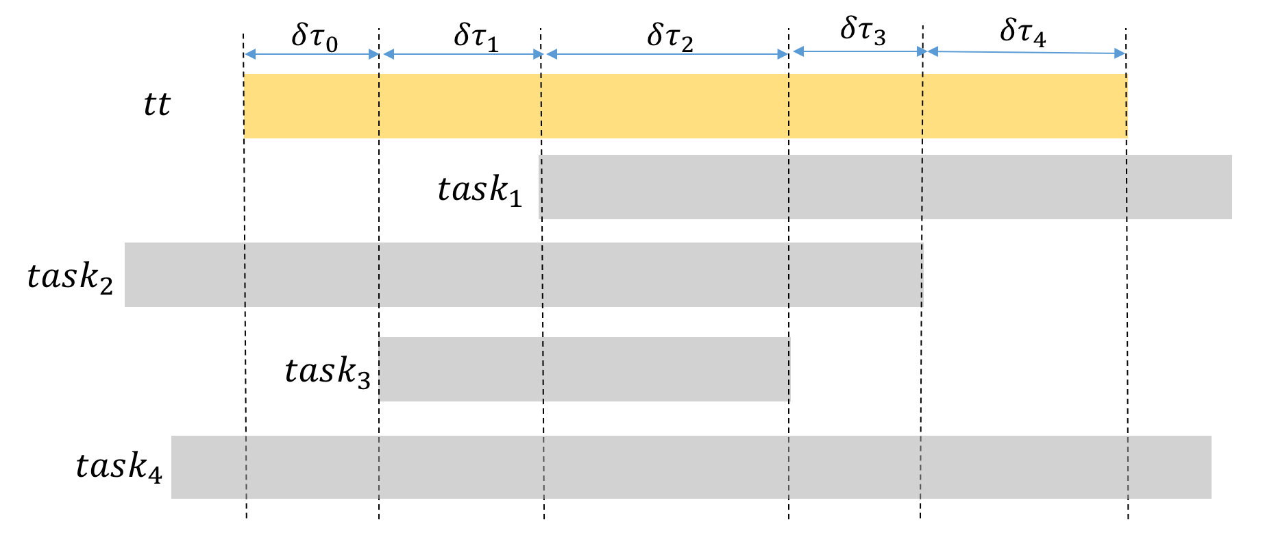
Figure 5: We collect metrics data at concurrent task start and end boundaries.

However, if the arrival rate of concurrent tasks is low, this can affect the distributions of our metric values. To address this, we also record the metrics at heartbeat intervals in addition to above task entry and exit boundaries. On the other hand, for workloads consisting of tasks with sub-second latency, our approach gives more fine-grained windows for analysis. Section 8 compares the impact of both the approaches on the quality of our explanations.

6 iQC-Graph

In the previous section, we discussed our methodology to assign blame towards a concurrent task $st$ for causing contention to a target task $tt$. As seen previously, a query typically consists of a dataflow of stages where each stage is composed of multiple parallel tasks. In order to consolidate blame caused or faced by a query, we construct Proto-Graph, a multi-layered directed acyclic graph.

6.1 Levels in Proto-Graph

We now describe the levels in Proto-Graph (the full pseudo-code for constructing it can be found in [23] due to space constraints). Level 0 and Level 1 contain the target queries and target stages respectively – these are the queries or stages that the admin wants to analyze. On the other end of Proto-Graph, Level 6 represents all source queries, while Level 5 contains all source stages, which are the queries and stages concurrently running with the target queries. Note that it is important to separate the queries and their stages in two different levels at both ends of Proto-Graph- this is to diagnose impacts from and to multiple stages of a query.

The middle three levels – Levels 2, 3 and 4 (described shortly) – keep track of causes of contentions of different forms and granularity that enable us to connect these two ends of Proto-Graph with appropriate attribution of responsibility to all intermediate nodes and edges. Levels 2, 3, and 4 answer the impact questions described above respectively.

6.2 Vertex Contributions

For each node $u$ in the graph, we assign weights, called Vertex Contributions denoted by ${\tt VC}_{u}$, that are used later for analyzing impact and generating explanations. Specifically, ${\tt VC}_{u}$ measures the standalone impact of $u$ toward the contention faced by any target query vertex in Level-0. The VC values of different nodes are carefully computed at different levels by taking into account the semantics of respective nodes. For Level 0 target query, Level 5 source stage, and Level 6 source query vertices, we currently set ${\tt VC}_{u}=1$ for all nodes $u$ in each level. Our admin interface allows to configure these based on the requirements of the workload, e.g. assign higher weights to queries from certain users, or SLA-driven queries. For the Level 1 target stage vertices, we set this to the cumulative CPU time (i.e., the work done) by stage $s$ in order to assign higher impacts through stages that get more work done. We now describe Levels 2-4, and show how we compute these values for them.

Level 2 - Track Resource Level Contentions: For each target stage in Level 1, we add five nodes in Level 2 corresponding to each of the resources, namely scheduling slots, CPU, network, IO and memory. From Equation 2, the ${\tt RATP}$ of a task $tt$ for resource $r$ during its execution from time $t_{start}$ to $t_{end}$ (integrate over all $\delta\tau$ intervals) on host $h$ (superscripts $r,h$ ommitted) is:

$$\vspace{-2mm}{\tt RATP}_{tt}=\int_{\tau_{tt}^{start}}^{\tau_{tt}^{end}}{\tt RATP}_{tt}^{\delta\tau}d\delta\tau$$ (13)

For each node $u$ in Level-2, we assign its $VC_{u}^{\ell_{2}}$ to be the cumulative ${\tt RATP}$ for all tasks of this target stage vertex in Level-1 as:

$${\tt VC}_{u}^{\ell_{2}}=\sum_{tt}\int_{\tau_{tt}^{start}}^{\tau_{tt}^{end}}{\tt RATP}_{tt}^{\tau,r,h}d\delta\tau$$ (14)

Level 3 - Track Host Level Contentions: Level-3 unfolds the components of wait time distribution of a target stage further to keep track of the ${\tt RATP}\textit{-blocked}$ values of each stage for a specific resource on each host of its execution. First, we find all the hosts that were used to execute the tasks of a particular target stage. Then, for everynode in Level 2 corresponding to resource $r$, we add $P_{r}\times H$ new nodes in Level 3, where $P_{r}$ is the number of different requests that can lead to a wait time for resource $r$, and $H$ is the number of hosts involved in the execution of this target stage. For instance, the IO bottleneck of a target stage can be explained by the distribution of time spent waiting for ${\scriptsize\tt IO\_READ}$ and ${\scriptsize\tt IO\_WRITE}$. Therefore, for $r$ = IO, $P_{r}=2$, and for each host we add two nodes for IO_BYTES_READ_RATP and IO_BYTES_WRITE_RATP in Level 3. The Level-3 nodes for other resources are generated as discussed in Section 5.4.

The value of ${\tt VC}_{u}^{\ell_{3}}$ is set similar to Equation 14 except that the summation is done over all tasks of a target stage (denoted as $h-tasks$) executing only on host $h$ in question.

$${\tt VC}_{u}^{\ell_{3}}=\sum_{tt\in h-tasks}\int_{\tau_{tt}^{start}}^{\tau_{tt}^{end}}{\tt RATP}_{tt}^{\tau,r,h}d\delta\tau$$ (15)

Level 4 - Linking Cause to Effect: For each node $v$ in Level 3 corresponding to a target stage, host $h$, and type of resource request $r$, if the tasks of this target stage were executing concurrently with tasks belonging to $P$ distinct source stages on host $h$, we add $P$ nodes $u$ in Level 4 and connect them to $v$. The ${\tt VC}_{u}^{\ell_{4}}$ of each node is then computed from the blame attribution of all target stages in Level 3 that it can potentially affect.

$${\tt VC}_{u}^{\ell_{4}}=\sum_{tt\in h-tasks}\beta\textit{-blocked }_{st\rightarrow tt}^{r,h}$$ (16)

6.3 iQC-Graph by example

In example  2, suppose the user selects $Q_{0}$ as the target query, and wants to analyze the contention of the stages on the critical path. First, we add a node for $Q_{0}$ in Level 0, and nodes for $s_{1},s_{3},s_{4},s_{5}$ in Level 1. Then in Level 2, for each of these stages, the admin can see five nodes corresponding to different resources. Although both $s_{1}$ and $s_{5}$ faced high contentions, using Proto-Graph the admin can understand questions such as whether the network contention faced by stage $s_{5}$ was higher than the IO contention faced by stage $s_{1}$, and so on.

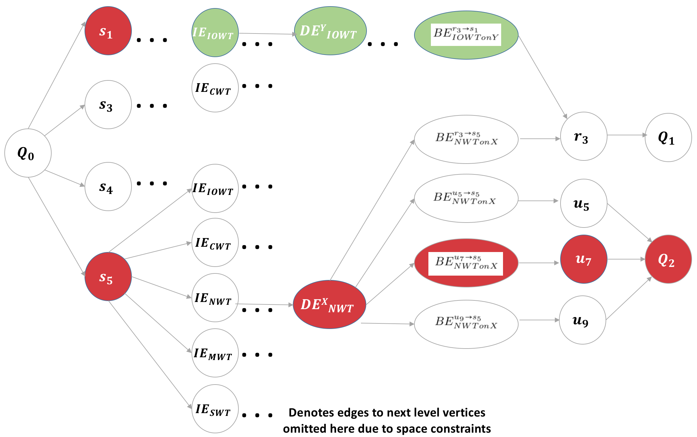
Figure 6: Proto-Graph illustrating the details in Example 6.3

Suppose only the trailing tasks of stage $s_{1}$ executing on host $Y$ faced IO contention due to data skew. Using Proto-Graph, a deep explanation tells the user that IO_BYTES_READ_RATP on host $Y$ for these tasks of $s_{1}$ was much less compared to the average RATP for tasks of stage $s_{1}$ executing on other hosts. This insight tells the user that the slowdown on host $Y$ for tasks of $s_{1}$ was not an issue due to IO contention. If the user lists the top-$k$ nodes at Level-3 using our blame analysis API, she can see that the network RATP for tasks of stage $s_{5}$ on host $X$ was the highest, and can further explore the Level-4 nodes to find the source of this disproportionality.

Since stage $r_{3}$ of source query $Q_{1}$, and stages $u_{5},u_{7},u_{9}$ of another source query $Q_{2}$ were executing concurrently on host $X$ with stage $s_{5}$ of $Q_{0}$, the user lists the top-$k$ Level-4 vertices responsible for this network contention for $s_{5}$. The blame analysis API outputs stage $u_{7}$ of query $Q_{2}$ as the top source of contention. Figure 6 shows some relevant vertices for this example to help illustrate the levels in Proto-Graph.

Discussion: Note that we consider the cumulative RATP values for computing stage-level values (in Equation 14 and Equation 15). The other alternative approaches include considering max or average values for the tasks in a stage; however, sum captures the total cluster time (similar to the notion of Database Time in [19]) spent on waiting for resources per unit data by each stage and, thus, enables us to analyze the overall slowdown of a stage in the cluster.

7 Explanations

In this section, we describe how the choice of a graph-based model enables us to consolidate the contention and blame values for generating explanations for a query’s peformance.

7.1 Generating Explanations

The Explanations Generator module in ProtoXplore uses the VC values to update two metrics, namely Impact Factor (IF) and Degree of Responsibility (DOR). We set the IF as edge weights and DOR as the node properties.

Impact Factor (IF): Once the Vertex Contributions ${\tt VC}_{u}$ of every node $u$ in Proto-Graph is computed to estimate the standalone impact of $u$ on a target stage, we compute the Impact Factor ${\tt IF}_{uv}$ on the edges $(u,v)$. This enables us to distribute the overall impact received by each child node $v$ among its parent nodes $u$-s. For instance, ${\tt IF}_{uv}$ from a DE node $u$ to an IE node $v$ gives what fraction of total impact on an IE node can be attributed to each of its parent DE nodes. Figure 7 shows an example of the impact received by node $u_{1}$ from nodes $v_{1},v_{2},v_{3}$.

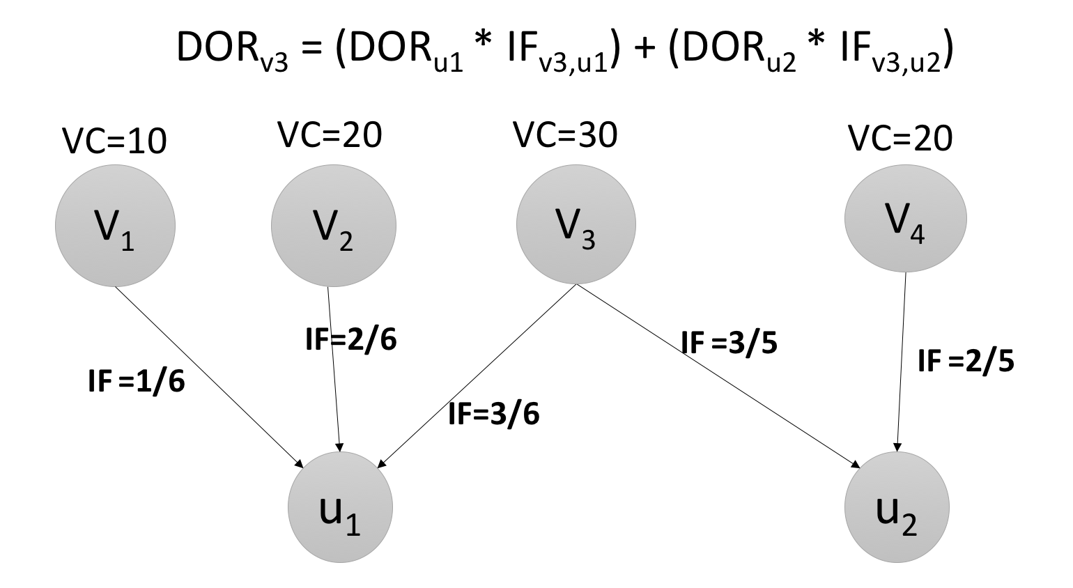
Figure 7: Example computation of DOR from IF and VC values.

The IF values of the edge weights are used to generate explanations as follows:

An explanation in ProtoXplore takes the form:
Expl($~{}{\tt tq},~{}{\tt ts},~{}{\tt res},~{}{\tt res^{\prime}},~{}{\tt host},~{}{\tt ss},~{}{\tt sq},~{}{\mathcal{P}}$)
where ,
tq denotes the target stage being explained by ${\phi}$; ts denotes the target stage being explained by ${\phi}$; res $\in{CPU,Memory,IO,Network,Scheduling}$; res’ is the type of resource impacted (see Section 5.4); host is the host of impact; ss is the stage of the concurrent query that has caused impact; sq is the impacting source query; ${\mathcal{P}}$ is the cumulative weight of the path originating from sq and ending at tq.

7.2 Contention Analysis using iQC-Graph

A top-$k$ analysis lets user specify the number of top explanations she is interested in. Additionally, ProtoXplore consolidates the explanations further to aggregate responsibility of each entity (queries, stages, resources and hosts) towards the contention faced by every target query.

Degree of Responsibility (DOR): Finally we compute the Degree of Responsibility ${\tt DOR}_{u}$ of each node $u$, which stores the cumulative impact of $u$ on a target query $t$. The value of ${\tt DOR}_{u}$ is computed as the sum of the weights of all paths from any node $u$ to the target query node $t$, where the weight of a path is the product of all ${\tt IF}_{vw}$ values of all the edges $(v,w)$ on this path. If we choose more than one query at Level 0 for analysis, a mapping of the values of DOR toward each query is stored on nodes at Level 5 and 6. The computation of DOR of node $v_{3}$ is illustrated in Figure  7. It can be noted that since our framework incorporates impacts originating from the synthetic ‘Unknown’ source, it enables an admin to rule out slowdown due to concurrency issues if the impact through this nodes is high. Using DOR, users can perform the following use-cases that enable deep exploration of contentions in a shared cluster:

• Finding Top-K Contentions for Target Queries: For any query in the workload, users can find answers for: (a) What is the impact through each resource for its slowdown? (b) What is the impact through each host for a specific resource? and, (c) What is the impact through each source query or source stage on a specific host and resource combination?

• Detecting Aggressive Source Queries: ProtoXplore allows the admin to do a top-down analysis on a source query or source stage to explore how it has caused high impact to all concurrent queries. To detect such aggressive queries, we find the (top-$k$) Level 6 nodes having the highest value of total DOR toward all affected queries (recall that for each source query, we keep track of the DOR value toward each target query).

• Identifying Slow Nodes and Hot Resources: Performing a top-$k$ analysis on levels 2 (resources) and 3 (hosts) will yield the hot resource and its corresponding slow node with respect to a particular target query. In order to get the overall impact of each resource or each host on all target queries, ProtoXplore provides an API to (i) detect slow nodes, i.e., group all nodes in Level 3 by hosts, and then output the total outgoing impact (sum of all IF values) per host, and (ii) detect hot resources, i.e., - output the total outgoing impact per wait-time component nodes in Level 2.

8 Evaluation

Our experiments were conducted on Apache Spark 2.2 [35] deployed on a 20-node local cluster (master and 19 slaves). Spark was setup to run using the standalone scheduler in FAIR scheduling mode [34] with default configurations. Each machine in the cluster has 8 cores, 16GB RAM, and 1 TB storage. A 300 GB TPC-DS [14] dataset was stored in HDFS and accessed through Apache Hive in Parquet [4] format. The SQLs for the TPC-DS queries were taken from the implementations in [29] without any modifications.

Workload: Our analysis uses a TPCDS benchmark workload that models multiple users running a mix of data analytical queries in parallel. We have 6 users (or tenants) submitting their queries to their dedicated queue. Each user runs queries sequentially from a series of randomly chosen 15 TPCDS queries. When submitting to a queue, the selection of queries is randomized for each user. The query schedules were serialized and re-used for each of our experiments to enable us to compare and contrast results across executions. During the experiments, our cluster slots were 97% utilized and Ganglia showed around 36% average CPU utilization.

We now describe how ProtoXplore enables deeper diagnosis of contentions compared to (a) Blocked-Time Analysis (BTA): we use the values of blocked times for IO and Network [26] and aggregate them at stage and query levels, (b) Naive-Overlap: based on overlap times of query runtimes (a technique popularly used by support staff trying to resolve who is affecting my query tickets), and (c) Deep-Overlap: we compute the cumulative overlap time between all tasks of a pair of concurrent queries.

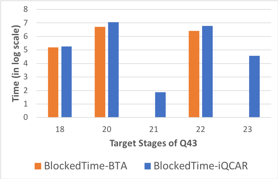
(a)

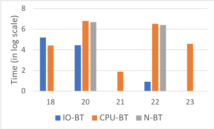
(b)

Figure 8: (a) Resource blocked times from ProtoXplore and BTA approach; (b) Blocked times for IO, CPU and Network.

8.1 Comparison with Baseline

For this experiment, we identify a target query $Q_{43}$ from our workload that was 178% slower compared to its unconstrained execution (when run in isolation). Figure 8(a) compares the bottlenecks observed (y-axis is on log scale) with the BTA method vs the blocked times captured by ProtoXplore for its impacted stages (other stages had minimal blocked times to compare). In addition to the blocked times from network and IO, ProtoXplore accrues additional blocked times that help to identify potential causes of slowdown for stages like 21 and 23. Figure 8(b) compares the relative per resource blocked times. The network and CPU blocked time is significantly high for stages 20 and 22. However, when we compare the RATP’s for these stages using ProtoXplore, we see in Figure 9(a) that the CPU RATP was much higher for multiple stages compared to their IO RATP, whereas the network RATP was significantly low to even compare. If we analyze the impact on each of these stages generated using the explanations module, stage 20 received the maximum impact through CPU compared to others. This detailed analysis cannot be obtained from looking at BTA alone.

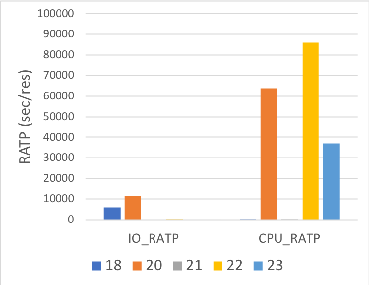
(a)

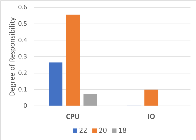
(b)

Figure 9: (a) RATP for IO and CPU for high-impacting stages, and (b) their DOR in impacting $Q_{43}$.

Next, for assessing who is causing the above slowdown to $Q_{43}$, we compare our results with Naive-Overlap and Deep-Overlap. For the overlap-based approaches, highest blame is attributed to query with most overlap. It can be seen from Figure 10 that the top queries that overlap differ significantly between Naive-Overlap and Deep-Overlap. The queries with minimal overlap shown in Naive-Overlap ($Q_{4}$ and $Q_{27}$) have relatively more tasks executing in parallel on the same host as that of target query, causing higher cumulative Deep-Overlap. The output from ProtoXplore is more comparable to Deep-Overlap, but has different contributions. Especially for $Q_{11}$, where the tasks had a high overlap with tasks of our target query $Q_{43}$, the impact paths showed low path weights between these end points. A further exploration revealed that only 18% of the execution windows (captured via the time-series metrics), showed increments in CPU and IO acquired values for $Q_{11}$ for the matching overlapping windows. $Q_{11}$ itself was blocked for these resources in 64% of the overlapping windows. Without the impact analysis API of ProtoXplore, an admin will need significant effort to unravel this.

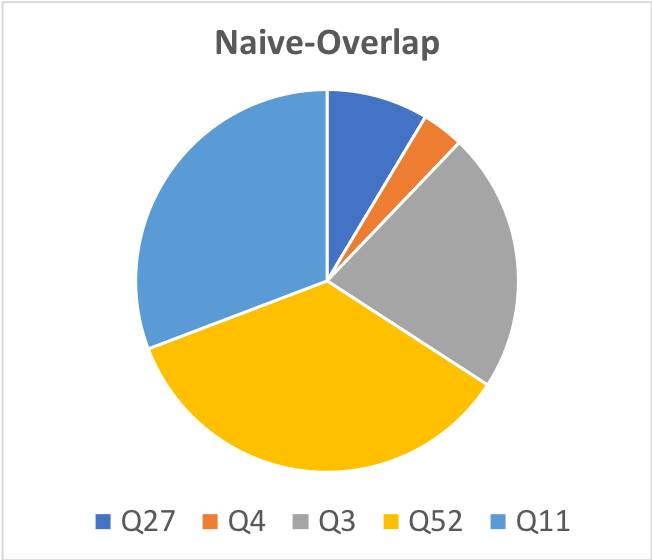
(a)

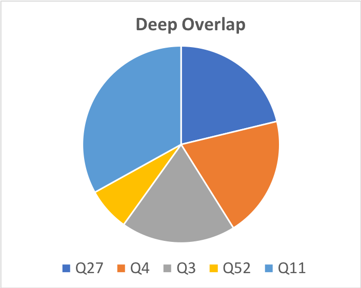
(b)

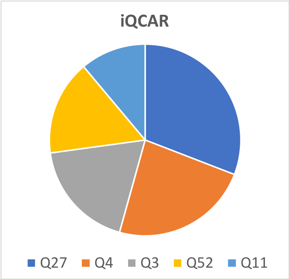
(c)

Figure 10: Compare top-$5$ impacting queries between (a) Naive-Overlap (b) Deep-Overlap and (c) ProtoXplore.

8.2 Test Cases

The purpose of our second set of experiments is three-fold to: (i) verify that ProtoXplore detects symptoms of contentions induced in our workload and outputs newly identified sources, (ii) demonstrate how ProtoXplore achieves this for a running workload, and (iii) how we can perform a time-series analysis with ProtoXplore. Our test-cases for induced resource contention scenarios are summarized in Table 2. ProtoXplore detects contentions for Spark’s managed memory, hence the test-case of Memory-external is out of scope. Note, we were not able to isolate contention only due to increased shuffle data as it was always resulting in increasd IO contention too owing to shuffle write. So induction of network contention in our workload (sql queries) was not possible. We now share our induction methodology and observations:

Table 2: Summary of Induced Contention Scenarios

Test-Case	Detail
CPU-Internal	User-7 submits a CPU-intensive custom SparkSQL query just after $Q_{43}$ starts.
CPU-External	We inject a CPU-intensive custom query in a seperate Spark application instance.
IO-Internal	User-7 submits a IO-intensive custom SparkSQL query at a random time.
IO-External	A large 60GB file is read in 256MB block size on every host just after $Q_{43}$ starts.
Memory-Internal	User-7 caches web_sales table just before $Q_{43}$ starts.

8.2.1 CPU-Internal

For this experiment, we use the same workload as before (the schedules were serialized), and induce contention query $Q_{cpu-int}$ shown in Listing 1 along with our target query $Q_{43}$. This query $Q_{cpu-int}$ exhibits the following characteristics: (a) low-overhead of IO read owing to a scan over two small TPCDS customer tables each containing 5 million records stored in parquet format, (b) low network overhead since we project only two columns, (c) minimal data skew between partitions as the join is on c_customer_sk column which is a unique sequential id for every row and shuffle operation used hash-partitioning , and (d) high CPU requirements owing to the sha2 function on a long string (generated by using the repeat function on a string column). We now analyze the contentions of target query $Q_{43}$ further. Note that our induction can affect $Q_{43}$ only to a certain extent owing to multiple aspects of scheduling on a cluster, for example the concurrency of tasks of $Q_{cpu-int}$ with tasks of $Q_{43}$ is dependent on the number of slots it can get under the configured scheduling policy. Despite this, ProtoXplore is able to capture $Q_{cpu-int}$ as one of the top sources in the concerned window as we show next.

Listing 1: $Q_{cpu-int}$: CPU-Internal Induction query

⬇

with temp

(select c1.c_first_name as first_name,

sum(sha2(

repeat(c1.c_last_name,

45000),512)) as shasum

from customer c1,customer c2

where c1.c_customer_sk

= c2.c_customer_sk

group by c1.c_first_name)

select max(shasum)

from temp

limit 100;

Observations: Figure 11 shows that the CPU utilization reaches almost 80% during our induction, much higher than the 36% average utilization for our workload.

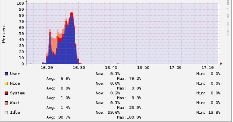
Figure 11: Ganglia snapshot showing CPU Utilization when $Q_{cpu-int}$ was running.

Figure 12 shows the change in DOR values of the source queries towards $Q_{43}$. The live analysis windows cpu_live_1, cpu_live_2, cpu_live_3 and cpu_live_total show the periods in which we invoke ProtoXplore to analyze contentions on $Q_{43}$. The stacked bars show the relative contribution from each of the top-$5$ running sources, and their heights denote the total contribution from these five sources. Since we are analyzing contentions on only $Q_{43}$, the cpu_live_1 window shows no contributions as $Q_{43}$ had not started yet. $Q_{cpu-int}$ was induced at the end of window cpu_live_2, hence no contribution from $Q_{cpu-int}$ in this window. However, as seen in cpu_live_3, once we induce $Q_{cpu-int}$ when $Q_{43}$ starts, its contribution of 27% is detected.

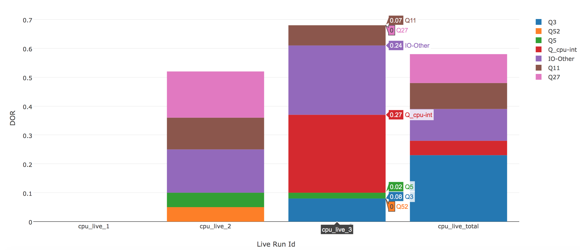
Figure 12: DOR of $Q_{cpu-int}$ is about 27% towards query $Q_{43}$ during CPU induction.

The end-of-window analysis in cpu_live_total shows the overall impact $Q_{43}$ from all sources during its execution. Although $Q_{cpu-int}$ caused high contention to $Q_{43}$ for a period, its overall impact was still limited ($0.05\%$). Details like this are missed by alternative approaches like Naive-Overlap) and Deep-Overlap as shown in Figure 13. Moreover, an analysis with even Deep-Overlap can mislead the user into attributing about 35% of received impact to $Q_{11}$, whereas, the actual impact output by ProtoXplore shows less than 1% overall impact from $Q_{11}$.

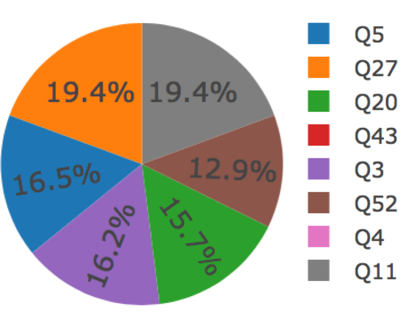
(a) Naive Overlap

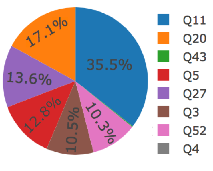
(b) Deep Overlap

Figure 13: Impact from source queries.

8.2.2 IO-External

To induce IO outside of Spark, we read and dump a large file on every host in the cluster after the workload stabilizes (at least one query is completed for each user). Let us call this query as $IO-Other$. The timing of induction was chosen such that it overlaps with the scan stage of $Q_{43}$. We created a 60GB file on each host and used the command in 2 to read in blocks of size 256MB using the below command:

Listing 2: $IO-Other$: IO-External Induction query

⬇

dd if=~/file_60GB of=/dev/null bs=256

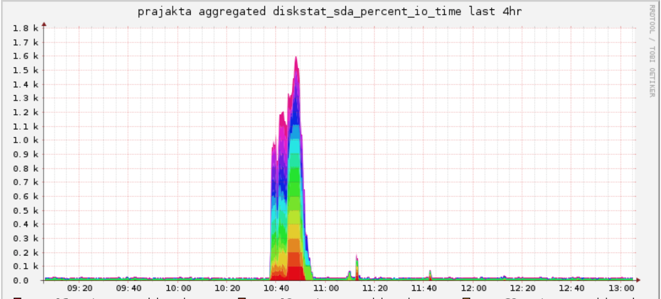
Figure 14: Ganglia snapshot showing aggregate IO utilization during our external induction.

Observations: Figure 14 shows over 1600% aggregate disk utilization for all nodes (19 slaves) in the cluster during this period of contention. We analyze impacts from sources for the following windows: (a) $Q_{43}$ had not started in io_live_1, (b) io_live_2 analysis was done for target query $Q_{43}$ just before we induced $IO-Other$, (c) io_live_3 to io_live_5 windows while $IO-Other$ is running concurrently with $Q_{43}$ (we omit showing io_live_4 due to plotting space constraints), (d) $Q_{43}$ finishes execution before io_live_6 ,and (e) the io_live_total window to analyze overall impact on $Q_{43}$ from the beginning of the workload till the end. Figure 15 shows the relative contributions from each of the concurrent sources, showing that ProtoXplore detects the induced contention first in io_live_3 (shown in green), and outputs an increasing impact during io_live_4 and io_live_5 when it peaks.

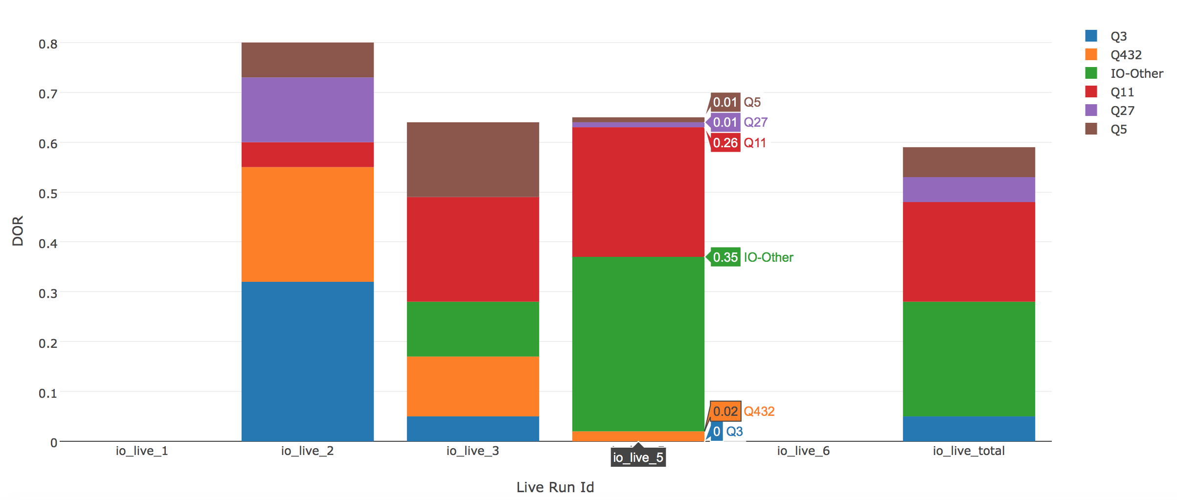
Figure 15: DOR of source queries towards query $Q_{43}$ changes as the workload progresses.

8.2.3 Mem-Internal

Since we monitor contention only for the managed memory within Spark, our internal memory-contention test-case caches a large TPCDS table (web_sales) in memory just before $Q_{43}$ is submitted. Let’s call this query as $Q_{mem-int}$.

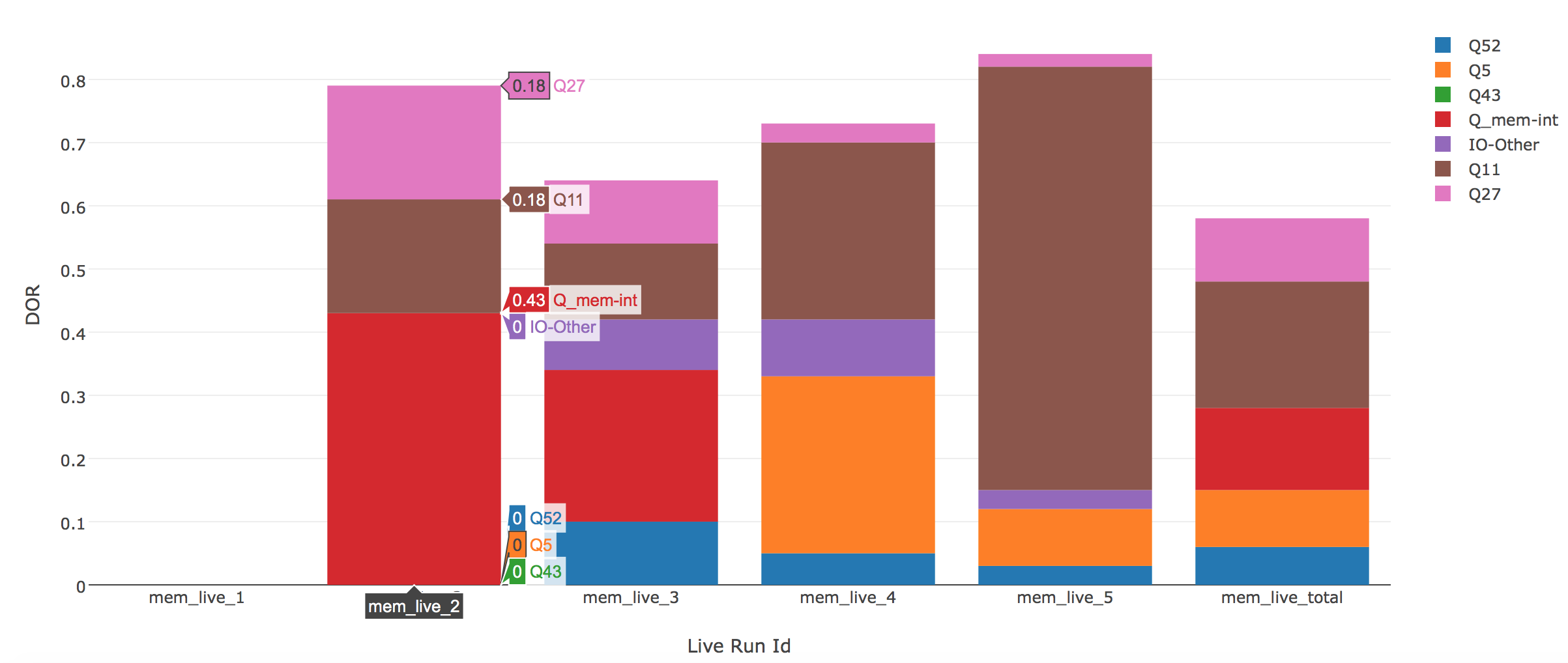
Figure 16: Impact of induced internal memory contention on $Q_{43}$.

Observations: We now analyze the impact on $Q_{43}$ for the following four windows: (a) mem_live_2 is the period where both $Q_{43}$ and $Q_{mem-int}$ had begun execution together ($Q_{43}$ had not started in mem_live_1), (b) mem_live_3 shows a window where some other queries had entered the workload, and both $Q_{43}$ and $Q_{mem-int}$ were still running, (c) mem_live_4 and mem_live_5 are the windows when $Q_{43}$ was still running and $Q_{mem-int}$ had finished execution, and (d) mem_live_total analyzes the overall impact on $Q_{43}$ from top-$5$ sources during its complete execution window. While $Q_{43}$ was running concurrently with multiple other queries, $Q_{mem-int}$ causes more than 40% share of the total impact received once it begins as shown in Figure 16. Note that $Q_{43}$ scans store and store_sales, whereas we cached web_sales in our induction query.

8.3 Frequency of Data Collection

In this experiment, we analyze the impact of varying the frequency of collecting time-series data on the quality of our explanations (i.e.DOR values of the sources) towards a target query’s performance. Figure 17 shows that as the intervals reduce from 10s-2s, the accuracy of the DOR values for all queries (calculated using vector distance) improves and approaches to our ideal case of $TE$ (task-event and 2s interval collection). This value is highly sensitive to the task median runtimes of the workload. For example, a 8s heartbeat time-series collection can miss the impacts on 6s tasks. Our task-event metrics collection approach, thus, enables ProtoXplore to generate more accurate blames. We next discuss the overheads associated with this instrumentation.

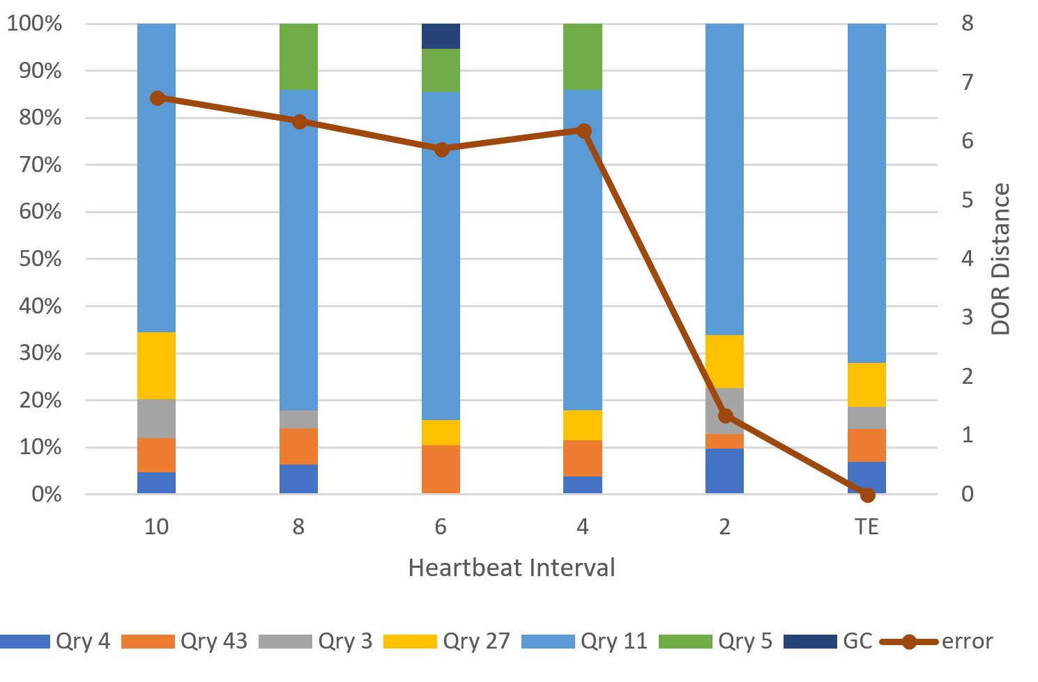
Figure 17: Impact of varying intervals of metrics collection on explanation DORs. ($TE$ denotes the metrics collection at task-event boundaries (Section 5.5) in addition to 2s logging.

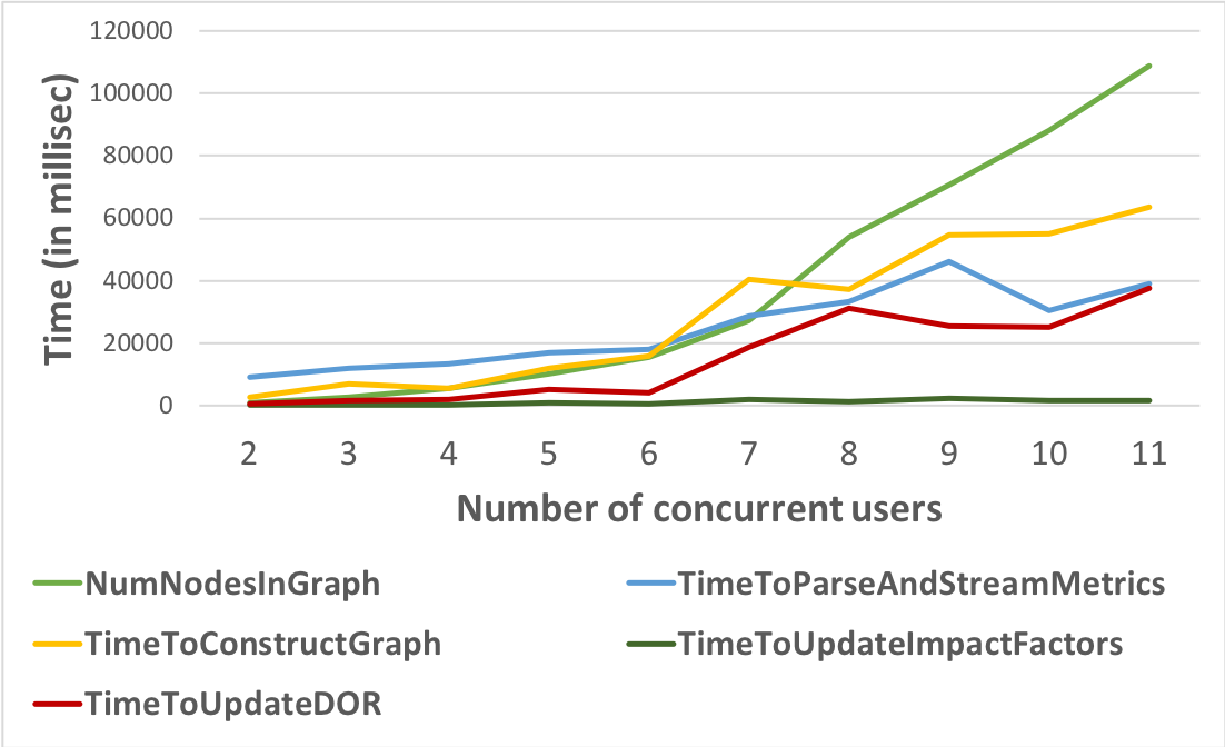
(a)

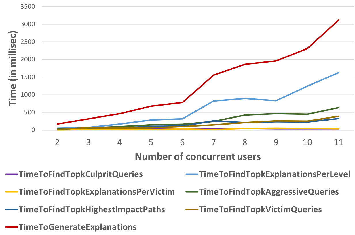
(b)

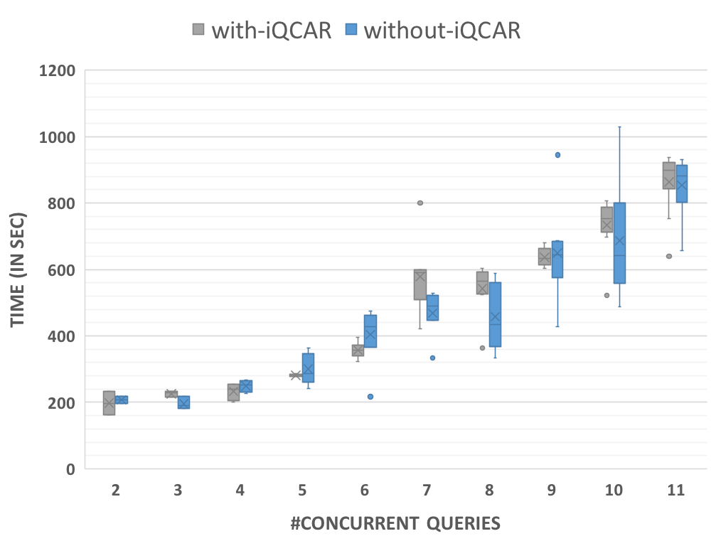
(c)

Figure 18: Time taken by the Graph Constructor (Part (a)) and the Explanations Generator (part (b)) modules in various steps. Part (c) shows the overhead of our instrumentation on the runtime of queries in the workload.

8.4 Instrumentation

Figure 18(c) compares the runtime of our workload in Spark with (grey) and without (blue) our instrumentation for publishing time-series for the metrics listed in Section 5.4. The heartbeat was set to 2s and task-event metrics collection was set to true - a scenario of maximum load that our instrumentation can put.

Since every node in Levels 2, 3 and 4 corresponds to a particular target stage, the subgraph formed by these nodes for one target stage at Level 1 is disjoint from the subgraph formed by the nodes for another target stage. They are connected back at Level 5 if multiple target stages execute concurrently with the same source stage. This property enables us to construct the subgraphs from Level 0 to Level 4 in parallel. Figure 18(a) shows the time taken in parsing time-series data and creating our data model, constructing graph, and times to update the edge weights (IF) and node weights (DOR). Figure 18(b) presents the times spent for different types of analysis algorithms. From our experience, the runtime of this Graph Constructor module dominates the overall latency of outputting explanations in ProtoXplore.

User-Study	Novice		Skilled		Expert
	M	P	M	P	M	P
Easy	28	80	0	100	0	75
Medium	14	40	0	66	16	60
Hard	16	70	0	66	33	66

Table 3: Percent correct answers - Manual (M) vs ProtoXplore (P)

8.5 User Study

We performed a user study involving participation from users with varying levels of expertise in databases, Spark and in using system monitoring tools like Ganglia. Briefly, we categorize our users based on their combined experience in all three of these categories as (a) Novice (e.g. undergrad or masters database student or users with $\leq$ 1 yr experience), (b) Skilled (e.g. industry professionals with 1-3 yrs experience) and (c) Expert (e.g. DB researcher or industry professionals with more than 3 yrs experience). As such, we had 4 Experts, 2 Skilled and 4 Novice users. This web-based tool enabled the users to analyze a pre-executed micro-benchmark to answer an online questionnaire consisting of 10 multiple-choice questions with mixed difficulty levels. We categorized our questions as Easy, Medium and Hard based on the number of steps involved and the time it took to answer them manually by one of our Experts. At the beginning of study, each user was randomly assigned 5 questions to be answered with manual analysis using existing monitoring tools [11, 7]. The users were then shown the ProtoXplore user-interface (UI) to answer the rest of the 5 questions. Each question was presented progressively and the time taken to answer it was recorded in order to distinguish between genuine and casual participants. Note that in the ProtoXplore UI, we purposefully refrained from showing the users the final answers generated by ProtoXplore; instead, we presented them with plots based on (a) the measured wait-time and data processed values and (b) consolidated DOR values at each level that aided the users in selecting their answers using ProtoXplore tool. This activity enabled us to match the answers generated from ProtoXplore with those selected by our Expert users with manual analysis.

In total, users attempted 54% of our questions requiring manual analysis since they gave up on the remaining questions, whereas they answered 98% of the questions using ProtoXplore interface. They got 37% answers correct with manual analysis, and 69% right using ProtoXplore. Table  3 summarizes the results based on levels of expertise. It shows that using only visual aids on impact values and resource-to-host RATP heatmaps, the accuracy of selecting correct answers increased for each type of user compared to manual analysis. One interesting observation from our user-study is that once the users were finally given an opportunity to compare and review their chosen answers with those generated by ProtoXplore supplemented with a reasoning, they agreed to accept the output generated by ProtoXplore for 90% of the mis-matched answers. In our results, the time taken by the users in answering the questions manually was about 19% lesser than the time they took to answer using ProtoXplore UI. When we explored further to understand this counter-intuitive result, we noticed that irrespective of user expertise, most of them spent significant time in answering the first one or two questions but then gave up on the answers too easily for later questions. Whereas, they spent time in exploring the ProtoXplore UI to attempt more answers.

9 Conclusion

Resource Interferences due to concurrent executions are one of the primary and yet highly mis-diagnosed causes of query slowdowns in shared clusters today. This paper discusses some challenges in detecting accurate causes of contentions, and illustrates with examples why blame attribution using existing methodologies can be inaccurate. To this effect, we propose a theory for quantifying blame for slowdown, and present techniques to filter genuine concurrency related slowdowns from other known and unknown issues. We further showed how our graph-based framework allows for consolidation of blame and generate explanations allowing an admin to explore the contentions and contributors of these contentions systematically.

References

- [1] A User Study for Evaluating ProtoXplore. http://152.3.145.69:9007/protoXploreFE/.
- [2] Apache Ambari. http://ambari.apache.org.
- [3] Apache Hadoop Capacity Scheduler. http://hadoop.apache.org/docs/current/hadoop-yarn/hadoop-yarn-site/CapacityScheduler.html.
- [4] Apache Parquet. https://parquet.apache.org.
- [5] Collection of small tips in further analyzing your hadoop cluster. https://www.slideshare.net/Hadoop_Summit/t-325p210-cnoguchi.
- [6] Dr. Elephant. http://www.teradata.com.
- [7] Ganglia Monitoring System. http://ganglia.info.
- [8] iQCAR: A Demonstration of an Inter-Query Contention Analyzer for Cluster Computing Frameworks. https://users.cs.duke.edu/~sudeepa/SIGMOD2018-iQCAR-demo.pdf.
- [9] Netflix and Stolen Time. https://www.sciencelogic.com/blog/netflix-steals-time-in-the-cloud-and-from-users.
- [10] Oracle Autonomous Database. https://www.oracle.com/database/autonomous-database/index.html.
- [11] Spark Monitoring and Instrumentation. http://spark.apache.org/docs/latest/monitoring.html.
- [12] The Noisy Neighbor Problem. https://www.liquidweb.com/blog/why-aws-is-bad-for-small-organizations-and-users/.
- [13] Understanding AWS stolen CPU and how it affects your apps. https://www.datadoghq.com/blog/understanding-aws-stolen-cpu-and-how-it-affects-your-apps/.
- [14] TPC Benchmark™DS . http://www.tpc.org/tpcds/, 2016. [Online; accessed 01-Nov-2016].
- [15] N. Borisov, S. Babu, S. Uttamchandani, R. Routray, and A. Singh. Why did my query slow down? arXiv preprint arXiv:0907.3183, 2009.
- [16] P. Buneman, S. Khanna, and W. C. Tan. Why and where: A characterization of data provenance. In Proceedings of the 8th International Conference on Database Theory, pages 316–330, 2001.
- [17] C. Curino, D. E. Difallah, C. Douglas, S. Krishnan, R. Ramakrishnan, and S. Rao. Reservation-based scheduling: If you’re late don’t blame us! In Proceedings of the ACM Symposium on Cloud Computing, pages 1–14. ACM, 2014.
- [18] A. Datta, D. Garg, D. Kaynar, D. Sharma, and A. Sinha. Program actions as actual causes: A building block for accountability. In 2015 IEEE 28th Computer Security Foundations Symposium, pages 261–275. IEEE, 2015.
- [19] K. Dias, M. Ramacher, U. Shaft, V. Venkataramani, and G. Wood. Automatic performance diagnosis and tuning in oracle. In CIDR, pages 84–94, 2005.
- [20] H. Herodotou, H. Lim, G. Luo, N. Borisov, L. Dong, F. B. Cetin, and S. Babu. Starfish: a self-tuning system for big data analytics. In Cidr, volume 11, pages 261–272, 2011.
- [21] M. Isard, M. Budiu, Y. Yu, A. Birrell, and D. Fetterly. Dryad: distributed data-parallel programs from sequential building blocks. In ACM SIGOPS Operating Systems Review, volume 41, pages 59–72. ACM, 2007.
- [22] S. A. Jyothi, C. Curino, I. Menache, S. M. Narayanamurthy, A. Tumanov, J. Yaniv, Í. Goiri, S. Krishnan, J. Kulkarni, and S. Rao. Morpheus: towards automated slos for enterprise clusters. In Proceedings of OSDI’16: 12th USENIX Symposium on Operating Systems Design and Implementation, page 117, 2016.
- [23] P. Kalmegh, S. Babu, and S. Roy. Analyzing query performance and attributing blame for contentions in a cluster computing framework. CoRR, abs/1708.08435, 2017.
- [24] N. Khoussainova, M. Balazinska, and D. Suciu. Perfxplain: debugging mapreduce job performance. PVLDB, 5(7):598–609, 2012.
- [25] A. Meliou, W. Gatterbauer, K. F. Moore, and D. Suciu. The complexity of causality and responsibility for query answers and non-answers. PVLDB, 4(1):34–45, 2010.
- [26] K. Ousterhout, R. Rasti, S. Ratnasamy, S. Shenker, and B.-G. Chun. Making sense of performance in data analytics frameworks. In 12th USENIX Symposium on Networked Systems Design and Implementation (NSDI 15), pages 293–307. USENIX Association, 2015.
- [27] S. Roy, A. C. König, I. Dvorkin, and M. Kumar. Perfaugur: Robust diagnostics for performance anomalies in cloud services. In 2015 IEEE 31st International Conference on Data Engineering, pages 1167–1178. IEEE, 2015.
- [28] S. Roy and D. Suciu. A formal approach to finding explanations for database queries. In SIGMOD, pages 1579–1590, 2014.
- [29] spark-sql-perf team. Spark SQL Performance. https://github.com/databricks/spark-sql-perf, 2016. [Online; accessed 01-Nov-2016].
- [30] D. Van Aken, A. Pavlo, G. J. Gordon, and B. Zhang. Automatic database management system tuning through large-scale machine learning. In Proceedings of the 2017 ACM International Conference on Management of Data, pages 1009–1024. ACM, 2017.
- [31] V. K. Vavilapalli, A. C. Murthy, C. Douglas, S. Agarwal, M. Konar, R. Evans, T. Graves, J. Lowe, H. Shah, S. Seth, et al. Apache hadoop yarn: Yet another resource negotiator. In Proceedings of the 4th annual Symposium on Cloud Computing, page 5. ACM, 2013.
- [32] E. Wu and S. Madden. Scorpion: Explaining away outliers in aggregate queries. PVLDB, 6(8), 2013.
- [33] D. Y. Yoon, N. Niu, and B. Mozafari. Dbsherlock: A performance diagnostic tool for transactional databases. In Proceedings of the 2016 International Conference on Management of Data, SIGMOD ’16, pages 1599–1614, New York, NY, USA, 2016. ACM.
- [34] M. Zaharia, D. Borthakur, J. Sen Sarma, K. Elmeleegy, S. Shenker, and I. Stoica. Delay scheduling: a simple technique for achieving locality and fairness in cluster scheduling. In Proceedings of the 5th European conference on Computer systems, pages 265–278. ACM, 2010.
- [35] M. Zaharia, M. Chowdhury, M. J. Franklin, S. Shenker, and I. Stoica. Spark: Cluster computing with working sets. In Proceedings of the 2Nd USENIX Conference on Hot Topics in Cloud Computing, HotCloud’10, pages 10–10, Berkeley, CA, USA, 2010. USENIX Association.
- [36] X. Zhang, E. Tune, R. Hagmann, R. Jnagal, V. Gokhale, and J. Wilkes. Cpi 2: Cpu performance isolation for shared compute clusters. In Proceedings of the 8th ACM European Conference on Computer Systems, pages 379–391. ACM, 2013.