Determination of electric dipole transitions in heavy quarkonia using potential non-relativistic QCD

Abstract

The electric dipole transitions $\chi_{bJ}(1P)\to\gamma\Upsilon(1S)$ with $J=0,1,2$ and $h_{b}(1P)\to\gamma\eta_{b}(1S)$ are computed using the weak-coupling version of a low-energy effective field theory named potential non-relativistic QCD (pNRQCD). In order to improve convergence and thus give firm predictions for the studied reactions, the full static potential is incorporated into the leading order Hamiltonian; moreover, we must handle properly renormalon effects and re-summation of large logarithms. The precision we reach is $k_{\gamma}^{3}/(mv)^{2}\times\mathcal{O}(v^{2})$, where $k_{\gamma}$ is the photon energy, $m$ is the mass of the heavy quark and $v$ its velocity. Our analysis separates those relativistic contributions that account for the electromagnetic interaction terms in the pNRQCD Lagrangian which are $v^{2}$ suppressed and those that account for wave function corrections of relative order $v^{2}$. Among the last ones, corrections from $1/m$ and $1/m^{2}$ potentials are computed, but not those coming from higher Fock states since they demand non-perturbative input and are $\Lambda_{\text{QCD}}^{2}/(mv)^{2}$ or $\Lambda_{\text{QCD}}^{3}/(m^{3}v^{4})$ suppressed, at least, in the strict weak coupling regime. These proceedings are based on the forthcoming publication [1].

1 Introduction

The electric dipole (E1) and magnetic dipole (M1) transitions between heavy quarkonia have been treated for a long time by means of potential models that use non-relativistic reductions of QCD-based quark–(anti-)quark interactions (see, for instance, Ref. [2] for a recent application to the bottomonium system). However, a new large set of accurate experimental data related with electromagnetic reactions in the heavy quark sector is expected to be reported by B-factories (Belle@KEK), $\tau$-charm facilities (BES@IHEP) and even proton–(anti-)proton colliders (LHCb@CERN and PANDA@GSI); therefore, demanding for a systematic and model-independent analysis.

The aim of this manuscript is to compute the E1 transitions $\chi_{bJ}(1P)\to\gamma\Upsilon(1S)$ with $J=0,1,2$ and $h_{b}(1P)\to\gamma\eta_{b}(1S)$ using the effective field theory (EFT) called pNRQCD [3, 4] (see Refs. [5, 6] for reviews). This EFT takes full advantage of the hierarchy of scales that appear in the system: $m\gg p\sim 1/r\sim mv\gg E\sim mv^{2}\,,$ and makes a systematic connection between the underlying quantum field theory and non-relativistic quantum mechanics.

The specific details on the construction of pNRQCD depend on the relative size of the $mv$ scale with respect to $\Lambda_{\text{QCD}}$, for $mv\gg\Lambda_{\text{QCD}}$ we have the weak-coupling regime [6], and for $mv\gtrsim\Lambda_{\text{QCD}}$ the strong-coupling regime [7].

Nowadays, there seems to be a growing consensus that the weak-coupling regime works properly for many physical observables in the bottomonium sector. In order to reach this conclusion, one must (i) include the static potential in the leading order Hamiltonian, which produces a more convenient rearrangement of the perturbative series; (ii) treat adequately the renormalon effects, which improves the convergence of the series; and (iii) calculate the re-summation of large logarithms, which significantly diminish the factorization scale dependence of the observable.

The improvements mentioned above have been applied already to the determination of M1 transitions between low-lying heavy quarkonium states in Ref. [8]. Therein, good convergence properties and agreement between theory and experiment was obtained for the bottomonium ground state and for the $n=2$ excitation of the bottomonium system in both $S$- and $P$-waves. The motivation of the present paper is to repeat the study of Ref. [8] to the case of E1 transitions between bottomonia. In this case, contrary to M1 transitions, the computation of relativistic corrections is technically complicated: in addition to the effects given by higher order terms in the E1 transition operator, one has to calculate many corrections to the initial and final state wave function due to higher order potentials and higher order Fock states. This fact has hindered numerical computations of the E1 transitions between low-lying heavy quarkonium states within pNRQCD (see Refs. [9, 10] for partial calculations) and this contribution aims to close the gap.

2 Theoretical setup

The formulae of the E1 transitions in the weak-coupling regime of pNRQCD have been presented in detail in Ref. [11]. Up to order $k_{\gamma}^{3}/m^{2}$, the expressions we use for the decay rates under study are

$$\Gamma(n\,^{3}\!P_{J}\to n^{\prime}\,{}^{3}\!S_{1}+\gamma)=\Gamma_{E1}^{(0)}\,\Bigg{\{}1+R^{S=1}(J)-\frac{k_{\gamma}}{6m}-\frac{k_{\gamma}^{2}}{60}\frac{I_{5}^{(0)}(n1\to n^{\prime}0)}{I_{3}^{(0)}(n1\to n^{\prime}0)}$$

$$\hskip 136.5733pt+\left[\frac{J(J+1)}{2}-2\right]\Bigg{[}-\left(1+\kappa_{Q}^{\text{em}}\right)\frac{k_{\gamma}}{2m}$$

$$\hskip 136.5733pt+\frac{1}{m^{2}}(1+2\kappa_{Q}^{\text{em}})\frac{I_{2}^{(1)}(n1\to n^{\prime}0)+2I_{1}^{(0)}(n1\to n^{\prime}0)}{I_{3}^{(0)}(n1\to n^{\prime}0)}\Bigg{]}\Bigg{\}}\,,$$ (1)

$$\Gamma(n^{1}\!P_{1}\to n^{\prime}\,{}^{1}\!S_{0}+\gamma)=\Gamma_{E1}^{(0)}\,\Bigg{\{}1+R^{S=0}-\frac{k_{\gamma}}{6m}-\frac{k_{\gamma}^{2}}{60}\frac{I_{5}^{(0)}(n1\to n^{\prime}0)}{I_{3}^{(0)}(n1\to n^{\prime}0)}\Bigg{\}}\,,$$ (2)

where $R^{S=1}(J)$ and $R^{S=0}$ include the initial and final state corrections due to higher order potentials and higher order Fock states (see below). The remaining corrections within the brackets are the result of taking into account additional electromagnetic interaction terms in the Lagrangian suppressed by ${\cal O}(v^{2})$ [11]. We have displayed in the formulae terms proportional to the anomalous magnetic moment, $\kappa_{Q}^{\text{em}}$. These terms are not considered in the numerical analysis because they are at least suppressed by $\alpha_{s}(m)v^{2}$ and thus go beyond our accuracy. The LO decay width, which scales as $\sim k_{\gamma}^{3}/(mv)^{2}$, is

$$\Gamma_{\text{E1}}^{(0)}=\frac{4}{9}\,\alpha_{\text{em}}\,e_{Q}^{2}\,k_{\gamma}^{3}\left[I_{3}^{(0)}(n1\to n^{\prime}0)\right]^{2}\,,$$ (3)

with $\alpha_{\text{em}}$ the electromagnetic fine structure constant, $e_{Q}$ the charge of the heavy quarks in units of the electron charge, $k_{\gamma}$ the photon energy, and the function

$$I_{N}^{(k)}(n\ell\to n^{\prime}\ell^{\prime})=\int_{0}^{\infty}dr\,r^{N}R_{n^{\prime}\ell^{\prime}}^{\ast}(r)\left[\frac{d^{k}}{dr^{k}}R_{n\ell}(r)\right]$$ (4)

is a matrix element that involves the radial wave functions of the initial and final states. We assume that these states are solutions of the Schrödinger equation

$$H^{(0)}\psi_{n\l m}^{(0)}(\vec{r}\,)=E_{n}^{(0)}\psi_{n\l m}^{(0)}(\vec{r}\,)\,,$$ (5)

with the leading order Hamiltonian given by

$$H^{(0)}=-\frac{\vec{\nabla}^{2}}{2m_{r}}+V_{s}^{(N)}(r)\,,$$ (6)

and the static potential approximated by a polynomial of order $N+1$ in powers of $\alpha_{s}$

$$V_{s}^{(N)}(r)=-\frac{C_{F}\alpha_{s}(\nu)}{r}\left[1+\sum\limits_{k=1}^{N}\left(\frac{\alpha_{s}}{4\pi}\right)^{k}a_{k}(\nu,r)\right]\,.$$ (7)

In principle, one would like to take $N$ as large as possible; in practice, we truncate the perturbative series at $N=3$, i.e. at $\mathcal{O}(\alpha_{s}^{4})$, including also the leading ultra-soft corrections.

Due to higher order potentials and the presence of ultra-soft gluons that lead to singlet-to-octet transitions, the state in Eq. (5) is not an eigenstate of the complete Hamiltonian. Therefore, one has to consider corrections to the wave function which contribute to the decay rate at the required order of precision. The first kind of corrections to the wave function are those which arise from relativistic corrections to the potential and to the leading order kinetic operator. They can be organized as an expansion in the inverse of the heavy quark mass, $m$. At the order we are interested in, such expansion covers all the $1/m$ and $1/m^{2}$ potentials and, at order $1/m^{3}$, the first relativistic correction to the kinetic energy [11]. The second kind of corrections to the wave function come from diagrams in which a singlet state is coupled to an octet state due to the emission and re-absorption of an ultra-soft gluon. We do not consider these contributions herein because in the (strict) weak-coupling regime, $E\sim mv^{2}\gg\Lambda_{\text{QCD}}$, they are negligible [11].

3 Results

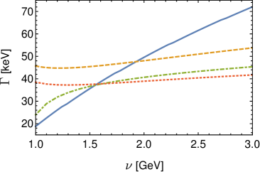
Figure 1: Leading order decay rate, $\Gamma_{E1}^{(0)}$, of the electric dipole transition $\chi_{b1}(1P)\to\gamma\Upsilon(1S)$. The renormalon cancellation is achieved order by order in the static potential which is exactly included when solving the Schrödinger equation. The panel (a) shows the case in which the renormalization group improved (RGI) version of the static potential is not used, whereas the panel (b) shows the results when the RGI potential is considered. The different curves in both panels represent the result coming from taking into account the Coulomb-like (solid blue), NLO (dashed orange), NNLO (dot-dashed green) and NNNLO (dotted red) terms in the static potential.

The panel (a) of Fig. 1 shows the leading order decay rate, $\Gamma_{E1}^{(0)}$, for the $\chi_{b1}(1P)\to\gamma\Upsilon(1S)$ transition computed when the static potential is included order by order in the Schrödinger equation. If one solves the Schrödinger equation numerically with only the Coulomb-like term of the static potential, one gets a leading order (LO) decay rate (solid blue curve) that depends strongly on the factorization scale (see Ref. [12] for details based on an analytical study). However, the $\nu$-scale dependence becomes mild as next-to-leading order (NLO) (dashed orange curve), NNLO (dot-dashed green curve) and NNNLO (dotted red curve) radiative corrections to the static potential are included in the Schrödinger equation.

The panel (b) of Fig. 1 shows the induced effect on the decay width once the correct log-arithmetically modulated short distance behavior (RGI) of the static potential is included properly. Now, the improvement in the convergence properties of the perturbative series is seen at $\nu\lesssim 1.7\,{\rm GeV}$. This is crucial in order to give final results for the decay rates since a low value of $\nu$, compatible with the typical momentum scale of the system under study, has to be chosen ($\nu=1.25\,\text{GeV}$). It is fair to mention that, in this final scheme, the dependence on the factorization scale for the NNNLO result seems to increase slightly.

The final decay width for the $\chi_{b1}(1P)\to\gamma\Upsilon(1S)$ process is shown in Fig. 2. The leading order non-relativistic decay rate is the dashed blue curve, the dot-dashed curve is taking into account the relativistic contributions stemming from higher order electromagnetic operators (Eq. (2) with $R^{S=1}(J)=0$) and the solid black one is including also the relativistic corrections to the wave function of the initial and final states (Eq. (2) with $R^{S=1}(J)\neq 0$).

One sees in Fig. 2 that the leading order decay width depends weakly on the factorization scale, it varies from $\Gamma\sim 33\,\text{ keV}$ at $\nu=1\,\text{GeV}$ to $\Gamma\sim 39\,\text{keV}$ at $\nu=3\,\text{GeV}$. This feature is translated to the case in which higher order electromagnetic operators are taken into account and also to the case in which wave function relativistic corrections are included. In fact, somewhat surprisingly, the $\nu$-dependence of our final result, $\sim 3\,\text{keV}$, is weaker than that of the leading order or even the one including higher order electromagnetic operators. A variation of $\sim 3\,\text{keV}$ over a total value of around $\sim 37\,\text{keV}$ represents a relative error of $\sim 8\%$ in our determination of the decay rate, being the biggest source of uncertainty.

It is clearly seen in Fig. 2 that both types of relativistic contributions are under control: they behave smoothly with respect the renormalization scale and produce corrections to the LO decay width which are relatively small. Another interesting feature of Fig. 2 is that the relativistic corrections induced by higher order electromagnetic operators tend to diminish the LO decay rate whereas the effect of the corrected initial and final wave functions is to increase it.

We have performed the same analysis than above to the electric dipole transitions $\chi_{b0}(1P)\to\gamma\Upsilon(1S)$, $\chi_{b2}(1P)\to\gamma\Upsilon(1S)$ and $h_{b}(1P)\to\gamma\Upsilon(1S)$. Similar conclusions than the ones already mentioned apply to these cases. Our final values for the electric dipole transitions $\chi_{bJ}(1P)\to\gamma\Upsilon(1S)$ with $J=0,1,2$ and $h_{b}(1P)\to\gamma\eta_{b}(1S)$ read

$$\Gamma(\chi_{b0}(1P)\to\gamma\Upsilon(1S)) =28^{+2}_{-1}~{}\text{keV}\,,$$ (8)

$$\Gamma(\chi_{b1}(1P)\to\gamma\Upsilon(1S)) =37^{+2}_{-1}~{}\text{keV}\,,$$ (9)

$$\Gamma(\chi_{b2}(1P)\to\gamma\Upsilon(1S)) =45^{+1}_{-1}~{}\text{keV}\,,$$ (10)

$$\Gamma(h_{b}(1P)\to\gamma\eta_{b}(1S)) =63^{+1}_{-1}~{}\text{keV}\,.$$ (11)

Because of the very mild dependence of our results on the renormalization scale $\nu$, the associated uncertainties are very small.

The Particle Data Group (PDG) [13] only reports the branching fractions of the E1 transitions studied herein. Since the total decay widths of the $\chi_{bJ}$ (with $J=0,1,2$) and $h_{b}(1P)$ mesons are not known, we cannot compare our theoretical results with experimental data. Nevertheless, we can use the branching fractions given by the PDG and our results for the decay rates of the electric dipole transitions to predict their total decay widths. The results are

$$\Gamma(\chi_{b0}(1P)) =1.6^{+0.3}_{-0.3}~{}\text{MeV}\,,\hskip 52.63777pt\Gamma(\chi_{b1}(1P))=110^{+9}_{-8}~{}\text{keV}\,,$$ (12)

$$\Gamma(\chi_{b2}(1P)) =234^{+15}_{-16}~{}\text{keV}\,,\hskip 56.9055pt\Gamma(h_{b}(1P))=121^{+14}_{-12}~{}\text{keV}\,.$$ (13)

These numbers could be of special interest for future experimental determinations. For instance, the Belle collaboration has recently reported an upper limit at 90% confidence level on the total decay width of the $\chi_{b0}(1P)$ [14]: $\Gamma(\chi_{b0}(1P))<2.4\,\text{MeV}$, which is well within the uncertainty band of our prediction.

4 Summary

We have performed the first numerical analysis of the electric dipole transitions $\chi_{bJ}(1P)\to\gamma\Upsilon(1S)$ with $J=0,1,2$ and $h_{b}(1P)\to\gamma\eta_{b}(1S)$ within the weak coupling version of a low-energy effective field theory called potential non-relativistic QCD.

This work has been supported by the DFG and the NSFC through funds provided to the Sino-German CRC 110 “Symmetries and the Emergence of Structure in QCD”, and by the DFG cluster of excellence “Origin and structure of the universe” (www.universe-cluster.de). J.S. acknowledges the financial support from the Alexander von Humboldt Foundation.

References

References

- [1] Segovia J, Steinbeiß er S and Vairo A in preparation: TUM-EFT 86/16
- [2] Segovia J, Ortega P G, Entem D R and Fernández F 2016 Phys. Rev. D93 074027
- [3] Pineda A and Soto J 1998 Nucl. Phys. Proc. Suppl. 64 428–432
- [4] Brambilla N, Pineda A, Soto J and Vairo A 2000 Nucl. Phys. B566 275
- [5] Brambilla N, Pineda A, Soto J and Vairo A 2005 Rev. Mod. Phys. 77 1423
- [6] Pineda A 2012 Prog. Part. Nucl. Phys. 67 735–785
- [7] Brambilla N, Pineda A, Soto J and Vairo A 2001 Phys. Rev. D63 014023
- [8] Pineda A and Segovia J 2013 Phys. Rev. D87 074024
- [9] Pietrulewicz P 2013 PoS ConfinementX, 135 (2012)
- [10] Martinez H E 2016 AIP Conf. Proc. 1701 050008
- [11] Brambilla N, Pietrulewicz P and Vairo A 2012 Phys. Rev. D85 094005
- [12] Steinbeiß er S and Segovia J 2017 EPJ Web Conf. 137 06026
- [13] Patrignani C et al. (Particle Data Group) 2016 Chin. Phys. C40 100001
- [14] Abdesselam A et al. (Belle) 2016 (Preprint 1606.01276)