We study physical consequences of adding orientifolds to the ABJ triality, which is among 3d ${\cal N}=6$ superconformal Chern-Simons theory known as ABJ theory, type IIA string in $AdS_{4}\times\mathbb{CP}^{3}$ and ${\cal N}=6$ supersymmetric (SUSY) Vasiliev higher spin theory in $AdS_{4}$. After adding the orientifolds, it is known that the gauge group of the ABJ theory becomes $O(N_{1})\times USp(2N_{2})$ while the background of the string theory is replaced by $AdS_{4}\times\mathbb{CP}^{3}/\mathbf{Z}_{2}$, and the supersymmetries in the both theories reduce to $\mathcal{N}=5$. We propose that adding the orientifolds to the ${\cal N}=6$ Vasiliev theory leads to $\mathcal{N}=5$ SUSY Vasiliev theory. It turns out that the $\mathcal{N}=5$ case is more involved because there are two formulations of the $\mathcal{N}=5$ Vasiliev theory with either $O$ or $USp$ internal symmetry. We show that the two $\mathcal{N}=5$ Vasiliev theories can be understood as certain projections of the $\mathcal{N}=6$ Vasiliev theory, which we identify with the orientifold projections in the Vasiliev theory. We conjecture that the $O(N_{1})\times USp(2N_{2})$ ABJ theory has the two vector model like limits: $N_{2}\gg N_{1}$ and $N_{1}\gg N_{2}$ which correspond to the semi-classical ${\cal N}=5$ Vasiliev theories with $O(N_{1})$ and $USp(2N_{2})$ internal symmetries respectively. These correspondences together with the standard AdS/CFT correspondence comprise the ABJ quadrality among the $\mathcal{N}=5$ ABJ theory, string/M-theory and two $\mathcal{N}=5$ Vasliev theories. We provide a precise holographic dictionary for the correspondences by comparing correlation functions of stress tensor and flavor currents. Our conjecture is supported by various evidence such as agreements of the spectra, one-loop free energies and SUSY enhancement on the both sides. We also predict the leading free energy of the ${\cal N}=5$ Vasiliev theory from the CFT side. As a byproduct, we give a derivation of the relation between the parity violating phase in the $\mathcal{N}=6$ Vasiliev theory and the parameters in the $\mathcal{N}=6$ ABJ theory, which was conjectured in [1].

WIS/01/17-AUG-DPPA

1 Introduction

At extremely high energy scale, string theory has been expected to exhibit a huge gauge symmetry as infinitely many massless higher spin (HS) particles emerge in the spectrum [2]. Then the usual string scale $1/\sqrt{\alpha^{\prime}}$ might arise as a dynamical scale via Higgsing the HS gauge symmetry. While these expectations are still speculative, there exist a self-consistent description of interacting HS gauge fields known as Vasiliev theory [3] independently of string theory. It is then natural to explore the relation between string theory and Vasiliev theory. The answer to this question remains largely open despite some attempts were made to directly connect Vasiliev theory to the tensionless limit of string (field) theory [4]. One of the indirect but steady steps towards answering this question is to reinterpret stringy objects or concepts in the framework of the Vasiliev theory. In this paper we aim at understanding orientifolds in the context of higher spin $AdS_{4}/{\rm CFT}_{3}$ correspondence between Vasiliev theory in $AdS_{4}$ and 3d conformal field theory (CFT) [5], which generalizes the usual AdS/CFT correspondence [6].

To be specific, we study physical consequences of adding orientifolds into the setup of ABJ triality [1, 7], which relates three apparently distinct theories as summarized in Fig. 1. It involves i) 3d $\mathcal{N}=6$ superconformal Chern-Simons (CS) theory called ${\cal N}=6$ ABJ theory [8, 9], which is the $U(N)_{k}\times U(N+M)_{-k}$ CS matter theory coupled to two bi-fundamental hyper multiplets; ii) Type IIA string theory in $AdS_{4}\times\mathbb{CP}^{3}$; iii) Parity-violating $\mathcal{N}=6$ supersymmetric (SUSY) Vasiliev theory with $U(N)$ internal symmetry in $AdS_{4}$. The $\mathcal{N}=6$ ABJ theory is expected to describe low energy dynamics of $N$ coincident M2-branes probing $\mathbf{C}^{4}/\mathbb{Z}_{k}$, together with $M$ coincident fractional M2-branes localized at the singularity. The M-theory background associated with this setup is $AdS_{4}\times S^{7}/\mathbf{Z}_{k}$ with the nontrivial 3-form holonomy $\int C_{3}\sim M/k$. For $k\ll N^{1/5}$, the M-theory circle shrinks and the M-theory is well approximated by type IIA string on $AdS_{4}\times\mathbb{CP}^{3}$. It is conjectured in [1, 7, 10] that the ${\cal N}=6$ ABJ theory is also dual to the ${\cal N}=6$ Vasiliev theory with $U(N)$ internal symmetry, in which the Newton constant $G_{N}\sim 1/M$. Especially the semi-classical approximation of the Vasiliev theory becomes accurate in the following limit of the ABJ theory

$$M,\,|k|\rightarrow\infty\quad{\rm with}\quad t\equiv\frac{M}{|k|}:{\rm finite}\quad{\rm and}\quad N:{\rm finite}~{}.$$ (1.1)

In this limit, the ABJ theory approaches a vector-like model which is the $U(N+M)$ SUSY CS theory coupled to $2N$ fundamental hyper multiplets with a weakly gauged $U(N)$ symmetry. This correspondence is a generalization of the duality between Vasiliev theory and $U(M)$ CS vector model [7, 11, 12, 13] to the case with weakly gauged flavor symmetries. In the ABJ triality, the fundamental string in the string theory is expected to be realized as “flux tube” solution or “glueball”-like bound state in the Vasiliev theory when the bulk coupling is large. The ${\cal N}=6$ ABJ triality was further investigated in [15, 16].

Now we add orientifolds into this scenario. For this purpose, it is convenient to begin with the type IIB brane construction of the $\mathcal{N}=6$ ABJ theory shown in Fig. 2 (see [8] for detail). There are four ways to consistently add orientifold 3-planes in this setup. Recall that there are four orientifold 3-planes $O3^{-}$, $O3^{+}$, $\widetilde{O3}^{-}$ and $\widetilde{O3}^{+}$, whose combinations with $N$ D3-branes lead to the gauge groups $O(2N)$, $USp(2N)$, $O(2N+1)$ and $USp(2N)$ respectively. Specifically, consistently adding $O3^{\pm}$ into the ${\cal N}=6$ set up with $k\rightarrow 2k$ leads to the $\mathcal{N}=5$ ABJ theory with the gauge group $O(N_{1})_{2k}\times USp(2N_{2})_{-k}$, where $N_{1}$ is an even integer. The odd $N_{1}$ case is obtained by adding $\widetilde{O3}^{\pm}$. In summary, the ${\cal N}=5$ ABJ theory can have the four types of the gauge group:

1. $O(2N)_{2k}\times USp(2N+2M)_{-k}$ ,

2. $O(2N+2M)_{2k}\times USp(2N)_{-k}$ ,

3. $O(2N+1)_{2k}\times USp(2N+2M)_{-k}$ ,

4. $O(2N+2M+1)_{2k}\times USp(2N)_{-k}$ .

The M-theory background dual to the ${\cal N}=5$ ABJ theory is given by $AdS_{4}\times S^{7}/\hat{\mathbf{D}}_{k}$. Similar to the $\mathcal{N}=6$ case, the M-theory circle shrinks for $k\ll N^{1/5}$ and the M-theory is well approximated by the type IIA string in $AdS_{4}\times\mathbb{CP}^{3}/\mathbf{Z}_{2}$ with the NS-NS 2-form holonomy $\int B_{2}\propto M/k$. While this is well known, inspired by the $\mathcal{N}=6$ ABJ triality it is natural to ask whether the $\mathcal{N}=5$ ABJ theory also admits some dual higher spin description. To the best of our knowledge, this aspect has not been studied in literature. The focus of this paper is to establish the AdS/CFT correspondence among the $\mathcal{N}=5$ ABJ theory, type IIA string in $AdS_{4}\times\mathbb{CP}^{3}/\mathbf{Z}_{2}$ and $\mathcal{N}=5$ Vasiliev theory in $AdS_{4}$ with internal symmetry.

Figure 1: Summary of the $\mathcal{N}=6$ ABJ triality.

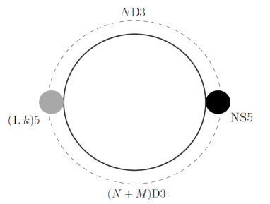
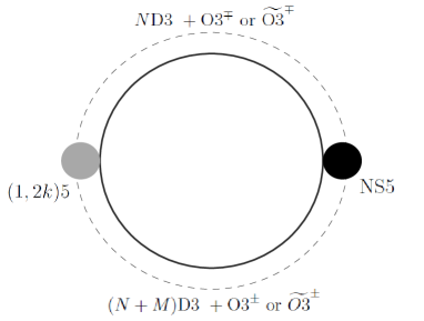
Figure 2: The type IIB brane constructions for the ABJ theories. All the objects share three common dimensions and the D3-branes wind the $S^{1}$-direction. [Left] The $\mathcal{N}=6$ case with the gauge group $U(N)_{k}\times U(N+M)_{-k}$. [Right] The $\mathcal{N}=5$ case with the gauge group $O(N_{1})_{2k}\times USp(2N_{2})_{-k}$ where $({\rm rank}[O(N_{1})],N_{2})$ $=$ $(N,N+M)$ or $(N+M,N)$.

We carry out this by first constructing the ${\cal N}=5$ Vasiliev theory. As shown in sec. 2, there are two types of allowed internal symmetry for the ${\cal N}=5$ HS theory, which is either $O$ or $USp$ group. These two possibilities should correspond to two vector limits of the ${\cal N}=5$ ABJ theory. Recalling that the gauge group of the ${\cal N}=5$ ABJ theory is $O(N_{1})\times USp(N_{2})$, we first propose that the $\mathcal{N}=5$ ABJ theory is dual to the semi-classical $\mathcal{N}=5$ Vasiliev theory with $O(N_{1})$ internal symmetry in the following limit

$$N_{2}=|O(N_{1})|+M\,,\quad M,\,|k|\rightarrow\infty\quad{\rm with}\quad t\equiv\frac{M}{|k|}\quad{\rm and}\quad N_{1}:{\rm finite}~{},$$ (1.2)

where $|O(N_{1})|$ is the rank of $O(N_{1})$. We also propose that the second limit corresponding to the semi-classical Vasiliev theory with $USp(2N_{2})$ internal symmetry is

$$|O(N_{1})|=N_{2}+M\,,\quad M,\,|k|\rightarrow\infty\quad{\rm with}\quad t\equiv\frac{M}{|k|}\quad{\rm and}\quad N_{2}:{\rm finite}~{}.$$ (1.3)

The correspondence between the HS and CFT parameters is as follows. As the $\mathcal{N}=5$ ABJ theory has the three parameters $(k,M,N)$, the $\mathcal{N}=5$ Vasiliev theory also has the three parameters $(G_{N},\theta,N)$, where $G_{N}$ is the Newton constant, $\theta$ is the parity-violating phase and $N$ is the rank of the internal symmetry group. We derive the precise holographic dictionary by matching correlation functions of stress tensor and flavor symmetry currents, which we compute on the CFT side by SUSY localization [18]. As we will discuss in sec. 4.7, the analysis of the stress tensor correlation function suggests that the Newton constant $G_{N}$ is related to $M$ by

$$\frac{G_{N}}{L_{\rm AdS}^{2}}=\frac{t}{M\sin\pi t},$$ (1.4)

while the comparison of the flavor current correlation function indicates that the parity-violating phase $\theta$ is related to $t$ by

$$\theta=\frac{\pi t}{2}.$$ (1.5)

We also show that the relation (1.5) is true also for the $\mathcal{N}=6$ ABJ triality, where (1.5) was conjectured but not proven in [1]. In the limit (1.2), the $\mathcal{N}=5$ ABJ theory approaches the $USp(2N_{2})$ SUSY CS theory coupled to $N_{1}$ fundamental hyper multiplets with a weakly gauged $O(N_{1})$ symmetry while the limit (1.3) provides the $O(N_{1})$ SUSY CS theory coupled to $N_{2}$ fundamental hyper multiplets with a weakly gauged $USp(2N_{2})$ symmetry. Our correspondence is a generalization of the duality between Vasiliev theory and $O(M)$ or $USp(2M)$ CS vector model [11, 19] to the case with weakly gauged flavor symmetries. As in the $\mathcal{N}=6$ case, we expect that the fundamental string in the dual string theory is realized as a “flux tube” in the $\mathcal{N}=5$ Vasiliev theory. Combined with the standard AdS/CFT correspondence, we conjecture the duality-like relations among the four apparently different theories, namely the $\mathcal{N}=5$ ABJ theory, string/M-theory and two $\mathcal{N}=5$ Vasiliev theories with $O$ and $USp$ internal symmetries. Thus we shall call it ABJ quadrality as summarized in Fig. 3. Since the $\mathcal{N}=5$ Vasiliev theories with $O$ and $USp$ internal symmetries have the bulk ’t Hooft couplings $\sim N_{1}/N_{2}$ and $\sim N_{2}/N_{1}$ respectively, the relation between the two Vasiliev theories looks like a strong-weak duality of the bulk ’t Hooft coupling as a result.

Figure 3: Summary of our proposal on the ABJ quadrality among the $\mathcal{N}=5$ ABJ theory, string/M-theory and two $\mathcal{N}=5$ Vasiliev theories. The parameter $N$ is the rank of “smaller” gauge group, namely $N={\rm min}({\rm rank}(O(N_{1})),N_{2})$. The main difference from the $\mathcal{N}=6$ case is that we have two higher spin limits corresponding to the $\mathcal{N}=5$ Vasiliev theories with different internal symmetries.

We have various evidence for the proposed correspondence between the $\mathcal{N}=5$ ABJ theory and Vasiliev theory. First we will see in sec. 4.3 that the spectrum of higher spin particles in the ${\cal N}=5$ Vasiliev theory agrees with that of the higher spin currents in the ${\cal N}=5$ ABJ theory.

Second, there is a non-trivial consistency among the spectra, $\mathcal{N}=6$ ABJ triality and “orientifold projection”. It is known [9] that the ${\cal N}=5$ ABJ theory can be understood as a certain projection of the ${\cal N}=6$ ABJ theory. We show in sec. 3 that one can also derive the ${\cal N}=5$ Vasiliev theory by applying a projection on the ${\cal N}=6$ Vasiliev theory, which we identify with the counterpart of the orientifold projection in the Vasiliev theory. Roughly speaking, the projection acts on both the $R$-symmetry part and the internal symmetry part of master fields and preserves the $USp(4)\subset SU(4)$ $R$-symmetry. More precisely, this is achieved by projection conditions (3.5) induced by two automorphisms of the ${\cal N}=6$ HS algebra. Then we prove in sec. 4.4 that the action of the projection on the higher spin currents in the ABJ theory is the same as the one on the Vasiliev theory. For example, the ${\cal N}=5$ Vasiliev theory contains two short multiplets: a usual supergravity (SUGRA) multiplet and gravitino multiplet. The gravitino multiplet carries adjoint representation of $O$ or $USp$ internal symmetry. These two short ${\cal N}=5$ supermultiplets appear once imposing the projection conditions on the $U(N)$ adjoint ${\cal N}=6$ SUGRA multiplet in the $\mathcal{N}=6$ Vasiliev theory.

Third, SUSY enhancement occurs on the both sides under the same circumstance as discussed in sec. 4.5. It is known [22, 23] that the SUSY of the $O(N_{1})_{2k}\times USp(2N_{2})_{-k}$ ABJ theory is enhanced from $\mathcal{N}=5$ to $\mathcal{N}=6$ when $N_{1}=2$. Interestingly the dual $\mathcal{N}=5$ Vasiliev theory with the $O(N_{1})$ internal symmetry has also enhanced $\mathcal{N}=6$ SUSY in the $O(2)$ case as explained in sec. 2.1.

Finally we find agreement of the sphere free energies on the both sides at $\mathcal{O}(\log{G_{N}})$ up to a subtlety in the comparison. The subtlety is that the free energy of the ABJ theory behaves as $\mathcal{O}(M^{2})$ while the one of the Vasiliev theory should behave as $\mathcal{O}(G_{N}^{-1})=\mathcal{O}(M)$. Therefore the ABJ theory has apparently more degrees of freedom than the Vasiliev theory and we have to subtract some degrees of freedom appropriately. This problem appears also in CS matter theory coupled to fundamental matters [7, 13]. and the $\mathcal{N}=6$ ABJ theory [15]. We propose that the free energy which should be compared to the one in Vasiliev theory is

$$F^{\rm vec}_{N,M}\equiv-\log\frac{|Z_{{\rm G}_{N,M}}|}{|Z_{{\rm G}_{0,M}}|}~{},$$ (1.6)

where ${\rm G}_{N,M}$ denotes the gauge group of each case in (4.10) and $Z_{{\rm G}_{N,M}}$ is the sphere partition function of the ABJ theory with the gauge group ${\rm G}_{N,M}$. This quantity satisfies the following reasonable properties: i) $1/M$-expansion starts at $\mathcal{O}(M)$; ii) Invariance under Seiberg-like duality; iii) The $\mathcal{O}(\log{M})$ term agrees with that in the one-loop free energy of the $\mathcal{N}=5$ Vasiliev theory. Our proposal implies that the open string degrees of freedom corresponding to the Vasiliev theory are given by Fig. 4 from the viewpoint of the brane construction. Utilizing localization method and matrix model technique, we compute $F^{\rm vec}_{N,M}$ up to the ${\cal O}(1)$ term in $1/M$ expansion but exact in $t$. Using this result and our holographic dictionary, we propose that the free energy of the ${\cal N}=5$ Vasiliev theory with $O(N_{1})$ or $USp(2N_{2})$ internal symmetry takes the form in the small $G_{N}$ expansion

$$F_{\rm HS}=\frac{8L^{2}_{\rm AdS}I(\theta)}{G_{N}\pi\sin 2\theta}-\frac{{\rm min}\{{\rm dim}O(N_{1}),{\rm dim}USp(2N_{2})\}}{2}\log{G_{N}}+\mathcal{O}(1)~{},$$ (1.7)

where

$$I(x)={\rm Im}\Bigl{[}{\rm Li}_{2}({\rm i}\tan{x})\Bigr{]}-x\log{\tan{x}}~{}.$$ (1.8)

The first term in (1.7) should correspond to the tree level action of Vasiliev theory evaluated on $AdS_{4}$ which we cannot currently compare with any results in literature, since the full action of the Vasiliev theory has not been constructed. Hence we regard our result as prediction to the on-shell action of the $\mathcal{N}=5$ Vasiliev theory in $AdS_{4}$. As mentioned above, the second term agrees with the one-loop free energy of the Vasiliev theory on $AdS_{4}$, which is free of logarithmic divergences [24] and equal to $(-1/2)$ times the number of bulk spin-1 gauge fields obeying the mixed boundary condition [25].

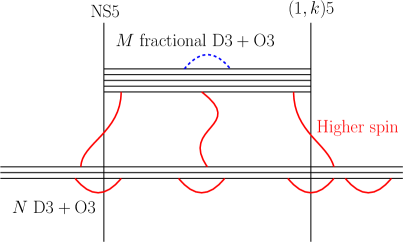
Figure 4: Identification of degrees of freedom corresponding to those of the Vasiliev theory from the viewpoint of the brane construction. Strings denoted by the red solid lines are the HS degrees of freedom while the blue dashed line is what we are subtracting.

In Section 6, we summarize and discuss possible extensions of this work.

2 $\mathcal{N}=5$ supersymmetric Vasiliev theory

In this section, we explain some details on the $\mathcal{N}=5$ SUSY Vasiliev theory. First we construct the $\mathcal{N}=5$ Vasiliev theory for the two cases with $O(N)$ and $USp(2N)$ internal symmetries. Next we linearize the $\mathcal{N}=5$ Vasiliev theory around the $AdS_{4}$ vacuum preserving $\mathcal{N}=5$ SUSY. We explicitly write down the equations of motion, gauge transformations and SUSY transformations around the $AdS_{4}$ vacuum.

2.1 Construction

Here we construct the $\mathcal{N}=5$ Vasiliev theory. The ${\cal N}=5$ Vasiliev theory is based on $husp(4;4|4)$ SUSY higher spin algebra [26], which contains the maximal compact subalgebra $usp(4)\oplus usp(4)$. As we will explain, this theory admits either $O(N)$ or $USp(2N)$ as an internal symmetry. We begin with aspects which are common between the two cases and then specify the internal symmetries. Four dimensional Vasiliev theory is realized by introducing the spinorial oscillators $(Y,Z)=(y,\bar{y},z,\bar{z})$ with the associative but non-commutative $\star$-product defined as

$$\star\equiv\exp[{\rm i}C^{\alpha\beta}(\overset{\leftarrow}{\partial}_{y^{\alpha}}+\overset{\leftarrow}{\partial}_{z^{\alpha}})(\overset{\rightarrow}{\partial}_{y^{\beta}}-\overset{\rightarrow}{\partial}_{z^{\beta}})+{\rm i}C^{\dot{\alpha}\dot{\beta}}(\overset{\leftarrow}{\partial}_{\bar{y}^{\dot{\alpha}}}+\overset{\leftarrow}{\partial}_{\bar{z}^{\dot{\alpha}}})(\overset{\rightarrow}{\partial}_{\bar{y}^{\dot{\beta}}}-\overset{\rightarrow}{\partial}_{\bar{z}^{\dot{\beta}}})]~{},$$ (2.1)

where $C^{\alpha\beta}=-i\epsilon^{\alpha\beta}$ and $C^{\dot{\alpha}\dot{\beta}}=-i\epsilon^{\dot{\alpha}\dot{\beta}}$. The indices $\alpha,\beta=1,2$ and $\dot{\alpha},\dot{\beta}=1,2$ serve as indices of two-component spinors. According to this definition, we have the following identities

$$\begin{split}y^{\alpha}\star y^{\beta}=y^{\alpha}y^{\beta}+{\rm i}C^{\alpha\beta}~{}&,~{}~{}z^{\alpha}\star z^{\beta}=z^{\alpha}z^{\beta}-{\rm i}C^{\alpha\beta}~{},\\ [y^{\alpha},f]_{\star}=2{\rm i}C^{\alpha\beta}\partial_{y^{\beta}}f~{}&,~{}~{}[z^{\alpha},f]_{\star}=-2{\rm i}C^{\alpha\beta}\partial_{z^{\beta}}f~{},\\ \{y^{\alpha},f\}_{\star}=2y^{\alpha}f-2{\rm i}C^{\alpha\beta}\partial_{z^{\beta}}f~{}&,~{}~{}\{z^{\alpha},f\}_{\star}=2z^{\alpha}f+2{\rm i}C^{\alpha\beta}\partial_{y^{\beta}}f~{},\end{split}$$ (2.2)

where $f$ is arbitrary function of $(x,Y,Z)$.

In the $\mathcal{N}=5$ Vasiliev theory, we take fields to be $8N\times 8N$ matrices, which are tensor products of $8\times 8$ and $N\times N$ parts. Roughly speaking, the $8\times 8$ part is needed to introduce fermions and the size of this part depends on the type of SUSY while the $N\times N$ part $\mathcal{M}$ describes internal symmetry and properties of $\mathcal{M}$ depend on the internal symmetry under consideration. We describe the $8\times 8$ part in terms of the six Grassmannian variables $(\xi^{1},...,\xi^{5},\eta)$ which commute with $(Y,Z)$ and satisfy the Clifford algebra

$$\{\xi^{i},\xi^{j}\}=\delta^{ij}~{},~{}~{}(\eta)^{2}=1~{},~{}~{}\{\eta,\xi^{i}\}=0~{}.$$ (2.3)

Viewing $(\xi^{i},\eta)$ as the $SO(6)$ gamma matrices, we can realize the $8\times 8$ part as a sum of products of $(\xi^{i},\eta)$.

The Vasiliev system is described by so-called master fields, which consist of the connection 1-form $A$ in $(x,Z)$ space and the 0-form $\Phi$ given by

$$A=A(x,y,\bar{y},z,\bar{z},\xi^{i},\eta)=\Omega_{\mu}dx^{\mu}+S_{\alpha}dz^{\alpha}+S_{\dot{\alpha}}d\bar{z}^{\dot{\alpha}}~{},\quad\Phi=\Phi(x,y,\bar{y},z,\bar{z},\xi^{i},\eta)~{}.$$ (2.4)

They obey the spin-statistics condition

$$\pi\bar{\pi}\pi_{\xi}\pi_{\eta}(A,\Phi)=(A,\Phi)~{},$$ (2.5)

where $\pi$’s are the homomorphisms of the $\star$-product defined by

$$\pi(y,\bar{y},z,\bar{z})=(-y,\bar{y},-z,\bar{z}),\quad\bar{\pi}(y,\bar{y},z,\bar{z})=(y,-\bar{y},z,-\bar{z}),\quad\pi_{\xi}(\xi^{i})=-\xi^{i},~{}\pi_{\eta}(\eta)=-\eta.$$ (2.6)

The master fields contain both dynamical and auxiliary degrees of freedom. The physical degrees of freedom are contained in the $Z$ independent part of $\Omega_{\mu}$ and $\Phi$ while $S_{\alpha}$ and $S_{\dot{\alpha}}$ have only auxiliary degrees of freedom. When the fields carry non-trivial representations of the internal symmetry, the $Z$ independent parts of $\Omega_{\mu}$ and $\Phi$ have the general expansions

$$\begin{split}&\Omega_{\mu}|_{Z=0}=\sum_{\begin{subarray}{c}p,q\geq 0\\ k=0,...,5\end{subarray}}\frac{1}{k!}\Big{(}\Omega_{\mu,i_{1}\cdots i_{k}}(p,q)\xi^{i_{1}\cdots i_{k}}+\Omega^{\prime}_{\mu,i_{1}\cdots i_{k}}(p,q)\xi^{i_{1}\cdots i_{k}}\eta\Big{)}\otimes\mathcal{M}~{},\\ &\Phi|_{Z=0}=\sum_{\begin{subarray}{c}p,q\geq 0\\ k=0,...,5\end{subarray}}\frac{1}{k!}\Big{(}\Phi_{i_{1}\cdots i_{k}}(p,q)\xi^{i_{1}\cdots i_{k}}+\Phi^{\prime}_{i_{1}\cdots i_{k}}(p,q)\xi^{i_{1}\cdots i_{k}}\eta\Big{)}\otimes\mathcal{M}~{},\end{split}$$ (2.7)

where $\xi^{i_{1}\cdots i_{k}}=\xi^{i_{1}}\cdots\xi^{i_{k}}$ and

$${\cal P}(p,q)=\frac{1}{p!q!}{\cal P}_{\alpha_{1}\cdots\alpha_{p}\dot{\alpha}_{1}\cdots\dot{\alpha}_{q}}y^{\alpha_{1}}\cdots y^{\alpha_{p}}\bar{y}^{\dot{\alpha}_{1}}\cdots\bar{y}^{\dot{\alpha}_{q}}~{}.$$ (2.8)

The spin $s$ gauge fields are described by the $p+q=2s-2$ components of $\Omega_{\mu}|_{Z=0}$, in which the $p=q$ and $|p-q|=1$ components give rise to the (generalized) vierbein and gravitini respectively, while the $|p-q|>1$ components correspond to the spin connections. The matter fields with spin $s\leq\frac{1}{2}$ arise as components of $\Phi|_{Z=0}$ with $p+q\leq 1$. The remaining components in $\Phi|_{Z=0}$ are auxiliary and related to the Weyl tensors of the physical fields and their derivatives via equations of motion.

2.1.1 $O(N)$ internal symmetry

Let us specify our internal symmetry to $O(N)$. First we take $\mathcal{M}$ to be the $N\times N$ real matrix associated with the internal symmetry $O(N)$, which can be decomposed into symmetric and antisymmetric parts. Next we define the $\tau$ map as

$$\begin{split}\tau(y,\bar{y},z,\bar{z})=({\rm i}y,{\rm i}\bar{y},-{\rm i}z,-{\rm i}\bar{z})~{},\quad\tau(\xi^{i})={\rm i}\xi^{i}~{},\quad\tau(\eta)=-{\rm i}\eta~{},~{}~{}\end{split}$$ (2.9)

and

$$\tau(\mathcal{M})=\mathcal{M}^{T}~{}.$$ (2.10)

The conditions (2.9) will be imposed also for the case with $USp(2N)$ internal symmetry while the condition for $\mathcal{M}$ will differ from (2.10). Then we require the master fields to satisfy the reality condition

$$A^{\dagger}=-A\,,\quad\Phi^{\dagger}=\pi(\Phi)\Gamma~{},$$ (2.11)

and the $\tau$-condition

$$\tau(A)=-A\,,\quad\tau(\Phi)=\bar{\pi}(\Phi)~{},$$ (2.12)

where $\Gamma={\rm i}\xi^{1}\cdots\xi^{5}\eta$ and $\Gamma^{2}=1$. The ${\dagger}$ acts on ($Y,Z,\xi^{i},\eta$) and $\mathcal{M}$ according to

$$y^{\alpha{\dagger}}=\bar{y}^{\dot{\alpha}}~{},~{}~{}z^{\alpha{\dagger}}=-\bar{z}^{\dot{\alpha}}~{},~{}~{}\xi^{i{\dagger}}=\xi^{i}~{},~{}~{}\eta^{\dagger}=\eta~{},~{}~{}(\xi^{i}\xi^{j})^{\dagger}=\xi^{j}\xi^{i}~{},~{}~{}(\xi^{i}\eta)^{\dagger}=\eta\xi^{i}~{},~{}~{}\mathcal{M}^{\dagger}=(\mathcal{M}^{T})^{\ast}.$$ (2.13)

The $\tau$- and reality conditions affect the spectrum of physical degrees of freedom. We now analyze their consequences on $\Omega_{\mu}|_{Z=0}$. First let us consider symmetric part of $\mathcal{M}$, which corresponds to two index symmetric representation of $O(N)$. Noting that acting $\tau$ on $\Omega_{\mu,i_{1}\cdots,i_{k}}\xi^{i_{1}\cdots i_{k}}$ gives the extra factor $i^{p+q+k}$, as a consequence, the $\tau$-condition requires

$$\begin{split}&\Omega_{\mu}|_{Z=0}=\sum^{\infty}_{n=0}\Big{\{}\sum_{p+q=4n}\Big{(}{\textstyle\frac{1}{2!}}\Omega_{\mu,ij}(p,q)\xi^{ij}+{\textstyle\frac{1}{3!}}\Omega^{\prime}_{\mu,ijk}(p,q)\xi^{ijk}\eta\Big{)}\\ &\quad+\sum_{p+q=4n+1}\Big{(}\Omega_{\mu,i}(p,q)\xi^{i}+{\textstyle\frac{1}{5!}}\Omega_{\mu,i_{1}\cdots i_{5}}(p,q)\xi^{i_{1}\cdots i_{5}}+{\textstyle\frac{1}{2!}}\Omega^{\prime}_{\mu,ij}(p,q)\xi^{ij}\eta\Big{)}\\ &\quad+\sum_{p+q=4n+2}\Big{(}\Omega_{\mu}(p,q)+{\textstyle\frac{1}{4!}}\Omega_{\mu,i_{1}\cdots i_{4}}(p,q)\xi^{i_{1}\cdots i_{4}}+\Omega^{\prime}_{\mu,i}(p,q)\xi^{i}\eta+{\textstyle\frac{1}{5!}}\Omega^{\prime}_{\mu,i_{1}\cdots i_{5}}(p,q)\xi^{i_{1}\cdots i_{5}}\eta\Big{)}\\ &\quad+\sum_{p+q=4n+3}\Big{(}{\textstyle\frac{1}{3!}}\Omega_{\mu,ijk}(p,q)\xi^{ijk}+\Omega^{\prime}_{\mu}(p,q)\eta+{\textstyle\frac{1}{4!}}\Omega^{\prime}_{\mu,i_{1}\cdots i_{4}}(p,q)\xi^{i_{1}\cdots i_{4}}\eta\Big{)}\Big{\}}\,.\end{split}$$ (2.14)

The reality condition further requires

$${\Omega}^{\dagger}_{\mu,i_{1}\cdots i_{k}}(p,q)=(-1)^{\frac{k(k-1)}{2}+1}\Omega_{\mu,i_{1}\cdots i_{k}}(q,p)~{},\quad{\Omega^{\prime}}^{\dagger}_{\mu,i_{1}\cdots i_{k}}(p,q)=(-1)^{\frac{k(k+1)}{2}+1}\Omega^{\prime}_{\mu,i_{1}\cdots i_{k}}(q,p)~{}.$$ (2.15)

The analysis for $\Phi$ is similar and the result for $p\geq q$ is

$$\Phi|_{Z=0}=\left\{\begin{matrix}&~{}\Phi(p,q)+{\textstyle\frac{1}{4!}}\Phi_{i_{1}\cdots i_{4}}(p,q)\xi^{i_{1}\cdots i_{4}}+\Phi^{\prime}_{i}(p,q)\xi^{i}\eta+{\textstyle\frac{1}{5!}}\Phi^{\prime}_{i_{1}\cdots i_{5}}(p,q)\xi^{i_{1}\cdots i_{5}}\eta&{p-q=0\ \mbox{mod}\ 4}\\ &~{}{\textstyle\frac{1}{3!}}\Phi_{ijk}(p,q)\xi^{ijk}+\Phi^{\prime}(p,q)\eta+{\textstyle\frac{1}{4!}}\Phi^{\prime}_{i_{1}\cdots i_{4}}(p,q)\xi^{i_{1}\cdots i_{4}}\eta&{p-q=1\ \mbox{mod}\ 4}\\ &~{}{\textstyle\frac{1}{2!}}\Phi_{ij}(p,q)\xi^{ij}+{\textstyle\frac{1}{3!}}\Phi^{\prime}_{ijk}(p,q)\xi^{ijk}\eta&{p-q=2\ \mbox{mod}\ 4}\\ &~{}\Phi_{i}(p,q)\xi^{i}+{\textstyle\frac{1}{5!}}\Phi_{i_{1}\cdots i_{5}}(p,q)\xi^{i_{1}\cdots i_{5}}+{\textstyle\frac{1}{2!}}\Phi^{\prime}_{ij}(p,q)\xi^{ij}\eta&{p-q=3\ \mbox{mod}\ 4}\end{matrix}\right.$$ (2.16)

where due to the reality condition,

$${\Phi}^{\dagger}(p,p)={\textstyle\frac{{\rm i}}{5!}}(-1)^{p+1}\varepsilon^{ijklm}\Phi^{\prime}_{ijklm}(p,p)~{},\quad{\Phi}^{\dagger}_{ijkl}(p,p)={\rm i}(-1)^{p+1}\,\varepsilon_{ijklm}\Phi^{\prime m}(p,p)~{}.$$ (2.17)

The $p<q$ components of $\Phi|_{Z=0}$ are related to the $p>q$ ones via the reality condition (2.12). The $SO(5)$ indices are raised and lowered by $\delta^{ij}$. We summarize the final result in table 1. Note that in SUSY Vasiliev theory with internal symmetry, fields in the usual SUGRA multiplet are extended to matrices, and only the singlet components under the internal symmetry, namely the trace part, are related to the operators inside the dual CFT stress tensor multiplet via holography. The Konishi multiplet and other higher spin multiplets exhibit the standard long multiplet pattern with the spin range being ${\textstyle\frac{5}{2}}$.

${}_{\ell}\backslash s$	$0$	$\frac{1}{2}$	$1$	$\frac{3}{2}$	$2$	$\frac{5}{2}$	$3$	$\frac{7}{2}$	$4$	$\frac{9}{2}$	$5$	$\frac{11}{2}$	$6$	$\cdots$
$0$	$\underline{5}+\underline{5}$	$\underline{1}+\underline{10}$	$\underline{10}+10$	$\underline{5}+10$	$\underline{1}+5$	$1$
$1$	$1+1$	$5$		$1$	$5+1$	$10+5$	$10+10$	$5+10$	$1+5$	$1$
$2$								$1$	$5+1$	$10+5$	$10+10$	$5+10$	$1+5$	$\cdots$
$3$												$1$	$5+1$	$\cdots$
$\vdots$

Table 1: The spectrum of physical fields carrying symmetric $\cal{M}$ in the $\mathcal{N}=5$ Vasiliev theory with the $O(N)$ internal symmetry in the language of $SO(5)$ representations. For $s\geq 1$ fields, the level $\ell$ is related to $s$ by $s=2\ell+2-k/2+r/2$ where $k$ is the number of $\xi$s and $r$ is the number of $\eta$. The values of $\ell$ are assigned to spin-0, 1/2 fields such that fields belonging to the same supermultiplet are labeled by the same $\ell$. The underlines denote the fields in the $\mathcal{N}=5$ SUGRA multiplet. This table also provides the spectrum of physical fields associated with antisymmetric ${\cal J}\cal{M}$ in the case with $USp(2N)$ internal symmetry.

Next we consider anti-symmetric part of $\mathcal{M}$ corresponding to two index anti-symmetric representation of $O(N)$. Then imposing $\tau$-condition leads to

$$\begin{split}&\Omega_{\mu}|_{Z=0}=\sum^{\infty}_{n=0}\Big{\{}\sum_{p+q=4n+1}\Big{(}{\textstyle\frac{1}{3!}}\Omega_{\mu,ijk}(p,q)\xi^{ijk}+\Omega^{\prime}_{\mu}(p,q)\eta+{\textstyle\frac{1}{4!}}\Omega^{\prime}_{\mu,i_{1}\cdots i_{4}}(p,q)\xi^{i_{1}\cdots i_{4}}\eta\Big{)}\\ &\quad+\sum_{p+q=4n+2}\Big{(}{\textstyle\frac{1}{2!}}\Omega_{\mu,ij}(p,q)\xi^{ij}+{\textstyle\frac{1}{3!}}\Omega^{\prime}_{\mu,ijk}(m,n)\xi^{ijk}\eta\Big{)}\\ &\quad+\sum_{p+q=4n+3}\Big{(}\Omega_{\mu,i}(p,q)\xi^{i}+{\textstyle\frac{1}{5!}}\Omega_{\mu,i_{1}\cdots i_{5}}(p,q)\xi^{i_{1}\cdots i_{5}}+{\textstyle\frac{1}{2!}}\Omega^{\prime}_{\mu,ij}(p,q)\xi^{ij}\eta\Big{)}\\ &\quad+\sum_{p+q=4n}\Big{(}\Omega_{\mu}(p,q)+{\textstyle\frac{1}{4!}}\Omega_{\mu,i_{1}\cdots i_{4}}(p,q)\xi^{i_{1}\cdots i_{4}}+\Omega^{\prime}_{\mu,i}(p,q)\xi^{i}\eta+{\textstyle\frac{1}{5!}}\Omega^{\prime}_{\mu,i_{1}\cdots i_{5}}(p,q)\xi^{i_{1}\cdots i_{5}}\eta\Big{)}\Big{\}}\,,\end{split}$$ (2.18)

and the reality conditions requires

$${\Omega}^{\dagger}_{\mu,i_{1}\cdots i_{k}}(p,q)=(-1)^{\frac{k(k-1)}{2}}\Omega_{\mu,i_{1}\cdots i_{k}}(q,p)~{},\quad{\Omega}^{\prime\dagger}_{\mu,i_{1}\cdots i_{k}}(p,q)=(-1)^{\frac{k(k+1)}{2}}\Omega^{\prime}_{\mu,i_{1}\cdots i_{k}}(q,p)~{}.$$ (2.19)

Similarly, $\Phi|_{Z=0}$ for $p\geq q$ possesses the expansion

$$\Phi|_{Z=0}=\left\{\begin{matrix}&~{}{\textstyle\frac{1}{2!}}\Phi_{ij}(p,q)\xi^{ij}+{\textstyle\frac{1}{3!}}\Phi^{\prime}_{ijk}(p,q)\xi^{ijk}\eta&{p-q=0\ \mbox{mod}\ 4}\\ &~{}\Phi_{i}(p,q)\xi^{i}+{\textstyle\frac{1}{5!}}\Phi_{i_{1}\cdots i_{5}}(p,q)\xi^{i_{1}\cdots i_{5}}+{\textstyle\frac{1}{2!}}\Phi^{\prime}_{ij}(p,q)\xi^{ij}\eta&{p-q=1\ \mbox{mod}\ 4}\\ &~{}\Phi(p,q)+{\textstyle\frac{1}{4!}}\Phi_{i_{1}\cdots i_{4}}(p,q)\xi^{i_{1}\cdot i_{4}}+\Phi^{\prime}_{i}(p,q)\xi^{i}\eta+{\textstyle\frac{1}{5!}}\Phi^{\prime}_{i_{1}\cdots i_{5}}(p,q)\xi^{i_{1}\cdots i_{5}}\eta&{p-q=2\ \mbox{mod}\ 4}\\ &~{}{\textstyle\frac{1}{3!}}\Phi_{ijk}(p,q)\xi^{ijk}+\Phi^{\prime}(p,q)\eta+{\textstyle\frac{1}{4!}}\Phi^{\prime}_{i_{1}\cdots i_{4}}(p,q)\xi^{i_{1}\cdots i_{4}}\eta&{p-q=3\ \mbox{mod}\ 4}\end{matrix}\right.$$ (2.20)

where the reality condition constrains

$${\Phi}^{\dagger}_{ij}(p,p)={\textstyle\frac{{\rm i}}{3!}}(-1)^{p}\,\varepsilon_{ijklm}\Phi^{\prime klm}(p,p)~{}.$$ (2.21)

The $p<q$ components of $\Phi|_{Z=0}$ are related to the $p>q$ ones through the reality condition (2.12). The final result is summarized in Table 2. Especially we have the gravitino multiplet, which is underlined in Table 2. The gravitino multiplet for $N=2$ is special because the two-index anti-symmetric representation of $O(N)$ is singlet. Together with the $O(2)$-singlet $\mathcal{N}=5$ SUGRA multiplet, it comprises the $\mathcal{N}=6$ SUGRA multiplet singlet under the internal symmetry. This indicates that the supersymmetry of the $O(2)$ case is enhanced from $\mathcal{N}=5$ to $\mathcal{N}=6$. For $N\neq 2$, the existence of the gravitino multiplet does not imply the SUSY enhancement since SUSY generators should be singlet under the internal symmetry and the gravitino multiplet does not contain any singlet parts. We will come back to this point in sec. 4.5.

${}_{\ell}\backslash s$	$0$	$\frac{1}{2}$	$1$	$\frac{3}{2}$	$2$	$\frac{5}{2}$	$3$	$\frac{7}{2}$	$4$	$\frac{9}{2}$	$5$	$\frac{11}{2}$	$6$	$\cdots$
$0$	$\underline{10}+\underline{10}$	$\underline{5}+\underline{10}$	$\underline{1}+\underline{5}$	$\underline{1}$
$1$		$1$	$5+1$	$10+5$	$10+10$	$5+10$	$1+5$	$1$
$2$						$1$	$5+1$	$10+5$	$10+10$	$5+10$	$1+5$	$1$
$3$										$1$	$5+1$	$10+5$	$10+10$	$\cdots$
$\vdots$

Table 2: The spectrum of physical fields carrying antisymmetric $\cal{M}$ in the case with $O(N)$ internal symmetry. For $s\geq 1$ fields, the level $\ell$ is related to $s$ by $s=2\ell+1-k/2+r/2$ . The values of $\ell$ are assigned to spin-0, 1/2 fields such that fields belonging to the same supermultiplet are labeled by the same $\ell$. We have underlined the fields belonging to the gravitino multiplet. This table also provides the spectrum of physical fields with symmetric ${\cal J}{\cal M}$ in the case with $USp(2N)$ internal symmetry.

In summary, for bosonic fields carrying symmetric $\mathcal{M}$, the even spins are always in the $1+1+5+5$ representations of $SO(5)$, and the odd spins are in the $10+10$ representations. For bosonic fields carrying antisymmetric $\mathcal{M}$, the situation is reversed. The even spins are always in the $10+10$ representations of $SO(5)$, while the odd spins are in the $1+1+5+5$ representations. The fermions are always in the $1+5+10$ representations of $SO(5)$, regardless of their representations under $O(N)$.

2.1.2 $USp(2N)$ internal symmetry

Next we consider the $\mathcal{N}=5$ HS theory with $USp(2N)$ internal symmetry. Construction for this case is similar to the $O(N)$ case except two points. First we take the internal symmetry part $\mathcal{M}$ of the master fields to be $2N\times 2N$ hermitian matrices. Second we take $\tau$-condition for $\mathcal{M}$ as

$$\tau(\mathcal{M})=({\cal J}\mathcal{M}{\cal J}^{T})^{T}~{},$$ (2.22)

where ${\cal J}$ is the $USp(2N)$ invariant tensor explicitly given by

$${\cal J}=\begin{pmatrix}0&\mathbf{1}_{N\times N}\\ -\mathbf{1}_{N\times N}&0\end{pmatrix}~{}.$$ (2.23)

Now let us figure out the spectrum of physical fields constrained by the $\tau$-condition. For this purpose, it is convenient to decompose $\mathcal{M}$ according to the symmetry property of ${\cal J}\mathcal{M}$ as in the $O(N)$ case.

• If $({\cal J}\mathcal{M})^{T}=({\cal J}\mathcal{M})$, then $\tau(\mathcal{M})=-\mathcal{M}$. The full $\tau$-condition hence implies that $\Omega_{\mu}|_{Z=0}$ and $\Phi|_{Z=0}$ takes the same forms as (2.18) and (2.20). Hence the spectrum for this case is the same as those for the $O(N)$ case with $\mathcal{M}^{T}=-\mathcal{M}$ given in Table 2.

• If $({\cal J}\mathcal{M})^{T}=-({\cal J}\mathcal{M})$, then $\tau(\mathcal{M})=\mathcal{M}$. The $\tau$-condition makes $\Omega_{\mu}|_{Z=0}$ and $\Phi|_{Z=0}$ the same forms (2.14) and (2.16) respectively. Therefore the spectrum for this case is those for the $O(N)$ case with $\mathcal{M}^{T}=\mathcal{M}$ summarized in Table 1.

In summary, for bosonic fields carrying symmetric ${\cal J}\cal{M}$, the even spins are always in the $10+10$ representations of $SO(5)$, and the odd spins are in the $1+1+5+5$ representations. For bosonic fields carrying antisymmetric $J\mathcal{M}$, the even spins are in the $1+1+5+5$ representations of $SO(5)$, while the odd spins are in the $10+10$ representations. The fermions are always in the $1+5+10$ representations of $SO(5)$, regardless of their representations under $USp(2N)$. The consequence of the reality condition here is slightly different from the $O(N)$ case. The reality condition imposed on the master fields acts on the internal symmetry matrix as hermitian conjugation. Thus the the reality conditions induced on the component fields are solely determined by the number of $(Y,Z,\xi,\eta)$ and can be easily obtained from those in the $O(N)$ case by adding an extra sign to the ones associated with antisymmetric $\cal{M}$.

2.2 Analysis of equations of motion and supersymmetry transformations

In this subsection, we first linearize Vasiliev equations around the $AdS_{4}$ vacuum preserving ${\cal N}=5$ SUSY. We show that fields comprising the ${\cal N}=5$ SUGRA multiplet indeed satisfy the linearized equations of motion of the ${\cal N}=5$ $SO(5)$ gauged SUGRA around $AdS_{4}$. We then study the linearized HS gauge transformations and show that the HS gauge transformations generated by the Killing spinors of $AdS_{4}$ relate the fields in the ${\cal N}=5$ SUGRA multiplet in the same way as the linearized SUSY transformation of the ${\cal N}=5$ $SO(5)$ gauged SUGRA around $AdS_{4}$.

2.2.1 $AdS_{4}$ vacuum

The Vasiliev’s equations of motion for the master fields are

$$dA+A\star A=\frac{{\rm i}}{4}(\hat{V}dz^{2}+\hat{\bar{V}}d\bar{z}^{2})~{},\quad d\Phi+A\star\Phi-\Phi\star\pi(A)=0~{},$$ (2.24)

where $d=\partial_{\mu}dx^{\mu}+\partial_{z^{\alpha}}dz^{\alpha}+\partial_{\bar{z}^{\dot{\alpha}}}d\bar{z}^{\dot{\alpha}}$, $x^{\mu}=(x^{i},\,r)$. $\hat{V}$ and $\hat{\bar{V}}$ are functions of the master 0-form $\Phi$. By field redefinition one can reduce $\hat{V}$ and $\hat{\bar{V}}$ to the following form

$$\hat{V}=e^{{\rm i}\theta}\Phi\star\kappa\Gamma~{},\quad\hat{\bar{V}}=e^{-{\rm i}\theta}\Phi\star\bar{\kappa}~{},$$ (2.25)

where $\kappa$ and $\bar{\kappa}$ are the Kleinians operators defined as

$$\kappa=e^{{\rm i}y^{\alpha}z_{\alpha}}~{},\quad\bar{\kappa}=e^{{\rm i}\bar{y}^{\dot{\alpha}}\bar{z}_{\dot{\alpha}}}~{},\quad\kappa^{\dagger}=\bar{\kappa}~{}.$$ (2.26)

The parameter $\theta$ in (2.25) is called parity violating phase, which breaks the parity of the Vasiliev theory except for $\theta=0,\pi/2$. Two models with $\theta$ and $\theta+\pi/2$ are related to each other by the field redefinition $A\rightarrow\xi^{i}A\xi^{i}$, $\Phi\rightarrow{\rm i}\xi^{i}\Phi\xi^{i}$ for any $i$ [1]. Each component of the first equation in (2.24) is

$$d_{x}\Omega+\Omega\star\Omega=0~{},\quad d_{z}S+S\star S=\frac{{\rm i}}{4}(e^{{\rm i}\theta}\Phi\star\kappa\Gamma dz^{2}+e^{-{\rm i}\theta}\Phi\star\bar{\kappa}d\bar{z}^{2})~{},\quad d_{z}\Omega+d_{x}S+\Omega\star S+S\star\Omega=0~{},$$ (2.27)

where $d_{z}=\partial_{z^{\alpha}}dz^{\alpha}+\partial_{\bar{z}^{\dot{\alpha}}}d\bar{z}^{\dot{\alpha}}$, $dz^{2}=dz^{\alpha}dz_{\alpha}$ and $d\bar{z}^{2}=d\bar{z}^{\dot{\alpha}}\bar{z}_{\dot{\alpha}}$. The equation of motion of the 0-form read

$$\begin{split}d_{x}\Phi+\Omega\star\Phi-\Phi\star\pi(\Omega)=0~{},\quad d_{z}\Phi+S\star\Phi-\Phi\star\pi(S)=0~{}.\end{split}$$ (2.28)

In the Poincaré coordinates

$$ds^{2}=\frac{\eta_{ij}dx^{i}dx^{j}+dr^{2}}{r^{2}}~{},$$ (2.29)

the $AdS_{4}$ background has the following vierbein and spin connection

$$e=\frac{1}{4{\rm i}r}\sigma^{\alpha\dot{\beta}}_{\mu}y_{\alpha}\bar{y}_{\dot{\beta}}dx^{\mu}~{},\quad\omega=\frac{1}{8{\rm i}r}({\sigma_{ir}^{\alpha\beta}}y_{\alpha}y_{\beta}+{\bar{\sigma}_{ir}^{\dot{\alpha}\dot{\beta}}}\bar{y}_{\dot{\alpha}}\bar{y}_{\dot{\beta}})dx^{i}~{},$$ (2.30)

which correspond to the exact solution to Vasiliev equations

$$A^{(0)}=e+\omega~{},~{}~{}\Phi^{(0)}=0~{},$$ (2.31)

where $e$ and $\omega$ carry the unit matrix of the internal symmetry.

2.2.2 Linearization

Let us linearize the equation of motion around the $AdS_{4}$ vacuum (2.31). The linearized equations around the $AdS_{4}$ background then take the forms

$$\begin{split}&d_{x}\Omega^{(1)}+\{\omega+e,\Omega^{(1)}\}_{\star}=0~{},\\ &d_{z}S^{(1)}=\frac{{\rm i}}{4}(e^{{\rm i}\theta}\Phi^{(1)}\star\kappa\Gamma dz^{2}+e^{-{\rm i}\theta}\Phi^{(1)}\star\bar{\kappa}d\bar{z}^{2})~{},\\ &d_{z}\Omega^{(1)}+d_{x}S^{(1)}+\{\omega+e,S^{(1)}\}_{\star}=0~{},\end{split}$$ (2.32)

and

$$d_{x}\Phi^{(1)}+[\omega,\Phi^{(1)}]_{\star}+\{e,\Phi^{(1)}\}_{\star}=0~{},~{}~{}d_{z}\Phi^{(1)}=0~{}.$$ (2.33)

For simplicity, from now on we omit the superscript and simply use $\Omega$, $S$ and $\Phi$ to denote the first order master fields. The second equation in (2.33) indicates that $\Phi$ is independent of $z$. Next, from the second equation in (2.32) $S$ can be solved in terms of $\Phi$:

$$S={\textstyle\frac{{\rm i}}{2}}z^{\alpha}dz_{\alpha}e^{{\rm i}\theta}\int^{1}_{0}tdt[\Phi\star\,e^{{\rm i}y^{\alpha}z_{\alpha}}]\Big{|}_{z\rightarrow tz}\Gamma+{\textstyle\frac{{\rm i}}{2}}\bar{z}^{\dot{\alpha}}d\bar{z}_{\dot{\alpha}}e^{-{\rm i}\theta}\int^{1}_{0}tdt[\Phi\star\,e^{{\rm i}\bar{y}^{\dot{\alpha}}z_{\dot{\alpha}}}]\Big{|}_{z\rightarrow tz}~{}.$$ (2.34)

where we have chosen the gauge $S|_{Z=0}=0$ and applied the identity (A). It is useful to split $\Omega$ into the $z$-dependent and independent parts

$$\Omega=W(x,Y,\xi^{i},\eta)+W^{\prime}(x,Y,Z,\xi^{i},\eta)~{},$$ (2.35)

with $W^{\prime}|_{Z=0}=0$. $W^{\prime}$ can be determined from the third equation in (2.32)

$$W^{\prime}=z^{\alpha}\int^{1}_{0}dt(D_{0}S_{\alpha})\Big{|}_{z\rightarrow tz}+\bar{z}^{\dot{\alpha}}\int^{1}_{0}dt(D_{0}S_{\dot{\alpha}})\Big{|}_{\bar{z}\rightarrow t\bar{z}}~{},$$ (2.36)

where $D_{0}S_{\alpha}=d_{x}S_{\alpha}+[\omega+e,S_{\alpha}]_{\star}$. Plugging (2.34) into (2.36), some explicit calculations give

$$\begin{split}W^{\prime}=&{\rm i}e^{{\rm i}\theta}z^{\alpha}\int^{1}_{0}dt(1-t)(2{\rm i}\omega_{\alpha\beta}tz^{\beta}+e_{\alpha\dot{\beta}}C^{\dot{\beta}\dot{\gamma}}\partial_{\bar{y}^{\dot{\gamma}}})\Big{(}\Phi(x,-tz,\bar{y})e^{{\rm i}ty^{\alpha}z_{\alpha}}\Big{)}\Gamma\\ &+{\rm i}e^{-{\rm i}\theta}\bar{z}^{\dot{\alpha}}\int^{1}_{0}dt(1-t)(2{\rm i}\omega_{\dot{\alpha}\dot{\beta}}t\bar{z}^{\dot{\beta}}+e_{\beta\dot{\alpha}}C^{\beta\gamma}\partial_{y^{\gamma}})\Big{(}\Phi(x,y,-t\bar{z})e^{{\rm i}t\bar{y}^{\dot{\alpha}}\bar{z}_{\dot{\alpha}}}\Big{)}~{}.\end{split}$$ (2.37)

Finally, using the results above, the first equation in (2.32) and (2.33) can be recast as

$$D_{0}W={\rm i}e^{{\rm i}\theta}e^{\alpha\dot{\beta}}\wedge{e_{\alpha}}^{\dot{\gamma}}\partial_{\bar{y}^{\dot{\beta}}}\partial_{\bar{y}^{\dot{\gamma}}}\Phi(x,0,\bar{y})\Gamma+{\rm i}e^{-{\rm i}\theta}e^{\beta\dot{\alpha}}\wedge{e^{\gamma}}_{\dot{\alpha}}\partial_{y^{\beta}}\partial_{y^{\gamma}}\Phi(x,y,0)~{},\quad\widetilde{D}_{0}\Phi=0~{},$$ (2.38)

where we have defined

$$\begin{split}&D_{0}:=\nabla-2{\rm i}e^{\alpha\dot{\alpha}}[y_{\alpha}\partial_{\bar{y}^{\dot{\alpha}}}+\bar{y}_{\dot{\alpha}}\partial_{y^{\alpha}}]~{},~{}~{}\widetilde{D}_{0}:=\nabla+2e^{\alpha\dot{\alpha}}[y_{\alpha}\bar{y}_{\dot{\alpha}}-\partial_{y^{\alpha}}\partial_{\bar{y}^{\dot{\alpha}}}]~{},\\ &\nabla=d_{x}-2{\rm i}\omega^{\alpha\beta}(y_{\alpha}\partial_{y^{\beta}}+y_{\beta}\partial_{y^{\alpha}})-2{\rm i}\omega^{\dot{\alpha}\dot{\beta}}(\bar{y}_{\dot{\alpha}}\partial_{\bar{y}^{\dot{\beta}}}+\bar{y}_{\dot{\beta}}\partial_{\bar{y}^{\dot{\alpha}}})~{}.\end{split}$$ (2.39)

2.2.3 Relation to $\mathcal{N}=5$ $SO(5)$ gauged supergravity

In the following, we shall show that the fields comprising the ${\cal N}=5$ SUGRA multiplet indeed satisfy the standard equations of motion when linearized around $AdS_{4}$, and therefore carry the correct degrees of freedom. In SUSY Vasiliev theory with internal symmetry, fields inside SUGRA multiplet are matrix valued and only the single components under the internal symmetry are closely related to operators inside the dual CFT stress tensor multiplet. From (2.38) we derive the linearized equations of motion for fields in the $\mathcal{N}=5$ SUGRA multiplet, which are summarized as follows

• spin-0
  The complex scalars $\Phi^{ijkl}$ are the $Y$-independent components of $\Phi$ and satisfy

  $$\nabla_{\mu}\Phi^{ijkl}-2e^{\alpha\dot{\alpha}}_{\mu}\Phi^{ijkl}_{\alpha\dot{\alpha}}=0~{},~{}~{}\nabla_{\mu}\Phi^{ijkl}_{\alpha\dot{\alpha}}+2e_{\mu}{}_{\alpha\dot{\alpha}}\Phi^{ijkl}-2e^{\beta\dot{\beta}}_{\mu}\Phi^{ijkl}_{\alpha\beta,\dot{\alpha}\dot{\beta}}=0~{}.$$ (2.40)

  Taking another covariant derivative of the first equation and solving for $\nabla\Phi_{\alpha\dot{\alpha}}$ from the second equation, we arrive at the Klein-Gordon equation

  $$\nabla^{2}\Phi^{ijkl}+2\Phi^{ijkl}=0~{},$$ (2.41)

  where we have used $e^{\alpha\dot{\alpha}}_{\mu}e^{\mu}{}^{\beta\dot{\beta}}=\epsilon^{\alpha\beta}\epsilon^{\dot{\alpha}\dot{\beta}}$ and $\epsilon^{\alpha\beta}\epsilon^{\dot{\alpha}\dot{\beta}}\Phi_{\alpha\beta,\dot{\alpha}\dot{\beta}}=0$.

• spin-${\textstyle\frac{1}{2}}$
  There are two Weyl fermions $\Phi^{\prime}_{\alpha}$ and $\Phi^{ijk}_{\alpha}$. From (2.38) their equations are

  $$\nabla_{\mu}\Phi^{\prime}_{\alpha}-2e^{\beta\dot{\beta}}_{\mu}\Phi^{\prime}_{\alpha\beta,\dot{\beta}}=0~{},~{}~{}\nabla_{\mu}\Phi^{ijk}_{\alpha}-2e^{\beta\dot{\beta}}_{\mu}\Phi^{ijk}_{\alpha\beta,\dot{\beta}}=0~{}.$$ (2.42)

  Multiplying them by $e^{\mu}{}_{\dot{\gamma}}{}^{\alpha}$, the second terms of both equations above vanish and we obtain the free Dirac equations

  $$\sigma^{\mu}{}_{\dot{\gamma}}{}^{\alpha}\nabla_{\mu}\Phi^{\prime}_{\alpha}=0~{},~{}~{}\sigma^{\mu}{}_{\dot{\gamma}}{}^{\alpha}\nabla_{\mu}\Phi^{ijk}_{\alpha}=0~{}.$$ (2.43)

• spin-1
  The spin-1 gauge fields denoted as $B^{ij}_{\mu}$ are the $Y$-independent components of $W$ and obey

  $$\Phi^{ij}_{\alpha\beta}=2{\rm i}e^{{\rm i}\theta}(dB^{ij})_{\alpha\beta}~{},~{}~{}{\sigma^{\mu}}_{\lambda\dot{\delta}}\nabla_{\mu}\Phi^{ij}_{\alpha\beta}-{\rm i}\Phi^{ij}_{\alpha\beta\lambda,\dot{\delta}}=0~{},$$ (2.44)

  Multiplying the second equation by $\epsilon^{\lambda\beta}$ and utilizing the first equation, we obtain the Maxwell equations and the linearized Bianchi identity

  $$\nabla^{\mu}(dB^{ij})_{\mu\nu}=0~{},~{}~{}\sigma^{\mu\nu\rho}\nabla_{\rho}(dB^{ij})_{\mu\nu}=0~{}.$$ (2.45)

• spin-${\textstyle\frac{3}{2}}$
  The gravitini $W^{i}_{\alpha}$ are in the $\mathbf{5}$ representation of $SO(5)$ and according to (2.38) they obey

  $$\nabla W^{i}_{\alpha}+2{\rm i}{e_{\alpha}}^{\dot{\beta}}W^{i}_{\dot{\beta}}=-{\rm i}e^{-{\rm i}\theta}e^{\beta\dot{\alpha}}\wedge{e^{\gamma}}_{\dot{\alpha}}\Phi^{i}_{\alpha\beta\gamma}~{}.$$ (2.46)

  Multiplying both sides of the equation above by ${{\sigma^{\mu\nu\rho}}_{\dot{\delta}}}^{\alpha}$, the RHS vanishes and we obtain the linearized Rarita-Schwinger equation around $AdS_{4}$

  $${{\sigma^{\mu\nu\rho}}_{\dot{\delta}}}^{\alpha}(\nabla_{\nu}W^{i}_{\rho\,\alpha}+2{\rm i}{e_{\nu\alpha}}^{\dot{\beta}}W^{i}_{\rho\,\dot{\beta}})=0~{}.$$ (2.47)

• spin-2
  The graviton is described by the vierbein $W_{\alpha\dot{\alpha}}$ and spin connections $W_{\alpha\beta}$, $W_{\dot{\alpha}\dot{\beta}}$ via a set of first order equations contained in (2.38)

  $$\nabla W_{\alpha\dot{\alpha}}+2{\rm i}{e_{\alpha}}^{\dot{\beta}}W_{\dot{\alpha}\dot{\beta}}+2{\rm i}{e^{\beta}}_{\dot{\alpha}}W_{\alpha\beta}=0~{},$$ (2.48)

  $$\nabla W_{\alpha\beta}+4{\rm i}{e_{\alpha}}^{\dot{\alpha}}W_{\beta\dot{\alpha}}={\rm i}e^{-{\rm i}\theta}e^{\gamma\dot{\gamma}}\wedge{e^{\lambda}}_{\dot{\gamma}}\Phi_{\alpha\beta\gamma\lambda}~{}.$$ (2.49)

  Multiplying the second equation by ${{\sigma^{\mu\nu}}_{\alpha}}^{\beta}$ leads to

  $${{\sigma^{\mu\nu}}_{\alpha}}^{\beta}\nabla_{\mu}W_{\nu\,\beta\gamma}+4{\rm i}{{\sigma^{\mu\nu}}_{\alpha}}^{\beta}{e_{\mu\,\beta}}^{\dot{\alpha}}W_{\nu\,\gamma\dot{\alpha}}=0~{}.$$ (2.50)

  This equation together with (2.48) amounts to the usual linearized Einstein equation with a negative cosmological constant.

The fields above form a supermultiplet of $OSp(5|4)$ which is a subalgebra of the $husp(4;4|4)$ HS algebra when the background is fixed to $AdS_{4}$. Therefore the linearized SUSY transformation relating different spins in the ${\cal N}=5$ SUGRA multiplet can be read off from the HS gauge transformation around $AdS_{4}$. The HS gauge transformation of the master 1-form is given as

$$\delta A=d\epsilon+[A,\epsilon]_{\star}~{},$$ (2.51)

where $d=\partial_{\mu}dx^{\mu}+\partial_{z^{\alpha}}dz^{\alpha}+\partial_{\bar{z}^{\dot{\alpha}}}d\bar{z}^{\dot{\alpha}}$ and the gauge parameter $\epsilon$ is in general a function of ($x$, $y$, $\bar{y}$) and $\xi^{i}$. The parameters generating SUSY transformations are the components of $\epsilon$ linear in $y$ and $\bar{y}$ which we denote as $\Lambda_{\alpha}y^{\alpha}+\bar{\Lambda}_{\dot{\alpha}}\bar{y}^{\dot{\alpha}}$. $\Lambda$ and $\bar{\Lambda}$ are chosen such that the $AdS_{4}$ solution is invariant under the gauge transformation

$$d_{x}(\Lambda_{\alpha}y^{\alpha}+\bar{\Lambda}_{\dot{\alpha}}\bar{y}^{\dot{\alpha}})+[e+\omega,\Lambda_{\alpha}y^{\alpha}+\bar{\Lambda}_{\dot{\alpha}}\bar{y}^{\dot{\alpha}}]_{\star}=0~{}.$$ (2.52)

In fact $\Lambda_{\alpha}$ and $\Lambda_{\dot{\alpha}}$ correspond to the Killing spinors of $AdS_{4}$. For the $\mathcal{N}=5$ case, they are linear in $\xi^{i}$,

$$\Lambda_{\alpha}=\Lambda^{i}_{\alpha}\xi^{i}~{},~{}~{}\bar{\Lambda}_{\dot{\alpha}}=\bar{\Lambda}^{i}_{\dot{\alpha}}\xi^{i}~{},\\$$ (2.53)

where $\Lambda^{i}_{\alpha}$ and $\bar{\Lambda}^{i}_{\dot{\alpha}}$ are fermionic. Around the $AdS_{4}$ vacuum, the master 1-form transforms according to

$$\delta(\Omega^{(0)}+\Omega)=\delta\Omega=[\Omega,\Lambda_{\alpha}y^{\alpha}+\bar{\Lambda}_{\dot{\alpha}}\bar{y}^{\dot{\alpha}}]_{\star}~{},\quad\delta S=[S,\Lambda_{\alpha}y^{\alpha}+\bar{\Lambda}_{\dot{\alpha}}\bar{y}^{\dot{\alpha}}]_{\star}~{}.$$ (2.54)

We focus on the first transformation, which is physical while the second one is auxiliary. Since $\Omega=W(x,y,\bar{y})+W^{\prime}(x,y,\bar{y},z,\bar{z})$, we have

$$\delta W=[W,\Lambda_{\alpha}y^{\alpha}+\bar{\Lambda}_{\dot{\alpha}}\bar{y}^{\dot{\alpha}}]_{\star}+[W^{\prime},\Lambda_{\alpha}y^{\alpha}+\bar{\Lambda}_{\dot{\alpha}}\bar{y}^{\dot{\alpha}}]_{\star}\Big{|}_{Z=0}~{}.$$ (2.55)

The solution of $W^{\prime}$ is given in (2.37). It is of the form $W^{\prime}=z^{\alpha}H_{\alpha}+\bar{z}^{\dot{\alpha}}\bar{H}_{\dot{\alpha}}$, where $H$ and $\bar{H}$ are functions of $(Y,Z)$. Because of the properties (2.2) of the $\ast$-product, the second term on the RHS of (2.55) may contribute when $W^{\prime}$, $\Lambda$ and $\bar{\Lambda}$ depend on internal anticommuting parameters. For the master 0-form we have the twisted HS gauge transformation

$$\begin{split}\delta\Phi=&[\Phi,\Lambda_{\alpha}y^{\alpha}]_{\star}-\{\Phi,\bar{\Lambda}_{\dot{\alpha}}\bar{y}^{\dot{\alpha}}\}_{\star}~{}.\end{split}$$ (2.56)

Substituting the component expansion of $W$ and $\Phi$ to (2.55) and (2.56), we then read off the linearized SUSY transformations of the fields inside the ${\cal N}=5$ SUGRA multiplet as follows

$$\text{spin-2}:~{}~{}~{}~{}~{} \delta W_{\mu\,\alpha\dot{\alpha}}=2W^{i}_{\mu\,\alpha}\bar{\Lambda}^{i}_{\dot{\alpha}}-2\bar{W}^{i}_{\mu\,\dot{\alpha}}\Lambda^{i}_{\alpha}~{},$$

$$\text{spin-${\textstyle\frac{3}{2}}$}: \delta W^{i}_{\mu\,\alpha}=2{\rm i}\bar{\Lambda}^{i,\dot{\alpha}}W_{\mu\,\alpha\dot{\alpha}}+2{\rm i}W_{\mu\,\alpha\beta}\Lambda^{i,\beta}+B^{ij}_{\mu}\Lambda^{j}_{\alpha}-2{\rm i}e^{\beta\dot{\alpha}}_{\mu}F^{ij}_{\beta\alpha}\bar{\Lambda}^{j}_{\dot{\alpha}}~{},$$

$$\text{spin-1}: \delta B^{ij}_{\mu}=-4{\rm i}W^{[i,\alpha}_{\mu}\Lambda^{j]}_{\alpha}-e^{-{\rm i}\theta}e^{\alpha\dot{\alpha}}_{\mu}\Phi^{ijk}_{\alpha}\bar{\Lambda}^{k}_{\dot{\alpha}}+{\rm h.c.}~{},$$

$$\text{spin-${\textstyle\frac{1}{2}}$}: \delta\Phi^{ijk}_{\alpha}=2\Phi^{ijkl}\Lambda^{l}_{\alpha}-2i\Phi^{ijkl}_{\alpha\dot{\alpha}}\bar{\Lambda}^{l,\dot{\alpha}}-12e^{{\rm i}\theta}F^{[ij}_{\alpha\beta}\Lambda^{k],\beta}~{},\quad\delta\Phi^{\prime}_{\alpha}=-2\Phi^{\prime m}\Lambda^{m}_{\alpha}+2{\rm i}\Phi^{\prime m}_{\alpha\dot{\alpha}}\bar{\Lambda}^{m,\dot{\alpha}}~{},$$

$$\text{spin-0}: \delta\Phi^{ijkl}=8{\rm i}\Phi^{[ijk}_{\alpha}\Lambda^{l],\alpha}-2\epsilon^{ijklm}\Phi^{\prime}_{\alpha}\Lambda^{m,\alpha}~{},$$ (2.57)

where $F^{ij}_{\alpha\beta}$ is the anti-self-dual part of the field strength of $B^{ij}_{\mu}$ and $\Phi^{\prime m}_{\alpha\dot{\alpha}}$ is the gradient of the scalar $\Phi^{\prime m}$. After proper rescaling and expressing them in terms of the vector basis, the transformation above can be recast into the familiar form

$$\delta e_{\mu}{}^{a} = {\bar{\epsilon}}^{i}\gamma^{a}\psi_{\mu i}+\mbox{h.c.}$$

$$\delta\psi_{\mu}^{i} = {\textstyle\frac{1}{2}}\omega^{(L)ab}_{\mu}\gamma_{ab}\epsilon^{i}-2gB_{\mu}^{i}{}_{j}\epsilon^{j}+\frac{1}{2}F^{-}_{\rho\sigma}{}^{ij}\gamma^{\rho\sigma}\gamma_{\mu}\epsilon_{j}+g\delta^{ij}\gamma_{\mu}\epsilon_{j}\ ,$$

$$\delta B_{\mu}{}^{ij} = -\left(e^{-{\rm i}\theta}{\bar{\epsilon}}_{k}\gamma_{\mu}\chi^{ijk}+2{\bar{\epsilon}}^{i}\psi_{\mu}{}^{j}\right)+\mbox{h.c.}\ ,$$

$$\delta\chi^{ijk} = -\partial_{\mu}\phi^{ijkl}\gamma^{\mu}\epsilon_{l}+\tfrac{3}{2}\gamma^{\mu\nu}e^{{\rm i}\theta}F^{-}_{\mu\nu}{}^{[ij}\epsilon^{k]}+g\phi^{ijkl}\epsilon^{l}\ ,$$

$$\delta\chi = -\partial_{\mu}\phi^{l}\gamma^{\mu}\epsilon_{l}+g\phi^{l}\epsilon^{l}\,,\qquad\phi^{i}=-{\frac{1}{24}}\,\epsilon^{ijklm}\phi_{jklm}\,$$

$$\delta\phi^{ijkl} = -8\left(\bar{\epsilon}^{[i}\chi^{jkl]}+\tfrac{1}{24}\varepsilon^{ijklm}\,\bar{\epsilon}_{m}\chi\right)\ .$$ (2.58)

When $\theta=0$, this transformation reproduces those of the linearized $\mathcal{N}=5$ SUGRA around $AdS_{4}$.

3 $\mathcal{N}=5$ Vasiliev theory from $\mathcal{N}=6$ Vasiliev theory

In this section we discuss that the $\mathcal{N}=5$ HS theory constructed in the last section can be understood as certain projections of the $\mathcal{N}=6$ HS theory. Then using this result, we obtain supersymmetric boundary conditions for the $\mathcal{N}=5$ HS theory.

3.1 Projections of the $\mathcal{N}=6$ Vasiliev theory

Before we discuss the projection, we quickly review the formulation of the $\mathcal{N}=6$ Vasiliev theory. The $\mathcal{N}=6$ Vasiliev theory is based on the $hu(4;4|4)$ HS algebra [26], which contains $u(4)\oplus u(4)$ as the maximal compact subalgebra. The master fields in the $\mathcal{N}=6$ HS theory are also tensor products of $8\times 8$ matrices described by the Clifford algebra and the $N\times N$ matrices $\mathcal{M}$ associated with the internal symmetry. In contrast to the $\mathcal{N}=5$ case, we take the internal symmetry part $\mathcal{M}$ to be $N\times N$ hermitian matrices and do not impose the $\tau$-condition, while we take formally the same reality and spin-statistics conditions:

$$A^{\dagger}=-A~{},\quad\Phi^{\dagger}=\pi(\Phi)\Gamma~{},\quad\pi\bar{\pi}\pi_{\xi}(A,\Phi)=(A,\Phi),$$ (3.1)

which determine the allowed internal symmetry to be $U(N)$ [26, 10]. The above conditions determine the spectrum of the ${\cal N}=6$ Vasiliev theory with $U(N)$ internal symmetry summarized in Table 3. In particular, all the fields carry the adjoint representation of the internal symmetry $U(N)$.

Supersymmetry	Internal	$s=0,1,2,...$	$s=\frac{1}{2},\frac{3}{2},...$
${\cal N}=6$	$U(N)$	$\times$​​  $\oplus$ $\times$​​ ’ $\oplus$ $\times$​​ ${}^{[IJ]}\oplus$ $\times$​​ ′[IJ]	$\times$​​ ${}^{I}\oplus$ $\times$​​ ${}^{\prime I}\oplus$ $\times$​​ [IJK]

Table 3: The spectra of the $\mathcal{N}=6$ Vasiliev theories with the $U(N)$ internal symmetry. The indices $I,J,K$ label the fundamental representation of $SO(6)_{R}$. The Young tableaux with the cross denote the adjoint representation of $U(N)$.

Now we consistently truncate the $\mathcal{N}=6$ Vasiliev theory to the $\mathcal{N}=5$ theory following the approach of [26]. Generally, in order to truncate SUSY Vasiliev theory consistently, one needs an automorphism $\rho$ defined on the original theory as

$$\rho(P)=-{\rm i}^{\pi(P)}\sigma(P)~{},$$ (3.2)

where $P$ is any component of the master fields, $\pi(P)$ is 0 (1) if $P$ is bosonic (fermionic) and $\sigma$ is an anti-automorphism defined on $P$ as

$${\sigma\big{(}P(y,\bar{y})\big{)}_{\underaccent{\bar}{\alpha}}}^{\underaccent{\bar}{\beta}}=\mathcal{S}^{{\underaccent{\bar}{\beta}}{\underaccent{\bar}{\gamma}}}P({\rm i}y,{\rm i}\bar{y})_{\underaccent{\bar}{\gamma}}{}^{\underaccent{\bar}{\delta}}(\mathcal{S}^{-1})_{{\underaccent{\bar}{\delta}}{\underaccent{\bar}{\alpha}}}~{},$$ (3.3)

where ${\underaccent{\bar}{\alpha}},\,{\underaccent{\bar}{\beta}},\,{\underaccent{\bar}{\gamma}}$ denote the combined indices for the $R$-symmetry and internal symmetry. The matrix $\mathcal{S}^{{\underaccent{\bar}{\alpha}}{\underaccent{\bar}{\beta}}}$ projects the original $R$-symmetry and internal symmetry to their subgroups preserving $\mathcal{S}^{{\underaccent{\bar}{\alpha}}{\underaccent{\bar}{\beta}}}$. For the $\mathcal{N}=6$ HS theory $P$ has the following structure

$${P_{\underaccent{\bar}{\alpha}}}^{\underaccent{\bar}{\beta}}=\begin{pmatrix}{\mathbb{B}_{\alpha}}^{\beta}&{\mathbb{F}_{\alpha}}^{\beta^{\prime}}\cr{\mathbb{F}_{\alpha^{\prime}}}^{\beta}&{\mathbb{B}_{\alpha^{\prime}}}^{\beta^{\prime}}\end{pmatrix}\otimes\mathcal{M}_{N\times N}~{},$$ (3.4)

where the diagonal blocks $\mathbb{B}$ are bosons while the off-diagonal blocks $\mathbb{F}$ are fermions. The $SU(4)$ indices $\alpha,\beta,\alpha^{\prime},\beta^{\prime}$ run from $1$ to $4$ and $\mathcal{M}_{N\times N}$ denotes the $N\times N$ matrix transforming under the adjoint representation of the internal symmetry $U(N)$. Using the $SO(6)$ gamma matrix, the $SU(4)$ basis can be converted to the $SO(6)$ basis spanned by $\xi^{i}$ (see App. B for details).

To obtain the $\mathcal{N}=5$ Vasiliev theory, we impose the following condition on the $\mathcal{N}=6$ HS fields

$$\rho(A|_{Z=0})=A|_{Z=0}~{},~{}~{}\rho(\Phi|_{Z=0})=-\bar{\pi}(\Phi|_{Z=0})~{},$$ (3.5)

where $\bar{\pi}(y,\bar{y})=(y,-\bar{y})$ and

$$\mathcal{S}=\begin{pmatrix}J_{4\times 4}&0\\ 0&J_{4\times 4}\end{pmatrix}\otimes g_{N\times N}~{}.$$ (3.6)

Here $J_{4\times 4}$ is the invariant matrix of $USp(4)$ group, and will reduce the $R$-symmetry group from $SU(4)$ to $USp(4)\simeq SO(5)$. $g_{N\times N}$ is the metric defined on the representation space of $U(N)$ internal symmetry group. According to [26], the only non-trivial $g_{N\times N}$ is either the symmetric $\delta_{N\times N}$ or the anti-symmetric $\mathcal{J}_{N\times N}$ (when $N$ is even) and this choice determines whether the internal symmetry is $O(N)$ or $USp(N)$ as we will see soon. The $Z$-dependent components related to the $Z$-independent components via equations of motion are subject to similar projections.

3.1.1 $O(N)$ internal symmetry

Let us first choose $g_{N\times N}$ to be $\delta_{N\times N}$. This projects the internal symmetry to $O(N)$. We focus on the consequence of the projection on the master 1-form. For bosonic fields, the projection condition implies

$$\begin{split}&-{\rm i}^{m+n}{J^{\beta\gamma}\delta^{bc}{\mathbb{B}_{\gamma,\,c}}^{\delta,\,d}}(m,n)J_{\alpha\delta}\delta_{da}={{\mathbb{B}_{\alpha,\,a}}^{\beta,\,b}}(m,n),\\ &-{\rm i}^{m+n}{J^{\beta^{\prime}\gamma^{\prime}}\delta^{bc}{\mathbb{B}_{\gamma^{\prime},\,c}}^{\delta^{\prime},\,d}(m,n)}J_{\alpha^{\prime}\delta^{\prime}}\delta_{da}={{\mathbb{B}_{\alpha^{\prime},\,a}}^{\beta^{\prime},\,b}}(m,n),\end{split}$$ (3.7)

where $\alpha,\beta,...,\alpha^{\prime},\beta^{\prime},...$ denote the vector indices of $USp(4)$ and $a,b,...$ stand for the vector indices of $O(N)$. The projection condition on bosons requires

$${\rm i}^{m+n}{\mathbb{B}^{\alpha\beta,\,ab}}(m,n)={\mathbb{B}^{\beta\alpha,\,ba}}(m,n),\quad{\rm i}^{m+n}{\mathbb{B}^{\alpha^{\prime}\beta^{\prime},\,ab}}(m,n)={\mathbb{B}^{\beta^{\prime}\alpha^{\prime},\,ba}}(m,n),$$ (3.8)

where we have used $J^{\alpha\beta}$ and $\delta^{ab}$ to raise and lower the vector indices of $USp(4)$ and $O(N)$ respectively. When $m+n=0,4,8,\cdots$ corresponding to odd spins, we have two cases with

• both $(\alpha,\beta)$ and $(a,b)$ being symmetric. This corresponds to the adjoint representation of $USp(4)$ and the symmetric representation of $O(N)$ group. The number of fields is then

  $$\big{(}\mathbf{10}+\mathbf{10}^{\prime}\big{)}_{USp(4)}\times[{\textstyle\frac{1}{2}}N(N+1)]_{O(N)}~{};$$

• both $(\alpha,\beta)$ and $(a,b)$ being also antisymmetric. This corresponds to the antisymmetric representation of $USp(4)$ and the adjoint representation of $O(M)$. Then the number of fields is

  $$\big{(}\mathbf{1}+\mathbf{1}^{\prime}+\mathbf{5}+\mathbf{5}^{\prime}\big{)}_{USp(4)}\times[{\textstyle\frac{1}{2}}N(N-1)]_{O(N)}~{}.$$

When $m+n=2,6,10,\cdots$ or even spins, we have two cases with

• $(\alpha,\beta)$ being symmetric and $(a,b)$ being antisymmetric. This corresponds to the adjoint representations of both $USp(4)$ and $O(N)$, which leads us to the number of fields

  $$\big{(}\mathbf{10}+\mathbf{10}^{\prime}\big{)}_{USp(4)}\times[{\textstyle\frac{1}{2}}N(N-1)]_{O(N)}~{};$$

• $(\alpha,\beta)$ being antisymmetric and $(a,b)$ being symmetric. This gives the antisymmetric representation of $USp(4)$ and the symmetric representation of $O(N)$. Then the number of fields is

  $$\big{(}\mathbf{1}+\mathbf{1}^{\prime}+\mathbf{5}+\mathbf{5}^{\prime}\big{)}_{USp(4)}\times[{\textstyle\frac{1}{2}}N(N+1)]_{O(N)}~{}.$$

The projection conditions for fermions are

$$\begin{split}&-{\rm i}^{m+n+1}{J^{\beta^{\prime}\gamma^{\prime}}\delta^{bc}{\mathbb{F}_{\gamma^{\prime},\,c}}^{\delta,\,d}}(m,n)J_{\alpha\delta}\delta_{da}={{\mathbb{F}_{\alpha,\,a}}^{\beta^{\prime},\,b}}(m,n),\\ &-{\rm i}^{m+n+1}{J^{\beta\gamma}\delta^{bc}{\mathbb{F}_{\gamma,\,c}}^{\delta^{\prime},\,d}(m,n)}J_{\alpha^{\prime}\delta^{\prime}}\delta_{da}={{\mathbb{F}_{\alpha^{\prime},\,a}}^{\beta,\,b}}(m,n),\end{split}$$ (3.9)

which relate the two sets of complex fermions. Therefore, for each half-integer spin, the number of fields is given by $16\times N^{2}$. The $4\times 4$ $SU(4)$ matrix decomposes under $USp(4)$ to $\mathbf{1}+\mathbf{5}+\mathbf{10}$ representations. Putting bosons and fermions together, we see that the spectrum matches with that of the $\mathcal{N}=5$ HS theory with $O(N)$ internal symmetry given by tables 1 and 2 in sec. 2. We can also similar analysis for the master 0-form and the results match with the spectrum given in sec. 2.

3.1.2 $USp(2N)$ internal symmetry

If we choose $g_{2N\times 2N}=\mathcal{J}_{2N\times 2N}$, then the internal symmetry is reduced to $USp(2N)$. Similar to the previous case, the conditions on bosons now read

$$\begin{split}&-{\rm i}^{m+n}J^{\beta\gamma}\mathcal{J}^{bc}{\mathbb{B}_{\gamma,\,c}}^{\delta,\,d}{}(m,n)J_{\alpha\delta}\mathcal{J}_{ad}={\mathbb{B}_{\alpha,\,a}}^{\beta,\,b}{}(m,n),\\ &-{\rm i}^{m+n}J^{\beta^{\prime}\gamma^{\prime}}\mathcal{J}^{bc}{\mathbb{B}_{\gamma^{\prime},\,c}}^{\delta^{\prime},\,d}{}(m,n)J_{\alpha^{\prime}\delta^{\prime}}\mathcal{J}_{ad}={\mathbb{B}_{\alpha^{\prime},\,a}}^{\beta^{\prime},\,b}{}(m,n).\end{split}$$ (3.10)

After raising and lowering the indices by $J^{\alpha\beta}$ and $\mathcal{J}^{ab}$, we find

$$-{\rm i}^{m+n}\mathbb{B}^{\alpha\beta,\,ab}{}(m,n)=\mathbb{B}^{\beta\alpha,\,ba}{}(m,n),\quad-{\rm i}^{m+n}\mathbb{B}^{\alpha^{\prime}\beta^{\prime},\,ab}{}(m,n)=\mathbb{B}^{\beta^{\prime}\alpha^{\prime},\,ba}{}(m,n).$$ (3.11)

When $m+n=0,4,8,\cdots$, or odd spins, we have the two cases with

• $(\alpha,\beta)$ being symmetric and $(a,b)$ being antisymmetric. This corresponds to the adjoint representation of $USp(4)$ and the (reducible) antisymmetric representation of $USp(2N)$. The number of fields is then

  $$\big{(}\mathbf{10}+\mathbf{10}^{\prime}\big{)}_{USp(4)}\times[N(2N-1)]_{USp(2N)}~{};$$

• $(\alpha,\beta)$ being antisymmetric while $(a,b)$ being symmetric. This corresponds to the antisymmetric representation of $USp(4)$ and adjoint representation of $USp(2N)$. Hence we have the number of fields

  $$\big{(}\mathbf{1}+\mathbf{1}^{\prime}+\mathbf{5}+\mathbf{5}^{\prime}\big{)}_{USp(4)}\times[N(2N+1)]_{USp(2N)}~{}.$$

For $m+n=2,6,10,\cdots$ or even spins, we have the two cases with

• $(\alpha,\beta)$ and $(a,b)$ being symmetric. This corresponds to the adjoint representations both in $USp(4)$ and $USp(2N)$, which give the number of fields as

  $$\big{(}\mathbf{10}+\mathbf{10}^{\prime}\big{)}_{USp(4)}\times[N(2N+1)]_{USp(2N)}~{};$$

• $(\alpha,\beta)$ and $(a,b)$ being antisymmetric. This gives the antisymmetric representation of $USp(4)$ and the (reducible) antisymmetric representation of $USp(2N)$. The number of fields is then

  $$\big{(}\mathbf{1}+\mathbf{1}^{\prime}+\mathbf{5}+\mathbf{5}^{\prime}\big{)}_{USp(4)}\times[N(2N-1)]_{USp(2N)}~{}.$$

For fermions, the projection conditions read

$$\begin{split}&-{\rm i}^{m+n+1}J^{\beta^{\prime}\gamma^{\prime}}\mathcal{J}^{bc}{\mathbb{F}_{\gamma^{\prime},\,c}}^{\delta,\,d}{}(m,n)J_{\alpha\delta}\mathcal{J}_{ad}={\mathbb{F}_{\alpha,\,a}}^{\beta^{\prime},\,b}{}(m,n),\\ &-{\rm i}^{m+n+1}J^{\beta\gamma}\mathcal{J}^{bc}{\mathbb{F}_{\gamma,\,c}}^{\delta^{\prime},\,d}{}(m,n)J_{\alpha^{\prime}\delta^{\prime}}\mathcal{J}_{ad}={\mathbb{F}_{\alpha^{\prime},\,a}}^{\beta,\,b}{}(m,n).\end{split}$$ (3.12)

Again this condition simply relates the two sets of complex fermions. The number of fermions for each half-integer spin is then $16\times(2N)^{2}$. The $4\times 4$ $SU(4)$ matrix decomposes under $USp(4)$ to $\mathbf{1}+\mathbf{5}+\mathbf{10}$ representations. Putting bosons and fermions together, we see that the spectrum matches with that of the $\mathcal{N}=5$ HS theory with $USp(2N)$ internal symmetry summarized in tables 2 and 1 in sec. 2. Similar analysis can be done for the master 0-form $\Phi$ and the results match with the spectrum given in sec. 2.

3.2 Supersymmetric boundary conditions

In the previous subsection, we have shown that the ${\cal N}=5$ Vasiliev theory can be obtained from the consistent truncations of the ${\cal N}=6$ theory. Therefore the SUSY boundary conditions of the ${\cal N}=5$ models inherit those of the ${\cal N}=6$ models. The pure $AdS_{4}$ vacuum in the ${\cal N}=6$ Vasiliev theory preserves the full ${\cal N}=6$ SUSY. The linear boundary conditions imposed on the fluctuations of fields around this vacuum have been analyzed in [1], in which the $R$-symmetry neutral spin-1 gauge field inside the SUGRA obeys the mixed boundary condition with the mixing angle related to the $\theta$-parameter. This can be easily seen from the linearized SUSY transformations for the ${\cal N}=6$ SUGRA multiplet given below

$$\delta e_{\mu}{}^{a} = {\bar{\epsilon}}^{I}\gamma^{a}\psi_{\mu I}+\mbox{h.c.}$$

$$\delta\psi_{\mu}^{I} = {\textstyle\frac{1}{2}}\omega^{(L)ab}_{\mu}\gamma_{ab}\epsilon^{r}-2gA_{\mu}^{IJ}\epsilon^{J}+{\textstyle\frac{1}{2\sqrt{2}}}F^{-}_{\rho\sigma}{}^{IJ}\gamma^{\rho\sigma}\gamma_{\mu}\epsilon_{J}+g\delta^{IJ}e_{\mu}{}^{a}\gamma_{a}\epsilon_{J}\ ,$$

$$\delta A_{\mu}{}^{IJ} = -\left(e^{-{\rm i}\theta}{\bar{\epsilon}}_{K}\gamma_{\mu}\chi^{IJK}+2{\sqrt{2}}{\bar{\epsilon}}^{I}\psi_{\mu}{}^{J}\right)+\mbox{h.c.}\ ,$$

$$\delta A_{\mu} = -2e^{-{\rm i}\theta}{\bar{\epsilon}}_{I}\gamma_{\mu}\chi^{I}+\mbox{h.c.}\ ,$$

$$\delta\chi^{IJK} = -\partial_{\mu}\phi^{IJKL}\gamma^{\mu}\epsilon_{L}+{\textstyle\frac{3}{2}}e^{{\rm i}\theta}\gamma^{\mu\nu}F^{-}_{\mu\nu}{}^{[IJ}\epsilon^{K]}+g\phi^{IJKL}\epsilon^{L}\ ,$$

$$\delta\chi^{I} = -\partial_{\mu}\phi^{IJ}\gamma^{\mu}\epsilon_{J}+{\textstyle\frac{1}{2}}e^{{\rm i}\theta}\gamma^{\mu\nu}F^{-}_{\mu\nu}\epsilon^{I}+g\phi^{IJ}\epsilon^{J}\ ,$$

$$\delta\phi^{IJKL} = 2\sqrt{2}\left(\bar{\epsilon}^{[I}\chi^{JKL]}+{\textstyle\frac{1}{4}}\varepsilon^{IJKLMN}\,\bar{\epsilon}_{M}\chi_{N}\right)\ ,$$ (3.13)

where $I,J\ldots=1,\ldots,6$ are the SO(6) indices, fermions carrying upper and lower SO(6) indices have the opposite chiralities with respect to $\gamma_{5}$ and

$$F^{-}_{\mu\nu}={\textstyle\frac{1}{2}}(F_{\mu\nu}+{\rm i}*F_{\mu\nu})~{},\quad\phi^{IJ}={\textstyle\frac{1}{24}}\varepsilon^{IJKLMN}\phi_{KLMN}~{},\quad\phi_{KLMN}=(\phi^{KLMN})^{*}.$$ (3.14)

In terms of the new variables

$$\widetilde{\phi}^{IJKL}\equiv\,e^{-{\rm i}\theta}\phi^{IJKL}\,,\quad\widetilde{F}^{-}_{\mu\nu}\equiv\,e^{2{\rm i}\theta}F^{-}_{\mu\nu}\,,\quad\widetilde{\chi}^{IJK}\equiv\,e^{-{\rm i}\theta}\chi^{IJK}\,,\quad\widetilde{\chi}^{I}\equiv\,e^{{\rm i}\theta}\chi^{I}\,,$$ (3.15)

the SUSY transformations above can be recast to the standard form independent of the $\theta$-parameter. Therefore, the Fefferman-Graham expansion leads to the mixed boundary conditions for the original fields. In particular, the bulk spin-1 gauge field satisfies

$${\rm Re}[e^{2{\rm i}\theta}F^{-}_{ij}]\Big{|}_{r=0}=0\,,$$ (3.16)

which is equivalent to

$$\sin 2\theta\,F_{ri}\Big{|}_{r=0}={\textstyle\frac{1}{2}}\cos 2\theta\,\varepsilon_{ijk}F^{jk}\Big{|}_{r=0}\,.$$ (3.17)

Fields of spin $s>1$ must satisfy the Dirichlet boundary conditions in order to avoid the propagating HS gauge fields in the dual boundary theory. There is another $R$-symmetry neutral spin-1 gauge field belonging to a spin-4 supermultiplet. It appears in the transformation of gravitini and therefore does not admit any mixed boundary condition. Decomposing the ${\cal N}=6$ SUGRA multiplet under $OSp(5|4)$ leads to an ${\cal N}=5$ SUGRA multiplet and an ${\cal N}=5$ gravitino multiplet, consisting of the fields

$$(e_{\mu}{}^{a},\,\psi^{I}_{\mu},\,A^{IJ}_{\mu},\,\chi^{IJK},\,\chi^{6},\,\phi^{I6})\oplus(\psi^{6}_{\mu},\,A^{I6}_{\mu},\,A_{\mu},\,\chi^{IJ6},\,\chi^{I},\,\phi^{IJ})\,,\quad I=1,\ldots,5~{}.$$ (3.18)

Therefore, in the ${\cal N}=5$ Vasiliev theory, the spin-1 gauge fields satisfying mixed boundary conditions belongs to the gravitino multiplet. According to Table 2, there are $\frac{N}{2}(N-1)$ such spin-1 gauge fields when the internal symmetry is $O(N)$, while there are $N(2N+1)$ of them for the $USp(2N)$ internal symmetry.

4 ABJ quadrality

In this section we propose the AdS/CFT correspondence between the ${\cal N}=5$ Vasiliev theoryon $AdS_{4}$ and the ${\cal N}=5$ ABJ theory. Combining this with the standard AdS/CFT correspondence, we arrive at ABJ quadratlity. We provide a precise holographic dictionary and various evidence for this correspondence. We finally give a prediction of the leading free enrgy from the ABJ theory to the bulk side.

4.1 ABJ theory and its string/M-theory dual

Here we review some properties of the ABJ theory and the standard AdS/CFT correspondence between the ABJ theory and string/M-theory.

4.1.1 $\mathcal{N}=6$ case

The $\mathcal{N}=6$ ABJ theory [8, 9] is the 3d $\mathcal{N}=6$ superconformal CS matter theory with the gauge group $U(N_{1})_{k}\times U(N_{2})_{-k}$ coupled to two bi-fundamental hyper multiplets. If we decompose the bi-fundamental hypers into pairs of 3d $\mathcal{N}=2$ bi-fundamental chiral multiplets $A_{1,2}$ and anti-bi-fundamental chirals $B_{1,2}$, the superpotential of this theory is given by

$$W\propto{\rm Tr}\left(\mathcal{A}_{1}B_{1}\mathcal{A}_{2}B_{2}-\mathcal{A}_{1}B_{2}\mathcal{A}_{2}B_{1}\right).$$ (4.1)

The $\mathcal{N}=6$ ABJ theory is expected to describe the low energy dynamics of $N$ coincident M2-branes probing $\mathbf{C}^{4}/\mathbb{Z}_{k}$, together with $M$ coincident fractional M2-branes localized at the singularity. The M-theory background associated with the M2-brane configuration is

$$ds_{11}^{2}=\frac{R^{2}}{4}ds^{2}_{AdS_{4}}+R^{2}ds^{2}_{S^{7}/\mathbb{Z}_{k}},\quad\frac{1}{2\pi}\int_{S^{3}/\mathbb{Z}_{k}\subset S^{7}/\mathbb{Z}_{k}}C_{3}=\frac{M}{k}-\frac{1}{2},$$ (4.2)

where in the unit of the Planck length $\ell_{p}$ the radius $R$ is given by $R/\ell_{p}=(32\pi^{2}kN)^{\frac{1}{6}}$. If we identify the M-theory circle with the orbifolding direction by $\mathbb{Z}_{k}$, then the M-theory circle radius $R_{11}$ is given by

$$\frac{R_{11}}{\ell_{p}}=\frac{R}{k\ell_{p}}=\left(\frac{32\pi^{2}N}{k^{5}}\right)^{\frac{1}{6}}.$$ (4.3)

As the M-theory circle shrinks for $k\gg N^{1/5}$ the M theory is well approximated by the type IIA string on $AdS_{4}\times\mathbb{CP}^{3}$ with the B-field holonomy

$$\frac{1}{2\pi}\int_{\mathbb{CP}^{1}\subset\mathbb{CP}^{3}}B_{2}=\frac{M}{k}-\frac{1}{2}.$$ (4.4)

The radius of $\mathbb{CP}^{3}$ in the unit of string length $\ell_{s}$ and the string coupling constant $g_{s}$ are given by

$$\frac{R_{\mathbb{CP}^{3}}}{\ell_{s}}=\left(\frac{32\pi^{2}N}{k}\right)^{\frac{1}{4}},\quad g_{s}^{2}=\left(\frac{32\pi^{2}N}{k^{5}}\right)^{\frac{1}{2}}.$$ (4.5)

Therefore the approximation by the type IIA SUGRA is accurate for $N^{1/5}\ll k\ll N$. There are several tests of this correspondence at classical level (see e.g. [29]) and some tests at one-loop level [30, 31, 34].

The “braneology” associated with Fig. 2 [Left] suggests some interesting properties of the ABJ theory [9]. First, the brane configuration implies that SUSY is broken for $M>|k|$ [36] as it follows from so-called “s-rule” [35], which forbids multiple D3-branes from ending on a NS5/D5-brane pair (now we have $|k|$ such pairs). This statement is also supported by some field theory computations on Witten index [36] and sphere partition function [37]. It was also argued in [9] that the theory with $M>|k|$ should not be unitary by carefully taking into account the CS level shift [38] at low-energy. Second, the brane configuration also indicates the Seiberg-like duality between two ABJ theories with the gauge groups

$$U(N+M)_{k}\times U(N)_{-k}\quad\longleftrightarrow\quad U(N+k-M)_{-k}\times U(N)_{k}~{},$$ (4.6)

following from the brane-creation effect [35], which means a D3-branes is created when an NS5-brane and a D5-brane cross from each other. This duality has already been checked for the sphere partition function [39, 40, 37, 34].

4.1.2 $\mathcal{N}=5$ case

The $\mathcal{N}=5$ ABJ theory is the 3d $\mathcal{N}=5$ superconformal CS theory with the gauge group $O(N_{1})_{2k}\times USp(2N_{2})_{-k}$ coupled to one bi-fundamental hyper multiplet. The $\mathcal{N}=5$ ABJ theory can be obtained by the following projection of the $\mathcal{N}=6$ ABJ theory with the gauge group $U(N_{1})_{2k}\times U(2N_{2})_{-2k}$:

$$\mathcal{B}_{1}=\mathcal{J}\mathcal{A}^{T}_{1}~{},~{}~{}\mathcal{B}_{2}=\mathcal{J}\mathcal{A}^{T}_{2}~{},$$ (4.7)

where $\mathcal{J}$ is the invariant tensor of $USp(2N_{2})$. Then superpotential of the $\mathcal{N}=5$ theory in 3d $\mathcal{N}=2$ language is given by

$$W\propto{\rm Tr}\left(\mathcal{A}_{1}\mathcal{J}\mathcal{A}_{1}^{T}\mathcal{A}_{2}\mathcal{J}\mathcal{A}_{2}^{T}-\mathcal{A}_{1}\mathcal{J}\mathcal{A}_{2}^{T}\mathcal{A}_{2}\mathcal{J}\mathcal{A}_{1}^{T}\right).$$ (4.8)

The $\mathcal{N}=5$ ABJ theory is expected to be low-energy effective theory of $N$ M2-branes probing $\mathbb{C}^{4}/\hat{\mathbf{D}}_{k}$ with $M$ fractional D3-branes. The M-theory background associated with this setup is $AdS_{4}\times S^{7}/\hat{\mathbf{D}}_{k}$ with the 3-form background $\int C_{3}\sim\frac{M}{k}$. As in the $\mathcal{N}=6$ case, for $k\gg N^{1/5}$, the M-theory circle shrinks and the M-theory is well approximated by type IIA string on $AdS_{4}\times\mathbb{CP}^{3}/\mathbf{Z}_{2}$ with the B-field holonomy $\int B_{2}\sim M/k$. There are some checks of this correspondence at classical level [41, 42] and one-loop level [31, 43, 44, 45, 46].

As in the $\mathcal{N}=6$ case, the brane physics associated with Fig. 2 [Right] implies some nontrivial properties of the $\mathcal{N}=5$ ABJ theory. Firstly, the “s-rule” suggests that the SUSY is broken if

$$M>|k|+1 {\rm for} O(2N+2M)_{2k}\times USp(2N)_{-k},$$

$$M>|k|-1 {\rm for} USp(2N+2M)_{k}\times O(2N)_{-2k},$$

$$M>|k| {\rm for} O(2N+2M+1)_{2k}\times USp(2N)_{-k},$$

$$M>|k| {\rm for} USp(2N+2M)_{k}\times O(2N+1)_{-2k}.$$ (4.9)

This statement is also supported by computations of the sphere partition function on the field theory side [44, 45, 46], which showed vanishing of the partition function in the parameter regime above. The argument based on CS level shift also implies that the theory is non-unitary in the parameter regime above. Secondly, compared to the $\mathcal{N}=6$ case, the brane creation effect suggests that the $\mathcal{N}=5$ ABJ theory possesses richer Seiberg-like dualities:

$$O(2N+2M)_{2k}\times USp(2N)_{-k} \longleftrightarrow O(2N+2(k-M+1))_{-2k}\times USp(2N)_{k}~{},$$

$$USp(2N+2M)_{k}\times O(2N)_{-2k} \longleftrightarrow USp(2N+2(k-M-1))_{-k}\times O(2N)_{2k}~{},$$

$$O(2N+2M+1)_{2k}\times USp(2N)_{-k} \longleftrightarrow O(2N+2(k-M)+1)_{-2k}\times USp(2N)_{k}~{},$$

$$USp(2N+2M)_{k}\times O(2N+1)_{-2k} \longleftrightarrow USp(2N+2(k-M))_{-k}\times O(2N+1)_{2k}~{}.$$ (4.10)

Some checks on these dualities for sphere partition function can be found in [45, 46].

4.2 Proposal for the AdS/CFT correspondence between ABJ theory and SUSY Vasiliev theory

4.2.1 $\mathcal{N}=6$ case

First we review the $\mathcal{N}=6$ ABJ triality [1]. It is conjectured in [7, 1] that the $U(N)_{k}\times U(N+M)_{-k}$ ABJ theory is dual to parity violating $\mathcal{N}=6$ Vasiliev theory in $AdS_{4}$. Especially, in this conjecture, semi-classical approximation of the Vasiliev theory becomes good in the following limit of the ABJ theory

$$M,\,|k|\rightarrow\infty\quad{\rm with}\quad t\equiv\frac{M}{|k|}:{\rm finite}\quad{\rm and}\quad N:{\rm finite}~{}.$$

Indeed it has been shown that the spectrum of the bulk fields matches with that of the single trace primary operators in the vector limit of the ABJ theory.

Correspondence between parameters in the two theories is as follows. As the $\mathcal{N}=6$ ABJ theory has the three parameters $(k,M,N)$, the $\mathcal{N}=6$ Vasiliev theory also has the three parameters $(G_{N},\theta,N)$, where $G_{N}$ is the Newton constant, $\theta$ is the parity-violating phase and $N$ is the rank of the $U(N)$ internal symmetry. First the Newton constant $G_{N}$ is roughly related to $M$ by $G_{N}\sim 1/M$ and analysis of stress tensor correlator on the CFT side suggests the more precise relation [16]:

$$\frac{G_{N}}{L_{\rm AdS}^{2}}=\frac{2t}{M\sin\pi t}.$$ (4.11)

It was conjectured in [1] that the parity-violating phase $\theta$ is related to $t$ by

$$\theta=\frac{\pi t}{2},$$ (4.12)

which we will justify in sec. 4.7. The higher spin symmetry in this setup is broken by $1/M$ effects since divergences of higher spin currents are given by double trace operators [47, 1].

In this scenario, the fundamental string in the dual string theory is expected to be realized as a “flux tube” string or a “glueball”-like bound state in the Vasiliev theory. While a single string state in the string theory corresponds to the CFT operator $\sim{\rm tr}(ABAB\cdots ABAB)$ schematically, the field in the Vasiliev theory corresponds to the CFT operator of the form $\sim AB$. Thus as the ’t Hooft coupling in Vasiliev theory increases, we expect the bound states to form the string excitations.

There is a subtlety in the comparison of the bulk and boundary free energies. This is because the free energy of the ABJ theory in the limit (1.1) behaves as $\mathcal{O}(M^{2})$ due to the $U(N+M)$ vector multiplet while Vasiliev theory is dual to vector model in general, whose leading free energy should behave linearly in $M$. Therefore the ABJ theory has apparently more degrees of freedom than the Vasiliev theory and we have to subtract some degrees of freedom appropriately for the comparison. This issue was addressed in [15], which proposed the definition of the free energy for ABJ theory in the vector limit as

$$F_{\rm vec}^{\mathcal{N}=6}=-\log{\frac{\left|Z_{U(N)_{k}\times U(N+M)_{-k}}\right|}{\left|Z_{U(M)_{-k}}\right|}},$$ (4.13)

where $Z_{U(M)_{-k}}$ is the partition function for the $N=0$ case and is the same as that of the $\mathcal{N}=3$ SUSY pure CS theory with the gauge group $U(M)_{-k}$. The quantity $F_{\rm vec}$ satisfies the following three properties:

1. $1/M$-expansion starts at $\mathcal{O}(M)$;

2. Invariance under Seiberg-like duality: $M\rightarrow|k|-M$, $k\rightarrow-k$ because this acts on the denominator $\left|Z_{U(M)_{-k}}\right|$ as the level-rank duality of the pure CS theory;

3. The $\mathcal{O}(\log{M})$ term matches the $\mathcal{O}(\log{G_{N}})$ term in the one-loop free energy of the Vasiliev theory.

Especially the second point excludes a possibility to divide by $Z_{U(N+M)_{-k}}$ rather than $Z_{U(M)_{-k}}$, which is a naive expectation from the story of CS theory coupled to fundamental matters [7, 13]. Indeed it is known that the “mirror” representation of $Z_{U(N)_{k}\times U(N+M)_{-k}}$ factorizes into $Z_{U(M)_{-k}}$ and a $N$-dimensional integral [37] which also supports the division by $Z_{U(M)_{-k}}$.

4.2.2 $\mathcal{N}=5$ case

Now we propose the ABJ quadrality. We have seen in sec. 2 that the $\mathcal{N}=5$ SUSY Vasiliev theory admits the two choices of internal symmetries, $O(N)$ and $USp(2N)$. This implies that there are two limits of the $\mathcal{N}=5$ ABJ theory which are dual to semi-classical approximations of the two $\mathcal{N}=5$ Vasiliev theories.

We first propose that the $O(N_{1})_{2k}\times USp(2N_{2})_{-k}$ ABJ theory is dual to the semi-classical $\mathcal{N}=5$ Vasiliev theory with $O(N_{1})$ internal symmetry in the following limit

$$N_{2}=|O(N_{1})|+M\,,\quad M,\,|k|\rightarrow\infty\quad{\rm with}\quad t\equiv\frac{M}{|k|}\quad{\rm and}\quad N_{1}:{\rm finite}~{},$$

where $|O(N_{1})|$ is the rank of $O(N_{1})$, specifically, $|O(2N)|=|O(2N+1)|=N$. The second limit corresponding to the Vasiliev theory with $USp(2N_{2})$ internal symmetry is

$$|O(N_{1})|=N_{2}+M\,,\quad M,\,|k|\rightarrow\infty\quad{\rm with}\quad t\equiv\frac{M}{|k|}\quad{\rm and}\quad N_{2}:{\rm finite}~{}.$$

As we will discuss in sec. 4.7, for both cases, the Newton constant $G_{N}$ is related to $M$ by

$$\frac{G_{N}}{L_{\rm AdS}^{2}}=\frac{t}{M\sin\pi t},$$

and the parity-violating phase $\theta$ is related to $t$ by

$$\theta=\frac{\pi t}{2}.$$

As in the $\mathcal{N}=6$ case, we expect that the fundamental string in the dual string theory is realized as a “flux tube” string or “glueball”-like bound state in the Vasiliev theory, and strong coupling dynamics of the Vasiliev theory exhibits the bound states to form the string excitations. Thus, as summarized in Fig. 3, our ABJ quadrality relates the four apparently different theories: the $\mathcal{N}=5$ ABJ theory, string/M-theory and $\mathcal{N}=5$ Vasiliev theories with $O$ and $USp$ internal symmetries.

Comparison of free energies encounters a similar issue to the $\mathcal{N}=6$ case. Namely the free energy in the ABJ theory behaves as $\mathcal{O}(M^{2})$ rather than $\mathcal{O}(M)$, due to the vector multiplet associated with the “larger gauge group”. Therefore we have to subtract something appropriately as in the $\mathcal{N}=6$ case [15]. In the end, we propose

$$F^{\rm vec}_{N,M}\equiv-\log\frac{|Z_{{\rm G}_{N,M}}|}{|Z_{{\rm G}_{0,M}}|}~{},$$

where we used the shorthand notation ${\rm G}_{N,M}$ to represent the gauge group of each case in (4.10). Indeed we will see that this quantity behaves as $\mathcal{O}(M)$ in the higher spin limits and contains a $\mathcal{O}(\log{M})$ term, which agrees with the $\mathcal{O}(\log{G_{N}})$ term in the one-loop free energy of the $\mathcal{N}=5$ Vasiliev theory. Here invariance under the Seiberg-like duality (4.10) is more complicated than in the $\mathcal{N}=6$ case since we now have four types of $\mathcal{N}=5$ ABJ theory. For the two types with $O(2N+2M)_{2k}\times USp(2N)_{-k}$ and $O(2N+2M+1)_{2k}\times USp(2N)_{-k}$ gauge groups, $Z_{{\rm G}_{0,M}}$ is nothing but the partition function of $\mathcal{N}=2$ $O(2M)_{2k}$ and $O(2M+1)_{2k}$ pure CS theories, respectively, whose level-rank dualities are

$$SO(N)_{2k} \longleftrightarrow SO(2|k|+2-N)_{-2k}~{}.$$ (4.14)

The Seiberg-like dualities act on $Z_{{\rm G}_{0,M}}$ exactly like this and hence the ratio is duality invariant. Similarly for the $O(2N)_{2k}\times USp(2N+2M)_{-k}$ type, $Z_{{\rm G}_{0,M}}$ is the one of $\mathcal{N}=2$ $USp(2M)_{-k}$ pure CS theory satisfying the level-rank duality

$$USp(2N)_{k} \longleftrightarrow USp(2|k|-2N-2)_{-k}~{},$$ (4.15)

which is the same action as the Seiberg-like duality. The most subtle case is the $O(2N+1)_{2k}\times USp(2N+2M)_{-k}$ case, where $Z_{{\rm G}_{0,M}}$ is the partition function of the $O(1)_{2k}\times USp(2M)_{-k}$ theory. Although the $O(1)$ sector does not have gauge degrees of freedom, it gives an additional fundamental hyper multiplet of $USp(2M)_{-k}$ because of the “zero-root” in $O(1)$. However using localization results, one can show that the partition function $Z_{{\rm G}_{0,M}}$ is the same as that of the $\mathcal{N}=2$ $O(2M+1)_{2k}$ pure CS theory and hence the Seiberg-like duality acts on $Z_{{\rm G}_{0,M}}$ as the level-rank duality (4.14) for the $O(2M+1)_{2k}$ case. Thus the ratio (1.6) is invariant under the Seiberg-like duality for all the cases. This implies that the open string degrees of freedom underlying the vector limits of ${\cal N}=5$ ABJ theory are given by Fig. 4 from the viewpoint of the brane construction.

4.3 Matching of spectrum

In this section we find agreement between the spectrum of the HS currents in the ${\cal N}=5$ ABJ theory in the vector limits and that of the HS fields in the ${\cal N}=5$ Vasiliev theory.

4.3.1 $O(N)$ internal symmetry

We have proposed that the $O(N_{1})_{2k}\times USp(2N_{2})_{-k}$ ABJ theoery is dual to the semiclassical $\mathcal{N}=5$ Vasiliev theory with the $O(N_{1})$ internal symmetry in the limit (1.2). Then the dynamical higher spin gauge fields in the bulk should be dual to gauge invariant single trace operators in the sense of $USp(2N_{2})$, which can be expressed in terms of the scalars and fermions in the ABJ theory: $\phi_{\alpha,ra}$ and $\psi_{\beta,sb}$, where $r,s=1,\cdots,2N_{2}$ label $USp(2N_{2})$, $\alpha,\beta=1,\cdots,4$ label the $R$-symmetry $USp(4)\simeq SO(5)$ indices, and $a,b=1,\cdots,N_{1}$ label $O(N_{1})$. The scalars and fermions are subject to the symplectic real condition

$$\phi^{*\alpha,ra}=J^{\alpha\beta}\mathcal{J}^{rs}\phi_{\beta,sb}\delta^{ab},\quad(\psi^{c})^{\alpha,ra}=J^{\alpha\beta}\mathcal{J}^{rs}\delta^{ab}\psi_{\beta,sb}~{},$$ (4.16)

where $\mathcal{J}^{rs}$ and $J^{\alpha\beta}$ are $USp(2N_{2})$ and $USp(4)$ invariant tensors respectively, and $\psi^{c}$ is the charge conjugation of $\psi$. In the limit (1.2), the $O(N_{1})$ is weakly gauged and the operators dual to the bulk fields are bilinear in $\phi_{\alpha,ra}$ and $\psi_{\beta,rb}$, since it must be invariant under the gauge group $USp(2N_{2})$. For example, the operators dual to the bulk scalars are

$$\phi_{[\alpha,(a}\cdot\phi_{\beta],b)},\quad\bar{\psi}_{[\alpha,(a}\cdot\psi_{\beta],b)},\quad\phi_{(\alpha,[a}\cdot\phi_{\beta),b]},\quad\bar{\psi}_{(\alpha,[a}\cdot\psi_{\beta),b]}~{},$$ (4.17)

where we use the following notation for contraction of the $USp(2N_{2})$ indices in this subsubsection:

$$\phi_{\alpha,a}\cdot\phi_{\beta,b}\equiv\phi_{\alpha,ra}\mathcal{J}^{rs}\phi_{\beta,sb}.$$ (4.18)

The symmetry properties of the indices are chosen such that the operators do not vanish identically. It is straightforward to see that the first two operators belong to the representations

$$\big{(}\mathbf{1}+\mathbf{1}+\mathbf{5}+\mathbf{5}\big{)}_{SO(5)}\otimes[{\textstyle\frac{1}{2}}N_{1}(N_{1}+1)]_{\,O(N_{1})}~{},$$ (4.19)

and the last two are in the representations

$$\big{(}\mathbf{10}+\mathbf{10}\big{)}_{SO(5)}\otimes[{\textstyle\frac{1}{2}}N_{1}(N_{1}-1)]_{\,O(N_{1})}~{}.$$ (4.20)

Likewise, other even spin single trace operators can be constructed. In odd spin cases, for example, the operators for $s=1$ take the form

$$\phi_{[\alpha,[a}\cdot\partial_{\mu}\phi_{\beta],b]},\quad\bar{\psi}_{[\alpha,[a}\cdot\gamma_{\mu}\psi_{\beta],b]},\quad\phi_{(\alpha,(a}\cdot\partial_{\mu}\phi_{\beta),b)},\quad\bar{\psi}_{(\alpha,(a}\cdot\gamma_{\mu}\psi_{\beta),b)}~{}.$$ (4.21)

Other choices of the symmetry give rise to operators which are written as total derivatives of other operators, meaning that they are descendants. One can see that the first two operators lie in the representation

$$\big{(}\mathbf{1}+\mathbf{1}+\mathbf{5}+\mathbf{5}\big{)}_{SO(5)}\otimes[{\textstyle\frac{1}{2}}N_{1}(N_{1}-1)]_{\,O(N_{1})}~{},$$ (4.22)

while the last two are of the representations

$$\big{(}\mathbf{10}+\mathbf{10}\big{)}_{SO(5)}\otimes[{\textstyle\frac{1}{2}}N_{1}(N_{1}+1)]_{\,O(N_{1})}~{}.$$ (4.23)

For other odd spin operators, the construction is the similar. The fermionic operators are constructed from one $\phi_{\alpha,ra}$ and one $\psi_{\beta,sb}$. For instance, the spin-$1/2$ operators are $\psi_{\alpha,a}\cdot\phi_{\beta,b}$. The product of two $USp(4)$ fundamental representations yields $\mathbf{16}=\mathbf{1}+\mathbf{5}+\mathbf{10}$ representations of $USp(4)\simeq SO(5)$. The product of two $O(N)$ indices gives rise to

$$[{\textstyle\frac{1}{2}}N_{1}(N_{1}+1)]_{\,O(N_{1}))}\oplus[{\textstyle\frac{1}{2}}N_{1}(N_{1}-1)]_{\,O(N_{1})}~{},$$ (4.24)

where the symmetric representation includes the trace part. A simple way to obtain to obtain all the half-integer spin operators is to replace the scalar field $\phi_{\alpha,ra}$ by a chiral superfield in the integer spin operators. The gauge invariant HS operators in the $\mathcal{N}=5$ ABJ theory in the limit (1.2) are summarized in Table 4. The spectrum coincides with that of the $\mathcal{N}=5$ Vasiliev theory the $O(N_{1})$ internal symmetry.

Supersymmetry	Internal	$s=0,2,4,...$	$s=1,3,5...$	$s=\frac{1}{2},\frac{3}{2},\frac{5}{2}...$
${\cal N}=5$	$O(N)$	$\oplus$ ${}^{\,i}\oplus{\tiny\begin{tabular}[]{|c|}\hline\cr\\ \hline\cr\\ \hline\cr\end{tabular}}^{\,[ij]}$	$\oplus\ {\tiny\begin{tabular}[]{|c|}\hline\cr\\ \hline\cr\\ \hline\cr\end{tabular}}^{\,i}\oplus$ ${}^{\,[ij]}$	$\oplus$ ${}^{\,i}\oplus$ ${}^{\,[ij]}$
		’$\oplus$ ${}^{\prime i}\oplus{\tiny\begin{tabular}[]{|c|}\hline\cr\\ \hline\cr\\ \hline\cr\end{tabular}}^{\prime[ij]}$	${\tiny\begin{tabular}[]{|c|}\hline\cr\\ \hline\cr\\ \hline\cr\end{tabular}}^{\prime}\oplus{\tiny\begin{tabular}[]{|c|}\hline\cr\\ \hline\cr\\ \hline\cr\end{tabular}}^{\prime i}\oplus$ ′[ij]	$\oplus\ {\tiny\begin{tabular}[]{|c|}\hline\cr\\ \hline\cr\\ \hline\cr\end{tabular}}^{\,i}\oplus{\tiny\begin{tabular}[]{|c|}\hline\cr\\ \hline\cr\\ \hline\cr\end{tabular}}^{\,[ij]}$

Table 4: The spectrum of the HS primary operators in the $\mathcal{N}=5$ ABJ theory in the limit (1.2). The indices $i,j$ label the fundamental representation of $SO(5)_{R}$. The Young tableaux denotes the representation of $O(N)$.

4.3.2 $USp(2N)$ internal symmetry

Let us take the limit (1.3) corresponding to the semi-classical $\mathcal{N}=5$ Vasiliev theory with the $USp(2N_{2})$ internal symmetry. Since the $USp(2N_{2})$ symmetry is weakly gauged in this limit, construction of HS primary operators dual to the bulk HS gauge fields is analogous to the previous case and they should be invariant under $O(N_{1})$ gauge symmetry in the present case. Hence we use the following notation for contraction of the $O(N_{1})$ indices in this subsubsection:

$$\phi_{\alpha,r}\cdot\phi_{\beta,s}\equiv\phi_{\alpha,ra}\delta^{ab}\phi_{\beta,sb}.$$ (4.25)

When the ’t Hooft coupling is small, the primary operators dual to the bulk scalars are

$$\phi_{[\alpha,[r}\cdot\phi_{\beta],s]},\quad\bar{\psi}_{[\alpha,[r}\cdot\psi_{\beta],s]}~{},\quad\phi_{(\alpha,(r}\cdot\phi_{\beta),s)},\quad\bar{\psi}_{(\alpha,(r}\cdot\psi_{\beta),s)}~{}.$$ (4.26)

Other even spin operators possess the same symmetry properties. It is straightforward to see that the first two operators carry the representations

$$\big{(}\mathbf{1}+\mathbf{1}+\mathbf{5}+\mathbf{5}\big{)}_{SO(5)}\otimes[N_{2}(2N_{2}-1)]_{\,USp(2N_{2})}~{},$$ (4.27)

and the last two are in the representations

$$\big{(}\mathbf{10}+\mathbf{10}\big{)}_{SO(5)}\otimes[N_{2}(2N_{2}+1)]_{\,USp(2N_{2})}~{}.$$ (4.28)

For odd spin case, for example we have the spin-1 primary operators

$$\phi_{[\alpha,(r}\cdot\partial_{\mu}\phi_{\beta],s)},\quad\bar{\psi}_{[\alpha,(r}\cdot\gamma_{\mu}\psi_{\beta],s)}~{},\quad\phi_{(\alpha,[r}\cdot\partial_{\mu}\phi_{\beta),s]},\quad\bar{\psi}_{(\alpha,[r}\cdot\gamma_{\mu}\psi_{\beta),s]}~{}.$$ (4.29)

It is straightforward to see that the first two operators carry the representations

$$\big{(}\mathbf{1}+\mathbf{1}+\mathbf{5}+\mathbf{5}\big{)}_{SO(5)}\otimes[N_{2}(2N_{2}+1)]_{\,USp(2N_{2})}~{},$$ (4.30)

and the last two are in the representations

$$\big{(}\mathbf{10}+\mathbf{10}\big{)}_{SO(5)}\otimes[N_{2}(2N_{2}-1)]_{\,USp(2N_{2})}~{}.$$ (4.31)

Other spin odd operators have the same index structure. The fermionic operators are constructed from one $\phi_{\alpha,ra}$ and one $\psi_{\beta,sb}$. For instance, the $s=\frac{1}{2}$ operators are $\psi_{\alpha,r}\cdot\phi_{\beta,s}$. The product of two $USp(4)$ fundamental representations yields $\mathbf{16}=\mathbf{1}+\mathbf{5}+\mathbf{10}$ representations of $USp(4)\simeq SO(5)$. The product two $USp(2N_{2})$ indices gives rise to

$$[N_{2}(2N_{2}+1)]_{\,USp(2N_{2})}\oplus[N_{2}(2N_{2}-1)]_{\,USp(2N_{2})}~{},$$ (4.32)

where the antisymmetric representation includes the trace part.

Supersymmetry	Internal	$s=0,2,4,...$	$s=1,3,5...$	$s=\frac{1}{2},\frac{3}{2},\frac{5}{2}...$
${\cal N}=5$	$USp(2N)$	$\oplus\ {\tiny\begin{tabular}[]{|c|}\hline\cr\\ \hline\cr\\ \hline\cr\end{tabular}}^{\,i}\oplus$ ${}^{\,[ij]}$	$\oplus$ ${}^{\,i}\oplus{\tiny\begin{tabular}[]{|c|}\hline\cr\\ \hline\cr\\ \hline\cr\end{tabular}}^{\,[ij]}$	$\oplus$ ${}^{\,i}\oplus$ ${}^{\,[ij]}$
		${\tiny\begin{tabular}[]{|c|}\hline\cr\\ \hline\cr\\ \hline\cr\end{tabular}}^{\prime}\oplus{\tiny\begin{tabular}[]{|c|}\hline\cr\\ \hline\cr\\ \hline\cr\end{tabular}}^{\prime i}\oplus$ ′[ij]	’ $\oplus$ ${}^{\prime i}\oplus{\tiny\begin{tabular}[]{|c|}\hline\cr\\ \hline\cr\\ \hline\cr\end{tabular}}^{\prime[ij]}$	$\oplus\ {\tiny\begin{tabular}[]{|c|}\hline\cr\\ \hline\cr\\ \hline\cr\end{tabular}}^{\,i}\oplus{\tiny\begin{tabular}[]{|c|}\hline\cr\\ \hline\cr\\ \hline\cr\end{tabular}}^{\,[ij]}$

Table 5: The spectrum of HS primary operators in the $\mathcal{N}=5$ ABJ theory in the limit (1.3). The Young tableaux denotes the representation of $USp(2N)$.

4.4 Relating HS and CFT projections

The $\mathcal{N}=6$ ABJ theory with gauge group $U(N_{1})_{2k}\times U(2N_{2})_{-2k}$ have the two pairs of fundamental chirals $\mathcal{A}_{1,2}$ and anti-bi-fundamental chirals $\mathcal{B}_{1,2}$, which carry the $(N_{1},\overline{2N}_{2})$ and $(\overline{N}_{1},2N_{2})$ representations of the gauge groups respectively. Regarding $\mathcal{A}_{1,2}$ as $N_{1}\times 2N_{2}$ matrix and $\mathcal{B}_{1,2}$ as $2N_{2}\times N_{1}$ matrix, the reduction from ${\cal N}=6$ to ${\cal N}=5$ is achieved by imposing the projection condition $\mathcal{B}_{1}=\mathcal{J}\mathcal{A}^{T}_{1}$, $\mathcal{B}_{2}=\mathcal{J}\mathcal{A}^{T}_{2}$ [22]. These conditions restricts the gauge groups to be $O(N_{1})\times USp(2N_{2})$. $\mathcal{A}_{1,2}$ and $\mathcal{B}^{\dagger}_{1,2}$ can be assembled into a vector transforming as the fundamental representation of the $SU(4)$ $R$-symmetry

$${\cal C}\equiv(\mathcal{A}_{1},\mathcal{A}_{2},\mathcal{B}^{\dagger}_{1},\mathcal{B}^{\dagger}_{2})=(\mathcal{A}_{1},\mathcal{A}_{2},-\mathcal{A}^{*}_{1}\mathcal{J},-\mathcal{A}^{*}_{2}\mathcal{J})~{},$$ (4.33)

${\cal C}$ obeys the symplectic reality condition ${\cal C}_{\alpha}=J_{\alpha\beta}{\cal C}^{*\beta}\mathcal{J}$ which amounts to (4.16) and reduces the $R$-symmetry from $SU(4)$ to $USp(4)$. Recall that $J$ is the $USp(4)$ invariant matrix

$$J_{\alpha\beta}=\begin{pmatrix}0&\mathbf{1}_{2\times 2}\\ -\mathbf{1}_{2\times 2}&0\end{pmatrix}~{}.$$ (4.34)

In terms of components, the complex matter fields can be represented as $\phi_{\alpha,ra}$ and $\psi_{\beta,sb}$, where $r,s$ run from 1 to $2N_{2}$ of $U(2N_{2})$, $\alpha,\beta$ run from 1 to 4 of $SU(4)$, and $a,b$ run from 1 to $N_{1}$ of $U(N_{1})$. The simplest chiral primary operators in the ${\cal N}=6$ ABJ theory are the mass operators

$$\bar{\phi}^{\alpha,ra}\phi_{\beta,ra}~{},\quad\bar{\psi^{c}}^{\alpha,ra}\psi_{\beta,ra}~{}.$$ (4.35)

In sec. 3, we have shown that the $\mathcal{N}=5$ Vasiliev theories can be obtained from the $\mathcal{N}=6$ theory by imposing the automorphisms (3.2). Here we relate the projections on the CFT side to that on the bulk side.

4.4.1 $O(N)$ internal symmetry

In the limit (1.2), the $U(N_{1})$ symmetry is weakly gauged and therefore one can liberates the $U(N_{1})$ indices in the mass operators (4.35)

$$\mathcal{O}^{\alpha\,a}{}_{\beta\,b}:=\bar{\phi}^{\alpha,a}\cdot\phi_{\beta,b}~{},~{}~{}\mathcal{O}^{\prime\alpha\,a}{}_{\beta\,b}:=\bar{\psi^{c}}^{\alpha,a}\cdot\psi_{\beta,b}~{},$$ (4.36)

where we are using the notation (4.18) for the contraction in this subsubsection. When the projection condition (4.7) is imposed, we have

$$\mathcal{O}^{\alpha\,a}{}_{\beta\,b}=J^{\alpha\delta}\delta^{ac}\phi_{\delta,c}\cdot J_{\beta\gamma}\delta_{bd}\phi^{*\gamma,d}=J_{\beta\delta}\delta_{bd}J^{\alpha\gamma}\delta^{ac}\mathcal{O}^{\delta\,d}{}_{\gamma\,c}~{},$$ (4.37)

and same for the fermion mass operator $\mathcal{O}^{\prime}$. This can be rewritten in a more compact form

$$\mathcal{O}=(\mathcal{S}\mathcal{O}\,\mathcal{S}^{-1})^{T}~{},\quad\mathcal{O}^{\prime}=(\mathcal{S}\mathcal{O}^{\prime}\,\mathcal{S}^{-1})^{T}~{},\quad\mathcal{S}_{\alpha\,a,\,\beta\,b}:=J_{\alpha\beta}\delta_{ab}~{},$$ (4.38)

or equivalently

$$\mathcal{O}^{(\prime)}{}^{\alpha\,\beta,a\,b}=-\mathcal{O}^{(\prime)}{}^{\beta\,\alpha,b\,a}~{},$$ (4.39)

where the $USp(2N_{2})$ and $O(N_{1})$ indices are raised and lowered by $J^{rs}$ and $\delta^{ab}$ respectively. Other even spin operators are constructed by inserting even number of derivatives between $\phi\phi$ and $\psi\psi$ with the similar $USp(4)$ and $O(N_{1})$ index structure. For operators of odd spins, their analogs of (4.37) have an additional minus sign. For example, the spin-$1$ operators are

$$\mathcal{O}^{\alpha\,a}_{\mu}{}_{\beta\,b}:=\phi^{*\alpha,a}\cdot\partial_{\mu}\phi_{\beta,b}~{},~{}~{}\mathcal{O}^{\prime\alpha\,a}_{\mu}{}_{\beta\,b}:=\bar{\psi^{c}}^{\alpha,a}\cdot\gamma_{\mu}\psi_{\beta,b}~{},$$ (4.40)

which satisfy

$$\mathcal{O}^{(\prime)}{}^{\alpha\,a}_{\mu}{}_{\beta\,b}=-J_{\beta\delta}\delta_{bd}J^{\alpha\gamma}\delta^{ac}\mathcal{O}^{(\prime)}{}^{\delta\,d}_{\mu}{}_{\gamma\,c}~{},$$ (4.41)

where for the bosonic spin-1 operator $\mathcal{O}^{\alpha\,\beta,a\,b}_{\mu}$, we have identified two operators differing by a total derivative. Equivalently, this can be written as

$$\mathcal{O}^{(\prime)}_{\mu}=-(\mathcal{S}\mathcal{O}^{(\prime)}_{\mu}\,\mathcal{S}^{-1})^{T}~{},\quad\text{or}\quad\mathcal{O}^{(\prime)}{}^{\alpha\,\beta,a\,b}_{\mu}=\mathcal{O}^{(\prime)}{}^{\beta\,\alpha,b\,a}_{\mu}~{}.$$ (4.42)

This symmetry property holds also for other operators with odd spins. As for complex spin-${\textstyle\frac{1}{2}}$ operators which are bilinear in bosons and fermions, we have

$$\mathcal{O}_{F}{}^{\alpha\,a}{}_{\beta\,b}:=\psi^{c}{}^{\alpha,a}\cdot\phi_{\beta,b}~{},$$ (4.43)

which are related to its complex conjugate by

$$\mathcal{O}_{F}{}^{\alpha\,a}{}_{\beta\,b}=J^{\alpha\gamma}\psi_{\gamma,a}\cdot J_{\beta\delta}\bar{\phi}^{\delta,b}=J^{\alpha\gamma}J_{\beta\delta}C\bar{{\cal O}}_{F\,\gamma\,a}{}^{\delta\,b}~{}.$$ (4.44)

Therefore the number of spin-${\textstyle\frac{1}{2}}$ operators is reduced from $32M^{2}$ to $16M^{2}$.

All these conditions on the bilinear operators are equivalent to those on the Vasiliev theory side given in (3.9) and (3.8). On the HS side the spin is characterized by the number of $Y$-oscillators. The condition $(y,\bar{y})\rightarrow({\rm i}y,{\rm i}\bar{y})$ imposed by the anti-automorphisms then distinguishes the symmetry properties of even and odd spin operators in the same way as in (4.39) and (4.42). The number of fermionic operators are also constrained in the same way as the fermionic HS fields.

4.4.2 $USp(2N)$ internal symmetry

In the other limit (1.3), the $U(2N_{2})$ symmetry is weakly gauged and one can liberates the $U(2N_{2})$ indices in the mass operators (4.35). The projection condition (4.7) then implies

$$\mathcal{O}^{(2s)}=(\mathcal{S}\mathcal{O}^{(2s)}\,\mathcal{S}^{-1})^{T}~{},\quad\mathcal{O}^{(2s+1)}=-(\mathcal{S}\mathcal{O}^{(2s+1)}\,\mathcal{S}^{-1})^{T}~{},\quad\mathcal{S}_{\alpha\,r,\,\beta\,s}:=J_{\alpha\beta}\mathcal{J}_{rs}~{},$$ (4.45)

which are equivalent to (3.10). The projection condition (4.7) also constrains the number of fermionic operators in a way similar to (3.12).

4.5 SUSY enhancement

In sec. 2.1 we have seen that the $\mathcal{N}=5$ Vasiliev theory with the $O(N_{1})$ internal symmetry has enhanced $\mathcal{N}=6$ SUSY in the $O(2)$ case since the two index anti-symmetric representation of $O(N_{1})$ becomes trivial and the gravitino multiplet combined with the $\mathcal{N}=5$ SUGRA multiplet comprises the $\mathcal{N}=6$ SUGRA multiplet. Interestingly similar phenomenon occurs also in the CFT side [22, 23]. It was shown that Gaiotto-Witten type theory [48] with $\mathcal{N}=5$ SUSY has enhanced $\mathcal{N}=6$ SUSY if representations of matters can be decomposed into a complex representation and its conjugate. Now the $\mathcal{N}=5$ ABJ theory with the gauge group $O(2)_{2k}\times USp(2N_{2})_{-k}$ belongs to this class and therefore SUSY of the $\mathcal{N}=5$ ABJ theory is enhanced to $\mathcal{N}=6$ when the gauge subgroup $O(N_{1})$ is $O(2)$. Thus the analysis in sec. 2.1 shows that the $\mathcal{N}=5$ Vasiliev theory with the $O(N)$ internal symmetry knows about the SUSY enhancement in the $\mathcal{N}=5$ ABJ theory. This is a strong evidence for our proposal.

4.6 Correlation functions and free energy of ABJ theory in higher spin limit

Here we compute two-point functions of a $U(1)$ flavor symmetry current and stress tensor, and sphere free energy in the $\mathcal{N}=5$ ABJ theory. In 3d CFT on flat space, the two-point function of $U(1)$ flavor symmetry current $j_{\mu}$ is constrained as

$$\langle j_{i}(x)j_{j}(0)\rangle=\frac{\tau_{f}}{16\pi^{2}}\frac{P_{ij}}{x^{2}}+\frac{i\kappa_{f}}{2\pi}\epsilon_{ijk}\partial_{k}\delta^{(3)}(x)~{}.$$ (4.46)

where $P_{ij}=\delta_{ij}\partial^{2}-\partial_{i}\partial_{j}$. Here we compute $\tau_{f}$ and $\kappa_{f}$ associated with the $U(1)$ flavor symmetry which assigns charges $+1$ and $-1$ to the chiral multiplet $\mathcal{A}_{1}$ and $\mathcal{A}_{2}$ respectively in 3d $\mathcal{N}=2$ language. Two-point function of the canonically normalized stress tensor in 3d CFT on flat space [49] takes the form

$$\langle T_{ij}(x)T_{k\ell}(0)\rangle = \frac{c_{T}}{64}(P_{ik}P_{j\ell}+P_{jk}P_{i\ell}-P_{ij}P_{k\ell})\frac{1}{16\pi^{2}x^{2}}~{}$$ (4.47)

$$+\frac{i\kappa_{T}}{192\pi}\left(\epsilon_{ikm}\partial^{m}P_{j\ell}+\epsilon_{jkm}\partial^{m}P_{i\ell}+\epsilon_{i\ell m}\partial^{m}P_{jk}+\epsilon_{j\ell m}\partial^{m}P_{ik}\right)\delta^{(3)}(x),$$

where we normalize $c_{T}$ such that for each free real scalar or Majorana fermion, $c_{T}=1$. One may expect that there is a simple relation between $\tau_{f}$ and $c_{T}$ in the ABJ theory since extended SUSY field theories have non-Abelian $R$-symmetry which includes the $U(1)_{R}$ symmetry and $U(1)$ flavor symmetries. Indeed it is known [50] that $\tau_{f}$ in the $\mathcal{N}=6$ ABJ theory has the relation

$$c_{T}=4\tau_{f}~{}.$$ (4.48)

In app. E we prove that this relation holds also in the $\mathcal{N}=5$ ABJ theory based on the result of [50] and so-called large-$N$ orbifold equivalence [51]. Therefore, $c_{T}$ can be obtained once $\tau_{f}$ is known. $\tau_{f}$ and $\kappa_{f}$ can be computed from the partition function on $S^{3}$ [52] deformed by real mass:

$$\tau_{f}=-8\left.{\rm Re}\frac{1}{Z(0)}\frac{\partial^{2}Z(m)}{\partial m^{2}}\right|_{m=0}~{},\quad\kappa_{f}=2\pi\left.{\rm Im}\frac{1}{Z(0)}\frac{\partial^{2}Z(m)}{\partial m^{2}}\right|_{m=0}.$$ (4.49)

The mass deformed partition function $Z(m)$ can be exactly computed by SUSY localization [70] and its explicit form is

$$Z(m)=\frac{1}{|W|}\int\frac{d^{N_{1}}\mu}{(2\pi)^{N_{1}}}\frac{d^{N_{2}}\nu}{(2\pi)^{N_{2}}}e^{\frac{{\rm i}k}{2\pi}\left(\sum_{j=1}^{N_{1}}\mu_{j}^{2}-\sum_{b=1}^{N_{2}}\nu_{b}^{2}\right)}Z_{\rm vec}^{O}(\mu)Z_{\rm vec}^{USp}(\nu)Z_{\rm bi}(\mu,\nu,m)~{},$$ (4.50)

where

$$|W| = 2^{N_{2}}N_{2}!|W_{O}|~{},$$

$$Z_{\rm vec}^{O}(\mu) = \left\{\begin{matrix}\prod_{i<j}\Bigl{[}2\sinh{\frac{\mu_{i}-\mu_{j}}{2}}\cdot 2\sinh{\frac{\mu_{i}+\mu_{j}}{2}}\Bigr{]}^{2}&{\rm for\ even}\ N_{1}\cr\Big{[}\prod_{j=1}^{N_{1}}4\sinh^{2}{\frac{\mu_{j}}{2}}\Big{]}\prod_{i<j}\Bigl{[}2\sinh{\frac{\mu_{i}-\mu_{j}}{2}}\cdot 2\sinh{\frac{\mu_{i}+\mu_{j}}{2}}\Bigr{]}^{2}&{\rm for\ odd}\ N_{1}\cr\end{matrix}\right.~{},$$

$$Z_{\rm vec}^{USp}(\nu) = \Big{[}\prod_{b=1}^{N_{2}}4\sinh^{2}{\nu_{b}}\Big{]}\prod_{a<b}\Bigl{[}2\sinh{\frac{\nu_{a}-\nu_{b}}{2}}\cdot 2\sinh{\frac{\nu_{a}+\nu_{b}}{2}}\Bigr{]}^{2}~{},$$

$$Z_{\rm bi}(\mu,\nu,m) = \left\{\begin{matrix}\frac{1}{\prod_{i,b}2\cosh{\frac{\mu_{i}-\nu_{b}+m}{2}}\cdot 2\cosh{\frac{\mu_{i}+\nu_{b}+m}{2}}\times(m\rightarrow-m)}&{\rm for\ even}\ N_{1}\cr\frac{1}{\prod_{b=1}^{N_{2}}2\cosh{\frac{\nu_{b}+m}{2}}\prod_{i,b}2\cosh{\frac{\mu_{i}-\nu_{b}+m}{2}}\cdot 2\cosh{\frac{\mu_{i}+\nu_{b}+m}{2}}\times(m\rightarrow-m)}&{\rm for\ odd}\ N_{1}\cr\end{matrix}\right.~{}.$$

$|W_{O}|$ is the rank of the Weyl group associated with gauge group $O(N_{1})$, which is equal to $2^{N-1}N!$ ($2^{N}N!$) for $O(2N)$ ($O(2N+1)$).

4.6.1 $O(N)$ internal symmetry

We first consider the limit $N_{1}\ll N_{2}$. In this case, the ${\cal N}=5$ ABJ theory is dual to the bulk ${\cal N}=5$ HS theory with $O(N_{1})$ internal symmetry. We rewrite the partition function as

$$Z(m)=\frac{1}{|W_{O}|}\int\frac{d^{N_{1}}\mu}{(2\pi)^{N_{1}}}e^{\frac{{\rm i}k}{2\pi}\sum_{j=1}^{N_{1}}\mu_{j}^{2}}\prod_{\alpha\in{\rm root}_{O(N_{1})}}(\alpha\cdot\mu)\left\langle e^{V(\mu,\nu)}\right\rangle_{USp(2N_{2})_{-k}}~{},$$ (4.52)

where

$$V(\mu,\nu)=\sum_{\alpha\in{\rm root}_{O(N_{1})}}\log{\frac{2\sinh{\frac{\alpha\cdot\mu}{2}}}{\alpha\cdot\mu}}-\log{Z_{\rm bi}}(\mu,\nu,m)~{},$$ (4.53)

and $\langle\mathcal{O}\rangle_{USp(2N_{2})_{-k}}$ denotes the unnormalized VEV over the $USp(2N_{2})$ part

$$\langle\mathcal{O}\rangle_{USp(2N_{2})_{-k}}=\frac{1}{2^{N_{2}}N_{2}!}\int\frac{d^{N_{2}}\nu}{(2\pi)^{N_{2}}}\,\mathcal{O}\,e^{-\frac{1}{2g_{s}}\sum_{a}\nu_{a}^{2}}\prod_{a\neq b}\Biggl{[}2\sinh{\frac{\nu_{a}-\nu_{b}}{2}}\cdot 2\sinh{\frac{\nu_{a}+\nu_{b}}{2}}\Biggr{]}\prod_{b=1}^{N_{2}}4\sinh^{2}{\nu_{b}}~{},$$ (4.54)

where

$$g_{s}=-\frac{\pi{\rm i}}{k}~{}.$$ (4.55)

This is formally the same as the VEV of $\mathcal{O}$ in the $USp(2N_{2})_{-k}$ CS matrix model on $S^{3}$ (without the level shift). When $N_{1}/k\ll 1$, the integration over $\mu$ is dominated by the region $\mu\simeq 0$ and we can approximate $V(\mu,\nu)$ by small $\mu$ expansion

$$V(\mu,\nu) = -\log{Z_{\rm bi}(\mu=0,\nu,m)}+\mathcal{O}(\mu^{2})$$ (4.56)

$$= -N_{1}\sum_{a=1}^{N_{2}}\Biggl{[}\log{\left(1+e^{\nu_{a}+m}\right)}+\log{\left(1+e^{\nu_{a}-m}\right)}-\nu_{a}\Biggr{]}+\mathcal{O}(\mu^{2})~{}.$$

Because the integration measure over $\nu$ is an even function of $\nu$, we find in the limit $N_{1}/k\ll 1$, the mass deformed partition function is approximately given by

$$Z(m)\simeq Z_{\rm Gauss}^{O}\left(\frac{\pi{\rm i}}{k},N_{1}\right)\left\langle\exp\Bigl{[}-N_{1}\sum_{a=1}^{N_{2}}\log(1+e^{\nu_{a}+m})(1+e^{\nu_{a}-m})\Bigr{]}\right\rangle_{USp(2N_{2})_{-k}}~{},$$ (4.57)

where

$$Z_{\rm Gauss}^{O}(g,N)\equiv\frac{1}{|W_{O}|}\int\frac{d^{N}x}{(2\pi)^{N}}e^{-\frac{1}{2g}\sum_{j=1}^{N}x_{j}^{2}}\prod_{\alpha\in{\rm root}_{O(N)}}(\alpha\cdot x)~{}=\frac{2^{{\rm rank}(O(N))+1}(2\pi g)^{{\rm dim}(O(N))}}{{\rm vol}(O(N))}.$$ (4.58)

Now we are interested in the planar limit of the $\left\langle e^{V(\mu,\nu)}\right\rangle_{USp(2N_{2})_{-k}}$ part. Since the planar limit of the $USp(2N_{2})_{-k}$ CS theory is the same as the one of $O(2N_{2})_{-2k}$ CS theory, we can rewrite $Z(m)$ in the higher spin limit as

$$Z(m)\simeq Z_{\rm Gauss}^{O}\left(\frac{\pi i}{k},N_{1}\right)Z_{USp(2N_{2})_{-k}{\rm CS}}\left\langle\exp\Bigl{[}-N_{1}\sum_{a=1}^{N_{2}}\log(1+e^{\nu_{a}+m})(1+e^{\nu_{a}-m})\Bigr{]}\right\rangle_{O(2N_{2})_{-2k},\,{\rm planar}}~{},$$ (4.59)

where $\langle\cdots\rangle_{O(2N_{2})_{-2k},\,{\rm planar}}$ denotes the normalized VEV in the planar limit of $O(2N_{2})_{-2k}$ CS matrix model. It can be computed by combining the result of Appendix. D with the technique in [54]. Let us introduce

$$g_{O}(X;t_{2})=-\frac{1}{N_{2}}\left\langle\sum_{a=1}^{N_{2}}\log{(1-Xe^{\nu_{a}})}\right\rangle_{O(2N_{2})_{-2k},\,{\rm planar}}~{},$$ (4.60)

where

$$t_{2}=-\frac{\pi{\rm i}N_{2}}{k}~{}.$$ (4.61)

Using (4.60), we find that in the planar limit

$$\langle e^{V(\mu,\nu)}\rangle_{USp(2N_{2})_{-k},\,{\rm normalized}}\simeq\exp{\Biggl{[}N_{1}N_{2}\Big{(}g_{O}(-e^{m};t_{2})+g_{O}(-e^{-m};t_{2})\Big{)}\Biggr{]}}~{}.$$ (4.62)

To compute $g_{O}(Y;t_{2})$, we first use the relation between the single trace VEV in $O(2N)_{-2k}$ CS and $U(N)_{-k}$ CS in the planar limit, which is shown in Appendix. D. This relation leads us to

$$g_{O}(X;t_{2})=g_{U}(X;2t_{2})~{},$$ (4.63)

where

$$g_{U}(X;2t_{2})=-\frac{1}{N_{2}}\left\langle\sum_{a}\log{(1-Xe^{\nu_{a}})}\right\rangle_{U(N_{2})_{-k},\,{\rm planar}}~{}.$$ (4.64)

$g_{U}(X;t)$ was obtained in [54] for arbitrary $X$ as

$$g_{U}(X;t) = \frac{1}{t}\Biggl{[}\frac{\pi^{2}}{6}-\frac{1}{2}\Big{(}\log{h(X)}\Big{)}^{2}+\log{h(X)}\Big{(}\log{(1-e^{-t}h(X))}-\log{(1-h(X))}\Big{)}$$ (4.65)

$$-{\rm Li}_{2}(h(X))+{\rm Li}_{2}(e^{-t}h(X))-{\rm Li}_{2}(e^{-t})\Biggr{]}~{},$$

where

$$h(X)=\frac{1}{2}\left[1+X+\sqrt{(1+X)^{2}-4e^{t}X}\right]~{}.$$ (4.66)

Using this, we get

$$\left.\frac{\partial^{2}}{\partial m^{2}}\langle e^{V(\mu,\nu)}\rangle_{USp(2N_{2}),\,{\rm normalized}}\right|_{m=0}=-\frac{N_{1}M}{\pi t}e^{\frac{\pi{\rm i}t}{2}}\sin{\frac{\pi t}{2}}e^{2N_{1}Mg_{U}(-1;2t_{2})}+\mathcal{O}(1)~{},$$ (4.67)

where $N_{2}=|O(N_{1})|+M$, and $t=M/k$. Notice that $Z(0)$ in the higher spin limit is given by

$$Z(0)\simeq e^{2N_{1}N_{2}g_{U}(-1;2t_{2})}Z_{\rm Gauss}^{O}\left(\frac{\pi{\rm i}}{k},N_{1}\right)Z_{USp(2N_{2})_{-k}{\rm CS}}~{},$$ (4.68)

we finally obtain

$$\tau_{f}=-8{\rm Re}\left(-\frac{N_{1}M}{\pi t}e^{\frac{\pi{\rm i}t}{2}}\sin{\frac{\pi t}{2}}\right)=\frac{4N_{1}M\sin{\pi t}}{\pi t}~{},\quad\kappa_{f}=-\frac{4|O(N_{1})|M}{t}\sin^{2}\frac{\pi t}{2}~{}.$$ (4.69)

Then using $c_{T}=4\tau_{f}$ immediately leads us to

$$c_{T}=\frac{16N_{1}M\sin{\pi t}}{\pi t}~{}.$$ (4.70)

As a consistency check, let us consider the $t\rightarrow 0$ limit. Then, since the ${\cal N}=5$ ABJ theory has $8N_{1}N_{2}$ real scalars and $8N_{1}N_{2}$ Majorana fermions, $c_{T}$ should be $16N_{1}N_{2}=16N_{1}M+\mathcal{O}(1)$, which is reproduced by our result. The result on $\kappa_{f}$ in (4.69) is not apparently invariant under Seiberg duality. However, we can make $\kappa_{f}$ invariant under the duality by shifting $\kappa_{f}$ by the integer $2|O(N_{1})|k$, which is the degree of freedom of adding a local CS counterterm in the CFT Lagrangian [55]. After the shift, we find

$$\left.\kappa_{f}\right|_{\rm shifted}=\frac{2|O(N_{1})|M\cos{\pi t}}{t}~{}.$$ (4.71)

In app. F we show that $\tau_{f}$ and $\left.\kappa_{f}\right|_{\rm shifted}$ are the same as the ones in two-point function of $O(N_{1})$ gauge current in the HS limit.

Utilizing (4.68), we can compute the free energy (1.6) in the limit $N_{1}\ll N_{2}$ as

$$F^{\rm vec}_{N,M} = -\log{\frac{|Z(0)|}{|Z_{\rm CS}^{USp(2M)_{-k}}|}}\Big{|}_{N_{1}\ll N_{2}}$$ (4.72)

$$= -2N_{1}M{\rm Re}\Big{[}g_{U}(-1;2t_{2})\Big{]}-\log\Big{|}Z_{\rm Gauss}^{O}\left(\frac{\pi{\rm i}}{k},N_{1}\right)\Big{|}-\log{\frac{|Z_{\rm CS}^{USp(2N_{2})_{-k}}|}{|Z_{\rm CS}^{USp(2M)_{-k}}|}}+\mathcal{O}(1)~{}.$$

Using the result of app. G on the third term above we obtain

$$F^{\rm vec}_{N,M}=\frac{4NM}{\pi t}I\left(\frac{\pi t}{2}\right)+\frac{{\rm dim}[O(N_{1})]}{2}\log{M}+\mathcal{O}(1)~{},$$ (4.73)

where $N$ is the rank of the global symmetry group $O(N_{1})$ in the higher spin limit and

$$I(x)={\rm Im}\Bigl{[}{\rm Li}_{2}({\rm i}\tan{x})\Bigr{]}-x\log{\tan{x}}~{}.$$

4.6.2 $USp(2N)$ internal symmetry

We now turn to the other limit $N_{1}\gg N_{2}$. In this case, the ${\cal N}=5$ ABJ theory is dual to the bulk ${\cal N}=5$ HS theory with $USp(2N_{2})$ internal symmetry. The mass deform partition function can be rewritten as

$$Z(m)=\frac{1}{|W_{USp}|}\int\frac{d^{N_{2}}\nu}{(2\pi)^{N_{2}}}e^{-\frac{{\rm i}k}{2\pi}\sum_{a=1}^{N_{2}}\nu_{a}^{2}}\prod_{\alpha\in{\rm root}_{USp(2N_{2})}}(\alpha\cdot\nu)\left\langle e^{V(\mu,\nu)}\right\rangle_{O(N_{1})_{2k}}~{},$$ (4.74)

where

$$V(\mu,\nu)=\sum_{\alpha\in{\rm root}_{USp(2N_{2})}}\log{\frac{2\sinh{\frac{\alpha\cdot\nu}{2}}}{\alpha\cdot\nu}}-\log{Z_{\rm bi}}(\mu,\nu,m)~{},$$ (4.75)

and $\langle\mathcal{O}\rangle_{O(N_{1})_{2k}}$ denotes the unnormalized VEV over the $O(N_{1})$ part

$$\langle\mathcal{O}\rangle_{O(N_{1})_{2k}}=\frac{1}{|W_{O}|}\int\frac{d^{N_{1}}\mu}{(2\pi)^{N_{1}}}\,\mathcal{O}\,e^{-\frac{1}{2g_{s}}\sum_{j}\mu_{j}^{2}}\prod_{\alpha\in{\rm root}_{O(N_{1})}}2\sinh{\frac{\alpha\cdot\mu}{2}}~{},$$ (4.76)

where

$$g_{s}=\frac{\pi{\rm i}}{k}~{}.$$ (4.77)

$\langle\mathcal{O}\rangle_{O(N_{1})_{2k}}$ is formally the same as the VEV in the $O(N_{1})_{2k}$ CS matrix model on $S^{3}$ . In the higher spin limit $N_{2}/k\ll 1$, $V(\mu,\nu)$ can be approximated by small $\nu$ expansion

$$V(\mu,\nu) = -\log{Z_{\rm bi}(\mu,\nu=0,m)}+\mathcal{O}(\nu^{2})$$

$$= -2N_{2}\sum_{j}\Biggl{[}\log{\left(1+e^{\mu_{j}+m}\right)}+\log{\left(1+e^{\mu_{j}-m}\right)}-\mu_{j}+\log{\left(2\cosh{\frac{m}{2}}\right)}\Biggr{]}+\mathcal{O}(\nu^{2})~{}.$$

Using the fact that the integration measure over $\mu$ is an even function of $\mu$, we find

$$Z(m)\simeq\frac{Z_{\rm Gauss}^{USp}\left(-\frac{\pi{\rm i}}{k},N_{2}\right)}{\left(2\cosh{\frac{m}{2}}\right)^{2N_{2}}}\left\langle\exp\Bigl{[}-2N_{2}\sum_{j}\log(1+e^{\mu_{j}+m})(1+e^{\mu_{j}-m})\Bigr{]}\right\rangle_{O(N_{1})_{2k}}~{},$$ (4.79)

where

$$Z_{\rm Gauss}^{USp}(g,N)=\frac{1}{|W_{USp}|}\int\frac{d^{N}x}{(2\pi)^{N}}e^{-\frac{1}{2g}\sum_{j=1}^{N}x_{j}^{2}}\prod_{\alpha\in{\rm root}_{USp(2N)}}(\alpha\cdot x)=\frac{2^{N+1}(2\pi g)^{\frac{N(2N+1)}{2}}}{{\rm vol}(USp(2N))}~{}.$$ (4.80)

Now we need to compute the $\left\langle e^{V(\mu,\nu)}\right\rangle_{O(N_{1})_{2k}}$ in the planar limit. Let us rewrite $Z(m)$ in the higher spin limit as

$$Z(m)\simeq\frac{Z_{\rm Gauss}^{USp}\left(-\frac{\pi{\rm i}}{k},N_{2}\right)Z_{O(N_{1})_{2k}{\rm CS}}}{{\left(2\cosh{\frac{m}{2}}\right)^{2N_{2}}}}\left\langle\exp\Bigl{[}-2N_{2}\sum_{j}\log(1+e^{\mu_{j}+m})(1+e^{\mu_{j}-m})\Bigr{]}\right\rangle_{O(N_{1})_{2k},\,{\rm normalized}}~{}.$$ (4.81)

Then we find in the planar limit

$$\left\langle e^{V(\mu,\nu)}\right\rangle_{O(N_{1})_{2k},\,{\rm normalized}}\simeq\frac{1}{{\left(2\cosh{\frac{m}{2}}\right)^{2N_{2}}}}\exp{\Biggl{[}2N_{2}|O(N_{1})|\left(g_{O}(-e^{m};t_{1})+g_{O}(-e^{-m};t_{1})\right)\Biggr{]}},$$ (4.82)

where

$$t_{1}=\frac{\pi{\rm i}|O(N_{1})|}{k}~{}.$$ (4.83)

As in the previous case, we obtain

$$\left.\frac{\partial^{2}}{\partial m^{2}}\langle e^{V(\mu,\nu)}\rangle_{O(N_{1})\,{\rm normalized}}\right|_{m=0}=-\frac{2N_{2}M}{\pi t}e^{-\frac{\pi{\rm i}t}{2}}\sin{\frac{\pi t}{2}}e^{4N_{2}Mg_{U}(-1;2t_{1})}+\mathcal{O}(1)~{},$$ (4.84)

where we have set $|O(N_{1})|=N_{2}+M$ and $t=M/k$. Since $Z(0)$ in the higher spin limit is given by

$$Z(0)\simeq e^{4N_{2}Mg_{U}(-1;2t_{1})}Z_{\rm Gauss}^{USp}\left(-\frac{\pi{\rm i}}{k},N_{2}\right)Z_{O(N_{1})_{2k}{\rm CS}}~{},$$ (4.85)

we finally obtain

$$\tau_{f}=-8{\rm Re}\left(-\frac{2N_{2}M}{\pi t}e^{-\frac{\pi{\rm i}t}{2}}\sin{\frac{\pi t}{2}}\right)=\frac{4N_{2}M\sin{\pi t}}{\pi t}~{},\quad\kappa_{f}=\frac{4N_{2}M}{t}\sin^{2}\frac{\pi t}{2}~{}.$$ (4.86)

and

$$c_{T}=4\tau_{f}=\frac{32N_{2}M\sin{\pi t}}{\pi t}~{}.$$ (4.87)

As a consistency check, let us consider the $t\rightarrow 0$ limit. In this limit, $c_{T}$ should behave as $16N_{1}N_{2}=32N_{2}M+\mathcal{O}(1)$ and this is consistent with our result. As in the previous case, we can make $\kappa_{f}$ invariant under the duality by shifting $\kappa_{f}$ by the integer $-2N_{2}k$:

$$\left.\kappa_{f}\right|_{\rm shifted}=-\frac{2N_{2}M\cos{\pi t}}{t}~{}.$$ (4.88)

In app. F we find that $\tau_{f}$ and $\left.\kappa_{f}\right|_{\rm shifted}$ are given by the same formula as those in two-point function of $USp(2N_{2})$ gauge current in the HS limit.

The free energy in the other higher spin limit $N_{1}\gg N_{2}$ is given as

$$F^{\rm vec}_{N_{2},M} = -\log{\frac{|Z(0)|}{|Z_{\rm CS}^{O(2N)_{2k}}|}}\Big{|}_{N_{1}\gg N_{2}}$$ (4.89)

$$= -4N_{2}M{\rm Re}[g_{U}(-1;2t_{1})]-\log\Big{|}Z_{\rm Gauss}^{USp(2N_{2})}\left(-\frac{\pi{\rm i}}{k}\right)\Big{|}-\log{\frac{|Z_{\rm CS}^{O(N_{1})_{2k}}|}{|Z_{\rm CS}^{O(2M)_{2k}}|}}+\mathcal{O}(1)~{}.$$

Using the results of app. G, we obtain

$$F^{\rm vec}_{N_{2},M}=\frac{4N_{2}M}{\pi t}I\left(\frac{\pi t}{2}\right)+\frac{{\rm dim}[USp(2N_{2})]}{2}\log{M}+\mathcal{O}(1)~{}.$$ (4.90)

4.7 Holographic dictionary and prediction of on-shell action

In the previous subsection, we have computed $c_{T}$, $\tau_{f}$ and $\kappa_{f}$ associated with the $R$-currents and the free energy (1.6) in the two different higher spin limits. The results are summarized below

$$c_{T}=\frac{32NM\sin\pi t}{\pi t}~{},\quad\tau_{f}=\frac{8NM\sin{\pi t}}{\pi t}~{},\quad\kappa_{f}=\frac{2NM\cos{\pi t}}{t}~{},\quad M\gg N~{},$$

$$F^{\rm vec}_{N,M}=\frac{4NM}{\pi t}I\left(\frac{\pi t}{2}\right)+\frac{{\rm min}\{{\rm dim}O(N_{1}),{\rm dim}USp(2N_{2})\}}{2}\log{M}+\mathcal{O}(1)~{},$$

(4.91)

where $N={\rm min}\{|O(N_{1})|,N_{2}\}$ and $M=|N_{2}-|O(N_{1})||$. We can relate the Newton constant on the bulk to the CFT parameters using the logic in [16] and $c_{T}$ computed in the previous subsection. First let us consider usual AdS/CFT correspondence between CFT and Einstein gravity. If we consider the canonically nomarlized Einstein-Hilbert action, then the stress tensor two-point function is generated by

$$S[g]=\left.\frac{1}{16\pi G_{N}}\int d^{4}x\sqrt{g}R\right|_{\rm quadratic\,term}~{}.$$ (4.92)

In this normalization the holographic computation shows [56]

$$\left.\frac{G_{N}}{L_{\rm AdS}^{2}}\right|_{\rm Einstein\ gravity}=\frac{32}{\pi c_{T}}~{}.$$ (4.93)

Now we come back to the Vasiliev theory with internal symmetry whose fields are matrix valued. Since the graviton coupling to the CFT stress tensor should be singlet under both the bulk $R$-symmetry and internal symmetry, we have to take the singlet part and identify the Newton constant with

$$\frac{G_{N}}{L_{\rm AdS}^{2}}=\frac{32}{\pi Nc_{T}}=\frac{t}{M\sin\pi t}~{}.$$ (4.94)

Next we find the relation between the parity-violating phase $\theta$ and the parameters in the ABJ theory. The mixed boundary condition (3.17) for the bulk $USp(4)$ singlet spin-1 gauge field implies that a bulk CS term should be added to the boundary action

$$S[A]=-\frac{1}{4g_{\rm bulk}^{2}}\int d^{3}xdz\sqrt{-g}F_{\mu\nu}F^{\mu\nu}+\frac{ik_{\rm bulk}}{4\pi}\int d^{3}x\varepsilon^{ijk}A_{i}\partial_{j}A_{k}~{}.$$ (4.95)

The mixed boundary condition (3.17) then follows from the variational principle. We find that

$$\tan 2\theta=\frac{2\pi}{g_{\rm bulk}^{2}k_{\rm bulk}}~{}.$$ (4.96)

The action (4.95) also leads to the holographic two point function for the dual spin-1 current (in the Euclidean signature)

$$\langle\,J_{i}(x)J_{j}(y)\rangle\Big{|}_{\rm holographic}=\frac{1}{2\pi^{2}g_{\rm bulk}^{2}}(\delta_{ij}\partial^{2}-\partial_{i}\partial_{j})\frac{1}{x^{2}}+\frac{{\rm i}k_{\rm bulk}}{2\pi}\epsilon_{ijk}\partial_{k}\delta^{(3)}(x)~{}.$$ (4.97)

where the parity even term has been read off from [57]. Comparing the holographic result with the CFT result, we obtain

$$\frac{1}{g_{\rm bulk}^{2}k_{\rm bulk}}=\frac{\tau_{f}}{8\kappa_{f}}~{}.$$ (4.98)

As discussed in app. F, the results on $\tau_{f}$ and $\kappa_{f}$ take the same form as those for the $U(1)$ flavor symmetry in the previous subsection up to the integer shift of $\kappa_{f}$ by the local counter term. Using (4.91) we arrive at the relation between $\theta$ and $t$

$$\theta=\frac{\pi t}{2}~{}.$$

One can easily show that this is true also for the $\mathcal{N}=6$ ABJ theory using the results in app. F.

We can compare the CFT free energy in (4.91) with the free energy of the Vasiliev theory. First, utilizing the results derived in [24], one can check that the bulk free energy at one-loop is free of UV divergence [24]. The coefficient of the $\log M$ term also agrees with the expectation from [25], which states that each bulk spin-1 gauge fields obeying the mixed boundary condition contribute to the one loop free energy of the Vasiliev theory by $-(1/2)\log{M}$. Thus the coefficient of the $\log{M}$ term should be $(-1/2)$ times the dimension of the weakly gauged symmetry group, which is $O(N_{1})$ for $N_{1}\ll N_{2}$ and $USP(2N_{2})$ for $N_{1}\gg N_{2}$. Due to the lack of a bulk HS action, it is infeasible to compute the bulk leading free energy and compare it to the CFT one. However, one can translate the CFT leading free energy to its bulk counterpart by assuming our conjecture. Using the identifications (1.4) and (1.5), we predict that the leading term in the free energy of the ${\cal N}=5$ Vasiliev theory takes the form

$$F_{\rm HS}^{(0)}=\frac{8L^{2}_{\rm AdS}I(\theta)}{G_{N}\pi\sin 2\theta}~{}.$$ (4.99)

One should notice that $F_{\rm HS}^{(0)}$ diverges as $\mathcal{O}(\log{\theta})$ in the limit $\theta\rightarrow 0$, which was also observed in the ${\cal N}=6$ case [15]. At this moment, due to the lack of a well defined bulk action, we are not able to confirm this by a direct evaluation on the bulk and postpone the interpretation of this divergence to future work.

5 Conclusions and discussions

We have studied the physical consequences of adding the orientifolds to the ${\cal N}=6$ ABJ triality [1, 7], which leads us to the ABJ quadrality. The ABJ quadrality is the AdS/CFT correspondence among the ${\cal N}=5$ ABJ theory with the gauge group $O(N_{1})_{2k}\times USp(2N_{2})_{-k}$, type IIA string in $AdS_{4}\times\mathbb{CP}^{3}/\mathbb{Z}_{2}$ and two ${\cal N}=5$ supersymmetric Vasiliev theories in $AdS_{4}$. It has turned out that the $\mathcal{N}=5$ case is more involved since there are two formulations of $\mathcal{N}=5$ Vasiliev theory with either $O$ or $USp$ internal symmetry. Accordingly, we have proposed that the two possible vector-like limits of the ${\cal N}=5$ $O(N_{1})\times USp(2N_{2})$ ABJ theory defined by $N_{2}\gg N_{1}$ and $N_{1}\gg N_{2}$ correspond to the semi-classical ${\cal N}=5$ Vasiliev theories with $O(N_{1})$ and $USp(2N_{2})$ internal symmetries respectively. We have also put forward the precise holographic dictionary between the parameters on the both sides by matching the correlation functions, where the Newton constant $G_{N}$ is related to $M$ and $t$ by (1.4) and the parity violating phase $\theta$ is related to $t$ via (1.5).

We have provided various evidence for the correspondence between the $\mathcal{N}=5$ ABJ and Vasiliev theories. First, the full spectrum of the ${\cal N}=5$ Vasiliev theory has been shown to match with that of the higher spin currents in the ${\cal N}=5$ ABJ theory. Second, we have exhibited the equivalence of the “orientifold projections” on the HS and CFT sides at the level of the spectrum. Third, we have observed the SUSY enhancement from ${\cal N}=5$ to $\mathcal{N}=6$ occurs on both sides when the weakly gauged symmetry is $O(2)$. Finally, we have proposed that the free energy of the $\mathcal{N}=5$ Vasiliev theory should be compared to the combination (1.6) on the CFT side, which has the following properties i) The leading term in the $1/M$-expansion is linear in $M$; ii) It respects the Seiberg-like duality (4.10); iii) The $\mathcal{O}(\log{M})$ term matches the $\mathcal{O}(\log{G_{N}})$ term in the one-loop free energy of the $\mathcal{N}=5$ Vasiliev theory. Based on the free energies defined for the vector limits of the ${\cal N}=5$ ABJ theory, we predict the form of the leading free energies of the ${\cal N}=5$ Vasiliev theories in $AdS_{4}$ upon applying the holographic dictionary.

So far our results on the HS side rely on the linear analysis of Vasiliev equations and HS gauge transformation rules. In order to extract three and higher point correlation functions of $3d$ higher spin currents from $4d$ Vasiliev equations, one must go beyond the linear level and derive the higher order corrections to the linearized equations of motion. As observed in [12, 58], there are subtleties in deriving HS interaction vertices from the Vasiliev equations. The standard way of solving the Vasiliev equations order by order in the weak field expansion leads to apparent non-localities in certain cubic vertices. Especially in the parity violating case, the bulk computation following the procedure of [12] cannot reproduce the three-point correlation functions in which the three spins do not satisfy the triangle inequality. It is illustrated in the recent papers [59] that the apparent non-locality in the cubic vertices can be circumvented and there exists a well defined procedure which gives rise to manifestly local quadratic corrections to the free equations of motion for generic $\theta$. It was recently shown in [62] that if restricting [61] to bosonic A-model, then the result of [61] agree with the previous result [63] obtained by means of reconstructing HS vertices from CFT correlators. It is interesting to generalize the analysis in [61] to the case with extended SUSY and internal symmetry so that one can compare the three-point correlators computed from the ${\cal N}=5$ Vasiliev theories with those computed in the ${\cal N}=5$ ABJ theory. It is known [64] that SUSY Ward identities provide a simple relation between the three- and two-point correlators of the currents within the stress tensor multiplet. Therefore, for instance, matching $\langle TTT\rangle^{2}/\langle TT\rangle^{3}$ on both sides provides an independent check of the identification between the HS and CFT parameters. However, one should bear in mind that in $AdS_{4}$, the $\Delta=1$ Fefferman-Graham coefficients of the scalars and the magnetic components of the spin-1 gauge fields can survive at the $AdS$ boundary and give finite contributions to the boundary action which may affect three and higher point functions. The choice of boundary terms for these fields should be consistent with their boundary conditions. As far as we are aware, fully HS invariant boundary actions have not been constructed and it is illuminating to construct them in future investigation. The cubic corrections to the free equations of motion seem to contain genuine non-localities [65]. However, these non-localities may still be compatible with holography and a proper interpretation of them is currently under investigation.

We have shown that the $\mathcal{N}=5$ Vasiliev theories with $O$ and $USp$ internal symmetries descends from the projections (3.5) of the $\mathcal{N}=6$ Vasiliev theory, which we identify with the orientifold projections in the Vasiliev theory. It is interesting to identify counterparts of orientifold projections in other “stringy” HS AdS/CFT correpondences [66]. One of important open problems is to link Vasiliev theory to string theory more directly. Although we expect that the fundamental string in the string theory is realized by the “flux tube solution” in the Vasiliev theory as in [1], for the time being, it seems difficult to check this because it is not known how to quantize Vasiliev theory. One of the approaches from string theory is to analyze equations of motion of the dual string field theory in the “tensionless” limit and compare to Vasiliev equations. Finally it is known that some supersymmetric quantities in the ABJ theory are described by topological string [67, 34, 44] (see also [68] from a slightly different perspective). This fact may give some insights on the relation between string theory and Vasiliev theory.

Acknowledgments

We are grateful to O. Aharony, V. E. Didenko, K. Mkrtchyan, E. D. Skvortsov, S. Theisen and R. Yacoby for useful conversations. We would like to thank O. Aharony for useful comments on the draft. Y. P. is supported by the Alexander von Humboldt fellowship. M. H.  would like to thank Centro de Ciencias de Benasque Pedro Pascual, CERN and Yukawa Institute for Theoretical Physics for hospitalities.

Appendix A Bulk basics

Spinor convention

In 4d Minkowski space with isometry $SO(3,1)\simeq SL(2,\mathbb{C})$, we use

$$\begin{split}(\sigma^{\mu})_{\alpha}{}^{\dot{\beta}}=(\mathbf{1},\sigma^{i})_{\alpha}{}^{\dot{\beta}}~{},~{}~{}(\bar{\sigma}^{\mu})_{\dot{\alpha}}{}^{\beta}=(-\mathbf{1},\sigma^{i})_{\dot{\alpha}}{}^{\beta}~{},~{}~{}~{}\mu=0,1,2,3~{},\end{split}$$ (A.1)

where $\sigma^{i}$ are the usual Pauli matrices. We also refer to the fourth component of $\sigma^{\mu}$ as $\sigma^{r}$. Spinor indices are raised or lowered by $\epsilon={\rm i}\sigma^{2}$. We also define

$$(\sigma^{\mu\nu}){}_{\alpha}{}^{\beta}={\textstyle\frac{1}{2}}(\sigma^{\mu}\bar{\sigma}^{\nu}-\sigma^{\nu}\bar{\sigma}^{\mu})_{\alpha}{}^{\beta}~{},~{}~{}(\bar{\sigma}^{\mu\nu}){}_{\dot{\alpha}}{}^{\dot{\beta}}={\textstyle\frac{1}{2}}(\bar{\sigma}^{\mu}\sigma^{\nu}-\bar{\sigma}^{\nu}\sigma^{\mu})_{\dot{\alpha}}{}^{\dot{\beta}}~{},$$ (A.2)

with the properties $\sigma^{\mu}_{\alpha\dot{\beta}}=\bar{\sigma}^{\mu}_{\dot{\beta}\alpha}$, $\sigma^{\mu\nu}_{\alpha\beta}=\sigma^{\mu\nu}_{\beta\alpha}$ and $\bar{\sigma}^{\mu\nu}_{\dot{\alpha}\dot{\beta}}=\bar{\sigma}^{\mu\nu}_{\dot{\beta}\dot{\alpha}}$.

Consistencies of $\tau$- and reality conditions with Vasiliev equations

We first show that the reality conditions and the $\tau$-projection conditions are imposed in a consistent way

$$\begin{split}&(A^{\dagger})^{\dagger}=A~{},~{}~{}(\Phi^{\dagger})^{\dagger}=\Gamma\bar{\kappa}\star\kappa\star\Phi\star\kappa\star\bar{\kappa}\Gamma=\pi\bar{\pi}\pi_{\xi}\pi_{\eta}(\Phi)=\Phi~{},\\ &\tau^{2}(A)=\pi\bar{\pi}\pi_{\xi}\pi_{\eta}(A)=A~{},~{}~{}\tau^{2}(\Phi)=\pi\bar{\pi}\pi_{\xi}\pi_{\eta}(\Phi)=\bar{\pi}^{2}(\Phi)=\Phi~{},\end{split}$$ (A.3)

where we have used the properties of the Kleinians

$$\kappa\star f(y,\bar{y},z,\bar{z}) = f(z,\bar{y},y,\bar{z})\kappa~{},\quad\bar{\kappa}\star f(y,\bar{y},z,\bar{z})=f(y,\bar{z},z,\bar{y})\bar{\kappa}~{},$$

$$f(y,\bar{y},z,\bar{z})\star\kappa = f(-z,\bar{y},-y,\bar{z})\kappa~{},\quad f(y,\bar{y},z,\bar{z})\star\bar{\kappa}=f(y,-\bar{z},z,-\bar{y})\bar{\kappa}~{}.$$ (A.4)

By field redefinitions that are consistent with field equations, one can put $\hat{V}$ and $\hat{\bar{V}}$ in a simple form

$$\hat{V}=e^{{\rm i}\theta}\Phi\star\kappa\Gamma~{},\qquad\hat{\bar{V}}=e^{-{\rm i}\theta}\Phi\star\bar{\kappa}~{}.$$ (A.5)

We now show that the field equations are invariant under reality and $\tau$-conditions

$$(d_{x}A+A\star A)^{\dagger}=-(d_{x}A+A\star A)=-\frac{{\rm i}}{4}[d\bar{z}^{2}(\hat{V}^{\dagger})+dz^{2}(\hat{\bar{V}}^{\dagger})]$$

$$= -\frac{{\rm i}}{4}[d\bar{z}^{2}(e^{-{\rm i}\theta}\Gamma\bar{\kappa}\star\kappa\star\Phi\star\kappa\Gamma)+dz^{2}(e^{{\rm i}\theta}\kappa\star\kappa\star\Phi\star\kappa\Gamma)]=-\frac{{\rm i}}{4}[d\bar{z}^{2}(\hat{\bar{V}})+dz^{2}(\hat{V})]~{},$$ (A.6)

$$\tau(d_{x}A+A\star A)=-(d_{x}A+A\star A)=\frac{{\rm i}}{4}[-dz^{2}(\tau(\hat{V}))-d\bar{z}^{2}(\tau(\hat{\bar{V}}))]$$

$$= -\frac{{\rm i}}{4}[dz^{2}(e^{{\rm i}\theta}\Gamma\kappa\star\bar{\kappa}\star\Phi\star\bar{\kappa})+d\bar{z}^{2}(e^{-{\rm i}\theta}\bar{\kappa}\star\bar{\kappa}\star\Phi\star\bar{\kappa})]=-\frac{{\rm i}}{4}[dz^{2}(\hat{V})+d\bar{z}^{2}(\hat{\bar{V}})]~{},$$ (A.7)

where we used $\pi\bar{\pi}\pi_{\xi}\pi_{\eta}A=\Gamma\bar{\kappa}\star\kappa\star A\star\kappa\star\bar{\kappa}\Gamma=A$. Since the Vasiliev’s equation of motion for the master 0-form can be derived from the equation of motion of the 1-form by using Bianchi identity, the equation of motion for the 0-form is also be invariant under reality condition and $\tau$-condition.

Appendix B Relation between $SO(5)$ and $USp(4)$ indices

In addition to the representations of the internal symmetry, each HS field carries in the $\mathcal{N}=5$ Vasiliev theory also the indices of the fundamental representation of $SO(5)\simeq USp(4)$ $R$-symmetry group. In sec. 2, we have worked in the $SO(5)$ notation while in sec. 3 we have used the $USp(4)$ notation for the convenience in the reduction from $\mathcal{N}=6$ to $\mathcal{N}=5$. In this appendix we explain a connection between these two notations. The connection is provided by the $SO(5)$ gamma matrices obeying the following symmetry properties

$$\begin{split}&C^{T}=-C~{},\quad C^{\dagger}C=1~{},\quad(\gamma^{i}C)^{T}=-\gamma^{i}C~{},\quad(\gamma^{ij}C)^{T}=\gamma^{ij}C~{},\\ &(\gamma^{ijk}C)^{T}=\gamma^{ijk}C~{},\quad(\gamma^{ijkl}C)^{T}=-\gamma^{ijkl}C~{},\quad(\gamma^{ijklm}C)^{T}=-\gamma^{ijklm}C~{}.\end{split}$$ (B.1)

Here $C$ matrix is the analog of the charge conjugation matrix defined in even dimensions. Now we are ready to show the equivalence between the $\tau$-condition introduced in sec. 2 and the automorphism projection introduced in sec. 3. First of all, by comparing (2.9) and (2.22) with (3.3), it is straightforward to see that the both projection conditions act in the same way on the internal symmetry of the HS fields. Moreover, in both cases the spinorial oscillators undergo the same transformation $Y\rightarrow{\rm i}Y$, which in turn distinguishes the symmetry properties of HS fields with different spins. Finally one can identify the $C$ matrix with the $USp(4)$ invariant matrix $J$, and gamma matrices $\gamma^{i}$ with $\xi^{i}$. The symmetry properties of the two $USp(4)$ indices, e.g. (3.8) and (3.11), as required by the automorphism condition, are then translated into the requirements on the $SO(5)$ representations through (B.1).

Appendix C Seiberg-like dualities in ABJ theory

In this appendix we provide another argument to support the Seiberg-like dualities (4.10) for the $\mathcal{N}=5$ ABJ theory. It is known [39] that the Seiberg-like duality for $S^{3}$ partition function in the $\mathcal{N}=6$ ABJ theory can be understood from Giveon-Kutasov duality [71], which is another Seiberg-like duality for $U(N)_{k}$ SQCD coupled to fundamental hyper multiplets. Here we argue that the dualities (4.10) for the $\mathcal{N}=5$ ABJ theory can be also understood as Giveon-Kutasov type dualities with the gauge group $O(N)_{2k}$ or $USp(2N)_{k}$.

$U(N+M)_{k}\times U(N)_{-k}$ type

First we review the argument [39] for the $\mathcal{N}=6$ case. Let us freeze the path integral over the $U(N)_{-k}$ vector multiplet. Then the theory becomes the $U(N+M)_{k}$ SQCD with $2N$ fundamental hyper multiplets and the background $U(N)_{-k}$ vector multiplet. Conversely thinking, the $\mathcal{N}=6$ ABJ theory can be derived by gauging $U(N)_{-k}$ in the $U(N+M)_{k}$ SQCD. For $S^{3}$ partition function, this gauging procedure is technically equivalent to integrating over real mass associated with the $U(N)_{-k}$ symmetry in the localization formula. For this type of SQCD, there is a duality called Giveon Kutasov duality [71], which states that the equivalence between the gauge groups

$$U(N_{c})_{k}\ \leftrightarrow\ U(N_{f}-N_{c}+|k|)_{-k},$$ (C.1)

where $N_{f}$ is the number of the fundamental hyper multiples. Since $N_{c}=N+M$ and $N_{f}=2N$ in our SQCD, this duality transforms as

$$M\rightarrow|k|-M,\quad k\rightarrow-k,$$ (C.2)

which is the same action as the Seiberg-like duality in the $\mathcal{N}=6$ ABJ theory. Thus if Giveon-Kutasov duality is correct, then the Seiberg-like duality in the $\mathcal{N}=6$ ABJ theory is also correct. Fortunately there is already a proof of Given-Kutasov duality for the $S^{3}$ partition function [40] and this leads us to the Seiberg-like duality in the $\mathcal{N}=6$ ABJ theory.

$O(N_{1})_{2k}\times USp(2N)_{-k}$ type

Let us take ${\rm rank}[O(N_{1})]=N+M$ and freeze the $USp(2N)_{-k}$ vector multiplet similarly. Then the theory becomes $O(N_{1})_{2k}$ SQCD with $4N$ fundamental chiral multiplets and the background $USp(2N)_{-k}$ vector multiplet. This type of SQCD has the conjectural duality [72]:

$$O(N_{c})_{2k}\ \leftrightarrow\ O(N_{f}-N_{c}+2|k|+2)_{-2k},$$ (C.3)

where $N_{f}$ is the number of the fundamental chiral multipltets. For our SQCD with $N_{c}=2N+2M$ and $N_{f}=4N$, this duality transforms as

$$M\rightarrow|k|-M+1,\quad k\rightarrow-k,$$ (C.4)

which is the same as the Seiberg-like duality in the $O(2N+2M)_{2k}\times USp(2N)_{-k}$ ABJ theory. Next, for our SQCD with $N_{c}=2N+2M+1$ and $N_{f}=4N$, the Giveon-Kutasov-like duality acts as

$$M\rightarrow|k|-M,\quad k\rightarrow-k,$$ (C.5)

which is the same action as the Seiberg-like duality in the $O(2N+2M+1)_{2k}\times USp(2N)_{-k}$ ABJ theory.

$USp(2N+2M)_{k}\times O(N_{1})_{-2k}$ type

Let us freeze the $O(N_{1})_{-2k}$ vector multiplet. Then the theory becomes $USp(2N+2M)_{k}$ SQCD with $N_{1}$ pairs of fundamental chiral multiplet and the background $O(N_{1})_{-2k}$ vector multiplet. There is a conjectural duality for the $USp$-type SQCD [72]:

$$USp(2N_{c})_{k}\ \leftrightarrow\ USp(2(N_{f}-N_{c}-1+|k|))_{-k}$$ (C.6)

where $N_{f}$ is the number of the pairs of the fundamental chiral multipltets. For our SQCD with $N_{c}=N+M$ and $N_{f}=2N$, this transforms as

$$M\rightarrow|k|-M-1,\quad k\rightarrow-k,$$ (C.7)

which is the same as the Seiberg-like duality in the $USp(2N+2M)_{k}\times O(2N)_{-2k}$ ABJ theory. When $N_{1}=2N+1$, the Giveon-Kutasov-like duality transforms as

$$M\rightarrow|k|-M,\quad k\rightarrow-k,$$ (C.8)

which is the same action as the Seiberg-like duality in the $USp(2N+2M)_{k}\times O(2N+1)_{-2k}$ ABJ theory.

Appendix D $O(2N)_{-2k}$ CS v.s. $U(N)_{-k}$ CS theories

In this appendix we derive a simple relation between eigenvalue densities in the $U(N)$ and $O(2N)$ Chern-Simons matrix models in the planar limit. The $S^{3}$ partition function in the $U(N)_{-k}$ CS theory is [69, 70]

$$Z_{U(N)_{-k}}=\frac{1}{N!}\int\frac{d^{N}\nu}{(2\pi)^{N}}e^{-S_{U}(\nu)}~{},$$ (D.1)

where $g_{s}^{U}=-2\pi{\rm i}/k$ and

$$S_{U}(\nu)=\frac{1}{2g_{s}^{U}}\sum_{a=1}^{N}\nu_{a}^{2}-\sum_{1\leq a<b\leq N}\log{\left(2\sinh{\frac{\nu_{a}-\nu_{b}}{2}}\right)^{2}}~{}.$$ (D.2)

In the planar limit $N\rightarrow\infty$, $t_{U}=g_{s}^{U}N={\rm fixed}$, the matrix integral is dominated by a saddle point determined by

$$\frac{1}{g_{s}^{U}}\nu_{a}-2\sum_{b\neq a}\coth{\frac{\nu_{a}-\nu_{b}}{2}}=0~{}.$$ (D.3)

Introducing the eigenvalue density

$$\rho_{U}(\nu;t_{U})=\frac{1}{N}\sum_{a=1}^{N}\delta(\nu-\nu_{a}),$$ (D.4)

the saddle point equation becomes

$$\frac{1}{t_{U}}\nu-2P\int dx\rho_{U}(x;t_{U})\coth{\frac{\nu-x}{2}}=0~{}.$$ (D.5)

Under the standard one cut ansatz $\rho_{U}(\nu;t_{U})$ has been explicitly found (see e.g. [29]) and satisfies

$$\rho_{U}(\nu;t_{U})=\rho_{U}(-\nu;t_{U})~{}.$$ (D.6)

This means that $\rho_{U}(\nu;t_{U})$ also satisfies

$$\frac{1}{t_{U}}\nu-2P\int dx\rho_{U}(x;t_{U})\coth{\frac{\nu+x}{2}}=0~{}.$$ (D.7)

Combining the two saddle point equations, we also find the equivalent saddle point equation

$$\frac{2}{t_{U}}\nu-2P\int dx\rho_{U}(x;t_{U})\coth{\frac{\nu-x}{2}}-2P\int dx\rho_{U}(x;t_{U})\coth{\frac{\nu+x}{2}}=0~{}.$$ (D.8)

The action for the $O(2N)_{2k}$ CS matrix model is

$$S_{O}(\nu)=\frac{1}{2g^{O}_{s}}\sum_{a=1}^{N}\nu_{a}^{2}-\sum_{1\leq a<b\leq N}\Biggl{[}\log{\left(2\sinh{\frac{\nu_{a}-\nu_{b}}{2}}\right)^{2}}+\log{\left(2\sinh{\frac{\nu_{a}+\nu_{b}}{2}}\right)^{2}}\Biggr{]},\quad g^{O}_{s}=-\pi{\rm i}/k~{},$$ (D.9)

which leads to the saddle point equation

$$\frac{1}{g^{O}_{s}}\nu_{a}-2\sum_{b\neq a}\coth{\frac{\nu_{a}-\nu_{b}}{2}}-2\sum_{b\neq a}\coth{\frac{\nu_{a}+\nu_{b}}{2}}=0~{}.$$ (D.10)

Introducing the eigenvalue density $\rho_{O}(\nu;t_{O})$, the saddle point equation takes the form

$$\frac{1}{t_{O}}\nu-2P\int dx\rho_{O}(x;t_{O})\coth{\frac{\nu-x}{2}}-2P\int dx\rho_{O}(x;t_{O})\coth{\frac{\nu+x}{2}}=0~{}.$$ (D.11)

Comparing this with the (D.8), we find that the saddle point equation is solved by the following eigenvalue density

$$\rho_{O}(\nu;t_{O})=\rho_{U}(\nu;t_{U}=2t_{O})~{}.$$ (D.12)

Thus we can use the solution of the $U(N)$ CS matrix model for the $O(2N)$ CS matrix model. This can be understood as a particular example of the so-called orbifold equivalence for field theories in the planar limit [51].

Appendix E Proof of $c_{T}=4\tau_{f}$ in the ${\cal N}=5$ ABJ theory

	$A_{1}$	$A_{2}$	$B_{1}$	$B_{2}$
$U(1)_{1}$	$+1$	$+1$	$-1$	$-1$
$U(1)_{2}$	$+1$	$-1$	$+1$	$-1$
$U(1)_{3}$	$+1$	$-1$	$-1$	$+1$

Table 6: Assignments of $U(1)^{3}$ flavor charges in the $\mathcal{N}=6$ ABJ theory in 3d $\mathcal{N}=2$ language.

In this appendix we show the relation $c_{T}=4\tau_{f}$ holds in the ${\cal N}=5$ ABJ theory. We first review the derivation of this relation in the ${\cal N}=6$ ABJ theory [50]. It is known [50] that $c_{T}$ in a 3d ${\cal N}=2$ CFT with a classical SUGRA dual is related to the sphere energy $F_{S^{3}}=-\log{Z_{S^{3}}}$ by

$$\left.c_{T}\right|_{\rm SUGRA}=\left.\frac{64}{\pi^{2}}F_{S^{3}}\right|_{\rm SUGRA}.$$ (E.1)

$\tau_{f}$ also has a simple relation to $F_{S^{3}}$ in the ${\cal N}=6$ ABJ theory in the classical SUGRA limit. Let us consider three $U(1)$ flavor symmetries in the ${\cal N}=6$ ABJ theory explained in Table 6 and analyze the coefficient $\tau_{a}$ in the two-point function of $U(1)_{a}$ flavor current ($a=1,2,3$). We can compute $\tau_{a}$ in terms of the $S^{3}$ free energy $F(m)$ deformed by the real mass $m_{a}$ associated with $U(1)_{a}$ [52]:

$$\tau_{a}=8\left.{\rm Re}\frac{\partial^{2}F(m)}{\partial m_{a}^{2}}\right|_{m_{a}=0}.$$ (E.2)

One can actually show $\tau_{1}=\tau_{2}=\tau_{3}$ [50] and we simply denote $\tau_{a}$ by $\tau_{f}$ below. An explicit calculation shows that $\tau_{f}$ in the SUGRA limit of the ${\cal N}=6$ ABJ theory is given by [50]

$$\left.\tau_{f}\right|_{\rm SUGRA}=\left.\frac{16}{\pi^{2}}F_{S^{3}}^{\mathcal{N}=6}\right|_{\rm SUGRA}.$$ (E.3)

Comparing this with (E.1), one immediately finds $c_{T}=4\tau_{f}$.

Let us now turn to the ${\cal N}=5$ case. For this case, the relation (E.1) between $c_{T}$ and $F_{S^{3}}$ still holds in the SUGRA limit but we do not know at this moment whether (E.3) is also correct since there exist no explicit calculations to check (E.3) in literature. Here instead of using (E.1) and (E.3) directly, we adopt the idea of large-$N$ orbifold equivalence or orientifold equivalence [51] which states that when theory $B$ is obtained from theory $A$ via a projection by the group $\Gamma$, then in the planar limit the free energies of these two theory satisfy

$$\left.F_{B}\right|_{\rm planar}=\left.\frac{F_{A}}{|\Gamma|}\right|_{\rm planar},$$ (E.4)

where $|\Gamma|$ is the order of $\Gamma$. To use the orientifold equivalence, we regard the ${\cal N}=5$ $O(N_{1})_{2k}\times USp(2N_{2})_{-k}$ ABJ theory as the quotient of the ${\cal N}=6$ $U(N_{1})_{2k}\times U(2N_{2})_{-2k}$ theory by the projection (4.7). First we consider the relation between $c_{T}$’s in the $\mathcal{N}=5$ and $\mathcal{N}=6$ ABJ theories. It is known [73] that $c_{T}$ in 3d $\mathcal{N}=2$ superconformal field theory is related to the squashed sphere free energy $F_{S^{3}_{b}}$ by

$$c_{T}=\frac{32}{\pi^{2}}{\rm Re}\frac{\partial^{2}F_{S^{3}_{b}}}{\partial b^{2}}\Big{|}_{b=1}~{},$$ (E.5)

where $b$ is the squashing parameter and $b=1$ corresponds to the round sphere. Combining this with the orientifold equivalence leads us to

$$\left.c_{T}^{O(N_{1})_{2k}\times USp(2N_{2})_{-k}}\right|_{\rm planar}=\left.\frac{1}{2}c_{T}^{U(N_{1})_{2k}\times U(2N_{2})_{-2k}}\right|_{\rm planar}.$$ (E.6)

Next let us proceed to $\tau_{f}$. Since the orientifold projection breaks the $U(1)_{1}$ and $U(1)_{3}$ symmetries, we consider $\tau_{f}$ associated with the $U(1)_{2}$ symmetry, which assigns charge $+1$ to one chiral multiplet and charge $-1$ to the other chiral multiplet. Then using (E.2) and the orientifold equivalence, we find

$$\left.\tau_{f}^{O(N_{1})_{2k}\times USp(2N_{2})_{-k}}\right|_{\rm planar}=\left.\frac{1}{2}\tau_{f}^{U(N_{1})_{2k}\times U(2N_{2})_{-2k}}\right|_{\rm planar}.$$ (E.7)

Combining this with (E.6) and $c_{T}=4\tau_{f}$ for the $\mathcal{N}=6$ case, we easily see that $c_{T}=4\tau_{f}$ still holds in the ${\cal N}=5$ ABJ theory.

Appendix F Gauge current correlation functions

In order to determine the relation between the bulk parity violating phase $\theta$ and parameters in the ABJ theory, we need the coefficients in the two-point functions of the currents associated with the “smaller” gauge group. In this appendix, we shall compute these coefficients in the higher spin limits. We emphasize that this has not been done even for the $\mathcal{N}=6$ case.

$U(N_{1})$ gauge current in the $U(N_{1})_{k}\times U(N_{2})_{-k}$ theory

The $\mathcal{N}=6$ ABJ theory can be viewed as gauging the $U(N_{1})$ flavor symmetry with the CS gauge field at level $k$ in the $U(N_{2})_{-k}$ SQCD with $2N_{1}$ fundamental hyper multiplets. More precisely, if we parametrize the $2N_{1}$ hypers by $(Q_{j},Q_{j}^{\prime})$ $(j=1,\cdots,N_{1})$, then the gauged flavor symmetry is $U(N_{1})$ rotation of $Q_{j}$ and $Q_{j}^{\prime}$ simultaneously. In the higher spin limit, the $U(N_{1})$ gauge interaction is very weak and we can approximate the two point function of the $U(N_{1})$ gauge current in the ABJ theory by the one of the $U(N_{1})$ flavor current in the SQCD, which can be computed by localization.

To compute the coefficients in the two point function of the $U(N_{1})$ flavor current, we need the $S^{3}$ partition function of the SQCD deformed by the real mass associated with the $U(N_{1})$ flavor symmetry. We can easily write down the partition function before gauging just by freezing the integrals over the $U(N_{1})$ vector multiplet in the ABJ theory:

$$Z_{U(N_{2})_{-k}\rm SQCD}=\frac{e^{\frac{ik}{4\pi}\sum_{j=1}^{N_{1}}\mu_{j}^{2}}}{N_{2}!}\int\frac{d^{N_{2}}\nu}{(2\pi)^{N_{2}}}e^{-\frac{ik}{4\pi}\sum_{a=1}^{N_{2}}\nu_{a}^{2}}\frac{\prod_{a\neq b}2\sinh{\frac{\nu_{a}-\nu_{b}}{2}}}{\prod_{j=1}^{N_{1}}\prod_{a=1}^{N_{2}}\left(2\cosh{\frac{\mu_{j}-\nu_{a}}{2}}\right)^{2}},$$ (F.1)

where $\mu_{j}$ is the real mass associated with the $U(N_{1})$ flavor symmetry and the numerator in the first factor is the CS term of the background $U(N_{1})$ vector multiplet with the level $k$. For our purpose, it is sufficient to know only one component of $U(N_{1})$ and hence we take $\mu_{j}=m$:

$$Z_{U(N_{2})_{-k}\rm SQCD}(m)=\frac{e^{\frac{iN_{1}k}{4\pi}m^{2}}}{N_{2}!}\int\frac{d^{N_{2}}\nu}{(2\pi)^{N_{2}}}e^{-\frac{ik}{4\pi}\sum_{a=1}^{N_{2}}\nu_{a}^{2}}\frac{\prod_{a\neq b}2\sinh{\frac{\nu_{a}-\nu_{b}}{2}}}{\prod_{a}\left(2\cosh{\frac{m-\nu_{a}}{2}}\right)^{2N_{1}}},$$ (F.2)

where $m$ is understood as the real mass associated with the diagonal part of $U(N_{1})$ symmetry. We can calculate the coefficients $\tau_{f}$ and $\kappa_{f}$ by [52]

$$\tau_{f} = -8\left.{\rm Re}\frac{1}{Z_{U(N_{2})_{-k}\rm SQCD}(0)}\frac{\partial^{2}Z_{U(N_{2})_{-k}\rm SQCD}(m)}{\partial m^{2}}\right|_{m=0},$$

$$\kappa_{f} = 2\pi{\rm Im}\left.\frac{1}{Z_{U(N_{2})_{-k}\rm SQCD}(0)}\frac{\partial^{2}Z_{U(N_{2})_{-k}\rm SQCD}(m)}{\partial m^{2}}\right|_{m=0}.$$ (F.3)

Similar to the procedure adopted in sec. 4.6, we can rewrite the mass deformed partition function in the planar limit as

$$Z_{U(N_{2})_{-k}\rm SQCD}(m)=e^{\frac{iN_{1}k}{4\pi}m^{2}}Z_{U(N_{2})_{-k}{\rm CS}}\exp{\Biggl{[}2N_{1}N_{2}g_{U}(-e^{-m};t_{2})\Biggr{]}}.$$ (F.4)

Now recall that the mass deformed partition function of ABJ theory in the HS limit is [16]

$$Z_{\mathcal{N}=6\rm ABJ}(m)=Z_{\rm Gauss}^{U}\left(\frac{2\pi i}{k},N_{1}\right)Z_{U(N_{2})_{-k}{\rm CS}}\exp{\Biggl{[}N_{1}N_{2}\left(g_{U}(-e^{m};t_{2})+g_{U}(-e^{-m};t_{2})\right)\Biggr{]}}.$$ (F.5)

Comparing the above two equations, we find

$$\left.\frac{1}{Z_{U(N_{2})_{-k}\rm SQCD}(0)}\frac{\partial^{2}Z_{U(N_{2})_{-k}\rm SQCD}(m)}{\partial m^{2}}\right|_{m=0}=\frac{ikN_{1}}{2\pi}+\left.\frac{1}{Z_{\mathcal{N}=6\rm ABJ}(0)}\frac{\partial^{2}Z_{\mathcal{N}=6\rm ABJ}(m)}{\partial m^{2}}\right|_{m=0}.$$ (F.6)

Hence, using the result of [16], we obtain

$$\tau_{f}=\frac{4NM\sin{\pi t}}{\pi t},\quad\kappa_{f}=\frac{NM\cos{\pi t}}{t}.$$ (F.7)

$\tau_{f}$ is the same as the one of $U(1)$ flavor symmetries obtained in [16] while $\kappa_{f}$ is diffent only by the integer $kN_{1}$.

$O(N_{1})$ gauge current in the $O(N_{1})_{2k}\times USp(2N_{2})_{-k}$ theory

We can compute the gauge current two point function as in the $\mathcal{N}=6$ case. We regard the ABJ theory as gauging the $O(N_{1})$ flavor symmetry with CS level $2k$ of $USp(2N_{2})_{-k}$ SQCD with $N_{1}$ fundamental hyper multiplets. Then the partition function before gauging is

$$Z_{USp(2N_{2})_{-k}\rm SQCD}=\frac{e^{\frac{ik}{2\pi}\sum_{j=1}^{|O(N_{1})|}\mu_{j}^{2}}}{2^{N_{2}}N_{2}!}\int\frac{d^{N_{2}}\nu}{(2\pi)^{N_{2}}}e^{-\frac{ik}{2\pi}\sum_{b=1}^{N_{2}}\nu_{b}^{2}}Z_{\rm vec}^{USp}(\nu)Z_{\rm bi}(\mu,\nu,0)~{},$$ (F.8)

where the functions in the integrand are defined in (LABEL:eq:1loopdet) and $\mu_{j}$ plays a role as the real mass associated with the $O(N_{1})$ flavor symmetry and the first exponential factor is the background $O(N_{1})$ CS term with the level $2k$. When $\mu_{j}=m$, we can rewrite the mass deformed partition function in the planar limit as

$$Z_{USp(2N_{2})_{-k}\rm SQCD}(m)$$

$$=e^{\frac{ik|O(N_{1})|}{2\pi}m^{2}}Z_{USp(2N_{2})_{-k}{\rm CS}}\times\left\{\begin{matrix}e^{2|O(N_{1})|N_{2}\left(g_{O}(-e^{m})+g_{O}(-e^{-m})\right)}&{\rm for\ even}\ N_{1},\cr e^{2|O(N_{1})|N_{2}\left(g_{O}(-e^{m})+g_{O}(-e^{-m})\right)+2N_{2}g_{O}(-1;t_{2})}&{\rm for\ odd}\ N_{1}.\cr\end{matrix}\right.$$ (F.9)

Recalling (4.57) and (4.67), we find

$$\left.\frac{1}{Z_{USp(2N_{2})_{-k}\rm SQCD}(0)}\frac{\partial^{2}Z_{USp(2N_{2})_{-k}\rm SQCD}(m)}{\partial m^{2}}\right|_{m=0}=\frac{ik|O(N_{1})|}{\pi}+\left.\frac{1}{Z_{\mathcal{N}=5\rm ABJ}(0)}\frac{\partial^{2}Z_{\mathcal{N}=5\rm ABJ}(m)}{\partial m^{2}}\right|_{m=0,N_{1}\rightarrow 2|O(N_{1})|}~{}.$$ (F.10)

Thus we obtain

$$\tau_{f}=\frac{8|O(N_{1})|M\sin{(\pi t)}}{\pi t},\quad\kappa_{f}=\frac{2|O(N_{1})|M\cos{\pi t}}{t}~{}.$$ (F.11)

$\tau_{f}$ is the same as the one of the $U(1)$ flavor symmetry (4.69) while $\kappa_{f}$ is the same as the shifted one (4.71).

$USp(2N_{2})$ gauge current in the $O(N_{1})_{2k}\times USp(2N_{2})_{-k}$ theory

In this case, the theory before gauging $USp(2N_{2})$ is $O(N_{1})_{2k}$ SQCD with $N_{2}$ fundamental hyper multiplets and the back ground CS term of $USp(2N_{2})_{-k}$, whose partition function is

$$Z_{O(N_{1})_{2k}\rm SQCD}=\frac{e^{-\frac{ik}{2\pi}\sum_{a=1}^{N_{2}}\nu_{a}^{2}}}{|W_{O}|}\int\frac{d^{N_{1}}\mu}{(2\pi)^{N_{1}}}e^{\frac{ik}{2\pi}\sum_{j}\mu_{j}^{2}}Z_{\rm vec}^{O}(\nu)Z_{\rm bi}(\mu,\nu,0)~{},$$ (F.12)

where $\nu_{a}$ is now understood as the real mass associated with $USp(2N_{2})$ and the exponential prefactor is the background $USp(2N_{2})$ CS term of the level $-k$. If we take $\nu_{a}=m$, the mass deformed partition function in the planar limit becomes

$$Z_{O(N_{1})_{2k}\rm SQCD}(m)=e^{-\frac{ikN_{2}}{2\pi}m^{2}}Z_{O(N_{1})_{2k}{\rm CS}}e^{2|O(N_{1})|N_{2}\left(g_{O}(-e^{m})+g_{O}(-e^{-m})\right)}\times\left\{\begin{matrix}1&{\rm for\ even}\ N_{1}~{},\cr\frac{1}{\left(2\cosh{\frac{m}{2}}\right)^{2N_{2}}}&{\rm for\ odd}\ N_{1}~{}.\cr\end{matrix}\right.$$ (F.13)

Recalling (4.79) and (4.84), we find

$$\left.\frac{1}{Z_{O(N_{1})_{2k}\rm SQCD}(0)}\frac{\partial^{2}Z_{O(N_{1})_{2k}\rm SQCD}(m)}{\partial m^{2}}\right|_{m=0}=\frac{ikN_{2}}{\pi}+\left.\frac{1}{Z_{\mathcal{N}=5\rm ABJ}(0)}\frac{\partial^{2}Z_{\mathcal{N}=5\rm ABJ}(m)}{\partial m^{2}}\right|_{m=0}~{},$$ (F.14)

which immediately gives rise to

$$\tau_{f}(t)=\frac{8N_{2}M\sin{(\pi t)}}{\pi t},\quad\kappa_{f}=-\frac{2N_{2}M\cos{\pi t}}{t}~{}.$$ (F.15)

$\tau_{f}$ is the same as the one of the $U(1)$ flavor symmetry (4.86) while $\kappa_{f}$ is the same as the shifted one (4.88).

Appendix G The ratio of the pure CS partition functions

In sec. 4.6, we have utilized the ratio of the $S^{3}$ partition functions of the pure CS theory in the large $M$-expansion. In this appendix, we present more details of computing the ratio. The pure CS partition function with gauge group $G$ is

$$Z_{\rm CS}^{\rm G}(g)=\frac{1}{|W|}\int\frac{d^{|G|}x}{(2\pi)^{|G|}}e^{-\frac{1}{2g}{\rm tr}x^{2}}\prod_{\alpha\neq 0}2\sinh{\frac{\alpha\cdot x}{2}}=({\rm det}C)^{\frac{1}{2}}\frac{i^{-(\sum_{\alpha>0}1)-\frac{|G|}{2}}}{k^{\frac{|G|}{2}}}e^{\frac{2\pi i}{k}\rho^{2}}\prod_{\alpha>0}2\sin{\frac{\pi\alpha\cdot\rho}{k}}~{},$$ (G.1)

where $C$ is Cartan matrix and $\rho$ is Weyl vector $\rho=\frac{1}{2}\sum_{\alpha>0}\alpha$.

$U(N)$ type

When $G=U(N)$, we have

$$\left|Z_{\rm CS}^{U(N)}(g)\right|=\frac{1}{k^{N/2}}\prod_{1\leq\ell<m\leq N}2\sin{\frac{\pi(m-\ell)}{k}}=\frac{1}{k^{N/2}}\prod_{\ell=1}^{N}\left(2\sin{\frac{\pi\ell}{k}}\right)^{N-\ell}~{}.$$ (G.2)

Now we would like to expand $\log{|Z_{\rm CS}^{U(N+M)_{k}}|/|Z_{\rm CS}^{U(M)_{k}}|}$ up to $\mathcal{O}(\log{M})$. This can be done by using the technique in [74]. We first rewrite the pure CS free energy as

$$\log{|Z_{\rm CS}^{U(M)_{k}}|}=-\frac{M}{2}\log{k}+\sum_{j=1}^{M-1}(M-j)\log{\left(2\sin{\frac{\pi j}{k}}\right)}~{}.$$ (G.3)

To expand this, we use the formula

$$\sin{(\pi z)}=\pi z\prod_{m=1}^{\infty}\left(1-\frac{z^{2}}{m^{2}}\right)\,,\quad\sum_{j=1}^{N-1}(N-j)\log{j}=\log{G_{2}(N+1)}~{},$$ (G.4)

where $G_{2}(z)$ is the Barnes G-function. Then the free energy becomes

$$\log{|Z_{\rm CS}^{U(M)_{k}}|}=-\frac{M}{2}\log{k}+\frac{M}{2}(M-1)\log{\frac{2\pi}{k}}+\log{G_{2}(M+1)}+\sum_{j=1}^{M-1}(M-j)\sum_{m=1}^{\infty}\log{\left(1-\frac{j^{2}}{m^{2}k^{2}}\right)}~{}.$$ (G.5)

The last term is often referred to as perturbative piece:

$$\log{Z^{P}(M)_{k}}=\sum_{j=1}^{M-1}(M-j)\sum_{m=1}^{\infty}\log{\left(1-\frac{j^{2}}{m^{2}k^{2}}\right)}=\sum_{m=1}^{\infty}\frac{\zeta(2m)}{m}\frac{1}{k^{2m}}\sum_{j=1}^{M-1}(M-j)j^{2m}~{},$$ (G.6)

which has the expansion [74]

$$\log{Z^{P}(M)_{k}}=\sum_{g=0}^{\infty}\sum_{h=2}^{\infty}F_{g,h}^{P}\left(\frac{2\pi}{k}\right)^{2g-2+h}M^{h}~{}.$$ (G.7)

Here we need only the $g=0$ part, whose coefficients are

$$F_{0,\,h\leq 3}^{P}=0~{},\quad F_{0,\,h\geq 4}^{P}=-\frac{|B_{h-2}|}{(h-2)h!}~{}.$$ (G.8)

Using the above formula, we find

$$\log{\frac{|Z_{\rm CS}^{U(N+M)_{k}}|}{|Z_{\rm CS}^{U(M)_{k}}|}}=-NM+NM\log{(2\pi t)}+\frac{N}{M}\sum_{h=4}^{\infty}hF_{0,h}^{P}\left(\frac{2\pi}{k}\right)^{-2+h}M^{h}+\mathcal{O}(1)~{},$$ (G.9)

where we have used

$$\log{G_{2}(N+1)}=\frac{N^{2}}{2}\log{N}-\frac{1}{12}\log{N}-\frac{3}{4}N^{2}+\mathcal{O}(1)~{}.$$ (G.10)

Performing the sum over $h$ explicitly, we finally obtain

$$\log{\frac{|Z_{\rm CS}^{U(N+M)_{k}}|}{|Z_{\rm CS}^{U(M)_{k}}|}}=NM\left(\log{t}+\frac{\zeta^{(1,0)}(-1,1-t)-\zeta^{(1,0)}(-1,1+t)}{t}\right)+\mathcal{O}(1)~{}.$$ (G.11)

$O(2N)$ type

For the $O(2N)$ gauge group, we have

$$\left|Z_{\rm CS}^{O(2N)_{2k}}\right| = \frac{2}{(2k)^{N/2}}\prod_{1\leq\ell<m\leq N}2\sin{\frac{\pi(m-\ell)}{2k}}\cdot 2\sin{\frac{\pi(m+\ell)}{2k}}$$ (G.12)

$$= \frac{2^{3/4}}{k^{1/2}}\frac{|Z_{\rm CS}^{U(N)_{2k}}|}{|Z_{\rm CS}^{U(N+1)_{2k}}|}\Biggl{[}\frac{|Z_{\rm CS}^{U(N)_{k}}|\cdot|Z_{\rm CS}^{U(2N+1)_{2k}}|}{|Z_{\rm CS}^{U(N+1)_{k}}|}\Biggr{]}^{1/2}~{}.$$

Using the result for the $U(N)$ case, we find

$$\log{\frac{|Z_{\rm CS}^{O(2N+2M)_{2k}}|}{|Z_{\rm CS}^{O(2M)_{2k}}|}} = \frac{1}{2}\log{\frac{|Z_{\rm CS}^{U(2N+2M+1)_{2k}}|}{|Z_{\rm CS}^{U(2M+1)_{2k}}|}}+\mathcal{O}(1)$$ (G.13)

$$= 2NM\left(\log{t}+\frac{\zeta^{(1,0)}(-1,1-t)-\zeta^{(1,0)}(-1,1+t)}{t}\right)+\mathcal{O}(1)~{}.$$

$O(2N+1)$ type

For the $O(2N+1)$ gauge group, the CS partition function is

$$\left|Z_{\rm CS}^{O(2N+1)_{2k}}\right| = \frac{\sqrt{2}}{(2k)^{N/2}}\prod_{1\leq\ell<m\leq N}2\sin{\frac{\pi(m-\ell)}{2k}}\cdot 2\sin{\frac{\pi(m+\ell)}{2k}}\prod_{\ell=1}^{N}2\sin{\frac{\pi\ell}{2k}}$$ (G.14)

$$= k^{1/2}\left|Z_{\rm CS}^{O(2N)_{2k}}\right|\frac{|Z_{\rm CS}^{U(N+1)_{2k}}|}{|Z_{\rm CS}^{U(N)_{2k}}|}~{}.$$

Then the result for the $U(N)$ case leads us to

$$\log{\frac{|Z_{\rm CS}^{O(2N+2M+1)_{2k}}|}{|Z_{\rm CS}^{O(2M+1)_{2k}}|}} = \log{\frac{|Z_{\rm CS}^{O(2N+2M)_{2k}}|}{|Z_{\rm CS}^{O(2M)_{2k}}|}}+\mathcal{O}(1)$$ (G.15)

$$= 2NM\left(\log{t}+\frac{\zeta^{(1,0)}(-1,1-t)-\zeta^{(1,0)}(-1,1+t)}{t}\right)+\mathcal{O}(1)~{}.$$

$USp(2N)$ type

The CS partition function for this case is given by

$$\left|Z_{\rm CS}^{USp(2N)_{k}}\right| = \frac{\sqrt{2}}{(2k)^{N/2}}\prod_{1\leq\ell<m\leq N}2\sin{\frac{\pi(m-\ell)}{2k}}\cdot 2\sin{\frac{\pi(m+\ell)}{2k}}\prod_{\ell=1}^{N}2\sin{\frac{\pi\ell}{k}}$$ (G.16)

$$= \frac{k^{1/2}}{\sqrt{2}}\left|Z_{\rm CS}^{O(2N)_{2k}}\right|\frac{|Z_{\rm CS}^{U(N+1)_{k}}|}{|Z_{\rm CS}^{U(N)_{k}}|}~{}.$$

Thus using the above results, we obtain

$$\log{\frac{|Z_{\rm CS}^{USp(2N+2M)_{k}}|}{|Z_{\rm CS}^{USp(2M)_{k}}|}} = \log{\frac{|Z_{\rm CS}^{O(2N+2M)_{2k}}|}{|Z_{\rm CS}^{O(2M)_{2k}}|}}+\mathcal{O}(1)$$ (G.17)

$$= 2NM\left(\log{t}+\frac{\zeta^{(1,0)}(-1,1-t)-\zeta^{(1,0)}(-1,1+t)}{t}\right)+\mathcal{O}(1)~{}.$$

References

- [1] C. M. Chang, S. Minwalla, T. Sharma and X. Yin, “ABJ Triality: from Higher Spin Fields to Strings,” J. Phys. A 46 (2013) 214009, arXiv:1207.4485 [hep-th].
- [2] D. J. Gross, “High-Energy Symmetries of String Theory”, Phys. Rev. Lett. 60, 1229 (1988).
- [3] M. A. Vasiliev, “Nonlinear equations for symmetric massless higher spin fields in (A)dS(d),” Phys. Lett. B 567, 139 (2003), hep-th/0304049.
- [4] A. Sagnotti, “Notes on Strings and Higher Spins,” J. Phys. A 46 (2013) 214006, arXiv:1112.4285 [hep-th]. M. R. Gaberdiel and R. Gopakumar, “Stringy Symmetries and the Higher Spin Square,” J. Phys. A 48, no. 18, 185402 (2015) [arXiv:1501.07236 [hep-th]]; “String Theory as a Higher Spin Theory,” JHEP 1609 (2016) 085, arXiv:1512.07237 [hep-th]. M. R. Gaberdiel, C. Peng and I. G. Zadeh, “Higgsing the stringy higher spin symmetry,” JHEP 1510 (2015) 101, arXiv:1506.02045 [hep-th].
- [5] I. R. Klebanov and A. M. Polyakov, “AdS dual of the critical O(N) vector model,” Phys. Lett. B 550 (2002) 213, hep-th/0210114. E. Sezgin and P. Sundell, “Holography in 4D (super) higher spin theories and a test via cubic scalar couplings,” JHEP 0507 (2005) 044, hep-th/0305040. S. Giombi and X. Yin, “Higher Spin Gauge Theory and Holography: The Three-Point Functions,” JHEP 1009, 115 (2010) [arXiv:0912.3462 [hep-th]]; “Higher Spins in AdS and Twistorial Holography,” JHEP 1104, 086 (2011) [arXiv:1004.3736 [hep-th]]. S. Giombi, “Higher Spin - CFT Duality,” arXiv:1607.02967 [hep-th].
- [6] J. M. Maldacena, “The Large N limit of superconformal field theories and supergravity,” Int. J. Theor. Phys. 38, 1113 (1999) [Adv. Theor. Math. Phys. 2, 231 (1998)] [hep-th/9711200].
- [7] S. Giombi, S. Minwalla, S. Prakash, S. P. Trivedi, S. R. Wadia and X. Yin, “Chern-Simons Theory with Vector Fermion Matter,” Eur. Phys. J. C 72, 2112 (2012), arXiv:1110.4386 [hep-th].
- [8] O. Aharony, O. Bergman, D. L. Jafferis and J. Maldacena, “N=6 superconformal Chern-Simons-matter theories, M2-branes and their gravity duals,” JHEP 0810, 091 (2008), arXiv:0806.1218 [hep-th].
- [9] O. Aharony, O. Bergman and D. L. Jafferis, “Fractional M2-branes,” JHEP 0811 (2008) 043, arXiv:0807.4924 [hep-th].
- [10] E. Sezgin and P. Sundell, “Supersymmetric Higher Spin Theories,” J. Phys. A 46 (2013) 214022, arXiv:1208.6019 [hep-th].
- [11] O. Aharony, G. Gur-Ari and R. Yacoby, “d=3 Bosonic Vector Models Coupled to Chern-Simons Gauge Theories,” JHEP 1203, 037 (2012); [arXiv:1110.4382 [hep-th]]. “Correlation Functions of Large N Chern-Simons-Matter Theories and Bosonization in Three Dimensions,” JHEP 1212, 028 (2012) [arXiv:1207.4593 [hep-th]]. G. Gur-Ari and R. Yacoby, “Correlators of Large N Fermionic Chern-Simons Vector Models,” JHEP 1302, 150 (2013) [arXiv:1211.1866 [hep-th]].
- [12] S. Giombi and X. Yin, “The Higher Spin/Vector Model Duality,” J. Phys. A 46 (2013) 214003, arXiv:1208.4036 [hep-th].
- [13] O. Aharony, S. Giombi, G. Gur-Ari, J. Maldacena and R. Yacoby, “The Thermal Free Energy in Large N Chern-Simons-Matter Theories,” JHEP 1303, 121 (2013) [arXiv:1211.4843 [hep-th]].
- [14] V. Gurucharan and S. Prakash, “Anomalous dimensions in non-supersymmetric bifundamental Chern-Simons theories,” JHEP 1409, 009 (2014) [arXiv:1404.7849 [hep-th]].
- [15] S. Hirano, M. Honda, K. Okuyama and M. Shigemori, “ABJ Theory in the Higher Spin Limit,” JHEP 1608, 174 (2016) [arXiv:1504.00365 [hep-th]].
- [16] M. Honda, “Identification of Bulk coupling constant in Higher Spin/ABJ correspondence,” JHEP 1508, 110 (2015) [arXiv:1506.00781 [hep-th]].
- [17] E. Witten, “Baryons and branes in anti-de Sitter space,” JHEP 9807, 006 (1998), hep-th/9805112.
- [18] V. Pestun, “Localization of gauge theory on a four-sphere and supersymmetric Wilson loops,” Commun. Math. Phys. 313, 71 (2012) [arXiv:0712.2824 [hep-th]].
- [19] S. Giombi and I. R. Klebanov, “One Loop Tests of Higher Spin AdS/CFT,” JHEP 1312, 068 (2013) [arXiv:1308.2337 [hep-th]].
- [20] C. M. Chang, A. Pathak and A. Strominger, “Non-Minimal Higher-Spin DS4/CFT3,” arXiv:1309.7413 [hep-th].
- [21] D. Anninos, T. Hartman and A. Strominger, “Higher Spin Realization of the dS/CFT Correspondence,” Class. Quant. Grav. 34, no. 1, 015009 (2017) [arXiv:1108.5735 [hep-th]].
- [22] K. Hosomichi, K. M. Lee, S. Lee, S. Lee and J. Park, “N=5,6 Superconformal Chern-Simons Theories and M2-branes on Orbifolds,” JHEP 0809 (2008) 002, arXiv:0806.4977 [hep-th].
- [23] M. Schnabl and Y. Tachikawa, “Classification of N=6 superconformal theories of ABJM type,” JHEP 1009, 103 (2010) [arXiv:0807.1102 [hep-th]].
- [24] Y. Pang, E. Sezgin and Y. Zhu, “One Loop Tests of Supersymmetric Higher Spin ,” Phys. Rev. D 95 (2017) no.2, 026008, arXiv:1608.07298 [hep-th]. M. Gunaydin, E. D. Skvortsov and T. Tran, “Exceptional higher-spin theory in AdS6 at one-loop and other tests of duality,” JHEP 1611 (2016) 168, arXiv:1608.07582 [hep-th]. S. Giombi, I. R. Klebanov and Z. M. Tan, “The ABC of Higher-Spin AdS/CFT,” arXiv:1608.07611 [hep-th].
- [25] S. Giombi, I. R. Klebanov, S. S. Pufu, B. R. Safdi and G. Tarnopolsky, “AdS Description of Induced Higher-Spin Gauge Theory,” JHEP 1310 (2013) 016, arXiv:1306.5242 [hep-th].
- [26] S. E. Konstein and M. A. Vasiliev, “Extended Higher Spin Superalgebras and Their Massless Representations,” Nucl. Phys. B 331 (1990) 475.
- [27] A. Borghese, Y. Pang, C. N. Pope and E. Sezgin, “Correlation Functions in -Deformed N=6 Supergravity,” JHEP 1502 (2015) 112, arXiv:1411.6020 [hep-th].
- [28] O. Aharony, A. Hashimoto, S. Hirano and P. Ouyang, “D-brane Charges in Gravitational Duals of 2+1 Dimensional Gauge Theories and Duality Cascades,” JHEP 1001, 072 (2010) [arXiv:0906.2390 [hep-th]].
- [29] M. Marino, “Lectures on localization and matrix models in supersymmetric Chern-Simons-matter theories,” J. Phys. A 44, 463001 (2011) [arXiv:1104.0783 [hep-th]].
- [30] H. Fuji, S. Hirano and S. Moriyama, “Summing Up All Genus Free Energy of ABJM Matrix Model,” JHEP 1108, 001 (2011) [arXiv:1106.4631 [hep-th]]; M. Marino and P. Putrov, “ABJM theory as a Fermi gas,” J. Stat. Mech. 1203, P03001 (2012) [arXiv:1110.4066 [hep-th]]. M. Hanada, M. Honda, Y. Honma, J. Nishimura, S. Shiba and Y. Yoshida, “Numerical studies of the ABJM theory for arbitrary N at arbitrary coupling constant,” JHEP 1205, 121 (2012) [arXiv:1202.5300 [hep-th]].
- [31] S. Bhattacharyya, A. Grassi, M. Marino and A. Sen, “A One-Loop Test of Quantum Supergravity,” Class. Quant. Grav. 31, 015012 (2014) [arXiv:1210.6057 [hep-th]].
- [32] A. Dabholkar, N. Drukker and J. Gomes, “Localization in supergravity and quantum holography,” JHEP 1410, 90 (2014) [arXiv:1406.0505 [hep-th]].
- [33] J. T. Liu and W. Zhao, “One-loop supergravity on and comparison with ABJM theory,” JHEP 1611, 099 (2016) [arXiv:1609.02558 [hep-th]].
- [34] S. Matsumoto and S. Moriyama, “ABJ Fractional Brane from ABJM Wilson Loop,” JHEP 1403, 079 (2014); [arXiv:1310.8051 [hep-th]]. M. Honda and K. Okuyama, “Exact results on ABJ theory and the refined topological string,” JHEP 1408, 148 (2014) [arXiv:1405.3653 [hep-th]].
- [35] A. Hanany and E. Witten, “Type IIB superstrings, BPS monopoles, and three-dimensional gauge dynamics,” Nucl. Phys. B 492, 152 (1997) [hep-th/9611230].
- [36] T. Kitao, K. Ohta and N. Ohta, “Three-dimensional gauge dynamics from brane configurations with (p,q) - five-brane,” Nucl. Phys. B 539, 79 (1999) [hep-th/9808111]; O. Bergman, A. Hanany, A. Karch and B. Kol, “Branes and supersymmetry breaking in three-dimensional gauge theories,” JHEP 9910, 036 (1999) [hep-th/9908075]; K. Ohta, “Supersymmetric index and s rule for type IIB branes,” JHEP 9910, 006 (1999) [hep-th/9908120].
- [37] H. Awata, S. Hirano and M. Shigemori, “The Partition Function of ABJ Theory,” PTEP 2013, 053B04 (2013) [arXiv:1212.2966 [hep-th]]; M. Honda, “Direct derivation of ”mirror” ABJ partition function,” JHEP 1312, 046 (2013) [arXiv:1310.3126 [hep-th]].
- [38] E. Witten, “Quantum Field Theory and the Jones Polynomial,” Commun. Math. Phys. 121, 351 (1989); S. Elitzur, G. W. Moore, A. Schwimmer and N. Seiberg, “Remarks on the Canonical Quantization of the Chern-Simons-Witten Theory,” Nucl. Phys. B 326, 108 (1989); H. C. Kao, K. M. Lee and T. Lee, “The Chern-Simons coefficient in supersymmetric Yang-Mills Chern-Simons theories,” Phys. Lett. B 373, 94 (1996) [hep-th/9506170].
- [39] A. Kapustin, B. Willett and I. Yaakov, “Tests of Seiberg-like Duality in Three Dimensions,” arXiv:1012.4021 [hep-th].
- [40] B. Willett and I. Yaakov, “ Dualities and Extremization in Three Dimensions,” arXiv:1104.0487 [hep-th].
- [41] D. R. Gulotta, C. P. Herzog and T. Nishioka, “The ABCDEF’s of Matrix Models for Supersymmetric Chern-Simons Theories,” JHEP 1204, 138 (2012) [arXiv:1201.6360 [hep-th]].
- [42] S. Cheon, D. Gang, C. Hwang, S. Nagaoka and J. Park, “Duality between N=5 and N=6 Chern-Simons matter theory,” JHEP 1211, 009 (2012) [arXiv:1208.6085 [hep-th]].
- [43] S. Moriyama and T. Suyama, “Instanton Effects in Orientifold ABJM Theory,” JHEP 1603, 034 (2016); [arXiv:1511.01660 [hep-th]]. K. Okuyama, “Probing non-perturbative effects in M-theory on orientifolds,” JHEP 1601, 054 (2016) [arXiv:1511.02635 [hep-th]]; M. Honda, “Exact relations between M2-brane theories with and without Orientifolds,” JHEP 1606, 123 (2016) [arXiv:1512.04335 [hep-th]];
- [44] K. Okuyama, “Orientifolding of the ABJ Fermi gas,” JHEP 1603, 008 (2016) [arXiv:1601.03215 [hep-th]];
- [45] S. Moriyama and T. Suyama, “Orthosymplectic Chern-Simons Matrix Model and Chirality Projection,” JHEP 1604, 132 (2016) [arXiv:1601.03846 [hep-th]].
- [46] S. Moriyama and T. Nosaka, “Orientifold ABJM Matrix Model: Chiral Projections and Worldsheet Instantons,” JHEP 1606, 068 (2016) [arXiv:1603.00615 [hep-th]].
- [47] J. Maldacena and A. Zhiboedov, “Constraining Conformal Field Theories with A Higher Spin Symmetry,” J. Phys. A 46, 214011 (2013) [arXiv:1112.1016 [hep-th]]; “Constraining conformal field theories with a slightly broken higher spin symmetry,” Class. Quant. Grav. 30, 104003 (2013) [arXiv:1204.3882 [hep-th]].
- [48] D. Gaiotto and E. Witten, “Janus Configurations, Chern-Simons Couplings, And The theta-Angle in N=4 Super Yang-Mills Theory,” JHEP 1006, 097 (2010) [arXiv:0804.2907 [hep-th]].
- [49] H. Osborn and A. C. Petkou, “Implications of conformal invariance in field theories for general dimensions,” Annals Phys. 231 (1994) 311, hep-th/9307010.
- [50] S. M. Chester, J. Lee, S. S. Pufu and R. Yacoby, “The superconformal bootstrap in three dimensions,” JHEP 1409 (2014) 143, arXiv:1406.4814 [hep-th].
- [51] P. Kovtun, M. Unsal and L. G. Yaffe, “Necessary and sufficient conditions for non-perturbative equivalences of large N(c) orbifold gauge theories,” JHEP 0507 (2005) 008, hep-th/0411177; “Nonperturbative equivalences among large N(c) gauge theories with adjoint and bifundamental matter fields,” JHEP 0312, 034 (2003) [hep-th/0311098]. M. Bershadsky and A. Johansen, “Large N limit of orbifold field theories,” Nucl. Phys. B 536, 141 (1998) [hep-th/9803249].
- [52] C. Closset, T. T. Dumitrescu, G. Festuccia, Z. Komargodski and N. Seiberg, “Contact Terms, Unitarity, and F-Maximization in Three-Dimensional Superconformal Theories,” JHEP 1210 (2012) 053, arXiv:1205.4142 [hep-th].
- [53] M. S. Marinov, “Invariant Volumes Of Compact Groups,” J. Phys. A 13, 3357 (1980).
- [54] N. Drukker, M. Marino and P. Putrov, “From weak to strong coupling in ABJM theory,” Commun. Math. Phys. 306 (2011) 511, arXiv:1007.3837 [hep-th].
- [55] C. Closset, T. T. Dumitrescu, G. Festuccia, Z. Komargodski and N. Seiberg, “Comments on Chern-Simons Contact Terms in Three Dimensions,” JHEP 1209, 091 (2012) [arXiv:1206.5218 [hep-th]].
- [56] A. Buchel, J. Escobedo, R. C. Myers, M. F. Paulos, A. Sinha and M. Smolkin, “Holographic GB gravity in arbitrary dimensions,” JHEP 1003 (2010) 111, arXiv:0911.4257 [hep-th].
- [57] D. Z. Freedman, S. D. Mathur, A. Matusis and L. Rastelli, “Correlation functions in the CFT(d) / AdS(d+1) correspondence,” Nucl. Phys. B 546 (1999) 96, hep-th/9804058.
- [58] N. Boulanger, P. Kessel, E. D. Skvortsov and M. Taronna, “Higher spin interactions in four-dimensions: Vasiliev versus Fronsdal,” J. Phys. A 49 (2016) no.9, 095402, arXiv:1508.04139 [hep-th].
- [59] E. Sezgin, E. D. Skvortsov and Y. Zhu, “Chern-Simons Matter Theories and Higher Spin Gravity,” JHEP 1707, 133 (2017) [arXiv:1705.03197 [hep-th]].
- [60] M. Taronna, “Higher-spin theories and locality, Etalk given at Higher-spin theory and holography, 6; http://www.hsth.lpi.ru/proceedings/taronna.pdf.
- [61] V. E. Didenko and M. A. Vasiliev, “Test of the local form of higher-spin equations via AdS/CFT,” arXiv:1705.03440 [hep-th]. O. A. Gelfond and M. A. Vasiliev, “Current Interactions from the One-Form Sector of Nonlinear Higher-Spin Equations,” arXiv:1706.03718 [hep-th].
- [62] N. Misuna, “On current contribution to Fronsdal equations,” arXiv:1706.04605 [hep-th].
- [63] C. Sleight and M. Taronna, “Higher Spin Interactions from Conformal Field Theory: The Complete Cubic Couplings,” Phys. Rev. Lett. 116 (2016) no.18, 181602 [arXiv:1603.00022 [hep-th]].
- [64] E. I. Buchbinder, S. M. Kuzenko and I. B. Samsonov, “Implications of superconformal symmetry in three spacetime dimensions,” JHEP 1508 (2015) 125, arXiv:1507.00221 [hep-th].
- [65] X. Bekaert, J. Erdmenger, D. Ponomarev and C. Sleight, “Quartic AdS Interactions in Higher-Spin Gravity from Conformal Field Theory,” JHEP 1511 (2015) 149, arXiv:1508.04292 [hep-th]. C. Sleight and M. Taronna, “Higher spin gauge theories and bulk locality: a no-go result,” arXiv:1704.07859 [hep-th].
- [66] M. R. Gaberdiel and R. Gopakumar, “Large N=4 Holography,” JHEP 1309, 036 (2013) [arXiv:1305.4181 [hep-th]]. T. Creutzig, Y. Hikida and P. B. Ronne, “Higher spin AdS3 holography with extended supersymmetry,” JHEP 1410, 163 (2014) [arXiv:1406.1521 [hep-th]]. K. Ferreira, “Even spin holography,” arXiv:1702.02641 [hep-th].
- [67] M. Marino and P. Putrov, “Exact Results in ABJM Theory from Topological Strings,” JHEP 1006, 011 (2010) [arXiv:0912.3074 [hep-th]]. Y. Hatsuda, M. Marino, S. Moriyama and K. Okuyama, “Non-perturbative effects and the refined topological string,” JHEP 1409, 168 (2014) [arXiv:1306.1734 [hep-th]]. A. Grassi, J. Kallen and M. Marino, “The topological open string wavefunction,” Commun. Math. Phys. 338, no. 2, 533 (2015) [arXiv:1304.6097 [hep-th]]. Y. Hatsuda, M. Honda, S. Moriyama and K. Okuyama, “ABJM Wilson Loops in Arbitrary Representations,” JHEP 1310, 168 (2013) [arXiv:1306.4297 [hep-th]].
- [68] M. Aganagic, K. Costello, J. McNamara and C. Vafa, “Topological Chern-Simons/Matter Theories,” arXiv:1706.09977 [hep-th].
- [69] M. Marino, “Chern-Simons theory, matrix integrals, and perturbative three manifold invariants,” Commun. Math. Phys. 253, 25 (2004) [hep-th/0207096].
- [70] A. Kapustin, B. Willett and I. Yaakov, “Exact Results for Wilson Loops in Superconformal Chern-Simons Theories with Matter,” JHEP 1003, 089 (2010) [arXiv:0909.4559 [hep-th]]. D. L. Jafferis, “The Exact Superconformal R-Symmetry Extremizes Z,” JHEP 1205, 159 (2012) [arXiv:1012.3210 [hep-th]]. N. Hama, K. Hosomichi and S. Lee, “Notes on SUSY Gauge Theories on Three-Sphere,” JHEP 1103, 127 (2011) [arXiv:1012.3512 [hep-th]].
- [71] A. Giveon and D. Kutasov, “Seiberg Duality in Chern-Simons Theory,” Nucl. Phys. B 812, 1 (2009) [arXiv:0808.0360 [hep-th]].
- [72] A. Kapustin, “Seiberg-like duality in three dimensions for orthogonal gauge groups,” arXiv:1104.0466 [hep-th].
- [73] C. Closset, T. T. Dumitrescu, G. Festuccia and Z. Komargodski, “Supersymmetric Field Theories on Three-Manifolds,” JHEP 1305, 017 (2013) [arXiv:1212.3388 [hep-th]].
- [74] R. Gopakumar and C. Vafa, “M theory and topological strings. 1.,” hep-th/9809187.