ON APPROXIMATIONS FOR THE DISTRIBUTION OF FIRST LEVEL CROSSING TIME

Abstract.

We investigate performance of approximations put forth in [Malinovskii 2017a] and [Malinovskii 2017b] for the distribution of the time of first level $u$ crossing by the random process $V_{s}-cs$, $s>0$, where $V_{s}$ is compound renewal process. In the case of Exponential inter-renewal and jump size random variables, we compare the approximations with exact and with simulation results. In a few other cases including Erlang and Pareto inter-renewal and jump size random variables, where exact results are absent, we compare the approximations with simulation results.

1. Introduction

Let random variables $T_{1}$, i.i.d. $T_{i}\overset{d}{=}T$, $i=2,3,\dots$, i.i.d. $Y_{i}\overset{d}{=}Y$, $i=1,2,\dots$, be positive, and all mutually independent. Compound renewal process with time $s\geqslant 0$ is

$$V_{s}=\sum_{i=1}^{N_{s}}Y_{i},$$

or $0$, if $N_{s}=0$ (or $T_{1}>s$), where $N_{s}=\max\left\{n>0:\sum_{i=1}^{n}T_{i}\leqslant s\right\}$, or $0$, if $T_{1}>s$. Within the renewal model, $T_{1}$ is called interval between starting time zero and time of the first renewal, $T_{i}$, $i=2,3,\dots$ are called inter-renewal times, and $Y_{i}$ are called sizes of jumps at the moments of renewals; the distribution of $T_{1}$ may be different from the distribution of the other interclaim intervals, i.e., from the distribution of $T$.

By $f_{T_{1}}(x)$ and $f_{T}(x)$ we denote p.d.f. of random variables $T_{1}$ and $T$. By $f_{Y}(x)$ we denote p.d.f. of random variable $Y$. Throughout the entire presentation, p.d.f. $f_{T}(x)$ and $f_{Y}(x)$ are assumed bounded from above by a finite constant. By $F_{T}(x)$ and $F_{Y}(x)$ we denote respective c.d.f.

For $c>0$ and $u>0$, the random variable

$$\Upsilon=\inf\left\{s>0:V_{s}-cs>u\right\},$$

or $+\infty$, as $V_{s}-cs\leqslant u$ for all $s>0$, is called the time of the first level $u$ crossing by the process $V_{s}-cs$. It is easily seen that for $t>0$

$$\mathsf{P}\{\Upsilon\leqslant t\}=\int_{0}^{t}\mathsf{P}\{u+cv-Y_{1}<0\}f_{T_{1}}(v)dv+\int_{0}^{t}\mathsf{P}\{v<\Upsilon\leqslant t\mid T_{1}=v\}f_{T_{1}}(v)dv.$$

The distribution of $\Upsilon$ appears in many branches of applied probability, including risk and queueing theories, and was considered by many authors. For it, there are many closed-form formulas and approximations, derived by different techniques.

Investigating $\mathsf{P}\{\Upsilon\leqslant t\}$, we will be focused on $\mathsf{P}\{v<\Upsilon\leqslant t\mid T_{1}=v\}$. As soon as the distribution of $T_{1}$ is specified, the former is straightforward from the latter. For example, for $T_{1}$ Exponential with parameter $\beta$, we have

$$\mathsf{P}\{\Upsilon\leqslant t\}=\int_{0}^{t}\mathsf{P}\{Y_{1}>u+cv\}e^{-\beta v}dv+\int_{0}^{t}\mathsf{P}\{v<\Upsilon\leqslant t\mid T_{1}=v\}e^{-\beta v}dv.$$

If, in addition, $Y$ is, e.g., Exponential with parameter $\alpha$, we have

$$\mathsf{P}\{\Upsilon\leqslant t\}=\lambda\int_{0}^{t}e^{-\mu(u+cv)}e^{-\lambda v}dv+\lambda\int_{0}^{t}\mathsf{P}\{v<\Upsilon\leqslant t\mid T_{1}=v\}e^{-\lambda v}dv\\ =\frac{\lambda e^{-\mu u}}{\lambda+c\mu}\big{(}1-e^{-(\lambda+c\mu)t}\big{)}+\lambda\int_{0}^{t}\mathsf{P}\{v<\Upsilon\leqslant t\mid T_{1}=v\}e^{-\lambda v}dv.$$

The goal of this paper is to get an idea of the quality of the approximations for $\mathsf{P}\{v<\Upsilon\leqslant t\mid T_{1}=v\}$ obtained in [Malinovskii 2017a] and [Malinovskii 2017b], in which inverse Gaussian and generalized inverse Gaussian distributions are involved, and which seem to be new. Remarkable is that they are derived under a set of conditions similar to those usually imposed in the common local central limit theorem. For this purpose, these approximations will be compared with exact formulas available in the Exponential case, and with numerical simulation results obtained in a few other cases, including Mixture of two Exponentials, Erlang and Pareto.

This paper is organized as follows. In Section 2, we present two approximations obtained in [Malinovskii 2017a] and [Malinovskii 2017b]. In Section 3, for $T$ and $Y$ Exponential, we compare approximations with exact result given in Theorem 3.1. In Section 4, we deal with performance of these approximations in a few cases when $T$ and $Y$ are non-Exponential. As a benchmark in all these non-Exponential cases, we use numerical simulation results. In Section 5, we make several conclusive remarks.

2. Approximations

Put $M={\mathsf{E}{T}}/{\mathsf{E}{Y}}$, $D^{2}=((\mathsf{E}{T})^{2}\mathsf{D}{Y}+(\mathsf{E}{Y})^{2}\mathsf{D}{T})/(\mathsf{E}{Y})^{3}$, write $\varphi_{\left({m},{s^{2}}\right)}$ for p.d.f. of a normal distribution with mean $m$ and variance $s^{2}$, and for $c>0$, $u>0$, $t>0$, $0<v<t$ introduce

$${\mathcal{M}}_{t}(u,c,v) =\int_{0}^{\frac{c(t-v)}{u+cv}}\frac{1}{1+x}\,\varphi_{\left({cM(1+x)},{\frac{c^{2}D^{2}(1+x)}{u+cv}}\right)}(x)dx$$

$$=\bigg{[}\varPhi_{\left({0},{1}\right)}\Big{(}\tfrac{\sqrt{u+cv}}{cD\sqrt{x}}\big{(}x(1-cM)-1\big{)}\Big{)}$$

$$\hskip 28.0pt+\exp\Big{\{}2\frac{u+cv}{c^{2}D^{2}}(1-cM)\Big{\}}\varPhi_{\left({0},{1}\right)}\Big{(}-\tfrac{\sqrt{u+cv}}{cD\sqrt{x}}\big{(}x(1-cM)+1\big{)}\Big{)}\bigg{]}\bigg{|}_{x=1}^{\frac{c(t-v)}{u+cv}+1}$$

and

$$\mathcal{E}_{t}(u,c,v)={\mathcal{M}}_{t}(u,c,v)+C_{\mathcal{F}}\,{\mathcal{F}}_{t}(u,c,v)+C_{\mathcal{S}}\,{\mathcal{S}}_{t}(u,c,v),$$ (2.1)

where

$${\mathcal{F}}_{t}(u,c,v) =\int_{0}^{\frac{c(t-v)}{u+cv}}\frac{x-Mc(1+x)}{(1+x)^{2}}\varphi_{\left({cM(1+x)},{\frac{c^{2}D^{2}(1+x)}{u+cv}}\right)}(x)dx,$$

$${\mathcal{S}}_{t}(u,c,v) =\frac{u+cv}{c^{2}D^{2}}\int_{0}^{\frac{c(t-v)}{u+cv}}\frac{(x-Mc(1+x))^{3}}{(1+x)^{3}}\varphi_{\left({cM(1+x)},{\frac{c^{2}D^{2}(1+x)}{u+cv}}\right)}(x)dx,$$

and

$$C_{\mathcal{F}} =\frac{\mathsf{E}(T-\mathsf{E}{T})^{3}}{2cD^{2}\mathsf{D}{T}}\bigg{(}\dfrac{(\mathsf{E}{T})^{2}\mathsf{D}{Y}}{D^{2}(\mathsf{E}{Y})^{3}}-1\bigg{)}-\frac{\mathsf{E}{T}\mathsf{E}(Y-\mathsf{E}{Y})^{3}}{2cD^{2}\mathsf{E}{Y}\mathsf{D}{Y}}\bigg{(}\dfrac{\mathsf{D}{T}}{D^{2}\mathsf{E}{Y}}-1\bigg{)}+\frac{\mathsf{E}{T}}{2cD^{2}},$$

$$C_{\mathcal{S}} =\frac{\mathsf{E}(T-\mathsf{E}{T})^{3}}{6cD^{4}\mathsf{E}{Y}}-\dfrac{(\mathsf{E}{T})^{3}\mathsf{E}(Y-\mathsf{E}{Y})^{3}}{6cD^{4}(\mathsf{E}{Y})^{4}}+\frac{\mathsf{E}{T}\mathsf{D}{Y}}{2cD^{2}(\mathsf{E}{Y})^{2}}.$$

Recall that (see Theorem 4.2 in [Malinovskii 2017b])

$${\mathcal{F}}_{t}(u,c,v) =-\frac{c^{2}D^{2}}{u+cv}\bigg{[}\varPhi_{\left({0},{1}\right)}\Big{(}\tfrac{\sqrt{u+cv}}{cD\sqrt{x}}\big{(}x(1-cM)-1\big{)}\Big{)}$$

$$\hskip 32.0pt+\exp\Big{\{}2\frac{u+cv}{c^{2}D^{2}}(1-cM)\Big{\}}\varPhi_{\left({0},{1}\right)}\Big{(}-\tfrac{\sqrt{u+cv}}{cD\sqrt{x}}\big{(}x(1-cM)+1\big{)}\Big{)}\bigg{]}\bigg{|}_{x=1}^{\frac{c(t-v)}{u+cv}+1}$$

$$+2(1-cM)\exp\Big{\{}2\frac{u+cv}{c^{2}D^{2}}(1-cM)\Big{\}}\varPhi_{\left({0},{1}\right)}\Big{(}-\tfrac{\sqrt{u+cv}}{cD\sqrt{x}}\big{(}x(1-cM)+1\big{)}\Big{)}\bigg{|}_{x=1}^{\frac{c(t-v)}{u+cv}+1}$$

$$-\frac{2cD}{\sqrt{2\pi x(u+cv)}}\exp\Big{\{}-\frac{u+cv}{2xc^{2}D^{2}}\big{(}x(1-cM)-1\big{)}^{2}\Big{\}}\bigg{|}_{x=1}^{\frac{c(t-v)}{u+cv}+1},$$

and that (see Theorem 4.3 in [Malinovskii 2017b])

$${\mathcal{S}}_{t}(u,c,v) =-\frac{3\,c^{2}D^{2}}{u+cv}\bigg{[}\varPhi_{\left({0},{1}\right)}\Big{(}\tfrac{\sqrt{u+cv}}{cD\sqrt{x}}\big{(}x(1-cM)-1\big{)}\Big{)}$$

$$\hskip 28.0pt+\exp\Big{\{}2\frac{u+cv}{c^{2}D^{2}}(1-cM)\Big{\}}\varPhi_{\left({0},{1}\right)}\Big{(}-\tfrac{\sqrt{u+cv}}{cD\sqrt{x}}\big{(}x(1-cM)+1\big{)}\Big{)}\bigg{]}\bigg{|}_{x=1}^{\frac{c(t-v)}{u+cv}+1}$$

$$+2(1-cM)\Big{(}3-4\frac{u+cv}{c^{2}D^{2}}(1-cM)\Big{)}$$

$$\hskip 28.0pt\times\exp\Big{\{}2\frac{u+cv}{c^{2}D^{2}}(1-cM)\Big{\}}\varPhi_{\left({0},{1}\right)}\Big{(}-\tfrac{\sqrt{u+cv}}{cD\sqrt{x}}\big{(}x(1-cM)+1\big{)}\Big{)}\bigg{|}_{x=1}^{\frac{c(t-v)}{u+cv}+1}$$

$$-\frac{\sqrt{2}\,cD}{\sqrt{\pi}\sqrt{u+cv}\,x^{3/2}}\Big{(}3\Big{(}1-\frac{u+cv}{c^{2}D^{2}}(1-cM)\Big{)}x+\frac{u+cv}{c^{2}D^{2}}\Big{)}$$

$$\hskip 28.0pt\times\exp\Big{\{}-\frac{u+cv}{2xc^{2}D^{2}}\big{(}x(1-cM)-1\big{)}^{2}\Big{\}}\bigg{|}_{x=1}^{\frac{c(t-v)}{u+cv}+1}.$$

Let us formulate two core results of [Malinovskii 2017a] and [Malinovskii 2017b].

Theorem 2.1 ([Malinovskii 2017a]).

In the above model, let p.d.f. $f_{T}(y)$ and $f_{Y}(y)$ be bounded from above by a finite constant, $D^{2}>0$, $\mathsf{E}({T}^{3})<\infty$, $\mathsf{E}({Y}^{3})<\infty$. Then for $c>0$, for fixed $0<v<t$ we have

$$\sup_{t>v}\Big{|}\,\mathsf{P}\{v<\Upsilon\leqslant t\mid T_{1}=v\}-{\mathcal{M}}_{t}(u,c,v)\Big{|}=\underline{O}\bigg{(}\frac{\ln(u+cv)}{u+cv}\bigg{)},$$

as $u+cv\to\infty$.

Theorem 2.2 ([Malinovskii 2017b]).

In the above model, let p.d.f. $f_{T}(y)$ and $f_{Y}(y)$ be bounded from above by a finite constant, $D^{2}>0$, $\mathsf{E}({T}^{4})<\infty$, $\mathsf{E}({Y}^{4})<\infty$. Then for $c>0$, for fixed $0<v<t$ we have

$$\sup_{t>v}\Big{|}\,\mathsf{P}\{v<\Upsilon\leqslant t\mid T_{1}=v\}-\mathcal{E}_{t}(u,c,v)\Big{|}=\underline{O}\bigg{(}\frac{\ln(u+cv)}{(u+cv)^{2}}\bigg{)},$$

as $u+cv\to\infty$.

Bearing in mind that ${\mathcal{F}}_{t}(u,c,v)$ and ${\mathcal{S}}_{t}(u,c,v)$ both are $\underline{O}((u+cv)^{-1})$, as $u+cv\to\infty$, Theorem 2.2 is a development of Theorem 2.1 that may be called asymptotic expansion with the first correction term written down explicitly. This theoretical advancement is a kind of results commonly known for many limit theorems of the theory of probability.

However, these two approximations viewed merely as two different tools available for numerical evaluation of $\mathsf{P}\{v<\Upsilon\leqslant t\mid T_{1}=v\}$ need not be one strictly better than the other uniformly in all sets of fixed parameters and variables. For better understanding of how these tools work, it requires further insight into performance of these approximations.

It is noteworthy that both Theorems 2.1 and 2.2 are in a sense unready for effective analytical evaluation of the accuracy of the approximations proposed there because the right hand sides are given in terms of $\underline{O}(\cdot)$; it does not allow us to assess effectively the impact of the distribution of $T$ and $Y$ on the actual performance. It could be done if the estimates in terms of $\underline{O}(\cdot)$ were replaced by computable upper bounds, with constants explicitly written in terms of, e.g., cumulants of $T$ and $Y$.

It appears that this development of Theorems 2.1 and 2.2 can be done by a further development of the methods suggested in [Malinovskii 2017a] and [Malinovskii 2017b], but it seems to be an extremely laborious analytical work. So, in Sections 3 and 4 we will be focused on ${\mathcal{M}}_{t}(u,c,v)$ and $\mathcal{E}_{t}(u,c,v)$ in a few test cases to get a numerical insight into performance of these approximations.

3. Performance of approximations when $T$ and $Y$ are Exponential

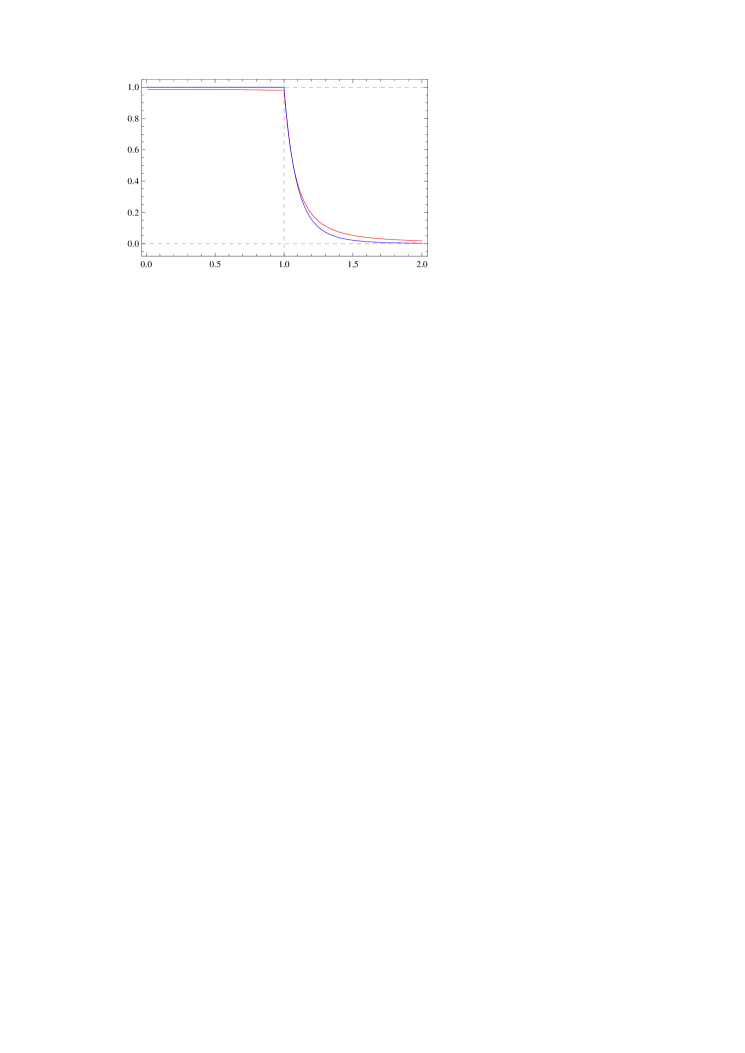
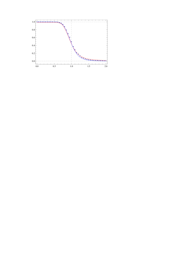
Figure 1. ​(Exponential $Y$–Exponential $T$)  Graphs ($X$-axis is $c$) of the functions $\mathsf{P}\{v<\Upsilon\leqslant t\mid T_{1}=v\}$ (blue) given in Theorem 3.1 and ${\mathcal{M}}_{t}(u,c,v)$ (red) for Exponential $T$ with parameter $\beta$ and Exponential $Y$ with parameter $\alpha$, as $\beta=\alpha=1$, $v=0$, $u=10$, $t=\infty$ (above), $t=100$ (below). By dots, shown are the results of simulation ($\Delta c=0.05$, $N=1000$) according to the algorithm described in Section 4.3.

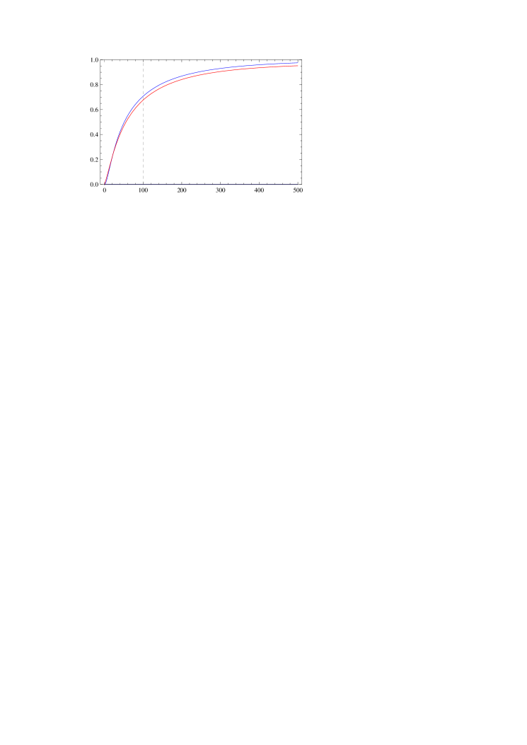
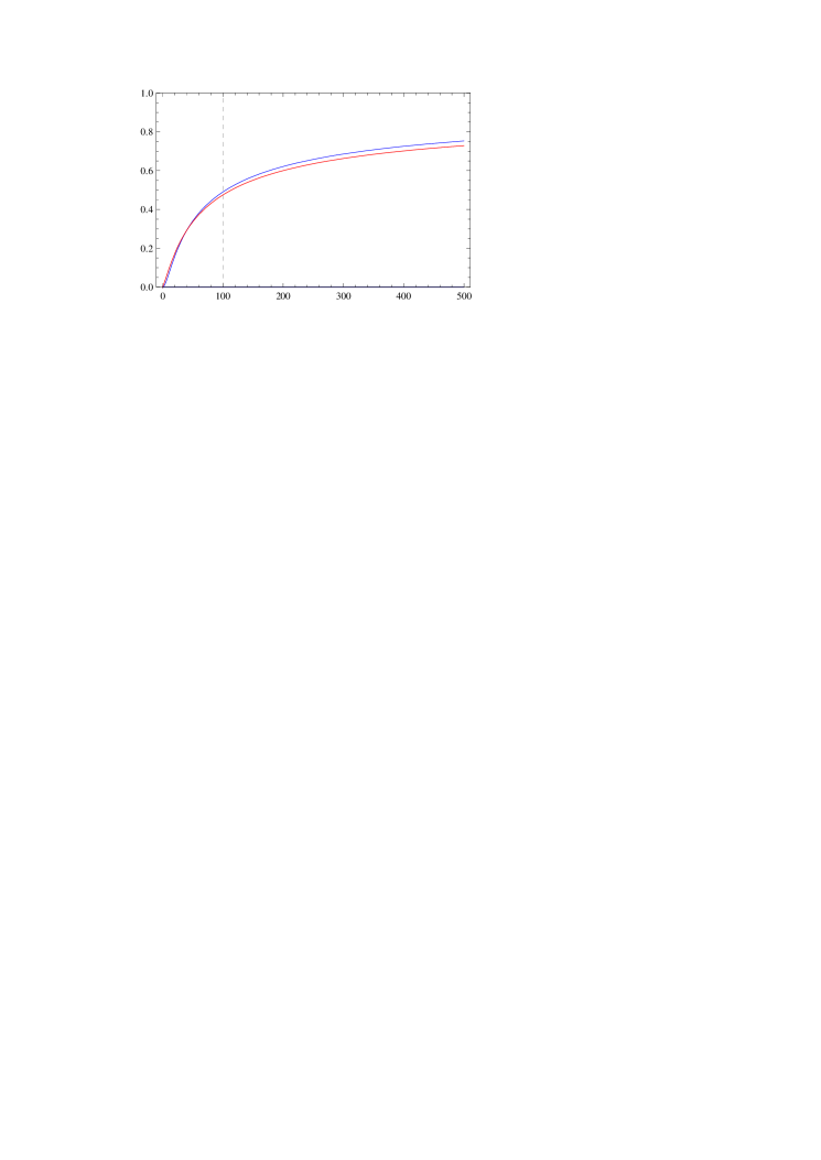
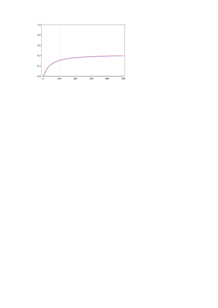
Figure 2. ​(Exponential $Y$–Exponential $T$)  Graphs ($X$-axis is $t$) of the functions $\mathsf{P}\{v<\Upsilon\leqslant t\mid T_{1}=v\}$ (blue) given in Theorem 3.1 and ${\mathcal{M}}_{t}(u,c,v)$ (red) for Exponential $T$ with parameter $\beta$ and Exponential $Y$ with parameter $\alpha$, as $\beta=\alpha=1$, $v=0$, $u=10$, $c=0.9$ (above), $c=1$ (middle), $c=1.1$ (below).

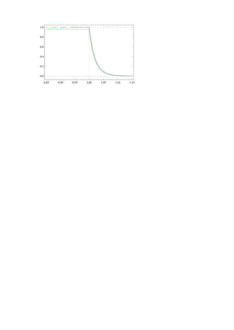
Figure 3. ​(Exponential $Y$–Exponential $T$)  Graphs ($X$-axis is $c$) of the functions $\mathsf{P}\{v<\Upsilon\leqslant t\mid T_{1}=v\}$ (blue) given in Theorem 3.1 and $\mathcal{E}_{t}(u,c,v)$ (green) defined in equation (2.1), for Exponential $T$ with parameter $\beta$ and Exponential $Y$ with parameter $\alpha$, as $\beta=\alpha=1$, $v=0$, $u=50$, $t=\infty$ (above), $t=1000$ (below). By dots, shown are the results of simulation ($\Delta c=0.01$, $N=1000$) according to the algorithm described in Section 4.3.

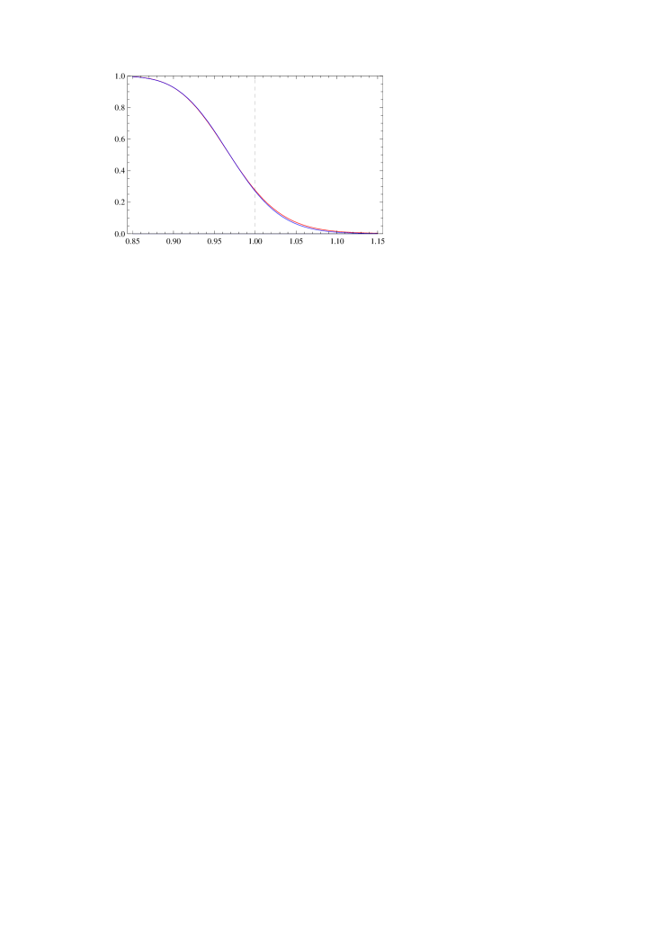
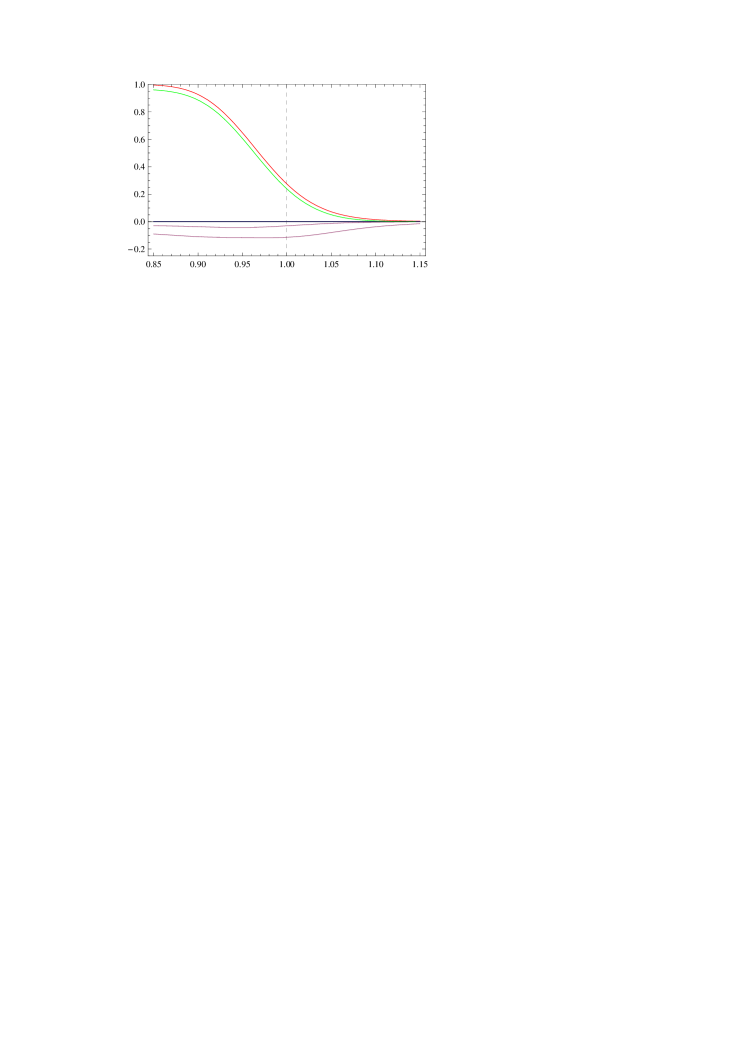
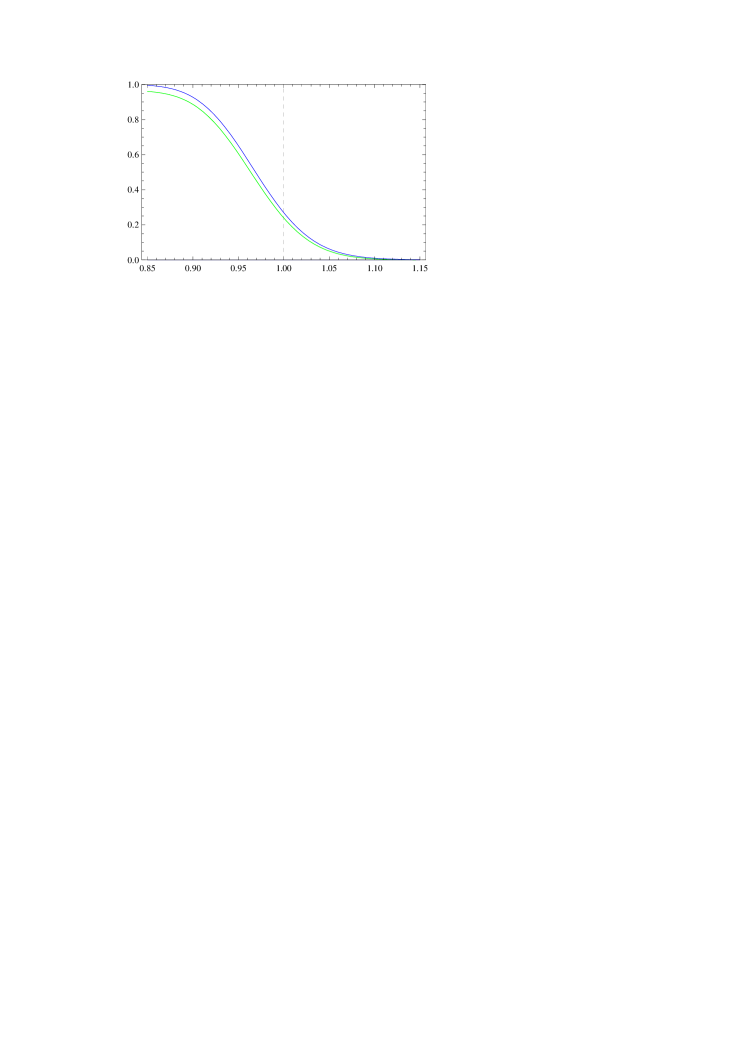
Figure 4. ​(Exponential $Y$–Exponential $T$)  Above: graphs ($X$-axis is $c$) of the functions $\mathsf{P}\{v<\Upsilon\leqslant t\mid T_{1}=v\}$ (blue) given in Theorem 3.1 and ${\mathcal{M}}_{t}(u,c,v)$ (red). Middle: graphs of ${\mathcal{M}}_{t}(u,c,v)$ (red), $\mathcal{E}_{t}(u,c,v)$ (green), ${\mathcal{F}}_{t}(u,c,v)$, and ${\mathcal{S}}_{t}(u,c,v)$. Below: graphs of $\mathsf{P}\{v<\Upsilon\leqslant t\mid T_{1}=v\}$ (blue) and $\mathcal{E}_{t}(u,c,v)$ (green). Here $\beta=\alpha=1$, $t=1000$, $v=0$, $u=50$. In this case, $c^{*}=1/M=1$, $D^{2}=2$, $C_{\mathcal{F}}\,=0.25\,c^{-1}$, $C_{\mathcal{F}}\,=0.25\,c^{-1}$.

Let us consider the case when $T$ is Exponential with parameter $\beta>0$ and $Y$ is Exponential with parameter $\alpha>0$. Plainly,

$$\mathsf{E}{T}=\frac{1}{\beta},\quad\mathsf{D}{T}=\frac{1}{\beta^{2}},\quad\mathsf{E}{Y}=\frac{1}{\alpha},\quad\mathsf{D}{Y}=\frac{1}{\alpha^{2}},$$

and

$$M=\frac{\alpha}{\beta},\quad D^{2}=\frac{2\alpha}{\beta^{2}}.$$

It is calculated straightforwardly that

$$C_{\mathcal{F}}\,=\frac{\beta}{4\alpha\,c},\quad C_{\mathcal{S}}\,=\frac{\beta}{4\alpha\,c}.$$

Denote by $I_{\nu}(z)$ the modified Bessel function of the first kind of order $\nu$ (see, e.g., [Abramowitz Stegun 1972]). For $T$ and $Y$ Exponential, one can get an exact formula for $\mathsf{P}\{v<\Upsilon\leqslant t\mid T_{1}=v\}$ as follows.

Theorem 3.1.

Assuming that $T$ and $Y$ are Exponential with parameters $\beta>0$ and $\alpha>0$ respectively, for $0<v<t$ we have

$$\mathsf{P}\{v<\Upsilon\leqslant t\mid T_{1}=v\}=\sqrt{\alpha\beta c}\,(v+u/c)e^{-\alpha u}e^{-\alpha cv}\\ \times\int_{0}^{t-v}\frac{I_{1}(2\sqrt{\alpha\beta c(y+v+u/c)y})}{\sqrt{(y+v+u/c)y}}e^{-(\alpha c+\beta)y}dy.$$

Proof of Theorem 3.1.

For $M(s)=\inf\big{\{}k\geqslant 1:\sum_{i=1}^{k}Y_{i}>s\big{\}}-1$ and $0<v<t$, we have (see equation (2.1) in [Malinovskii 2017a])

$$\mathsf{P}\{v<\Upsilon\leqslant t\mid T_{1}=v\}=\int_{v}^{t}\dfrac{u+cv}{u+cz}\sum_{n=1}^{\infty}\mathsf{P}\{M(u+cz)=n\}f_{T}^{*n}(z-v)dz.$$ (3.1)

For $T$ Exponential with parameter $\beta$, we have

$$f_{T}^{*n}(z-v)=\beta\frac{(\beta(z-v))^{n-1}}{(n-1)!}e^{-\beta(z-v)},\quad n=1,2,\dots.$$ (3.2)

For $Y$ Exponential with parameter $\alpha$, we have

$$\mathsf{P}\{M(u+cz)=n\}=\frac{(\alpha(u+cz))^{n}}{n!}e^{-\alpha(u+cz)},\quad n=1,2,\dots.$$ (3.3)

Bearing in mind that modified Bessel function of the first kind of order $1$ is

$$I_{1}(z)=\sum_{k=0}^{\infty}\frac{1}{k!\,(k+1)!}\left(\frac{z}{2}\right)^{2k+1}=\sum_{n=1}^{\infty}\frac{1}{n!\,(n-1)!}\left(\frac{z}{2}\right)^{2n-1},$$

we put (3.2) and (3.3) in (3.1). We have

$$\int_{v}^{t}\frac{u+cv}{u+cz}e^{-\alpha(u+cz)}\sum_{n=1}^{\infty}\frac{(\alpha(u+cz))^{n}}{n!}\beta\frac{(\beta(z-v))^{n-1}}{(n-1)!}e^{-\beta(z-v)}dz\\ =\alpha\beta\int_{v}^{t}(u+cv)\sum_{n=1}^{\infty}\frac{\alpha^{n-1}\beta^{n-1}(u+cz)^{n-1}(z-v)^{n-1}}{n!(n-1)!}e^{-\alpha(u+cz)}e^{-\beta(z-v)}dz\\ =\sqrt{\alpha\beta c}\,(v+u/c)e^{-\alpha u}e^{-\alpha cv}\int_{0}^{t-v}\frac{I_{1}(2\sqrt{\alpha\beta c(y+v+u/c)y})}{\sqrt{(y+v+u/c)y}}e^{-(\alpha c+\beta)y}dy,$$

as required. In the last equation we made the change of variables: $z-v=y$. ∎

In Figs. 1–4, performance of the approximations ${\mathcal{M}}_{t}(u,c,v)$, $\mathcal{E}_{t}(u,c,v)$ of Theorems 2.1 and 2.2 is visualized, when $T$ is Exponential with parameter $\beta=1$ and $Y$ is Exponential with parameter $\alpha=1$.

In Figs. 1 and 3 respectively, we compare ${\mathcal{M}}_{t}(u,c,v)$ and $\mathcal{E}_{t}(u,c,v)$ with the exact numerical values for $\mathsf{P}\{v<\Upsilon\leqslant t\mid T_{1}=v\}$ given in Theorem 3.1, as $c$ varies and $t$ is fixed. The results of simulation according to the algorithm described in Section 4.3, are shown by dots. In Fig. 2, it is done, as $t$ varies and $c$ is fixed. Figs. 1–3 demonstrate good accuracy of both approximations ${\mathcal{M}}_{t}(u,c,v)$ and $\mathcal{E}_{t}(u,c,v)$ throughout all chosen range of $c$ and $t$.

In Fig. 4, visualized is performance of the approximation ${\mathcal{M}}_{t}(u,c,v)$ of Theorem 2.1 (above), and of the approximation $\mathcal{E}_{t}(u,c,v)$ of Theorem 2.2 (below); both are compared with the exact numerical values for $\mathsf{P}\{v<\Upsilon\leqslant t\mid T_{1}=v\}$ given in Theorem 3.1. On the one hand, it may be seen that in this test case the former lies closer to the exact than the latter. On the other hand, the latter lies consistently below the exact all over $c$ in all range chosen, while the latter does not. Visualization is also done (middle) for the components ${\mathcal{F}}_{t}(u,c,v)$ and ${\mathcal{S}}_{t}(u,c,v)$ which, together with the factors $C_{\mathcal{F}}\,$ and $C_{\mathcal{S}}\,$, produce $\mathcal{E}_{t}(u,c,v)$ as in (2.1). It is noteworthy that lower Fig. 3 and lower Fig. 4 are the same, except that simulation results are shown on the former.

4. Performance of approximations when $T$ and $Y$ are non-Exponential

First, we recall the properties of three non-Exponential distributions which will be selected as distributions of $T$ and $Y$. Second, we describe the algorithm of numerical simulation. Finally, we present the main results of this section.

4.1. Three non-Exponential distributions

Let us select the Mixture of two Exponentials and Erlang distributions as two non-Exponential distributions which properties strongly resemble those of Exponential, and Pareto, which properties are far from those of Exponential; in particular, it is well known that Pareto is heavy-tailed.

Case 4.1 (Mixture of two Exponentials).

The random variable $X$ is a Mixture of two Exponentials if for $0<\lambda_{1}<\lambda_{2}<\infty$ and for $p$, $q$ such that $p+q=1$, $0\leqslant p,q\leqslant 1$, its p.d.f. is

$$f_{X}(x)=\lambda_{1}pe^{-\lambda_{1}x}+\lambda_{2}qe^{-\lambda_{2}x},\quad x>0,$$

and $0$, as $x\leqslant 0$. Plainly, the corresponding c.d.f. $F_{X}(x)=\int_{0}^{x}f_{X}(z)dz$ is

$$F_{X}(x)=1-(pe^{-\lambda_{1}x}+qe^{-\lambda_{2}x}),\quad x>0,$$ (4.1)

and $0$, as $x\leqslant 0$. By direct calculations, it is easy to check that

$$\begin{gathered}\mathsf{E}{X}=\frac{p}{\lambda_{1}}+\frac{q}{\lambda_{2}},\quad\mathsf{D}{X}=\frac{q\lambda_{1}^{2}+p\lambda_{2}^{2}+pq(\lambda_{1}-\lambda_{2})^{2}}{\lambda_{1}^{2}\lambda_{2}^{2}},\quad\\[6.0pt] \mathsf{E}(X-\mathsf{E}{X})^{3}=-\frac{6pq^{2}}{\lambda_{1}^{2}\lambda_{2}}-\frac{6p^{2}q}{\lambda_{1}\lambda_{2}^{2}}+\frac{2p\big{(}3q+p^{2}\big{)}}{\lambda_{1}^{3}}+\frac{2q\big{(}3p+q^{2}\big{)}}{\lambda_{2}^{3}}.\end{gathered}$$

Case 4.2 (Erlang).

The random variable $X$ is Erlang if for $\theta>0$ and integer $k$ its p.d.f. is

$$f_{X}(x)=\frac{\theta^{k}x^{k-1}}{\Gamma(k)}e^{-x\theta},\quad x>0,$$

and $0$, as $x\leqslant 0$. It is well known that Erlang is a particular case of the Gamma p.d.f.

By direct calculations, it is easy to check that

$$\mathsf{E}{X}=\frac{k}{\theta},\quad\mathsf{D}{X}=\frac{k}{\theta^{2}},\quad\mathsf{E}(X-\mathsf{E}{X})^{3}=\frac{2k}{\theta^{3}}.$$

Case 4.3 (Pareto).

The random variable $X$ is Pareto if for $a>0$ and $b>0$ its p.d.f. is

$$f_{X}(x)=\dfrac{ab}{(xb+1)^{a+1}},\quad x>0,$$

and $0$, as $x\leqslant 0$. Plainly, the corresponding c.d.f. $F_{X}(x)=\int_{0}^{x}f_{X}(z)dz$ is

$$F_{X}(x)=1-\frac{1}{(xb+1)^{a}},\quad x>0,$$ (4.2)

and $0$, as $x\leqslant 0$. By direct calculations, it is easy to check that for $a>3$ we have

$$\mathsf{E}{X}=\frac{1}{(a-1)\,b},\quad\mathsf{D}{X}=\frac{a}{(a-1)^{2}(a-2)\,b^{2}},\quad\mathsf{E}(X-\mathsf{E}{X})^{3}=\frac{2a(a+1)}{(a-1)^{3}(a-2)(a-3)\,b^{3}}.$$

4.2. Algorithm of simulation

The starting point for the entire simulation process is a pseudo-random number generator from Uniform [0,1] distribution. We deal with the standard (see [Knuth 1981]) linear congruence random number generator based on the equation

$$x_{n+1}=(\kappa x_{n}+\varrho)\ \mod\ m,$$

where $\kappa=23456789$ is the multiplier, $\varrho=22185$ is the increment, and $m=2^{32}$ is the modulus. The initial seed $x_{0}$ is selected using a build-in Maple procedure. Each successive term is transformed into the next. The pseudo-random terms are in the range from $1$ to $m-1$. To get floating point numbers between $0$ and $1$, a floating point division by $m$ is done. It is known that matching of the numbers thus produced to a sample from the Uniform $[0,1]$ distribution depends heavily on the choice of $\kappa$ and $m$.

Using this pseudo-random number generator from Uniform [0,1] distribution, pseudo-random numbers from Exponential, Mixture of two Exponentials, Erlang, and Pareto distributions are all obtained using the method of inverse transforms (see, e.g., [Devroye 1986]). For instance, pseudo-random number from Mixture of two Exponentials is $E=F^{-1}_{X}(U)$ with c.d.f. $F_{X}$ given in (4.1), or for $\lambda_{1}=1$ and $\lambda_{2}=2$ in explicit form

$$E=-\ln\bigg{(}\frac{-p+\sqrt{p^{2}+4q(1-U)}}{2q}\bigg{)},$$ (4.3)

and pseudo-random number from Pareto is $P=F^{-1}_{X}(U)$ with c.d.f. $F_{X}$ given in (4.2), or in explicit form

$$P=\frac{1}{b}\bigg{(}\frac{1}{(1-U)^{1/a}}-1\bigg{)},$$ (4.4)

where $U$ is pseudo-random number from Uniform $[0,1]$ distribution produced by the generator described above.

To evaluate, using numerical simulation, the probability $\mathsf{P}\{v<\Upsilon\leqslant t\mid T_{1}=v\}$ as a function of $c$, while $u$, $t$, $v$ are fixed, we address the interval $[c_{\min},c_{\max}]$ on the abscissa axis, where $c^{*}=1/M\in[c_{\min},c_{\max}]$. We introduce the lattice

$$\mathcal{C}=\{c_{i},\ i=0,1,\dots,n_{\mathcal{C}}\}$$

with the span $\Delta c>0$, i.e. put $c_{0}=0$ and $c_{i}=c_{i-1}+\Delta c$, $i=1,2,\dots,[c_{\max}/\Delta c]+1$.

Starting with $c_{0}$, we iterate through the nodes of $\mathcal{C}$. Dealing with the node $c_{i}$, we simulate the values $\mathsf{P}\{v<\Upsilon\leqslant t\mid T_{1}=v\}$ at the points $c_{i}$, $i=0,1,\dots,n_{\mathcal{C}}$ on the basis of the definition of this probability. Namely, for each $c_{i}$ we simulate the bundle consisting of $N$ trajectories of the process $V_{s}-c_{i}s$. Then we pick up the ratio of the trajectories that crossed the level $u$ to the total number of trajectories $N$ and declare it the value of the probability in question in the node $c_{i}$.

4.3. Approximations and simulation results

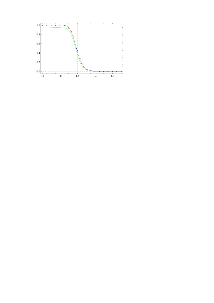
Figure 5. ​(Erlang $Y$–Erlang $T$)  Above: graphs ($X$-axis is $c$) of the functions ${\mathcal{M}}_{t}(u,c,v)$ (red), ${\mathcal{F}}_{t}(u,c,v)$, ${\mathcal{S}}_{t}(u,c,v)$; below: graphs of the functions ${\mathcal{M}}_{t}(u,c,v)$ (red), $\mathcal{E}_{t}(u,c,v)$ (green) in the case when $Y$ is Erlang with parameters $\alpha=1$, $m=2$, $T$ is Erlang with parameters $\beta=1.2$, $k=2$, and $t=1000$, $v=0$, $u=40$. In this case, $c^{*}=1/M=1.2$, $D^{2}=1.39$, $C_{\mathcal{F}}\,=0.6\,c^{-1}$, $C_{\mathcal{S}}\,=0.3\,c^{-1}$. By dots, shown are the results of simulation ($\Delta c=0.05$, $N=1000$) according to the algorithm described in Section 4.3.

The following Lemma 4.1 is applied to calculate approximations ${\mathcal{M}}_{t}(u,c,v)$ and $\mathcal{E}_{t}(u,c,v)$ for Erlang $Y$ and $T$, shown in Fig. 5.

Lemma 4.1 (Erlang $Y$–Erlang $T$).

For $Y$ Erlang with parameters $\alpha>0$ and integer $m$, and $T$ Erlang with parameters $\beta>0$ and integer $k$, i.e., for

$$f_{Y}(x)=\frac{\alpha^{m}x^{m-1}}{\Gamma(m)}\,e^{-x\alpha},\quad f_{T}(x)=\frac{\beta^{k}x^{k-1}}{\Gamma(k)}\,e^{-x\beta},\quad x>0,$$

and $0$, as $x\leqslant 0$, we have

$$M=\frac{\alpha k}{\beta m},\quad D^{2}=\frac{\alpha k(k+m)}{m^{2}\beta^{2}},\quad C_{\mathcal{F}}\,=\frac{\beta m((2+m)k-2m)}{2\alpha k(k+m)\,c},\quad C_{\mathcal{S}}\,=\frac{\beta m(k+2m)}{6\alpha k(k+m)\,c}.$$

The following corollary is straightforward, if we put $m=1$.

Corollary 4.1 (Exponential $Y$–Erlang $T$).

For $Y$ Exponential with parameter $\alpha>0$, and $T$ Erlang with parameters $\beta>0$ and integer $k$, we have

$$M=\frac{\alpha k}{\beta},\quad D^{2}=\frac{\alpha k(k+1)}{\beta^{2}},\quad C_{\mathcal{F}}\,=\frac{\beta(3k-2)}{2\alpha k(k+1)\,c},\quad C_{\mathcal{S}}\,=\frac{\beta(k+2)}{6\alpha k(k+1)\,c}.$$

In upper and lower Fig. 5, in the case when $Y$ is Erlang with parameters $\alpha=1$, $m=2$, $T$ is Erlang with parameters $\beta=1.2$, $k=2$, and $t=1000$, $v=0$, $u=40$, visualized are the functions ${\mathcal{M}}_{t}(u,c,v)$, ${\mathcal{F}}_{t}(u,c,v)$, ${\mathcal{S}}_{t}(u,c,v)$ which, together with the factors $C_{\mathcal{F}}\,=0.6\,c^{-1}$, $C_{\mathcal{S}}\,=0.3\,c^{-1}$, are involved (see (2.1)) in the construction of $\mathcal{E}_{t}(u,c,v)$. Visualized are also the approximations ${\mathcal{M}}_{t}(u,c,v)$ and $\mathcal{E}_{t}(u,c,v)$, compared with the results of simulation shown by dots. The simulation algorithm is described in Section 4.3 ($\Delta c=0.05$ and more frequent in the flexure region, $N=1000$). Simulation demonstrates that in this test case ${\mathcal{M}}_{t}(u,c,v)$ looks preferable for $c<c^{*}$, though both ${\mathcal{M}}_{t}(u,c,v)$ and $\mathcal{E}_{t}(u,c,v)$ look equally accurate for $c>c^{*}$.

The following Lemma 4.2 is applied to calculate approximations ${\mathcal{M}}_{t}(u,c,v)$ and $\mathcal{E}_{t}(u,c,v)$ in the case of Pareto $Y$ and Mixture of two Exponentials $T$, shown in Fig. 6.

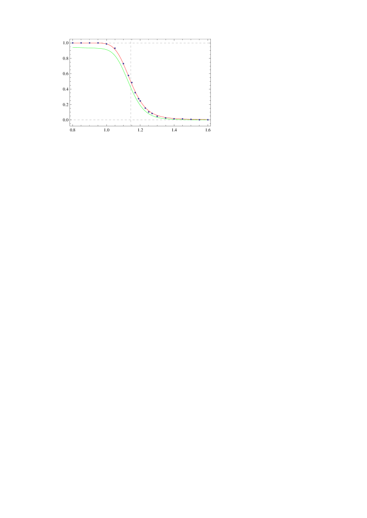
Figure 6. ​(Pareto $Y$–Mixture of two Exponentials $T$)  Above: graphs ($X$-axis is $c$) of the functions ${\mathcal{M}}_{t}(u,c,v)$ (red), ${\mathcal{F}}_{t}(u,c,v)$, ${\mathcal{S}}_{t}(u,c,v)$; below: graphs of the functions ${\mathcal{M}}_{t}(u,c,v)$ (red), $\mathcal{E}_{t}(u,c,v)$ (green) in the case when $Y$ is Pareto with parameters $a_{Y}=4.0$, $b_{Y}=0.35$, $T$ is Mixture of two Exponentials with parameters $\lambda_{1}=1$, $\lambda_{2}=2$, $p=2/3$, and $t=1000$, $v=0$, $u=40$. In this case, $c^{*}=1/M=1.143$, $D^{2}=2.304$, $C_{\mathcal{F}}\,=1.04\,c^{-1}$, $C_{\mathcal{S}}\,=0.076\,c^{-1}$. By dots, shown are the results of simulation ($\Delta c=0.05$, $N=1000$) according to the algorithm described in Section 4.3.

Lemma 4.2 (Pareto $Y$–Mixture of two Exponentials $T$).

For $Y$ Pareto with parameters $a_{Y}>3$, $b_{Y}>0$, and $T$ Mixture of two Exponentials with parameters $\lambda_{1}>0$, $\lambda_{2}>0$, and $0<p<1$ ($q=1-p$), i.e., for

$$f_{Y}(x)=\dfrac{a_{Y}b_{Y}}{(xb_{Y}+1)^{a_{Y}+1}},\quad f_{T}(x)=\lambda_{1}pe^{-\lambda_{1}x}+\lambda_{2}qe^{-\lambda_{2}x},\quad x>0,$$

and $0$, as $x\leqslant 0$, we have

$$\begin{gathered}M=(a_{Y}-1)b_{Y}\bigg{(}\frac{p}{\lambda_{1}}+\frac{q}{\lambda_{2}}\bigg{)},\\[4.0pt] D^{2}=(a_{Y}-1)b_{Y}\bigg{(}\frac{a_{Y}}{a_{Y}-2}\Big{(}\frac{p}{\lambda_{1}}+\frac{q}{\lambda_{2}}\Big{)}^{2}+\frac{\lambda_{2}^{2}p+\lambda_{1}^{2}q+(\lambda_{1}-\lambda_{2})^{2}pq}{\lambda_{1}^{2}\lambda_{2}^{2}}\bigg{)},\end{gathered}$$

$$C_{\mathcal{F}}\,=\frac{(a_{Y}-2)\lambda_{1}\lambda_{2}}{2(a_{Y}-3)(a_{Y}-1)b_{Y}\,\big{(}4\lambda_{1}\lambda_{2}pq+2\lambda_{1}^{2}q(a_{Y}-(1+p))+2\lambda_{2}^{2}p(a_{Y}-(1+q))\big{)}^{2}\,c}\\[4.0pt] \times\Big{(}\lambda_{2}^{3}\big{(}(-12+9a_{Y}+a_{Y}^{2})p^{3}-12(6-5a_{Y}+a_{Y}^{2})pq-2(6-5a_{Y}+a_{Y}^{2})q^{3}\\ +(6-5a_{Y}+a_{Y}^{2})p^{2}(1+q)\big{)}+\lambda_{1}^{3}q^{2}\big{(}6(1+p)-a_{Y}(6+4p)+a_{Y}^{2}(1+p+3q)\big{)}\\ +\lambda_{1}\lambda_{2}^{2}pq\big{(}6-12p+a_{Y}(-5+7p-35q)+42q+a_{Y}^{2}(1+7p+7q)\big{)}\\ +\lambda_{1}^{2}\lambda_{2}pq\big{(}6(1+7p-2q)+a_{Y}(-5-35p+7q)+a_{Y}^{2}(1+7p+7q)\big{)}\Big{)},$$

$$C_{\mathcal{S}}\,=\frac{(a_{Y}-2)^{2}\lambda_{1}\lambda_{2}^{4}}{6(a_{Y}-1)b_{Y}(4\lambda_{1}\lambda_{2}pq+2\lambda_{1}^{2}q(a_{Y}-(1+p))+4\lambda_{2}^{2}p(a_{Y}-(1+q)))^{2}\,c}\\[4.0pt] \times\bigg{(}-\frac{6\lambda_{1}^{2}p^{2}q}{\lambda_{2}^{2}}-\frac{6\lambda_{1}pq^{2}}{\lambda_{2}}+2p(p^{2}+3q)-\frac{2a_{Y}(1+a_{Y})(\lambda_{2}p+\lambda_{1}q)^{3}}{(6-5a_{Y}+a_{Y}^{2})\lambda_{2}^{3}}+2q(3p+q^{2})\\[-2.0pt] +\frac{3a_{Y}(\lambda_{2}p+\lambda_{1}q)}{(a_{Y}-2)^{2}\lambda_{2}^{3}}\Big{(}4\lambda_{1}\lambda_{2}pq+2\lambda_{1}^{2}q\big{(}a_{Y}-(1+p)\big{)}+2\lambda_{2}^{2}p\big{(}a_{Y}-(1+q)\big{)}\Big{)}\bigg{)}.$$

In Fig. 6, visualization is done in the case when $Y$ is Pareto with parameters $a_{Y}=4.0$, $b_{Y}=0.35$, and $T$ is Mixture of two Exponentials with parameters $\lambda_{1}=1$, $\lambda_{2}=2$, $p=2/3$, and $t=1000$, $v=0$, $u=40$. Simulation is done according to the algorithm described in Section 4.3 ($\Delta c=0.05$ and more frequent in the flexure region, $N=1000$), using equation (4.4) for Pareto $Y$ and equation (4.3) for Mixture of two Exponentials $T$ with $\lambda_{1}=1$ and $\lambda_{2}=2$.

The following Lemma 4.3 is applied to calculate approximations ${\mathcal{M}}_{t}(u,c,v)$ and $\mathcal{E}_{t}(u,c,v)$ for Pareto $Y$ and Erlang $T$, shown in Fig. 7.

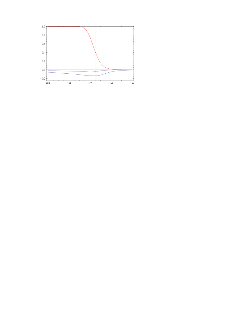
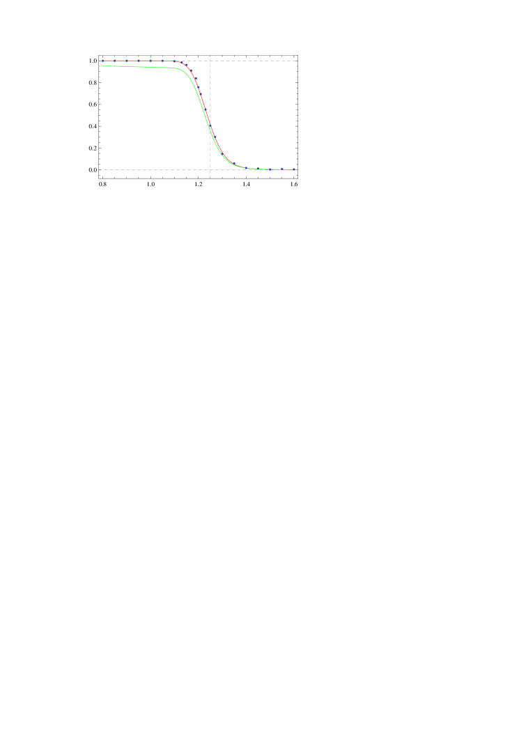
Figure 7. ​(Pareto $Y$–Erlang $T$)  Above: graphs ($X$-axis is $c$) of the functions ${\mathcal{M}}_{t}(u,c,v)$ (red), ${\mathcal{F}}_{t}(u,c,v)$, ${\mathcal{S}}_{t}(u,c,v)$; below: graphs of the functions ${\mathcal{M}}_{t}(u,c,v)$ (red), $\mathcal{E}_{t}(u,c,v)$ (green) in the case when $Y$ is Pareto with parameters $a_{Y}=4.0$, $b_{Y}=0.4$, $T$ is Erlang with parameters $\beta=6.0$, $k=4$, and $t=1000$, $v=0$, $u=40$. In this case, $c^{*}=1/M=1.25$, $D^{2}=1.2$, $C_{\mathcal{F}}\,=2.73\,c^{-1}$, $C_{\mathcal{S}}\,=-0.26\,c^{-1}$. By dots, shown are the results of simulation ($\Delta c=0.05$, $N=1000$) according to the algorithm described in Section 4.3.

Lemma 4.3 (Pareto $Y$–Erlang $T$).

For $Y$ Pareto with parameters $a_{Y}>3$, $b_{Y}>0$, and $T$ Erlang with parameters $\beta>0$ and integer $k$, i.e., for

$$f_{Y}(x)=\dfrac{a_{Y}b_{Y}}{(xb_{Y}+1)^{a_{Y}+1}},\quad f_{T}(x)=\frac{\beta^{k}x^{k-1}}{\Gamma(k)}e^{-x\beta},\quad x>0,$$

and $0$, as $x\leqslant 0$, we have

$$M=\frac{k(a_{Y}-1)b_{Y}}{\beta},\quad D^{2}=\frac{k(a_{Y}-1)b_{Y}}{\beta^{2}}\bigg{(}1+\frac{ka_{Y}}{a_{Y}-2}\bigg{)},$$

$$\begin{gathered}C_{\mathcal{F}}\,=(a_{Y}-2)\beta\,\frac{a_{Y}^{2}(-2+k+3k^{2})-a_{Y}(-10+5k+k^{2})+6(-2+k)}{2(a_{Y}-1)(a_{Y}-3)b_{Y}k(-2+a_{Y}+a_{Y}k)^{2}\,c},\\[4.0pt] C_{\mathcal{S}}\,=\beta\,\frac{a_{Y}^{3}(2+3k+k^{2})-a_{Y}^{2}(14+15k+7k^{2})+2a_{Y}(16+9k+2k^{2})-24}{6(a_{Y}-1)(a_{Y}-3)b_{Y}k(-2+a_{Y}+a_{Y}k)^{2}\,c}.\end{gathered}$$

In Fig. 7, visualized is the case when $Y$ is Pareto with parameters $a_{Y}=4.0$, $b_{Y}=0.4$, $T$ is Erlang with parameters $\beta=6.0$, $k=4$, and $t=1000$, $v=0$, $u=40$. Simulation is done according to the algorithm described in Section 4.3 ($\Delta c=0.05$ and more frequent in the flexure region, $N=1000$), using equation (4.4) and bearing in mind that this Erlang $T$ is a sum of four i.i.d. Exponential summands with parameter $\beta=6.0$.

The following Lemma 4.4 is applied to calculate approximations ${\mathcal{M}}_{t}(u,c,v)$ and $\mathcal{E}_{t}(u,c,v)$ for Pareto $Y$ and $T$, shown in Fig. 8.

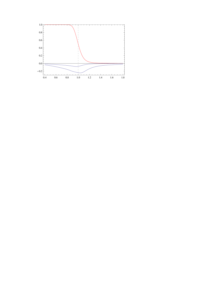
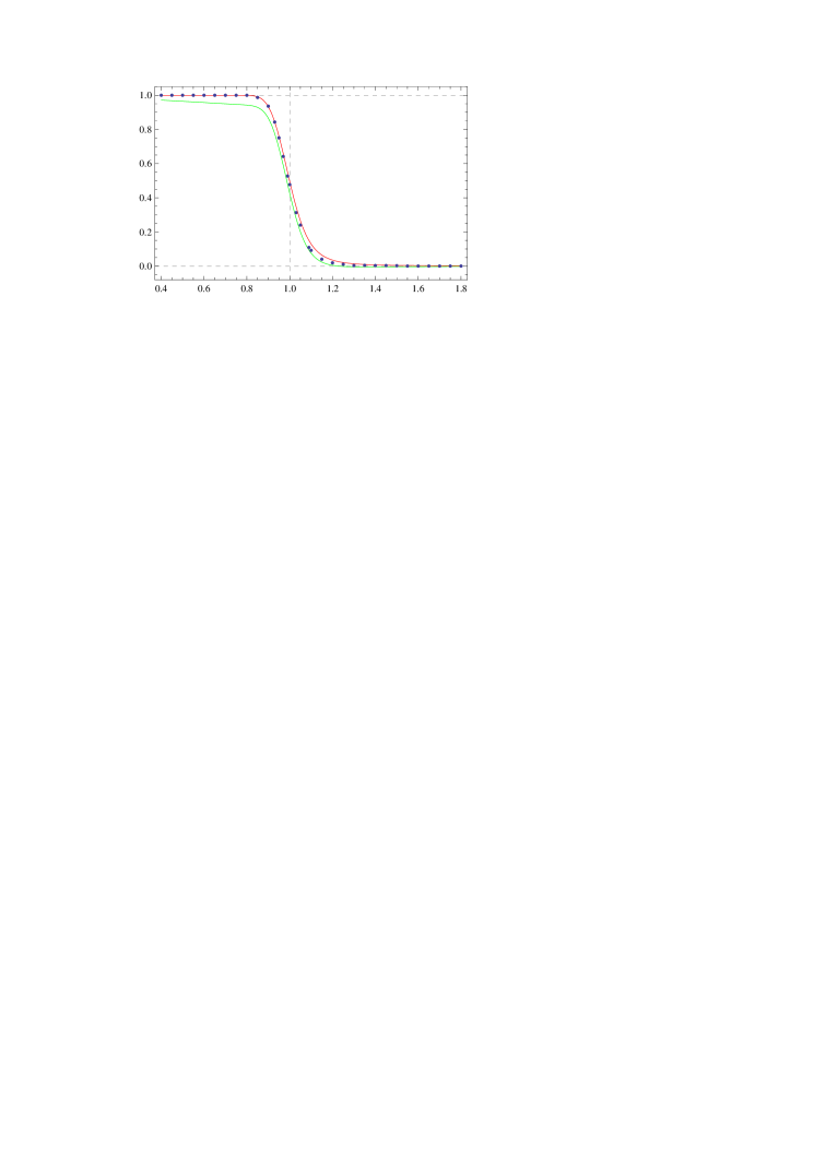
Figure 8. ​(Pareto $Y$–Pareto $T$)  Above: graphs ($X$-axis is $c$) of the functions ${\mathcal{M}}_{t}(u,c,v)$ (red), ${\mathcal{F}}_{t}(u,c,v)$, ${\mathcal{S}}_{t}(u,c,v)$; below: graphs of the functions ${\mathcal{M}}_{t}(u,c,v)$ (red), $\mathcal{E}_{t}(u,c,v)$ (green) in the case when $T$ is Pareto with parameters $a_{T}=4.0$, $b_{T}=0.4$, $Y$ is Pareto with parameters $a_{Y}=4.0$, $b_{Y}=0.4$, and $t=1000$, $v=0$, $u=40$. In this case, $c^{*}=1/M=1$, $D^{2}=3.333$, $C_{\mathcal{F}}\,=0.125\,c^{-1}$, $C_{\mathcal{S}}\,=0.25\,c^{-1}$. By dots, shown are the results of simulation ($\Delta c=0.05$, $N=1000$) according to the algorithm described in Section 4.3.

Lemma 4.4 (Pareto $Y$–Pareto $T$).

For $Y$ Pareto with parameters $a_{Y}>3$, $b_{Y}>0$, and $T$ Pareto with parameters $a_{T}>3$, $b_{T}>0$, i.e., for

$$f_{Y}(x)=\dfrac{a_{Y}b_{Y}}{(xb_{Y}+1)^{a_{Y}+1}},\quad f_{T}(x)=\dfrac{a_{T}b_{T}}{(xb_{T}+1)^{a_{T}+1}},\quad x>0,$$

and $0$, as $x\leqslant 0$, we have

$$M=\frac{(a_{Y}-1)b_{Y}}{(a_{T}-1)b_{T}},\quad D^{2}=\bigg{(}\frac{a_{Y}}{a_{Y}-2}+\frac{a_{T}}{a_{T}-2}\bigg{)}\frac{(a_{Y}-1)b_{Y}}{(a_{T}-1)^{2}b_{T}^{2}},$$

$$C_{\mathcal{F}}\,=\frac{(a_{T}-2)(a_{Y}-2)b_{T}}{4(a_{T}-3)(a_{Y}-3)b_{Y}}\\[4.0pt] \times\frac{a_{Y}^{2}(9-10a_{T}+a_{T}^{2})+a_{Y}(-3+15a_{T}+2a_{T}^{2})-3a_{T}(5+a_{T})}{(a_{Y}-1)^{3}(a_{T}-1)\,c},$$

$$C_{\mathcal{S}}\,=\frac{(a_{T}-2)b_{T}}{4(a_{T}-3)(a_{Y}-3)b_{Y}}\\[4.0pt] \times\frac{a_{Y}^{3}(a_{T}-1)^{2}-4a_{T}(1+a_{T})+a_{Y}^{2}(-7+11a_{T}-6a_{T}^{2})+a_{Y}(4-7a_{T}+9a_{T}^{2})}{(a_{Y}-1)^{3}(a_{T}-1)\,c}.$$

In Fig. 8, visualized are the functions ${\mathcal{M}}_{t}(u,c,v)$, ${\mathcal{F}}_{t}(u,c,v)$, ${\mathcal{S}}_{t}(u,c,v)$ which together with the factors $C_{\mathcal{F}}\,=0.125\,c^{-1}$, $C_{\mathcal{S}}\,=0.25\,c^{-1}$ are involved (see (2.1)) in the construction of $\mathcal{E}_{t}(u,c,v)$, and the approximations ${\mathcal{M}}_{t}(u,c,v)$, $\mathcal{E}_{t}(u,c,v)$ in the case when $T$ is Pareto with parameters $a_{T}=4.0$, $b_{T}=0.4$, $Y$ is Pareto with parameters $a_{Y}=4.0$, $b_{Y}=0.4$, and $t=1000$, $v=0$, $u=40$. By dots, shown are the results of simulation ($\Delta c=0.05$ and more frequent in the flexure region, $N=1000$) carried out according to the algorithm described in Section 4.3, using equation (4.4).

The comparison of ${\mathcal{M}}_{t}(u,c,v)$ and $\mathcal{E}_{t}(u,c,v)$ with the results of simulation shows that in all test cases of Figs. 5–8 both these approximations are surprisingly accurate, in particular in the vicinity of the point $c^{*}=1/M$, though $u=40$ chosen in Figs. 5–8 is rather moderate.

5. Conclusions

In the case of Exponential $T$ and $Y$, we have compared (a) numerical results yielded by approximations of Theorems 2.1 and 2.2, (b) numerical results derived by means of exact formula of Theorem 3.1, and (c) numerical results yielded by simulation. The availability of the exact formula in this case allows us, inter alia, to be confident in the error-free operating of the computer simulation program.

For $T$ and $Y$ non-Exponential, when exact formulas like in Theorems 3.1 do not exist or are excessively cumbersome (see, e.g., [Borovkov Dickson 2008]), in our hands remains only simulation technique. We use it for getting numerical benchmarks needed to verify and evaluate performance of the approximations ${\mathcal{M}}_{t}(u,c,v)$ and $\mathcal{E}_{t}(u,c,v)$ put forth in Theorems 2.1 and 2.2. The comparison of ${\mathcal{M}}_{t}(u,c,v)$ and $\mathcal{E}_{t}(u,c,v)$ and simulation results done in Section 4 indicates a good quality of these approximations.

It is noteworthy that the approximations ${\mathcal{M}}_{t}(u,c,v)$ and $\mathcal{E}_{t}(u,c,v)$, unlike, e.g., the famous Cramér-type approximation, hold true not only for the distributions of $Y$ with exponentially decreasing tail, but also for heavy-tailed $Y$, so we include Pareto distribution in our numerical analysis. Examining simulation results given in Figs. 1, 3, and 5–8, we see that the approximations ${\mathcal{M}}_{t}(u,c,v)$ and $\mathcal{E}_{t}(u,c,v)$ are very satisfactory for both light-tailed and heavy-tailed $T$ and $Y$. This examining confirms that the approximations ${\mathcal{M}}_{t}(u,c,v)$ and $\mathcal{E}_{t}(u,c,v)$ are satisfactory uniformly on $c$, including vicinity of the critical point $c^{*}=1/M$, in all cases considered. Generally, the accuracy of approximations ${\mathcal{M}}_{t}(u,c,v)$ and $\mathcal{E}_{t}(u,c,v)$ is visibly better than, e.g., of the Cramér-type approximation all over the range of $c$, including outside the vicinity of $c^{*}$; more detailed discussion of the deficiencies of Cramér-type approximation, from which ${\mathcal{M}}_{t}(u,c,v)$ and $\mathcal{E}_{t}(u,c,v)$ are free, may be seen in [Malinovskii Kosova 2014].

References

- [1]
- [Abramowitz and Stegun (1972)] Abramowitz, M., and Stegun, I.A. (1972) Handbook of Mathematical Functions, 10-th ed., Dover, New York.
- [Borovkov and Dickson (2008)] Borovkov, K., and Dickson, D.C.M. (2008) On the ruin time distribution for a Sparre Andersen process with exponential claim sizes, Insurance: Mathematics and Economics, Vol. 42, 1104–1108.
- [Devroye (1986)] Devroye, L. (1986) Non-uniform random variate generation. Springer-Verlag, New York.
- [Hellekalek (1998)] Hellekalek, P. (1998) Good random number generators are (not so) easy to find, Mathematics and Computers in Simulation, vol. 46, 485–505.
- [Knuth (1981)] Knuth, D.E. (1981) The Art of Computer Programming, Vol.2, Seminumerical Algorithms, 2nd ed., Addison Wesley.
- [Malinovskii (2017a)] Malinovskii, V.K. (2017a) On the time of first level crossing and inverse Gaussian distribution. Submitted.
- [Malinovskii (2017b)] Malinovskii, V.K. (2017b) Generalized inverse Gaussian distributions and the time of first level crossing. Submitted.
- [Malinovskii and Kosova (2014)] Malinovskii, V.K., and Kosova, K.O. (2014) Simulation analysis of ruin capital in Sparre Andersen’s model of risk, Insurance: Mathematics and Economics, Vol. 59, 184–193.
- [Watson (1945)] Watson, G.N. (1945) A Treatise on the Theory of Bessel Functions. Cambridge University Press, Cambridge.
- [Whittaker and Watson (1963)] Whittaker, E.T., and Watson, G.N. (1963) A Course of Modern Analysis. 4-th ed., Cambridge University Press, Cambridge.