Further Results on Size and Power of Heteroskedasticity and Autocorrelation Robust Tests, with an Application to Trend Testing

Abstract

We complement the theory developed in Preinerstorfer and Pötscher (2016) with further finite sample results on size and power of heteroskedasticity and autocorrelation robust tests. These allow us, in particular, to show that the sufficient conditions for the existence of size-controlling critical values recently obtained in Pötscher and Preinerstorfer (2018) are often also necessary. We furthermore apply the results obtained to tests for hypotheses on deterministic trends in stationary time series regressions, and find that many tests currently used are strongly size-distorted.

1 Introduction

Heteroskedasticity and autocorrelation robust tests in regression models suggested in the literature (e.g., tests based on the covariance estimators in Newey and West (1987, 1994), Andrews (1991), and Andrews and Monahan (1992), or tests in Kiefer et al. (2000), Kiefer and Vogelsang (2002a, b, 2005)) often suffer from substantial size distortions or power deficiencies. This has been repeatedly documented in simulation studies, and has been explained analytically by the theory developed in Preinerstorfer and Pötscher (2016) to a large extent. Given a test for an affine restriction on the regression coefficient vector, the results in Preinerstorfer and Pötscher (2016) provide several sufficient conditions that imply size equal to one, or severe biasedness of the test (resulting in low power in certain regions of the alternative). The central object in that theory is the set of possible covariance matrices of the regression errors, i.e., the covariance model, and, in particular, its set of concentration spaces. Concentration spaces are defined as the column spaces of all singular matrices belonging to the boundary of the covariance model (cf. Definition 2.1 in Preinerstorfer and Pötscher (2016)). In Preinerstorfer and Pötscher (2016) it was shown that the position of the concentration spaces relative to the rejection region of the test often lets one deduce whether size distortions or power problems occur. Loosely speaking, if a concentration space lies in the “interior” of the rejection region, the test has size equal to one, whereas if a concentration space lies in the “exterior” (the “interior” of the complement) of the rejection region, the test is biased and has nuisance-minimal power equal to zero. These interiority (exteriority) conditions can be formulated in terms of test statistics and critical values, can be easily checked in practice, and have been made explicit in Preinerstorfer and Pötscher (2016) at different levels of generality concerning the test statistic and the covariance model (cf. their Corollary 5.17, Theorem 3.3, Theorem 3.12, Theorem 3.15, and Theorem 4.2 for more details).

Given a test statistic, the results of Preinerstorfer and Pötscher (2016) just mentioned – if applicable – all lead to implications of the following type: (i) size equals one for any choice of critical value (e.g., testing a zero restriction on the mean of a stationary AR(1) time series falls under this case); or (ii) all critical values smaller than a certain real number (depending on observable quantities only) lead to a test with size one. While implication (i) certainly rules out the existence of a size-controlling critical value, implication (ii) does not, because it only makes a statement about a certain range of critical values. Hence, the question when a size-controlling critical value actually exists has not sufficiently been answered in Preinerstorfer and Pötscher (2016). Focusing exclusively on size control, Pötscher and Preinerstorfer (2018) recently developed conditions under which size can be controlled at any level. It turns out that these conditions can, in general, not be formulated in terms of concentration spaces of the covariance model alone. Rather, they are conditions involving a different, but related, set $\mathbb{J}$, say, of linear spaces obtained from the covariance model. This set $\mathbb{J}$ consists of nontrivial projections of concentration spaces as well as of spaces which might be regarded as “higher-order” concentration spaces (cf. Section 5 and Appendix B.1 of Pötscher and Preinerstorfer (2018) for a detailed discussion). Again, the conditions in Pötscher and Preinerstorfer (2018) do not depend on unobservable quantities, and hence can be checked by the practitioner. Pötscher and Preinerstorfer (2018) also provide algorithms for the computation of size-controlling critical values, which are implemented in the R-package acrt (Preinerstorfer (2016)).

Summarizing we arrive at the following situation: Preinerstorfer and Pötscher (2016) provide – inter alia – sufficient conditions for non-existence of size-controlling critical values in terms of the set of concentration spaces of a covariance model, whereas Pötscher and Preinerstorfer (2018) provide sufficient conditions for the existence of size-controlling critical values formulated in terms of a different set of linear spaces derived from the covariance model. Combining the results in Preinerstorfer and Pötscher (2016) and Pötscher and Preinerstorfer (2018) does in general not result in necessary and sufficient conditions for the existence of size-controlling critical values. [This is partly due to the fact that different sets of linear spaces associated with the covariance model are used in these two papers.] Rather, there remains a range of problems for which the existence of size-controlling critical values can be neither disproved by the results in Preinerstorfer and Pötscher (2016) nor proved by the results in Pötscher and Preinerstorfer (2018).

In the present paper we close the “gap” between the negative results in Preinerstorfer and Pötscher (2016) on the one hand, and the positive results in Pötscher and Preinerstorfer (2018) on the other hand. We achieve this by obtaining new negative results that are typically more general than the ones in Preinerstorfer and Pötscher (2016). Instead of directly working with concentration spaces of a given covariance model (as in Preinerstorfer and Pötscher (2016)) our main strategy is essentially as follows: We first show that size properties of (invariant) tests are preserved when passing from the given covariance model to a suitably constructed auxiliary covariance model which has the property that the concentration spaces of this auxiliary covariance model coincide with the set $\mathbb{J}$ of linear spaces derived from the initial covariance model (as used in the results of Pötscher and Preinerstorfer (2018)). Then we apply results in Preinerstorfer and Pötscher (2016) to the concentration spaces of the auxiliary covariance model to obtain a necessary condition for the existence of size-controlling critical values. [This result is first formulated for arbitrary covariance models, and is then further specialized to the case of stationary autocorrelated errors.] The so-obtained new result now allows us to prove that the conditions developed in Pötscher and Preinerstorfer (2018) for the possibility of size control are not only sufficient, but are – under certain (weak) conditions on the test statistic – also necessary. Additionally, we also study power properties and provide conditions under which a critical value leading to size control will lead to low power in certain regions of the alternative; we also discuss conditions under which this is not so.

Obtaining results for the class of problems inaccessible by the results of Preinerstorfer and Pötscher (2016) and Pötscher and Preinerstorfer (2018) is not only theoretically satisfying. It is also practically important as this class contains empirically relevant testing problems: As a further contribution we thus apply our results to the important problem of testing hypotheses on polynomial or cyclical trends in stationary time series, the former being our main focus. Testing for trends certainly is an important problem (not only) in economics, and has received a great amount of attention in the literature. Using our new results we can prove that many tests currently in use (e.g., conventional tests based on long-run-variance estimators, or more specialized tests as suggested in Vogelsang (1998) and Bunzel and Vogelsang (2005)) suffer from severe size problems whenever the covariance model is not extremely small (that is, is large enough to contain all covariance matrices of stationary autoregressive processes of order two or a slight enlargement of that set, a weak condition that is satisfied by the covariance models used in Vogelsang (1998) or Bunzel and Vogelsang (2005); cf. also the last paragraph preceding Section 5.1.1). Furthermore, our results show that this problem can not be resolved by increasing the critical values used (as it is established that no size-controlling critical value exists).

The structure of the article is as follows: Section 2 introduces the framework and some notation. In Section 3 we present results concerning size properties of nonsphericity-corrected F-type tests. This is done on two levels of generality: In Subsection 3.1 we present results for general covariance models, whereas in Subsection 3.2 we present results for covariance models obtained from stationary autocorrelated errors. In these two sections it is also shown that the conditions for size control obtained in Theorems 3.2, 3.8, 6.5, 6.6 and in Corollary 5.6 of Pötscher and Preinerstorfer (2018) are not only sufficient but are also necessary in important scenarios. In Section 4 we present results concerning the power of tests based on size-controlling critical values. Finally, in Section 5 we discuss consequences of our results for testing restrictions on coefficients of polynomial and cyclical regressors. All proofs as well as some auxiliary results are given in the appendices.

2 Framework

2.1 The model and basic notation

Consider the linear regression model

$$\mathbf{Y}=X\beta+\mathbf{U},$$ (1)

where $X$ is a (real) nonstochastic regressor (design) matrix of dimension $n\times k$ and where $\beta\in\mathbb{R}^{k}$ denotes the unknown regression parameter vector. We always assume $\mathop{\mathrm{r}ank}(X)=k$ and $1\leq k<n$. We furthermore assume that the $n\times 1$ disturbance vector $\mathbf{U}=(\mathbf{u}_{1},\ldots,\mathbf{u}_{n})^{\prime}$ is normally distributed with mean zero and unknown covariance matrix $\sigma^{2}\Sigma$, where $\Sigma$ varies in a prescribed (nonempty) set $\mathfrak{C}$ of symmetric and positive definite $n\times n$ matrices and where $0<\sigma^{2}<\infty$ holds ($\sigma$ always denoting the positive square root). The set $\mathfrak{C}$ will be referred to as the covariance model. We shall always assume that $\mathfrak{C}$ allows $\sigma^{2}$ and $\Sigma$ to be uniquely determined from $\sigma^{2}\Sigma$. [This entails virtually no loss of generality and can always be achieved, e.g., by imposing some normalization assumption on the elements of $\mathfrak{C}$ such as normalizing the first diagonal element of $\Sigma$ or the norm of $\Sigma$ to one, etc.] The leading case will concern the situation where $\mathfrak{C}$ results from the assumption that the elements $\mathbf{u}_{1},\ldots,\mathbf{u}_{n}$ of the $n\times 1$ disturbance vector $\mathbf{U}$ are distributed like consecutive elements of a zero mean weakly stationary Gaussian process with an unknown spectral density, but allowing for more general covariance models is useful.

The linear model described in (1) together with the Gaussianity assumption on $\mathbf{U}$ induces a collection of distributions on the Borel-sets of $\mathbb{R}^{n}$, the sample space of $\mathbf{Y}$. Denoting a Gaussian probability measure with mean $\mu\in\mathbb{R}^{n}$ and (possibly singular) covariance matrix $A$ by $P_{\mu,A}$, the induced collection of distributions is then given by

$$\left\{P_{\mu,\sigma^{2}\Sigma}:\mu\in\mathrm{\mathop{\mathrm{s}pan}}(X),0<\sigma^{2}<\infty,\Sigma\in\mathfrak{C}\right\}.$$ (2)

Since every $\Sigma\in\mathfrak{C}$ is positive definite by assumption, each element of the set in the previous display is absolutely continuous with respect to (w.r.t.) Lebesgue measure on $\mathbb{R}^{n}$.

We shall consider the problem of testing a linear (better: affine) hypothesis on the parameter vector $\beta\in\mathbb{R}^{k}$, i.e., the problem of testing the null $R\beta=r$ against the alternative $R\beta\neq r$, where $R$ is a $q\times k$ matrix always of rank $q\geq 1$ and $r\in\mathbb{R}^{q}$. Set $\mathfrak{M}=\mathop{\mathrm{s}pan}(X)$. Define the affine space

$$\mathfrak{M}_{0}=\left\{\mu\in\mathfrak{M}:\mu=X\beta\text{ and }R\beta=r\right\}$$

and let

$$\mathfrak{M}_{1}=\left\{\mu\in\mathfrak{M}:\mu=X\beta\text{ and }R\beta\neq r\right\}.$$

Adopting these definitions, the above testing problem can then be written more precisely as

$$H_{0}:\mu\in\mathfrak{M}_{0},\ 0<\sigma^{2}<\infty,\ \Sigma\in\mathfrak{C}\quad\text{ vs. }\quad H_{1}:\mu\in\mathfrak{M}_{1},\ 0<\sigma^{2}<\infty,\ \Sigma\in\mathfrak{C}.$$ (3)

We also define $\mathfrak{M}_{0}^{lin}$ as the linear space parallel to $\mathfrak{M}_{0}$, i.e., $\mathfrak{M}_{0}^{lin}=\mathfrak{M}_{0}-\mu_{0}$ for some $\mu_{0}\in\mathfrak{M}_{0}$. Obviously, $\mathfrak{M}_{0}^{lin}$ does not depend on the choice of $\mu_{0}\in\mathfrak{M}_{0}$. The previously introduced concepts and notation will be used throughout the paper.

The assumption of Gaussianity is made mainly in order not to obscure the structure of the problem by technicalities. Substantial generalizations away from Gaussianity are possible exactly in the same way as the extensions discussed in Section 5.5 of Preinerstorfer and Pötscher (2016); see also Appendix E of Pötscher and Preinerstorfer (2018). The assumption of nonstochastic regressors can be relaxed somewhat: If $X$ is random and, e.g., independent of $\mathbf{U}$, the results of the paper apply after one conditions on $X$. For arguments supporting conditional inference see, e.g., Robinson (1979).

We next collect some further terminology and notation used throughout the paper. A (nonrandomized) test is the indicator function of a Borel-set $W$ in $\mathbb{R}^{n}$, with $W$ called the corresponding rejection region. The size of such a test (rejection region) is the supremum over all rejection probabilities under the null hypothesis $H_{0}$, i.e.,

$$\sup_{\mu\in\mathfrak{M}_{0}}\sup_{0<\sigma^{2}<\infty}\sup_{\Sigma\in\mathfrak{C}}P_{\mu,\sigma^{2}\Sigma}(W).$$

Throughout the paper we let $\hat{\beta}_{X}(y)=\left(X^{\prime}X\right)^{-1}X^{\prime}y$, where $X$ is the design matrix appearing in (1) and $y\in\mathbb{R}^{n}$. The corresponding ordinary least squares (OLS) residual vector is denoted by $\hat{u}_{X}(y)=y-X\hat{\beta}_{X}(y)$. If it is clear from the context which design matrix is being used, we shall drop the subscript $X$ from $\hat{\beta}_{X}(y)$ and $\hat{u}_{X}(y)$ and shall simply write $\hat{\beta}(y)$ and $\hat{u}(y)$. We use $\Pr$ as a generic symbol for a probability measure. Lebesgue measure on the Borel-sets of $\mathbb{R}^{n}$ will be denoted by $\lambda_{\mathbb{R}^{n}}$, whereas Lebesgue measure on an affine subspace $\mathcal{A}$ of $\mathbb{R}^{n}$ (but viewed as a measure on the Borel-sets of $\mathbb{R}^{n}$) will be denoted by $\lambda_{\mathcal{A}}$, with zero-dimensional Lebesgue measure being interpreted as point mass. The set of real matrices of dimension $l\times m$ is denoted by $\mathbb{R}^{l\times m}$ (all matrices in the paper will be real matrices). Let $B^{\prime}$ denote the transpose of a matrix $B\in\mathbb{R}^{l\times m}$ and let $\mathrm{\mathop{\mathrm{s}pan}}(B)$ denote the subspace in $\mathbb{R}^{l}$ spanned by its columns. For a symmetric and nonnegative definite matrix $B$ we denote the unique symmetric and nonnegative definite square root by $B^{1/2}$. For a linear subspace $\mathcal{L}$ of $\mathbb{R}^{n}$ we let $\mathcal{L}^{\bot}$ denote its orthogonal complement and we let $\Pi_{\mathcal{L}}$ denote the orthogonal projection onto $\mathcal{L}$. For an affine subspace $\mathcal{A}$ of $\mathbb{R}^{n}$ we denote by $G(\mathcal{A})$ the group of all affine transformations on $\mathbb{R}^{n}$ of the form $y\mapsto\delta(y-a)+a^{\ast}$ where $\delta\neq 0$ and $a$ as well as $a^{\ast}$ belong to $\mathcal{A}$. [If $\mathcal{A}$ is a linear space, $G(\mathcal{A})$ consists precisely of all transformations of the form $y\mapsto\delta y+\bar{a}$ with $\delta\neq 0$ and $\bar{a}\in\mathcal{A}$.] The $j$-th standard basis vector in $\mathbb{R}^{n}$ is written as $e_{j}(n)$. Furthermore, we let $\mathbb{N}$ denote the set of all positive integers. A sum (product, respectively) over an empty index set is to be interpreted as $0$ ($1$, respectively). Finally, for a subset $A$ of a topological space we denote by $\mathop{\mathrm{c}l}(A)$ the closure of $A$ (w.r.t. the ambient space).

2.2 Classes of test statistics

The rejection regions we consider will be of the form $W=\left\{y\in\mathbb{R}^{n}:T(y)\geq C\right\}$, where the critical value $C$ satisfies $-\infty<C<\infty$ and the test statistic $T$ is a Borel-measurable function from $\mathbb{R}^{n}$ to $\mathbb{R}$. With the exception of Section 4, the results in the present paper will concern the class of nonsphericity-corrected F-type test statistics as defined in (28) of Section 5.4 in Preinerstorfer and Pötscher (2016) that satisfy Assumption 5 in that reference. For the convenience of the reader we recall the definition of this class of test statistics. We start with the following assumption, which is Assumption 5 in Preinerstorfer and Pötscher (2016):

Assumption 1.

(i) Suppose we have estimators $\check{\beta}:\mathbb{R}^{n}\backslash N\rightarrow\mathbb{R}^{k}$ and $\check{\Omega}:\mathbb{R}^{n}\backslash N\rightarrow\mathbb{R}^{q\times q}$ that are well-defined and continuous on $\mathbb{R}^{n}\backslash N$, where $N$ is a closed $\lambda_{\mathbb{R}^{n}}$-null set. Furthermore, $\check{\Omega}(y)$ is symmetric for every $y\in\mathbb{R}^{n}\backslash N$. (ii) The set $\mathbb{R}^{n}\backslash N$ is assumed to be invariant under the group $G(\mathfrak{M})$, i.e., $y\in\mathbb{R}^{n}\backslash N$ implies $\delta y+X\eta\in\mathbb{R}^{n}\backslash N$ for every $\delta\neq 0$ and every $\eta\in\mathbb{R}^{k}$. (iii) The estimators satisfy the equivariance properties $\check{\beta}(\delta y+X\eta)=\delta\check{\beta}(y)+\eta$ and $\check{\Omega}(\delta y+X\eta)=\delta^{2}\check{\Omega}(y)$ for every $y\in\mathbb{R}^{n}\backslash N$, for every $\delta\neq 0$, and for every $\eta\in\mathbb{R}^{k}$. (iv) $\check{\Omega}$ is $\lambda_{\mathbb{R}^{n}}$-almost everywhere nonsingular on $\mathbb{R}^{n}\backslash N$.

Nonsphericity-corrected F-type test statistics are now of the form

$$T(y)=\left\{\begin{array}[]{cc}(R\check{\beta}(y)-r)^{\prime}\check{\Omega}^{-1}(y)(R\check{\beta}(y)-r),&y\in\mathbb{R}^{n}\backslash N^{\ast},\\ 0,&y\in N^{\ast},\end{array}\right.$$ (4)

where $\check{\beta}$, $\check{\Omega}$, and $N$ satisfy Assumption 1 and where $N^{\ast}=N\cup\left\{y\in\mathbb{R}^{n}\backslash N:\det\check{\Omega}(y)=0\right\}$. We recall from Lemmata 5.15 and F.1 in Preinerstorfer and Pötscher (2016) that $N^{\ast}$ is then a closed $\lambda_{\mathbb{R}^{n}}$-null set that is invariant under $G(\mathfrak{M})$, and that $T$ is continuous on $\mathbb{R}^{n}\backslash N^{\ast}$ (and is obviously Borel-measurable on $\mathbb{R}^{n}$). Furthermore, $T$ is $G(\mathfrak{M}_{0})$-invariant, i.e., $T(\delta(y-\mu_{0})+\mu_{0}^{\prime})=T(y)$ holds for every $y\in\mathbb{R}^{n}$, every $\delta\neq 0$, every $\mu_{0}\in\mathfrak{M}_{0}$, and for every $\mu_{0}^{\prime}\in\mathfrak{M}_{0}$.

Remark 2.1.

(Important subclasses) (i) Classical autocorrelation robust test statistics (e.g., those considered in Newey and West (1987), Andrews (1991) Sections 3-5, or in Kiefer et al. (2000), Kiefer and Vogelsang (2002a, b, 2005)) fall into this class: More precisely, denoting such a test statistic by $T_{w}$ as in Pötscher and Preinerstorfer (2018), it follows that $T_{w}$ is a nonsphericity-corrected F-type test statistic with Assumption 1 above being satisfied, provided only Assumptions 1 and 2 of Pötscher and Preinerstorfer (2018) hold. Here $\check{\beta}$ is given by the ordinary least squares estimator $\hat{\beta}$, $\check{\Omega}$ is given by $\hat{\Omega}_{w}$ defined in Section 3 of Pötscher and Preinerstorfer (2018), and $N=\emptyset$ holds (see Remark 5.17 in Pötscher and Preinerstorfer (2018)). Furthermore, $\check{\Omega}=\hat{\Omega}_{w}$ is then nonnegative definite on all of $\mathbb{R}^{n}$ (see Section 3.2 of Preinerstorfer and Pötscher (2016) or Section 3 of Pötscher and Preinerstorfer (2018)). We also recall from Section 5.3 of Pötscher and Preinerstorfer (2018) that in this case the set $N^{\ast}$ can be shown to be a finite union of proper linear subspaces of $\mathbb{R}^{n}$.

(ii) Classical autocorrelation robust test statistics like $T_{w}$, but where the weights are now allowed to depend on the data (e.g., through data-driven bandwidth choice or through prewithening, etc.) as considered, e.g., in Andrews (1991), Andrews and Monahan (1992), and Newey and West (1994), also fall into the class of nonsphericity-corrected F-type tests under appropriate conditions (with the set $N$ now typically being nonempty), see Preinerstorfer (2017) for details. The same is typically true for test statistics based on parametric long-run variance estimators or test statistics based on feasible generalized least squares (cf. Section 3.3 of Preinerstorfer and Pötscher (2016)).

(iii) A statement completely analogous to (i) above applies to the more general class of test statistics $T_{GQ}$ discussed in Section 3.4B of Pötscher and Preinerstorfer (2018), provided Assumption 1 of Pötscher and Preinerstorfer (2018) is traded for the assumption that the weighting matrix $\mathcal{W}_{n}^{\ast}$ appearing in the definition of $T_{GQ}$ is positive definite (and $\check{\Omega}$ is of course now as discussed in Section 3.4B of Pötscher and Preinerstorfer (2018)); see Remark 5.17 in Pötscher and Preinerstorfer (2018). Again, $\check{\Omega}$ is then nonnegative definite on all of $\mathbb{R}^{n}$ (see Section 3.2.1 of Preinerstorfer and Pötscher (2016)), $N=\emptyset$ holds, and $N^{\ast}$ is a finite union of proper linear subspaces of $\mathbb{R}^{n}$ (see Section 5.3 of Pötscher and Preinerstorfer (2018)).

(iv) The (weighted) Eicker-test statistic $T_{E,\mathsf{W}}$ (cf. Eicker (1967)) as defined on pp.410-411 of Pötscher and Preinerstorfer (2018) is also a nonsphericity-corrected F-type test statistic with Assumption 1 above being satisfied, where $\check{\beta}=\hat{\beta}$, $\check{\Omega}=\hat{\Omega}_{E,\mathsf{W}}$ defined on p.411 of Pötscher and Preinerstorfer (2018), and $N=\emptyset$ holds. Again, $\check{\Omega}$ is nonnegative definite on all of $\mathbb{R}^{n}$, and $N^{\ast}=\mathrm{\mathop{\mathrm{s}pan}}(X)$ holds (see Sections 3 and 5.3 of Pötscher and Preinerstorfer (2018)). We note that the classical (i.e., uncorrected) F-test statistic also falls into this class as it coincides (up to a known constant) with $T_{E,\mathsf{W}}$ in case $\mathsf{W}$ is the identity matrix.

(v) Under the assumptions of Section 4 of Preinerstorfer and Pötscher (2016) (including Assumption 3 in that reference), usual heteroskedasticity-robust test statistics considered in the literature (see Long and Ervin (2000) for an overview) also fall into the class of nonsphericity-corrected F-type test statistics with Assumption 1 being satisfied. Again, the matrix $\check{\Omega}$ is then nonnegative definite everywhere, $N=\emptyset$ holds, and $N^{\ast}$ is a finite union of proper linear subspaces of $\mathbb{R}^{n}$ (the latter following from Lemma 4.1 in Preinerstorfer and Pötscher (2016) combined with Lemma 5.18 of Pötscher and Preinerstorfer (2018)).

We shall also encounter cases where $\check{\Omega}(y)$ may not be nonnegative definite for some values of $y\in\mathbb{R}^{n}\backslash N$. For these cases the following assumption, which is Assumption 7 in Preinerstorfer and Pötscher (2016), will turn out to be useful. For a discussion of this assumption see p. 314 of that reference.

Assumption 2.

For every $v\in\mathbb{R}^{q}$ with $v\neq 0$ we have $\lambda_{\mathbb{R}^{n}}\left(\left\{y\in\mathbb{R}^{n}\backslash N^{\ast}:v^{\prime}\check{\Omega}^{-1}(y)v=0\right\}\right)=0$.

3 Results on the size of nonsphericity-corrected F-type test statistics

3.1 A result for general covariance models

In this subsection we start with a negative result concerning the size of a class of nonsphericity-corrected F-type test statistics that is central to many of the results in the present paper. In particular, it allows us to show that the sufficient conditions for size control obtained in Pötscher and Preinerstorfer (2018) are often also necessary. The result complements negative results in Preinerstorfer and Pötscher (2016) and is obtained by combining Lemmata A.1 and A.3 in Appendix A with Corollary 5.17 of Preinerstorfer and Pötscher (2016). Its relationship to negative results in Preinerstorfer and Pötscher (2016) is further discussed in Appendix A.1. We recall the following definition from Pötscher and Preinerstorfer (2018).

Definition 3.1.

Given a linear subspace $\mathcal{L}$ of $\mathbb{R}^{n}$ with $\dim(\mathcal{L})<n$ and a covariance model $\mathfrak{C}$, we let $\mathcal{L}(\mathfrak{C})=\left\{\mathcal{L}(\Sigma):\Sigma\in\mathfrak{C}\right\}$, where $\mathcal{L}(\Sigma)=\Pi_{\mathcal{L}^{\bot}}\Sigma\Pi_{\mathcal{L}^{\bot}}/\|{\Pi_{\mathcal{L}^{\bot}}\Sigma\Pi_{\mathcal{L}^{\bot}}}\|$. Furthermore, we define

$$\mathbb{J}(\mathcal{L},\mathfrak{C})=\left\{\mathrm{\mathop{\mathrm{s}pan}}(\bar{\Sigma}):\bar{\Sigma}\in\mathop{\mathrm{c}l}(\mathcal{L}(\mathfrak{C})),\ \mathop{\mathrm{r}ank}(\bar{\Sigma})<n-\dim(\mathcal{L})\right\},$$

where the closure is here understood w.r.t. $\mathbb{R}^{n\times n}$. [The symbol $\|{\cdot}\|$ here denotes a norm on $\mathbb{R}^{n\times n}$. Note that $\mathbb{J}(\mathcal{L},\mathfrak{C})$ does not depend on which norm is chosen.]

The space $\mathcal{L}$ figuring in this definition will always be an appropriately chosen subspace related to invariance properties of the tests under consideration. A leading case is when $\mathcal{L}=\mathfrak{M}_{0}^{lin}$. Loosely speaking, the linear spaces belonging to $\mathbb{J}(\mathcal{L},\mathfrak{C})$ are either (nontrivial) projections of concentration spaces of the covariance model $\mathfrak{C}$ (in the sense of Preinerstorfer and Pötscher (2016)) on $\mathcal{L}^{\bot}$, or are what one could call “higher-order” concentration spaces. For a more detailed discussion see Appendix B.1 of Pötscher and Preinerstorfer (2018).

Theorem 3.1.

Let $\mathfrak{C}$ be a covariance model. Let $T$ be a nonsphericity-corrected F-type test statistic of the form (4) based on $\check{\beta}$ and $\check{\Omega}$ satisfying Assumption 1 with $N=\emptyset$. Furthermore, assume that $\check{\Omega}(y)$ is nonnegative definite for every $y\in\mathbb{R}^{n}$. If an $\mathcal{S}\in\mathbb{J}(\mathfrak{M}_{0}^{lin},\mathfrak{C})$ satisfying $\mathcal{S}\subseteq\mathrm{\mathop{\mathrm{s}pan}}(X)$ exists, then

$$\sup_{\Sigma\in\mathfrak{C}}P_{\mu_{0},\sigma^{2}\Sigma}(T\geq C)=1$$ (5)

holds for every critical value $C$, $-\infty<C<\infty$, for every $\mu_{0}\in\mathfrak{M}_{0}$, and for every $\sigma^{2}\in(0,\infty)$.

Remark 3.2.

(Extensions) (i) As noted in Section 2.2, any $T$ as in the theorem is $G(\mathfrak{M}_{0})$-invariant. In some cases $T$ and its associated set $N^{\ast}$ are additionally invariant w.r.t. addition of elements from a linear space $\mathcal{V}\subseteq\mathbb{R}^{n}$. In such a case $\mathcal{L}=\mathrm{\mathop{\mathrm{s}pan}}(\mathfrak{M}_{0}^{lin}\cup\mathcal{V})$ necessarily has dimension less than $n-1<n$, and the variant of Theorem 3.1 where $\mathbb{J}(\mathfrak{M}_{0}^{lin},\mathfrak{C})$ is replaced by $\mathbb{J}(\mathcal{L},\mathfrak{C})$ also holds.

(ii) A result similar to Theorem 3.1, operating under a weaker condition than $\mathcal{S}\subseteq\mathrm{\mathop{\mathrm{s}pan}}(X)$ for some $\mathcal{S}\in\mathbb{J}(\mathfrak{M}_{0}^{lin},\mathfrak{C})$, is given in Theorem A.4 in Appendix A. This result also allows for $N\neq\emptyset$, but is restricted to the case where $q$, the number of restrictions tested, is equal to $1$ and where $\check{\beta}$ is the least squares estimator in (1).

The preceding theorem can now be used to show that the conditions for size control obtained in Corollary 5.6 (and Remark 5.8) of Pötscher and Preinerstorfer (2018) are not only sufficient, but are actually necessary, in some important scenarios. This is formulated in the subsequent corollary; see also Remark 3.4 below. [We note that $T$ in this corollary satisfies the assumptions of Corollary 5.6 of Pötscher and Preinerstorfer (2018) (with $N^{{\dagger}}=N^{\ast}$ and $\mathcal{V}=\{0\}$) in view of Lemma 5.16 in the same reference.]

Corollary 3.3.

Let $\mathfrak{C}$ be a covariance model. Let $T$ be a nonsphericity-corrected F-type test statistic of the form (4) based on $\check{\beta}$ and $\check{\Omega}$ satisfying Assumption 1 with $N=\emptyset$. Furthermore, assume that $\check{\Omega}(y)$ is nonnegative definite for every $y\in\mathbb{R}^{n}$, and that $N^{\ast}=\mathrm{\mathop{\mathrm{s}pan}}(X)$. Then $\mathcal{S}\nsubseteq\mathrm{\mathop{\mathrm{s}pan}}(X)$ for every $\mathcal{S}\in\mathbb{J}(\mathfrak{M}_{0}^{lin},\mathfrak{C})$ is necessary and sufficient for size-controllability (at any significance level $\alpha\in(0,1)$), i.e., is necessary and sufficient for the fact that for every $\alpha\in(0,1)$ there exists a real number $C(\alpha)$ such that

$$\sup_{\mu_{0}\in\mathfrak{M}_{0}}\sup_{0<\sigma^{2}<\infty}\sup_{\Sigma\in\mathfrak{C}}P_{\mu_{0},\sigma^{2}\Sigma}(T\geq C(\alpha))\leq\alpha$$ (6)

holds.

Remark 3.4.

(Special cases) (i) Corollary 3.3 applies, in particular, to the (weighted) Eicker-test statistic $T_{E,\mathsf{W}}$ in view of Remark 2.1(iv) above. Note that $N^{\ast}=\mathrm{\mathop{\mathrm{s}pan}}(X)$ is here always satisfied. By Remark 2.1(iv), Corollary 3.3 also applies to the classical F-test statistic.

(ii) Next consider the classical autocorrelation robust test statistic $T_{w}$ with Assumptions 1 and 2 of Pötscher and Preinerstorfer (2018) being satisfied. Then Corollary 3.3 also applies to $T_{w}$ in view of Remark 2.1(i) above, provided $N^{\ast}=\mathrm{\mathop{\mathrm{s}pan}}(X)$ holds. While the relation $N^{\ast}=\mathrm{\mathop{\mathrm{s}pan}}(X)$ need not always hold for $T_{w}$ (see the discussion in Section 5.3 of Pötscher and Preinerstorfer (2018)), it holds for many combinations of restriction matrix $R$ and design matrix $X$ (in fact, it holds generically in many universes of design matrices as a consequence of Lemma A.3 in Appendix A of Pötscher and Preinerstorfer (2018)). Hence, for such combinations of $R$ and $X$, Corollary 3.3 applies to $T_{w}$.

(iii) For test statistics $T_{GQ}$ with positive definite weighting matrix $\mathcal{W}_{n}^{\ast}$ a statement completely analogous to (ii) above holds in view of Remark 2.1(iii). The same is true for heteroskedasticity-robust test statistics as discussed in Remark 2.1(v).

Remark 3.5.

While Theorem 3.1 applies to any combination of test statistic $T$ and covariance model $\mathfrak{C}$ as long as they satisfy the assumptions of the theorem, in a typical application the choice of the test statistic used will certainly be dictated by properties of the covariance model $\mathfrak{C}$ one maintains. For example, in case $\mathfrak{C}$ models stationary autocorrelated errors different test statistics will be employed than in the case where $\mathfrak{C}$ models heteroskedasticity.

3.2 Results for covariance models obtained from stationary autocorrelated errors

We next specialize the results of the preceding section to the case of stationary autocorrelated errors. i.e., to the case where the elements $\mathbf{u}_{1},\ldots,\mathbf{u}_{n}$ of the $n\times 1$ disturbance vector $\mathbf{U}$ in model (1) are distributed like consecutive elements of a zero mean weakly stationary Gaussian process with an unknown spectral density, which is not almost everywhere equal to zero. Consequently, the covariance matrix of the disturbance vector is positive definite and can be written as $\sigma^{2}\Sigma(f)$ where

$$\Sigma(f)=\left[\int_{-\pi}^{\pi}e^{-\iota(j-l)\omega}f(\omega)d\omega\right]_{j,l=1}^{n},$$

with $f$ varying in $\mathfrak{F}$, a prescribed (nonempty) family of normalized (i.e., $\int_{-\pi}^{\pi}f(\omega)d\omega=1$) spectral densities, and where $0<\sigma^{2}<\infty$ holds. Here $\iota$ denotes the imaginary unit. We define the associated covariance model via $\mathfrak{C}(\mathfrak{F})=\left\{\Sigma(f):f\in\mathfrak{F}\right\}$. Examples for the set $\mathfrak{F}$ are (i) $\mathfrak{F}_{\mathrm{all}}$, the set of all normalized spectral densities, or (ii) $\mathfrak{F}_{\mathrm{ARMA(}p,q\mathrm{)}}$, the set of all normalized spectral densities corresponding to stationary autoregressive moving average models of order at most $(p,q)$, or (iii) the set of normalized spectral densities corresponding to (stationary) fractional autoregressive moving average models, etc. We shall write $\mathfrak{F}_{\mathrm{AR(}p\mathrm{)}}$ for $\mathfrak{F}_{\mathrm{ARMA(}p,0\mathrm{)}}$.

We need to recall some more concepts and notation from Pötscher and Preinerstorfer (2018); for background see this reference. Let $\omega\in[0,\pi]$ and let $s\geq 0$ be an integer. Define $E_{n,s}(\omega)$ as the $n\times 2$-dimensional matrix with $j$-th row equal to $\left(j^{s}\cos(j\omega),j^{s}\sin(j\omega)\right)$. Given a linear subspace $\mathcal{L}$ of $\mathbb{R}^{n}$ with $\mathop{\mathrm{d}im}(\mathcal{L})<n$, define for every $\omega\in[0,\pi]$

$$\rho(\omega,\mathcal{L})=\min\left\{s\in\mathbb{N}\cup\{0\}:\mathop{\mathrm{s}pan}(E_{n,s}(\omega))\nsubseteq\mathcal{L}\right\}.$$ (7)

As discussed in Section 3.1 of Pötscher and Preinerstorfer (2018), the set on the r.h.s. of (7) is nonempty for every $\omega\in[0,\pi]$. Thus $\rho$ is well-defined and takes values in $\mathbb{N}\cup\{0\}$. Furthermore, $\rho(\omega,\mathcal{L})>0$ holds at most for finitely many $\omega\in[0,\pi]$ as shown in the same reference. We now define $\underline{\omega}(\mathcal{L})$ as the vector obtained by ordering the elements of $\{\omega\in[0,\pi]:\rho(\omega,\mathcal{L})>0\}$ from smallest to largest, provided this set is nonempty, and we denote by $p(\mathcal{L})$ the dimension of this vector; furthermore, we set $d_{i}(\mathcal{L})=\rho(\omega_{i}(\mathcal{L}),\mathcal{L})$ for every $i=1,\ldots,p(\mathcal{L})$, where $\omega_{i}(\mathcal{L})$ denotes the $i$-the coordinate of $\underline{\omega}(\mathcal{L})$, and we write $\underline{d}(\mathcal{L})$ for the vector with $i$-th coordinate equal to $d_{i}(\mathcal{L})$. If the set $\{\omega\in[0,\pi]:\rho(\omega,\mathcal{L})>0\}$ is empty, we take $\underline{\omega}(\mathcal{L})$ as well as $\underline{d}(\mathcal{L})$ as the $0$-tuple and set $p(\mathcal{L})=0$. As in Pötscher and Preinerstorfer (2018), for $d$ a natural number we define $\kappa(\omega,d)=2d$ for $\omega\in(0,\pi)$ and $\kappa(\omega,d)=d$ for $\omega\in\left\{0,\pi\right\}$. Furthermore, we set $\kappa(\underline{\omega}(\mathcal{L}),\underline{d}(\mathcal{L}))=\sum\kappa(\omega_{i}(\mathcal{L}),d_{i}(\mathcal{L}))$ where the sum extends over $i=1,\ldots,p(\mathcal{L})$, with the convention that this sum is zero if $p(\mathcal{L})=0$. For ease of notation we shall often simply write $\rho(\gamma)$ for $\rho(\gamma,\mathfrak{M}_{0}^{lin})$.

The subsequent theorem specializes Theorem 3.1 to the case where $\mathfrak{C}=\mathfrak{C}(\mathfrak{F})$. For a definition of the collection $\mathbb{S}(\mathfrak{F},\mathcal{L})$ of certain subsets of $[0,\pi]$ figuring in this theorem see Definition 6.4 of Pötscher and Preinerstorfer (2018).

Theorem 3.6.

Let $\mathfrak{F}$ be a nonempty set of normalized spectral densities, i.e., $\emptyset\neq\mathfrak{F}\subseteq\mathfrak{F}_{\mathrm{all}}$. Let $T$ be a nonsphericity-corrected F-type test statistic of the form (4) based on $\check{\beta}$ and $\check{\Omega}$ satisfying Assumption 1 with $N=\emptyset$. Furthermore, assume that $\check{\Omega}(y)$ is nonnegative definite for every $y\in\mathbb{R}^{n}$. Suppose there exists a linear subspace $\mathcal{S}$ of $\mathbb{R}^{n}$ that can be written as

$$\mathcal{S}=\mathop{\mathrm{s}pan}\left(\Pi_{(\mathfrak{M}_{0}^{lin})^{\bot}}\left(E_{n,\rho(\gamma_{1})}(\gamma_{1}),\ldots,E_{n,\rho(\gamma_{p})}(\gamma_{p})\right)\right)\text{ \ \ \ for some \ \ }\Gamma\in\mathbb{S}(\mathfrak{F},\mathfrak{M}_{0}^{lin}),$$ (8)

where the $\gamma_{i}$’s denote the elements of $\Gamma$ and $p=\mathop{\mathrm{c}ard}(\Gamma)$, such that $\mathcal{S}$ satisfies $\mathcal{S}\subseteq\mathrm{\mathop{\mathrm{s}pan}}(X)$ (or, equivalently, $\mathop{\mathrm{s}pan}(E_{n,\rho(\gamma_{1})}(\gamma_{1}),\ldots,E_{n,\rho(\gamma_{p})}(\gamma_{p}))\subseteq\mathrm{\mathop{\mathrm{s}pan}}(X)$). Then $\mathop{\mathrm{d}im}(\mathcal{S})<n-\mathop{\mathrm{d}im}(\mathfrak{M}_{0}^{lin})$ holds. Furthermore,

$$\sup_{f\in\mathfrak{F}}P_{\mu_{0},\sigma^{2}\Sigma(f)}(T\geq C)=1$$

holds for every critical value $C$, $-\infty<C<\infty$, for every $\mu_{0}\in\mathfrak{M}_{0}$, and for every $\sigma^{2}\in(0,\infty)$.

Remark 3.7.

Suppose $\mathfrak{F}$ in Theorem 3.6 has the property that $\gamma\in\bigcup\mathbb{S}(\mathfrak{F},\mathfrak{M}_{0}^{lin})$ implies $\{\gamma\}\in\mathbb{S}(\mathfrak{F},\mathfrak{M}_{0}^{lin})$ (as is, e.g., the case if $\mathfrak{F}\supseteq\mathfrak{F}_{\mathrm{AR(}2\mathrm{)}}$, cf. Lemma 3.8 below). Then it is easy to see that the set $\Gamma$ in the theorem can be chosen to be a singleton.

This theorem is applicable to any nonempty set $\mathfrak{F}$ of normalized spectral densities. In case more is known about the richness of $\mathfrak{F}$, the sufficient condition in the preceding result can sometimes be simplified substantially. Below we present such a result making use of the subsequent lemma.

Lemma 3.8.

Let $\mathfrak{F}\subseteq\mathfrak{F}_{\mathrm{all}}$ satisfy $\mathfrak{F}\supseteq\mathfrak{F}_{\mathrm{AR(}2\mathrm{)}}$ and let $\mathcal{L}$ be a linear subspace of $\mathbb{R}^{n}$ with $\mathop{\mathrm{d}im}(\mathcal{L})<n$. Let $\gamma\in[0,\pi]$. Then $\{\gamma\}\in\mathbb{S}(\mathfrak{F},\mathcal{L})$ if and only if $\kappa(\underline{\omega}(\mathcal{L}),\underline{d}(\mathcal{L}))+\kappa(\gamma,1)<n$. And $\{\gamma\}\in\mathbb{S}(\mathfrak{F},\mathcal{L})$ holds for every $\gamma\in[0,\pi]$ if and only if $\kappa(\underline{\omega}(\mathcal{L}),\underline{d}(\mathcal{L}))+2<n$. Furthermore, $\gamma\in\bigcup\mathbb{S}(\mathfrak{F},\mathcal{L})$ if and only if $\{\gamma\}\in\mathbb{S}(\mathfrak{F},\mathcal{L})$.

Remark 3.9.

(i) A sufficient condition for $\kappa(\underline{\omega}(\mathcal{L}),\underline{d}(\mathcal{L}))+\kappa(\gamma,1)<n$ ($\kappa(\underline{\omega}(\mathcal{L}),\underline{d}(\mathcal{L}))+2<n$, respectively) is given by $\mathop{\mathrm{d}im}(\mathcal{L})+\kappa(\gamma,1)<n$ ($\mathop{\mathrm{d}im}(\mathcal{L})+2<n$, respectively). This follows from $\kappa(\underline{\omega}(\mathcal{L}),\underline{d}(\mathcal{L}))\leq\mathop{\mathrm{d}im}(\mathcal{L})$ established in Lemma D.1 in Appendix D of Pötscher and Preinerstorfer (2018).

(ii) In the case $\mathcal{L}=\mathfrak{M}_{0}^{lin}$ the latter two conditions become $k-q+\kappa(\gamma,1)<n$ and $k-q+2<n$, respectively. Note that the condition $k-q+\kappa(\gamma,1)<n$ is always satisfied for $\gamma=0$ or $\gamma=\pi$ (as then $\kappa(\gamma,1)=1$). For $\gamma\in(0,\pi)$ this condition coincides with $k-q+2<n$, and is always satisfied except if $k=n-1$ and $q=1$.

Armed with the preceding lemma we can now establish the following consequence of Theorem 3.6 provided $\mathfrak{F}$ is rich enough to encompass $\mathfrak{F}_{\mathrm{AR(}2\mathrm{)}}$, which clearly is a very weak condition in the context of autocorrelation robust testing.

Theorem 3.10.

Let $\mathfrak{F}\subseteq\mathfrak{F}_{\mathrm{all}}$ satisfy $\mathfrak{F}\supseteq\mathfrak{F}_{\mathrm{AR(}2\mathrm{)}}$. Let $T$ be a nonsphericity-corrected F-type test statistic of the form (4) based on $\check{\beta}$ and $\check{\Omega}$ satisfying Assumption 1 with $N=\emptyset$. Furthermore, assume that $\check{\Omega}(y)$ is nonnegative definite for every $y\in\mathbb{R}^{n}$. Suppose there exists a $\gamma\in[0,\pi]$ such that $\mathop{\mathrm{s}pan}(E_{n,\rho(\gamma)}(\gamma))\subseteq\mathrm{\mathop{\mathrm{s}pan}}(X)$. Then $\kappa(\underline{\omega}(\mathfrak{M}_{0}^{lin}),\underline{d}(\mathfrak{M}_{0}^{lin}))+\kappa(\gamma,1)<n$ holds, and we have

$$\sup_{f\in\mathfrak{F}}P_{\mu_{0},\sigma^{2}\Sigma(f)}(T\geq C)=1$$ (9)

for every critical value $C$, $-\infty<C<\infty$, for every $\mu_{0}\in\mathfrak{M}_{0}$, and for every $\sigma^{2}\in(0,\infty)$.

Remark 3.11.

(Further comments on the necessity of the sufficient conditions for size control in Pötscher and Preinerstorfer (2018)) (i) Suppose $T$ is as in Theorem 3.6, additionally satisfying $N^{\ast}=\mathrm{\mathop{\mathrm{s}pan}}(X)$. Theorem 3.6 then shows that the sufficient conditions for size control given in Part 1 of Theorem 6.5 in Pötscher and Preinerstorfer (2018) (or the equivalent formulation given in Part 2 of that theorem) is also necessary.

(ii) Suppose $T$ is as in (i) and assume furthermore that $\mathfrak{F}$ is as in Remark 3.7. Then also the sufficient condition for size control “$\mathop{\mathrm{s}pan}(E_{n,\rho(\gamma)}(\gamma))\nsubseteq\mathrm{\mathop{\mathrm{s}pan}}(X)$ for every $\gamma\in\bigcup\mathbb{S}(\mathfrak{F},\mathfrak{M}_{0}^{lin})$” mentioned in Part 2 of Theorem 6.5 of Pötscher and Preinerstorfer (2018) is necessary. [This is seen as follows: Suppose not, i.e., $\mathop{\mathrm{s}pan}(E_{n,\rho(\gamma)}(\gamma))\subseteq\mathrm{\mathop{\mathrm{s}pan}}(X)$ holds for some $\gamma\in\bigcup\mathbb{S}(\mathfrak{F},\mathfrak{M}_{0}^{lin})$. Now apply Theorem 3.6 with $\Gamma=\{\gamma\}$, which is possible because of Remark 3.7, resulting in size being equal to one, a contradiction.]

(iii) Suppose $T$ is as in (i) and assume that $\mathfrak{F}\subseteq\mathfrak{F}_{\mathrm{all}}$ satisfies $\mathfrak{F}\supseteq\mathfrak{F}_{\mathrm{AR(}2\mathrm{)}}$. Then $\mathfrak{F}$ satisfies the property in Remark 3.7 in view of Lemma 3.8, and thus (ii) above applies. In this situation even more is true in view of Theorem 3.10: The further sufficient condition for size control “$\mathop{\mathrm{s}pan}(E_{n,\rho(\gamma)}(\gamma))\nsubseteq\mathrm{\mathop{\mathrm{s}pan}}(X)$ for every $\gamma\in[0,\pi]$” given in Part 2 of Theorem 6.5 of Pötscher and Preinerstorfer (2018) is in fact also necessary.

(iv) The discussion in (i)-(iii) covers (weighted) Eicker-test statistics $T_{E,\mathsf{W}}$ (including the classical F-test statistic) as well as classical autocorrelation robust test statistics $T_{w}$ (the latter under Assumptions 1 and 2 of Pötscher and Preinerstorfer (2018) and if $N^{\ast}=\mathrm{\mathop{\mathrm{s}pan}}(X)$ holds); it also covers the test statistics $T_{GQ}$ (provided the weighting matrix $\mathcal{W}_{n}^{\ast}$ is positive definite and $N^{\ast}=\mathrm{\mathop{\mathrm{s}pan}}(X)$ holds). In particular, the discussion in (i)-(iii) thus applies to the sufficient conditions given in Theorem 6.6 in Pötscher and Preinerstorfer (2018) and its variants outlined in Remark 6.8 of that reference. Furthermore, it transpires from this discussion that the sufficient conditions for size control provided in Theorem 3.8 of Pötscher and Preinerstorfer (2018) are actually necessary; and the same is true for Theorem 3.2 in that reference (provided the set $\mathsf{B}$ given there coincides with $\mathrm{\mathop{\mathrm{s}pan}}(X)$).

The results so far have only concerned the size of nonsphericity-corrected F-type test statistics for which the exceptional set $N$ is empty and $\check{\Omega}$ is nonnegative definite everywhere. We now provide a result also for the case where this condition is not met.

Definition 3.2.

Let $\mathfrak{F}_{\mathrm{AR(}2\mathrm{)}}^{ext}$ denote the set of all normalized spectral densities of the form $c_{1}f+(2\pi)^{-1}c_{2}$ with $f\in\mathfrak{F}_{\mathrm{AR(}2\mathrm{)}}$ and $c_{1}+c_{2}=1$, $c_{1}\geq 0$, $c_{2}\geq 0$.

Obviously, $\mathfrak{F}_{\mathrm{AR(}2\mathrm{)}}\subseteq\mathfrak{F}_{\mathrm{AR(}2\mathrm{)}}^{ext}\subseteq\mathfrak{F}_{\mathrm{ARMA(}2,2\mathrm{)}}$ holds. While the preceding result maintained that $\mathfrak{F}$ contains $\mathfrak{F}_{\mathrm{AR(}2\mathrm{)}}$, the next result maintains the slightly stronger condition that $\mathfrak{F}\supseteq\mathfrak{F}_{\mathrm{AR(}2\mathrm{)}}^{ext}$.

Theorem 3.12.

Let $\mathfrak{F}\subseteq\mathfrak{F}_{\mathrm{all}}$ satisfy $\mathfrak{F}\supseteq\mathfrak{F}_{\mathrm{AR(}2\mathrm{)}}^{ext}$. Let $T$ be a nonsphericity-corrected F-type test statistic of the form (4) based on $\check{\beta}$ and $\check{\Omega}$ satisfying Assumption 1. Furthermore, assume that $\check{\Omega}$ also satisfies Assumption 2. Suppose there exists a $\gamma\in[0,\pi]$ such that $\mathop{\mathrm{s}pan}(E_{n,\rho(\gamma)}(\gamma))\subseteq\mathrm{\mathop{\mathrm{s}pan}}(X)$. Then for every critical value $C$, $-\infty<C<\infty$, for every $\mu_{0}\in\mathfrak{M}_{0}$, and for every $\sigma^{2}\in(0,\infty)$ it holds that

$$P_{0,I_{n}}(\check{\Omega}\text{ is nonnegative definite})\leq K(\gamma)\leq\sup_{f\in\mathfrak{F}}P_{\mu_{0},\sigma^{2}\Sigma(f)}\left(T\geq C\right),$$ (10)

where $K(\gamma)$ is defined by

$$K(\gamma)=\int\Pr\left(\bar{\xi}_{\gamma}(x)\geq 0\right)dP_{0,I_{\kappa(\gamma,1)}}(x)$$

with the random variable $\bar{\xi}_{\gamma}(x)$ given by

$$\bar{\xi}_{\gamma}(x)=(R\hat{\beta}_{X}(\bar{E}_{n,\rho(\gamma)}(\gamma)x))^{\prime}\check{\Omega}^{-1}\left(\mathbf{G}\right)R\hat{\beta}_{X}(\bar{E}_{n,\rho(\gamma)}(\gamma)x)$$

on the event where $\left\{\mathbf{G}\in\mathbb{R}^{n}\backslash N^{\ast}\right\}$ and by $\bar{\xi}_{\gamma}(x)=0$ otherwise. Here $\mathbf{G}$ is a standard normal $n$-vector, $\bar{E}_{n,\rho(\gamma)}(\gamma)=E_{n,\rho(\gamma)}(\gamma)$ if $\gamma\in(0,\pi)$ and $\bar{E}_{n,\rho(\gamma)}(\gamma)$ denotes the first column of $E_{n,\rho(\gamma)}(\gamma)$ otherwise. [Recall that $\hat{\beta}_{X}(y)=(X^{\prime}X)^{-1}X^{\prime}y$.]

The significance of the preceding theorem is that it provides a lower bound for the size of a large class of nonsphericity-corrected F-type tests, including those with $N\neq\emptyset$ or with $\check{\Omega}$ not necessarily nonnegative definite. In particular, it shows that size can not be controlled at a given desired significance level $\alpha$, if $\alpha$ is below the threshold given by the lower bound in (10). Observe that this threshold will typically be close to $1$, at least if $n$ is sufficiently large, since (possibly after rescaling) $\check{\Omega}$ will often approach a positive definite matrix as $n\rightarrow\infty$.

Remark 3.13.

(i) There are at most finitely many $\gamma$ satisfying the assumption $\mathop{\mathrm{s}pan}(E_{n,\rho(\gamma)}(\gamma))\subseteq\mathrm{\mathop{\mathrm{s}pan}}(X)$ in the preceding theorem. To see this note that any such $\gamma$ must coincide with a coordinate of $\underline{\omega}(\mathop{\mathrm{s}pan}(X))$ (since trivially $\mathop{\mathrm{s}pan}(E_{n,0}(\gamma))\subseteq\mathop{\mathrm{s}pan}(X)$ in case $\rho(\gamma)=0$ by this assumption, and since $\mathop{\mathrm{s}pan}(E_{n,0}(\gamma))\subseteq\mathfrak{M}_{0}^{lin}\subseteq\mathop{\mathrm{s}pan}(X)$ in case $\rho(\gamma)>0$), and that the dimension of the vector $\underline{\omega}(\mathop{\mathrm{s}pan}(X))$ is finite since $\rho(\omega,\mathrm{\mathop{\mathrm{s}pan}}(X))>0$ can hold at most for finitely many $\omega$’s as discussed subsequent to (7).

(ii) If $\digamma$ denotes the (finite) set of $\gamma$’s satisfying the assumption $\mathop{\mathrm{s}pan}(E_{n,\rho(\gamma)}(\gamma))\subseteq\mathrm{\mathop{\mathrm{s}pan}}(X)$ in the theorem, relation (10) in fact implies

$$P_{0,I_{n}}(\check{\Omega}\text{ is nonnegative definite})\leq\min_{\gamma\in\digamma}K(\gamma)\leq\max_{\gamma\in\digamma}K(\gamma)\leq\sup_{f\in\mathfrak{F}}P_{\mu_{0},\sigma^{2}\Sigma(f)}\left(T\geq C\right).$$

(iii) Similar to Theorem 3.10, Theorem 3.12 also delivers (9) in case $\check{\Omega}$ is nonnegative definite $\lambda_{\mathbb{R}^{n}}$-almost everywhere. However, note that the latter theorem imposes a stronger condition on the set $\mathfrak{F}$.

Remark 3.14.

(Extensions) Suppose $T$ is as in Theorem 3.12. If $T$ and its associated set $N^{\ast}$ are not only $G(\mathfrak{M}_{0})$-invariant, but are additionally invariant w.r.t. addition of elements from a linear space $\mathcal{V}\subseteq\mathbb{R}^{n}$, then the variant of Theorem 3.12, where $\mathcal{L}$ replaces $\mathfrak{M}_{0}^{lin}$ and $\rho(\gamma,\mathcal{L})$ replaces $\rho(\gamma)$, can be seen to hold.

Remark 3.15.

Some results in this section are formulated for sets of spectral densities $\mathfrak{F}$ satisfying $\mathfrak{F}\supseteq\mathfrak{F}_{\mathrm{AR(}2\mathrm{)}}$ or $\mathfrak{F}\supseteq\mathfrak{F}_{\mathrm{AR(}2\mathrm{)}}^{ext}$, and thus for covariance models $\mathfrak{C}(\mathfrak{F})$ satisfying $\mathfrak{C}(\mathfrak{F})\supseteq\mathfrak{C}(\mathfrak{F}_{\mathrm{AR(}2\mathrm{)}})$ or $\mathfrak{C}(\mathfrak{F})\supseteq\mathfrak{C}(\mathfrak{F}_{\mathrm{AR(}2\mathrm{)}}^{ext})$, respectively. Trivially, these results also hold for any covariance model $\mathfrak{C}$ (not necessarily of the form $\mathfrak{C}(\mathfrak{F})$) that satisfies $\mathfrak{C}\supseteq\mathfrak{C}(\mathfrak{F}_{\mathrm{AR(}2\mathrm{)}})$ or $\mathfrak{C}\supseteq\mathfrak{C}(\mathfrak{F}_{\mathrm{AR(}2\mathrm{)}}^{ext})$, respectively. This observation also applies to other results in this paper further below and will not be repeated.

4 Results concerning power

We now show for a large class of test statistics, even larger than the class of nonsphericity-corrected F-type test statistics, that – under certain conditions – a choice of critical value leading to size less than one necessarily implies that the test is severely biased and thus has bad power properties in certain regions of the alternative hypothesis (cf. Part 3 of Theorem 5.7 and Remark 5.5(iii) in Preinerstorfer and Pötscher (2016)). The relevant conditions essentially say that a collection $\mathbb{K}$ as in the subsequent lemma can be found that is nonempty. It should be noted, however, that there are important instances where (i) the relevant conditions are not satisfied (that is, a nonempty $\mathbb{K}$ satisfying the properties required in the lemma does not exist) and (ii) small size and good power properties coexist. For results in that direction see Theorems 3.7, 5.10, 5.12, and 5.21 in Preinerstorfer and Pötscher (2016) as well as Proposition 5.2 and Theorem 5.4 in Preinerstorfer (2017).

The subsequent lemma is a variant of Lemma 5.11 in Pötscher and Preinerstorfer (2018). Recall that $\mathbb{H}$, defined in that lemma, certainly contains all one-dimensional $\mathcal{S}\in\mathbb{J}(\mathcal{L},\mathfrak{C})$ (provided such elements exist).

Lemma 4.1.

Let $\mathfrak{C}$ be a covariance model. Assume that the test statistic $T:\mathbb{R}^{n}\rightarrow\mathbb{R}$ is Borel-measurable and is continuous on the complement of a closed set $N^{{\dagger}}$. Assume that $T$ and $N^{{\dagger}}$ are $G(\mathfrak{M}_{0})$-invariant, and are also invariant w.r.t. addition of elements of a linear subspace $\mathcal{V}$ of $\mathbb{R}^{n}$. Define $\mathcal{L}=\mathop{\mathrm{s}pan}(\mathfrak{M}_{0}^{lin}\cup\mathcal{V})$ and assume that $\dim\mathcal{L}<n$. Let $\mathbb{H}$ and $C(\mathcal{S})$ be defined as in Lemma 5.11 of Pötscher and Preinerstorfer (2018). Let $\mathbb{K}$ be a subset of $\mathbb{H}$ and define $C_{\ast}(\mathbb{K})=\inf_{\mathcal{S}\in\mathbb{K}}C(\mathcal{S})$ and $C^{\ast}(\mathbb{K})=\sup_{\mathcal{S}\in\mathbb{K}}C(\mathcal{S})$, with the convention that $C_{\ast}(\mathbb{K})=\infty$ and $C^{\ast}(\mathbb{K})=-\infty$ if $\mathbb{K}$ is empty. Suppose that $\mathbb{K}$ has the property that for every $\mathcal{S}\in\mathbb{K}$ the set $N^{{\dagger}}$ is a $\lambda_{\mu_{0}+\mathcal{S}}$-null set for some $\mu_{0}\in\mathfrak{M}_{0}$ (and hence for all $\mu_{0}\in\mathfrak{M}_{0})$. Then the following holds:

1. For every $C\in(-\infty,C^{\ast}(\mathbb{K}))$, every $\mu_{0}\in\mathfrak{M}_{0}$, and every $\sigma^{2}\in(0,\infty)$ we have

   $$\sup_{\Sigma\in\mathfrak{C}}P_{\mu_{0},\sigma^{2}\Sigma}(T\geq C)=1.$$

2. For every $C\in(C_{\ast}(\mathbb{K}),\infty)$, every $\mu_{0}\in\mathfrak{M}_{0}$, and every $\sigma^{2}\in(0,\infty)$ we have

   $$\inf_{\Sigma\in\mathfrak{C}}P_{\mu_{0},\sigma^{2}\Sigma}(T\geq C)=0.$$

Part 1 of the lemma implies that the size of the test equals $1$ if $C<C^{\ast}(\mathbb{K})$. Part 2 shows that the test is severely biased for $C>C_{\ast}(\mathbb{K})$, which – in view of the invariance properties of $T$ (cf. Part 3 of Theorem 5.7 and Remark 5.5(iii) in Preinerstorfer and Pötscher (2016)) – implies bad power properties such as (13) and (14) below. In particular, Part 2 implies that infimal power is zero for such choices of $C$. [Needless to say, the lemma neither implies that $\sup_{\Sigma\in\mathfrak{C}}P_{\mu_{0},\sigma^{2}\Sigma}(T\geq C)$ is less than $1$ for $C>C^{\ast}(\mathbb{K})$ nor that $\inf_{\Sigma\in\mathfrak{C}}P_{\mu_{0},\sigma^{2}\Sigma}(T\geq C)$ is positive for $C<C_{\ast}(\mathbb{K})$. For conditions implying that size is less than $1$ for appropriate choices of $C$ see Pötscher and Preinerstorfer (2018).] The computation of the constants $C^{\ast}(\mathbb{K})$ and $C_{\ast}(\mathbb{K})$ can sometimes be simplified, see Lemma C.1 in Appendix C. Before proceeding, we want to note that the preceding lemma also provides a negative size result (namely that the test based on $T$ has size equal to $1$ for every $C$), if $C^{\ast}(\mathbb{K})=\infty$ holds for a collection $\mathbb{K}$ satisfying the assumptions of that lemma.

The announced theorem is now as follows and builds on the preceding lemma.

Theorem 4.2.

Let $\mathfrak{C}$ be a covariance model. Assume that the test statistic $T:\mathbb{R}^{n}\rightarrow\mathbb{R}$ is Borel-measurable and is continuous on the complement of a closed set $N^{{\dagger}}$. Assume that $T$ and $N^{{\dagger}}$ are $G(\mathfrak{M}_{0})$-invariant, and are also invariant w.r.t. addition of elements of a linear subspace $\mathcal{V}$ of $\mathbb{R}^{n}$. Define $\mathcal{L}=\mathop{\mathrm{s}pan}(\mathfrak{M}_{0}^{lin}\cup\mathcal{V})$ and assume that $\dim\mathcal{L}<n$. Then the following hold:

1. Suppose there exist two elements $\mathcal{S}_{1}$ and $\mathcal{S}_{2}$ of $\mathbb{H}$ such that $C(\mathcal{S}_{1})\neq C(\mathcal{S}_{2})$. Suppose further that for $i=1,2$ the set $N^{{\dagger}}$ is a $\lambda_{\mu_{0}+\mathcal{S}_{i}}$-null set for some $\mu_{0}\in\mathfrak{M}_{0}$ (and hence for all $\mu_{0}\in\mathfrak{M}_{0})$. Then for any critical value $C$, $-\infty<C<\infty$, satisfying

   $$\sup_{\mu_{0}\in\mathfrak{M}_{0}}\sup_{0<\sigma^{2}<\infty}\sup_{\Sigma\in\mathfrak{C}}P_{\mu_{0},\sigma^{2}\Sigma}(T\geq C)<1,$$ (11)

   we have

   $$\inf_{\mu_{0}\in\mathfrak{M}_{0}}\inf_{0<\sigma^{2}<\infty}\inf_{\Sigma\in\mathfrak{C}}P_{\mu_{0},\sigma^{2}\Sigma}(T\geq C)=0.$$ (12)

2. Suppose there exists an element $\mathcal{S}$ of $\mathbb{H}$ such that $N^{{\dagger}}$ is a $\lambda_{\mu_{0}+\mathcal{S}}$-null set for some $\mu_{0}\in\mathfrak{M}_{0}$ (and hence for all $\mu_{0}\in\mathfrak{M}_{0})$. Then (11) implies that $C\geq C(\mathcal{S})$ must hold; furthermore, (11) implies (12), except possibly if $C=C(\mathcal{S})$ holds.

3. Suppose (12) holds for some $C$, $-\infty<C<\infty$. Then

   $$\inf_{0<\sigma^{2}<\infty}\inf_{\Sigma\in\mathfrak{C}}P_{\mu_{1},\sigma^{2}\Sigma}(T\geq C)=0$$ (13)

   for every $\mu_{1}\in\mathfrak{M}_{1}$, and

   $$\inf_{\mu_{1}\in\mathfrak{M}_{1}}\inf_{\Sigma\in\mathfrak{C}}P_{\mu_{1},\sigma^{2}\Sigma}(T\geq C)=0$$ (14)

   for every $\sigma^{2}\in(0,\infty)$.

In the important special case where $\mathcal{V}=\{0\}$, the assumptions on $T$ and the associated set $N^{{\dagger}}$ in the second and third sentence of the preceding theorem are satisfied, e.g., for nonsphericity-corrected F-type test statistics (under Assumption 1), including the test statistics $T_{w}$, $T_{GQ}$, and $T_{E,\mathsf{W}}$ given in Section 2.2 above; see also Section 5.3 in Pötscher and Preinerstorfer (2018). Furthermore, for the class of test statistics $T$ such that Theorem 3.1 applies (and for which $N^{{\dagger}}=N^{\ast}=\mathop{\mathrm{s}pan}(X)$ holds), it can be shown that $N^{{\dagger}}$ is a $\lambda_{\mu_{0}+\mathcal{S}}$-null set for any $\mathcal{S}\in\mathbb{H}$ (in fact, for any $\mathcal{S}\in\mathbb{J}(\mathcal{L},\mathfrak{C})$) provided (11) holds. These observations lead to the following corollary.

Corollary 4.3.

Let $\mathfrak{C}$ be a covariance model and let $T$ be a nonsphericity-corrected F-type test statistic of the form (4) based on $\check{\beta}$ and $\check{\Omega}$ satisfying Assumption 1 with $N=\emptyset$. Furthermore, assume that $\check{\Omega}(y)$ is nonnegative definite for every $y\in\mathbb{R}^{n}$ and that $N^{\ast}=\mathop{\mathrm{s}pan}(X)$.

1. Suppose there exist two elements $\mathcal{S}_{1}$ and $\mathcal{S}_{2}$ of $\mathbb{H}$ (where $\mathbb{H}$ is as in Theorem 4.2 with $\mathcal{V}=\{0\}$) such that $C(\mathcal{S}_{1})\neq C(\mathcal{S}_{2})$. If a critical value $C$, $-\infty<C<\infty$, satisfies (11), then it also satisfies (12); and thus it also satisfies (13) and (14).

2. Suppose that $\mathbb{H}$ is nonempty (where $\mathbb{H}$ is as in Theorem 4.2 with $\mathcal{V}=\{0\}$) but $C(\mathcal{S})$ is the same for all $\mathcal{S}\in\mathbb{H}$. Then (11) implies that $C\geq C(\mathcal{S})$ must hold; furthermore, (11) implies (12) (and thus (13) and (14)), except possibly if $C=C(\mathcal{S})$ holds.

Theorem 4.2 as well as the preceding corollary maintain conditions that, in particular, require $\mathbb{H}$ to be nonempty. In view of Lemma 5.11 in Pötscher and Preinerstorfer (2018), $\mathbb{H}$ is certainly nonempty if a one-dimensional $\mathcal{S}\in\mathbb{J}(\mathcal{L},\mathfrak{C})$ exists. The following lemma shows that for $\mathfrak{C}=\mathfrak{C}(\mathfrak{F})$ with $\mathfrak{F}\supseteq\mathfrak{F}_{AR(2)}$ this is indeed the case; in fact, for such $\mathfrak{C}$ typically at least two such spaces exist.

Lemma 4.4.

Let $\mathfrak{F}\subseteq\mathfrak{F}_{\mathrm{all}}$ satisfy $\mathfrak{F}\supseteq\mathfrak{F}_{\mathrm{AR(}2\mathrm{)}}$. Let $\mathcal{L}$ be a linear subspace of $\mathbb{R}^{n}$ satisfying $\dim(\mathcal{L})+1<n$. Then, for $\gamma\in\{0,\pi\}$, $\mathop{\mathrm{s}pan}\left(\Pi_{\mathcal{L}^{\bot}}\left(E_{n,\rho(\gamma,\mathcal{L})}(\gamma)\right)\right)$ belongs to $\mathbb{J}(\mathcal{L},\mathfrak{C}(\mathfrak{F}))$ and is one-dimensional.

The preceding lemma continues to hold for any covariance model $\mathfrak{C}\supseteq\mathfrak{C}(\mathfrak{F}_{\mathrm{AR(}2\mathrm{)}})$ in a trivial way, since $\mathbb{J}(\mathcal{L},\mathfrak{C})\supseteq\mathbb{J}(\mathcal{L},\mathfrak{C}(\mathfrak{F}_{\mathrm{AR(}2\mathrm{)}}))$ then certainly holds. Also note that the condition $\dim(\mathcal{L})+1<n$ is always satisfied in the important special case where $\mathcal{L}=\mathfrak{M}_{0}^{lin}$, since $\dim(\mathfrak{M}_{0}^{lin})=k-q<n-1$.

5 Consequences for testing hypotheses on deterministic trends

In this section we discuss important consequences of the results obtained so far for testing restrictions on coefficients of polynomial and cyclical regressors when the errors are stationary, more precisely, have a covariance model of the form $\mathfrak{C}(\mathfrak{F})$. Such testing problems have, for obvious reasons, received a great deal of attention in econometrics, and are relevant in many other fields such as, e.g., climate or ecological research. In particular, we show that a large class of nonsphericity-corrected F-type test statistics leads to unsatisfactory test procedures in this context. In Subsection 5.1 we present results concerning hypotheses on the coefficients of polynomial regressors. Results concerning tests for hypotheses on the coefficients of cyclical regressors are briefly discussed in Subsection 5.2.

5.1 Polynomial regressors

We consider here the case where one tests hypotheses that involve the coefficient of a polynomial regressor as expressed in the subsequent assumption:

Assumption 3.

Suppose that $X=(F,\tilde{X})$, where $F$ is an $n\times k_{F}$-dimensional matrix $(1\leq k_{F}\leq k$), the $j$-th column being given by $(1^{j-1},\ldots,n^{j-1})^{\prime}$, and where $\tilde{X}$ is an $n\times(k-k_{F})$-dimensional matrix such that $X$ has rank $k$ (here $\tilde{X}$ is the empty matrix if $k_{F}=k$). Furthermore, suppose that the restriction matrix $R$ has a nonzero column $R_{\cdot i}$ for some $i=1,\ldots,k_{F}$, i.e., the hypothesis involves coefficients of the polynomial trend.

Under this assumption one obtains the subsequent theorem as a consequence of Theorem 3.10.

Theorem 5.1.

Let $\mathfrak{F}\subseteq\mathfrak{F}_{\mathrm{all}}$ satisfy $\mathfrak{F}\supseteq\mathfrak{F}_{\mathrm{AR(}2\mathrm{)}}$. Suppose that Assumption 3 holds. Let $T$ be a nonsphericity-corrected F-type test statistic of the form (4) based on $\check{\beta}$ and $\check{\Omega}$ satisfying Assumption 1 with $N=\emptyset$. Furthermore, assume that $\check{\Omega}(y)$ is nonnegative definite for every $y\in\mathbb{R}^{n}$. Then

$$\sup_{f\in\mathfrak{F}}P_{\mu_{0},\sigma^{2}\Sigma(f)}(T\geq C)=1$$

holds for every critical value $C$, $-\infty<C<\infty$, for every $\mu_{0}\in\mathfrak{M}_{0}$, and for every $\sigma^{2}\in(0,\infty)$.

The previous theorem relies in particular on the assumption that $N=\emptyset$ and that $\check{\Omega}$ is nonnegative definite everywhere. While these two assumptions may appear fairly natural and are widely satisfied, e.g., for the test statistics $T_{w}$, $T_{GQ}$, and $T_{E,\mathsf{W}}$ as discussed in Remark 2.1, we shall see in Subsections 5.1.1 and 5.1.2 below that they are not satisfied by some tests suggested in the literature. To obtain results also for tests that are not covered by the previous theorem we can apply Theorem 3.12. The following result is then obtained.

Theorem 5.2.

Let $\mathfrak{F}\subseteq\mathfrak{F}_{\mathrm{all}}$ satisfy $\mathfrak{F}\supseteq\mathfrak{F}_{\mathrm{AR(}2\mathrm{)}}^{ext}$. Suppose that Assumption 3 holds. Let $T$ be a nonsphericity-corrected F-type test statistic of the form (4) based on $\check{\beta}$ and $\check{\Omega}$ satisfying Assumption 1. Furthermore, assume that $\check{\Omega}$ also satisfies Assumption 2. Then for every critical value $C$, $-\infty<C<\infty$, for every $\mu_{0}\in\mathfrak{M}_{0}$, and for every $\sigma^{2}\in(0,\infty)$ it holds that

$$P_{0,I_{n}}(\check{\Omega}\text{ is nonnegative definite})\leq P_{0,I_{n}}(R_{\cdot i_{0}}^{\prime}\check{\Omega}^{-1}R_{\cdot i_{0}}\geq 0)\leq\sup_{f\in\mathfrak{F}}P_{\mu_{0},\sigma^{2}\Sigma(f)}\left(T\geq C\right),$$ (15)

where $R_{\cdot i_{0}}$ denotes the first nonzero column of $R$. [Note that $\check{\Omega}$ is $P_{0,I_{n}}$-almost everywhere nonsingular in view of Assumption 1.]

Theorem 5.2 shows that under Assumption 3 a large class of nonsphericity-corrected F-type tests, including cases with $N\neq\emptyset$ or with $N=\emptyset$ but where $\check{\Omega}$ is not necessarily nonnegative definite everywhere, typically have large size. In particular, size can not be controlled at a given desired significance level $\alpha$, if $\alpha$ is below the lower bound in (15). Observe that this lower bound will typically be close to $1$, at least if $n$ is sufficiently large.

Remark 5.3.

(i) In the special case where Assumption 3 is satisfied with $R_{\cdot 1}\neq 0$, Theorem 5.1 continues to hold even under the weaker assumption that only $\mathfrak{F}\supseteq\mathfrak{F}_{\mathrm{AR(}1\mathrm{)}}$ holds. This follows from Part 3 of Corollary 5.17 in Preinerstorfer and Pötscher (2016) upon noting that $\mathcal{Z}=\mathop{\mathrm{s}pan}(e_{+})$ is a concentration space of $\mathfrak{C}(\mathfrak{F})$ by Lemma G.1 in the same reference, that $\check{\Omega}$ vanishes on $\mathop{\mathrm{s}pan}(X)\supseteq\mathcal{Z}$ as a consequence of the assumption $N=\emptyset$ (see the discussion following (27) in Preinerstorfer and Pötscher (2016)), and that $R\check{\beta}(\lambda e_{+})=\lambda R_{\cdot 1}\neq 0$ for all $\lambda\neq 0$. Here $e_{+}$ denotes the $n\times 1$ vector of ones.

(ii) In the special case where Assumption 3 is satisfied with $R_{\cdot 1}\neq 0$, also Theorem 5.2 continues to hold under the weaker assumption that $\mathfrak{F}\supseteq\mathfrak{F}_{\mathrm{AR(}1\mathrm{)}}$ holds, provided the identity matrix $I_{n}$ appearing in (15) is replaced by the nonsingular matrix $\Phi(0)=e_{+}e_{+}^{\prime}+D(0)$, where $D(0)$ is the matrix $D$ given in Part 3 of Lemma G.1 in Preinerstorfer and Pötscher (2016). This follows from Remark 5.14(iii) further below, upon noting that the situation considered here can be viewed as a special case of the situation described in Remark 5.14(iii) with $\omega=0$.

To illustrate the scope and applicability of Theorems 5.1 and 5.2 above (beyond the test statistics such as $T_{w}$, $T_{GQ}$, and $T_{E,\mathsf{W}}$ mentioned before), we shall now apply them to some commonly used test statistics that have been designed for testing polynomial trends. First, in Subsection 5.1.1, we shall derive properties of conventional tests for polynomial trends. Such tests are based on long-run-variance estimators and classical results due to Grenander (1954). In Subsection 5.1.2 we shall discuss properties of tests that have been introduced more recently by Vogelsang (1998) and Bunzel and Vogelsang (2005). While our discussion of methods is certainly not exhaustive (for example, we do not discuss tests in Harvey et al. (2007) or Perron and Yabu (2009), which have been suggested only for the special case of testing a restriction on the slope in a “linear trend plus noise model”), it should also serve the purpose of presenting a general pattern how one can check the reliability of polynomial trend tests. It might also help to avoid pitfalls in the construction of novel tests for polynomial trends.

Before we proceed to a discussion of properties of specific tests, we would like to emphasize the following: in the present section we provide, for some commonly used tests, results on their maximal rejection probability over

$$\{P_{\mu_{0},\sigma^{2}\Sigma(f)}:f\in\mathcal{F}\}$$

for every $\mu_{0}\in\mathfrak{M}_{0}$ and every $\sigma^{2}\in(0,\infty)$. We establish these results under the weak assumption that $\mathfrak{F}$ contains at least $\mathfrak{F}_{\mathrm{AR(}2\mathrm{)}}$ or the slight enlargement $\mathfrak{F}_{\mathrm{AR(}2\mathrm{)}}^{ext}\subseteq\mathfrak{F}_{\mathrm{ARMA(}2,2\mathrm{)}}$. The recent trend testing literature, cf. in particular Section 3.1 in Vogelsang (1998) and Assumption 1 in Bunzel and Vogelsang (2005), studies tests for models induced by all regression errors $\mathbf{u}_{t}$ satisfying

$$\mathbf{u}_{t}=\delta\mathbf{u}_{t-1}+\mathbf{w}_{t},\quad t=2,\ldots,n,\quad\mathbf{u}_{1}=\mathbf{w}_{1}\text{ \ \ }(\text{or }\mathbf{u}_{1}=\sum\nolimits_{j=0}^{\lfloor\tau n\rfloor}\delta^{j}\mathbf{w}_{1-j}).$$

Here $\delta\in(-1,1]$ is an additional unknown parameter and $\mathbf{w}_{t}$ is a weakly stationary linear process with martingale difference innovations that have uniformly bounded fourth moments and conditional variance $1$, and with coefficients $d_{i}$ for $i\in\mathbb{N\cup\{}0\mathbb{\}}$ satisfying $\sum_{i=0}^{\infty}d_{i}\neq 0$ and the summability condition $\sum_{i=0}^{\infty}i|d_{i}|<\infty$. Also the coefficients $d_{i}$ are unknown parameters. Obviously, the assumptions on the innovations are satisfied for an i.i.d. sequence of standard normal random variables. Hence, setting $\delta=0$ in the previous displayed equation, we see that the model considered in Vogelsang (1998) or Bunzel and Vogelsang (2005) contains, in particular,

$$\{P_{\mu_{0},\sigma^{2}\Sigma(f)}:\mu_{0}\in\mathfrak{M}_{0},\sigma^{2}\in(0,\infty),f\in\mathfrak{F}_{\mathrm{ARMA(}2,2\mathrm{)}}\}.$$

As a consequence, any lower bound for size obtained in our context for sets $\mathfrak{F}$ required only to satisfy $\mathfrak{F}\supseteq\mathfrak{F}_{\mathrm{AR(}2\mathrm{)}}$ (or $\mathfrak{F}\supseteq\mathfrak{F}_{\mathrm{AR(}2\mathrm{)}}^{ext}$) a fortiori provides a lower bound for the size in the setting considered in Vogelsang (1998) and Bunzel and Vogelsang (2005) (since $\mathfrak{F}_{\mathrm{AR(}2\mathrm{)}}\subseteq\mathfrak{F}_{\mathrm{AR(}2\mathrm{)}}^{ext}\subseteq\mathfrak{F}_{\mathrm{ARMA(}2,2\mathrm{)}}$).

5.1.1 Properties of conventional tests for hypotheses on polynomial trends

The structure of tests that have traditionally been used for testing restrictions on coefficients of polynomial trends (i.e., when the design matrix $X$ satisfies Assumption 3, and in particular if $k_{F}=k$) is motivated by results concerning the asymptotic covariance matrix of the OLS estimator (and its efficiency) in regression models with stationary error processes and deterministic polynomial time trends by Grenander (1954) (cf. also the discussion in Bunzel and Vogelsang (2005) on p. 383). The corresponding test statistics are nonsphericity-corrected F-type test statistics as in (4). They are based on the OLS estimator $\hat{\beta}(=\hat{\beta}_{X})$ and a covariance matrix estimator

$$\check{\Omega}_{\mathcal{W}}(y)=\hat{\omega}_{\mathcal{W}}(y)R(X^{\prime}X)^{-1}R^{\prime}.$$ (16)

Here the “long-run-variance estimator” $\hat{\omega}_{{}_{\mathcal{W}}}$ is of the form

$$\hat{\omega}_{\mathcal{W}}(y)=n^{-1}\hat{u}^{\prime}(y)\mathcal{W}(y)\hat{u}(y),$$ (17)

where $\mathcal{W}(y)$ is a symmetric, possibly data-dependent, $n\times n$-dimensional matrix that may not be well-defined on all of $\mathbb{R}^{n}$. In many cases, however, $\mathcal{W}$ is constant, i.e., does not depend on $y$, and is also positive definite. For example, this is so in the leading case where the $(i,j)$-th element of $\mathcal{W}$ is of the form $\kappa(|i-j|/M)$ for some (deterministic) $M>0$ (typically depending on $n$) and a kernel function $\kappa$ such as the Bartlett, Parzen, Quadratic-Spectral, or Daniell kernel (positive definiteness does not hold, e.g., for the rectangular kernel with $M>1$). Note that in case $\mathcal{W}$ is given by a kernel $\kappa$ the estimator $\hat{\omega}_{\mathcal{W}}$ in the previous display can be written in the more familiar form

$$\hat{\omega}_{\mathcal{W}}(y)=\sum_{i=-(n-1)}^{n-1}\kappa(|i|/M)\hat{\gamma}_{i}(y),$$

where $\hat{\gamma}_{i}(y)=\hat{\gamma}_{-i}(y)=n^{-1}\sum_{j=i+1}^{n}\hat{u}_{j}(y)\hat{u}_{j-i}(y)$ for $i\geq 0$. For trend tests based on the OLS estimator $\hat{\beta}$ and a covariance estimator $\check{\Omega}_{\mathcal{W}}$ as in (16) we shall first obtain two corollaries from Theorems 5.1 and 5.2 that cover the case where $\mathcal{W}$ is constant. Further below we shall then address the case where $\mathcal{W}$ is allowed to depend on $y$. Note that the assumptions on $\mathcal{W}$ in the subsequent corollary are certainly met if $\mathcal{W}$ is constant, symmetric, and positive definite, and hence are satisfied in the leading case mentioned before (provided $M$ is deterministic).

Corollary 5.4.

Let $\mathfrak{F}\subseteq\mathfrak{F}_{\mathrm{all}}$ satisfy $\mathfrak{F}\supseteq\mathfrak{F}_{\mathrm{AR(}2\mathrm{)}}$ and suppose that Assumption 3 holds. Suppose further that $\mathcal{W}$ is constant and symmetric, and that $\Pi_{\mathop{\mathrm{s}pan}(X)^{\bot}}\mathcal{W}\Pi_{\mathop{\mathrm{s}pan}(X)^{\bot}}$ is nonzero and nonnegative definite. Then $\check{\beta}=\hat{\beta}$ and $\check{\Omega}=\check{\Omega}_{\mathcal{W}}$ satisfy Assumption 1 with $N=\emptyset$. Let $T$ be of the form (4) with $\check{\beta}=\hat{\beta}$, $\check{\Omega}=\check{\Omega}_{\mathcal{W}}$, and $N=\emptyset$. Then

$$\sup_{f\in\mathfrak{F}}P_{\mu_{0},\sigma^{2}\Sigma(f)}(T\geq C)=1$$

holds for every critical value $C$, $-\infty<C<\infty$, for every $\mu_{0}\in\mathfrak{M}_{0}$, and for every $\sigma^{2}\in(0,\infty)$.

We next consider the case where the matrix $\Pi_{\mathop{\mathrm{s}pan}(X)^{\bot}}\mathcal{W}\Pi_{\mathop{\mathrm{s}pan}(X)^{\bot}}$ is nonzero, but not (necessarily) nonnegative definite, and thus the previous corollary is not applicable. The subsequent corollary covers this case and is obtained under the slightly stronger assumption that $\mathfrak{F}\supseteq\mathfrak{F}_{AR(2)}^{ext}$. [Note also that the case where $\mathcal{W}$ is constant but $\Pi_{\mathop{\mathrm{s}pan}(X)^{\bot}}\mathcal{W}\Pi_{\mathop{\mathrm{s}pan}(X)^{\bot}}$ is equal to zero is of no interest as it leads to a long-run-variance estimator that vanishes identically.]

Corollary 5.5.

Let $\mathfrak{F}\subseteq\mathfrak{F}_{\mathrm{all}}$ satisfy $\mathfrak{F}\supseteq\mathfrak{F}_{\mathrm{AR(}2\mathrm{)}}^{ext}$ and suppose that Assumption 3 holds. Suppose further that $\mathcal{W}$ is constant and symmetric, and that $\Pi_{\mathop{\mathrm{s}pan}(X)^{\bot}}\mathcal{W}\Pi_{\mathop{\mathrm{s}pan}(X)^{\bot}}$ is nonzero. Then $\check{\beta}=\hat{\beta}$ and $\check{\Omega}=\check{\Omega}_{\mathcal{W}}$ satisfy Assumption 1 with $N=\emptyset$. Let $T$ be of the form (4) with $\check{\beta}=\hat{\beta}$, $\check{\Omega}=\check{\Omega}_{\mathcal{W}}$, and $N=\emptyset$. Then

$$P_{0,I_{n}}(\hat{\omega}_{\mathcal{W}}\geq 0)\leq\sup_{f\in\mathfrak{F}}P_{\mu_{0},\sigma^{2}\Sigma(f)}(T\geq C)$$ (18)

holds for every critical value $C$, $-\infty<C<\infty$, for every $\mu_{0}\in\mathfrak{M}_{0}$, and for every $\sigma^{2}\in(0,\infty)$. Furthermore, for every $0\leq C<\infty$ the lower bound in the previous display is an upper bound for the maximal power of the test under i.i.d. errors, i.e.,

$$\sup_{\mu_{1}\in\mathfrak{M}_{1}}\sup_{0<\sigma^{2}<\infty}P_{\mu_{1},\sigma^{2}I_{n}}(T\geq C)\leq P_{0,I_{n}}(\hat{\omega}_{\mathcal{W}}\geq 0).$$ (19)

The previous corollary shows that the size of the test is bounded from below by the probability that the long-run-variance estimator $\hat{\omega}_{{}_{\mathcal{W}}}$ used in the construction of the test statistic is nonnegative, where the probability is taken under $N(0,I_{n})$-distributed errors. For consistent long-run-variance estimators this probability approaches $1$ as sample size increases, and hence the size of tests based on such estimators $\hat{\omega}_{{}_{\mathcal{W}}}$ will exceed any prescribed nominal significance level $\alpha\in(0,1)$ eventually. Additionally, it is shown in that corollary that for nonnegative critical values (the standard in applications) the probability $P_{0,I_{n}}(\hat{\omega}_{\mathcal{W}}\geq 0)$ also provides an upper bound on the maximal power of the test under i.i.d. errors. Thus, if the lower bound in (18) is small, and hence (18) does not tell us much about size, the inequality in (19) shows that power must then be small over a substantial subset of the parameter space (unless perhaps one chooses a negative critical value). To get an idea of the magnitude of the lower (upper) bound in (18) ((19)) in a special case, we computed $P_{0,I_{n}}(\hat{\omega}_{\mathcal{W}}\geq 0)$ numerically for the rectangular kernel, i.e., for $\mathcal{W}_{ij}=\mathbf{1}_{(-1,1)}((i-j)/M)$, for the cases when Assumption 3 is satisfied with $k_{F}=k\in\{2,3,4,\ldots,10\}$, respectively, sample size $n=150$, and bandwidth parameter $M=bn$ for $b\in\{0.001,0.002,\ldots,1\}$. The results are presented in Figure 1. For all values of $b$ and $k$ the probability $P_{0,I_{n}}(\hat{\omega}_{\mathcal{W}}\geq 0)$ is quite large, in particular is larger than $1/4$, and thus exceeds commonly used significance levels. Thus, as a consequence of (18), one has strong size distortions regardless of the values of $b$ and $C$ chosen if one decides to use a test based on the rectangular kernel. Together with (19), Figure 1 also shows that for a large range of $b$’s the power of the corresponding tests (with nonnegative critical value $C$) can nowhere exceed $0.6$, no matter how strong the deviation from the null hypothesis might be. Note also that the probability $P_{0,I_{n}}(\hat{\omega}_{\mathcal{W}}\geq 0)$ can be easily obtained numerically in any other case, as it is the probability that a quadratic form in a standard Gaussian random vector is nonnegative (for the actual computation we used the algorithm by Davies (1980)).

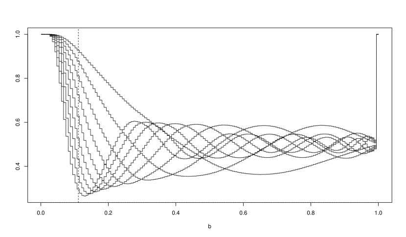
Figure 1: Numerical values of $P_{0,I_{n}}(\hat{\omega}_{\mathcal{W}}\geq 0)$ for $\mathcal{W}_{ij}=\mathbf{1}_{(-1,1)}((i-j)/(bn))$ as a function of $b$. Sample size $n=150$ and Assumption 3 holds with $k_{F}=k$ and for different values of $k\in\{2,3,4,\ldots,10\}$. The probabilities for $k=2$ correspond to the function with the largest value at the dashed vertical line, the probabilities for $k=3$ correspond to the function with the second largest value at the dashed vertical line, etc.

The assumption of $\mathcal{W}$ being data-independent, i.e., constant as a function of $y\in\mathbb{R}^{n}$, in the previous two corollaries is not satisfied for the important class of long-run-variance estimators that incorporate prewhitening or data-dependent bandwidth parameters (e.g., Andrews (1991), Andrews and Monahan (1992), and Newey and West (1994)). An additional complication for such estimators is that the corresponding weights matrix $\mathcal{W}(y)$, and thus also $\check{\Omega}_{\mathcal{W}}$, are in general not well-defined for every $y\in\mathbb{R}^{n}$. Nevertheless, after a careful structural analysis of such estimators (similar to the results obtained in Section 3.3 of Preinerstorfer (2017)), one can typically show that the resulting test statistic satisfies the assumptions of Theorem 5.2 above and thus one can obtain suitable versions of the above corollaries tailored towards test statistics based on specific classes of prewhitened long-run-variance estimators with data-dependent bandwidth parameters. To make this more compelling, we provide in the following such a result for a widely used procedure in that class. We consider a version of the AR(1)-prewhitened long-run-variance estimator based on auxiliary AR(1) models for bandwidth selection and the Quadratic-Spectral kernel as discussed in Andrews and Monahan (1992). This is a long-run-variance estimator as in (17), where the weights matrix is obtained as follows (the set where all involved quantities are well-defined is given in (21) further below): Let

$$\hat{\rho}(y)=\frac{\sum_{i=2}^{n}\hat{u}_{i}(y)\hat{u}_{i-1}(y)}{\sum_{i=1}^{n-1}\hat{u}_{i}^{2}(y)},$$ (20)

and define $\hat{v}_{i}(y)=\hat{u}_{i+1}(y)-\hat{\rho}(y)\hat{u}_{i}(y)$ for $i=1,\ldots,n-1$, which one can write in an obvious way as $\hat{v}(y)=\mathsf{A}(\hat{\rho}(y))\hat{u}(y)$ with $\rho\mapsto\mathsf{A}(\rho)\in\mathbb{R}^{(n-1)\times n}$ a continuous function on $\mathbb{R}$. Define the data-dependent bandwidth parameter $M_{\mathrm{AM}}$ via

$$M_{\mathrm{AM}}(y)=1.3221\left(n\frac{4\tilde{\rho}^{2}(y)}{(1-\tilde{\rho}(y))^{4}}\right)^{1/5}\quad\text{ with }\quad\tilde{\rho}(y)=\frac{\sum_{i=2}^{n-1}\hat{v}_{i}(y)\hat{v}_{i-1}(y)}{\sum_{i=1}^{n-2}\hat{v}_{i}^{2}(y)}.$$

The long-run-variance estimator $\hat{\omega}_{\mathcal{W}_{\mathrm{AM}}}$ is now obtained (granted the involved expressions are well-defined) by choosing $\mathcal{W}$ in (17) equal to

$$\mathcal{W}_{\mathrm{AM}}(y)=(1-\hat{\rho}(y))^{-2}\mathsf{A}^{\prime}(\hat{\rho}(y))\left[\kappa_{\mathrm{QS}}(|i-j|/M_{\mathrm{AM}}(y))\right]_{i,j=1}^{n-1}\mathsf{A}(\hat{\rho}(y)),$$

where $[\kappa_{\mathrm{QS}}(|i-j|/M_{\mathrm{AM}}(y))]_{i,j=1}^{n-1}$ is defined as $I_{n-1}$ in case $M_{\mathrm{AM}}(y)=0$ holds (cf., e.g., p. 821 in Andrews (1991) for a definition of the Quadratic-Spectral kernel $\kappa_{\mathrm{QS}}$). The corresponding covariance matrix estimator $\check{\Omega}_{\mathcal{W}_{\mathrm{AM}}}$ is then given by plugging $\hat{\omega}_{\mathcal{W}_{\mathrm{AM}}}$ into (16). The set where $\mathcal{W}_{\mathrm{AM}}$ (and hence $\check{\Omega}_{\mathcal{W}_{\mathrm{AM}}}$) is well-defined is easily seen to coincide with the set of all $y\in\mathbb{R}^{n}$ such that $\hat{\rho}(y)$ and $\tilde{\rho}(y)$ are both well-defined and are not equal to $1$, i.e., with the set

$$\left\{y\in\mathbb{R}^{n}:\sum_{i=1}^{n-1}\hat{u}_{i}(y)(\hat{u}_{i+1}(y)-\hat{u}_{i}(y))\neq 0,~{}\sum_{i=1}^{n-2}\hat{v}_{i}(y)(\hat{v}_{i+1}(y)-\hat{v}_{i}(y))\neq 0\right\}.$$ (21)

Define $N_{\mathrm{AM}}$ as the complement of the set (21) in $\mathbb{R}^{n}$. A result concerning size properties of polynomial trend tests based on the long-run-variance estimator $\hat{\omega}_{\mathcal{W}_{\mathrm{AM}}}$ is now obtained by combining Theorem 5.2 above with results obtained in Lemma D.3 in Appendix D, showing, in particular, that $\hat{\beta}$ and $\check{\Omega}_{\mathcal{W}_{\mathrm{AM}}}$ satisfy Assumptions 1 with $N=N_{\mathrm{AM}}$, provided $N_{\mathrm{AM}}\neq\mathbb{R}^{n}$ holds. Note that (i) the condition $N_{\mathrm{AM}}\neq\mathbb{R}^{n}$ only depends on properties of the design matrix $X$ and hence can be checked, and that (ii) in case $N_{\mathrm{AM}}=\mathbb{R}^{n}$, the matrix $\check{\Omega}_{\mathcal{W}_{\mathrm{AM}}}$ is nowhere well-defined, and tests based on this estimator hence break down in a trivial way.

Corollary 5.6.

Let $\mathfrak{F}\subseteq\mathfrak{F}_{\mathrm{all}}$ satisfy $\mathfrak{F}\supseteq\mathfrak{F}_{\mathrm{AR(}2\mathrm{)}}^{ext}$ and suppose Assumption 3 holds. Suppose further that $N_{\mathrm{AM}}\neq\mathbb{R}^{n}$. Then $\check{\beta}=\hat{\beta}$ and $\check{\Omega}=\check{\Omega}_{\mathcal{W}_{\mathrm{AM}}}$ satisfy Assumption 1 with $N=N_{\mathrm{AM}}$. Let $T$ be of the form (4) with $\check{\beta}=\hat{\beta}$, $\check{\Omega}=\check{\Omega}_{\mathcal{W}_{\mathrm{AM}}}$, and $N=N_{\mathrm{AM}}$. Then

$$\sup_{f\in\mathfrak{F}}P_{\mu_{0},\sigma^{2}\Sigma(f)}(T\geq C)=1$$

holds for every critical value $C$, $-\infty<C<\infty$, for every $\mu_{0}\in\mathfrak{M}_{0}$, and for every $\sigma^{2}\in(0,\infty)$.

Remark 5.7.

In the special case where Assumption 3 is satisfied with $R_{\cdot 1}\neq 0$, appropriate versions of Corollaries 5.4, 5.5, and 5.6 maintaining only $\mathfrak{F}\supseteq\mathfrak{F}_{\mathrm{AR(}1\mathrm{)}}$ can be obtained by perusing Remark 5.3. We abstain from spelling out details. A similar remark applies to Corollaries 5.8, 5.9, and 5.10 given in the next subsection.

5.1.2 Properties of some recently suggested tests for hypotheses on polynomial trends

In this subsection we discuss finite sample properties of classes of tests for polynomial trends that have been suggested in Vogelsang (1998) and Bunzel and Vogelsang (2005). We start with a discussion of the tests introduced in the former article. Vogelsang (1998) introduces two classes of tests for testing hypotheses on trends, in particular polynomial trends. From Section 3.2 of Vogelsang (1998) it is not difficult to see that these classes of test statistics (i.e., the classes referred to as $PS_{T}^{i}$ and $PSW_{T}^{i}$ in that reference) are (possibly up to a constant positive multiplicative factor that can be absorbed into the critical value) of the form (4). More specifically, the test statistics in Vogelsang (1998) are based on a combination of one of the two estimators

$$\check{\beta}_{V}(y)=\hat{\beta}_{VX}(Vy)=(X^{\prime}V^{\prime}VX)^{-1}X^{\prime}V^{\prime}Vy\quad\text{ for }V\in\{A,I_{n}\},$$ (22)

with a corresponding covariance estimator of the form

$$\check{\Omega}_{c,U,i,V}^{\mathrm{Vo}}(y)=n^{j(V)}s_{A,X}^{2}(y)\exp(cJ_{n,U}^{i}(y))R(X^{\prime}V^{\prime}VX)^{-1}R^{\prime},$$ (23)

for $i\in\{1,2\}$ and where $j(V)=1$ if $V=A$ and $j(V)=-1$ if $V=I_{n}$. Here $A$ is the $n\times n$-dimensional matrix that has $0$ above the main diagonal and $1$ on and below the main diagonal, $c\mathbb{\ }$is a real number, $U$ is an $n\times m$-dimensional matrix (with $m\geq 1$) such that $(X,U)$ is of full column-rank $k+m<n$. [In Vogelsang (1998) the column vectors of $U$ correspond to polynomial trends of an order exceeding the polynomial trends already contained in $\mathop{\mathrm{s}pan}(X)$.] Furthermore,

$$J_{n,U}^{1}(y)=n^{-1}\hat{\beta}_{(X,U)}^{\prime}(y)G^{\prime}\left(s_{I_{n},(X,U)}^{2}(y)G((X,U)^{\prime}(X,U))^{-1}G^{\prime}\right)^{-1}G\hat{\beta}_{(X,U)}(y),$$ (24)

and

$$J_{n,U}^{2}(y)=n^{-1}\hat{\beta}_{A(X,U)}^{\prime}(Ay)G^{\prime}\left(s_{A,(X,U)}^{2}(y)G((X,U)^{\prime}A^{\prime}A(X,U))^{-1}G^{\prime}\right)^{-1}G\hat{\beta}_{A(X,U)}(Ay),$$

with $G=(0,I_{m})\in\mathbb{R}^{m\times(k+m)}$, where we use the notation

$$s_{D_{1},D_{2}}^{2}(y)=n^{-1}y^{\prime}D_{1}^{\prime}\Pi_{\mathop{\mathrm{s}pan}(D_{1}D_{2})^{\bot}}D_{1}y$$

for nonsingular $D_{1}\in\mathbb{R}^{n\times n}$ and for $D_{2}\in\mathbb{R}^{n\times l}$ of rank $l\leq n$. It is obvious from the above expressions that the covariance estimator $\check{\Omega}_{c,U,i,V}^{\mathrm{Vo}}$ is not well-defined on all of $\mathbb{R}^{n}$. However, it is also not difficult to see that the set where such an estimator is well-defined coincides with $\mathbb{R}^{n}\backslash\mathop{\mathrm{s}pan}(X,U)$, see the proof of Lemma D.4 in Appendix D. We stress once more that the matrix $U$ used in the construction above is chosen in a particular way in Vogelsang (1998). We do not impose such a restriction here, because it would unnecessarily complicate the presentation of the result below, and because this restrictions is actually not necessary for establishing the result. The following result now shows, in particular, that the tests suggested in Vogelsang (1998) suffer from substantial size distortions in case $\mathfrak{F}\supseteq\mathfrak{F}_{AR(2)}^{ext}$.

Corollary 5.8.

Let $\mathfrak{F}\subseteq\mathfrak{F}_{\mathrm{all}}$ satisfy $\mathfrak{F}\supseteq\mathfrak{F}_{\mathrm{AR(}2\mathrm{)}}^{ext}$ and suppose Assumption 3 holds. Let $V\in\{A,I_{n}\}$, $c\in\mathbb{R}$, $i\in\{1,2\}$, and let $U$ be an $n\times m$-dimensional matrix with $m\geq 1$, $k+m<n$, such that $(X,U)$ is of full column-rank. Then $\check{\beta}=\check{\beta}_{V}$ and $\check{\Omega}=\check{\Omega}_{c,U,i,V}^{\mathrm{Vo}}$ satisfy Assumption 1 with $N=\mathop{\mathrm{s}pan}(X,U)$. Let $T$ be of the form (4) with $\check{\beta}=\check{\beta}_{V}$, $\check{\Omega}=\check{\Omega}_{c,U,i,V}^{\mathrm{Vo}}$, and $N=\mathop{\mathrm{s}pan}(X,U)$. Then

$$\sup_{f\in\mathfrak{F}}P_{\mu_{0},\sigma^{2}\Sigma(f)}(T\geq C)=1$$

holds for every critical value $C$, $-\infty<C<\infty$, for every $\mu_{0}\in\mathfrak{M}_{0}$, and for every $\sigma^{2}\in(0,\infty)$.

Next we turn to the tests introduced in Bunzel and Vogelsang (2005). We first discuss tests introduced in that article with data-independent tuning parameters and data-independent critical values: These tests are based on the OLS estimator $\hat{\beta}$ and two classes of covariance matrix estimators, both of which incorporate a tuning parameter $c\in\mathbb{R}$, and which are defined as

$$\check{\Omega}_{\mathcal{W},U,c}^{\mathrm{BV},J}(y)=\hat{\omega}_{\mathcal{W}}(y)\exp(cJ_{n,U}^{1}(y))R(X^{\prime}X)^{-1}R^{\prime},$$ (25)

where $U$ is an $n\times m$-dimensional matrix with $m\geq 1$ such that $(X,U)$ is of full column-rank $k+m<n$ (note that $\hat{\omega}_{\mathcal{W}}$ and $J_{n,U}^{1}$ have been defined in (17) and (24) above), and

$$\check{\Omega}_{\mathcal{W},c}^{\mathrm{BV}}(y)=\hat{\omega}_{\mathcal{W}}(y)\exp\left(cn^{-2}\frac{\hat{u}^{\prime}(y)A^{\prime}A\hat{u}(y)}{\hat{u}^{\prime}(y)\hat{u}(y)}\right)R(X^{\prime}X)^{-1}R^{\prime}$$ (26)

where $A$ has been defined below (23). The subsequent result applies, in particular, if $\mathcal{W}_{ij}=\kappa(|i-j|/M)$ where $M>0$ is a (fixed) real number and $\kappa$ is a kernel function such that $\mathcal{W}$ is positive definite, including the recommendation in Bunzel and Vogelsang (2005) to use the Daniell kernel. In that case, and more generally whenever $\Pi_{\mathop{\mathrm{s}pan}(X)^{\bot}}\mathcal{W}\Pi_{\mathop{\mathrm{s}pan}(X)^{\bot}}$ is nonzero and nonnegative definite (with $\mathcal{W}$ constant and symmetric), the subsequent corollary shows that the above mentioned tests in Bunzel and Vogelsang (2005) have size equal to one if $\mathfrak{F}\supseteq\mathfrak{F}_{AR(2)}^{ext}$; in case $\Pi_{\mathop{\mathrm{s}pan}(X)^{\bot}}\mathcal{W}\Pi_{\mathop{\mathrm{s}pan}(X)^{\bot}}$ is nonzero but not nonnegative definite, a lower bound on the size is obtained, which also provides an upper bound for the power in the case of i.i.d. errors. A discussion similar to the discussion following Corollary 5.5 also applies here (cf. also Figure 1).

Corollary 5.9.

Let $\mathfrak{F}\subseteq\mathfrak{F}_{\mathrm{all}}$ satisfy $\mathfrak{F}\supseteq\mathfrak{F}_{\mathrm{AR(}2\mathrm{)}}^{ext}$ and suppose Assumption 3 holds. Suppose that $\mathcal{W}$ is constant and symmetric, that $\Pi_{\mathop{\mathrm{s}pan}(X)^{\bot}}\mathcal{W}\Pi_{\mathop{\mathrm{s}pan}(X)^{\bot}}$ is nonzero, and that $c\in\mathbb{R}$. Furthermore, for the statements that involve $U$, suppose $U$ is an $n\times m$-dimensional matrix with $m\geq 1$ such that $(X,U)$ is of full column-rank $k+m<n$. Then, $\check{\beta}=\hat{\beta}$ and $\check{\Omega}=\check{\Omega}_{\mathcal{W},c}^{\mathrm{BV}}$ ($\check{\beta}=\hat{\beta}$ and $\check{\Omega}=\check{\Omega}_{\mathcal{W},U,c}^{\mathrm{BV},J}$, respectively) satisfy Assumption 1 with $N=\mathop{\mathrm{s}pan}(X)$ ($N=\mathop{\mathrm{s}pan}(X,U)$, respectively). Let $T$ be of the form (4) with $\check{\beta}=\hat{\beta}$, $\check{\Omega}=\check{\Omega}_{\mathcal{W},c}^{\mathrm{BV}}$, and $N=\mathop{\mathrm{s}pan}(X)$, or with $\check{\beta}=\hat{\beta}$, $\check{\Omega}=\check{\Omega}_{\mathcal{W},U,c}^{\mathrm{BV},J}$, and $N=\mathop{\mathrm{s}pan}(X,U)$. Then

$$P_{0,I_{n}}(\hat{\omega}_{\mathcal{W}}\geq 0)\leq\sup_{f\in\mathfrak{F}}P_{\mu_{0},\sigma^{2}\Sigma(f)}(T\geq C)$$

holds for every critical value $C$, $-\infty<C<\infty$, for every $\mu_{0}\in\mathfrak{M}_{0}$, and for every $\sigma^{2}\in(0,\infty)$. The lower bound equals $1$ in case $\Pi_{\mathop{\mathrm{s}pan}(X)^{\bot}}\mathcal{W}\Pi_{\mathop{\mathrm{s}pan}(X)^{\bot}}$ is nonnegative definite. Furthermore, for every $0\leq C<\infty$ the lower bound in the previous display is an upper bound for the maximal power of the test under i.i.d. errors, i.e.,

$$\sup_{\mu_{1}\in\mathfrak{M}_{1}}\sup_{0<\sigma^{2}<\infty}P_{\mu_{1},\sigma^{2}I_{n}}(T\geq C)\leq P_{0,I_{n}}(\hat{\omega}_{\mathcal{W}}\geq 0).$$ (27)

We shall now turn to the approach Bunzel and Vogelsang (2005) suggest for practical applications. This approach is based on a data-driven selection of the weights matrix $\mathcal{W}$ and of the tuning parameter $c$, and on a data-driven selection of the critical value $C$. Their approach is as follows: Bunzel and Vogelsang (2005) focus on $\hat{\omega}_{\mathcal{W}}$ based on the Daniell kernel. More specifically, they set $\mathcal{W}_{ij}=\kappa_{D}(|i-j|/\max(bn,2))$ (cf. Bunzel and Vogelsang (2005), Appendix B, for a definition of the Daniell kernel). Recall that, regardless of the value of $b$, the matrix with elements $\mathcal{W}_{ij}=\kappa_{D}(|i-j|/\max(bn,2))$ based on the Daniell kernel is positive definite. The authors recommend to choose $b$ as a positive piecewise constant function of $\hat{\rho}$ (which has been defined in (20) above), more precisely, for constants $a_{i}\in(0,\infty)$, $i=0,\ldots,m^{\prime}$ ($m^{\prime}\in\mathbb{N}$), and $\bar{a}_{i}\in\mathbb{R}$, $i=1,\ldots,m^{\prime}$, they suggest to use

$$b_{\mathrm{BV}}(y,a,\bar{a})=a_{0}+\sum_{i=1}^{{m^{\prime}}}a_{i}\mathbf{1}_{[\bar{a}_{i},\infty)}(\hat{\rho}(y)).$$

For a recommendation concerning the choice of these constants see Bunzel and Vogelsang (2005), p. 388. Furthermore, Bunzel and Vogelsang (2005) suggest to choose their data-driven critical value $C$ and a data-driven tuning parameter $c$ as a polynomial function of $b_{\mathrm{BV}}(y,a,\bar{a})$, respectively. More precisely, for constants $h_{0},\ldots,h_{m^{\prime\prime}}\in\mathbb{R}$ ($m^{\prime\prime}\in\mathbb{N}$, $h_{m^{\prime\prime}}\neq 0$) and $p_{0},\ldots,p_{m^{{}^{\prime\prime\prime}}}\in\mathbb{R}$ ($m^{\prime\prime\prime}\in\mathbb{N}$, $p_{m^{\prime\prime\prime}}\neq 0$) they suggest to use

$$C_{\mathrm{BV}}(y,h)=\sum_{i=0}^{m^{\prime\prime}}h_{i}(b_{\mathrm{BV}}(y,a,\bar{a}))^{i}\quad\text{ and }\quad c_{\mathrm{BV}}(y,p)=\sum_{i=0}^{m^{\prime\prime\prime}}p_{i}(b_{\mathrm{BV}}(y,a,\bar{a}))^{i}.$$

Then they set

$$\mathcal{W}_{\mathrm{BV}}(y)=\left[\kappa_{D}(|i-j|/\max(b_{\mathrm{BV}}(y,a,\bar{a})n,2))\right]_{i,j=1}^{n},$$

and define, in correspondence with (25) and (26), the covariance estimators

$$\check{\Omega}_{U,a,\bar{a},h,p}^{\mathrm{BV},J}(y)=\hat{\omega}_{\mathcal{W}_{\mathrm{BV}}}(y)\exp\left(c_{\mathrm{BV}}(y,p)J_{n,U}^{1}(y)\right)R(X^{\prime}X)^{-1}R^{\prime}$$

and

$$\check{\Omega}_{a,\bar{a},h,p}^{\mathrm{BV}}(y)=\hat{\omega}_{\mathcal{W}_{\mathrm{BV}}}(y)\exp\left(c_{\mathrm{BV}}(y,p)n^{-2}\frac{\hat{u}^{\prime}(y)A^{\prime}A\hat{u}(y)}{\hat{u}^{\prime}(y)\hat{u}(y)}\right)R(X^{\prime}X)^{-1}R^{\prime}.$$

The vectors of (constant) tuning parameters $a=(a_{0},\ldots,a_{m^{\prime}})^{\prime}$, $\bar{a}=(\bar{a}_{1},\ldots,\bar{a}_{m^{\prime}})^{\prime}$, $h=(h_{0},\ldots,h_{m^{\prime\prime}})^{\prime}$, and $p=(p_{0},\ldots,p_{m^{\prime\prime\prime}})^{\prime}$ this approach is based on are tabulated in Bunzel and Vogelsang (2005) for certain cases, and need to be obtained numerically, following the rationale in Bunzel and Vogelsang (2005), for the cases not tabulated in that paper. Furthermore, the data-driven tuning parameters $b_{\mathrm{BV}}$ and $c_{\mathrm{BV}}$ as well as the data-driven critical value $C_{\mathrm{BV}}$ are well-defined for a given $y\in\mathbb{R}^{n}$ if and only if $\hat{\rho}(y)$ is well-defined, i.e., these quantities are well-defined on the complement of the closed set

$$\tilde{N}:=\left\{y\in\mathbb{R}^{n}:\sum_{i=1}^{n-1}\hat{u}_{i}^{2}(y)=0\right\}.$$ (28)

Clearly, $\mathop{\mathrm{s}pan}(X)$ is contained in $\tilde{N}$. Hence, it is not difficult to see that the estimator $\check{\Omega}_{a,\bar{a},h,p}^{\mathrm{BV}}$ is well-defined on $\mathbb{R}^{n}\backslash\tilde{N}$ and that the estimator $\check{\Omega}_{U,a,\bar{a},h,p}^{\mathrm{BV},J}$ is well-defined on $\mathbb{R}^{n}\backslash(\mathop{\mathrm{s}pan}(X,U)\cup\tilde{N})$. In fact, under Assumption 3 we have that $\tilde{N}=\mathop{\mathrm{s}pan}(X)$ (see the proof of the subsequent corollary). Consequently, under Assumption 3, the estimator $\check{\Omega}_{a,\bar{a},h,p}^{\mathrm{BV}}$ is well defined on $\mathbb{R}^{n}\backslash\mathop{\mathrm{s}pan}(X)$ and $\check{\Omega}_{U,a,\bar{a},h,p}^{\mathrm{BV},J}$ is well-defined on $\mathbb{R}^{n}\backslash\mathop{\mathrm{s}pan}(X,U)$. [In order that the data-driven critical value is also defined for every $y$, we set $C_{\mathrm{BV}}(y,h)$ equal to an arbitrary value ($0$, say) on the null-set $\tilde{N}$. Of course, the choice of assignment on this null-set is inconsequential for the result below.]

The following corollary shows that the tests for hypotheses concerning polynomial trends based on data-driven tuning parameters and a data-driven critical value as suggested in Bunzel and Vogelsang (2005) have size one in case $\mathfrak{F}\supseteq\mathfrak{F}_{AR(2)}^{ext}$. The proof of this is based on a similar approach as used in the proof of Corollary 5.9 above, but has to deal with the fact that the choice of the tuning parameters and the critical value is data-driven, and hence is more involved. In particular, it turns out that in order for Assumption 1 to be satisfied for the covariance estimators used here, one has to work with null-sets $N_{\mathrm{BV},U}$ and $N_{\mathrm{BV}}$ that are larger than $\mathop{\mathrm{s}pan}(X,U)$ and $\mathop{\mathrm{s}pan}(X)$, respectively.

Corollary 5.10.

Let $\mathfrak{F}\subseteq\mathfrak{F}_{\mathrm{all}}$ satisfy $\mathfrak{F}\supseteq\mathfrak{F}_{\mathrm{AR(}2\mathrm{)}}^{ext}$ and suppose Assumption 3 holds. Let $a_{i}\in(0,\infty)$ for $i=0,\ldots,m^{\prime}$ ($m^{\prime}\in\mathbb{N}$), $\bar{a}_{i}\in\mathbb{R}$ for $i=1,\ldots,m^{\prime}$, $h_{i}\in\mathbb{R}$ for $i=0,\ldots,m^{\prime\prime}$ with $h_{m^{\prime\prime}}\neq 0$ and $m^{\prime\prime}\in\mathbb{N}$, and $p_{i}\in\mathbb{R}$ for $i=0,\ldots,m^{\prime\prime\prime}$ with $p_{m^{\prime\prime\prime}}\neq 0$ and $m^{\prime\prime\prime}\in\mathbb{N}$. Furthermore, for the statements that involve $U$, suppose $U$ is an $n\times m$-dimensional matrix with $m\geq 1$ such that $(X,U)$ is of full column-rank $k+m<n$. Then, $\check{\beta}=\hat{\beta}$ and $\check{\Omega}=\check{\Omega}_{a,\bar{a},h,p}^{\mathrm{BV}}$ satisfy Assumption 1 with $N=N_{\mathrm{BV}}$ (defined in Lemma D.6 in Appendix D), and $\check{\beta}=\hat{\beta}$ and $\check{\Omega}=\check{\Omega}_{U,a,\bar{a},h,p}^{\mathrm{BV},J}$ satisfy Assumption 1 with $N=N_{\mathrm{BV},U}$ (defined in Lemma D.6). Let $T$ be of the form (4) with $\check{\beta}=\hat{\beta}$, $\check{\Omega}=\check{\Omega}_{a,\bar{a},h,p}^{\mathrm{BV}}$, and $N=N_{\mathrm{BV}}$, or with $\check{\beta}=\hat{\beta}$, $\check{\Omega}=\check{\Omega}_{U,a,\bar{a},h,p}^{\mathrm{BV},J}$, and $N=N_{\mathrm{BV},U}$. Then

$$\sup_{f\in\mathfrak{F}}P_{\mu_{0},\sigma^{2}\Sigma(f)}(\{y\in\mathbb{R}^{n}:T(y)\geq C_{\mathrm{BV}}(y,h)\})=1$$

holds for every $\mu_{0}\in\mathfrak{M}_{0}$ and for every $\sigma^{2}\in(0,\infty)$.

Remark 5.11.

Alternatively one can consider $T^{\ast}$, where

$$T^{\ast}(y)=(R\hat{\beta}(y)-r)^{\prime}\left(\check{\Omega}_{a,\bar{a},h,p}^{\mathrm{BV}}(y)\right)^{-1}(R\hat{\beta}(y)-r)$$

for all $y\in\mathbb{R}^{n}\backslash\mathop{\mathrm{s}pan}(X)$ such that $\check{\Omega}_{a,\bar{a},h,p}^{\mathrm{BV}}(y)$ is nonsingular, and where $T^{\ast}(y)=0$ else, (and we can similarly define a test statistic $T^{\ast\ast}$ with $\check{\Omega}_{U,a,\bar{a},h,p}^{\mathrm{BV},J}$ and $\mathop{\mathrm{s}pan}(X,U)$ in place of $\check{\Omega}_{a,\bar{a},h,p}^{\mathrm{BV}}$ and $\mathop{\mathrm{s}pan}(X)$, respectively). While $T^{\ast}$ and $T^{\ast\ast}$ are well-defined test statistics, we are not guaranteed that $\hat{\beta}$ and $\check{\Omega}_{a,\bar{a},h,p}^{\mathrm{BV}}$ ($\hat{\beta}$ and $\check{\Omega}_{U,a,\bar{a},h,p}^{\mathrm{BV},J}$, respectively) satisfy Assumption 1 with $N=\mathop{\mathrm{s}pan}(X)$ ($N=\mathop{\mathrm{s}pan}(X,U)$, respectively). However, $T^{\ast}$ as well as $T^{\ast\ast}$ differ from the corresponding test statistics considered in the preceding corollary at most on a null-set, hence the conclusions of the corollary carry over to $T^{\ast}$ and $T^{\ast\ast}$.

5.2 Cyclical trends

We here consider briefly the case when one tests hypotheses concerning a cyclical trend, i.e., when the following assumption is satisfied:

Assumption 4.

Suppose that $X=(E_{n,0}(\omega),\tilde{X})$ for some $\omega\in(0,\pi)$ where $\tilde{X}$ is an $n\times(k-2)$-dimensional matrix such that $X$ has rank $k$ (here $\tilde{X}$ is the empty matrix if $k=2$). Furthermore, suppose that the restriction matrix $R$ has a nonzero column $R_{\cdot i}$ for some $i=1,2$, i.e., the hypothesis involves coefficients of the cyclical component.

Under this assumption we obtain the subsequent theorem from Theorem 3.10.

Theorem 5.12.

Let $\mathfrak{F}\subseteq\mathfrak{F}_{\mathrm{all}}$ satisfy $\mathfrak{F}\supseteq\mathfrak{F}_{\mathrm{AR(}2\mathrm{)}}$ and suppose Assumption 4 holds. Let $T$ be a nonsphericity-corrected F-type test statistic of the form (4) based on $\check{\beta}$ and $\check{\Omega}$ satisfying Assumption 1 with $N=\emptyset$. Furthermore, assume that $\check{\Omega}(y)$ is nonnegative definite for every $y\in\mathbb{R}^{n}$. Then

$$\sup_{f\in\mathfrak{F}}P_{\mu_{0},\sigma^{2}\Sigma(f)}(T\geq C)=1$$

holds for every critical value $C$, $-\infty<C<\infty$, for every $\mu_{0}\in\mathfrak{M}_{0}$, and for every $\sigma^{2}\in(0,\infty)$.

Under a slightly stronger condition on $\mathfrak{F}$, the following theorem is applicable in case the assumption that $N=\emptyset$ or the nonnegative definiteness assumption on $\check{\Omega}$ in the previous theorem are violated.

Theorem 5.13.

Let $\mathfrak{F}\subseteq\mathfrak{F}_{\mathrm{all}}$ satisfy $\mathfrak{F}\supseteq\mathfrak{F}_{\mathrm{AR(}2\mathrm{)}}^{ext}$. Suppose Assumption 4 holds. Let $T$ be a nonsphericity-corrected F-type test statistic of the form (4) based on $\check{\beta}$ and $\check{\Omega}$ satisfying Assumption 1. Furthermore, assume that $\check{\Omega}$ also satisfies Assumption 2. Then for every critical value $C$, $-\infty<C<\infty$, for every $\mu_{0}\in\mathfrak{M}_{0}$, and for every $\sigma^{2}\in(0,\infty)$ it holds that

$$P_{0,I_{n}}(\check{\Omega}\text{ is nonnegative definite})\leq K(\omega)\leq\sup_{f\in\mathfrak{F}}P_{\mu_{0},\sigma^{2}\Sigma(f)}\left(T\geq C\right),$$

where $K(\omega)$ is defined in Theorem 3.12.

Using these results, one can now obtain similar results as in Subsection 5.1.2 concerning the tests developed in Vogelsang (1998) and Bunzel and Vogelsang (2005) under Assumption 4. Due to space constraints, however, we do not spell out the details.

Remark 5.14.

(The cases $\omega=0$ or $\omega=\pi$) (i) In case $\omega=0$ (or $\omega=\pi$) consider Assumption 4 with the understanding that $X=(\bar{E}_{n,0}(\omega),\tilde{X})$, that $\tilde{X}$ is now $n\times(k-1)$-dimensional, and that $R_{\cdot 1}\neq 0$, where $\bar{E}_{n,0}(\omega)$ denotes the first column of $E_{n,0}(\omega)$. Then Theorems 5.12 and 5.13 continue to hold with this interpretation of Assumption 4. Also note that the case $\omega=0$ can be subsumed under the results of Subsection 5.1 by setting $k_{F}=1$.

(ii) In case $\omega=0$ (or $\omega=\pi$), Theorem 5.12 (with the before mentioned interpretation of Assumption 4) in fact continues to hold under the weaker assumption that $\mathfrak{F}\supseteq\mathfrak{F}_{\mathrm{AR(}1\mathrm{)}}$. This follows from Part 3 of Corollary 5.17 in Preinerstorfer and Pötscher (2016) upon noting that $\mathcal{Z}=\mathop{\mathrm{s}pan}(\bar{E}_{n,0}(\omega))$ is a concentration space of the covariance model $\mathfrak{C}(\mathfrak{F})$, that $\check{\Omega}$ vanishes on $\mathop{\mathrm{s}pan}(X)\supseteq\mathcal{Z}$ as a consequence of the assumption $N=\emptyset$ (see the discussion following (27) in Preinerstorfer and Pötscher (2016)), and that $R\check{\beta}(z)\neq 0$ for every $z\in\mathcal{Z}$ with $z\neq 0$.

(iii) In case $\omega=0$ (or $\omega=\pi$), Theorem 5.13 (with the before mentioned interpretation of Assumption 4) also continues to hold under the weaker assumption that $\mathfrak{F}\supseteq\mathfrak{F}_{\mathrm{AR(}1\mathrm{)}}$ if $\bar{\xi}_{\omega}(x)$ in the definition of $K(\omega)$ is now replaced by $\breve{\xi}_{\omega}(x)$ defined as

$$\breve{\xi}_{\omega}(x) = (R\hat{\beta}_{X}(\bar{E}_{n,0}(\omega)x))^{\prime}\check{\Omega}^{-1}\left(\left(\left(\bar{E}_{n,0}(\omega)\bar{E}_{n,0}(\omega)^{\prime}\right)^{1/2}+D(\omega)^{1/2}\right)\mathbf{G}\right)R\hat{\beta}_{X}(\bar{E}_{n,0}(\omega)x)$$

$$= x^{2}R_{\cdot 1}^{\prime}\check{\Omega}^{-1}\left(\left(\left(\bar{E}_{n,0}(\omega)\bar{E}_{n,0}(\omega)^{\prime}\right)^{1/2}+D(\omega)^{1/2}\right)\mathbf{G}\right)R_{\cdot 1}$$

on the event where $\{((\bar{E}_{n,0}(\omega)\bar{E}_{n,0}(\omega)^{\prime})^{1/2}+D(\omega)^{1/2})\mathbf{G}\in\mathbb{R}^{n}\backslash N^{\ast}\}$ and by $\breve{\xi}_{\omega}(x)=0$ otherwise, and if the distribution $P_{0,I_{n}}$ appearing in the lower bound is replaced by $P_{0,\Phi(\omega)}$ where $\Phi(\omega)=\bar{E}_{n,0}(\omega)\bar{E}_{n,0}(\omega)^{\prime}+D(\omega)$ is nonsingular. Note that then $K(\omega)$ reduces to $P_{0,\Phi(\omega)}(R_{\cdot 1}^{\prime}\check{\Omega}^{-1}R_{\cdot 1}\geq 0)$. Here $D(0)$ is the matrix $D$ given in Part 3 and $D(\pi)$ is the matrix $D$ given in Part 4 of Lemma G.1 in Preinerstorfer and Pötscher (2016). This can be proved by making use of Theorem 5.19 and Lemma G.1 in Preinerstorfer and Pötscher (2016).

Appendix A Appendix: Proofs and auxiliary results for Section 3.1

Lemma A.1.

Let $\mathfrak{C}$ be a covariance model and let $\mathcal{L}$ be a linear subspace of $\mathbb{R}^{n}$ with $\dim(\mathcal{L})=l<n$. Let $\mathfrak{C}^{\sharp}=\left\{\Sigma^{\sharp}:\Sigma\in\mathfrak{C}\right\}$ and $\mathfrak{C}^{\natural}=\left\{\Sigma^{\natural}:\Sigma\in\mathfrak{C}\right\}$, where $\Sigma^{\sharp}=\mathcal{L}(\Sigma)+\lambda_{l+1}(\mathcal{L}(\Sigma))\Pi_{\mathcal{L}}$ and where $\Sigma^{\natural}=\mathcal{L}(\Sigma)+\Pi_{\mathcal{L}}$; here $\lambda_{l+1}(\mathcal{L}(\Sigma))$ denotes the $(l+1)$-th eigenvalue of $\mathcal{L}(\Sigma)$ counting (with multiplicity) from smallest to largest. Then $\mathfrak{C}^{\sharp}$ and $\mathfrak{C}^{\natural}$ are covariance models. Furthermore, the collection of concentration spaces of $\mathfrak{C}^{\sharp}$ coincides with $\mathbb{J}(\mathcal{L},\mathfrak{C})$, and the collection of concentration spaces of $\mathfrak{C}^{\natural}$ coincides with the collection $\left\{\mathcal{S}+\mathcal{L}:\mathcal{S}\in\mathbb{J}(\mathcal{L},\mathfrak{C})\right\}$.

Proof: 1. That $\mathfrak{C}^{\sharp}$ and $\mathfrak{C}^{\natural}$ are covariance models is obvious since the elements of these two collections are clearly symmetric and positive definite matrices (as $\lambda_{l+1}(\mathcal{L}(\Sigma))>0$ by construction).

2. Suppose $\mathcal{S}\in\mathbb{J}(\mathcal{L},\mathfrak{C})$. Then $\mathcal{S}=\mathop{\mathrm{s}pan}(\bar{\Sigma})$ for some $\bar{\Sigma}\in\mathop{\mathrm{c}l}(\mathcal{L}(\mathfrak{C}))$ with $\mathop{\mathrm{r}ank}(\bar{\Sigma})<n-l$. In particular, $\bar{\Sigma}$ is the limit of $\mathcal{L}(\Sigma_{m})$ for a sequence $\Sigma_{m}\in\mathfrak{C}$. But then $\Sigma_{m}^{\sharp}=\mathcal{L}(\Sigma_{m})+\lambda_{l+1}(\mathcal{L}(\Sigma_{m}))\Pi_{\mathcal{L}}$ belongs to $\mathfrak{C}^{\sharp}$ and converges to $\bar{\Sigma}$ for $m\rightarrow\infty$, since $\lambda_{l+1}(\mathcal{L}(\Sigma_{m}))$ converges to $\lambda_{l+1}(\bar{\Sigma})$, which equals zero as a consequence of $\mathop{\mathrm{r}ank}(\bar{\Sigma})<n-l$. This shows that $\mathop{\mathrm{s}pan}(\bar{\Sigma})$, and hence $\mathcal{S}$, is a concentration space of $\mathfrak{C}^{\sharp}$. Conversely, suppose $\mathcal{Z}$ is a concentration space of $\mathfrak{C}^{\sharp}$. Then $\mathcal{Z}=\mathop{\mathrm{s}pan}(\breve{\Sigma})$ for some singular matrix that is the limit of some sequence $\Sigma_{m}^{\sharp}\in\mathfrak{C}^{\sharp}$. In particular, $\Sigma_{m}^{\sharp}=\mathcal{L}(\Sigma_{m})+\lambda_{l+1}(\mathcal{L}(\Sigma_{m}))\Pi_{\mathcal{L}}$ holds for some sequence $\Sigma_{m}\in\mathfrak{C}$. Since the matrices $\mathcal{L}(\Sigma_{m})$ reside in the unit sphere in $\mathbb{R}^{n\times n}$, we have convergence of $\mathcal{L}(\Sigma_{m_{i}})$ to a limit $\bar{\Sigma}\in\mathbb{R}^{n\times n}$ along an appropriate subsequence $m_{i}$; in particular, $\bar{\Sigma}\in\mathop{\mathrm{c}l}(\mathcal{L}(\mathfrak{C}))$ follows. Furthermore, we conclude that $\Sigma_{m_{i}}^{\sharp}$ converges to $\bar{\Sigma}+\lambda_{l+1}(\bar{\Sigma})\Pi_{\mathcal{L}}$, and hence obtain the equality $\breve{\Sigma}=\bar{\Sigma}+\lambda_{l+1}(\bar{\Sigma})\Pi_{\mathcal{L}}$. Since $\bar{\Sigma}$ is certainly symmetric and nonnegative definite, we have that $\lambda_{l+1}(\bar{\Sigma})\geq 0$. Note that $\bar{\Sigma}x=0$ for every $x\in\mathcal{L}$ by construction of $\bar{\Sigma}$. Hence $\mathop{\mathrm{r}ank}(\bar{\Sigma})\leq n-l$ must hold. If $\mathop{\mathrm{r}ank}(\bar{\Sigma})=n-l$ would hold we would have $\lambda_{l+1}(\bar{\Sigma})>0$, implying that $\bar{\Sigma}+\lambda_{l+1}(\bar{\Sigma})\Pi_{\mathcal{L}}$ is nonsingular, contradicting singularity of $\breve{\Sigma}$. Consequently, $\mathop{\mathrm{r}ank}(\bar{\Sigma})<n-l$ and $\lambda_{l+1}(\bar{\Sigma})=0$ must hold, implying that $\mathcal{S}=\mathop{\mathrm{s}pan}(\bar{\Sigma})$ belongs to $\mathbb{J}(\mathcal{L},\mathfrak{C})$ and that $\breve{\Sigma}=\bar{\Sigma}$ holds. But this shows $\mathcal{Z}=\mathcal{S}\in\mathbb{J}(\mathcal{L},\mathfrak{C})$.

3. Suppose $\mathcal{S}\in\mathbb{J}(\mathcal{L},\mathfrak{C})$. Then $\mathcal{S}=\mathop{\mathrm{s}pan}(\bar{\Sigma})$ for some $\bar{\Sigma}\in\mathop{\mathrm{c}l}(\mathcal{L}(\mathfrak{C}))$ with $\mathop{\mathrm{r}ank}(\bar{\Sigma})<n-l$. In particular, $\bar{\Sigma}$ is the limit of $\mathcal{L}(\Sigma_{m})$ for a sequence $\Sigma_{m}\in\mathfrak{C}$. But then $\Sigma_{m}^{\natural}=\mathcal{L}(\Sigma_{m})+\Pi_{\mathcal{L}}$ belongs to $\mathfrak{C}^{\natural}$ and converges to $\bar{\Sigma}+\Pi_{\mathcal{L}}$ for $m\rightarrow\infty$. Now $\bar{\Sigma}+\Pi_{\mathcal{L}}$ is singular since $\mathop{\mathrm{r}ank}(\bar{\Sigma})<n-l$. Hence, $\mathop{\mathrm{s}pan}(\bar{\Sigma}+\Pi_{\mathcal{L}})$ is a concentration space of $\mathfrak{C}^{\natural}$ and $\mathop{\mathrm{s}pan}(\bar{\Sigma}+\Pi_{\mathcal{L}})=\mathop{\mathrm{s}pan}(\bar{\Sigma})+\mathcal{L}=\mathcal{S}+\mathcal{L}$ clearly holds. This proves one direction. Conversely, suppose $\mathcal{Z}$ is a concentration space of $\mathfrak{C}^{\natural}$. Then $\mathcal{Z}=\mathop{\mathrm{s}pan}(\breve{\Sigma})$ for some singular matrix that is the limit of some sequence $\Sigma_{m}^{\natural}\in\mathfrak{C}^{\natural}$, where $\Sigma_{m}^{\natural}=\mathcal{L}(\Sigma_{m})+\Pi_{\mathcal{L}}$ for some $\Sigma_{m}\in\mathfrak{C}$. By the same compactness argument as before, we have $\mathcal{L}(\Sigma_{m_{i}})\rightarrow\bar{\Sigma}$ implying that $\bar{\Sigma}\in\mathop{\mathrm{c}l}(\mathcal{L}(\mathfrak{C}))$. Furthermore, we immediately arrive at $\breve{\Sigma}=\bar{\Sigma}+\Pi_{\mathcal{L}}$. As before it follows that $\mathop{\mathrm{r}ank}(\bar{\Sigma})<n-l$ must hold and hence that $\mathcal{S}=\mathop{\mathrm{s}pan}(\bar{\Sigma})\in\mathbb{J}(\mathcal{L},\mathfrak{C})$. But then $\mathcal{Z}=\mathop{\mathrm{s}pan}(\breve{\Sigma})=\mathop{\mathrm{s}pan}(\bar{\Sigma}+\Pi_{\mathcal{L}})=\mathop{\mathrm{s}pan}(\bar{\Sigma})+\mathcal{L}$ holds, implying the result. $\blacksquare$

Remark A.2.

(i) By construction $\mathbb{J}(\mathcal{L},\mathfrak{C})=\mathbb{J}(\mathcal{L},\mathfrak{C}^{\sharp})=\mathbb{J}(\mathcal{L},\mathfrak{C}^{\natural})$. Furthermore, all three collections coincide with the collection of all concentration spaces of $\mathfrak{C}^{\sharp}$ (the union over which is $J(\mathfrak{C}^{\sharp})$ in the notation of Preinerstorfer and Pötscher (2016)).

(ii) The sum $\mathcal{S}+\mathcal{L}$ is an orthogonal sum and hence $\mathcal{S}$ is uniquely determined.

(iii) The map $\Sigma\mapsto\Sigma^{\sharp}$ is surjective from $\mathfrak{C}$ to $\mathfrak{C}^{\sharp}$ by definition, and the analogous statement holds for the map $\Sigma\mapsto\Sigma^{\natural}$. But these maps need not be injective.

Lemma A.3.

Let $\mathfrak{C}$ be a covariance model and let $\mathcal{L}$ be a linear subspace of $\mathbb{R}^{n}$ with $\dim(\mathcal{L})<n$. Furthermore, let $W\subseteq\mathbb{R}^{n}$ be a rejection region of a test, which is $G(a+\mathcal{L})$-invariant for some $a\in\mathbb{R}^{n}$. Then for every $\sigma$, $0<\sigma<\infty$, and every $\Sigma\in\mathfrak{C}$ we have

$$P_{a,\sigma^{2}\Sigma}(W)=P_{a,\sigma^{2}\mathcal{L}(\Sigma)}(W)=P_{a,\sigma^{2}\Sigma^{\sharp}}(W)=P_{a,\sigma^{2}\Sigma^{\natural}}(W).$$

Furthermore, these probabilities do not depend on $\sigma$ and they are unaffected if $a$ is replaced by an arbitrary element of $a+\mathcal{L}$.

Proof: The first claim is essentially proved by the argument establishing (B.1) in Appendix B of Pötscher and Preinerstorfer (2018). The second claim is an immediate consequence of the assumed invariance (cf. also Proposition 5.4 in Preinerstorfer and Pötscher (2016)). $\blacksquare$

Proof of Theorem 3.1: By monotonicity w.r.t. $C$ we may assume $C>0$. Note that $\dim(\mathfrak{M}_{0}^{lin})=k-q<n$ by our general model assumptions. Since $T$ is $G(\mathfrak{M}_{0})$-invariant by Lemma 5.16 in Preinerstorfer and Pötscher (2016), the preceding Lemma A.3, applied with $\mathcal{L}=\mathfrak{M}_{0}^{lin}$ and $a=\mu_{0}$, hence shows that it suffices to prove the theorem with $\mathfrak{C}$ replaced by $\mathfrak{C}^{\sharp}$. By Lemma A.1, also applied with $\mathcal{L}=\mathfrak{M}_{0}^{lin}$, the space $\mathcal{S}$ appearing in the formulation of the theorem is a concentration space of $\mathfrak{C}^{\sharp}$. We now apply Part 3 of Corollary 5.17 of Preinerstorfer and Pötscher (2016) to the linear model (1) considered in the present paper, but with $\mathfrak{C}$ replaced by $\mathfrak{C}^{\sharp}$. All assumptions of that result, except for the assumption that $\check{\Omega}(z)=0$ and $R\check{\beta}(z)\neq 0$ simultaneously hold $\lambda_{\mathcal{S}}$-almost everywhere, are easily seen to be satisfied. We verify the remaining assumption now as follows: The discussion following (27) in Section 5.4 of Preinerstorfer and Pötscher (2016) shows that in case $N=\emptyset$ (which is assumed here) $\check{\Omega}(z)=0$ holds for every $z\in\mathrm{\mathop{\mathrm{s}pan}}(X)$, and thus for every $z\in\mathcal{S}$ (since $\mathcal{S}\subseteq\mathrm{\mathop{\mathrm{s}pan}}(X)$ has been assumed). Hence, $\check{\Omega}(z)=0$ $\lambda_{\mathcal{S}}$-almost everywhere follows (note that $\lambda_{\mathcal{S}}(\mathbb{R}^{n}\backslash\mathcal{S})=0$ trivially holds). Furthermore, Assumption 1 together with $N=\emptyset$ imply that $\check{\beta}(X\gamma)=\check{\beta}(\varepsilon\cdot 0+X\gamma)=\varepsilon\check{\beta}(0)+\gamma$ for every $\gamma\in\mathbb{R}^{k}$ and every $\varepsilon\neq 0$, which of course implies $\check{\beta}(X\gamma)=\gamma$ for every $\gamma\in\mathbb{R}^{k}$. Since we have assumed $\mathcal{S}\subseteq\mathrm{\mathop{\mathrm{s}pan}}(X)$, it follows on the one hand that for every $z\in\mathcal{S}$ we have $R\check{\beta}(z)=0$ if and only if $z\in\mathfrak{M}_{0}^{lin}$. On the other hand, by construction $\mathcal{S}\subseteq(\mathfrak{M}_{0}^{lin})^{\bot}$ holds, showing that $R\check{\beta}(z)\neq 0$ must hold for all nonzero $z\in\mathcal{S}$ in view of the fact that $\mathcal{S}\subseteq\mathrm{\mathop{\mathrm{s}pan}}(X)$ has been assumed. Since $\mathcal{S}$ can not be zero-dimensional in view of its definition (cf. the discussion in Pötscher and Preinerstorfer (2018) following Definition 5.1), $\lambda_{\mathcal{S}}(\left\{0\right\})=0$ follows, which completes the proof (since $\lambda_{\mathcal{S}}(\mathbb{R}^{n}\backslash\mathcal{S})=0$ trivially holds). $\blacksquare$

Proof of Corollary 3.3: Necessity follows immediately from Theorem 3.1. For sufficiency we apply Corollary 5.6 in Pötscher and Preinerstorfer (2018) with $\mathcal{V}=\{0\}$, i.e., with $\mathcal{L}=\mathfrak{M}_{0}^{lin}$: Observe that $\dim(\mathcal{L})=k-q<n$ holds, and that $T$ and $N^{{\dagger}}=N^{\ast}$ satisfy the assumptions of this corollary in view of Lemma 5.16 in the same reference. Since $N^{\ast}=\mathrm{\mathop{\mathrm{s}pan}}(X)$ is assumed, the condition $\mathcal{S}\nsubseteq\mathrm{\mathop{\mathrm{s}pan}}(X)$ for every $\mathcal{S}\in$ $\mathbb{J}(\mathfrak{M}_{0}^{lin},\mathfrak{C})$ implies $\mu_{0}+\mathcal{S}\nsubseteq N^{\ast}=N^{{\dagger}}$ for every $\mu_{0}\in\mathfrak{M}_{0}$ (as $\mathrm{\mathop{\mathrm{s}pan}}(X)$ is obviously invariant under addition of elements $\mu_{0}\in\mathfrak{M}_{0}$) and for every $\mathcal{S}\in$ $\mathbb{J}(\mathfrak{M}_{0}^{lin},\mathfrak{C})$. An application of Corollary 5.6 in Pötscher and Preinerstorfer (2018) now delivers (6). $\blacksquare$

Theorem A.4.

Let $\mathfrak{C}$ be a covariance model. Let $T$ be a nonsphericity-corrected F-type test statistic of the form (4) based on $\check{\beta}$ and $\check{\Omega}$ satisfying Assumption 1. Assume further that $q=1$, that $\check{\beta}=\hat{\beta}_{X}$, and that $\check{\Omega}(y)$ is nonnegative definite for every $y\in\mathbb{R}^{n}\backslash N$. Suppose there exists an $\mathcal{S}\in\mathbb{J}(\mathfrak{M}_{0}^{lin},\mathfrak{C})$ with the property that $s\in\mathbb{R}^{n}\backslash N$ and $s\in N^{\ast}$ hold for $\lambda_{\mathcal{S}}$-almost all $s\in\mathcal{S}$. Furthermore, assume that $\mathcal{S}$ is not orthogonal to $\mathrm{\mathop{\mathrm{s}pan}}(X)$. Then (5) holds for every critical value $C$, $-\infty<C<\infty$, for every $\mu_{0}\in\mathfrak{M}_{0}$, and for every $\sigma^{2}\in(0,\infty)$.

Proof: The proof proceeds as the proof of Theorem 3.1 up to the point where Part 3 of Corollary 5.17 of Preinerstorfer and Pötscher (2016) is applied to the linear model (1), but with $\mathfrak{C}$ replaced by $\mathfrak{C}^{\sharp}$. Here now all assumptions of this result in Preinerstorfer and Pötscher (2016) are easily seen to be satisfied, except for (i) $\check{\Omega}(s)=0$ $\lambda_{\mathcal{S}}$-almost everywhere, and (ii) $R\check{\beta}(s)\neq 0$ $\lambda_{\mathcal{S}}$-almost everywhere. Since $s\in N^{\ast}$ hold for $\lambda_{\mathcal{S}}$-almost all $s\in\mathcal{S}$ by assumption, we have that $\check{\Omega}(s)$ is singular for $\lambda_{\mathcal{S}}$-almost all $s\in\mathcal{S}$. But this implies $\check{\Omega}(s)=0$ for $\lambda_{\mathcal{S}}$-almost all $s\in\mathcal{S}$ since $q=1$ has been assumed. Since trivially $\lambda_{\mathcal{S}}(\mathbb{R}^{n}\backslash\mathcal{S})=0$, this verifies (i). We turn to (ii): Let $s\in\mathcal{S}$. Note that then $s\in(\mathfrak{M}_{0}^{lin})^{\bot}$ by construction of $\mathcal{S}$. But then

$$\Pi_{\mathrm{\mathop{\mathrm{s}pan}}(X)}s=s-\Pi_{(\mathrm{\mathop{\mathrm{s}pan}}(X))^{\bot}}s$$

belongs to $(\mathfrak{M}_{0}^{lin})^{\bot}$ since $\Pi_{(\mathrm{\mathop{\mathrm{s}pan}}(X))^{\bot}}s\in(\mathrm{\mathop{\mathrm{s}pan}}(X))^{\bot}\subseteq(\mathfrak{M}_{0}^{lin})^{\bot}$. Now,

$$R\check{\beta}(s) = R\hat{\beta}_{X}(s)=R\hat{\beta}_{X}(\Pi_{(\mathrm{\mathop{\mathrm{s}pan}}(X))^{\bot}}s)+R\hat{\beta}_{X}(\Pi_{\mathrm{\mathop{\mathrm{s}pan}}(X)}s)$$

$$= R(X^{\prime}X)^{-1}X^{\prime}\Pi_{(\mathrm{\mathop{\mathrm{s}pan}}(X))^{\bot}}s+R\hat{\beta}_{X}(\Pi_{\mathrm{\mathop{\mathrm{s}pan}}(X)}s)=R\hat{\beta}_{X}(\Pi_{\mathrm{\mathop{\mathrm{s}pan}}(X)}s).$$

Hence, $R\check{\beta}(s)=0$ if and only if $R\hat{\beta}_{X}(\Pi_{\mathrm{\mathop{\mathrm{s}pan}}(X)}s)=0$, which in turn is equivalent to $\Pi_{\mathrm{\mathop{\mathrm{s}pan}}(X)}s\in\mathfrak{M}_{0}^{lin}$ (since $\Pi_{\mathrm{\mathop{\mathrm{s}pan}}(X)}s\in\mathrm{\mathop{\mathrm{s}pan}}(X)$). But since $\Pi_{\mathrm{\mathop{\mathrm{s}pan}}(X)}s$ also belongs to $(\mathfrak{M}_{0}^{lin})^{\bot}$ as shown before, we conclude that $R\check{\beta}(s)=0$ holds if and only if $\Pi_{\mathrm{\mathop{\mathrm{s}pan}}(X)}s=0$. As a consequence,

$$\left\{s\in\mathcal{S}:R\check{\beta}(s)=0\right\}=\left\{s\in\mathcal{S}:\Pi_{\mathrm{\mathop{\mathrm{s}pan}}(X)}s=0\right\}=\mathcal{S}\cap\ker(\Pi_{\mathrm{\mathop{\mathrm{s}pan}}(X)}).$$

This is a proper linear subspace of $\mathcal{S}$ except in case $\mathcal{S}\subseteq\ker(\Pi_{\mathrm{\mathop{\mathrm{s}pan}}(X)})$, which, however, is impossible by the assumption that $\mathcal{S}$ is not orthogonal to $\mathrm{\mathop{\mathrm{s}pan}}(X)$. Hence, $R\check{\beta}(s)=0$ only occurs on a proper linear subspace of $\mathcal{S}$, and hence on a subset of $\mathcal{S}$ that has $\lambda_{\mathcal{S}}$-measure zero. Since trivially $\lambda_{\mathcal{S}}(\mathbb{R}^{n}\backslash\mathcal{S})=0$, this proves (ii) and completes the proof. $\blacksquare$

A.1 Some comments on Lemmata A.1 and A.3

Lemmata A.1 and A.3 allow one to derive results regarding the rejection probabilities under a covariance model $\mathfrak{C}$ by working with a different, though related, covariance model $\mathfrak{C}^{\sharp}$. [By Lemma A.1 this related covariance model has the property that its concentration spaces in the sense of Preinerstorfer and Pötscher (2016) are precisely given by the elements $\mathcal{S}$ of $\mathbb{J}(\mathcal{L},\mathfrak{C})$.] A case in point is Theorem 3.1 in Section 3.1, which provides a “size one” result for the covariance model $\mathfrak{C}$, and which has been derived by applying Part 3 of Corollary 5.17 in Preinerstorfer and Pötscher (2016) to the covariance model $\mathfrak{C}^{\sharp}$, after an appeal to the aforementioned lemmata. In a similar vein, one can combine other results of Preinerstorfer and Pötscher (2016) with these lemmata, but we do not spell this out here. Often this will lead to improvements over what one obtains from a direct application of the respective result of Preinerstorfer and Pötscher (2016) to the covariance model $\mathfrak{C}$. We illustrate this in the following by comparing the result in Theorem 3.1 with what one gets if instead one works with the originally given $\mathfrak{C}$ and directly applies Part 3 of Corollary 5.17 in Preinerstorfer and Pötscher (2016) to $\mathfrak{C}$.

Suppose $\mathfrak{C}$ and $T$ are as in Theorem 3.1 (again with $N=\emptyset$ and nonnegative definiteness of $\check{\Omega}(y)$ for every $y\in\mathbb{R}^{n}$). Applying Part 3 of Corollary 5.17 in Preinerstorfer and Pötscher (2016) to the originally given covariance model $\mathfrak{C}$ allows one to obtain the following result: If a concentration space $\mathcal{Z}$ of $\mathfrak{C}$ exists that satisfies $\mathcal{Z}\subseteq\mathrm{\mathop{\mathrm{s}pan}}(X)$ and $\mathcal{Z}\nsubseteq\mathfrak{M}_{0}^{lin}$, then (5) holds (for every $C$, every $\mu_{0}\in\mathfrak{M}_{0}$, and every $\sigma^{2}\in(0,\infty)$). [To see this note that by Corollary 5.17 in Preinerstorfer and Pötscher (2016) one only has to verify that $\check{\Omega}(z)=0$ and $R\check{\beta}(z)\neq 0$ hold $\lambda_{\mathcal{Z}}$-almost everywhere. The argument for $\check{\Omega}(z)=0$ $\lambda_{\mathcal{Z}}$-a.e. is identical to the corresponding argument given in the proof of Theorem 3.1. For the second claim a similar argument as in the proof of Theorem 3.1 shows that for $z\in\mathcal{Z}$ we have $R\check{\beta}(z)=0$ if and only if $z\in\mathfrak{M}_{0}^{lin}$. In other words, $R\check{\beta}(z)=0$ for $z\in\mathcal{Z}$ only occurs when $z\in\mathcal{Z}\cap\mathfrak{M}_{0}^{lin}$, which is a $\lambda_{\mathcal{Z}}$-null set, since $\mathcal{Z}\nsubseteq\mathfrak{M}_{0}^{lin}$.]

We now show that Theorem 3.1 is indeed at least as good a result as the result obtained in the preceding paragraph. For this it suffices to show that a concentration space $\mathcal{Z}$ of $\mathfrak{C}$ satisfying $\mathcal{Z}\subseteq\mathrm{\mathop{\mathrm{s}pan}}(X)$ and $\mathcal{Z}\nsubseteq\mathfrak{M}_{0}^{lin}$ gives rise to an element $\mathcal{S}\in\mathbb{J}(\mathfrak{M}_{0}^{lin},\mathfrak{C})$ satisfying the assumptions of Theorem 3.1: To see this, set $\mathcal{S}=\Pi_{(\mathfrak{M}_{0}^{lin})^{\bot}}\mathcal{Z}$ and observe that $\mathcal{S}\in$ $\mathbb{J}(\mathfrak{M}_{0}^{lin},\mathfrak{C})$ by Part 1 of Lemma B.3 in Appendix B.1 of Pötscher and Preinerstorfer (2018) (since $\Pi_{(\mathfrak{M}_{0}^{lin})^{\bot}}\mathcal{Z}\neq\left\{0\right\}$ in view of $\mathcal{Z}\nsubseteq\mathfrak{M}_{0}^{lin}$, and since $\Pi_{(\mathfrak{M}_{0}^{lin})^{\bot}}\mathcal{Z}\neq(\mathfrak{M}_{0}^{lin})^{\bot}$ in view of$\ \mathcal{Z}\subseteq\mathrm{\mathop{\mathrm{s}pan}}(X)$, $\mathfrak{M}_{0}^{lin}\subseteq\mathrm{\mathop{\mathrm{s}pan}}(X)$, and $\mathop{\mathrm{r}ank}(X)<n$). Furthermore, observe that $\mathcal{S}\subseteq\mathrm{\mathop{\mathrm{s}pan}}(X)$ must also hold, since $\mathcal{Z}\subseteq\mathrm{\mathop{\mathrm{s}pan}}(X)$ and $\mathfrak{M}_{0}^{lin}\subseteq\mathrm{\mathop{\mathrm{s}pan}}(X)$.

Theorem 3.1 will sometimes actually give a strictly better result for the following reason (at least for covariance models $\mathfrak{C}$ that are bounded, an essentially costfree assumption in view of Remark 5.1(ii) in Pötscher and Preinerstorfer (2018)): Concentration spaces $\mathcal{Z}$ of $\mathfrak{C}$, that satisfy $\mathcal{Z}\subseteq\mathrm{\mathop{\mathrm{s}pan}}(X)$ but also $\mathcal{Z}\subseteq\mathfrak{M}_{0}^{lin}$, can not be used in a direct application of Part 3 of Corollary 5.17 in Preinerstorfer and Pötscher (2016) since such spaces do not satisfy the relevant assumptions (note that $R\check{\beta}(z)=0$ for all $z\in\mathcal{Z}$ holds for such spaces $\mathcal{Z}$); hence they do not help in establishing a result of the form (5) via a direct application of Part 3 of Corollary 5.17 in Preinerstorfer and Pötscher (2016). Nevertheless, such concentration spaces can have associated with them spaces $\mathcal{S}\in$ $\mathbb{J}(\mathfrak{M}_{0}^{lin},\mathfrak{C})$ in the way as described in Part 2 of Lemma B.3 in Appendix B.1 of Pötscher and Preinerstorfer (2018), that then may allow one to establish (5) via an application of Theorem 3.1 (provided the condition $\mathcal{S}\subseteq\mathrm{\mathop{\mathrm{s}pan}}(X)$ can be shown to hold).

Appendix B Appendix: Proofs and auxiliary results for Section 3.2

Proof of Theorem 3.6: First, that $\mathcal{S}\subseteq\mathrm{\mathop{\mathrm{s}pan}}(X)$ is equivalent to $\mathcal{A}\subseteq\mathrm{\mathop{\mathrm{s}pan}}(X)$ where $\mathcal{A}:=\mathop{\mathrm{s}pan}(E_{n,\rho(\gamma_{1})}(\gamma_{1}),\ldots,E_{n,\rho(\gamma_{p})}(\gamma_{p}))$ is obvious since any element of $\mathcal{A}$ is the sum of an element of $\mathcal{S}$ and an element of $\mathfrak{M}_{0}^{lin}\subseteq\mathrm{\mathop{\mathrm{s}pan}}(X)$. Second, $\mathcal{S}\subseteq\mathrm{\mathop{\mathrm{s}pan}}(X)$, $\mathfrak{M}_{0}^{lin}\subseteq\mathrm{\mathop{\mathrm{s}pan}}(X)$, and the fact that $\mathcal{S}$ is certainly orthogonal to $\mathfrak{M}_{0}^{lin}$ imply $\mathop{\mathrm{d}im}(\mathcal{S})+\mathop{\mathrm{d}im}(\mathfrak{M}_{0}^{lin})\leq\mathop{\mathrm{d}im}(\mathrm{\mathop{\mathrm{s}pan}}(X))=k$. Since we always maintain $k<n$ we can conclude that $\mathop{\mathrm{d}im}(\mathcal{S})<n-\mathop{\mathrm{d}im}(\mathfrak{M}_{0}^{lin})$ must hold. This together with Proposition 6.1 of Pötscher and Preinerstorfer (2018) now shows that the linear subspace $\mathcal{S}$ figuring in the theorem belongs to $\mathbb{J}(\mathfrak{M}_{0}^{lin},\mathfrak{C}(\mathfrak{F}))$ as clearly $\mathop{\mathrm{d}im}(\mathfrak{M}_{0}^{lin})=k-q<n$ holds. An application of Theorem 3.1 with $\mathfrak{C}=\mathfrak{C}(\mathfrak{F})$ then completes the proof. $\blacksquare$

Proof of Lemma 3.8: If $\{\gamma\}\in\mathbb{S}(\mathfrak{F},\mathcal{L})$ holds, the definition of $\mathbb{S}(\mathfrak{F},\mathcal{L})$ (Definition 6.4 in Pötscher and Preinerstorfer (2018)) immediately implies that $\kappa(\underline{\omega}(\mathcal{L}),\underline{d}(\mathcal{L}))+\kappa(\gamma,1)<n$ must hold. To prove the converse, we first claim that there exists a sequence of spectral densities $f_{m}$ in $\mathfrak{F}$ so that the sequence of spectral measures $\mathsf{m}_{g_{m}}$ defined by their spectral densities

$$g_{m}(\nu)=|\Delta_{\underline{\omega}(\mathcal{L}),\underline{d}(\mathcal{L})}(e^{\iota\nu})|^{2}f_{m}(\nu)/\int_{-\pi}^{\pi}|\Delta_{\underline{\omega}(\mathcal{L}),\underline{d}(\mathcal{L})}(e^{\iota\nu})|^{2}f_{m}(\nu)d\nu$$

converges weakly to a spectral measure $\mathsf{m}$ that satisfies $\mathop{\mathrm{s}upp}(\mathsf{m})\cap[0,\pi]=\{\gamma\}$. Here $\Delta_{\underline{\omega}(\mathcal{L}),\underline{d}(\mathcal{L})}$ is a certain differencing operator given in Definition 6.3 of Pötscher and Preinerstorfer (2018) and $\mathop{\mathrm{s}upp}(\mathsf{m})$ denotes the support of $\mathsf{m}$. To prove this claim, let $\rho_{m}\in(0,1)$ converge to $1$ as $m\rightarrow\infty$, and let $\xi_{j}$ for $j\in\mathbb{N}$ be a sequence in $[0,\pi]\backslash\{0,\omega_{1}(\mathcal{L}),\ldots,\omega_{p(\mathcal{L})}(\mathcal{L}),\pi\}$, where $\underline{\omega}(\mathcal{L})=(\omega_{1}(\mathcal{L}),\ldots,\omega_{p(\mathcal{L})}(\mathcal{L}))$, that converges to $\gamma$ as $j\rightarrow\infty$. Now for every fixed $j\in\mathbb{N}$ the sequence of spectral measures $\mathsf{m}_{h_{m,j}}$ with spectral density

$$h_{m,j}(\nu)=(2\pi)^{-1}\frac{(1-\rho_{m}^{2})((1+\rho_{m}^{2})^{2}-4\rho_{m}^{2}\cos^{2}(\xi_{j}))}{1+\rho_{m}^{2}}\left|1-\rho_{m}e^{-\iota\xi_{j}}e^{-\iota\nu}\right|^{-2}\left|1-\rho_{m}e^{\iota\xi_{j}}e^{-\iota\nu}\right|^{-2}$$

converges weakly to $(\delta_{-\xi_{j}}+\delta_{\xi_{j}})/2$ as $m\rightarrow\infty$ (cf., e.g., the argument given in the proof of Lemma G.2 in Preinerstorfer and Pötscher (2016)). Note that $h_{m,j}\in\mathfrak{F}_{\mathrm{AR(}2\mathrm{)}}$ and thus $h_{m,j}\in\mathfrak{F}$. Since $\xi_{j}\notin\{\omega_{1}(\mathcal{L}),\ldots,\omega_{p}(\mathcal{L})\}$, we can conclude that the map $\nu\mapsto\Delta_{\underline{\omega}(\mathcal{L}),\underline{d}(\mathcal{L})}(e^{\iota\nu})$ does not vanish on $\{-\xi_{j},\xi_{j}\}$. It follows that the spectral measures $\mathsf{m}_{g_{m,j}}$ with spectral densities

$$g_{m,j}(\nu)=|\Delta_{\underline{\omega}(\mathcal{L}),\underline{d}(\mathcal{L})}(e^{\iota\nu})|^{2}h_{m,j}(\nu)/\int_{-\pi}^{\pi}|\Delta_{\underline{\omega}(\mathcal{L}),\underline{d}(\mathcal{L})}(e^{\iota\nu})|^{2}h_{m,j}(\nu)d\nu$$

also converge weakly to $(\delta_{-\xi_{j}}+\delta_{\xi_{j}})/2$, for fixed $j$ and for $m\rightarrow\infty$. Since $(\delta_{-\xi_{j}}+\delta_{\xi_{j}})/2$ certainly converges weakly to $(\delta_{-\gamma}+\delta_{\gamma})/2$ as $j\rightarrow\infty$, a standard diagonal argument now delivers a sequence $f_{m}=h_{m,j(m)}$ as required above, for $j(m)$ a suitable subsequence of $j$. Together with the condition $\kappa(\underline{\omega}(\mathcal{L}),\underline{d}(\mathcal{L}))+\kappa(\gamma,1)<n$ we see that $\{\gamma\}\in\mathbb{S}(\mathfrak{F},\mathcal{L})$ follows. This proves the first claim. The second claim is a trivial consequence of the first claim, since $\kappa(\gamma,1)=1$ for $\gamma=0,\pi$ and $\kappa(\gamma,1)=2$ for $\gamma\in(0,\pi)$. The third claim is seen as follows: If $\{\gamma\}\in\mathbb{S}(\mathfrak{F},\mathcal{L})$, then certainly $\gamma\in\bigcup\mathbb{S}(\mathfrak{F},\mathcal{L})$. Conversely, let $\gamma\in\bigcup\mathbb{S}(\mathfrak{F},\mathcal{L})$. Then $\gamma\in\Gamma$ for some $\Gamma\in\mathbb{S}(\mathfrak{F},\mathcal{L})$. By definition of $\mathbb{S}(\mathfrak{F},\mathcal{L})$, see Definition 6.4 in Pötscher and Preinerstorfer (2018), we have

$$\sum\nolimits_{\gamma^{\prime}\in\Gamma}\kappa(\gamma^{\prime},1)<n-\kappa(\underline{\omega}(\mathcal{L}),\underline{d}(\mathcal{L})),$$

implying that $\kappa(\gamma,1)<n-\kappa(\underline{\omega}(\mathcal{L}),\underline{d}(\mathcal{L}))$ holds. But then $\{\gamma\}\in\mathbb{S}(\mathfrak{F},\mathcal{L})$ follows from the already established first claim. $\blacksquare$

Proof of Theorem 3.10: Since $\mathop{\mathrm{s}pan}(E_{n,\rho(\gamma)}(\gamma))\subseteq\mathrm{\mathop{\mathrm{s}pan}}(X)$ but $\mathop{\mathrm{s}pan}(E_{n,\rho(\gamma)}(\gamma))\nsubseteq\mathfrak{M}_{0}^{lin}\subseteq\mathrm{\mathop{\mathrm{s}pan}}(X)$ in view of the definition of $\rho(\gamma)$, it easily follows that

$$\kappa(\underline{\omega}(\mathfrak{M}_{0}^{lin}),\underline{d}(\mathfrak{M}_{0}^{lin}))+\kappa(\gamma,1)\leq\kappa(\underline{\omega}(\mathrm{\mathop{\mathrm{s}pan}}(X)),\underline{d}(\mathrm{\mathop{\mathrm{s}pan}}(X)))$$

must hold. The r.h.s. of the above inequality is now not larger than $k$ in view of Lemma D.1 in Appendix D of Pötscher and Preinerstorfer (2018). As we always maintain $k<n$, the first claim follows. Because of the claim just established and since $\mathfrak{F}\supseteq\mathfrak{F}_{\mathrm{AR(}2\mathrm{)}}$, we conclude from Lemma 3.8 that $\{\gamma\}\in\mathbb{S}(\mathfrak{F},\mathfrak{M}_{0}^{lin})$ (note that $\dim(\mathfrak{M}_{0}^{lin})=k-q<n$ always holds). Set $\mathcal{S}=\mathop{\mathrm{s}pan}(\Pi_{(\mathfrak{M}_{0}^{lin})^{\bot}}E_{n,\rho(\gamma)}(\gamma))$ and observe that $\mathcal{S}$ satisfies all the conditions of Theorem 3.6 (recall that $\mathcal{S}\subseteq\mathrm{\mathop{\mathrm{s}pan}}(X)$ if and only if $\mathop{\mathrm{s}pan}(E_{n,\rho(\gamma)}(\gamma))\subseteq\mathrm{\mathop{\mathrm{s}pan}}(X)$ holds as noted in that theorem). An application of Theorem 3.6 then establishes (9). $\blacksquare$

Lemma B.1.

For every $\gamma\in[0,\pi]$ and every $c>0$ there exists a sequence $h_{m}\in\mathfrak{F}_{\mathrm{AR(}2\mathrm{)}}^{ext}$ and a sequence $\sigma_{m}^{2}$ of positive real numbers such that

$$\sigma_{m}^{2}\Pi_{(\mathfrak{M}_{0}^{lin})^{\bot}}\Sigma(h_{m})\Pi_{(\mathfrak{M}_{0}^{lin})^{\bot}}\rightarrow\Pi_{(\mathfrak{M}_{0}^{lin})^{\bot}}\left(E_{n,\rho(\gamma)}(\gamma)E_{n,\rho(\gamma)}^{\prime}(\gamma)+cI_{n}\right)\Pi_{(\mathfrak{M}_{0}^{lin})^{\bot}}\text{ as }m\rightarrow\infty.$$ (29)

Proof: Let $\gamma\in[0,\pi]$ and $c>0$ be given. For ease of notation we set $\mathcal{L}=\mathfrak{M}_{0}^{lin}$ in the remainder of the proof. We can use the argument in the proof of Lemma 3.8 to obtain a sequence of spectral densities $f_{m}$ in $\mathfrak{F}_{\mathrm{AR(}2\mathrm{)}}$ so that the sequence $\mathsf{m}_{g_{m}}$ with spectral density given by

$$g_{m}(\nu)=|\Delta_{\underline{\omega}(\mathcal{L}),\underline{d}(\mathcal{L})}(e^{\iota\nu})|^{2}f_{m}(\nu)/\int_{-\pi}^{\pi}|\Delta_{\underline{\omega}(\mathcal{L}),\underline{d}(\mathcal{L})}(e^{\iota\nu})|^{2}f_{m}(\nu)d\nu$$

converges weakly to the spectral measure $(\delta_{-\gamma}+\delta_{\gamma})/2$. Now, set $e_{m}:=\int_{-\pi}^{\pi}|\Delta_{\underline{\omega}(\mathcal{L}),\underline{d}(\mathcal{L})}(e^{\iota\nu})|^{2}f_{m}(\nu)d\nu$, which is a sequence of positive real numbers (since $\Delta_{\underline{\omega}(\mathcal{L}),\underline{d}(\mathcal{L})}$ is a polynomial and $f_{m}$ is nonzero a.e.). By Lemma D.2 in Appendix D of Pötscher and Preinerstorfer (2018) we have

$$e_{m}^{-1}\Pi_{\mathcal{L}^{\bot}}\Sigma(f_{m})\Pi_{\mathcal{L}^{\bot}}$$

$$= e_{m}^{-1}\Pi_{\mathcal{L}^{\bot}}H_{n}(\underline{\omega}(\mathcal{L}),\underline{d}(\mathcal{L}))\Sigma(\Delta_{\underline{\omega}(\mathcal{L}),\underline{d}(\mathcal{L})}\odot\mathsf{m}_{f_{m}},n-\kappa(\underline{\omega}(\mathcal{L}),\underline{d}(\mathcal{L})))H_{n}^{\prime}(\underline{\omega}(\mathcal{L}),\underline{d}(\mathcal{L}))\Pi_{\mathcal{L}^{\bot}}$$

$$= \Pi_{\mathcal{L}^{\bot}}H_{n}(\underline{\omega}(\mathcal{L}),\underline{d}(\mathcal{L}))\Sigma(\mathsf{m}_{g_{m}},n-\kappa(\underline{\omega}(\mathcal{L}),\underline{d}(\mathcal{L})))H_{n}^{\prime}(\underline{\omega}(\mathcal{L}),\underline{d}(\mathcal{L}))\Pi_{\mathcal{L}^{\bot}}$$

$$\rightarrow \Pi_{\mathcal{L}^{\bot}}H_{n}(\underline{\omega}(\mathcal{L}),\underline{d}(\mathcal{L}))E_{n-\kappa(\underline{\omega}(\mathcal{L}),\underline{d}(\mathcal{L})),0}(\gamma)E_{n-\kappa(\underline{\omega}(\mathcal{L}),\underline{d}(\mathcal{L})),0}^{\prime}(\gamma)H_{n}^{\prime}(\underline{\omega}(\mathcal{L}),\underline{d}(\mathcal{L}))\Pi_{\mathcal{L}^{\bot}}$$

as $m\rightarrow\infty$, where the convergence is due to weak convergence of $m_{g_{m}}$ to $(\delta_{-\gamma}+\delta_{\gamma})/2$; see Appendix D and Definition C.3 in Appendix C of Pötscher and Preinerstorfer (2018) for a definition of $H_{n}$, $\Sigma(\cdot,\cdot)$, as well as $\odot$. Lemma D.3 in Appendix D of the same reference now shows that the limit in the preceding display can be written as

$$a\Pi_{\mathcal{L}^{\bot}}E_{n,\rho(\gamma)}(\gamma)E_{n,\rho(\gamma)}^{\prime}(\gamma)\Pi_{\mathcal{L}^{\bot}}$$

for some positive real number $a=a(\gamma)$. Now set $\sigma_{m}^{2}=e_{m}^{-1}\left(a^{-1}+ce_{m}\right)$ and set

$$h_{m}=\left(a^{-1}f_{m}+(2\pi)^{-1}ce_{m}\right)/\left(a^{-1}+ce_{m}\right).$$

Observe that $h_{m}\in\mathfrak{F}_{\mathrm{AR(}2\mathrm{)}}^{ext}$ holds. But then

$$\sigma_{m}^{2}\Pi_{\mathcal{L}^{\bot}}\Sigma(h_{m})\Pi_{\mathcal{L}^{\bot}}=a^{-1}e_{m}^{-1}\Pi_{\mathcal{L}^{\bot}}\Sigma(f_{m})\Pi_{\mathcal{L}^{\bot}}+c\Pi_{\mathcal{L}^{\bot}}$$

obtains, implying (29). $\blacksquare$

Proof of Theorem 3.12: It suffices to prove the result for $C>0$, which we henceforth assume. For ease of notation we set $\mathcal{L}=\mathfrak{M}_{0}^{lin}$ in the remainder of the proof. Let $\gamma\in[0,\pi]$ satisfy $\mathop{\mathrm{s}pan}(E_{n,\rho(\gamma)}(\gamma))\subseteq\mathrm{\mathop{\mathrm{s}pan}}(X)$. Observe that for $\mu_{0}\in\mathfrak{M}_{0}$, $0<\tau^{2}<\infty$, and $h\in\mathfrak{F}_{\mathrm{AR(}2\mathrm{)}}^{ext}$ it holds that

$$P_{\mu_{0},\tau^{2}\Sigma(h)}(T\geq C)=P_{\mu_{0},\tau^{2}\Pi_{\mathcal{L}^{\bot}}\Sigma(h)\Pi_{\mathcal{L}^{\bot}}}(T\geq C)=P_{\mu_{0},\tau^{2}\left[\Pi_{\mathcal{L}^{\bot}}\Sigma(h)\Pi_{\mathcal{L}^{\bot}}+\Pi_{\mathcal{L}}\right]}(T\geq C).$$ (30)

This follows from $G(\mathfrak{M}_{0})$-invariance of $T$ and is proved in the same way as is relation (B.1) in Appendix B of Pötscher and Preinerstorfer (2018). Let now $c>0$ and fix $\mu_{0}\in\mathfrak{M}_{0}$, $0<\sigma^{2}<\infty$. By Lemma B.1 there exists a sequence $h_{m}\in\mathfrak{F}_{\mathrm{AR(}2\mathrm{)}}^{ext}$ and a sequence $\sigma_{m}^{2}$ of positive real numbers such that

$$\sigma_{m}^{2}\Pi_{\mathcal{L}^{\bot}}\Sigma(h_{m})\Pi_{\mathcal{L}^{\bot}}+\Pi_{\mathcal{L}}\rightarrow\Pi_{\mathcal{L}^{\bot}}\left(E_{n,\rho(\gamma)}(\gamma)E_{n,\rho(\gamma)}^{\prime}(\gamma)+cI_{n}\right)\Pi_{\mathcal{L}^{\bot}}+\Pi_{\mathcal{L}},$$

where the limit matrix is obviously nonsingular. Consequently,

$$P_{\mu_{0},\sigma_{m}^{2}\left[\Pi_{\mathcal{L}^{\bot}}\Sigma(h_{m})\Pi_{\mathcal{L}^{\bot}}+\Pi_{\mathcal{L}}\right]}\rightarrow P_{\mu_{0},\Pi_{\mathcal{L}^{\bot}}E_{n,\rho(\gamma)}(\gamma)E_{n,\rho(\gamma)}^{\prime}(\gamma)\Pi_{\mathcal{L}^{\bot}}+c\Pi_{\mathcal{L}^{\bot}}+\Pi_{\mathcal{L}}}$$

for $m\rightarrow\infty$ in total variation norm (by an application of Scheffé’s Lemma). By $G(\mathfrak{M}_{0})$-invariance of $T$ we also have

$$P_{\mu_{0},\sigma^{2}\Sigma(h_{m})}(T\geq C)=P_{\mu_{0},\sigma_{m}^{2}\Sigma(h_{m})}(T\geq C),$$

cf. Remark 5.5(iii) in Preinerstorfer and Pötscher (2016). Using (30), the preceding displays now imply that

$$P_{\mu_{0},\sigma^{2}\Sigma(h_{m})}(T\geq C) = P_{\mu_{0},\sigma_{m}^{2}\left[\Pi_{\mathcal{L}^{\bot}}\Sigma(h_{m})\Pi_{\mathcal{L}^{\bot}}+\Pi_{\mathcal{L}}\right]}(T\geq C)$$

$$\rightarrow P_{\mu_{0},\Pi_{\mathcal{L}^{\bot}}E_{n,\rho(\gamma)}(\gamma)E_{n,\rho(\gamma)}^{\prime}(\gamma)\Pi_{\mathcal{L}^{\bot}}+c\Pi_{\mathcal{L}^{\bot}}+\Pi_{\mathcal{L}}}(T\geq C).$$

The limit in the preceding display coincides – using again $G(\mathfrak{M}_{0})$-invariance of $T$ similarly as in (30) – with

$$P_{\mu_{0},\sigma^{2}\left[E_{n,\rho(\gamma)}(\gamma)E_{n,\rho(\gamma)}^{\prime}(\gamma)+cI_{n}\right]}(T\geq C).$$

Since $\mathfrak{F}\supseteq\mathfrak{F}_{\mathrm{AR(}2\mathrm{)}}^{ext}$ has been assumed and since $c>0$ was arbitrary in the above discussion, it follows that $\sup_{f\in\mathfrak{F}}P_{\mu_{0},\sigma^{2}\Sigma(f)}\left(T\geq C\right)$ is not smaller than $\sup_{\Sigma\in\mathfrak{C}(\gamma)}P_{\mu_{0},\sigma^{2}\Sigma}(T\geq C)$ where $\mathfrak{C}(\gamma)$ denotes the auxiliary covariance model

$$\mathfrak{C}(\gamma)=\{E_{n,\rho(\gamma)}(\gamma)E_{n,\rho(\gamma)}^{\prime}(\gamma)+cI_{n}:c>0\}.$$

To prove the right-most inequality in (10) it hence suffices to verify that for every $\mu_{0}\in\mathfrak{M}_{0}$ and every $0<\sigma^{2}<\infty$ it holds that

$$K(\gamma)\leq\sup_{\Sigma\in\mathfrak{C}(\gamma)}P_{\mu_{0},\sigma^{2}\Sigma}(T\geq C).$$ (31)

To this end, we shall use Theorem 5.19 of Preinerstorfer and Pötscher (2016) applied to the linear model (1) together with the covariance model $\mathfrak{C}(\gamma)$. Let $c_{m}$ be a sequence of positive real numbers satisfying $c_{m}\rightarrow 0$, and consider the corresponding sequence $\Sigma_{m}=E_{n,\rho(\gamma)}(\gamma)E_{n,\rho(\gamma)}^{\prime}(\gamma)+c_{m}I_{n}$ in $\mathfrak{C}(\gamma)$. Obviously $\Sigma_{m}\rightarrow E_{n,\rho(\gamma)}(\gamma)E_{n,\rho(\gamma)}^{\prime}(\gamma)=:\bar{\Sigma}$ and $\mathop{\mathrm{s}pan}(\bar{\Sigma})=\mathop{\mathrm{s}pan}(E_{n,\rho(\gamma)}(\gamma))$ is $\kappa(\gamma,1)$-dimensional. Note that $\kappa(\gamma,1)$ is positive and that the $n\times n$-matrix $\bar{\Sigma}$ is singular because the assumption $\mathop{\mathrm{s}pan}(E_{n,\rho(\gamma)}(\gamma))\subseteq\mathrm{\mathop{\mathrm{s}pan}}(X)$ implies $\kappa(\gamma,1)\leq k<n$. Next, observe that

$$\Pi_{\mathop{\mathrm{s}pan}(\bar{\Sigma})^{\bot}}\Sigma_{m}\Pi_{\mathop{\mathrm{s}pan}(\bar{\Sigma})^{\bot}}=\Pi_{\mathop{\mathrm{s}pan}(E_{n,\rho(\gamma)}(\gamma))^{\bot}}\Sigma_{m}\Pi_{\mathop{\mathrm{s}pan}(E_{n,\rho(\gamma)}(\gamma))^{\bot}}=c_{m}\Pi_{\mathop{\mathrm{s}pan}(\bar{\Sigma})^{\bot}},$$

and that

$$\Pi_{\mathop{\mathrm{s}pan}(\bar{\Sigma})^{\bot}}\Sigma_{m}\Pi_{\mathop{\mathrm{s}pan}(\bar{\Sigma})}=0.$$

Hence the additional assumption on $\Sigma_{m}$ appearing in Theorem 5.19 of Preinerstorfer and Pötscher (2016) is satisfied with $s_{m}=c_{m}$ and $D=\Pi_{\mathop{\mathrm{s}pan}(E_{n,\rho(\gamma)}(\gamma))^{\bot}}$. Note also that $\mathop{\mathrm{s}pan}(\bar{\Sigma})\subseteq\mathfrak{M}=\mathop{\mathrm{s}pan}(X)$ holds by our assumption on $\gamma$.  Furthermore, since $\mathop{\mathrm{s}pan}(\bar{\Sigma})=\mathop{\mathrm{s}pan}(E_{n,\rho(\gamma)}(\gamma))$ is not contained in $\mathcal{L}=\mathfrak{M}_{0}^{lin}$ in view of the definition of $\rho(\gamma)$, it follows that there exists a $z\in\mathop{\mathrm{s}pan}(\bar{\Sigma})$ so that $z\notin\mathcal{L}$. As both spaces are linear it even follows that $z\notin\mathcal{L}$ is true for $\lambda_{\mathop{\mathrm{s}pan}(\bar{\Sigma})}$-almost all $z\in\mathop{\mathrm{s}pan}(\bar{\Sigma})$. In view of the $\mathop{\mathrm{s}pan}(\bar{\Sigma})\subseteq\mathop{\mathrm{s}pan}(X)$, this implies that $R\hat{\beta}(z)\neq 0$ holds $\lambda_{\mathop{\mathrm{s}pan}(\bar{\Sigma})}$-almost everywhere. Thus Theorem 5.19 of Preinerstorfer and Pötscher (2016) is applicable, and delivers (setting $Z=\bar{E}_{n,\rho(\gamma)}(\gamma)$ in that theorem) the claim (31), upon observing that in the definition of $\bar{\xi}(\gamma)$ in Theorem 5.19 of Preinerstorfer and Pötscher (2016) and in the event following that definition given in Theorem 5.19 of Preinerstorfer and Pötscher (2016) one can replace $\bar{\Sigma}^{1/2}$ by $\Pi_{\mathop{\mathrm{s}pan}(\bar{\Sigma})}$ due to $\mathop{\mathrm{s}pan}(\bar{\Sigma})\subseteq\mathfrak{M}$, due to the equivariance property of $\check{\Omega}$ expressed in Assumption 1, and due to $G(\mathfrak{M})$-invariance of $N^{\ast}$ (and noting that in the case considered here $\Pi_{\mathop{\mathrm{s}pan}(\bar{\Sigma})}+D^{1/2}$ translates into $I_{n}$). It remains to show the left-most inequality in (10). But this is obvious upon noting that the event where $\check{\Omega}(\mathbf{G})$ is nonnegative definite is contained in the event $\left\{\bar{\xi}_{\gamma}(x)\geq 0\right\}$ for every $x$. $\blacksquare$

Appendix C Appendix: Proofs for Section 4

Proof of Lemma 4.1: In view of $G(\mathfrak{M}_{0})$-invariance of $T$ we may set $\sigma^{2}=1$. In case $\mathbb{K}$ is empty there is nothing to prove. Hence assume $\mathbb{K\neq\varnothing}$. To prove Part 1, observe that then $C^{\ast}(\mathbb{K})>-\infty$. Choose $C\in(-\infty,C^{\ast}(\mathbb{K}))$. Since $C<C^{\ast}(\mathbb{K})$, there exists an $\mathcal{S}\in\mathbb{K}$ with $C<C(\mathcal{S})\leq C^{\ast}(\mathbb{K})$. Now repeat, with obvious modifications, the arguments in the proof of Part 2 of Lemma 5.11 of Pötscher and Preinerstorfer (2018) that establish (25) in that reference. To prove Part 2, observe that $C_{\ast}(\mathbb{K})<\infty$, and choose $C\in(C_{\ast}(\mathbb{K}),\infty)$. Then there exists an $\mathcal{S}\in\mathbb{K}$ with $C_{\ast}(\mathbb{K})\leq C(\mathcal{S})<C$. Now repeat, with obvious modifications, the arguments in the proof of Part 3 of Lemma 5.11 of Pötscher and Preinerstorfer (2018). $\blacksquare$

Lemma C.1.

Suppose the assumptions of Lemma 4.1 are satisfied and suppose that $\mathbb{G}$ is a subset of $\mathbb{K}$ with the property that for any $\mathcal{S}\in\mathbb{K}$ there is an element $\mathcal{S}^{\prime}\in\mathbb{G}$ such that $\mathcal{S}^{\prime}\subseteq\mathcal{S}$ or $\mathcal{S}^{\prime}\supseteq\mathcal{S}$ holds. Then $C_{\ast}(\mathbb{K})=C_{\ast}(\mathbb{G})$ and $C^{\ast}(\mathbb{K})=C^{\ast}(\mathbb{G})$.

Proof: If $\mathbb{K}$ is empty, so is $\mathbb{G}$, and there is nothing to prove. Hence, assume that $\mathbb{K}$ is nonempty. Then also $\mathbb{G}$ is nonempty. The claim will follow if we can show that for $\mathcal{S}_{1}\subseteq\mathcal{S}_{2}$, $\mathcal{S}_{1}\in\mathbb{K}$, $\mathcal{S}_{2}\in\mathbb{K}$, we have $C(\mathcal{S}_{1})=C(\mathcal{S}_{2})$. To this end fix $\mu_{0}\in\mathfrak{M}_{0}$ arbitrary. Since $\mathcal{S}_{1}\in\mathbb{K\subseteq H}$, we then have that $T(\mu_{0}+s)=C(\mathcal{S}_{1})$ for $\lambda_{\mu_{0}+\mathcal{S}_{1}}$-almost all $s\in\mathcal{S}_{1}$. Since also $\lambda_{\mu_{0}+\mathcal{S}_{1}}(N^{{\dagger}})=0$ is assumed in Lemma 4.1, we can find an element $s_{1}\in\mathcal{S}_{1}$ such that $\mu_{0}+s_{1}\notin N^{{\dagger}}$ and such that $T(\mu_{0}+s_{1})=C(\mathcal{S}_{1})$. Since $\mathcal{S}_{2}\in\mathbb{K\subseteq H}$, the set

$$A=\left\{\mu_{0}+s:s\in\mathcal{S}_{2},T(\mu_{0}+s)=C(\mathcal{S}_{2})\right\}$$

is the complement in $\mu_{0}+\mathcal{S}_{2}$ of an $\lambda_{\mu_{0}+\mathcal{S}_{2}}$-null set. Hence, it intersects each neighborhood of $\mu_{0}+s_{1}\in\mu_{0}+\mathcal{S}_{1}\subseteq\mu_{0}+\mathcal{S}_{2}$, the neighborhood being relative to $\mu_{0}+\mathcal{S}_{2}$. Thus we may choose a sequence $\mu_{0}+s(m)\in A$, such that $\mu_{0}+s(m)$ converges to $\mu_{0}+s_{1}$ for $m\rightarrow\infty$. Since $\mu_{0}+s_{1}\notin N^{{\dagger}}$, it is a continuity point of $T$. Consequently, $T(\mu_{0}+s(m))$ converges to $T(\mu_{0}+s_{1})=C(\mathcal{S}_{1})$ for $m\rightarrow\infty$. But $T(\mu_{0}+s(m))=C(\mathcal{S}_{2})$ by the definition of $A$, showing that $C(\mathcal{S}_{1})=C(\mathcal{S}_{2})$ must hold. $\blacksquare$

Remark C.2.

An example of such a collection $\mathbb{G}$ is provided by the set of all minimal (maximal) elements of $\mathbb{K}$ w.r.t. inclusion. Note that this set is well-defined as $\mathbb{K}$ is a collection of linear subspaces of $\mathbb{R}^{n}$.

Proof of Theorem 4.2: 1. Applying Part 1 of Lemma 4.1 with $\mathbb{K}=\{\mathcal{S}_{1},\mathcal{S}_{2}\}$ shows that $C$ satisfying (11) must also satisfy $C\in[C^{\ast}(\mathbb{K}),\infty)$. Since $C(\mathcal{S}_{1})\neq C(\mathcal{S}_{2})$ by assumption, it follows that $C_{\ast}(\mathbb{K})<C^{\ast}(\mathbb{K})$. Hence, we arrive at $C>C_{\ast}(\mathbb{K})$, which in view of Part 2 of Lemma 4.1 implies (12).

2. The same reasoning, but now with $\mathbb{K}=\{\mathcal{S}\}$, where $\mathcal{S}$ is as in the theorem, yields $C\geq C(\mathcal{S})$($=C_{\ast}(\mathbb{K})=C^{\ast}(\mathbb{K})$). Furthermore, note that $C>C(\mathcal{S})$ obviously implies $C>C_{\ast}(\mathbb{K})$ and thus (12) follows from Part 2 of Lemma 4.1.

3. From $G(\mathfrak{M}_{0})$-invariance of $T$ (cf. Footnote 10) we know that (12) implies

$$\inf_{\Sigma\in\mathfrak{C}}P_{\mu_{0},\sigma^{2}\Sigma}(T\geq C)=0$$ (32)

for every $\mu_{0}\in\mathfrak{M}_{0}$ and every $\sigma^{2}$, $0<\sigma^{2}<\infty$. Since $G(\mathfrak{M}_{0})$-invariance of $T$ implies $G(\left\{\mu_{0}\right\})$-almost invariance of $T$ for every $\mu_{0}\in\mathfrak{M}_{0}$, (13) now follows from (32) together with Part 3 of Theorem 5.7 in Preinerstorfer and Pötscher (2016). Finally, (14) follows immediately from (32) by noting that for every $\Sigma\in\mathfrak{C}$ and every $\sigma^{2}\in(0,\infty)$ the measures $P_{\mu_{1},\sigma^{2}\Sigma}$ converge to $P_{\mu_{0},\sigma^{2}\Sigma}$ in the total variation distance when $\mu_{1}$ converges to $\mu_{0}$ (cf. the proof of Theorem 5.7, Part 2, in Preinerstorfer and Pötscher (2016)). $\blacksquare$

Proof of Corollary 4.3: Set $\mathcal{V}=\{0\}$. The assumptions on $T$ and on $N^{{\dagger}}=N^{\ast}$ in the second and third sentence of Theorem 4.2 are satisfied in view of Lemma 5.16 in Pötscher and Preinerstorfer (2018). The assumption on the dimension of $\mathcal{L}:=\mathfrak{M}_{0}^{lin}$ is also satisfied since we always maintain $k<n$. If (11) holds for a given $C$, Theorem 3.1 implies that any $\mathcal{S}\in\mathbb{J}(\mathfrak{M}_{0}^{lin},\mathfrak{C})$ must satisfy $\mathcal{S}\nsubseteq\mathop{\mathrm{s}pan}(X)$; and thus $\mathcal{S}\nsubseteq N^{\ast}$, since $N^{\ast}=\mathop{\mathrm{s}pan}(X)$ is assumed in the corollary. Since $N^{\ast}$ is $G(\mathfrak{M})$-invariant (see Section 2.2), we also have $\mu_{0}+\mathcal{S}\nsubseteq N^{\ast}$ for every $\mu_{0}\in\mathfrak{M}_{0}$. As $\mu_{0}+\mathcal{S}$ and $N^{\ast}$ are affine subspaces of $\mathbb{R}^{n}$, this implies $\lambda_{\mu_{0}+\mathcal{S}}(N^{\ast})=0$ for every $\mu_{0}\in\mathfrak{M}_{0}$. Since $N^{{\dagger}}$ coincides with $N^{\ast}$ for the class of test statistics considered, we obtain that $N^{{\dagger}}$ is a $\lambda_{\mu_{0}+\mathcal{S}}$-null set for every $\mu_{0}\in\mathfrak{M}_{0}$ and for every $\mathcal{S}\in\mathbb{J}(\mathfrak{M}_{0}^{lin},\mathfrak{C})$, and thus a fortiori for every $\mathcal{S}\in\mathbb{H}$. We now see that Part 1 (Part 2, respectively) follows from the corresponding parts of Theorem 4.2 together with Part 3 of that theorem. $\blacksquare$

Proof of Lemma 4.4: Because of the assumption that $\mathfrak{F}$ contains $\mathfrak{F}_{\mathrm{AR(}2\mathrm{)}}$ and that $\dim(\mathcal{L})+1<n$, Lemma 3.8 implies (cf. Remark 3.9(i)) that $\{\gamma\}\in\mathbb{S}(\mathfrak{F},\mathcal{L})$ for every $\gamma\in\{0,\pi\}$ (recall that $\kappa(\gamma,1)=1$ for these $\gamma$’s). Furthermore, the dimension of

$$\mathcal{S}:=\mathop{\mathrm{s}pan}\left(\Pi_{\mathcal{L}^{\bot}}\left(E_{n,\rho(\gamma,\mathcal{L})}(\gamma)\right)\right)$$

is $1$ (since the dimension of $\mathop{\mathrm{s}pan}(E_{n,\rho(\gamma,\mathcal{L})}(\gamma))$ is $1$ for $\gamma\in\{0,\pi\}$ and since $E_{n,\rho(\gamma,\mathcal{L})}(\gamma)\nsubseteq\mathcal{L}$ in view of the definition of $\rho(\gamma,\mathcal{L})$). Therefore the dimension of $\mathcal{S}$ is smaller than $n-\dim(\mathcal{L})$, and it follows from Proposition 6.1 in Pötscher and Preinerstorfer (2018) that $\mathcal{S}\in\mathbb{J}(\mathcal{L},\mathfrak{C}(\mathfrak{F}))$. $\blacksquare$

Appendix D Appendix: Auxiliary results and proofs for Section 5

Proof of Theorem 5.1: We first show that $\mathop{\mathrm{s}pan}(E_{n,\rho(0)}(0))\subseteq\mathop{\mathrm{s}pan}(X)$ is satisfied: For any $i=1,\ldots,k_{F}$ with $R_{\cdot i}\neq 0$, the $i$-th column of $F$ does not belong to $\mathfrak{M}_{0}^{lin}$. Observe that the $i$-th column of $F$ spans $\mathop{\mathrm{s}pan}(E_{n,i-1}(0))$. Hence $\rho(0)$ must satisfy $0\leq\rho(0)\leq k_{F}-1$. But then clearly $\mathop{\mathrm{s}pan}(E_{n,\rho(0)}(0))\subseteq\mathop{\mathrm{s}pan}(F)\subseteq\mathop{\mathrm{s}pan}(X)$. All the other assumptions being obviously satisfied, Theorem 3.10 completes the proof. $\blacksquare$

Proof of Theorem 5.2: We apply Theorem 3.12. It suffices to verify that $\gamma=0$ satisfies the assumption $\mathop{\mathrm{s}pan}(E_{n,\rho(\gamma)}(\gamma))\subseteq\mathrm{\mathop{\mathrm{s}pan}}(X)$ in that theorem. But this can be established exactly in the same way as in the proof of Theorem 5.1. It remains to verify that $K(0)=P_{0,I_{n}}(R_{\cdot i_{0}}^{\prime}\check{\Omega}^{-1}R_{\cdot i_{0}}\geq 0)$: Recall that $\kappa(0,1)=1$, and note that

$$\bar{\xi}_{0}(x)=x^{2}\bar{\xi}_{0}(1)\quad\text{ for every }x\in{\mathbb{R}}.$$

This is trivial on the event $\{\mathbf{G}\in N^{\ast}\}$. On the complement of this event, it follows from $\bar{E}_{n,\rho(0)}(0)$ being $n\times 1$-dimensional, and by using that $\hat{\beta}_{X}(\bar{E}_{n,\rho(0)}(0)x)=x\hat{\beta}_{X}(\bar{E}_{n,\rho(0)}(0))$ holds for every $x\in{\mathbb{R}}$. From the equation in the previous display, we now obtain $K(0)=\Pr(\bar{\xi}_{0}(1)\geq 0)$. To prove the statement, we thus need to show that $R\hat{\beta}_{X}(\bar{E}_{n,\rho(0)}(0))$ coincides with $R_{\cdot i_{0}}$, the first nonzero column of $R$. From a similar reasoning as in the proof of Theorem 5.1, we see that $\bar{E}_{n,i}(0)=F_{\cdot(i+1)}$ holds for $i=0,\ldots,\rho(0)$. Hence, $\hat{\beta}_{X}(\bar{E}_{n,\rho(0)}(0))=e_{\rho(0)+1}(k)$ holds. Furthermore, from the definition of $\rho(0)$, it follows that the first $\rho(0)$ columns of $R$ are zero, and that the ($\rho(0)+1$)-th column of $R$ is nonzero. The statement follows. $\blacksquare$

Lemma D.1.

Let $H\in\mathbb{R}^{n\times n}$ be nonsingular and define $\check{\beta}(y)=\hat{\beta}_{HX}(Hy)=(X^{\prime}H^{\prime}HX)^{-1}X^{\prime}H^{\prime}Hy$. Let $\nu:\mathbb{R}^{n}\backslash N^{\prime}\rightarrow\mathbb{R}$, for $N^{\prime}$ a subset of $\mathbb{R}^{n}$, and set

$$\check{\Omega}(y)=\nu(y)R(X^{\prime}H^{\prime}HX)^{-1}R^{\prime}\quad\text{ for every }y\notin N^{\prime}.$$

Suppose that the following holds:

(a) $N^{\prime}$ is closed and $\lambda_{\mathbb{R}^{n}}(N^{\prime})=0$,

(b) $\delta y+X\eta\in\mathbb{R}^{n}\backslash N^{\prime}$ and $\nu(\delta y+X\eta)=\delta^{2}\nu(y)$ holds for every $y\in\mathbb{R}^{n}\backslash N^{\prime}$, every $\delta\neq 0$, and every $\eta\in\mathbb{R}^{k}$,

(c) $\nu$ is continuous on $\mathbb{R}^{n}\backslash N^{\prime}$,

(d) $\nu$ is $\lambda_{\mathbb{R}^{n}}$-almost everywhere nonzero on $\mathbb{R}^{n}\backslash N^{\prime}$.

Then $\check{\beta}$ and $\check{\Omega}$ satisfy Assumption 1 with $N=N^{\prime}$, and $\check{\Omega}$ satisfies Assumption 2. Furthermore, if $\nu$ is nonnegative (positive) everywhere on $\mathbb{R}^{n}\backslash N^{\prime}$, then $\check{\Omega}$ is nonnegative (positive) definite everywhere on $\mathbb{R}^{n}\backslash N^{\prime}$.

Proof: Obviously $\check{\beta}$ is well-defined and continuous on all of $\mathbb{R}^{n}$, and thus also when restricted to $\mathbb{R}^{n}\backslash N^{\prime}$. Furthermore, $\check{\Omega}$ is clearly well-defined and symmetric on $\mathbb{R}^{n}\backslash N^{\prime}$, and is continuous on $\mathbb{R}^{n}\backslash N^{\prime}$ in view of (c). Since $N^{\prime}$ is a closed $\lambda_{\mathbb{R}^{n}}$-null set by (a), we have verified Part (i) of Assumption 1 with $N=N^{\prime}$. Part (ii) of this assumption is contained in (b). That $\check{\beta}$ satisfies the required equivariance property in Part (iii) of Assumption 1 is obvious. That $\check{\Omega}$ satisfies the required equivariance property in that assumption follows immediately from (b), completing the verification of Part (iii) of Assumption 1. Part (iv) in that assumption follows from (d) together with $R(X^{\prime}H^{\prime}HX)^{-1}R^{\prime}$ being positive definite. The same argument also shows that $\check{\Omega}$ satisfies Assumption 2. The final statement is trivial. $\blacksquare$

Lemma D.2.

Suppose $\mathcal{W}$ is constant and symmetric, and that $\Pi_{\mathop{\mathrm{s}pan}(X)^{\bot}}\mathcal{W}\Pi_{\mathop{\mathrm{s}pan}(X)^{\bot}}$ is nonzero. Then the estimators $\hat{\beta}$ and $\check{\Omega}_{\mathcal{W}}$ satisfy Assumption 1 with $N=\emptyset$, and $\check{\Omega}_{\mathcal{W}}$ satisfies Assumption 2. If, additionally, $\Pi_{\mathop{\mathrm{s}pan}(X)^{\bot}}\mathcal{W}\Pi_{\mathop{\mathrm{s}pan}(X)^{\bot}}$ is nonnegative definite, then $\check{\Omega}_{\mathcal{W}}(y)$ is nonnegative definite for every $y\in\mathbb{R}^{n}$.

Proof: We verify (a)-(d) in Lemma D.1 for $H=I_{n}$, $\nu=\hat{\omega}_{\mathcal{W}}$, and $N^{\prime}=\emptyset$. Obviously (a) is satisfied, and (c) follows immediately from the constancy assumption on $\mathcal{W}$, since $\nu=\hat{\omega}_{\mathcal{W}}$ can clearly be written as a quadratic form in $y$. Concerning (d), note that $\hat{\omega}_{\mathcal{W}}(y)=0$ is equivalent to $y^{\prime}\Pi_{\mathop{\mathrm{s}pan}(X)^{\bot}}\mathcal{W}\Pi_{\mathop{\mathrm{s}pan}(X)^{\bot}}y=0$. In view of the constancy assumption on $\mathcal{W}$, the subset of $\mathbb{R}^{n}$ on which $\hat{\omega}_{\mathcal{W}}$ vanishes is the zero set of a multivariate polynomial, in fact of a quadratic form, on $\mathbb{R}^{n}$. Since the (constant) matrix $\Pi_{\mathop{\mathrm{s}pan}(X)^{\bot}}\mathcal{W}\Pi_{\mathop{\mathrm{s}pan}(X)^{\bot}}$ is symmetric and nonzero, the polynomial under consideration does not vanish everywhere on $\mathbb{R}^{n}$, implying that the zero set is a $\lambda_{\mathbb{R}^{n}}$-null set. This completes the verification of (d). That (b) is satisfied follows immediately from $\nu(y)=\hat{\omega}_{\mathcal{W}}(y)=n^{-1}y^{\prime}\Pi_{\mathop{\mathrm{s}pan}(X)^{\bot}}\mathcal{W}\Pi_{\mathop{\mathrm{s}pan}(X)^{\bot}}y$, the constancy of $\mathcal{W}$, and from $\Pi_{\mathop{\mathrm{s}pan}(X)^{\bot}}(\delta y+X\eta)=\delta\Pi_{\mathop{\mathrm{s}pan}(X)^{\bot}}(y)$ for every $\delta\in\mathbb{R}$, every $y\in\mathbb{R}^{n}$ and every $\eta\in\mathbb{R}^{k}$. Now apply Lemma D.1. Note that the final statement concerning nonnegative definiteness follows from the last part of Lemma D.1, since nonnegative definiteness of $\Pi_{\mathop{\mathrm{s}pan}(X)^{\bot}}\mathcal{W}\Pi_{\mathop{\mathrm{s}pan}(X)^{\bot}}$ obviously implies nonnegativity of $\hat{\omega}_{\mathcal{W}}$ on $\mathbb{R}^{n}$. $\blacksquare$

Proof of Corollary 5.4: The statement follows upon combining Lemma D.2 with Theorem 5.1. $\blacksquare$

Proof of Corollary 5.5: The first part of the corollary follows upon combining Lemma D.2 with Theorem 5.2 noting that $\check{\Omega}_{\mathcal{W}}(z)$ is nonnegative definite if and only if $\hat{\omega}_{\mathcal{W}}(z)\geq 0$. For the second statement, note that $R(X^{\prime}X)^{-1}R^{\prime}$ is positive definite, and hence

$$\{T\geq 0\}=\{\hat{\omega}_{\mathcal{W}}\geq 0\}\cup\{R\hat{\beta}=r\},$$

from which it follows (note that $\{y:R\hat{\beta}(y)=r\}$ is an affine subspace of $\mathbb{R}^{n}$ that does not coincide with $\mathbb{R}^{n}$, and is hence a $\lambda_{\mathbb{R}^{n}}$-null set) that $P_{\mu,\sigma^{2}I_{n}}(T\geq 0)$ coincides with $P_{\mu,\sigma^{2}I_{n}}(\hat{\omega}_{\mathcal{W}}\geq 0)$. For $C\geq 0$ we then have (using monotonicity w.r.t. $C$)

$$\sup_{\mu\in\mathfrak{M}_{1}}\sup_{0<\sigma^{2}<\infty}P_{\mu,\sigma^{2}I_{n}}(T\geq C)\leq\sup_{\mu\in\mathfrak{M}_{1}}\sup_{0<\sigma^{2}<\infty}P_{\mu,\sigma^{2}I_{n}}(\hat{\omega}_{\mathcal{W}}\geq 0).$$ (33)

But from the equivariance property $\hat{\omega}_{\mathcal{W}}(\delta y+X\eta)=\delta^{2}\hat{\omega}_{\mathcal{W}}(y)$ for $\delta\neq 0$, $y\in\mathbb{R}^{n}$ and $\eta\in\mathbb{R}^{k}$, which was established in the proof of Lemma D.2, it follows straightforwardly that $P_{\mu,\sigma^{2}I_{n}}(\hat{\omega}_{\mathcal{W}}\geq 0)=P_{0,I_{n}}(\hat{\omega}_{\mathcal{W}}\geq 0)$ holds for every $\mu\in\mathfrak{M}$ and every $0<\sigma<\infty$. This completes the proof. $\blacksquare$

Lemma D.3.

If $N_{\mathrm{AM}}\neq\mathbb{R}^{n}$, then the estimators $\hat{\beta}$ and $\check{\Omega}_{\mathcal{W}_{\mathrm{AM}}}$ satisfy Assumption 1 with $N=N_{\mathrm{AM}}$, and $\check{\Omega}_{\mathcal{W}_{\mathrm{AM}}}$ satisfies Assumption 2; furthermore $\check{\Omega}_{\mathcal{W}_{\mathrm{AM}}}(z)$ is positive definite for every $z\in\mathbb{R}^{n}\backslash N_{\mathrm{AM}}$.

Proof: Observe that $\hat{\rho}$, $\tilde{\rho}$, $M_{\mathrm{AM}}$, $\mathcal{W}_{\mathrm{AM}}$, and $\hat{\omega}_{\mathcal{W}_{\mathrm{AM}}}$ are well-defined on $\mathbb{R}^{n}\backslash N_{\mathrm{AM}}$. We next verify (a)-(d) in Lemma D.1 for $H=I_{n}$, $\nu=\hat{\omega}_{\mathcal{W}_{\mathrm{AM}}}$, and $N^{\prime}=N_{\mathrm{AM}}$. We start with (a): Using arguments as in the proof of Lemma 3.9 in Preinerstorfer (2017), or in the proof of Lemma B.1 in Preinerstorfer and Pötscher (2016), it is not difficult to verify that $N_{\mathrm{AM}}$ is an algebraic set. We leave the details to the reader. This, and the assumption $N_{\mathrm{AM}}\neq\mathbb{R}^{n}$, implies that $N_{\mathrm{AM}}$ is a closed $\lambda_{\mathbb{R}^{n}}$-null set. To verify (c) in Lemma D.1 it suffices to establish continuity of $\mathcal{W}_{\mathrm{AM}}$ on $\mathbb{R}^{n}\backslash N_{\mathrm{AM}}$, since $\hat{u}(y)$ is certainly continuous on $\mathbb{R}^{n}$. To achieve this note that, since $\hat{\rho}$ is obviously continuous on $\mathbb{R}^{n}\backslash N_{\mathrm{AM}}$, since $\hat{\rho}(y)\neq 1$ for $y\in\mathbb{R}^{n}\backslash N_{\mathrm{AM}}$, and since $\mathsf{A}(\cdot)$ is continuous on $\mathbb{R}$, it suffices to verify that $[\kappa_{\mathrm{QS}}(|i-j|/M_{\mathrm{AM}})]_{i,j=1}^{n-1}$ is continuous on $\mathbb{R}^{n}\backslash N_{\mathrm{AM}}$. Now, $M_{\mathrm{AM}}$ is certainly continuous on $\mathbb{R}^{n}\backslash N_{\mathrm{AM}}$ and $\kappa_{\mathrm{QS}}$ is continuous on $\mathbb{R}$. Hence, $[\kappa_{\mathrm{QS}}(|i-j|/M_{\mathrm{AM}})]_{i,j=1}^{n-1}$ is easily seen to be continuous at every $y\in\mathbb{R}^{n}\backslash N_{\mathrm{AM}}$ that satisfies $M_{\mathrm{AM}}(y)\neq 0$. For $y\in\mathbb{R}^{n}\backslash N_{\mathrm{AM}}$ satisfying $M_{\mathrm{AM}}(y)=0$ continuity of $[\kappa_{\mathrm{QS}}(|i-j|/M_{\mathrm{AM}})]_{i,j=1}^{n-1}$ follows from continuity of $M_{\mathrm{AM}}$ on $\mathbb{R}^{n}\backslash N_{\mathrm{AM}}$ together with $\kappa_{\mathrm{QS}}(x)\rightarrow 0$ as $|x|\rightarrow\infty$, $\kappa_{\mathrm{QS}}(0)=1$, and the convention $[\kappa_{\mathrm{QS}}(|i-j|/M_{\mathrm{AM}}(y))]_{i,j=1}^{n-1}=I_{n-1}$ for $y$ so that $M_{\mathrm{AM}}(y)=0$. That (b) in Lemma D.1 holds is easily seen to follow from $\hat{u}(\delta y+X\eta)=\delta\hat{u}(y)$ for every $\delta\in\mathbb{R}$, every $y\in\mathbb{R}^{n}$ and every $\eta\in\mathbb{R}^{k}$, which in particular implies $\hat{\rho}(\delta y+X\eta)=\hat{\rho}(y)$ and $\tilde{\rho}(\delta y+X\eta)=\tilde{\rho}(y)$ for every $\delta\neq 0$, every $y\in\mathbb{R}^{n}\backslash N_{\mathrm{AM}}$ and every $\eta\in\mathbb{R}^{k}$. Finally, note that (d) in Lemma D.1 is satisfied, because $\hat{\omega}_{\mathcal{W}_{\mathrm{AM}}}(y)>0$ holds if $y\in\mathbb{R}^{n}\backslash N_{\mathrm{AM}}$. The latter follows from the well-known fact that $\left[\kappa_{\mathrm{QS}}(|i-j|/M_{\mathrm{AM}}(y))\right]_{i,j=1}^{n-1}$ is positive definite in case $M_{\mathrm{AM}}(y)$ is well-defined (recall that this matrix is defined as $I_{n-1}$ in case $M_{\mathrm{AM}}(y)=0$), together with the observation that $y\in\mathbb{R}^{n}\backslash N_{\mathrm{AM}}$ implies $\mathsf{A}(\hat{\rho}(y))\hat{u}(y)=\hat{v}(y)\neq 0$. Now apply Lemma D.1. Note that the just established fact, that $\hat{\omega}_{\mathcal{W}_{\mathrm{AM}}}(y)>0$ holds if $y\in\mathbb{R}^{n}\backslash N_{\mathrm{AM}}$, also shows that the last part of Lemma D.1 applies, and hence shows that $\check{\Omega}_{\mathcal{W}_{\mathrm{AM}}}(y)$ is positive definite for every $y\in\mathbb{R}^{n}\backslash N_{\mathrm{AM}}$. $\blacksquare$

Proof of Corollary 5.6: This follows upon combining Lemma D.3 and Theorem 5.2, noting that the lower bound obtained via Theorem 5.2 equals $1$ due to nonnegative definiteness of $\check{\Omega}_{\mathcal{W}_{\mathrm{AM}}}(y)$ for every $y\in\mathbb{R}^{n}\backslash N_{\mathrm{AM}}$, which is the complement of a $\lambda_{\mathbb{R}^{n}}$-null set. $\blacksquare$

Lemma D.4.

Let $V\in\{A,I_{n}\}$, $c\in\mathbb{R}$, let $i\in\{1,2\}$, and let $U$ be an $n\times m$-dimensional matrix with $m\geq 1$ such that $(X,U)$ is of full column-rank $k+m<n$. Then the estimators $\check{\beta}_{V}$ and $\check{\Omega}_{c,U,i,V}^{\mathrm{Vo}}$ satisfy Assumption 1 with $N=\mathop{\mathrm{s}pan}(X,U)$, and $\check{\Omega}_{c,U,i,V}^{\mathrm{Vo}}$ also satisfies Assumption 2; furthermore $\check{\Omega}_{c,U,i,V}^{\mathrm{Vo}}$ is positive definite on $\mathbb{R}^{n}\backslash\mathop{\mathrm{s}pan}(X,U)$.

Proof: We verify (a)-(d) in Lemma D.1 for $H=V$ (which is invertible), $\nu=n^{j(V)}s_{A,X}^{2}\exp(cJ_{n,U}^{i})$, and $N^{\prime}=\mathop{\mathrm{s}pan}(X,U)$. By assumption, $k+m<n$, hence $\mathop{\mathrm{s}pan}(X,U)$ is a closed $\lambda_{\mathbb{R}^{n}}$-null set, showing that (a) in Lemma D.1 is satisfied. Next, note that $s_{A,X}^{2}$, $s_{I_{n},(X,U)}^{2}$, and $s_{A,(X,U)}^{2}$ are well-defined and continuous on $\mathbb{R}^{n}$; and that $J_{n,U}^{1}$ and $J_{n,U}^{2}$ are well-defined and continuous on the set where $s_{I_{n},(X,U)}^{2}$ and $s_{A,(X,U)}^{2}$ are nonzero, respectively. Obviously, $s_{I_{n},(X,U)}^{2}(y)=0$ if and only if $y\in\mathop{\mathrm{s}pan}(X,U)$. Similarly, $s_{A,(X,U)}^{2}(y)=0$ if and only if $Ay\in\mathop{\mathrm{s}pan}(A(X,U))$, or equivalently, $y\in\mathop{\mathrm{s}pan}(X,U)$. Hence (c) in Lemma D.1 follows. For (b) note first that obviously $\delta y+X\eta\notin\mathop{\mathrm{s}pan}(X,U)$ holds for every $y\notin\mathop{\mathrm{s}pan}(X,U)$, every $\delta\neq 0$ and every $\eta\in\mathbb{R}^{k}$. Second, concerning the equivariance property of $\nu$, we note that for every $y\in\mathbb{R}^{n}$, every $\delta\in\mathbb{R}$, and every $\eta\in\mathbb{R}^{k}$

$$s_{A,X}^{2}(\delta y+X\eta)=\delta^{2}s_{A,X}^{2}(y)$$ (34)

$$s_{I_{n},(X,U)}^{2}(\delta y+X\eta)=\delta^{2}s_{I_{n},(X,U)}^{2}(y)$$ (35)

$$s_{A,(X,U)}^{2}(\delta y+X\eta)=\delta^{2}s_{A,(X,U)}^{2}(y).$$ (36)

From Equations (34)-(36) we hence see that the required equivariance property follows if we can show that

$$J_{n,U}^{i}(\delta y+X\eta)=J_{n,U}^{i}(y)\text{ for every }y\in\mathbb{R}^{n}\backslash\mathop{\mathrm{s}pan}(X,U),\text{ every }\delta\neq 0,\text{ and every }\eta\in\mathbb{R}^{k}.$$ (37)

To see this let $y\in\mathbb{R}^{n}\backslash\mathop{\mathrm{s}pan}(X,U)$, $\delta\neq 0$, and $\eta\in\mathbb{R}^{k}$. We consider first the case where $i=1$. Note that $G\hat{\beta}_{(X,U)}(\delta y+X\eta)=\delta G\hat{\beta}_{(X,U)}(y)$, and recall from (35) that $s_{I_{n},(X,U)}^{2}(\delta y+X\eta)=\delta^{2}s_{I_{n},(X,U)}^{2}(y)>0$ (positivity following from $y\notin\mathop{\mathrm{s}pan}(X,U)$), showing that $J_{n,U}^{1}(\delta y+X\eta)=J_{n,U}^{1}(y)$. For $i=2$, note that $G\hat{\beta}_{A(X,U)}(A(\delta y+X\eta))=\delta G\hat{\beta}_{A(X,U)}(Ay)$, and recall from (36) that $s_{A,(X,U)}^{2}(\delta y+X\eta)=\delta^{2}s_{A,(X,U)}^{2}(y)>0$ (positivity following from $y\notin\mathop{\mathrm{s}pan}(X,U)$), showing that $J_{n,U}^{2}(\delta y+X\eta)=J_{n,U}^{2}(y)$. This verifies the statement in (37) and thus (b). Concerning (d) (and the final claim in the lemma) note that for $y\notin\mathop{\mathrm{s}pan}(X,U)$ it holds that $s_{A,X}^{2}(y)\exp(cJ_{n,U}^{i}(y))>0$. $\blacksquare$

Proof of Corollary 5.8: This follows upon combining Lemma D.4 and Theorem 5.2, noting that the lower bound obtained via Theorem 5.2 equals $1$ due to nonnegative definiteness of $\check{\Omega}_{c,U,i,V}^{\mathrm{Vo}}$ on the complement of the $\lambda_{\mathbb{R}^{n}}$-null set $\mathop{\mathrm{s}pan}(X,U)$. $\blacksquare$

Lemma D.5.

Suppose that $\mathcal{W}$ is constant and symmetric, that $\Pi_{\mathop{\mathrm{s}pan}(X)^{\bot}}\mathcal{W}\Pi_{\mathop{\mathrm{s}pan}(X)^{\bot}}$ is nonzero, and that $c\in\mathbb{R}$. Then the following holds:

1. If $U$ is an $n\times m$-dimensional matrix with $m\geq 1$ such that $(X,U)$ is of full column-rank $k+m<n$, then the estimators $\hat{\beta}$ and $\check{\Omega}_{\mathcal{W},U,c}^{\mathrm{BV},J}$ satisfy Assumption 1 with $N=\mathop{\mathrm{s}pan}(X,U)$, and $\check{\Omega}_{\mathcal{W},U,c}^{\mathrm{BV},J}$ satisfies Assumption 2. If, additionally, $\Pi_{\mathop{\mathrm{s}pan}(X)^{\bot}}\mathcal{W}\Pi_{\mathop{\mathrm{s}pan}(X)^{\bot}}$ is nonnegative definite, then $\check{\Omega}_{\mathcal{W},U,c}^{\mathrm{BV},J}$ is nonnegative definite on $\mathbb{R}^{n}\backslash\mathop{\mathrm{s}pan}(X,U)$.

2. The estimators $\hat{\beta}$ and $\check{\Omega}_{\mathcal{W},c}^{\mathrm{BV}}$ satisfy Assumption 1 with $N=\mathop{\mathrm{s}pan}(X)$, and $\check{\Omega}_{\mathcal{W},c}^{BV}$ satisfies Assumption 2. If, additionally, $\Pi_{\mathop{\mathrm{s}pan}(X)^{\bot}}\mathcal{W}\Pi_{\mathop{\mathrm{s}pan}(X)^{\bot}}$ is nonnegative definite, then $\check{\Omega}_{\mathcal{W},c}^{\mathrm{BV}}$ is nonnegative definite on $\mathbb{R}^{n}\backslash\mathop{\mathrm{s}pan}(X)$.

Proof: 1. We verify (a)-(d) in Lemma D.1 for $H=I_{n}$, $\nu=\hat{\omega}_{\mathcal{W}}\exp(cJ_{n,U}^{1})$, and $N^{\prime}=\mathop{\mathrm{s}pan}(X,U)$. That (a) holds follows from the same argument as in the proof of Lemma D.4. That (c) holds, follows from continuity of $\hat{\omega}_{\mathcal{W}}$ on $\mathbb{R}^{n}$ (cf. the proof of Lemma D.2), together with continuity of $\exp(cJ_{n,U}^{1})$ on the complement of $\mathop{\mathrm{s}pan}(X,U)$ (cf. the proof of Lemma D.4). The first Part of (b) was established in the proof of Lemma D.4. The second Part of (b) follows from the corresponding equivariance property of $\hat{\omega}_{\mathcal{W}}$, which was verified in the proof of Lemma D.2, together with the invariance property in Equation (37) established in the proof of Lemma D.4. Part (d) follows from $\hat{\omega}_{\mathcal{W}}(y)\neq 0$ for $\lambda_{\mathbb{R}^{n}}$-almost every $y\in\mathbb{R}^{n}$ (cf. the proof of Lemma D.2) together with $\exp(cJ_{n,U}^{1}(y))>0$ for every $y\notin\mathop{\mathrm{s}pan}(X,U)$. The final claim follows from the final statement in Lemma D.1 since (cf. the proof of Lemma D.2) $\hat{\omega}_{\mathcal{W}}(y)\geq 0$ holds for every $y\in\mathbb{R}^{n}$ in case $\Pi_{\mathop{\mathrm{s}pan}(X)^{\bot}}\mathcal{W}\Pi_{\mathop{\mathrm{s}pan}(X)^{\bot}}$ is nonnegative definite.

2. The proof is very similar to the proof of the first part. It follows along the same lines observing that the function defined via

$$y\mapsto\frac{\hat{u}^{\prime}(y)A^{\prime}A\hat{u}^{\prime}(y)}{\hat{u}^{\prime}(y)\hat{u}^{\prime}(y)}$$

is well-defined and continuous on $\mathbb{R}^{n}\backslash\mathop{\mathrm{s}pan}(X)$, and is $G(\mathfrak{M})$-invariant. We skip the details. $\blacksquare$

Proof of Corollary 5.9: Noting that

$$P_{0,I_{n}}(\check{\Omega}\text{ is nonnegative definite})=P_{0,I_{n}}(\hat{\omega}_{\mathcal{W}}\geq 0)$$

in our present context, the first part follows upon combining Lemma D.5 and Theorem 5.2 (the statement concerning the lower bound being 1 if $\Pi_{\mathop{\mathrm{s}pan}(X)^{\bot}}\mathcal{W}\Pi_{\mathop{\mathrm{s}pan}(X)^{\bot}}$ is nonnegative definite follows from nonnegative definiteness of $\check{\Omega}_{\mathcal{W},U,c}^{\mathrm{BV},J}$, or of $\check{\Omega}_{\mathcal{W},c}^{\mathrm{BV}}$, respectively, on the complement of $\lambda_{\mathbb{R}^{n}}$-null sets in that case). For the last part of the corollary, we can apply a similar argument as the one that was given to verify the analogous statement in Corollary 5.5: Note that now $\{T\geq 0\}=\{\hat{\omega}_{\mathcal{W}}\geq 0\}\cup\{R\hat{\beta}=r\}\cup N$, where $N=\mathop{\mathrm{s}pan}(X,U)$ if $T$ is based on $\check{\Omega}_{\mathcal{W},U,c}^{\mathrm{BV},J}$, and $N=\mathop{\mathrm{s}pan}(X)$ if $T$ is based on $\check{\Omega}_{\mathcal{W},c}^{\mathrm{BV}}$. In both cases $N\cup\{R\hat{\beta}=r\}$ is a $\lambda_{\mathbb{R}^{n}}$-null set, and we see that (33) holds also in the situation of the present lemma. The remainder of the proof is now analogous to the argument given at the end of the proof of Corollary 5.5. $\blacksquare$

Lemma D.6.

Let $a_{i}\in(0,\infty)$ for $i=0,\ldots,m^{\prime}$ ($m^{\prime}\in\mathbb{N}$), $\bar{a}_{i}\in\mathbb{R}$ for $i=1,\ldots,m^{\prime}$, $h_{i}\in\mathbb{R}$ for $i=0,\ldots,m^{\prime\prime}$ ($m^{\prime\prime}\in\mathbb{N}$) with $h_{m^{\prime\prime}}\neq 0$, and $p_{i}\in\mathbb{R}$ for $i=0,\ldots,m^{\prime\prime\prime}$ ($m^{\prime\prime\prime}\in\mathbb{N}$) with $p_{m^{\prime\prime\prime}}\neq 0$. Suppose further that $e_{n}(n)\notin\mathop{\mathrm{s}pan}(X)^{\bot}$. Then, $\tilde{N}=\mathop{\mathrm{s}pan}(X)$ (where $\tilde{N}$ has been defined in (28)), and the following holds:

1. If $U$ is an $n\times m$-dimensional matrix with $m\geq 1$ such that $(X,U)$ is of full column-rank $k+m<n$, then the estimators $\hat{\beta}$ and $\check{\Omega}_{U,a,\bar{a},h,p}^{\mathrm{BV},J}$ satisfy Assumption 1 with $N=N_{\mathrm{BV},U}$, where $N_{\mathrm{BV},U}=\mathop{\mathrm{s}pan}(X,U)\cup\left\{y\in\mathbb{R}^{n}\backslash\mathop{\mathrm{s}pan}(X,U):\hat{\rho}(y)\in\{\bar{a}_{1},\ldots,\bar{a}_{m^{\prime}}\}\right\}$ in case $\hat{\rho}$ attains at least two different values on $\mathbb{R}^{n}\backslash\mathop{\mathrm{s}pan}(X)$, and $N_{\mathrm{BV},U}=\mathop{\mathrm{s}pan}(X,U)$ else. Furthermore, $\check{\Omega}_{U,a,\bar{a},h,p}^{\mathrm{BV},J}$ satisfies Assumption 2, and $\check{\Omega}_{U,a,\bar{a},h,p}^{\mathrm{BV},J}(y)$ is positive definite for every $y\in\mathbb{R}^{n}\backslash N_{\mathrm{BV},U}$ (in fact, for $y\in\mathbb{R}^{n}\backslash\mathop{\mathrm{s}pan}(X,U)$).

2. The estimators $\hat{\beta}$ and $\check{\Omega}_{a,\bar{a},h,p}^{\mathrm{BV}}$ satisfy Assumption 1 with $N=N_{\mathrm{BV}}$, where $N_{\mathrm{BV}}=\mathop{\mathrm{s}pan}(X)\cup\left\{y\in\mathbb{R}^{n}\backslash\mathop{\mathrm{s}pan}(X):\hat{\rho}(y)\in\{\bar{a}_{1},\ldots,\bar{a}_{m^{\prime}}\}\right\}$ in case $\hat{\rho}$ attains at least two different values on $\mathbb{R}^{n}\backslash\mathop{\mathrm{s}pan}(X)$, and $N_{\mathrm{BV}}=\mathop{\mathrm{s}pan}(X)$ else. Furthermore, $\check{\Omega}_{a,\bar{a},h,p}^{\mathrm{BV}}$ satisfies Assumption 2, and $\check{\Omega}_{a,\bar{a},h,p}^{\mathrm{BV}}(y)$ is positive definite for every $y\in\mathbb{R}^{n}\backslash N_{\mathrm{BV}}$ (in fact, for $y\in\mathbb{R}^{n}\backslash\mathop{\mathrm{s}pan}(X)$).

Proof: The assumption $e_{n}(n)\notin\mathop{\mathrm{s}pan}(X)^{\bot}$ implies non-existence of a $y\in\mathbb{R}^{n}\backslash\mathop{\mathrm{s}pan}(X)$ so that $\sum_{i=1}^{n-1}\hat{u}_{i}^{2}(y)=0$, showing that $\hat{\rho}$ is well-defined everywhere on $\mathbb{R}^{n}\backslash\mathop{\mathrm{s}pan}(X)$, i.e., that $\tilde{N}=\mathop{\mathrm{s}pan}(X)$. We consider two cases: First, assume that the design matrix $X$ is such that $\hat{\rho}=\rho$ holds everywhere on $\mathbb{R}^{n}\backslash\mathop{\mathrm{s}pan}(X)$ for some fixed $\rho\in\mathbb{R}$. Then, the statements in 1. and 2., except for the positive definiteness claims, follow from Lemma D.5, because $b_{\mathrm{BV}}(.,a,A)$ and $c_{\mathrm{BV}}(.,p)$ are then constant equal to $b$ and $c$, say, respectively, on $\mathbb{R}^{n}\backslash\mathop{\mathrm{s}pan}(X)$ and thus $\check{\Omega}_{U,a,\bar{a},h,p}^{\mathrm{BV},J}(y)=\check{\Omega}_{\mathcal{W},U,c}^{\mathrm{BV},J}(y)$ holds for every $y\notin\mathop{\mathrm{s}pan}(X,U)$, and $\check{\Omega}_{a,\bar{a},h,p}^{\mathrm{BV}}(y)=\check{\Omega}_{\mathcal{W},c}^{\mathrm{BV}}(y)$ holds for every $y\notin\mathop{\mathrm{s}pan}(X)$ where the matrix $\mathcal{W}=(\mathcal{W}_{ij})=(\kappa_{D}(|i-j|/\max(bn,2)))$. Observe here that $\mathcal{W}$ is constant in $y$, is symmetric, and is positive definite. The positive definiteness claims in 1. and 2. finally follow since $\hat{\omega}_{\mathcal{W}}(y)>0$ holds for $y\in\mathbb{R}^{n}\backslash\mathop{\mathrm{s}pan}(X)$ in view of positive definiteness of $\mathcal{W}$.

Next, we consider the case where $X$ is such that $\hat{\rho}$ attains at least two different values on $\mathbb{R}^{n}\backslash\mathop{\mathrm{s}pan}(X)$. We start with the statement in 1.: First of all, $N_{\mathrm{BV},U}$ is easily seen to be $G(\mathfrak{M})$-invariant (because $\hat{\rho}:\mathbb{R}^{n}\backslash\mathop{\mathrm{s}pan}(X)\rightarrow\mathbb{R}$ is so). Second, we can rewrite

$$N_{\mathrm{BV},U}=\bigcup_{i=1}^{m^{\prime}}\left\{y\in\mathbb{R}^{n}:\sum_{i=2}^{n}\hat{u}_{i}(y)\hat{u}_{i-1}(y)-\bar{a}_{i}\sum_{i=1}^{n-1}\hat{u}_{i}^{2}(y)=0\right\}\cup\mathop{\mathrm{s}pan}(X,U).$$

From that we see that $N_{\mathrm{BV},U}$ is a finite union of algebraic sets, and hence an algebraic set. Thus, $N_{\mathrm{BV},U}$ is closed. Since we also work under the hypothesis that $\hat{\rho}$ attains at least two different values on $\mathbb{R}^{n}\backslash\mathop{\mathrm{s}pan}(X)$, we can conclude that

$$\left\{y\in\mathbb{R}^{n}:\sum_{i=2}^{n}\hat{u}_{i}(y)\hat{u}_{i-1}(y)-\bar{a}_{i}\sum_{i=1}^{n-1}\hat{u}_{i}^{2}(y)=0\right\}\neq\mathbb{R}^{n}$$

holds for every $i=1,\ldots,m^{\prime}$. It follows that the algebraic set in the previous display is a $\lambda_{\mathbb{R}^{n}}$-null set for every $i=1,\ldots,m^{\prime}$. Hence $N_{\mathrm{BV},U}$ is a closed $\lambda_{\mathbb{R}^{n}}$-null set as $\mathop{\mathrm{s}pan}(X,U)\neq\mathbb{R}^{n}$. To prove the statements of 1., we now verify (a)-(d) in Lemma D.1 for $H=I_{n}$, $\nu(.)=\hat{\omega}_{\mathcal{W}_{\mathrm{BV}}}(.)\exp(c_{\mathrm{BV}}(.,p)J_{n,U}^{1}(.))$, and $N^{\prime}=N_{\mathrm{BV},U}$. We have already verified (a). Furthermore, note that $b_{\mathrm{BV}}(.,a,\bar{a})$ is continuous on $\mathbb{R}^{n}\backslash N_{\mathrm{BV},U}$. As a consequence, $c_{\mathrm{BV}}(.,p)$, and $\mathcal{W}_{\mathrm{BV}}(.)$, and thus $\hat{\omega}_{\mathcal{W}_{\mathrm{BV}}}$ are continuous on $\mathbb{R}^{n}\backslash N_{\mathrm{BV},U}$. We already know from the proof of Lemma D.4 that $J_{n,U}^{1}$ is continuous on the complement of $\mathop{\mathrm{s}pan}(X,U)\subseteq N_{\mathrm{BV},U}$. It thus follows that $y\mapsto\hat{\omega}_{\mathcal{W}_{\mathrm{BV}}}(y)\exp(c_{\mathrm{BV}}(y,p)J_{n,U}^{1}(y))$ is continuous on $\mathbb{R}^{n}\backslash N_{\mathrm{BV},U}$. Hence, we have verified (c) in Lemma D.1. To verify (b) we recall from above that $N_{\mathrm{BV},U}$ is $G(\mathfrak{M})$-invariant. Furthermore, the required equivariance property in (b) holds as a consequence of $G(\mathfrak{M})$-invariance of $\hat{\rho}$ and $J_{n,U}^{1}$ (cf. (37)), and hence of $c_{\mathrm{BV}}(.,p)$ and $\mathcal{W}_{\mathrm{BV}}(.)$ on $\mathbb{R}^{n}\backslash N_{\mathrm{BV},U}$, together with $\hat{u}(\delta y+X\eta)=\delta\hat{u}(y)$ for every $\delta\neq 0$, $y\in\mathbb{R}^{n}$ and $\eta\in\mathbb{R}^{k}$. That $\nu(y)=\hat{\omega}_{\mathcal{W}_{\mathrm{BV}}}(y)\exp(c_{\mathrm{BV}}(y,p)J_{n,U}^{1}(y))$ is even positive on $\mathbb{R}^{n}\backslash N_{\mathrm{BV},U}$ follows because $\mathcal{W}_{\mathrm{BV}}(y)$ is a positive definite matrix for every $y\in\mathbb{R}^{n}\backslash\tilde{N}$ and $\tilde{N}=\mathop{\mathrm{s}pan}(X)$ holds. This implies (d) in Lemma D.1, and also the sufficient condition for positive definiteness in the same lemma. The statements in 2. for the case where $\hat{\rho}$ attains at least two different values on $\mathbb{R}^{n}\backslash\mathop{\mathrm{s}pan}(X)$ are almost identical, and we skip the details. $\blacksquare$

Proof of Corollary 5.10: From Assumption 3 it follows that the last row of $X$ is not equal to zero, i.e., $e_{n}(n)\notin\mathop{\mathrm{s}pan}(X)^{\bot}$ must hold. Hence, all assumptions of Lemma D.6 are satisfied. Combining this lemma with Theorem 5.2 proves the claims with $C_{\mathrm{BV}}(y,h)$ replaced by an arbitrary constant critical value $C$ (noting that the lower bound obtained via Theorem 5.2 equals $1$ due to nonnegative definiteness of $\check{\Omega}_{U,a,\bar{a},h,p}^{\mathrm{BV},J}$ ($\check{\Omega}_{a,\bar{a},h,p}^{\mathrm{BV}}$, respectively) on the complement of the $\lambda_{\mathbb{R}^{n}}$-null set $N_{\mathrm{BV},U}$ ($N_{\mathrm{BV}}$, respectively)). But now we observe that $y\mapsto C_{\mathrm{BV}}(y,h)$ is well-defined on $\mathbb{R}^{n}$ (recall the convention preceding Corollary 5.10), and by construction takes on only finitely many real numbers $C_{1}<\ldots<C_{l}$, say. Hence, for every $f\in\mathfrak{F}$, every $\mu_{0}\in\mathfrak{M}_{0}$, every $\sigma^{2}\in(0,\infty)$ we can conclude that

$$P_{\mu_{0},\sigma^{2}\Sigma(f)}(\{y\in\mathbb{R}^{n}:T(y)\geq C_{\mathrm{BV}}(y,h)\})\geq P_{\mu_{0},\sigma^{2}\Sigma(f)}(\{y\in\mathbb{R}^{n}:T(y)\geq C_{l}\}).$$

Now apply what has been established before with $C=C_{l}$. This completes the proof. $\blacksquare$

Proof of Theorem 5.12: For any $i=1,2$ with $R_{\cdot i}\neq 0$, the $i$-th column of $E_{n,0}(\omega)$ does not belong to $\mathfrak{M}_{0}^{lin}$. Hence $\mathop{\mathrm{s}pan}(E_{n,0}(\omega))\nsubseteq\mathfrak{M}_{0}^{lin}$, implying that $\rho(\omega)$ must be zero. However, $\mathop{\mathrm{s}pan}(E_{n,0}(\omega)\subseteq\mathop{\mathrm{s}pan}(X)$ clearly holds. All the other assumptions being obviously satisfied, Theorem 3.10 completes the proof. $\blacksquare$

Proof of Theorem 5.13: We apply Theorem 3.12. It suffices to verify that $\gamma=\omega$ satisfies the assumption $\mathop{\mathrm{s}pan}(E_{n,\rho(\gamma)}(\gamma))\subseteq\mathrm{\mathop{\mathrm{s}pan}}(X)$ in that theorem. But this can be established exactly in the same way as in the proof of Theorem 5.12. $\blacksquare$

References

• Andrews (1991) Andrews, D. W. K. (1991). Heteroskedasticity and autocorrelation consistent covariance matrix estimation. Econometrica, 59 817–858.
• Andrews and Monahan (1992) Andrews, D. W. K. and Monahan, J. C. (1992). An improved heteroskedasticity and autocorrelation consistent covariance matrix estimator. Econometrica, 60 953–966.
• Bence (1995) Bence, J. R. (1995). Analysis of short time series: Correcting for autocorrelation. Ecology, 76 628–639.
• Bunzel and Vogelsang (2005) Bunzel, H. and Vogelsang, T. J. (2005). Powerful trend function tests that are robust to strong serial correlation, with an application to the Prebisch-Singer hypothesis. Journal of Business & Economic Statistics, 23 381–394.
• Davies (1980) Davies, R. B. (1980). Algorithm AS 155: The distribution of a linear combination of $\chi^{2}$ random variables. Journal of the Royal Statistical Society. Series C, 29 323–333.
• Eicker (1967) Eicker, F. (1967). Limit theorems for regressions with unequal and dependent errors. In Proc. Fifth Berkeley Sympos. Math. Statist. and Probability (Berkeley, Calif., 1965/66). Univ. California Press, Berkeley, Calif., Vol. I: Statistics, pp. 59–82.
• Grenander (1954) Grenander, U. (1954). On the estimation of regression coefficients in the case of an autocorrelated disturbance. The Annals of Mathematical Statistics, 25 252–272.
• Harvey et al. (2007) Harvey, D. I., Leybourne, S. J. and Taylor, A. R. (2007). A simple, robust and powerful test of the trend hypothesis. Journal of Econometrics, 141 1302 – 1330.
• Kiefer and Vogelsang (2002a) Kiefer, N. M. and Vogelsang, T. J. (2002a). Heteroskedasticity-autocorrelation robust standard errors using the Bartlett kernel without truncation. Econometrica, 70 2093–2095.
• Kiefer and Vogelsang (2002b) Kiefer, N. M. and Vogelsang, T. J. (2002b). Heteroskedasticity-autocorrelation robust testing using bandwidth equal to sample size. Econometric Theory, 18 1350–1366.
• Kiefer and Vogelsang (2005) Kiefer, N. M. and Vogelsang, T. J. (2005). A new asymptotic theory for heteroskedasticity-autocorrelation robust tests. Econometric Theory, 21 1130–1164.
• Kiefer et al. (2000) Kiefer, N. M., Vogelsang, T. J. and Bunzel, H. (2000). Simple robust testing of regression hypotheses. Econometrica, 68 695–714.
• Long and Ervin (2000) Long, J. S. and Ervin, L. H. (2000). Using heteroscedasticity consistent standard errors in the linear regression model. The American Statistician, 54 217–224.
• Newey and West (1987) Newey, W. K. and West, K. D. (1987). A simple, positive semi-definite, heteroskedasticity and autocorrelation consistent covariance matrix. Econometrica, 55 703–708.
• Newey and West (1994) Newey, W. K. and West, K. D. (1994). Automatic lag selection in covariance matrix estimation. The Review of Economic Studies, 61 631–653.
• Perron and Yabu (2009) Perron, P. and Yabu, T. (2009). Estimating deterministic trends with an integrated or stationary noise component. Journal of Econometrics, 151 56 – 69.
• Pötscher and Preinerstorfer (2018) Pötscher, B. M. and Preinerstorfer, D. (2018). Controlling the size of autocorrelation robust tests. Journal of Econometrics, 207 406–431.
• Preinerstorfer (2016) Preinerstorfer, D. (2016). acrt: Autocorrelation robust testing. Version 1.0. URL https://CRAN.R-project.org/package=acrt.
• Preinerstorfer (2017) Preinerstorfer, D. (2017). Finite sample properties of tests based on prewhitened nonparametric covariance estimators. Electron. J. Statist., 11 2097–2167. URL http://dx.doi.org/10.1214/17-EJS1281.
• Preinerstorfer and Pötscher (2016) Preinerstorfer, D. and Pötscher, B. M. (2016). On size and power of heteroskedasticity and autocorrelation robust tests. Econometric Theory, 32 261–358.
• Robinson (1979) Robinson, G. (1979). Conditional properties of statistical procedures. Annals of Statistics, 7 742–755.
• Vogelsang (1998) Vogelsang, T. J. (1998). Trend function hypothesis testing in the presence of serial correlation. Econometrica, 66 123–148.