A Lyapunov Function Construction for a Non-Convex Douglas–Rachford Iteration

Abstract.

While global convergence of the Douglas–Rachford iteration is often observed in applications, proving it is still limited to convex and a handful of other special cases. Lyapunov functions for difference inclusions provide not only global or local convergence certificates, but also imply robust stability, which means that the convergence is still guaranteed in the presence of persistent disturbances. In this work, a global Lyapunov function is constructed by combining known local Lyapunov functions for simpler, local sub-problems via an explicit formula that depends on the problem parameters. Specifically, we consider the scenario where one set consists of the union of two lines and the other set is a line, so that the two sets intersect in two distinct points. Locally, near each intersection point, the problem reduces to the intersection of just two lines, but globally the geometry is non-convex and the Douglas–Rachford operator multi-valued. Our approach is intended to be prototypical for addressing the convergence analysis of the Douglas–Rachford iteration in more complex geometries that can be approximated by polygonal sets through the combination of local, simple Lyapunov functions.

1. Introduction

The Douglas–Rachford iteration was originally introduced in [15], subsequently generalized in [25], and is a well known method for finding a point in the intersection of two or more closed sets in a Hilbert space. It has found various applications both in the case when the involved sets are convex [5, 25] and in the case when at least one set is non-convex [2, 16, 20]. The convergence of the algorithm in the latter case is still not fully understood to date.

When both sets are convex, it is known that the Douglas–Rachford operator is firmly non-expansive (e.g., via [19, Theorem 12.2] and repeated application of [19, Theorem 12.1]) and, if the operator has a fixed point, the algorithm converges if the ambient space is finite dimensional and converges weakly if the space is infinite dimensional [26]. Despite its use in applications, much less is substantiated theoretically about the convergence behavior of the algorithm if the sets are non-convex. Specific cases where convergence proofs have been obtained include the case where the first set is the unit Euclidean sphere and the second set is a line [11, 1, 9]. In [11], the authors show local convergence to the intersection points, that in some special cases one can obtain global convergence, and that in the non-feasible case the Douglas–Rachford iteration is divergent. A stronger result with a larger, explicit domain of convergence was proved in [1]. In [9], the author gives an explicit construction of a Lyapunov function for the Douglas–Rachford iteration in the case of the sphere and a line. This in turn implies global convergence for all points which are not in the subspace of symmetry. In fact, the construction in [9] can be used to prove a type of convergence which is stronger than norm convergence [17], cf. Section 3. In [3] the global behavior of the Douglas–Rachford iteration for the intersection of a half-space with a possibly non-convex set is analyzed, which has applications in combinatorial optimization problems. Global convergence in the case that one of the involved sets is finite is shown in [6]. The authors of [10] study ellipses and $p$-spheres intersecting a line, while proving local convergence and employing computer-assisted graphical methods for further analysis. The authors of [14] employ the Douglas–Rachford iteration for finding a zero of a function and generalize the Lyapunov function construction of [9] using concepts from nonsmooth analysis to this case. In [21], the authors show local linear convergence of non-convex instances of the Douglas–Rachford iteration based on the notion of local subfirm nonexpansiveness and coercivity conditions. A generalization to superregular (possibly non-convex) sets is given in [27], as well as in the forthcoming works [12, 13]. In [24] the Douglas–Rachford method is employed to minimize the sum of a proper closed function and a smooth function with a Lipschitz continuous gradient, showing convergence when the functions are semi-algebraic and the step-size is sufficiently small. In [8] local convergence is shown in the case of non-convex sets that are finite unions of convex sets, while it is also demonstrated that convergence may fail in the case of more general sets. Difference inclusions more general than the Douglas–Rachford iteration along with their convergence behavior have also been studied in the systems theory literature [23].

In this paper we prove global convergence of a Douglas–Rachford iteration (in fact, we even prove global robust $\mathcal{K}\mathcal{L}$-stability) for yet another specific case of a non-convex set, consisting of two non-parallel lines, and a second set, which is also a line, so that the first and the second set intersect in exactly two points, cf. Fig. 1.

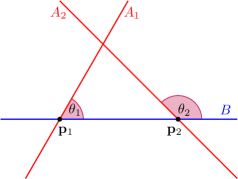
Figure 1. The geometry studied in the paper: One non-convex set, consisting of two lines (red), and another convex set, consisting of one line (blue), with two unique intersection points $\mathbf{p}_{1}$ and $\mathbf{p}_{2}$.

This scenario is intended to be prototypical for the study of the intersection of polygonal sets, which could be approximations of norm-spheres or ellipses. We remark that local convergence for the scenario is already proven in [8]. And while [14] may seem to cover the current scenario as a special case, it does in fact not, as the non-convex set $A$ in this scenario cannot be represented as the graph of a function defined on the set $B$, and because for a global Lyapunov function construction the two isolated attractors $\mathbf{p}_{1}$ and $\mathbf{p}_{2}$ are in conflict with a convexity assumption on the energy function in [14] (both $\mathbf{p}_{i}$ would have to be local minima).

Our main contribution is the construction of a global Lyapunov function for robust $\mathcal{K}\mathcal{L}$-stability in Theorem 5.3. Unlike previous contributions to the Douglas–Rachford convergence analysis based on Lyapunov functions, our construction follows the divide-and-conquer paradigm of re-using known, local Lyapunov functions in our construction of a global Lyapunov function. To this end we use the global Lyapunov functions for the Douglas–Rachford iterations corresponding to the intersection problem between two lines. These are essentially the distance to the intersection point and, in the problem depicted in Fig. 1, they are local Lyapunov functions near each intersection point for the non-convex Douglas–Rachford difference inclusion. The novelty in our contribution is that for a range of problem parameters we can then combine these local Lyapunov functions into a global Lyapunov function for the Douglas–Rachford iteration for the non-convex problem. We can thus deduce that the Douglas–Rachford iteration converges in a non-convex scenario provided certain conditions on the geometry are met. At the same time, we know from extensive numerical experiments that Douglas–Rachford iterations are not guaranteed to converge to a feasible point for all problem parameters. One of the advantages of using Lyapunov functions is the fact that in many cases the existence and properties of a Lyapunov function imply types of convergence which are stronger than point-wise norm convergence. In Corollary 5.6 explicit error bounds for the solutions of perturbed versions of the Douglas–Rachford iteration are given for certain choices of angles $\theta_{1}$, $\theta_{2}$. This means that even if we allow small perturbations of the elements of the Douglas–Rachford iterates, we still obtain uniform convergence on bounded sets.

This paper is organized as follows. Notation is introduced in Section 2. In Section 3 we review known concepts and results from [23] on robust stability with respect to two measures for difference inclusions. This includes the definition of a Lyapunov function as it is commonly used in the modern systems and control literature. The definition of the Douglas–Rachford iteration is recalled in Section 4. In Section 5 we discuss the Douglas–Rachford iteration for two sets $A$ and $B$ with $A$ consisting of two non-parallel lines and $B$ another line, so that the intersection of $A$ and $B$ consists of two points. A technical proof in this section has been postponed to Appendix A. In Section 6 several open problems for further research are formulated, while Section 7 concludes the paper.

Sagemath [29] code in the form of a jupyter notebook is available at [18] for the interested reader to experiment with. This code implements the geometry described above as well as the associated Douglas–Rachford operator.

2. Notation

Denote $\mathbb{R}_{+}\coloneqq[0,\infty[$ and $\mathbb{Z}_{+}\coloneqq\{0,1,2,\dots\}$. By bold letters, like $\mathbf{e}$, $\mathbf{x}$, and $\mathbf{p}$, we denote vectors in the Hilbert space $\mathbb{H}$, and for most of this paper $\mathbb{H}$ is either $\mathbb{R}^{d}$ or $\mathbb{R}^{2}$. Let $B(\mathbf{x},\rho)$ ($B[\mathbf{x},\rho]$) denote the open (closed) ball in $\mathbb{R}^{d}$ centered at $\mathbf{x}$ with radius $\rho$, with respect to the Euclidean norm. Let $\mathbf{e}_{1},\mathbf{e}_{2}$ denote the standard basis vectors in $\mathbb{R}^{2}$, $\mathbf{e}_{1}\coloneqq(1,0)$, $\mathbf{e}_{2}\coloneqq(0,1)$. By $\mathbf{M}_{\theta}$ we denote the rotation matrix

$$\begin{bmatrix}\cos\theta&\sin\theta\\ -\sin\theta~{}&\cos\theta\end{bmatrix}$$

acting on $\mathbb{R}^{2}$. A function $\beta\colon\mathbb{R}_{+}\times\mathbb{R}_{+}\to\mathbb{R}_{+}$ is said to be of class $\mathcal{K}\mathcal{L}$ if for every $t>0$, $\beta(\cdot,t)$ is continuous, strictly increasing, and $\beta(0,t)=0$, and also for every $s\in\mathbb{R}_{+}$, $\beta(s,\cdot)$ is decreasing, and satisfies $\beta(s,t)\stackrel{{\scriptstyle t\to\infty}}{{\longrightarrow}}0$. A function $\varphi\colon\mathbb{R}_{+}\to\mathbb{R}_{+}$ is said to be of class $\mathcal{K}_{\infty}$ if it is continuous, strictly increasing, unbounded, and satisfies $\varphi(0)=0$.

3. The Role of Lyapunov Functions in Robust Stability

In this section we take a detour to recall some known definitions and results from the theory of discrete time dynamical systems and difference inclusions. For more information on the subject the interested reader is referred to [23]. This will serve as a basis for the following section where we will demonstrate that certain instances of the Douglas–Rachford iteration are robustly $\mathcal{K}\mathcal{L}$-stable.

Let $U\subset\mathbb{R}^{d}$, $T\colon U\rightrightarrows U$ be a multi-valued map, and consider the difference inclusion

$$\mathbf{x}_{n+1}\in T\mathbf{x}_{n},\quad n\in\mathbb{Z}_{+}.$$ (1)

A solution to the initial value problem given by the difference inclusion (1) with initial condition $\mathbf{x}_{0}\in U$, which we denote by

$$\phi(\mathbf{x}_{0},\cdot)\colon\mathbb{Z}_{+}\to\mathbb{R}^{d},$$

is a function that satisfies $\phi(\mathbf{x}_{0},0)=\mathbf{x}_{0}$ and

$$\phi(\mathbf{x}_{0},n+1)\in T\big{(}\phi(\mathbf{x}_{0},n)\big{)}$$

for all $n\in\mathbb{Z}_{+}$. Note that for difference inclusions there may well be more than one solution for the same initial value problem. The set of all solutions to (1) is denoted by $\mathcal{S}(\mathbf{x}_{0},T)$. We will also commonly speak of solutions of the difference inclusion (1) and really mean solutions to a corresponding initial value problem that will be clear from the context. A periodic solution $\phi(\mathbf{x}_{0},\cdot)\colon\mathbb{Z}_{+}\to\mathbb{R}^{d}$ is a solution of (1) that is periodic in $n$, i.e., there exists a $K\in\mathbb{Z}_{+}$, $K>1$, such that $\phi(\mathbf{x}_{0},n+K)=\phi(\mathbf{x}_{0},n)$ for all $n\in\mathbb{Z}_{+}$. A periodic orbit is the image of a periodic solution in $\mathbb{R}^{d}$, i.e., the set $\{\phi(\mathbf{x}_{0},n)\colon n\in\mathbb{Z}_{+}\}$. We define several stability properties for the difference inclusion (1).

Definition 3.1 ($\mathcal{K}\mathcal{L}$-stability).

Let $\omega_{1},\omega_{2}\colon\mathbb{R}^{d}\to\mathbb{R}_{+}$ be continuous functions. The difference inclusion (1) is said to be $\mathcal{K}\mathcal{L}$-stable with respect to $(\omega_{1},\omega_{2})$ iff there exists $\beta\in\mathcal{K}\mathcal{L}$ such that for every $\mathbf{x}\in\mathbb{R}^{d}$, every $\phi\in\mathcal{S}(\mathbf{x},T)$ and every $n\in\mathbb{Z}_{+}$,

$$\omega_{1}(\phi(\mathbf{x},n))\leq\beta(\omega_{2}(\mathbf{x}),n).$$

For example, if $\omega_{1}=\omega_{2}$ is just the distance to some set of interest, then $\mathcal{K}\mathcal{L}$-stability says that solutions for any initial conditions will converge to this set with a uniform rate of convergence (which is encoded in $\beta$). To define the stronger notion of robust $\mathcal{K}\mathcal{L}$-stability we need to introduce a few additional concepts. Let $\sigma\colon\mathbb{R}^{d}\to\mathbb{R}_{+}$ and for a set $K\subseteq\mathbb{R}^{d}$ define its dilation with respect to $\sigma$ by

$$K_{\sigma}\coloneqq\bigcup_{\mathbf{x}\in K}B[\mathbf{x},\sigma(\mathbf{x})].$$

Given a map $T\colon\mathbb{R}^{d}\rightrightarrows\mathbb{R}^{d}$, define the $\sigma$-perturbation of $T$ by

$$T_{\sigma}\mathbf{x}\coloneqq\bigcup_{\mathbf{y}\in T(B[\mathbf{x},\sigma(\mathbf{x})])}B[\mathbf{y},\sigma(\mathbf{y})],$$

and let $\mathcal{S}_{\sigma}(\mathbf{x}_{0},T)\coloneqq\mathcal{S}(\mathbf{x}_{0},T_{\sigma})$ be the collection of all solutions to the perturbed difference inclusion $\mathbf{x}_{n+1}\in T_{\sigma}\mathbf{x}_{n}$ with initial condition $\mathbf{x}_{0}$. Notice that if $\sigma\equiv 0$, the constant zero function, then $T_{\sigma}=T$. Finally, given a continuous function $\omega_{1}\colon\mathbb{R}^{d}\to\mathbb{R}_{+}$, define the two sets

$$\mathcal{A}_{\sigma}\coloneqq\mathcal{A}_{\sigma}(T,\omega_{1}) \coloneqq\Big{\{}\mathbf{x}\in\mathbb{R}^{d}\colon\sup_{n\in\mathbb{Z}_{+}}\sup_{\phi\in\mathcal{S}_{\sigma}(\mathbf{x},T)}\omega_{1}(\phi(\mathbf{x},n))=0\Big{\}}$$

and

$$\mathcal{A}\coloneqq\mathcal{A}(T,\omega_{1}) \coloneqq\Big{\{}\mathbf{x}\in\mathbb{R}^{d}\colon\sup_{n\in\mathbb{Z}_{+}}\sup_{\phi\in\mathcal{S}(\mathbf{x},T)}\omega_{1}(\phi(\mathbf{x},n))=0\Big{\}}.$$ (2)

Definition 3.2 (Robust $\mathcal{K}\mathcal{L}$-stability).

Let $\omega_{1},\omega_{2}\colon\mathbb{R}^{d}\to\mathbb{R}_{+}$ be continuous. The difference inclusion (1) is said to be robustly $\mathcal{K}\mathcal{L}$-stable with respect to $(\omega_{1},\omega_{2})$ iff there exists a continuous function $\sigma\colon\mathbb{R}^{d}\to\mathbb{R}_{+}$ such that

1. for all $\mathbf{x}\in\mathbb{R}^{d}\setminus\mathcal{A}$, $\sigma(\mathbf{x})>0$;

2. $\mathcal{A}_{\sigma}=\mathcal{A}$;

3. the difference inclusion $\mathbf{x}_{n+1}\in T_{\sigma}\mathbf{x}_{n}$ is $\mathcal{K}\mathcal{L}$-stable with respect to $(\omega_{1},\omega_{2})$.

Definition 3.3 (Lyapunov function).

Let $\omega_{1},\omega_{2}\colon\mathbb{R}^{d}\to\mathbb{R}_{+}$ be two continuous functions. A function $V\colon\mathbb{R}^{d}\to\mathbb{R}_{+}$ is said to be a Lyapunov function with respect to $(\omega_{1},\omega_{2})$ for the difference inclusion (1) iff there exist $\varphi_{1},\varphi_{2}\in\mathcal{K}_{\infty}$ and $\gamma\in[0,1)$ such that for all $\mathbf{x}\in\mathbb{R}^{d}$,

$$\varphi_{1}(\omega_{1}(\mathbf{x}))\leq V(\mathbf{x})\leq\varphi_{2}(\omega_{2}(\mathbf{x}));$$ (3)

$$\sup_{\mathbf{y}\in T\mathbf{x}}V(\mathbf{y})\leq\gamma V(\mathbf{x});$$ (4)

$$V(\mathbf{x})=0\iff\mathbf{x}\in\mathcal{A},$$ (5)

where $\mathcal{A}$ is defined as in (2).

There is an intimate connection between the stability properties of the difference inclusion (1) and the existence and properties of associated Lyapunov functions. In particular, the following is known.

Theorem 3.4 (Theorem 2.8 in [23]).

Assume that $T\colon\mathbb{R}^{d}\rightrightarrows\mathbb{R}^{d}$ is such that $T\mathbf{x}$ is compact for all $\mathbf{x}\in\mathbb{R}^{d}$. Suppose also that there exists a continuous Lyapunov function on $\mathbb{R}^{d}$ with respect to two continuous functions $\omega_{1}$, $\omega_{2}$. Then the difference inclusion (1) is robustly $\mathcal{K}\mathcal{L}$-stable with respect to $(\omega_{1},\omega_{2})$.

4. The Douglas–Rachford Iteration

For two sets the algorithm can be described as follows. Given a non-empty set $A$ in a Hilbert space $(\mathbb{H},\|\cdot\|)$ and a point $\mathbf{x}\in\mathbb{H}$ denote $d(\mathbf{x},A)\coloneqq\inf_{\mathbf{z}\in A}\|\mathbf{x}-\mathbf{z}\|$. The projection operator $P_{A}\colon\mathbb{H}\rightrightarrows\mathbb{H}$ is given by

$$P_{A}\mathbf{x}\coloneqq\left\{\mathbf{y}\in\mathbb{H}\colon\|\mathbf{x}-\mathbf{y}\|=d(\mathbf{x},A)\right\}$$

and in general it can be multi-valued, but is single-valued if $A$ is non-empty, closed, and convex. Given two closed, non-empty sets $A,B\subseteq\mathbb{H}$, define the Douglas–Rachford operator $T_{A,B}\colon\mathbb{H}\rightrightarrows\mathbb{H}$ by

$$T_{A,B}\coloneqq\frac{I+R_{B}R_{A}}{2},$$

where $I\colon\mathbb{H}\to\mathbb{H}$ is the identity operator, and, given a set $A\subseteq\mathbb{H}$, $R_{A}$ is the reflection operator given by $R_{A}\coloneqq 2P_{A}-I$. The case where $A\cap B\neq\emptyset$ is known as the feasible case. In this paper we will only discuss the feasible case. Specifically, we consider the convergence behavior of the difference inclusion $\mathbf{x}_{n+1}\in T_{A,B}\mathbf{x}_{n}$, with $n\in\mathbb{Z}_{+}$, and $\mathbf{x}_{0}\in\mathbb{H}$, which is known as a Douglas–Rachford iteration of $\mathbf{x}_{0}$.

5. Combining Local Lyapunov Functions to Global Ones

Finding Lyapunov functions is in general the hard part of Lyapunov stability analysis. A divide-and-conquer inspired approach is to try and find Lyapunov functions for simple sub-problems and then combine these into a Lyapunov function for the general case of interest.

In this section we demonstrate that this can be done in a prototypical non-convex scenario for the Douglas–Rachford iteration. In this scenario it is very easy to formulate global Lyapunov functions for the sub-problems (intersections of two lines). In the general version of the problem these functions become then local Lyapunov functions, i.e., they satisfy the descent condition (4) only locally, that is, sufficiently close to a fixed point of the difference inclusion (1). The challenge is then to combine these local Lyapunov functions to one global Lyapunov function, which we demonstrate in Theorem 5.3.

There are several motivations to consider the very simple geometry in this section. Firstly, the case considered here is possibly the simplest non-convex geometry where the Douglas–Rachford iteration converges globally to feasible points for a range of problem parameters. Secondly, it is the first case known to the authors where a global Lyapunov function for the Douglas–Rachford iteration has been constructed from simpler, known local Lyapunov functions. Thirdly, via approximation of circles, ellipses or function graphs through polygons it is not unreasonable to expect that a refined and possibly more localized version of our method could also provide (alternative) Lyapunov function constructions for more involved non-convex geometries like circle and line (cf. [9]), ellipse and line (cf. [10]), or general function graphs and line (cf. [14]). This could open the door to novel sufficient conditions for the convergence of Douglas–Rachford iterations in non-convex scenarios.

5.1. Douglas–Rachford Iteration for Two Intersecting Lines

A case which is elementary and well understood is the case of two straight lines in $\mathbb{R}^{2}$, cf. Fig. 2. For a more general treatment of the intersection of two subspaces we refer the reader to [4].

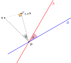
Figure 2. A Douglas–Rachford step for the case of two lines in the plane. Notice that the triangle $\triangle(T_{A,B}\mathbf{x}/\mathbf{p}/\mathbf{x})$ is a right triangle.

The qualitative behavior for this scenario, here presented from a Lyapunov function perspective, is summarized as follows.

Proposition 5.1.

Suppose that $A$ and $B$ are two non-parallel straight lines in $\mathbb{R}^{2}$ which intersect at a point $\mathbf{p}$, cf. Fig. 2. For simplicity we assume $B$ is the $x$-axis. Assume also that the angle from $B$ to $A$ is $\theta\in]0,\pi[$. Then the Douglas–Rachford operator $T_{A,B}$ is single-valued, affine, and is given by

$$T_{A,B}\,\mathbf{x}=\mathbf{p}+\cos\theta\mathbf{M}_{\theta}(\mathbf{x}-\mathbf{p}),$$ (6)

for all $\mathbf{x}\in\mathbb{R}^{2}$. Moreover, the function $V\colon\mathbb{R}^{2}\to[0,\infty)$ given by

$$V(\mathbf{x})\coloneqq\|\mathbf{x}-\mathbf{p}\|^{2},$$ (7)

satisfies (3) with $\varphi_{1}(r)=\varphi_{2}(r)=r^{2}$ and $\omega_{1}(\mathbf{x})=\omega_{2}(\mathbf{x})=\|\mathbf{x}-\mathbf{p}\|$,

$$V(T_{A,B}\mathbf{x})=(\cos^{2}\theta)V(\mathbf{x})<V(\mathbf{x})\quad\text{whenever}\quad\mathbf{x}\neq\mathbf{p}\,,$$ (8)

as well as $V(\mathbf{x})=0$ if and only if $\mathbf{x}=\mathbf{p}$. That is, $V$ is a global Lyapunov function for the Douglas–Rachford iteration, and hence the latter is robustly $\mathcal{KL}$-stable.

Proof.

The result follows from the more general case in [4, Theorem 4.1 and Section 5], up to translation by $\mathbf{p}$, as well as an application of Theorem 3.4. ∎

The existence of a global Lyapunov function guarantees that the Douglas–Rachford iteration converges to a fixed point for any initial condition.

Notice that we chose $V$ to be the squared distance to $\mathbf{p}$. In the control theory literature the choice of a quadratic Lyapunov function is a de facto standard for two reasons. One reason is the chain rule that simplifies the computation of $\frac{d}{dt}V(x(t))=\nabla V(x)f(x)$ in continuous-time dynamics $\dot{x}=f(x)$ at a point $x=x(t)$ without a requirement to compute solutions to a differential equation. The other reason is the added smoothness (compared to simply using the distance) at the reference point, which is beneficial in robustness analysis (especially in continuous-time systems, cf. [22]) and control design (see, e.g., [28]).

5.2. Douglas–Rachford Iteration for Two Lines Intersecting with a Third Line

Now we assume that $A_{1}$, $A_{2}$, are two non-parallel straight lines that each form a positive angle with the positive $x$-axis, and let $A$ be given by $A\coloneqq A_{1}\cup A_{2}$. We assume that $B$ is the $x$-axis, and that we have $A_{1}\cap B\eqqcolon\{\mathbf{p}_{1}\}$, $A_{2}\cap B\eqqcolon\{\mathbf{p}_{2}\}$.

The case when $\mathbf{p}_{1}=\mathbf{p}_{2}$, i.e., all three lines intersect in a single point, is not very different from the discussion in the previous subsection. In fact, it can be shown that the (squared) distance to the common intersection point is a global Lyapunov function for the Douglas–Rachford iteration.

Here we concentrate on the more interesting case when $\mathbf{p}_{1}\neq\mathbf{p}_{2}$. Without loss of generality we may assume $\mathbf{p}_{1}=-\nicefrac{{1}}{{2}}\,\mathbf{e}_{1}$, $\mathbf{p}_{2}=\nicefrac{{1}}{{2}}\,\mathbf{e}_{1}$. Denote by $\theta_{1},\theta_{2}$, the angles of $A_{1},A_{2}$, respectively, with the positive $x$-axis, as denoted in Fig. 1. We assume from here onwards that $0<\theta_{1}\leq\pi/2$ and $\theta_{1}<\theta_{2}<\pi$ (we exclude the cases $\theta_{1}=0$, $\theta_{2}=0$, and $\theta_{1}=\theta_{2}$ since in this case we have parallel lines, or lines that coincide). The following three sets in $\mathbb{R}^{2}$ are of further interest,

$$D_{1} \coloneqq\big{\{}\mathbf{x}\in\mathbb{R}^{2}\colon d(\mathbf{x},A_{1})<d(\mathbf{x},A_{2})\big{\}},$$

$$D_{2} \coloneqq\big{\{}\mathbf{x}\in\mathbb{R}^{2}\colon d(\mathbf{x},A_{1})>d(\mathbf{x},A_{2})\big{\}},\text{ and}$$ (9)

$$D_{3} \coloneqq\big{\{}\mathbf{x}\in\mathbb{R}^{2}\colon d(\mathbf{x},A_{1})=d(\mathbf{x},A_{2})\big{\}},$$

see Fig. 3. It is these sets that determine whether $T_{A,B}$ is multi-valued or singleton-valued, i.e.,

$$T_{A,B}\,\mathbf{x}=\begin{cases}T_{A_{1},B}\,\mathbf{x}&\text{when }\mathbf{x}\in D_{1},\\ T_{A_{2},B}\,\mathbf{x}&\text{when }\mathbf{x}\in D_{2},\\ \big{\{}T_{A_{1},B}\,\mathbf{x},T_{A_{2},B}\,\mathbf{x}\big{\}}&\text{when }\mathbf{x}\in D_{3}.\end{cases}$$ (10)

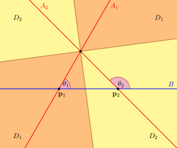
Figure 3. Regions where the Douglas–Rachford operator is single, respectively, multi-valued in the case of two lines (red) and one line (blue). The orange domain is $D_{1}$, the yellow domain is $D_{2}$ (the operator is singleton valued in both cases), and the two brown lines are $D_{3}$ (here the operator has two values).

For $i=1,2$, let $V_{i}\colon\mathbb{R}^{2}\to\mathbb{R}_{+}$ be the functions defined by

$$V_{i}(\mathbf{x})\coloneqq\|\mathbf{x}-\mathbf{p}_{i}\|^{2}.$$ (11)

Following the reasoning of Proposition 5.1, these are now local Lyapunov functions for the Douglas–Rachford iteration

$$\mathbf{x}^{+}\in T_{A,B}\,\mathbf{x},$$ (12)

i.e., if $\mathbf{x}_{0}$ is already sufficiently close to a fixed point $\mathbf{p}_{i}$ then the corresponding sub-level set of $V_{i}$, $\{\mathbf{x}\in\mathbb{R}^{2}:V_{i}(\mathbf{x})\leq V_{i}(\mathbf{x}_{0})\}$, is completely contained in $D_{i}$ and hence invariant under (12). By the decay condition (8) the sequence generated by (12) must converge to $\mathbf{p}_{i}$.

However, if $\|\mathbf{x}_{0}-\mathbf{p}_{i}\|$ is too large for the sub-level set to be completely contained in $D_{i}$, then it is a priori not clear to which point solutions of (12) emerging from $\mathbf{x}_{0}$ converge, or whether they converge at all.

Theorem 5.3 establishes that the globally defined, local Lyapunov functions can indeed be combined to a global Lyapunov function

$$V(\mathbf{x})\coloneqq f\big{(}V_{1}(\mathbf{x}),V_{2}(\mathbf{x})\big{)},$$ (13)

provided a sufficient condition on the angles $\theta_{1}$ and $\theta_{2}$ is met. It is common in Lyapunov stability analysis that conditions are only sufficient and not necessary (see [22] on the concept of converse Lyapunov functions; their existence proofs are usually non-constructive). This global Lyapunov function in turn is a certificate for the global asymptotic stability of the set $\{\mathbf{p}_{1},\mathbf{p}_{2}\}$ of fixed points for the iterative scheme (12), that is, this Lyapunov function establishes among other properties that every solution of (12) converges either to $\mathbf{p}_{1}$ or to $\mathbf{p}_{2}$ for certain configurations of angles $\theta_{1}$ and $\theta_{2}$.

Before we can derive Theorem 5.3, we need to establish a number of technical results that are summarized in the following proposition.

Proposition 5.2.

Given $\rho>0$, let

$$\mathcal{B}_{1}(\rho) \coloneqq\big{\{}\mathbf{x}\in\mathbb{R}^{2}\colon V_{1}(T_{A_{2},B}\mathbf{x})>\rho V_{1}(\mathbf{x})\big{\}}$$

$$\mathcal{B}_{2}(\rho) \coloneqq\big{\{}\mathbf{x}\in\mathbb{R}^{2}\colon V_{2}(T_{A_{1},B}\mathbf{x})>\rho V_{2}(\mathbf{x})\big{\}}$$

denote the sets where function $V_{i}$ increases by at least a factor of $\rho$ along solutions generated by $T_{A_{3-i},B}$.

If $\rho>\cos^{2}\theta_{2}$ then

$$\mathcal{B}_{1}(\rho) =B\left(\mathbf{p}_{1}+\frac{\cos\theta_{2}\sin\theta_{2}}{\rho-\cos^{2}\theta_{2}}\mathbf{e}_{2},\frac{\sqrt{\rho}\sin\theta_{2}}{\rho-\cos^{2}\theta_{2}}\,\right)$$ (14)

and if $$\rho>\cos^{2}\theta_{1}$$ then

$$\mathcal{B}_{2}(\rho) =B\left(\mathbf{p}_{2}-\frac{\cos\theta_{1}\sin\theta_{1}}{\rho-\cos^{2}\theta_{1}}\mathbf{e}_{2},\frac{\sqrt{\rho}\sin\theta_{1}}{\rho-\cos^{2}\theta_{1}}\,\right),$$ (15)

that is, the sets $\mathcal{B}_{i}$ are open balls.

If, moreover, $\rho\geq(1+\sin\theta_{1})(1+\sin\theta_{2})$, then

$$\mathcal{B}_{1}(\rho) \subseteq D_{1},$$ (16)

and

$$\mathcal{B}_{2}(\rho) \subseteq D_{2},$$ (17)

that is, the region where $V_{i}$ increases along solutions generated by $T_{A_{3-i},B}$ is completely contained in $D_{i}$, the set where $T_{A,B}$ is singleton-valued and coincides with $T_{A_{i},B}$.

Observe that $(1+\sin\theta_{1})(1+\sin\theta_{2})>1\geq\cos^{2}\theta_{i}$ for $i=1,2$ in our setting.

The proof of Proposition 5.2 can be found in Appendix A. We can now state the main result of this section. Beforehand we should point out that local convergence of the Douglas–Rachford iteration is already guaranteed by [8]. Our result implies global convergence, despite the complex geometry of the regions of attraction of the individual fixed points, see Fig. 4.

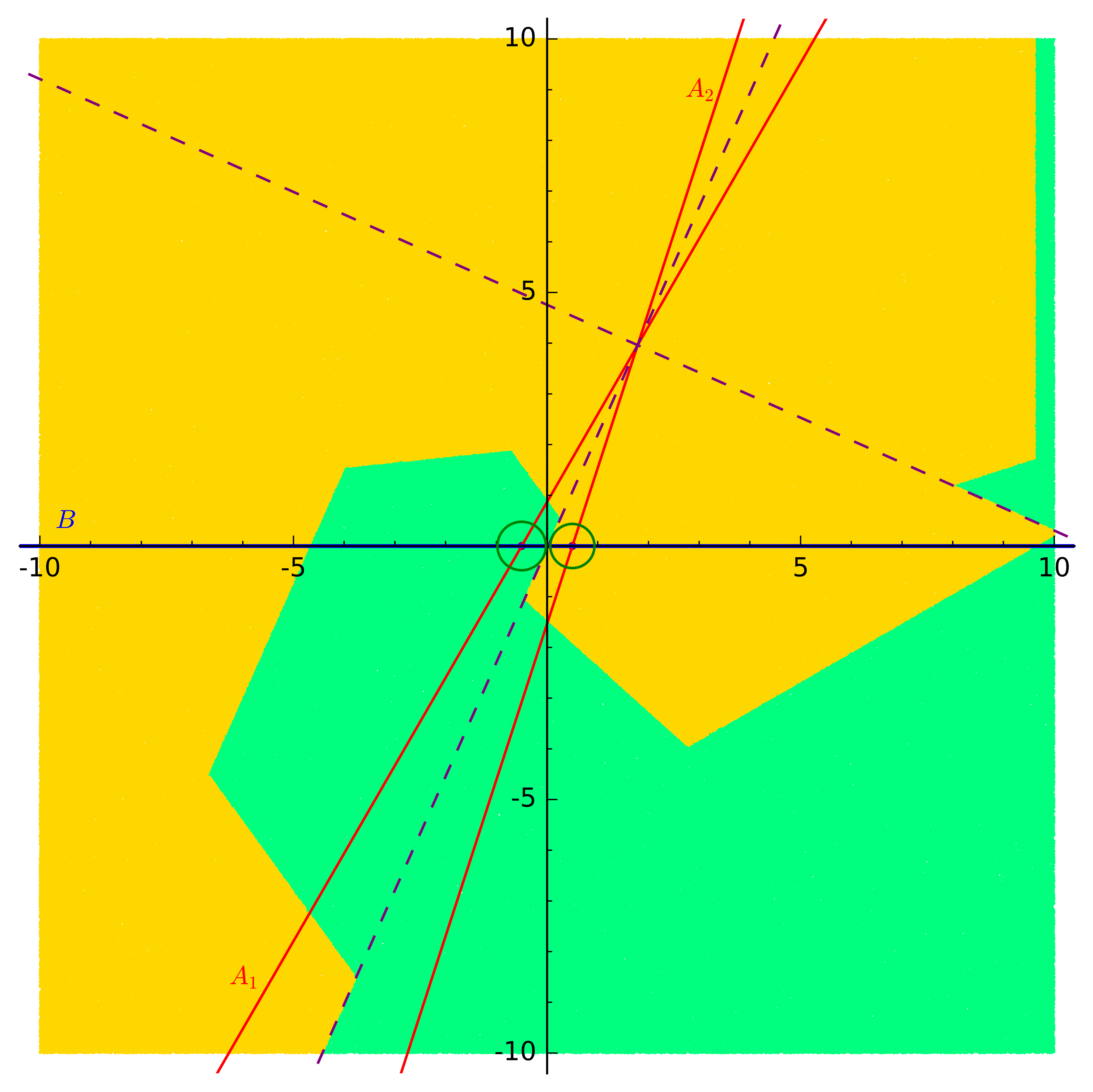
Figure 4. Regions of attraction for the case $\theta_{1}=\pi/3$, $\theta_{2}=2\pi/5$ (for which condition (18) holds). The green circles are centered at $\mathbf{p}_{1}$, $\mathbf{p}_{2}$, with radii $d(\mathbf{p}_{1},D_{3})$, $d(\mathbf{p}_{2},D_{3})$, respectively. The figure is based on a simulation with about 1.5 million data points. For each randomly chosen initial condition a corresponding solution is computed until it enters the inside of one of the regions enclosed by the green circles (which are sub-level sets of $V_{i}$ and completely contained in $D_{i}$, thus invariant under $T_{A,B}$), at which point necessarily the solution converges to the respective intersection point $\mathbf{p}_{i}$. The initial starting point is then colored accordingly.

Theorem 5.3.

Suppose that either $\theta_{1}=\pi/2$, $\theta_{2}=\pi/2$, or that

$$\Big{(}\log\big{(}(1+\sin\theta_{1})(1+\sin\theta_{2})\big{)}\Big{)}^{2}<\log(\cos^{2}\theta_{1})\log(\cos^{2}\theta_{2}).$$ (18)

Then there exist $\alpha\in]0,\infty[$ and $\gamma\in]0,1[$ such that the function $V\colon\mathbb{R}^{2}\to\mathbb{R}_{+}$, defined by

$$V(\mathbf{x})\coloneqq V_{1}(\mathbf{x})^{\alpha}V_{2}(\mathbf{x}),$$ (19)

satisfies

• inequalities (3) with

  $$\omega_{1}(\mathbf{x}) \coloneqq\min\{\|\mathbf{x}-\mathbf{p}_{1}\|,\|\mathbf{x}-\mathbf{p}_{2}\|\}=d(\mathbf{x},A\cap B),$$ (20)

  $$\omega_{2}(\mathbf{x}) \coloneqq\max\{\|\mathbf{x}-\mathbf{p}_{1}\|,\|\mathbf{x}-\mathbf{p}_{2}\|\},$$ (21)

  $$\varphi_{1}(r) \coloneqq\varphi_{2}(r)\coloneqq r^{2\alpha+2};$$ (22)

• the decrease condition

  $$\sup_{\mathbf{y}\in T_{A,B}\mathbf{x}}V(\mathbf{y})\leq\gamma V(\mathbf{x});$$ (23)

• as well as $V(\mathbf{x})=0$ if and only if $\mathbf{x}\in\mathcal{A}\coloneqq\{\mathbf{p}_{1},\mathbf{p}_{2}\}$.

That is, the Douglas–Rachford iteration (12) is robustly $\mathcal{K}\mathcal{L}$-stable with respect to $(\omega_{1},\omega_{2})$.

Proof.

First we establish that there exist $\alpha\in]0,\infty[$ and $\gamma\in]0,1[$ such that

$$\begin{aligned} &&(\cos^{2}\theta_{1})^{\alpha}\big{(}(1+\sin\theta_{1})(1+\sin\theta_{2})\big{)}\phantom{{}^{\alpha}}&\leq\gamma\\ &\text{and}\\ &&(\cos^{2}\theta_{2})\phantom{{}^{\alpha}}\big{(}(1+\sin\theta_{1})(1+\sin\theta_{2})\big{)}^{\alpha}&\leq\gamma.\end{aligned}$$ (24)

Fig. 5 visualizes the relationship between condition (24) and assertion (23) in Theorem 5.3.

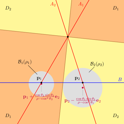
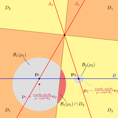
Figure 5. The open balls $\mathcal{B}_{1}(\rho_{1})$, $\mathcal{B}_{2}(\rho_{2})$, defined in Proposition 5.2, for two different choices of $\alpha$ ($\alpha=1$ on the left and $\alpha=3$ on the right), $\theta_{1}=\pi/3$, $\theta_{2}=3\pi/5$ and $\gamma=0.95$. Here $\rho_{1}=\left(\frac{\gamma}{\cos^{2}\theta_{2}}\right)^{1/\alpha}$ and $\rho_{2}=\gamma\left(\frac{1}{\cos^{2}\theta_{1}}\right)^{\alpha}$. In the left figure conditions (24) both hold, while in the right figure the second condition is violated. In the left figure the function $V$ in (19) satisfies (23) everywhere, while in the right figure it does not. The red slice of the open ball in the right figure is the set of points where $V(\mathbf{y})>\gamma V(\mathbf{x})$ for $\mathbf{y}\in T_{A,B}\,\mathbf{x}$.

Inequalities (24) trivially hold if $\theta_{1}=\pi/2$ or $\theta_{2}=\pi/2$, so if $\theta_{1}\neq\pi/2$ and $\theta_{2}\neq\pi/2$ then for condition (24) to hold it is necessary and sufficient that $(\cos^{2}\theta_{1})^{\alpha}\big{(}(1+\sin\theta_{1})(1+\sin\theta_{2})\big{)}<1$ and simultaneously $(\cos^{2}\theta_{2})\big{(}(1+\sin\theta_{1})(1+\sin\theta_{2})\big{)}^{\alpha}<1$, which in turn is equivalent to (18).

The first claim about the functions defined in (20), (21), and (22) satisfying (3) follows by direct computation and the definition (19) of $V$. Obviously the functions $\varphi_{i}$ are of class $\mathcal{K}_{\infty}$ as $\alpha>0$.

From its definition, $V(\mathbf{x})=0$ holds if and only if $\mathbf{x}$ is either $\mathbf{p}_{1}$ or $\mathbf{p}_{2}$. This establishes the third claim.

To establish the second claim, i.e., the decrease condition (23), we have to consider several cases. The first is that $\mathbf{x}\in\{\mathbf{p}_{1},\mathbf{p}_{2}\}$. Then $V(\mathbf{x})$ $=$ $V(T_{A,B}\mathbf{x})=0$ and so (23) holds.

Consider next the case that $\mathbf{x}\in D_{1}\setminus\{\mathbf{p}_{1},\mathbf{p}_{2}\}$. In this case $T_{A,B}=T_{A_{1},B}$ is single-valued by (10). We find

$$V(T_{A,B}\mathbf{x}) = V(T_{A_{1},B}\mathbf{x})=V_{1}^{\alpha}(T_{A_{1},B}\mathbf{x})V_{2}(T_{A_{1},B}\mathbf{x})$$ (25)

$$= \cos^{2\alpha}\theta_{1}V^{\alpha}_{1}(\mathbf{x})V_{2}(T_{A_{1},B}\mathbf{x}),$$

where in the second line we have used (8) of Proposition 5.1. Now, if $\theta_{1}=\nicefrac{{\pi}}{{2}}$ then this reads $V(T_{A,B}\mathbf{x})=0\leq\gamma V(\mathbf{x})$, i.e., the proof for the case $\mathbf{x}\in D_{1}\setminus\{\mathbf{p}_{1},\mathbf{p}_{2}\}$ is complete. So in the following assume that $\theta_{1}\neq\nicefrac{{\pi}}{{2}}$ and note that we also have $V_{1}(\mathbf{x})>0$ since we assumed that $\mathbf{x}\neq\mathbf{p}_{1}$. By way of contradiction, assume now that we have

$$V(T_{A,B}\mathbf{x})>\gamma V(\mathbf{x}).$$ (26)

Then we can arrange (25) into

$$V_{2}(T_{A_{1},B}\mathbf{x}) = \left(\frac{1}{\cos^{2}\theta_{1}}\right)^{\alpha}\cdot\frac{V(T_{A,B}\mathbf{x})}{V_{1}^{\alpha}(\mathbf{x})}\stackrel{{\scriptstyle\eqref{cond bigger}}}{{>}}\left(\frac{1}{\cos^{2}\theta_{1}}\right)^{\alpha}\gamma\cdot\frac{V(\mathbf{x})}{V_{1}^{\alpha}(\mathbf{x})}$$

$$\stackrel{{\scriptstyle\eqref{def V}}}{{=}} \left(\frac{1}{\cos^{2}\theta_{1}}\right)^{\alpha}\gamma V_{2}(\mathbf{x})\stackrel{{\scriptstyle\eqref{the condition}}}{{\geq}}(1+\sin\theta_{1})(1+\sin\theta_{2})V_{2}(\mathbf{x}).$$

An application of Proposition 5.2 lets us deduce that $\mathbf{x}$ must be in $D_{2}$. However, the sets $D_{1}$ and $D_{2}$ are disjoint, so this contradicts our assumptions. This means that the condition $V(T_{A,B}\mathbf{x})>\gamma V(\mathbf{x})$ cannot hold and we have $V(T_{A,B}\mathbf{x})\leq\gamma V(\mathbf{x})$.

The case $\mathbf{x}\in D_{2}\setminus\{\mathbf{p}_{1},\mathbf{p}_{2}\}$ is analogous to the previous one and is thus omitted.

Finally, assume that $\mathbf{x}\in D_{3}\setminus\{\mathbf{p}_{1},\mathbf{p}_{2}\}$. Then by (10) we have $T_{A,B}\mathbf{x}=\big{\{}T_{A_{1},B}\mathbf{x},T_{A_{2},B}\mathbf{x}\big{\}}$. Now, if, by way of contradiction, we assume $V(T_{A_{1},B}\mathbf{x})>\gamma V(\mathbf{x})$ then as before it must follow that $\mathbf{x}\in D_{2}$. If $V(T_{A_{2},B}\mathbf{x})>\gamma V(\mathbf{x})$ then it must follow that $\mathbf{x}\in D_{1}$. In both cases we get $\mathbf{x}\notin D_{3}$, and so neither of these inequalities can hold true. We therefore have in this case $V(T_{A_{1},B}\mathbf{x})\leq\gamma V(\mathbf{x})$ and $V(T_{A_{2},B}\mathbf{x})\leq\gamma V(\mathbf{x})$. We have established that inequality (23), respectively, (4), holds for all $\mathbf{x}\in\mathbb{R}^{2}$.

This establishes that $V$ is indeed a global Lyapunov function for (12) with respect to $(\omega_{1},\omega_{2})$, and by Theorem 3.4 it follows that the difference inclusion (12) is robustly $\mathcal{K}\mathcal{L}$-stable. ∎

Remark 5.4.

Numerical evidence suggests that the region in the parameter space $\{(\theta_{1},\theta_{2})\colon$ $0<\theta_{1}\leq\pi/2$, $\theta_{1}<\theta_{2}<\pi\}$ where all solutions of the Douglas–Rachford iteration converge to $\{\mathbf{p}_{1},\mathbf{p}_{2}\}$ is bigger than the set shown in Fig. 6a, while for some parameter combinations that are outside this set, the Douglas–Rachford iteration may get caught by attractive periodic orbits, cf. Figs. 6b–6d.

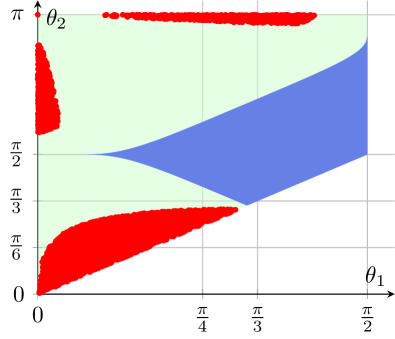
(a) The different regions (red) of parameters for which not all solutions converge to a fixed point of $T_{A,B}$, relative to the admissible parameters (green) and region where (18) holds (blue).

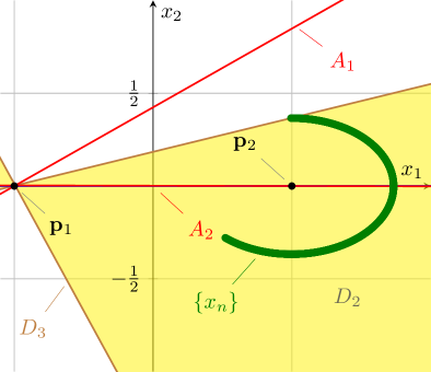
(b) The parameters $\theta_{1}=0.703469$, $\theta_{2}=3.138852$ admit a periodic orbit with period length 1410 containing $\mathbf{x}_{0}=(0.392560,-0.351588)$.

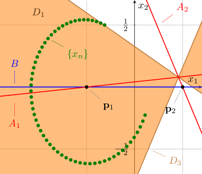
(c) The parameters $\theta_{1}=0.082719$, $\theta_{2}=2.064601$ admit a periodic orbit with period length 58 containing $\mathbf{x}_{0}=(-0.123641,-0.510395)$.

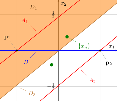
(d) The parameters $\theta_{1}=0.748491$, $\theta_{2}=0.772301$ admit a periodic orbit with period length 2 containing $\mathbf{x}_{0}=(0.101912,0.189275)$.

Figure 6. Numerical experiments. In Fig. 6a we see regions in the $(\theta_{1},\theta_{2})$ plane (restricted to admissible pairs) of parameter combinations for which not all solutions converge to $\{\mathbf{p}_{1},\mathbf{p}_{2}\}$. A sample solution (green) for the lump of points in the top right of the plot is shown in Fig. 6b, as typical solution from the region on the left in Fig. 6c, and one from the region closest to the $\theta_{1}$-axis in Fig. 6d.

Next, we discuss how the order of reflections $R_{A}$ and $R_{B}$ affects the Lyapunov function construction in this paper.

Corollary 5.5.

Under the same assumptions as in Theorem 5.3, the same function $V$ given in (19) satisfies the same conclusions for the Douglas–Rachford iteration given by

$$\mathbf{z}^{+}\in T_{B,A}\,\mathbf{z}.$$

In other words, for this particular geometry the order of the reflections in the Douglas–Rachford iteration does not affect its robust stability.

Proof.

By [7, Proposition 2.5 (i) and Lemma 2.4 (iii)] we have

$$T_{A,B}=R_{B}T_{B,A}R_{B}.$$ (27)

Noting that $R_{B}^{-1}=R_{B}$ and that

$$V_{i}(R_{B}\mathbf{x})=V_{i}(\mathbf{x})$$ (28)

for all $\mathbf{x}\in\mathbb{R}^{2}$ and $i=1,2$, we only need to verify the decrease condition.

From (23) we have that

$$\sup_{\mathbf{y}\in T_{A,B}\mathbf{x}}V(\mathbf{y})\leq\gamma V(\mathbf{x}).$$

Let $\mathbf{w}\in T_{B,A}\mathbf{z}$ with $\mathbf{z}=R_{B}\mathbf{x}$. We want to show that $V(\mathbf{w})\leq\gamma V(\mathbf{z})$.

To this end note that with $\mathbf{y}=R_{B}\mathbf{w}$, we have

$$V(\mathbf{w}) \stackrel{{\scriptstyle\eqref{eq:17}}}{{=}}V(R_{B}\mathbf{w})=V(\mathbf{y}),$$

where clearly $$\mathbf{y}\in R_{B}T_{B,A}R_{B}\mathbf{x}\stackrel{{\scriptstyle\eqref{eq:18}}}{{=}}T_{A,B}\mathbf{x}$$. Hence we continue to estimate

$$\stackrel{{\scriptstyle\eqref{multi decrease V}}}{{\leq}}\gamma V(\mathbf{x})=\gamma V(R_{B}\mathbf{z})\stackrel{{\scriptstyle\eqref{eq:17}}}{{=}}\gamma V(\mathbf{z}).$$

This establishes the decrease condition. All other estimates are the same as in the theorem. ∎

Theorem 5.3 allows us to specify explicitly the convergence behavior of the Douglas–Rachford difference inclusion (12) even in the presence of perturbations. For example, it is possible to prove the following robustness result.

Corollary 5.6.

Under the assumptions of Theorem 5.3, and with $\varepsilon\in]0,1[$ such that $(1+\varepsilon)^{2}\gamma<1$, let

$$\sigma(\mathbf{x})=\big{(}(1+\varepsilon)^{\frac{1}{2(1+\alpha)}}-1\big{)}d(\mathbf{x},A\cap B).$$ (29)

Then for all $\mathbf{x}\in\mathbb{R}^{2}$ and $n\in\mathbb{Z}_{+}$,

$$\sup_{\phi\in\mathcal{S}_{\sigma}(\mathbf{x},T_{A,B})}d(\phi(\mathbf{x},n),A\cap B)\leq\max\{\|\mathbf{x}-\mathbf{p}_{1}\|,\|\mathbf{x}-\mathbf{p}_{2}\|\}\left((1+\varepsilon)^{2}\gamma\right)^{\frac{n}{2\alpha+2}}.$$

The proof of Corollary 5.6 can be found in Appendix B.

6. Perspectives and Open Problems

While the Lyapunov approach for studying asymptotic stability has a long history, its use to study convergence of Douglas–Rachford is very recent. Two main reasons for its success are that, in essence, asymptotic stability implies the existence of a Lyapunov function, and, secondly, that these functions can provide global stability certificates and, in the non-global case, useful estimates on the regions of attraction, i.e., the sets of initial conditions from where the iteration is going to converge. However, several problems are left open for further investigation.

One question concerning Theorem 5.3 is to find a Lyapunov function for a larger region in the $(\theta_{1},\theta_{2})$-domain, cf. Fig. 6a, in order to reduce the conservativeness inherent to the present approach. Notice that in the case where $\theta_{1}\in]0,\pi/2]$ and $\theta_{2}=\pi-\theta_{1}$, the function $V\colon\mathbb{R}^{2}\to\mathbb{R}_{+}$, defined by

$$V(\mathbf{x})\coloneqq\min\{V_{1}(\mathbf{x}),V_{2}(\mathbf{x})\},$$ (30)

satisfies $V(T_{A,B}\mathbf{x})=\cos^{2}\theta_{1}V(\mathbf{x})$. This case is particularly simple, since we have $T_{A_{i},B}D_{i}\subseteq D_{i}$ for $i=1,2$. However, if $V$ is chosen as in (30) then it does not satisfy the decay condition (23) for some of the choices of $\theta_{1}$ and $\theta_{2}$ that satisfy the assumptions of Theorem 5.3.

A natural extension of Theorem 5.3 concerns the study of affine subspaces in higher dimensional spaces, along the lines of [4], which could provide a better intuition for understanding the global convergence of the Douglas–Rachford iteration in more general scenarios.

Yet another question concerns the study of the parameter regions where periodic orbits seem to occur. In numerical experiments these periodic orbits appear to be attracting nearby solutions, so it seems reasonable to conjecture that for the periodic orbits, too, one can find suitable (local) Lyapunov functions and then use these to estimate the corresponding regions of attraction, which are linked to the success rate of the algorithm (ratio of convergent/nonconvergent solutions).

As for robustness, we did not try to give optimal bounds in Corollary 5.6, and there may be room for further improvement.

For us the most interesting question is to construct a Lyapunov function for the case of a polygon and a line, which opens a pathway towards considering even more complex geometries like circle and line or ellipse and lines as limits of polygons, possibly exploiting robustness properties along the way. If we consider the case $\mathbb{H}=\mathbb{R}^{2}$, then at any given point the Douglas–Rachford operator reflects either with respect to two lines or with respect to a line and a point, see Fig. 7. This question requires a better understanding of the Douglas–Rachford operator in the case of multiple lines than we currently have.

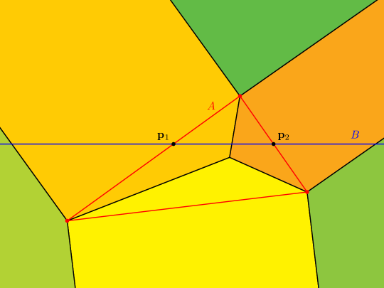
Figure 7. The Douglas–Rachford iteration for a triangle (as a simple polygon) and a straight line. At each point we reflect either with respect to the blue line and one of the red lines (the yellow-orange domains) or with respect to the blue line and one of the red points (the green domains). The black lines are where the map is multi-valued.

The more general case of intersecting non-convex sets that are themselves finite unions of convex sets is understood locally [8]. However, a Lyapunov approach could shed light on the region of attraction and lead to the important insight what other (other than convex) conditions ensure global convergence or at least a large region of attraction, which is of interest in practice.

Lastly, a seemingly simple scenario, that was kindly brought to our attention by Heinz Bauschke, is the convergence behavior in the case of two finite sets. In this case projections are very easy to compute, but the resulting dynamics can be very rich, and essentially nothing is known about the convergence behavior of the Douglas–Rachford iteration to date. This problem, too, once understood, could at a larger scale (many points!) be used to approximate more complex non-convex cases and provide vital insights to their understanding. To put this into the words of the late Jon Borwein: “If there is a problem you don’t understand, there’s a smaller problem within it that you don’t understand. So solve that one first.” The idea here is, of course, that the simpler problem is easier and its solution provides crucial insight into the bigger problem.

7. Conclusions

This paper presents an explicit construction of a Lyapunov function for a Douglas–Rachford iteration in a non-convex setting by combining simple, local Lyapunov functions to a global Lyapunov function. It is discussed how the existence of a global Lyapunov function demonstrates not only global converge to one of the intersection points, but also implies strong stability and robustness properties of the Douglas–Rachford iteration. Several leads for further research directions are provided.

Appendix A Proof of Proposition 5.2.

We begin by establishing condition (14). The proof for condition (15) is essentially the same and thus omitted for brevity.

Establishing Condition (14)

We have by Proposition 5.1 that

$$T_{A_{2},B}\mathbf{x}=\mathbf{p}_{2}+\cos\theta_{2}\mathbf{M}_{\theta_{2}}\left(\mathbf{x}-\mathbf{p}_{2}\right)=\nicefrac{{1}}{{2}}\mathbf{e}_{1}+\cos\theta_{2}\mathbf{M}_{\theta_{2}}\left(\mathbf{x}-\nicefrac{{1}}{{2}}\mathbf{e}_{1}\right).$$

If $\theta_{2}=\nicefrac{{\pi}}{{2}}$ then this simplifies further to $T_{A_{2},B}\mathbf{x}=\mathbf{p}_{2}$, resulting in $V_{1}(T_{A_{2},B}\mathbf{x})=1$. We can hence deduce that

$$1=V_{1}(T_{A_{2},B}\mathbf{x})>\rho V_{1}(\mathbf{x})=\rho\|\mathbf{x}-\mathbf{p}_{1}\|^{2}$$

$$\iff\quad\mathbf{x}\in B(\mathbf{p}_{1},\frac{\sqrt{\rho}}{\rho}).$$ (31)

Now, if $\theta_{2}\neq\nicefrac{{\pi}}{{2}}$ then we have

$$V_{1}(T_{A_{2},B}\mathbf{x})=$ $\left\|T_{A_{2},B}\mathbf{x}-\mathbf{p}_{1}\right\|^{2}=\left\|T_{A_{2},B}\mathbf{x}+\nicefrac{{1}}{{2}}\mathbf{e}_{1}\right\|^{2}\\ =\left\|\mathbf{e}_{1}+\cos\theta_{2}\mathbf{M}_{\theta_{2}}\left(\mathbf{x}-\nicefrac{{1}}{{2}}\mathbf{e}_{1}\right)\right\|^{2}=\left\|\cos\theta_{2}\mathbf{M}_{\theta_{2}}\left(\mathbf{x}-\nicefrac{{1}}{{2}}\mathbf{e}_{1}+S_{\theta_{2}}\mathbf{e}_{1}\right)\right\|^{2}\\ =\cos^{2}\theta_{2}\left\|\mathbf{x}-\nicefrac{{1}}{{2}}\mathbf{e}_{1}+S_{\theta_{2}}\mathbf{e}_{1}\right\|^{2},$$

where $S_{\theta_{2}}\coloneqq\frac{1}{\cos\theta_{2}}\mathbf{M}_{-\theta_{2}}$ satisfies $S_{\theta_{2}}\mathbf{e}_{1}=\mathbf{e}_{1}+\tan\theta_{2}\mathbf{e}_{2}$, and so $-\nicefrac{{1}}{{2}}\mathbf{e}_{1}+S_{\theta_{2}}\mathbf{e}_{1}=\nicefrac{{1}}{{2}}\mathbf{e}_{1}+\tan\theta_{2}\mathbf{e}_{2}$. The inequality $V_{1}(T_{A_{2},B}\mathbf{x})>\rho V_{1}(\mathbf{x})$ is thus equivalent to

$$\cos^{2}\theta_{2}\left\|\mathbf{x}+\nicefrac{{1}}{{2}}\mathbf{e}_{1}+\tan\theta_{2}\mathbf{e}_{2}\right\|^{2}>\rho\left\|\mathbf{x}+\nicefrac{{1}}{{2}}\mathbf{e}_{1}\right\|^{2}.$$

Expanding this gives

$$\cos^{2}\theta_{2}\|\mathbf{x}+\nicefrac{{1}}{{2}}\mathbf{e}_{1}\|^{2}+2\cos^{2}\theta_{2}\tan\theta_{2}\langle\mathbf{x}+\nicefrac{{1}}{{2}}\mathbf{e}_{1},\mathbf{e}_{2}\rangle+\cos^{2}\theta_{2}\tan^{2}\theta_{2}>\rho\left\|\mathbf{x}+\nicefrac{{1}}{{2}}\mathbf{e}_{1}\right\|^{2}$$

or, equivalently,

$$(\rho-\cos^{2}\theta_{2})\left\|\mathbf{x}+\nicefrac{{1}}{{2}}\mathbf{e}_{1}\right\|^{2}-2\cos^{2}\theta_{2}\tan\theta_{2}\left\langle\mathbf{x}+\nicefrac{{1}}{{2}}\mathbf{e}_{1},\mathbf{e}_{2}\right\rangle<\sin^{2}\theta_{2}.$$ (32)

By assumption we have $\rho>\cos^{2}\theta_{2}$. Hence estimate (32) is equivalent to

$$\left\|\mathbf{x}+\nicefrac{{1}}{{2}}\mathbf{e}_{1}\right\|^{2}-2\frac{\cos^{2}\theta_{2}\tan\theta_{2}}{\rho-\cos^{2}\theta_{2}}\left\langle\mathbf{x}+\nicefrac{{1}}{{2}}\mathbf{e}_{1},\mathbf{e}_{2}\right\rangle<\frac{\sin^{2}\theta_{2}}{\rho-\cos^{2}\theta_{2}}.$$

Completing the square gives

$$\left\|\mathbf{x}+\nicefrac{{1}}{{2}}\mathbf{e}_{1}-\frac{\cos\theta_{2}\sin\theta_{2}}{\rho-\cos^{2}\theta_{2}}\mathbf{e}_{2}\right\|^{2} <\frac{\sin^{2}\theta_{2}}{\rho-\cos^{2}\theta_{2}}+\frac{\cos^{2}\theta_{2}\sin^{2}\theta_{2}}{(\rho-\cos^{2}\theta_{2})^{2}}$$

$$=\frac{\rho\sin^{2}\theta_{2}}{(\rho-\cos^{2}\theta_{2})^{2}}.$$ (33)

Since $\theta_{2}\in]0,\pi[$, we have $\sin\theta_{2}>0$ and so (A) is equivalent to

$$\mathbf{x}\in B\left(-\nicefrac{{1}}{{2}}\mathbf{e}_{1}+\frac{\cos\theta_{2}\sin\theta_{2}}{\rho-\cos^{2}\theta_{2}}\mathbf{e}_{2},\frac{\sqrt{\rho}\sin\theta_{2}}{\rho-\cos^{2}\theta_{2}}\,\right).$$

Since $\mathbf{p}_{1}=-\nicefrac{{1}}{{2}}\mathbf{e}_{1}$, this establishes (14), which contains (31) as a special case. $\diamond$

An Auxiliary Lemma

Before we can proceed with the proof of the proposition, we need the following auxiliary result, which provides a characterization of the set $D_{3}$ defined in (5.2). Note that since $A_{1}$ and $A_{2}$ are two non-parallel straight lines, their intersection is a single point.

Lemma A.1.

Let $\mathbf{c}$ be the unique intersection point of $A_{1}$ and $A_{2}$. Then

$$\mathbf{c}=\left(\frac{\sin(\theta_{1}+\theta_{2})}{2\sin(\theta_{2}-\theta_{1})},\frac{\sin\theta_{1}\sin\theta_{2}}{\sin(\theta_{2}-\theta_{1})}\right)$$ (34)

and we have

$$D_{3}=\left\{\mathbf{x}\in\mathbb{R}^{2}\colon\langle\mathbf{x}-\mathbf{c},\mathbf{n}_{1}\rangle=0\right\}\cup\left\{\mathbf{x}\in\mathbb{R}^{2}\colon\langle\mathbf{x}-\mathbf{c},\mathbf{n}_{2}\rangle=0\right\},$$

where $\mathbf{n}_{1}$, $\mathbf{n}_{2}$, are given by

$$\mathbf{n}_{1} =\left(\cos\left(\frac{\theta_{1}+\theta_{2}}{2}\right),\sin\left(\frac{\theta_{1}+\theta_{2}}{2}\right)\right),$$ (35)

$$\mathbf{n}_{2} =\left(\sin\left(\frac{\theta_{1}+\theta_{2}}{2}\right),-\cos\left(\frac{\theta_{1}+\theta_{2}}{2}\right)\right).$$ (36)

Proof.

The line $A_{1}$ is the collection of all points $\mathbf{x}\in\mathbb{R}^{2}$ that satisfy $\langle\mathbf{x},\mathbf{e}_{1}\rangle\sin\theta_{1}$ $-$ $\langle\mathbf{x},\mathbf{e}_{2}\rangle\cos\theta_{1}$ $+$ $\nicefrac{{1}}{{2}}\sin\theta_{1}=0$. Similarly, the line $A_{2}$ is the collection of all points $\mathbf{x}\in\mathbb{R}^{2}$ that satisfy $\langle\mathbf{x},\mathbf{e}_{1}\rangle\sin\theta_{2}-\langle\mathbf{x},\mathbf{e}_{2}\rangle\cos\theta_{2}-\nicefrac{{1}}{{2}}\sin\theta_{2}=0$. Solving these two equations implies that the intersection point $\mathbf{c}$ between $A_{1}$ and $A_{2}$ is indeed given by (34). Now, the (normalized) normal vectors to the lines splitting the angles between $A_{1}$ and $A_{2}$ are given by (35) and (36) and this completes the proof of the auxiliary lemma. ∎

We are now in a position to establish condition (16). The proof of condition (17) follows closely that of condition (16) and is thus omitted for reasons of space.

Establishing Condition (16)

Since the direction vector of $A_{i}$ is $(\cos\theta_{i},\sin\theta_{i})$, $\mathbf{d}_{i}^{\perp}\coloneqq(\sin\theta_{i},-\cos\theta_{i})$ is a normal vector to $A_{i}$ and the distance of a point $Q$ to $A_{i}$ is given by $|\langle Q-\mathbf{p}_{i},\mathbf{d}_{i}^{\perp}\rangle|$. We compute

$$d\left(\mathbf{p}_{1}+\frac{\cos\theta_{2}\sin\theta_{2}}{\rho-\cos^{2}\theta_{2}}\mathbf{e}_{2},A_{1}\right) =\left|\frac{\cos\theta_{1}\cos\theta_{2}\sin\theta_{2}}{\rho-\cos^{2}\theta_{2}}\right|$$ (37)

and

$$d\left(\mathbf{p}_{1}+\frac{\cos\theta_{2}\sin\theta_{2}}{\rho-\cos^{2}\theta_{2}}\mathbf{e}_{2},A_{2}\right) =\left|\frac{\cos^{2}\theta_{2}\sin\theta_{2}}{\rho-\cos^{2}\theta_{2}}+\sin\theta_{2}\right|.$$ (38)

Now, since $\theta_{1}\in]0,\pi/2]$ and $\theta_{2}\in]\theta_{1},\pi[$, we have $|\cos\theta_{1}\cos\theta_{2}|<1$, $\cos^{2}\theta_{i}<1$, $\sin\theta_{2}>0$, and $(1+\sin\theta_{1})(1+\sin\theta_{2})>1$. Since we assumed that $\rho\geq(1+\sin\theta_{1})(1+\sin\theta_{2})$, we have $|\cos\theta_{1}\cos\theta_{2}|<1<\rho$. With these estimates we can bound (37) generously as

$$d\left(\mathbf{p}_{1}+\frac{\cos\theta_{2}\sin\theta_{2}}{\rho-\cos^{2}\theta_{2}}\mathbf{e}_{2},A_{1}\right)<\frac{\rho\sin\theta_{2}}{\rho-\cos^{2}\theta_{2}}$$ (39)

and simplify (38) to

$$d\left(\mathbf{p}_{1}+\frac{\cos\theta_{2}\sin\theta_{2}}{\rho-\cos^{2}\theta_{2}}\mathbf{e}_{2},A_{2}\right)=\sin\theta_{2}\left(\frac{\cos^{2}\theta_{2}}{\rho-\cos^{2}\theta_{2}}+1\right)=\frac{\rho\sin\theta_{2}}{\rho-\cos^{2}\theta_{2}}.$$ (40)

In light of (39) and (40), $A_{1}$ is the closer line to $\mathbf{p}_{1}+\frac{\cos\theta_{2}\sin\theta_{2}}{\rho-\cos^{2}\theta_{2}}\mathbf{e}_{2}$, so it follows that $\mathbf{p}_{1}+\frac{\cos\theta_{2}\sin\theta_{2}}{\rho-\cos^{2}\theta_{2}}\mathbf{e}_{2}\in D_{1}$. Therefore, in order to prove (16), it is enough to show that

$$\frac{\sqrt{\rho}\sin\theta_{2}}{\rho-\cos^{2}\theta_{2}}\leq d\left(\mathbf{p}_{1}+\frac{\cos\theta_{2}\sin\theta_{2}}{\rho-\cos^{2}\theta_{2}}\mathbf{e}_{2},D_{3}\right),$$ (41)

that is, we want the radius of the ball to be smaller than the distance of the center to the boundary of $D_{1}$ (which is exactly $D_{3}$). Now, by the auxiliary Lemma A.1 , we have

$$d\left(\mathbf{p}_{1}+\frac{\cos\theta_{2}\sin\theta_{2}}{\rho-\cos^{2}\theta_{2}}\mathbf{e}_{2},D_{3}\right)=\min_{i=1,2}\left\{\left|\left\langle\mathbf{c}-\mathbf{p}_{1}-\frac{\cos\theta_{2}\sin\theta_{2}}{\rho-\cos^{2}\theta_{2}}\mathbf{e}_{2},\mathbf{n}_{i}\right\rangle\right|\right\}.$$ (42)

By squaring both sides of (41) and using (42) we need to establish that

$$\frac{\rho\sin^{2}\theta_{2}}{(\rho-\cos^{2}\theta_{2})^{2}} \leq\min_{i=1,2}\Bigg{\{} \left(\left\langle\mathbf{c}-\mathbf{p}_{1}-\frac{\cos\theta_{2}\sin\theta_{2}}{\rho-\cos^{2}\theta_{2}}\mathbf{e}_{2},\mathbf{n}_{i}\right\rangle\right)^{2}\Bigg{\}}.$$

Using (34), (35), (36), as well as standard trigonometric identities, the right hand side simplifies to

$$=\min\Bigg{\{} \Bigg{(}\frac{\sin\theta_{2}}{2\sin\left(\frac{\theta_{2}-\theta_{1}}{2}\right)}-\frac{\cos\theta_{2}\sin\theta_{2}}{\rho-\cos^{2}\theta_{2}}\sin\left(\frac{\theta_{1}+\theta_{2}}{2}\right)\Bigg{)}^{2},$$ (43)

$$\Bigg{(}\frac{\sin\theta_{2}}{2\cos\left(\frac{\theta_{2}-\theta_{1}}{2}\right)}+\frac{\cos\theta_{2}\sin\theta_{2}}{\rho-\cos^{2}\theta_{2}}\cos\left(\frac{\theta_{1}+\theta_{2}}{2}\right)\Bigg{)}^{2}\,\Bigg{\}},$$ (44)

so that we need to verify two inequalities, both of which can be simplified further. Starting with (43), we take a common denominator and extract common factors. Using that $0<\theta_{2}<\pi$, $\sin^{2}\theta_{2}>0$, and $\rho>\cos^{2}\theta_{2}$, as well as trusty trigonometric identities, we simplify (43) to

$$\rho^{2}-(2-2\sin\theta_{1}\sin\theta_{2})\rho+\cos^{2}\theta_{1}\cos^{2}\theta_{2}\geq 0.$$ (45)

A similar argument can be made for (44), which simplifies to

$$\rho^{2}-(2+2\sin\theta_{1}\sin\theta_{2})\rho+\cos^{2}\theta_{1}\cos^{2}\theta_{2}\geq 0.$$ (46)

For $\rho>0$, the left hand side of (45) is greater than the left hand side of (46). So it is sufficient to verify that (46) holds.

The roots of the quadratic polynomial in $\rho$ on the left hand side of (46) are $\rho_{1,2}=1+\sin\theta_{1}\sin\theta_{2}\pm(\sin\theta_{1}+\sin\theta_{2})$, so that (46) holds whenever $\rho$ is larger or equal to the larger of the two roots, i.e.,

$$\rho\geq 1+\sin\theta_{1}\sin\theta_{2}+\sin\theta_{1}+\sin\theta_{2}=(1+\sin\theta_{1})(1+\sin\theta_{2}),$$

which establishes (16). $\diamond$

This completes the proof of the proposition.

Appendix B Proof of Corollary 5.6.

We begin with the following lemma.

Lemma B.1.

Let $V\colon\mathbb{R}^{2}\to\mathbb{R}_{+}$ be defined as in (19). Let $\varepsilon\in(0,1)$, and define $\sigma\colon\mathbb{R}_{2}\to\mathbb{R}_{+}$,

$$\sigma(\mathbf{x})=\big{(}(1+\varepsilon)^{\frac{1}{2(1+\alpha)}}-1\big{)}d(\mathbf{x},A\cap B).$$ (47)

Then for every $\mathbf{x}\in\mathbb{R}^{2}$,

$$\sup_{\mathbf{z}\in B[\mathbf{x},\sigma(\mathbf{x})]}V(\mathbf{z})\leq(1+\varepsilon)V(\mathbf{x}).$$

Proof.

Let $\mathbf{z}\in B[\mathbf{x},\sigma(\mathbf{x})]$. We have

$$\|\mathbf{x}-\mathbf{z}\| \leq\left((1+\varepsilon)^{\frac{1}{2(1+\alpha)}}-1\right)d(\mathbf{x},A\cap B)$$

$$=\left((1+\varepsilon)^{\frac{1}{2(1+\alpha)}}-1\right)\min\big{\{}\|\mathbf{x}-\mathbf{p}_{1}\|,\|\mathbf{x}-\mathbf{p}_{2}\|\big{\}},$$ (48)

and so

$$\|\mathbf{z}-\mathbf{p}_{1}\| \leq \|\mathbf{z}-\mathbf{x}\|+\|\mathbf{x}-\mathbf{p}_{1}\|$$ (49)

$$\stackrel{{\scriptstyle\eqref{1st bound rad}}}{{\leq}} \left((1+\varepsilon)^{\frac{1}{2(1+\alpha)}}-1\right)\|\mathbf{x}-\mathbf{p}_{1}\|+\|\mathbf{x}-\mathbf{p}_{1}\|$$

$$= (1+\varepsilon)^{\frac{1}{2(1+\alpha)}}\|\mathbf{x}-\mathbf{p}_{1}\|,$$

and similarly,

$$\|\mathbf{z}-\mathbf{p}_{2}\|\leq(1+\varepsilon)^{\frac{1}{2(1+\alpha)}}\|\mathbf{x}-\mathbf{p}_{2}\|.$$ (50)

Hence,

$$V(\mathbf{z}) = V_{1}^{\alpha}(\mathbf{z})V_{2}(\mathbf{z})=\|\mathbf{z}-\mathbf{p}_{1}\|^{2\alpha}\|\mathbf{z}-\mathbf{p}_{2}\|^{2}$$

$$\stackrel{{\scriptstyle\eqref{z close to p1}\wedge\eqref{z close to p2}}}{{\leq}} (1+\varepsilon)^{\frac{2\alpha+2}{2(\alpha+1)}}\|\mathbf{x}-\mathbf{p}_{1}\|^{2\alpha}\|\mathbf{x}-\mathbf{p}_{2}\|^{2}$$

$$= (1+\varepsilon)V(\mathbf{x}).$$

Since $\mathbf{z}\in B[\mathbf{x},\sigma(\mathbf{x})]$ is arbitrary, the result follows. ∎

Proof of Corollary 5.6.

Let $\mathbf{x}\in\mathbb{R}^{2}$. By the definition of the $\sigma$-perturbation, we have

$$\mathbf{z}\in(T_{A,B})_{\sigma}(\mathbf{x})\iff\mathbf{z}\in\bigcup_{\mathbf{y}\in T_{A,B}(B[\mathbf{x},\sigma(\mathbf{x})])}B[\mathbf{y},\sigma(\mathbf{y})].$$

Therefore, we have

$$\sup_{\begin{subarray}{c}\mathbf{z}\in(T_{A,B})_{\sigma}(\mathbf{x})\end{subarray}}V(\mathbf{z}) = \sup_{\begin{subarray}{c}\mathbf{z}\in B[\mathbf{y},\sigma(\mathbf{y})]\\ \mathbf{y}\in T_{A,B}(B[\mathbf{x},\sigma(\mathbf{x})])\end{subarray}}V(\mathbf{z})$$ (51)

$$\stackrel{{\scriptstyle(\clubsuit)}}{{\leq}} (1+\varepsilon)\sup_{\begin{subarray}{c}\mathbf{y}\in T_{A,B}(B[\mathbf{x},\sigma(\mathbf{x})])\end{subarray}}V(\mathbf{y})$$

$$\stackrel{{\scriptstyle(\spadesuit)}}{{\leq}} (1+\varepsilon)\gamma\sup_{\mathbf{y}\in B[\mathbf{x},\sigma(\mathbf{x})]}V(\mathbf{y})$$

$$\stackrel{{\scriptstyle(\clubsuit)}}{{\leq}} (1+\varepsilon)^{2}\gamma V(\mathbf{x}),$$

where in ($\clubsuit$) we used Lemma B.1 and in ($\spadesuit$) we used (23) in Theorem 5.3. Let $\mathbf{x}\in\mathbb{R}^{2}$ and $\phi\in\mathcal{S}_{\sigma}(\mathbf{x},T_{A,B})$. Then for all $n\in\mathbb{Z}_{+}$, we have by (51),

$$V(\phi(\mathbf{x},n))\leq\left((1+\varepsilon)^{2}\gamma\right)^{n}V(\mathbf{x}).$$ (52)

By Theorem 5.3, $V$ is a Lyapunov function, and in particular satisfies condition (3). Therefore, for $\phi\in\mathcal{S}_{\sigma}(\mathbf{x},T_{A,B})$,

$$d(\phi(\mathbf{x},n),A\cap B)^{2\alpha+2} \stackrel{{\scriptstyle\eqref{eq:9}\wedge\eqref{eq:11}}}{{=}} \varphi_{1}(\omega_{1}(\phi(\mathbf{x},n)))$$

$$\stackrel{{\scriptstyle\eqref{cond omegas}}}{{\leq}} V(\phi(\mathbf{x},n))$$

$$\stackrel{{\scriptstyle\eqref{upper bound iter}}}{{\leq}} \left((1+\varepsilon)^{2}\gamma\right)^{n}V(\mathbf{x})$$

$$\stackrel{{\scriptstyle\eqref{cond omegas}}}{{\leq}} \left((1+\varepsilon)^{2}\gamma\right)^{n}\max\{\|\mathbf{x}-\mathbf{p}_{1}\|,\|\mathbf{x}-\mathbf{p}_{2}\|\}^{2\alpha+2}.$$

Altogether, for all $\mathbf{x}\in\mathbb{R}^{2}$ and $n\in\mathbb{Z}_{+}$,

$$\sup_{\phi\in\mathcal{S}_{\sigma}(\mathbf{x},T_{A,B})}d(\phi(\mathbf{x},n),A\cap B)\leq\max\{\|\mathbf{x}-\mathbf{p}_{1}\|,\|\mathbf{x}-\mathbf{p}_{2}\|\}\left((1+\varepsilon)^{2}\gamma\right)^{\frac{n}{2\alpha+2}}.$$

It is trivial to show that the function $\beta\colon\mathbb{R}_{+}\times\mathbb{R}_{+}\to\mathbb{R}_{+}$ defined by

$$\beta(s,t)=s\left((1+\varepsilon)^{2}\gamma\right)^{\frac{t}{2\alpha+2}}$$

is a $\mathcal{K}\mathcal{L}$-class function. The proof is therefore complete. ∎

Acknowledgements

Ohad Giladi has been supported by ARC grant DP160101537. Björn S. Rüffer has been supported by ARC grant DP160102138. Both authors would like to thank the anonymous referees for their helpful comments.

References

- [1] F. J. Aragón Artacho and J. M. Borwein. Global convergence of a non-convex Douglas-Rachford iteration. J. Global Optim., 57(3):753–769, 2013.
- [2] F. J. Aragón Artacho, J. M. Borwein, and M. K. Tam. Recent results on Douglas-Rachford methods for combinatorial optimization problems. J. Optim. Theory Appl., 163(1):1–30, 2014.
- [3] F. J. Aragón Artacho, J. M. Borwein, and M. K. Tam. Global behavior of the Douglas-Rachford method for a nonconvex feasibility problem. J. Global Optim., 65(2):309–327, 2016.
- [4] H. H. Bauschke, J. Y. Bello Cruz, T. T. A. Nghia, H. M. Phan, and X. Wang. The rate of linear convergence of the Douglas-Rachford algorithm for subspaces is the cosine of the Friedrichs angle. J. Approx. Theory, 185:63–79, 2014.
- [5] H. H. Bauschke, P. L. Combettes, and D. R. Luke. Phase retrieval, error reduction algorithm, and Fienup variants: a view from convex optimization. J. Opt. Soc. Amer. A, 19(7):1334–1345, 2002.
- [6] H. H. Bauschke and M. N. Dao. On the finite convergence of the Douglas-Rachford algorithm for solving (not necessarily convex) feasibility problems in Euclidean spaces. SIAM J. Optim., 27(1):507–537, 2017.
- [7] H. H. Bauschke and W. M. Moursi. On the order of the operators in the Douglas-Rachford algorithm. Optim. Lett., 10(3):447–455, 2016.
- [8] H. H. Bauschke and D. Noll. On the local convergence of the Douglas-Rachford algorithm. Arch. Math. (Basel), 102(6):589–600, 2014.
- [9] J. Benoist. The Douglas-Rachford algorithm for the case of the sphere and the line. J. Global Optim., 63(2):363–380, 2015.
- [10] J. M. Borwein, S. B. Lindstrom, B. Sims, A. Schneider, and M. P. Skerritt. Dynamics of the Douglas-Rachford method for ellipses and -spheres. Set-Valued Var. Anal., 26(2):385–403, 2018.
- [11] J. M. Borwein and B. Sims. The Douglas-Rachford algorithm in the absence of convexity. In Fixed-point algorithms for inverse problems in science and engineering, volume 49 of Springer Optim. Appl., pages 93–109. Springer, New York, 2011.
- [12] M. N. Dao and H. M. Phan. Linear convergence of projection algorithms. arXiv:1609.00341, 9 2016.
- [13] M. N. Dao and H. M. Phan. Linear convergence of the generalized Douglas–Rachford algorithm for feasibility problems. Journal of Global Optimization, 2018.
- [14] M. N. Dao and M. K. Tam. A Lyapunov-type approach to convergence of the Douglas–Rachford algorithm. J . Global Optim., 2018.
- [15] J. Douglas and H. H. Rachford. On the numerical solution of heat conduction problems in two and three space variables. Trans. Amer. Math. Soc., 82:421–439, 1956.
- [16] V. Elser, I. Rankenburg, and P. Thibault. Searching with iterated maps. Proc. Natl. Acad. Sci. USA, 104(2):418–423, 2007.
- [17] O. Giladi. A remark on the convergence of the Douglas-Rachford iteration in a non-convex setting. Set-Valued Var. Anal., 26(2):207–225, 2018.
- [18] O. Giladi and B. S. Rüffer. Accompanying code for the paper “A Lyapunov function construction for a non-convex Douglas–Rachford iteration”, 2017. https://github.com/ogiladi/LyapunovFunDR.
- [19] K. Goebel and W. A. Kirk. Topics in metric fixed point theory, volume 28 of Cambridge Studies in Advanced Mathematics. Cambridge University Press, Cambridge, 1990.
- [20] S. Gravel and V. Elser. Divide and concur: A general approach to constraint satisfaction. Phys. Rev. E, 78:036706, Sep 2008.
- [21] R. Hesse and D. R. Luke. Nonconvex notions of regularity and convergence of fundamental algorithms for feasibility problems. SIAM J. Optim., 23(4):2397–2419, 2013.
- [22] C. M. Kellett. Classical converse theorems in Lyapunov’s second method. Discrete Contin. Dyn. Syst. Ser. B, 20(8):2333–2360, 2015.
- [23] C. M. Kellett and A. R. Teel. On the robustness of -stability for difference inclusions: smooth discrete-time Lyapunov functions. SIAM J. Control Optim., 44(3):777–800, 2005.
- [24] G. Li and T. K. Pong. Douglas-Rachford splitting for nonconvex optimization with application to nonconvex feasibility problems. Math. Program., 159(1-2, Ser. A):371–401, 2016.
- [25] P. L. Lions and B. Mercier. Splitting algorithms for the sum of two nonlinear operators. SIAM J. Numer. Anal., 16(6):964–979, 1979.
- [26] Z. Opial. Weak convergence of the sequence of successive approximations for nonexpansive mappings. Bull. Amer. Math. Soc., 73:591–597, 1967.
- [27] H. M. Phan. Linear convergence of the Douglas-Rachford method for two closed sets. Optimization, 65(2):369–385, 2016.
- [28] E. D. Sontag. Mathematical control theory, volume 6 of Texts in Applied Mathematics. Springer-Verlag, New York, second edition, 1998.
- [29] The Sage Developers. SageMath, the Sage Mathematics Software System (Version 7.x and 8.0), 2017. http://www.sagemath.org.