A hybrid quantum repeater for qudits

Abstract

We present a "hybrid quantum repeater" protocol for the long-distance distribution of atomic entangled states beyond qubits. In our scheme, imperfect noisy entangled pairs of two qudits, i.e., two discrete-variable $d$-level systems, each of, in principle, arbitrary dimension $d$, are initially shared between the intermediate stations of the channel. This is achieved via local, sufficiently strong light-matter interactions, involving optical coherent states and their transmission after these interactions, and optical measurements on the transmitted field modes, especially (but not restricted to) efficient continuous-variable homodyne detections ("hybrid" here refers to the simultaneous exploitation of discrete and continuous variable degrees of freedom for the local processing and storage of entangled states as well as their non-local distribution, respectively). For qutrits we quantify the light-matter entanglement that can be effectively shared through an elementary lossy channel, and for a repeater spacing of up to 10 km we show that the realistic (lossy) qutrit entanglement is even larger than any ideal (loss-free) qubit entanglement. After including qudit entanglement purification and swapping procedures, we calculate the long-distance entangled-pair distribution rates and the final entangled-state fidelities for total communication distances of up to 1280 km. With three rounds of purification, entangled qudit pairs of near-unit fidelity can be distributed over 1280 km at rates of the order of, in principle, 100 Hz.

I Introduction

Long-distance quantum communication is one of the most challenging tasks in practical quantum information. For future quantum networks, the distribution of entanglement between widely separated parties is necessary to make teleportation and secure communication over long distances possible. In practice, however, the direct transmission of quantum information or entangled states is performed by sending light through a lossy quantum channel, which leads to an exponential decay of the success rate or the fidelity. To overcome this problem, quantum repeaters were proposed Briegel1 ; Briegel2 ; Sangouard .

From the perspective of the most recent quantum repeater research, a quantum repeater protocol can be classified into three distinct categories, referred to as quantum repeater generations Optiarchi ; Ultrafast . Though much slower compared to second and third generation quantum repeaters based on quantum error correction of, respectively, local (operation and memory) or, in addition, transmission errors, first generation quantum repeaters are attractive due to their immediate experimental feasibility (however, for a fairly practical approach to a third generation quantum repeater, see Ewert1 ; Ewert2 ). In first generation quantum repeaters, by means of entanglement swapping swap , the distribution of long-distance entanglement is achieved via initial short-distance entanglement distributions. Hence, for the realization of first generation quantum repeater schemes, the heralded generation of short-distance entanglement and the availability of quantum memories are essential prerequisites.
A prominent instance of a first generation quantum repeater scheme is the well-known DLCZ protocol DLCZ which uses atomic ensembles as quantum memories and single photons with linear optics for entanglement distribution and swapping. A remarkable feature of the DLCZ scheme is that the so-called purification of entanglement, turning imperfect mixed entangled states into purer (in principle, perfect) versions of entangled states, is built into the process of entanglement distribution and swapping (purifying the entangled atomic ensembles from the effects of transmission and memory losses, respectively). Otherwise, in a standard first generation quantum repeater Briegel1 ; Briegel2 , quantum error detection must be included via additional rounds of entanglement purification acting on two or more copies of entangled states and employing local quantum logic (together with two-way classical communication). Second generation schemes use quantum error correction against memory errors, while in third generation quantum repeaters no memories are necessary Munro , since, for example, suitably encoded quantum information is directly sent through the channel Ultrafast ; Optiarchi ; Ewert1 ; Ewert2 . A conceptually distinct version of such a loss-error-correction-based repeater is the all-optical scheme of Azuma et al. Azuma based on the distribution of entangled cluster states. This scheme also relies on sufficiently fast feedforward operations (as opposed to the all-optical scheme of Ewert1 ; Ewert2 ).
All experimental demonstrations to date are for elements of a first generation repeater, although light-matter interfaces and/or memories are still too inefficient to exceed the bounds Takeoka ; Pirandola of repeaterless quantum communication (or to even scale up a repeater to really large distances). In fact, almost all quantum memories that have been demonstrated so far perform worse compared to a simple optical fiber loop Cho .
A suitable first generation "hybrid quantum repeater" (HQR) protocol for the distribution of atomic qubit-qubit entanglement was given in HQR ; Bright ; Ladd . Similar to other hybrid quantum information processing schemes HybridQIP , this protocol combines the advantages of discrete and continuous variable quantum states. Atomic two-level systems with long coherence time serve as quantum memories while optical coherent states are used to generate the initial entanglement between the atoms using dispersive light-matter interactions and, in particular, highly efficient homodyne measurements. Employing such Gaussian measurements and Gaussian states as the initial resources appears very attractive from a practical point of view compared to repeater schemes based on the generation and detection of single photons. A particular experimental approach to this scheme, based on ions, was considered in Pfister . Another, similar HQR protocol can be found in Brask and a recent hybrid approach to entanglement swapping using coherent states and linear optics is presented in Jeongswap .
On the fundamental level, higher-dimensional quantum systems of dimension $d$, so called qudits, do not only play an important role in closing of the detection loophole in Bell test experiments violation1 ; violation2 . In addition, it has been shown in Cerf that qudits lead to an increase in data transfer and especially to a higher security in quantum key distribution (QKD) Scarani compared to schemes involving only qubits Twist . One possibility to realize such improved schemes is the initial distribution of high-dimensional entanglement using correspondingly high-dimensional quantum repeaters, which is the topic of this paper . Despite the many existing works on qubit quantum repeaters, rather little attention has been paid to qudit quantum repeaters aiming at the long-distance-distribution of qudit entanglement and information.
In this paper, we generalize the HQR protocol for the distribution of qubit-qubit entanglement HQR ; Bright to the case of qudit-qudit entanglement, i.e., bipartite states of multilevel systems. The structure of the paper is as follows: in Sec. II, we review the HQR protocol for the qubit case and adapt it to our later generalization for qudits. In Sec. III, we generalize this scheme to the case of three-level systems (qutrits). After proposing a generalized dispersive qutrit-light interaction, we discuss the process of entanglement generation in elementary links using this interaction. We consider both homodyne detection and unambiguous state discrimination (USD) for the measurement on the light mode. Including entanglement purification for the initial qutrit-qutrit entangled states, we calculate the final rates and fidelities for our generalized entanglement distribution scheme in various scenarios. Based on these results, in Sec. IV we discuss a generalization to arbitrarily dimensional quantum systems before we conclude in Sec. V.

II Hybrid quantum repeater for qubits

The physical setup for a qubit HQR is as follows: the qubit is represented by the two spin states $|0\rangle$ and $|1\rangle$ of an atomic electron. The atom is placed into a cavity and the electronic spin interacts with a bright coherent-state light pulse. The situation at hand is theoretically described by the Jaynes-Cummings model in the limit of large detuning JC , i.e., the probe pulse and the cavity are in resonance, but both are detuned from the resonance frequency of the electronic transition.
The interaction Hamiltonian in this model reads $H_{int}^{(2)}=\hbar g\sigma_{z}a^{\dagger}a$, where $\sigma_{z}=-\frac{1}{2}|0\rangle\langle 0|+\frac{1}{2}|1\rangle\langle 1|$ corresponds to a Pauli operator on the spin state and $a^{\dagger}a$ is the photon number operator of the light mode. Furthermore, the parameter $g$ describes the strength of the spin-light coupling.
Based on this interaction Hamiltonian, the corresponding unitary transformation is given by $U_{2}(\theta)=\exp(i\theta\sigma_{z}a^{\dagger}a)$ (with an effective interaction time $\theta=gt$) and, up to an unconditional phase shift of the mode by $e^{i\theta/2}$, acts on the spin-light system effectively as a controlled phase rotation, i.e.

$$U_{2}(\theta)[(|0\rangle+|1\rangle)\otimes|\alpha\rangle]=|0\rangle|\alpha\rangle+|1\rangle|\alpha e^{i\theta}\rangle.$$ (1)

In the literature, this interaction is also known as dispersive interaction gerry . For the generalization that we are aiming at, we consider the case $\theta=\pi$, corresponding to a strong interaction resulting in coherent states $|\pm\alpha\rangle$ on the light mode.
The repeater protocol now works as follows: the matter system is prepared in the state $|0\rangle+|1\rangle$ and interacts dispersively with a single-mode coherent state $|\alpha\rangle$ (referred to as "qubus") as described by Eq. (1). Note that this leads to a pure (effectively qubit-qubit) entangled state between the light mode and the matter system.
The light mode is then sent through an optical channel where it inevitably suffers from photon loss. The photon loss can be modeled by mixing the light mode with a vacuum state at a beam splitter with transmittance $\gamma$, where $1-\gamma$ is related to the loss probability of a single photon. It is also related to the optical propagation distance $L$, i.e., $\gamma=\exp\left(-\frac{L}{L_{att}}\right)$ with the attenuation length $L_{att}\approx 22\leavevmode\nobreak\ \text{km}$ for photons at telecom wavelength.
After applying the beam splitter, the total pure state of the matter system, the qubus light mode and the loss mode reads as

$$\frac{1}{\sqrt{2}}(|0\rangle|\sqrt{\gamma}\alpha\rangle|\sqrt{1-\gamma}\alpha\rangle+|1\rangle|-\sqrt{\gamma}\alpha\rangle|-\sqrt{1-\gamma}\alpha\rangle).$$ (2)

The relevant joint state of the matter system and the light mode is obtained by tracing out the loss mode. Since the coherent states $|\alpha\rangle$ and $|-\alpha\rangle$ are not orthogonal, it is useful to transform these into an orthogonal basis. A suitable orthogonal basis in this case is the basis of even and odd cat states (throughout we assume $\alpha\in\mathbb{R}$),

$$|u\rangle =\frac{1}{\sqrt{N_{u}(\alpha)}}(|\alpha\rangle+|-\alpha\rangle),$$ (3)

$$|v\rangle =\frac{1}{\sqrt{N_{v}(\alpha)}}(|\alpha\rangle-|-\alpha\rangle),$$ (4)

with normalization constants $N_{u}(\alpha)=2(1+e^{-2\alpha^{2}})$ and $N_{v}(\alpha)=2(1-e^{-2\alpha^{2}})$. Expressed in this basis, one has

$$|\alpha\rangle=\frac{1}{2}(\sqrt{N_{u}(\alpha)}|u\rangle+\sqrt{N_{v}(\alpha)}|v\rangle),$$ (5)

$$|-\alpha\rangle=\frac{1}{2}(\sqrt{N_{u}(\alpha)}|u\rangle-\sqrt{N_{v}(\alpha)}|v\rangle).$$ (6)

After tracing out the loss mode in this basis, the resulting state of the matter system and the qubus light mode becomes

$$\rho_{out} =\frac{N_{u}(\sqrt{1-\gamma}\alpha)}{4}$$ (7)

$$\times\left[\frac{1}{\sqrt{2}}\left(|0\rangle|\sqrt{\gamma}\alpha\rangle+|1\rangle|-\sqrt{\gamma}\alpha\rangle\right)\right]\times H.c.$$

$$+\frac{N_{v}(\sqrt{1-\gamma}\alpha)}{4}$$

$$\times\left[\frac{1}{\sqrt{2}}\left(|0\rangle|\sqrt{\gamma}\alpha\rangle-|1\rangle|-\sqrt{\gamma}\alpha\rangle\right)\right]\times H.c.$$

This is a mixed entangled state between the matter system (the atomic qubit) and the qubus. To study the entanglement of such a state and also for later purposes, it is most convenient to use directly the ${|\widetilde{u}\rangle,|\widetilde{v}\rangle}$-basis on the light mode , where $\sim$ refers to the basis vectors in Eqs. (3) and (4) with damped amplitudes $\sqrt{\gamma}\alpha$.
In addition, a basis change on the matter qubit system into the conjugate X-basis, $|\widetilde{0}\rangle=\frac{1}{\sqrt{2}}(|0\rangle+|1\rangle)$ and $|\widetilde{1}\rangle=\frac{1}{\sqrt{2}}(|0\rangle-|1\rangle)$, gives the expression

$$\rho_{out} =\frac{N_{u}(\sqrt{1-\gamma}\alpha)}{4}\left[\frac{1}{2}\left(\sqrt{N_{u}(\sqrt{\gamma}\alpha)}|\widetilde{0}\rangle|\widetilde{u}\rangle\right.\right.$$ (8)

$$+\left.\left.\sqrt{N_{v}(\sqrt{\gamma}\alpha)}|\widetilde{1}\rangle|\widetilde{v}\rangle\right)\right]\times H.c.$$

$$+\frac{N_{v}(\sqrt{1-\gamma}\alpha)}{4}\left[\frac{1}{2}\left(\sqrt{N_{u}(\sqrt{\gamma}\alpha)}|\widetilde{1}\rangle|\widetilde{u}\rangle\right.\right.$$

$$+\left.\left.\sqrt{N_{v}(\sqrt{\gamma}\alpha)}|\widetilde{0}\rangle|\widetilde{v}\rangle)\right)\right]\times H.c.,$$

which represents the state in Eq. (7) in suitable binary orthogonal bases for both the matter system and the qubus. Note that this does not change the entanglement properties of the state since any entanglement measure is invariant under local basis changes Plenio ; Guehne ; Horodeckireview . Also note that this matter-light qubit-qubus entangled state effectively remains an entangled qubit-qubit state, since the two initial coherent states of the qubus span a two-dimensional qubit space and because individual coherent states remain pure after a loss channel.
After traveling through an optical fiber over the distance $L_{0}$, the light mode interacts dispersively with a second matter qubit system, also prepared in the state $|0\rangle+|1\rangle$, but this time with the inverse angle, $\theta=-\pi$.
The joint tripartite state, written in the same basis as in Eq. (7), then becomes

$$\rho_{out} =\frac{N_{u}(\sqrt{1-\gamma}\alpha)}{4}|C_{0}\rangle\langle C_{0}|$$ (9)

$$+\frac{N_{v}(\sqrt{1-\gamma}\alpha)}{4}|C_{1}\rangle\langle C_{1}|,$$

where

$$|C_{0}\rangle=\frac{1}{\sqrt{2}}(|\phi^{+}\rangle|\sqrt{\gamma}\alpha\rangle+|\psi^{+}\rangle|-\sqrt{\gamma}\alpha\rangle),$$ (10)

and

$$|C_{1}\rangle=\frac{1}{\sqrt{2}}(|\phi^{-}\rangle|\sqrt{\gamma}\alpha\rangle+|\psi^{-}\rangle|-\sqrt{\gamma}\alpha\rangle).$$ (11)

Here we introduced the qubit Bell states

$$|\phi^{\pm}\rangle =\frac{1}{\sqrt{2}}(|00\rangle\pm|11\rangle),$$ (12)

$$|\psi^{\pm}\rangle =\frac{1}{\sqrt{2}}(|10\rangle\pm|01\rangle).$$

The component $|C_{0}\rangle$ in Eq. (9) is the desired target component, whereas $|C_{1}\rangle$ is the loss component that vanishes in the loss-free case. Indeed, for $\gamma\rightarrow 1$, one observes $N_{u}(0)=4$ and $N_{v}(0)=0$ such that in this case the corresponding output density operator $\rho_{out}=|C_{0}\rangle\langle C_{0}|$ represents a pure state. Opposed to the original HQR for qubits Bright , here every term in $|C_{0}\rangle$ contains matter two-qubit entanglement because of our choice $\theta=\pm\pi$. This choice will enable us later to obtain a natural generalization to qudits.
To achieve the goal of distributing entanglement between the two separated matter systems over the distance $L_{0}$, the final step is a measurement on the light mode, for instance, by homodyne detection.
Unlike in the original HQR protocol Bright where the dispersive interaction is assumed to be weak (and hence a p-homodyne detection is ultimately preferred over an $x$-homodyne detection with, respectively, state distinguishabilities $\sim\alpha\theta$ versus $\alpha\theta^{2}$ for small but otherwise unfixed theta), a suitable detection scheme in our case for "strong" and fixed $\theta=\pm\pi$ is a measurement of the quadrature $\hat{x}=\frac{1}{2}(a+a^{\dagger})$ instead of $\hat{p}=\frac{1}{2i}(a-a^{\dagger})$.
The position distribution of coherent states with complex amplitude $\beta$ can be obtained by the square of their position wave functions,

$$|\psi_{\beta}(x)|^{2}=\sqrt{\frac{2}{\pi}}\exp\left(-2(x-\operatorname{Re}(\beta))^{2}\right).$$ (13)

Because of the finite overlap of the coherent states $|\sqrt{\gamma}\alpha\rangle$ and $|-\sqrt{\gamma}\alpha\rangle$, it is impossible to perfectly distinguish these states and an error due to this non-orthogonality has to be taken into account. Based on Eq. (13), it is obvious that $|\sqrt{\gamma}\alpha\rangle$ and $|-\sqrt{\gamma}\alpha\rangle$ have Gaussian position distributions around $\sqrt{\gamma}\alpha$ and $-\sqrt{\gamma}\alpha$, respectively. It is therefore useful to assign the result of the x-measurement to one of three possible windows.
The first window is $w_{0}=[\sqrt{\gamma}\alpha-\Delta,\infty]$ with $\sqrt{\gamma}\alpha>\Delta>0$. If the measurement result falls into this range, then the light mode is effectively projected onto $|\sqrt{\gamma}\alpha\rangle$. Note that this is an approximate projection due to the non-orthogonality, i.e., the resulting state is still a superposition of $|\phi^{+}\rangle$ and $|\psi^{+}\rangle$ in the first component, while the weight of $|\psi_{+}\rangle$ can be reduced by increasing the value of $\sqrt{\gamma}\alpha$. The same is true in the second component for $|\phi^{-}\rangle$ and $|\psi^{-}\rangle$.
As for the second window, we define $w_{1}=[-\infty,-\sqrt{\gamma}\alpha+\Delta]$, which is symmetric to $w_{0}$ and therefore represents the approximate projection on $|-\sqrt{\gamma}\alpha\rangle$. Unlike $w_{0}$, one has now $|\psi^{\pm}\rangle$ as the dominant terms in the superpositions in the two components. It is again true that the non-dominant term in the superposition can be made arbitrarily small by increasing $\sqrt{\gamma}\alpha$. A third window, $w_{2}$, can be defined in between $w_{0}$ and $w_{1}$, and a measurement result in this range will be considered as a failure event to be discarded (see Fig. 1).

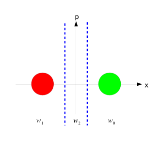
Figure 1: Phase space representation of two coherent states $|\sqrt{\gamma}\alpha\rangle$ and $|-\sqrt{\gamma}\alpha\rangle$ to be distinguished by homodyne detection. The measurement window $w_{2}$ includes all failure events that are discarded.

Useful figures of merit for the performance of this entanglement distribution scheme are the success probabilities for the two non-failure windows $w_{0}$ and $w_{1}$ as well as the fidelity of the corresponding target state in the first component. As the fidelity, we define the overlap of the maximally entangled Bell states $|\phi^{+}\rangle$ $(w_{0})$ or $|\psi^{+}\rangle$ $(w_{1})$ with the mixed state in Eq. (9) after the corresponding homodyne measurement outcome.
The success probability for a measurement result to fall into the first window reads

$$p_{w_{0}}=\frac{1}{2}\int\limits_{\sqrt{\gamma}\alpha-\Delta}^{\infty}dx(|\psi_{\sqrt{\gamma}\alpha}(x)|^{2}+|\psi_{-\sqrt{\gamma}\alpha}(x)|^{2}).$$ (14)

For the second window, we have

$$p_{w_{1}}=\frac{1}{2}\int\limits_{-\infty}^{-\sqrt{\gamma}\alpha+\Delta}dx(|\psi_{\sqrt{\gamma}\alpha}(x)|^{2}+|\psi_{-\sqrt{\gamma}\alpha}(x)|^{2}),$$ (15)

which equals $p_{w_{0}}$ for symmetry reasons. The same holds true for the two fidelities,

$$F_{w_{0}} =F_{w_{1}}$$ (16)

$$=\frac{N_{u}(\sqrt{1-\gamma}\alpha)}{4}$$

$$\times\frac{\int\limits_{-\infty}^{-\sqrt{\gamma}\alpha+\Delta}dx|\psi_{\sqrt{\gamma}\alpha}(x)|^{2}}{\int\limits_{-\infty}^{-\sqrt{\gamma}\alpha+\Delta}dx(|\psi_{\sqrt{\gamma}\alpha}(x)|^{2}+|\psi_{-\sqrt{\gamma}\alpha}(x)|^{2})}.$$

The formulae for the fidelities and the success probabilities imply the crucial dependence of the performance on the choice of $\Delta$ and $\sqrt{\gamma}\alpha$: if we choose $\Delta=\Delta_{0}:=\sqrt{\gamma}\alpha$, then we have no failure window and every measurement result is assigned to one of the two coherent states $|\pm\sqrt{\gamma}\alpha\rangle$. The corresponding success probability equals unity at the expense of a rather low fidelity.
With $\Delta<\Delta_{0}$, the success probability is clearly less than unity and the fidelity increases correspondingly.
In general, the fidelity drops for too small $\sqrt{\gamma}\alpha$ due to the non-orthogonality and thus indistinguishability of the coherent states $|\pm\sqrt{\gamma}\alpha\rangle$. The overall effect becomes manifest in bit-flip errors in the target Bell states. Though leading to near-orthogonality, large amplitudes $\sqrt{\gamma}\alpha$ result in a near-equal mixture of the state in Eq. (9) which then, after a near-deterministic discrimination, consists of one of the two possible Bell states in the first component and its phase-flipped version in the second component. This state therefore has very low entanglement and hence is of limited practical interest. So the task is to find a regime of $\alpha$ and distances $L_{0}$ such that both reasonable fidelities and success probabilities can be obtained.
Besides homodyne detection, unambiguous state discrimination (USD) has been considered for hybrid quantum repeaters in the literature HQR . The advantage here is that the effects originating from the finite overlaps of the coherent states no longer appear in the fidelity thanks to an error-free state discrimination. The corresponding effects solely influence the success probabilities depending on the weights of the inconclusive discrimination results. Two-state USD for coherent states $|\pm\sqrt{\gamma}\alpha\rangle$ is well-known and can be optimally performed via a single beam splitter and on-off detections BanaszekUSD .
Further steps in the original repeater protocol address the purification of the mixed state in Eq. (9) after homodyne detection and entanglement swapping on the matter system or via the qubus to distribute the generated entanglement over longer distances.
For more details, see e.g. HQR .

III Hybrid quantum repeater for qutrits

III.1 Dispersive light-matter interaction

The dispersive interaction (see Eq. (1)) lies at the heart of the HQR for qubits and therefore, as a first step to extend this repeater scheme to qutrits, a generalization of the dispersive interaction to the qutrit case is necessary.
In analogy to the dispersive interaction for qubits, we define the qutrit-qubus interaction Hamiltonian as

$$H_{int}^{(3)}=\hbar gS_{z}^{(3)}a^{\dagger}a,$$ (17)

where the operator $S_{z}^{(3)}$ acts on the qutrit basis states $|0\rangle$, $|1\rangle$ and $|2\rangle$ as

$$S_{z}^{(3)}|0\rangle =-1\cdot|0\rangle,$$ (18)

$$S_{z}^{(3)}|1\rangle =0\cdot|1\rangle,$$

$$S_{z}^{(3)}|2\rangle =1\cdot|2\rangle.$$

The matter system could be, for example, realized by a spin-1 particle where the basis states are the eigenstates with the corresponding magnetic quantum numbers, $m_{z}=-1,0,1$. Such a spin realization of a qutrit has been demonstrated in the framework of nuclear magnetic resonance (NMR) for various applications NMR1 ; NMR2 .
Similar to the qubit case, the corresponding unitary transformation is $U_{3}(\theta)=\exp\left(i\theta S_{z}^{(3)}a^{\dagger}a\right)$, which again corresponds to a conditional phase rotation on the light-matter system (up to an unconditional phase shift of the qubus mode by $e^{i\theta}$), i.e.,

$$U_{3}(\theta)(|0\rangle+|1\rangle+|2\rangle)\otimes|\alpha\rangle=|0\rangle|\alpha\rangle+|1\rangle|\alpha e^{i\theta}\rangle+|2\rangle|\alpha e^{2i\theta}\rangle.$$ (19)

For our purposes, we will choose $\theta=\frac{2\pi}{3}$ to obtain a rather strong dispersive interaction.

III.2 Loss-free case

The qutrit hybrid repeater protocol works in complete analogy to the qubit case. To illustrate the concept, we first omit photon losses in the optical fiber and assume a noiseless quantum channel.
The repeater protocol works as follows: First, the matter system is initiated in the state $\frac{1}{\sqrt{3}}(|0\rangle+|1\rangle+|2\rangle)$ and interacts with a light mode in a coherent state $|\alpha\rangle$ via the qutrit dispersive interaction with $\theta=\frac{2\pi}{3}$. This results in the entangled matter-qubus state

$$\frac{1}{\sqrt{3}}\left(|0\rangle|\alpha\rangle+|1\rangle|\alpha e^{\frac{2\pi i}{3}}\rangle+|2\rangle|\alpha e^{-\frac{2\pi i}{3}}\rangle\right).$$ (20)

The light mode is then sent to a second matter system, separated from the first one by a distance $L_{0}$ and also prepared in the state $\frac{1}{\sqrt{3}}(|0\rangle+|1\rangle+|2\rangle)$. The incoming light mode interacts dispersively with the second matter system, but this time with the reverse angle $\theta=-\frac{2\pi}{3}$. The resulting pure state is

$$\frac{1}{\sqrt{3}} \left(\frac{1}{\sqrt{3}}(|00\rangle+|11\rangle+|22\rangle)|\alpha\rangle\right.$$ (21)

$$+\frac{1}{\sqrt{3}}(|02\rangle+|10\rangle+|21\rangle)|\alpha e^{\frac{2\pi i}{3}}\rangle$$

$$+\left.\frac{1}{\sqrt{3}}(|01\rangle+|12\rangle+|20\rangle)|\alpha e^{-\frac{2\pi i}{3}}\rangle\right).$$

To keep the notation short and also for later purposes, it it useful to define the set of maximally entangled qutrit Bell states,

$$|\phi_{kj}\rangle=\frac{1}{\sqrt{3}}\sum\limits_{m=0}^{2}\exp\left(\frac{2\pi ikm}{3}\right)|m,m\ominus j\rangle,$$ (22)

where $"\ominus"$ denotes subtraction modulo 2. Eq. (21) can therefore be rewritten as

$$\frac{1}{\sqrt{3}}\left(|\phi_{00}\rangle|\alpha\rangle+|\phi_{01}\rangle|\alpha e^{\frac{2\pi i}{3}}\rangle+|\phi_{02}\rangle|\alpha e^{-\frac{2\pi i}{3}}\rangle\right).$$ (23)

To generate a maximally entangled state between the matter systems, a homodyne measurement is performed on the light mode to distinguish the three coherent states of the mode. Unlike the qubit case, here a measurement of $\hat{p}$ is useful, because it allows one to (almost) discriminate all three coherent states (as opposed to the case of an $\hat{x}$-measurement). Moreover, for an ideal loss-free channel, increasing the amplitude $\alpha$ leads to near-orthogonality of the coherent states such that a perfect, near-maximally entangled qutrit-qutrit state can be deterministically distributed over the distance $L_{0}$. To further extend the entanglement, two such elementary pairs next to each other are connected by entanglement swapping, via a Bell measurement on adjacent repeater nodes. By one successful entanglement swapping step, qutrit-qutrit entanglement can thus be shared over the distance $2L_{0}$, and so forth.
We will address all the steps of the qutrit repeater protocol in detail in the next sections and also explain which subtleties and necessary generalizations occur in practice compared to the idealized loss-free case discussed here.

III.3 Matter-light qutrit-qubus hybrid entanglement

At the beginning of the qutrit HQR protocol, the matter system is prepared in the state $\frac{1}{\sqrt{3}}(|0\rangle+|1\rangle+|2\rangle)$. The dispersive interaction with a coherent state leads to the state in Eq. (20). In the realistic case, the light mode is sent through an optical loss channel (e.g. an optical fiber), which is again simulated by a coupling of the mode with an ancilla vacuum state. This time, the application of the beam splitter leads to

$$\frac{1}{\sqrt{3}}( |0\rangle|\sqrt{\gamma}\alpha\rangle|\sqrt{1-\gamma}\alpha\rangle+|1\rangle|\sqrt{\gamma}\alpha e^{\frac{2\pi i}{3}}\rangle|\sqrt{1-\gamma}\alpha e^{\frac{2\pi i}{3}}\rangle$$ (24)

$$+ |2\rangle|\sqrt{\gamma}\alpha e^{-\frac{2\pi i}{3}}\rangle|\sqrt{1-\gamma}\alpha e^{-\frac{2\pi i}{3}}\rangle).$$

To trace out the loss mode, it is again useful to switch to an orthogonal basis. While in the qubit case that basis is given by a kind of qubit Hadamard transform, the qutrit basis is given by a qutrit Hadamard gate to yield

$$|u\rangle =\frac{1}{\sqrt{N_{u}(\alpha)}}(|\alpha\rangle+|\alpha e^{\frac{2\pi i}{3}}\rangle+|\alpha e^{-\frac{2\pi i}{3}}\rangle),$$ (25)

$$|v\rangle =\frac{1}{\sqrt{N_{v}(\alpha)}}(|\alpha\rangle+e^{\frac{2\pi i}{3}}|\alpha e^{\frac{2\pi i}{3}}\rangle+e^{-\frac{2\pi i}{3}}|\alpha e^{-\frac{2\pi i}{3}}\rangle),$$

$$|w\rangle =\frac{1}{\sqrt{N_{w}(\alpha)}}(|\alpha\rangle+e^{-\frac{2\pi i}{3}}|\alpha e^{\frac{2\pi i}{3}}\rangle+e^{\frac{2\pi i}{3}}|\alpha e^{-\frac{2\pi i}{3}}\rangle),$$

with normalization constants

$$N_{u}(\alpha) =3+6e^{-\frac{3}{2}\alpha^{2}}\cos\left(\sqrt{\frac{3}{4}}\alpha^{2}\right),$$ (26)

$$N_{v}(\alpha) =3-e^{-\frac{3}{2}\alpha^{2}}\left(3\cos\left(\sqrt{\frac{3}{4}}\alpha^{2}\right)\right.$$

$$+\left.\sqrt{3}\sin\left(\sqrt{\frac{3}{4}}\alpha^{2}\right)\right),$$

$$N_{w}(\alpha) =3-e^{-\frac{3}{2}\alpha^{2}}\left(3\cos\left(\sqrt{\frac{3}{4}}\alpha^{2}\right)\right.$$

$$- \left.\sqrt{3}\sin\left(\sqrt{\frac{3}{4}}\alpha^{2}\right)\right).$$

The coherent states above can thus be written as

$$|\alpha\rangle =\frac{1}{3}(\sqrt{N_{u}(\alpha)}|u\rangle+\sqrt{N_{v}(\alpha)}|v\rangle+\sqrt{N_{w}(\alpha)}|w\rangle),$$ (27)

$$|\alpha e^{\frac{2\pi i}{3}}\rangle =\frac{1}{3}(\sqrt{N_{u}(\alpha)}|u\rangle+e^{-\frac{2\pi i}{3}}\sqrt{N_{v}(\alpha)}|v\rangle$$

$$+e^{\frac{2\pi i}{3}}\sqrt{N_{w}(\alpha)}|w\rangle),$$

$$|\alpha e^{-\frac{2\pi i}{3}}\rangle =\frac{1}{3}(\sqrt{N_{u}(\alpha)}|u\rangle+e^{\frac{2\pi i}{3}}\sqrt{N_{v}(\alpha)}|v\rangle$$

$$+e^{-\frac{2\pi i}{3}}\sqrt{N_{w}(\alpha)}|w\rangle).$$

Substituting this into Eq. (24) for the loss mode and tracing out the loss mode gives the three-component mixed state

$$\rho_{out} =\frac{N_{u}(\sqrt{1-\gamma}\alpha)}{9}\left[\frac{1}{\sqrt{3}}(|0\rangle|\sqrt{\gamma}\alpha\rangle+|1\rangle|\sqrt{\gamma}\alpha e^{\frac{2\pi i}{3}}\rangle\right.$$ (28)

$$+\left.|2\rangle|\sqrt{\gamma}\alpha e^{-\frac{2\pi i}{3}}\rangle)\right]\times H.c.$$

$$+\frac{N_{v}(\sqrt{1-\gamma}\alpha)}{9}\left[\frac{1}{\sqrt{3}}(|0\rangle|\sqrt{\gamma}\alpha\rangle+e^{-\frac{2\pi i}{3}}|1\rangle|\sqrt{\gamma}\alpha e^{\frac{2\pi i}{3}}\rangle\right.$$

$$+\left.e^{\frac{2\pi i}{3}}|2\rangle|\sqrt{\gamma}\alpha e^{\frac{-2\pi i}{3}}\rangle)\right]\times H.c.$$

$$+\frac{N_{w}(\sqrt{1-\gamma}\alpha)}{9}\left[\frac{1}{\sqrt{3}}(|0\rangle|\sqrt{\gamma}\alpha\rangle+e^{\frac{2\pi i}{3}}|1\rangle|\sqrt{\gamma}\alpha e^{\frac{2\pi i}{3}}\rangle\right.$$

$$+\left.e^{-\frac{2\pi i}{3}}|2\rangle|\sqrt{\gamma}\alpha e^{-\frac{2\pi i}{3}}\rangle)\right]\times H.c.$$

This represents an entangled state between the qutrit matter system and the qubus. Similar to the qubit case, the resulting density matrix still effectively represents a state of two qutrits (one optical and one material), since the three coherent states $\{|\sqrt{\gamma}\alpha\rangle,|\sqrt{\gamma}\alpha e^{\pm\frac{2\pi i}{3}}\rangle\}$ effectively span a three-dimensional Hilbert space.
For studying the entanglement properties of $\rho_{out}$, it is helpful to express the light mode in the $\{|u\rangle,|v\rangle,|w\rangle\}$- basis and the matter system in the qutrit (generalized Pauli) X-basis,

$$|\widetilde{0}\rangle =\frac{1}{\sqrt{3}}(|0\rangle+|1\rangle+|2\rangle),$$ (29)

$$|\widetilde{1}\rangle =\frac{1}{\sqrt{3}}(|0\rangle+e^{\frac{2\pi i}{3}}|1\rangle+e^{-\frac{2\pi i}{3}}|2\rangle),$$

$$|\widetilde{2}\rangle =\frac{1}{\sqrt{3}}(|0\rangle+e^{-\frac{2\pi i}{3}}|1\rangle+e^{\frac{2\pi i}{3}}|2\rangle).$$

Eq. (28) can thus be rewritten as

$$\rho_{out}=\frac{N_{u}(\sqrt{1-\gamma}\alpha)}{9}\left[\frac{1}{3}\left(\sqrt{N_{u}(\sqrt{\gamma}\alpha)}|\widetilde{0}\rangle|\widetilde{u}\rangle\right.\right.$$ (30)

$$+\left.\left.\sqrt{N_{v}(\sqrt{\gamma}\alpha)}|\widetilde{1}\rangle|\widetilde{v}\rangle+\sqrt{N_{w}(\sqrt{\gamma}\alpha)}|\widetilde{2}\rangle|\widetilde{w}\rangle\right)\right]\times H.c.$$

$$+\frac{N_{v}(\sqrt{1-\gamma}\alpha)}{9}\left[\frac{1}{3}\left(\sqrt{N_{u}(\sqrt{\gamma}\alpha)}|\widetilde{2}\rangle|\widetilde{u}\rangle\right.\right.$$

$$+\left.\sqrt{N_{v}(\sqrt{\gamma}\alpha)}|\widetilde{1}\rangle|\widetilde{v}\rangle+\left.\sqrt{N_{w}(\sqrt{\gamma}\alpha)}|\widetilde{0}\rangle|\widetilde{w}\rangle\right)\right]\times H.c.$$

$$+\frac{N_{w}(\sqrt{1-\gamma}\alpha)}{9}\left[\frac{1}{3}\left(\sqrt{N_{u}(\sqrt{\gamma}\alpha)}|\widetilde{1}\rangle|\widetilde{u}\rangle\right.\right.$$

$$+\sqrt{N_{v}(\sqrt{\gamma}\alpha)}|\widetilde{0}\rangle|\widetilde{v}\rangle+\left.\left.\sqrt{N_{w}(\sqrt{\gamma}\alpha)}|\widetilde{2}\rangle|\widetilde{w}\rangle\right)\right]\times H.c.\leavevmode\nobreak\ ,$$

where $|\widetilde{u}\rangle,|\widetilde{v}\rangle$ and $|\widetilde{w}\rangle$ denote the basis vectors in Eq. (25) with amplitudes $\sqrt{\gamma}\alpha$.
To quantify the qutrit-qutrit entanglement of this state, we choose the so-called entanglement negativity Werner ; PlenioPRL as our figure of merit. The negativity $\mathcal{N}$ of a bipartite quantum state of a system $AB$ is defined as

$$\mathcal{N}(\rho)=\frac{||\rho^{T_{A}}||-1}{2},$$ (31)

where $\rho^{T_{A}}$ is the partial transposition of the bipartite state with respect to system $A$ and $||\circ||$ denotes the trace norm.
A plot of the negativities for different initial amplitudes $\alpha$ and various elementary distances $L_{0}$ with $\gamma=\exp\left(-\frac{L_{0}}{L_{att}}\right)$ is shown in Fig.2.

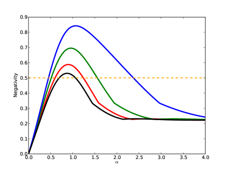
Figure 2: Negativity of the effective qutrit-qutrit state in dependence of $\alpha$ for various distances: 10 km (black), 8 km (red), 5 km (green) and 2 km (blue) (from bottom to top). The dashed, orange line indicates the negativity of a maximally entangled pure two-qubit Bell state.

The dashed orange line indicates the entanglement negativity of a pure maximally entangled qubit Bell state. Up to a distance of approximately $L_{0}=10\leavevmode\nobreak\ \text{km}$, it is possible to generate matter-qubus entanglement stronger than any, even ideal qubit-qubit entanglement. Taking into account that the realistic distribution of qubit-qubit entanglement is also subject to loss, the difference in entanglement negativity will be even more significant. However, a crucial step still is to transfer this entanglement to a sufficient extend from the matter-light system to a matter-matter system for storage.

III.4 Matter-matter qutrit-qutrit entanglement

To distribute entanglement between two matter qutrits, the light mode of the state in Eq.(28) interacts with a second matter system, initialized in the state $\frac{1}{\sqrt{3}}(|0\rangle+|1\rangle+|2\rangle)$. This time, similar to the qubit case, the controlled phase rotation takes place with the opposite angle, $\theta=-\frac{2\pi}{3}$. One obtains

$$\rho_{out} =\frac{N_{u}(\sqrt{1-\gamma}\alpha)}{9}|C_{0}\rangle\langle C_{0}|$$ (32)

$$+\frac{N_{v}(\sqrt{1-\gamma}\alpha)}{9}|C_{1}\rangle\langle C_{1}|$$

$$+\frac{N_{w}(\sqrt{1-\gamma}\alpha)}{9}|C_{2}\rangle\langle C_{2}|,$$

where the individual components are given by

$$|C_{0}\rangle =\frac{1}{\sqrt{3}}(|\phi_{00}\rangle|\sqrt{\gamma}\alpha\rangle$$ (33)

$$+|\phi_{02}\rangle|\sqrt{\gamma}\alpha e^{-\frac{2\pi i}{3}}\rangle+|\phi_{01}\rangle|\sqrt{\gamma}\alpha e^{\frac{2\pi i}{3}}\rangle),$$

$$|C_{1}\rangle =\frac{1}{\sqrt{3}}(|\phi_{20}\rangle|\sqrt{\gamma}\alpha\rangle+|\phi_{22}\rangle|\sqrt{\gamma}\alpha e^{-\frac{2\pi i}{3}}\rangle$$ (34)

$$+|\phi_{21}\rangle|\sqrt{\gamma}\alpha e^{\frac{2\pi i}{3}}\rangle),$$

$$|C_{2}\rangle =\frac{1}{\sqrt{3}}(|\phi_{10}\rangle|\sqrt{\gamma}\alpha\rangle+|\phi_{12}\rangle|\sqrt{\gamma}\alpha e^{-\frac{2\pi i}{3}}\rangle$$ (35)

$$+|\phi_{11}\rangle|\sqrt{\gamma}\alpha e^{\frac{2\pi i}{3}}\rangle),$$

with the two-qutrit Bell states from Eq.(22).

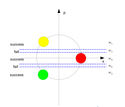
Figure 3: Phase space representation of the three coherent states $|\alpha\rangle$ and $|\alpha e^{\pm\frac{2\pi i}{3}}\rangle$ to be distinguished by USD.

In order to obtain entanglement between the two matter systems, the coherent states $|\sqrt{\gamma}\alpha\rangle,|\sqrt{\gamma}\alpha e^{-\frac{2\pi i}{3}}\rangle$, and $|\sqrt{\gamma}\alpha e^{\frac{2\pi i}{3}}\rangle$ have to be distinguished (see Fig. 3). Like in the loss-free case, this can be done using a homodyne measurement on the light mode. Unlike the qubit case, an $\hat{x}$-measurement is not suitable here, because $|\sqrt{\gamma}\alpha e^{\frac{2\pi i}{3}}\rangle$ and $|\sqrt{\gamma}\alpha e^{-\frac{2\pi i}{3}}\rangle$ cannot be distinguished. Therefore, we choose the quadrature $\hat{p}$ whose Gaussian momentum distribution for coherent states with complex amplitude $\beta$ reads as

$$|\psi_{\beta}(p)|^{2}=\sqrt{\frac{2}{\pi}}\exp\left(-2(p-\operatorname{Im}(\beta))^{2}\right).$$ (36)

This time, it is useful to define at least three windows to which a measurement result is assigned when the light mode of the output state in Eq.(32) is measured (see Fig.3). The first window is a symmetric interval around $p=0$, $w_{0}=[-\Delta,\Delta]$. A measurement result in this interval, similar to the qubit case, corresponds to an approximate projection on $|\alpha\rangle$. A projection onto the states $|\sqrt{\gamma}\alpha e^{\pm\frac{2\pi i}{3}}\rangle$ is assumed if a value falls into $w_{1}=[\frac{\sqrt{3}}{2}\sqrt{\gamma}\alpha-\Delta,\infty]$ or $w_{2}=[-\infty,-\frac{\sqrt{3}}{2}\sqrt{\gamma}\alpha+\Delta]$, respectively. Note that we need $\Delta\leq\frac{1}{2}\sqrt{\frac{3}{4}}\sqrt{\gamma}\alpha=:\Delta_{0}$ to exclude overlapping windows. We may decide to add two extra windows $w_{3}$ and $w_{4}$ to include the possibility of discarding measurement results (see Fig. 3). Inclusion of such failure events renders our qutrit entanglement distribution probabilistic.
Using the momentum wave functions for the coherent states, the qutrit-qutrit-qubus $|C_{0}\rangle$-component of $\rho_{out}$ after measuring the value $p$ in the homodyne detection of the qubus has the following conditional state for the two matter qutrits,

$$\sigma_{p}^{C_{0}} =\text{Tr}_{qubus}(|p\rangle\langle p|C_{0}\rangle\langle C_{0}|p\rangle\langle p|)$$ (37)

$$=\frac{1}{3}\bigg{(}|\phi_{00}\rangle\langle\phi_{00}|\cdot|\psi_{\sqrt{\gamma}\alpha}(p)|^{2}$$

$$+|\phi_{02}\rangle\langle\phi_{02}|\cdot|\psi_{\sqrt{\gamma}\alpha e^{-\frac{2\pi i}{3}}}(p)|^{2}$$

$$+|\phi_{01}\rangle\langle\phi_{01}|\cdot|\psi_{\sqrt{\gamma}\alpha e^{\frac{2\pi i}{3}}}(p)|^{2}$$

$$+|\phi_{00}\rangle\langle\phi_{02}|\cdot\psi_{\sqrt{\gamma}\alpha}(p)\psi^{*}_{\sqrt{\gamma}\alpha e^{-\frac{2\pi i}{3}}}(p)$$

$$+|\phi_{00}\rangle\langle\phi_{01}|\cdot\psi_{\sqrt{\gamma}\alpha}(p)\psi^{*}_{\sqrt{\gamma}\alpha e^{\frac{2\pi i}{3}}}(p)$$

$$+|\phi_{02}\rangle\langle\phi_{00}|\cdot\psi_{\sqrt{\gamma}\alpha e^{-\frac{2\pi i}{3}}}(p)\psi^{*}_{\sqrt{\gamma}\alpha}(p)$$

$$+|\phi_{02}\rangle\langle\phi_{01}|\cdot\psi_{\sqrt{\gamma}\alpha e^{-\frac{2\pi i}{3}}}(p)\psi^{*}_{\sqrt{\gamma}\alpha e^{\frac{2\pi i}{3}}}(p)$$

$$+|\phi_{01}\rangle\langle\phi_{00}|\cdot\psi_{\sqrt{\gamma}\alpha e^{\frac{2\pi i}{3}}}(p)\psi^{*}_{\sqrt{\gamma}\alpha}(p)$$

$$+\left.|\phi_{00}\rangle\langle\phi_{02}|\cdot\psi_{\sqrt{\gamma}\alpha e^{\frac{2\pi i}{3}}}(p)\psi^{*}_{\sqrt{\gamma}\alpha e^{-\frac{2\pi i}{3}}}(p)\right).$$

If we only accept the selection window $w_{0}=[-\Delta,\Delta]$, the resulting unnormalized state is obtained by doing the $p$-integration,

$$\sigma_{w_{0}}^{C_{0}}=\int\limits_{-\Delta}^{\Delta}dp\leavevmode\nobreak\ \sigma_{p}^{C_{0}}.$$ (38)

For carefully chosen $\Delta,\alpha$ and distance $L_{0}$, the contribution of the off-diagonal terms in Eq.(37) can be neglected such that we obtain the effective unnormalized state

$$\widetilde{\rho}_{w_{0}}^{C_{0}} =\frac{1}{3}\left(|\phi_{00}\rangle\langle\phi_{00}|\cdot\int\limits_{-\Delta}^{\Delta}dp\leavevmode\nobreak\ |\psi_{\sqrt{\gamma}\alpha}(p)|^{2}\right.$$ (39)

$$+|\phi_{02}\rangle\langle\phi_{02}|\cdot\int\limits_{-\Delta}^{\Delta}dp\leavevmode\nobreak\ |\psi_{\sqrt{\gamma}\alpha e^{-\frac{2\pi i}{3}}}(p)|^{2}$$

$$+\left.|\phi_{01}\rangle\langle\phi_{01}|\cdot\int\limits_{-\Delta}^{\Delta}dp\leavevmode\nobreak\ |\psi_{\sqrt{\gamma}\alpha e^{\frac{2\pi i}{3}}}(p)|^{2}\right).$$

The same calculation as above for $|C_{0}\rangle$ can be made for the other two components in $\rho_{out}$ of Eq. (32), $|C_{1}\rangle$ and $|C_{2}\rangle$. The total conditional (unnormalized) density matrix then becomes

$$\widetilde{\rho}_{w_{0}} =\frac{N_{u}(\sqrt{1-\gamma}\alpha)}{9}\widetilde{\rho}_{w_{0}}^{C_{0}}+\frac{N_{v}(\sqrt{1-\gamma}\alpha)}{9}\widetilde{\rho}_{w_{0}}^{C_{1}}$$ (40)

$$+\frac{N_{w}(\sqrt{1-\gamma}\alpha)}{9}\widetilde{\rho}_{w_{0}}^{C_{2}},$$

whose norm is the success probability,

$$p_{w_{0}} =\text{Tr}[\widetilde{\rho}_{w_{0}}]$$ (41)

$$=\frac{1}{3}\int\limits_{-\Delta}^{\Delta}dp\leavevmode\nobreak\ \left(|\psi_{\sqrt{\gamma}\alpha}(p)|^{2}+|\psi_{\sqrt{\gamma}\alpha e^{-\frac{2\pi i}{3}}}(p)|^{2}\right.$$

$$+\left.|\psi_{\sqrt{\gamma}\alpha e^{\frac{2\pi i}{3}}}(p)|^{2}\right),$$

where we used $\text{Tr}[\rho_{out}]=1$ and $\text{Tr}[\widetilde{\rho}_{w_{0}}^{C_{0}}]=\text{Tr}[\widetilde{\rho}_{w_{0}}^{C_{1}}]=\text{Tr}[\widetilde{\rho}_{w_{0}}^{C_{2}}]$. The corresponding fidelity for the target state is then calculated as

$$F_{w_{0}}=\frac{\langle\phi_{00}|\widetilde{\rho}_{w_{0}}|\phi_{00}\rangle}{p_{w_{0}}}$$ (42)

$$=\frac{N_{u}(\sqrt{1-\gamma}\alpha)}{9}\leavevmode\nobreak\ \frac{\frac{1}{3}\int\limits_{-\Delta}^{\Delta}dp\leavevmode\nobreak\ |\psi_{\sqrt{\gamma}\alpha}(p)|^{2}}{p_{w_{0}}}.$$

The success probabilities for the other two selection windows are obtained in complete analogy,

$$p_{w_{1}} =\frac{1}{3}\int\limits_{\frac{\sqrt{3}}{2}\sqrt{\gamma}\alpha-\Delta}^{\infty}dp\leavevmode\nobreak\ \left(|\psi_{\sqrt{\gamma}\alpha}(p)|^{2}+|\psi_{\sqrt{\gamma}\alpha e^{-\frac{2\pi i}{3}}}(p)|^{2}\right.$$ (43)

$$+\left.|\psi_{\sqrt{\gamma}\alpha e^{\frac{2\pi i}{3}}}(p)|^{2}\right),$$

$$p_{w_{2}} =\frac{1}{3}\int\limits_{-\infty}^{-\frac{\sqrt{3}}{2}\sqrt{\gamma}\alpha+\Delta}dp\leavevmode\nobreak\ \left(|\psi_{\sqrt{\gamma}\alpha}(p)|^{2}+|\psi_{\sqrt{\gamma}\alpha e^{-\frac{2\pi i}{3}}}(p)|^{2}\right.$$

$$+\left.|\psi_{\sqrt{\gamma}\alpha e^{\frac{2\pi i}{3}}}(p)|^{2}\right).$$

The corresponding fidelities with respect to the target states $|\phi_{01}\rangle$ and $|\phi_{02}\rangle$ for these windows are, respectively,

$$F_{w_{1}} =\frac{N_{v}(\sqrt{1-\gamma}\alpha)}{9}\leavevmode\nobreak\ \frac{\frac{1}{3}\int\limits_{\frac{\sqrt{3}}{2}\sqrt{\gamma}\alpha-\Delta}^{\infty}\leavevmode\nobreak\ |\psi_{\sqrt{\gamma}\alpha}(p)|^{2}}{p_{w_{1}}},$$ (44)

and

$$F_{w_{2}} =\frac{N_{w}(\sqrt{1-\gamma}\alpha)}{9}\leavevmode\nobreak\ \frac{\frac{1}{3}\int\limits_{-\infty}^{-\frac{\sqrt{3}}{2}\sqrt{\gamma}\alpha+\Delta}\leavevmode\nobreak\ |\psi_{\sqrt{\gamma}\alpha}(p)|^{2}}{p_{w_{2}}}.$$ (45)

To estimate the performance of this entanglement generation scheme, we define the average fidelity as

$$F_{av}=\frac{\sum\limits_{i=0}^{2}p_{w_{i}}F_{w_{i}}}{P_{succ}},$$ (46)

where $P_{succ}=\sum\limits_{i=0}^{2}p_{w_{i}}$ is the total success probability. The $\alpha$-dependence of the success probability and the average fidelity for various values of $\Delta$ is shown in Figs. 4 and 5 for $L_{0}$=5 km.
Clearly, if $\Delta=\Delta_{0}$, then there is no failure window at all and all measurement results are accepted. This corresponds to unit success probability, $P_{succ}=1$. On the other hand, for smaller (but not too small) $\Delta$, i.e., $\Delta<\Delta_{0}$, the success probability still tends to unity for increasing $\alpha$, as long as the three coherent states remain well within their respective selection windows. The fidelity, however, shows an opposite behavior. The smaller $\Delta$ is chosen, the higher the average fidelity for moderate values of $\alpha$. Increasing $\alpha$ makes the fidelity finally drop to 1/3, which is a direct consequence of the loss channel whose mixed output becomes more and more balanced for larger $\alpha$. For each chosen value of $\Delta$, there is an optimal value for $\alpha$ leading to a maximal fidelity. For instance, still with $L_{0}$=5 km, choosing $\Delta=0.2\Delta_{0}$ and $\alpha\approx 1$ leads to an average fidelity of $F_{av}\approx 0.7$ at a very reasonable success probability of $P_{succ}\approx 0.4$. The corresponding plots for elementary distances of $L_{0}$=10 km are shown in Figs. 6 and 7. A possible ququart scheme for distributing ququart-ququart entanglement is explicitly discussed in App. B.

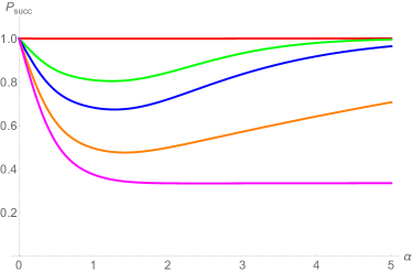
Figure 4: Success probability for the homodyne-based distribution of qutrit-qutrit entanglement over a distance of 5 km for various $\Delta$: $\Delta=\Delta_{0}$ (red), $\Delta=0.7\Delta_{0}$ (green), $\Delta=0.5\Delta_{0}$ (blue), $\Delta=0.2\Delta_{0}$ (orange) and $\Delta=0.001\Delta_{0}$ (magenta) (from top to bottom).

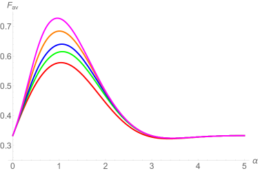
Figure 5: Average fidelity for the homodyne-based distribution of qutrit-qutrit entanglement over a distance of 5 km for various $\Delta$: $\Delta=\Delta_{0}$ (red), $\Delta=0.7\Delta_{0}$ (green), $\Delta=0.5\Delta_{0}$ (blue), $\Delta=0.2\Delta_{0}$ (orange) and $\Delta=0.001\Delta_{0}$ (magenta) (from bottom to top).

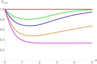
Figure 6: Success probability for the homodyne-based distribution of qutrit-qutrit entanglement over a distance of 10 km for various $\Delta$: $\Delta=\Delta_{0}$ (red), $\Delta=0.7\Delta_{0}$ (green), $\Delta=0.5\Delta_{0}$ (blue), $\Delta=0.2\Delta_{0}$ (orange) and $\Delta=0.001\Delta_{0}$ (magenta) (from top to bottom).

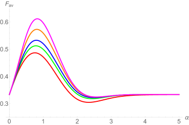
Figure 7: Average fidelity for the homodyne-based distribution of qutrit-qutrit entanglement over a distance of 10 km for various $\Delta$: $\Delta=\Delta_{0}$ (red), $\Delta=0.7\Delta_{0}$ (green), $\Delta=0.5\Delta_{0}$ (blue), $\Delta=0.2\Delta_{0}$ (orange) and $\Delta=0.001\Delta_{0}$ (magenta) (from bottom to top).

III.5 Unambiguous state discrimination

In this section, we will consider an alternative measurement scheme for a qutrit hybrid repeater based upon so-called unambiguous state discrimination (USD). Compared to the homodyne-based scheme, the conceptual difference in the USD-based scheme is that the non-orthogonality of the coherent states only affects $P_{succ}$ and no longer $F_{av}$, as USD enables one to discriminate non-orthogonal states probabilistically in an error-free fashion. The idea is that a successful and error-free projection onto one of the states $|\sqrt{\gamma}\alpha\rangle$ or $|\sqrt{\gamma}\alpha e^{\pm\frac{2\pi i}{3}}\rangle$ would lead to maximally entangled states in all components in Eq.(32). The task is therefore to find the most efficient possible scheme in the framework of quantum theory for unambiguously discriminating between the three coherent states above.
This problem was treated by Chefles Chefles who derived the optimal success probability as

$$P_{D}\leq\min\limits_{r}\sum\limits_{j=0}^{2}e^{-\frac{2\pi ijr}{3}}e^{\gamma\alpha^{2}(e^{\frac{2\pi ij}{3}}-1)},$$ (47)

with $r=0,1,2$ (see also Refs. vanEnk ; Croke ). The relation between this optimal probability and the corresponding fidelity of the final maximally entangled state is shown in Fig. 8.

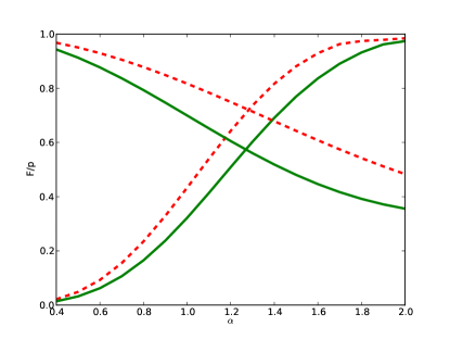
Figure 8: Success probabilities and fidelities for the USD-based scheme for 5 km (red, dotted) and 10 km (green, solid) in dependence of $\alpha$.

III.6 Entanglement purification

After the homodyne detection, the conditional state state resulting from Eq. (32) still represents a mixed state. Depending on the channel distance, the selection window, and the amplitude $\alpha$, the resulting state in the first component is a mixture of the dominant target state $|\phi_{00}\rangle$ with small extra components of $|\phi_{02}\rangle$ and $|\phi_{01}\rangle$ (if the result belongs to window $w_{0}$). This is similar for the other two components of the mixture with their rotated Bell states. Thus, effectively, the state after homodyne detection reads as (up to local qutrit rotations in case of the other two windows)

$$\rho_{eff} =\frac{N_{u}(\sqrt{1-\gamma}\alpha)}{9}|\widetilde{C}_{0}\rangle\langle\widetilde{C}_{0}|$$ (48)

$$+\frac{N_{v}(\sqrt{1-\gamma}\alpha)}{9}|\widetilde{C}_{1}\rangle\langle\widetilde{C}_{1}|$$

$$+\frac{N_{w}(\sqrt{1-\gamma}\alpha)}{9}|\widetilde{C}_{2}\rangle\langle\widetilde{C}_{2}|,$$

where

$$|\widetilde{C}_{0}\rangle =\frac{1}{\sqrt{3}}(|00\rangle+|11\rangle+|22\rangle),$$ (49)

$$|\widetilde{C}_{1}\rangle =\frac{1}{\sqrt{3}}(|00\rangle+e^{-\frac{2\pi i}{3}}|11\rangle+e^{\frac{2\pi i}{3}}|22\rangle),$$

$$|\widetilde{C}_{2}\rangle =\frac{1}{\sqrt{3}}(|00\rangle+e^{+\frac{2\pi i}{3}}|11\rangle+e^{-\frac{2\pi i}{3}}|22\rangle).$$

Note that in the case of USD, Eqs. (48) and (49) represents the exact output state and there are no extra terms from the rotated Bell states (which nonetheless can be neglected for the case of homodyne detection provided the selection window-based state discrimination works sufficiently well). In general, mixed entangled states degrade the performance of quantum information processing tasks like teleportation or the entanglement swapping operation discussed in the next section. Hence, a purification of the above mixed state is required.
Entanglement purification aims at generating fewer high-fidelity copies from many noisy copies of a certain pure target state via local operations and classical communication. By iterating this purification protocol, a fidelity arbitrarily close to unity can be achieved. The purification of mixed qubit states was investigated by Bennett et. al Bennett for the class of Werner states Werner2 . Nearly at the same time, Deutsch et al. Deutsch demonstrated a similar purification protocol for states diagonal in the Bell basis. This protocol requires only two copies for each step and leads to a better efficiency compared to the Bennett scheme. The latter was demonstrated experimentally Pan2001 ; Pan2003 and also generalized to arbitrary dimensions Horodecki ; Alber .
To perform a purification of our relevant state, i.e. to increase the statistical weight of $|\widetilde{C}_{0}\rangle$ in Eq. (48), at least two copies of the matter-matter output state are required. On each copy, the following transformations are performed: The first matter qutrit system is subject to the transformation

$$|0\rangle \mapsto\frac{1}{\sqrt{3}}(|0\rangle+|1\rangle+|2\rangle),$$ (50)

$$|1\rangle \mapsto\frac{1}{\sqrt{3}}(|0\rangle+e^{i\phi}|1\rangle+e^{-i\phi}|2\rangle),$$

$$|2\rangle \mapsto\frac{1}{\sqrt{3}}(|0\rangle+e^{-i\phi}|1\rangle+e^{i\phi}|2\rangle),$$

while on the second system,

$$|0\rangle \mapsto\frac{1}{\sqrt{3}}(|0\rangle+|1\rangle+|2\rangle),$$ (51)

$$|1\rangle \mapsto\frac{1}{\sqrt{3}}(|0\rangle+e^{-i\phi}|1\rangle+e^{i\phi}|2\rangle),$$

$$|2\rangle \mapsto\frac{1}{\sqrt{3}}(|0\rangle+e^{i\phi}|1\rangle+e^{-i\phi}|2\rangle),$$

is performed where $\phi=\frac{2\pi}{3}$. The components of the mixture are then transformed as

$$|\widetilde{C}_{0}\rangle \mapsto\frac{1}{\sqrt{3}}(|00\rangle+|11\rangle+|22\rangle),$$ (52)

$$|\widetilde{C}_{1}\rangle \mapsto\frac{1}{\sqrt{3}}(|01\rangle+|12\rangle+|20\rangle),$$

$$|\widetilde{C}_{2}\rangle \mapsto\frac{1}{\sqrt{3}}(|10\rangle+|21\rangle+|02\rangle).$$

A mixture of $|\widetilde{C}_{0}\rangle$, $|\widetilde{C}_{1}\rangle$, and $|\widetilde{C}_{2}\rangle$ with statistical weights $p_{0}$, $p_{1}$, and $p_{2}$, where $p_{0}+p_{1}+p_{2}=1$, can now be purified as follows. One takes two copies of the state that is shared between two parties $A$ and $B$. As proven in Sec. IV for arbitrary dimensions, local subtraction gates are applied on the qutrits belonging to A and B. After this, A and B select one of the two copies and measure its respective spin. Equal spin results lead to the new mixed state

$$\rho^{\prime}=\frac{\sum\limits_{j=0}^{2}p_{j}^{2}|\widetilde{C}_{j}\rangle\langle\widetilde{C}_{j}|}{\sum\limits_{j=0}^{2}p_{j}^{2}},$$ (53)

whose fidelity with respect to the target state $|\widetilde{C_{0}}\rangle$ is now increased, provided $p_{0}>1/3$ and $p_{1},p_{2}<p_{0}$.

III.7 Entanglement swapping

In the previous sections, we have shown how to entangle two qutrits over a distance $L_{0}$. The distance $L_{0}$, however, is typically to short for general applications in quantum communication. It is therefore necessary to further extend the entanglement over larger distances. This can be done by entanglement swapping.
To perform entanglement swapping, two entangled qutrit-qutrit pairs are generated next to each other, covering a total distance of $2L_{0}$. To connect the two pairs and thus distribute entanglement over twice the initial distance, a Bell measurement is carried out on the two adjacent matter systems. A successful Bell measurement projects the remaining two matter systems onto a maximally entangled state.
In analogy to the qubit case, a Bell measurement on two qutrits can be performed by applying a qudit sum gate (cnot or cshift), followed by measurements in the $X$ and in the $Z$ basis (see Eq. (18)). As pointed out in Dusek , Hadamard transformations and a cphase gate suffice to implement the sum gate.
In the following, we assume that arbitrary single qutrit rotations and measurements can be performed on the matter systems and show how to construct the sum gate based on these assumptions.
In our framework, a cphase gate is represented by the unitary operation

$$U_{CP}=\exp\left(-\frac{2\pi i}{3}S_{z_{1}}^{(3)}S_{z_{2}}^{(3)}\right),$$ (54)

where the operators $S_{z_{i}}^{(3)}$ correspond to the operations introduced in Eq.(18) on the ith qutrit. Like in the qubit case of a cnot gate, a decomposition for the qudit cshift gate is given by

$$\operatorname{\textsc{cshift}}=(H\otimes\mathbbm{1})\cdot\operatorname{\textsc{cphase}}\cdot(H\otimes\mathbbm{1}),$$ (55)

where $H$ is the qutrit Hadamard transformation. Indeed, one observes by direct calculation $(H\otimes\mathbbm{1})\operatorname{\textsc{cphase}}(H\otimes\mathbbm{1})|x,y\rangle=|x\ominus y,y\rangle$ for $x,y\in\mathbb{Z}_{2}$. Note that $\ominus$ denotes subtraction modulo 3. A more formal proof of this decomposition for arbitrary dimensions is given in Sec. IV.
With HQR protocols for qubits and qutrits in mind, an extension to ququarts, i.e. four-level systems, is straightforward. As a bridge to the general qudit case, as presented in the next section, it is nonetheless useful to also explicitly consider the ququart case including the optical qubus measurements adapted to this case. It is presented in App. A.

III.8 Rate analysis

III.8.1 Methods and assumptions

In this section, we quantify the performance of our qutrit HQR protocol for the generation of entanglement over the total channel distance $L_{0}$. The performance can be assessed by the entanglement generation rate, i.e., the number of entangled pairs over the entire distance per unit time. Besides this, the fidelity of the generated states is of particular interest.
The atomic matter systems also serve as quantum memories (as needed because of the probabilistic step of entanglement purification after the entanglement distribution) and we assume matter systems with infinite coherence time, i.e. perfect memories. In addition, we assume deterministic and error-free gates on them. Especially, the entanglement swapping operation is treated as deterministic employing the gates as described in the preceeding section. Strictly speaking, photon transmission loss is the only error source entering our rate analysis and the resulting rates have to be understood as upper bounds of the actual achievable rates. For this scenario, analytical formulae for the rates in dependence of the number of elementary segments as well as the number of purifications performed on each segment after the distributions have been derived in rate . Note that we include one to several rounds of entanglement purification only right after the initial entangled-state distributions. In this theoretical treatment, our repeater scheme effectively becomes a second generation quantum repeater (recall Sec. I) where rates are ultimately limited by $R\lesssim\frac{c}{L_{0}}$ (instead of $R\lesssim\frac{c}{L}$ if purifications were performed until the final nesting level Briegel1 ; Briegel2 ) Ultrafast ; Optiarchi .
We consider $2^{n}$ segments of elementary distance $L_{0}$, covering a total distance $L=2^{n}L_{0}$. Entanglement is generated in each segment with a probability $P_{0}$. If the obtained state is not directly purified, the resulting rate becomes

$$R_{n}=\frac{c}{2L_{0}}\frac{1}{Z_{n}(P_{0})}=\frac{1}{T_{0}Z_{n}(P_{0})}$$ (56)

where

$$Z_{n}(P_{0})=\sum\limits_{j=1}^{2^{n}}\binom{2^{n}}{j}\frac{1}{1-(1-P_{0})^{j}}$$ (57)

is the average total number of attempts it takes for all segments to eventually share an entangled pair (recall that initially shared pairs can be stored as long as needed), $T_{0}=\frac{2L_{0}}{c}$ is the elementary time unit for sending the quantum states and also the classical information to confirm their successful distribution (as well as purification), and $c$ is the speed of light in the optical fiber.
If one round of purification is performed, the same formula can be applied, but now $P_{0}$ has to be substituted by an effective probability,

$$Q_{1}(L_{0})=P_{0}P_{1}\left(\frac{2-P_{0}}{3-2P_{0}}\right),$$ (58)

where $P_{1}$ is the probability for the first round of purification to succeed. Furthermore, the rates with two and three rounds of purification can be calculated using the effective probabilities

$$Q_{2}(L_{0})=Q_{1}(L_{0})P_{2}\left(\frac{2-Q_{1}(L_{0})}{3-2Q_{1}(L_{0})}\right),$$ (59)

and

$$Q_{3}(L_{0})=Q_{2}(L_{0})P_{3}\left(\frac{2-Q_{2}(L_{0})}{3-2Q_{2}(L_{0})}\right),$$ (60)

where $P_{2}$ and $P_{3}$ are the success probabilities for two and three rounds of purification, respectively. Note that without the use of quantum memories, $Q_{3}$ would scale as $P_{0}^{8}P_{1}^{4}P_{2}^{2}P_{3}$, which (assuming small probabilities) is turned into a scaling like $P_{0}P_{1}P_{2}P_{3}$ with the help of the quantum memories. Higher rounds of purification can be considered in a recursive fashion. We analyze the rates for the USD- and homodyne-based scheme separately in the next two sections.

III.8.2 USD-based scheme

For the USD-scheme, $P_{0}$ is given by the optimal probability in Eq.(47) to distinguish the three coherent states $|\sqrt{\gamma}\alpha\rangle$ and $|\sqrt{\gamma}\alpha e^{\frac{2\pi i}{3}}\rangle$. The resulting state is the normalized version of Eq. (39) and the initial fidelity of the target state reads as

$$F_{0}=\frac{N_{u}(\sqrt{1-\gamma}\alpha)}{9},$$ (61)

and

$$F_{1} =\frac{N_{v}(\sqrt{1-\gamma}\alpha)}{9},$$ (62)

$$F_{2} =\frac{N_{w}(\sqrt{1-\gamma}\alpha)}{9},$$

for the other two components. One round of purification succeeds with probability

$$P_{1}=F_{0}^{2}+F_{1}^{2}+F_{2}^{2},$$ (63)

and the resulting improved fidelity is

$$F_{0}^{\prime}=\frac{F_{0}^{2}}{F_{0}^{2}+F_{1}^{2}+F_{2}^{2}}.$$ (64)

For more rounds of purification, the fidelities and success probabilities can be obtained recursively.
After entanglement swapping, the final fidelity of the entangled state distributed over the total distance is lower bounded by $(\widetilde{F}_{0})^{2^{n}}$, where $\widetilde{F}_{0}$ is the final fidelity for each segment, possibly obtained after some rounds of purification.

III.8.3 Homodyne-based scheme

An exact rate analysis for the HQR with entanglement distribution based on homodyne detection is much more demanding than for the USD-case. This is due to the fact that at adjacent elementary segment potentially different mixed quantum states are generated depending on the corresponding measurement result. As already pointed out, these states can be brought into a similar form, i.e., the components are equal, but the statistical weights are not necessarily equal. An exact rate analysis is therefore out of reach.
To nevertheless assess the performance of that scheme, we model the situation with an effective state on each elementary segment. This effective state has the average fidelity $F_{av}(\alpha,\gamma)$ as the statistical weight of the first component, whereas the other two components are equally weighted with $F_{1}=F_{2}=\frac{1}{2}(1-F_{av}(\alpha,\gamma))$. For an elementary distance of $L_{0}=5$ km, we choose $\alpha\approx 1$, which leads to a maximum initial fidelity of $\approx 0.7$. As the generation probability $P_{0}$, we insert the success probability, $P_{succ}=\sum\limits_{i=0}^{2}p_{w_{i}}$, for obtaining a result in one of the success windows (see Sec. III.4) which equals $\approx 0.4$ in this case. For $L_{0}=10$ km, we also have $\alpha\approx 1$, but now $F_{av}\approx 0.6$ and $P_{0}\approx 0.39$.
Using these initial values, the formulae for the rates and fidelities, including some possible rounds of purification, can directly be applied. For quantitative examples and an illustration of the trade-off between repeater rates and fidelities, see App. A.
To summarize some of the results presented there, for elementary distances as short as $L_{0}=5$ km, the USD-based scheme and the homodyne-based scheme perform comparably. In either case at least three rounds of purification are needed in order to obtain reasonable fidelities and rates for distances as large as 640 km. For $L_{0}=10$ km according to our calculations, the USD-based scheme performs slightly better than the homodyne-based scheme, such that in both scenarios rather high fidelities can be achieved for distances as large as 1280 km (the rates are comparable and again three rounds of purification are necessary). However, note that our results for the homodyne-based scheme only hold under the assumptions that the off-diagonal terms in Eq.(37) are negligible and that the conditional state after homodyne detection can be modeled via an effective state with fidelity $F_{av}$. Thus, the numbers presented in App. A may overestimate the homodyne-based scheme compared to the USD-based scheme.
Results for a situation with a more practical repeater spacing, $L_{0}=20$ km, indicate that for $L=1280$ km near-unit fidelities at rates $\sim$ Hz are only achievable using USD, because in the homodyne-based scheme the output fidelities drop below 0.5 for such large elementary distances. Note that a similar observation was made for the original qubit scheme based on homodyne detection Bright .

IV The general qudit case

Based on the results obtained in the last sections for specific examples, we are now in turn to propose HQR protocols for arbitrary finite dimensional quantum systems.
The dispersive interaction between a general qudit, i.e. a $d$-level system, and a light mode can be realized by the Hamiltonian

$$H_{int}^{(d)}=\hbar gS_{z}^{(d)}a^{\dagger}a$$ (65)

with $S_{z}^{(d)}|k\rangle=\left(\frac{2k-d+1}{2}\right)|k\rangle$ for $k=\{0,1,..,d-1\}$, and where $S_{z}^{(2)}=\sigma_{z}$. The corresponding unitary is $U_{d}(\theta)=\exp(i\theta S_{z}^{(d)}a^{\dagger}a)$ and the relevant case of a strong interaction is obtained by setting $\theta=\frac{2\pi}{d}$.
The first step in the protocol is the preparation of the matter state $\frac{1}{\sqrt{d}}\sum\limits_{k=0}^{d-1}|k\rangle$, which then interacts with an optical coherent state $|\alpha\rangle$ via the strong dispersive interaction. This results in a hybrid entangled qudit-light (qudit-qubus) state,

$$\frac{1}{\sqrt{d}}\sum\limits_{k=0}^{d-1}|k\rangle|\alpha e^{\frac{2k\pi ik}{d}}\rangle.$$ (66)

After locally generating qudit-light entanglement, the light mode is sent through an optical channel of length $L_{0}$ where it is subject to photon loss. Including again an ancilla vacuum mode and mixing it with the optical mode results in

$$\frac{1}{\sqrt{d}}\sum\limits_{q=0}^{d-1}|q\rangle|\sqrt{\gamma}\alpha e^{\frac{2\pi iq}{d}}\rangle|\sqrt{1-\gamma}\alpha e^{\frac{2\pi iq}{d}}\rangle.$$ (67)

As in the specific examples above, the crucial point is now to find a suitable basis for tracing out the loss mode. Here, in the general case, this basis consists of the $d$ vectors

$$|v_{m}\rangle=\frac{1}{\sqrt{N_{v_{m}}(\alpha)}}\sum\limits_{k=0}^{d-1}e^{\frac{2\pi ikm}{d}}|\alpha e^{\frac{2\pi ik}{d}}\rangle,$$ (68)

with $m=0,1,..,d-1$. We can thus recast the coherent states of the ancilla light mode in Eq. (67) as

$$|\alpha e^{\frac{2\pi ik}{d}}\rangle=\frac{1}{d}\sum\limits_{m=0}^{d-1}\sqrt{N_{v_{m}}(\alpha)}e^{-\frac{2\pi ikm}{d}}|v_{m}\rangle,$$ (69)

and find for Eq. (67):

$$\frac{1}{d\sqrt{d}}\sum\limits_{q,m=0}^{d-1}\sqrt{N_{v_{m}}(\sqrt{1-\gamma}\alpha)}e^{-\frac{2\pi iqm}{d}}|q\rangle|\sqrt{\gamma}\alpha e^{\frac{2\pi iq}{d}}\rangle|v_{m}\rangle.$$ (70)

Tracing out the loss mode in this basis is now a trivial task and one obtains

$$\rho_{out} =\sum\limits_{m=0}^{d-1}\frac{N_{v_{m}}(\sqrt{1-\gamma}\alpha)}{d^{2}}$$ (71)

$$\times\left[\left(\frac{1}{\sqrt{d}}\sum\limits_{q=0}^{d-1}e^{-\frac{2\pi iqm}{d}}|q\rangle|\sqrt{\gamma}\alpha e^{\frac{2\pi iq}{d}}\rangle\right)\times H.c.\right]$$

for the $d$-component qudit-light output state.
Again, this can be further simplified by basis transformations on both the light mode and the matter system. The light mode can be expressed in the basis given in Eq. (68), while the matter system can be written in the (generalized Pauli) qudit X-basis,

$$|\widetilde{k}\rangle=\frac{1}{\sqrt{d}}\sum\limits_{m=0}^{d-1}e^{\frac{2\pi ikm}{d}}|m\rangle,$$ (72)

for $k=0,1,...,d-1$. This gives the expression

$$\rho_{out} =\sum\limits_{m=0}^{d-1}\frac{N_{v_{m}}(\sqrt{1-\gamma}\alpha)}{d^{2}}$$ (73)

$$\times \left[\left(\frac{1}{d}\sum\limits_{r=0}^{d-1}\sqrt{N_{v_{r}}}|\widetilde{m\oplus r}\rangle|\widetilde{v}_{r}\rangle\right)\times H.c.\right]$$

for Eq. (71) where $\oplus$ denotes addition modulo $d$. Note that $\sim$ again indicates basis vectors with damped amplitude $\sqrt{\gamma}\alpha$ on the light mode and the X-basis on the matter system.
After traveling through the loss channel over a distance $L_{0}$, the light mode reaches a second matter system, also prepared in the state $\frac{1}{\sqrt{d}}\sum\limits_{k=0}^{d-1}|k\rangle$. The light mode interacts dispersively with the second matter system, this time with the inverse angle $\theta=-\frac{2\pi}{d}$. The resulting state becomes

$$\rho=\sum\limits_{m=0}^{d-1}\frac{N_{v_{m}}}{d^{2}}|T_{m}\rangle\langle T_{m}|,$$ (74)

with the components

$$|T_{m}\rangle=\frac{1}{d}\sum\limits_{q=0}^{d-1}\sum\limits_{l=0}^{d-1}e^{-\frac{2\pi iqm}{d}}|q\rangle|l\rangle|\sqrt{\gamma}\alpha e^{\frac{2\pi i(q-l)}{d}}\rangle,$$ (75)

written in the original basis (like in Eq.(71)).
The state discrimination in the general case involves the $d$ coherent states $|\sqrt{\gamma}\alpha\rangle,...,|\sqrt{\gamma}\alpha e^{\frac{2\pi i(d-1)}{d}}\rangle$ which can be graphically represented as coherent states "on a ring" (see Fig. 9  for $d=8$). A projection onto one of the $d$ coherent states collapses each component onto a maximally entangled state. However, by increasing the dimension $d$, a projection scheme based on homodyne detection becomes more and more futile since no direction is uniquely specified any more.

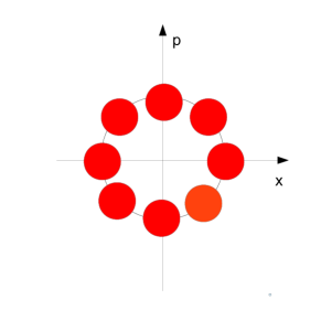
Figure 9: Phase space representation of the qubus mode for $d=8$.

A scheme for unambiguously discriminating exactly these $d$ coherent states was derived in Chefles for arbitrary dimensions (for $d=3$, recall Sec. III.5). An upper bound for the success probability is given by

$$P_{D}\leq\min\limits_{r}\sum\limits_{j=0}^{d-1}e^{-\frac{2\pi ijr}{d}}e^{\gamma\alpha^{2}(e^{\frac{2\pi ij}{d}}-1)},$$ (76)

$r=0,1,..,d-1$, where Eq.(47) is recovered for $d=3$. Since the upper bound on the right-hand side depends on both $\alpha$ and $\gamma$ the minimization with respect to $r$ is hard analytically. We therefore calculate the bound numerically.
After the USD, the resulting mixed state will be a mixture of $d-1$ maximally entangled Bell states of the form

$$|\phi_{kj}\rangle=\frac{1}{\sqrt{d}}\sum\limits_{y=0}^{d-1}e^{\frac{2\pi iky}{d}}|y,y\ominus j\rangle,$$ (77)

for one fixed $j=0,...,d-1$, according to the specific identified coherent state.
If $j\neq 0$, a $j$-fold application of $X=\sum\limits_{k=0}^{d-1}|k+1\rangle\langle k|$ transforms all these states to

$$|\phi_{k0}\rangle=\frac{1}{\sqrt{d}}\sum\limits_{y=0}^{d-1}e^{\frac{2\pi iky}{d}}|y,y\rangle.$$ (78)

By means of local unitaries, the different components of the mixtures with $|\phi_{k0}\rangle$ can always be transformed to a mixture of the states

$$|\psi_{j}\rangle\equiv|\phi_{0j}\rangle=\frac{1}{\sqrt{d}}\sum\limits_{y=0}^{d-1}|y,y\ominus j\rangle,$$ (79)

with now all $j$ included. We therefore obtain

$$\rho=\sum\limits_{j=0}^{d-1}p_{j}|\psi_{j}\rangle\langle\psi_{j}|$$ (80)

for the state to be purified.
The purification now works as follows. We prepare two copies of the state in Eq.(80) such that the total joint four-qudit state reads

$$\rho\otimes\rho=\sum\limits_{j=0}^{d-1}\sum\limits_{k=0}^{d-1}p_{j}p_{k}|\psi_{j}\rangle|\psi_{k}\rangle\langle\psi_{j}|\langle\psi_{k}|,$$ (81)

where the individual terms are

$$|\psi_{j}\rangle|\psi_{k}\rangle=\frac{1}{d}\sum\limits_{y=0}^{d-1}\sum\limits_{y^{\prime}=0}^{d-1}|y,y\ominus j\rangle|y^{\prime},y^{\prime}\ominus k\rangle.$$ (82)

One applies a local CSHIFT gate on systems 1 and 3 as well 2 and 4 in order to obtain

$$\frac{1}{d}\sum\limits_{y=0}^{d-1}\sum\limits_{y^{\prime}=0}^{d-1}|y-y^{\prime},y\ominus y^{\prime}\oplus k\ominus j\rangle|y^{\prime},y^{\prime}\ominus k\rangle.$$ (83)

After that, the first spins of the first two systems are measured. If the spins are parallel, it follows $k=j$ such that only diagonal parts contribute. As a consequence, the second two systems collapse to $|\psi_{k}\rangle$.
The new state then becomes

$$\rho^{\prime}=\frac{\sum\limits_{j=0}^{d-1}p_{j}^{2}|\psi_{j}\rangle\langle\psi_{j}|}{\sum\limits_{j=0}^{d-1}p_{j}^{2}}.$$ (84)

The fidelity with respect to the target state $|\psi_{0}\rangle$ is thus

$$F^{\prime}=\frac{p_{0}^{2}}{\sum\limits_{j=0}^{d-1}p_{j}^{2}},$$ (85)

which is increased compared to the initial fidelity $p_{0}$ if $p_{0}>\frac{1}{d}$ and $p_{i}<p_{0}$ for $i=1,...,d-1$.
After possibly several rounds of purification, a high-fidelity entangled state can be obtained between the two separated qudits. This is referred to as the initial entanglement generation or distribution.
To further extend the entanglement, two elementary segments next to each other are connected via entanglement swapping through Bell measurements on adjacent repeater nodes, i.e., a projection on maximally entangled qudit-qudit states.
Generalizing the qutrit case, we show that the cshift gate lies at the heart of such Bell measurements and that these be realized by a cphase gate based on the generalized dispersive interaction.
The cphase gate for an arbitrary dimension $d$ is realized by the two-qudit unitary transformation

$$U_{d}=\exp\left(-\frac{2\pi i}{d}S_{z_{1}}^{(d)}S_{z_{2}}^{(d)}\right),$$ (86)

with the generalized spin operator $S_{i}^{(d)}$ acting on qudit $i$. We show by direct calculation that the sequence $H\otimes 1\rightarrow\textsc{cphase}\rightarrow H\otimes 1$ acts as a controlled phase shift gate on an arbitrary two-qudit state:

$$(H\otimes 1)\cdot\textsc{cphase}\cdot(H\otimes 1)|xy\rangle$$ (87)

$$=(H\otimes 1)\cdot\textsc{cphase}\frac{1}{\sqrt{d}}\sum\limits_{k=0}^{d-1}\exp\left(\frac{2\pi ikx}{d}\right)|ky\rangle$$

$$=(H\otimes 1)\frac{1}{\sqrt{d}}\sum\limits_{k=0}^{d-1}\exp\left(\frac{2\pi ik(x-y)}{d}\right)|ky\rangle$$

$$=|x-y,y\rangle.$$

Together with arbitrary qudit rotations and measurements in the qudit $X$ and $Z$ basis, this suffices to implement a deterministic Bell state analyzer for qudits Dusek .

V Discussion and Conclusions

We introduced a hybrid quantum repeater protocol for the distribution of arbitrary finite-dimensional bipartite entangled states over large distances with a specific focus on qutrit entanglement. A generalization of the dispersive light-matter interaction from the qubit to the general qudit case lies at the heart of our protocol and can be expressed by higher spin operators. The distribution of matter-matter entanglement between neighboring repeater stations is mediated via coherent states interacting dispersively and subsequently with the matter systems. We investigated both USD and homodyne detection of the light mode and compared the rates and final fidelities. By exploiting purification on the elementary segments, sufficiently high initial fidelities can be achieved to cover distances up to 1280 km with final fidelities close to unity. With three rounds of entanglement purification directly after the initial entanglement distributions, rates $\sim$ 100 Hz are, in principle, possible.
Since our scheme assumes perfect matter systems (with perfect coherence properties for arbitrarily long times) and operations on them, future research may aim at investigating different physical platforms and decoherence models for the matter systems. Like for the qubit case hybridencoding , quantum error correction codes could be employed on the matter systems turning the scheme to a genuine second generation quantum repeater scheme and thus preserving the communication rates obtained here under idealizing assumptions.

VI Acknowledgement

We acknowledge support from Q.com (BMBF).

Appendix A Rate analysis for qutrit hybrid quantum repeater

In this appendix, we show several tables summarizing the results on the rates and fidelities for our qutrit quantum repeater scheme ($d=3$), as described in Sec. III.8. We consider various total distances up to 1280 km, two possible elementary distances ($L_{0}=5,10$ km), between zero and three rounds of entanglement purification directly after the initial entanglement distribution, and the two possible detection schemes (homodyne, USD).

	rounds of purification	no	one	two	three
	initial fidelity	0.75	0.94393	0.997854	0.999996
	effective probability	0.64	0.302641	0.19154	0.1318
rate [Hz]	10 km	10175	4290	2647	900
	20 km	7936	3185	1942	656
	40 km	6366	2488	1506	507
	80 km	5285	2024	1220	409
	160 km	4501	1701	1021	342
	320 km	3914	1464	877	294
	640 km	3461	1284	768	257
fidelity	10 km	0.56	0.891	0.9957	0.99999265
	20 km	0.315	0.793	0.9914	0.999998531
	40 km	0.09	0.63	0.983	0.99997061
	80 km	0	0.397	0.966	0.99994123
	160 km	0	0.158	0.934	0.99988246
	320 km	0	0.02	0.872	0.99976494
	640 km	0	0	0.761	0.99952994

Table 1: $L_{0}$=5 km (USD), $\alpha=1.2$, $L\leq$ 640 km

	rounds of purification	no	one	two	three
	initial fidelity	0.652	0.87	0.987	0.999
	effective probability	0.414	0.147	0.078	0.05
rate [Hz]	20 km	3020	1010	524	343
	40 km	2271	738	380	248
	80 km	1788	570	293	191
	160 km	1463	461	236	156
	320 km	1234	385	197	128
	640 km	1065	331	169	110
	1280 km	936	289	147	96
fidelity	20 km	0.420	0.76	0.974	0.999
	40 km	0.18	0.57	0.95	0.999
	80 km	0.03	0.33	0.9	0,999
	160 km	0.001	0.1	0.814	0.998
	320 km	0	0.01	0.66	0.996
	640 km	0	0	0.436	0.992
	1280 km	0	0	0.19	0.984

Table 2: $L_{0}$=10 km (USD), $\alpha=1.2$, $L\leq$ 1280 km

	rounds of purification	no	one	two	three
	initial fidelity	0.73	0.93	0.997	0.999997
	effective probability	0.38	0.15	0.09	0.0619534
rate [Hz]	10 km	5496	2056	1219	835
	20 km	4117	1502	885	605
	40 km	3233	1161	682	465
	80 km	2641	939	550	375
	160 km	2225	785	459	313
	320 km	1919	674	394	267
	640 km	1686	589	344	234
fidelity	10 km	0.53	0.86	0.995	0.999994
	20 km	0.28	0.75	0.990	0.999987
	40 km	0.08	0.56	0.980	0.999975
	80 km	0.01	0.31	0.961	0.99995
	160 km	0.00	0.10	0.923	0.9999
	320 km	0.00	0.01	0.852	0.9998
	640 km	0.00	0.00	0.726	0.9996

Table 3: $L_{0}$=5 km (homodyne), $\alpha\approx 1$, $L\leq$ 640 km

	rounds of purification	no	one	two	three
	initial fidelity	0.6	0.81	0.974	0.9996
	effective probability	0.39	0.12	0.057	0.037
rate [Hz]	20 km	2828	817	384	246
	40 km	2121	595	278	178
	80 km	1667	460	214	137
	160 km	1362	371	172	110
	320 km	1148	310	144	92
	640 km	990	266	123	79
	1280 km	870	233	107	69
fidelity	20 km	0.360	0.656	0.949	0.999
	40 km	0.130	0.430	0.900	0.999
	80 km	0.017	0.185	0.810	0.997
	160 km	0.000	0.034	0.656	0.994
	320 km	0.000	0.001	0.430	0.989
	640 km	0	0	0.184	0.978
	1280 km	0	0	0.03	0.957

Table 4: $L_{0}$=10 km (homodyne), $\alpha\approx 1$, $L\leq$ 1280 km

	rounds of purification	no	one	two
	initial fidelity	0.861808	0.986275	0.999876
	effective probability	0.0137597	0.0069238	0.0044958
rate [Hz]	40 km	92	46	30
	80 km	33	17	11
	160 km	26	13	9
	320 km	21	11	7
	640 km	17	9	6
	1280 km	15	8	5
fidelity	20 km	0.360	0.656	0.949
	40 km	0.130	0.973	0.9997
	80 km	0.017	0.946	0.9995
	160 km	0.000	0.895	0.9990
	320 km	0.09	0.802	0.9980
	640 km	0	0	0.9960
	1280 km	0	0	0.9921

Table 5: $L_{0}$=20 km (USD), $\alpha=0.5$, $L\leq$ 1280 km

Appendix B Ququart hybrid repeater

The dispersive interaction acting on a ququart-light system is defined by the unitary transformation

$$U_{4}(\theta) \left[\frac{1}{2}(|0\rangle+|1\rangle+|2\rangle+|3\rangle)|\alpha\rangle\right]=\frac{1}{2}(|0\rangle|\alpha\rangle+|1\rangle|\alpha e^{i\theta}\rangle+|2\rangle|\alpha e^{2i\theta}\rangle+|3\rangle|\alpha e^{3i\theta}\rangle),$$ (88)

which is induced by the Hamiltonian $H_{int}^{(4)}=\hbar gS^{(4)}_{z}a^{\dagger}a$ with $S^{(4)}_{z}|k\rangle=\left(\frac{2k-3}{2}\right)|k\rangle$ for $k\in\{0,1,2,3\}$. Thus, the ququart (4-level system) may be represented by a spin-$\frac{3}{2}$ particle. The case of a strong interaction is obtained by choosing $\theta=\frac{\pi}{2}$.
As before, the first step in the protocol is the generation of an entangled ququart-light state via the strong dispersive interaction, i.e.,

$$\frac{1}{2}(|0\rangle|\alpha\rangle+|1\rangle|i\alpha\rangle+|2\rangle|-\alpha\rangle+|3\rangle|-i\alpha\rangle),$$ (89)

of which the light part is then sent through the optical channel over a distance $L_{0}$, suffering from loss.
The output density matrix is again determined by mixing the light mode with an ancilla vacuum state and tracing out the light mode. It is again useful to transform the coherent states of the light field into an orthogonal basis. The adapted orthogonal basis in this case reads

$$|u\rangle =\frac{1}{\sqrt{N_{u}(\alpha)}}(|\alpha\rangle+|-\alpha\rangle+|i\alpha\rangle+|-i\alpha\rangle),$$ (90)

$$|v\rangle =\frac{1}{\sqrt{N_{v}(\alpha)}}(|\alpha\rangle+i|-\alpha\rangle-|i\alpha\rangle-i|-i\alpha\rangle),$$

$$|w\rangle =\frac{1}{\sqrt{N_{w}(\alpha)}}(|\alpha\rangle-|-\alpha\rangle+|i\alpha\rangle-|-i\alpha\rangle),$$

$$|z\rangle =\frac{1}{\sqrt{N_{z}(\alpha)}}(|\alpha\rangle-i|-\alpha\rangle-|i\alpha\rangle+i|-i\alpha\rangle),$$

with normalization constants $N_{u}(\alpha),N_{v}(\alpha),N_{w}(\alpha),$ and $N_{z}(\alpha)$. We can therefore write

$$|\alpha\rangle =\frac{1}{4}(\sqrt{N_{u}(\alpha)}|u\rangle+\sqrt{N_{v}(\alpha)}|v\rangle+\sqrt{N_{w}(\alpha)}|w\rangle+\sqrt{N_{z}(\alpha)}|z\rangle),$$ (91)

$$|-\alpha\rangle =\frac{1}{4}(\sqrt{N_{u}(\alpha)}|u\rangle-i\sqrt{N_{v}(\alpha)}|v\rangle-\sqrt{N_{w}(\alpha)}|w\rangle+i\sqrt{N_{z}(\alpha)}|z\rangle),$$

$$|i\alpha\rangle =\frac{1}{4}(\sqrt{N_{u}(\alpha)}|u\rangle-\sqrt{N_{v}(\alpha)}|v\rangle+\sqrt{N_{w}(\alpha)}|w\rangle-\sqrt{N_{z}(\alpha)}|z\rangle),$$

$$|-i\alpha\rangle =\frac{1}{4}(\sqrt{N_{u}(\alpha)}|u\rangle+i\sqrt{N_{v}(\alpha)}|v\rangle-\sqrt{N_{w}(\alpha)}|w\rangle-i\sqrt{N_{z}(\alpha)}|z\rangle).$$

The resulting output density matrix,

$$\rho_{out} =\frac{N_{u}(\sqrt{1-\gamma}\alpha)}{16}\times\left[\frac{1}{2}(|0\rangle|\sqrt{\gamma}\alpha\rangle+|1\rangle|-\sqrt{\gamma}\alpha\rangle+|2\rangle|i\sqrt{\gamma}\alpha\rangle+|3\rangle|-i\sqrt{\gamma}\alpha\rangle)\right]\times H.c.$$ (92)

$$+\frac{N_{v}(\sqrt{1-\gamma}\alpha)}{16}\times\left[\frac{1}{2}(|0\rangle|\sqrt{\gamma}\alpha\rangle-i|1\rangle|-\sqrt{\gamma}\alpha\rangle-|2\rangle|i\sqrt{\gamma}\alpha\rangle+i|3\rangle|-i\sqrt{\gamma}\alpha\rangle)\right]\times H.c.$$

$$+\frac{N_{w}(\sqrt{1-\gamma}\alpha)}{16}\times\left[\frac{1}{2}(|0\rangle|\sqrt{\gamma}\alpha\rangle-|1\rangle|-\sqrt{\gamma}\alpha\rangle+|2\rangle|i\sqrt{\gamma}\alpha\rangle-|3\rangle|-i\sqrt{\gamma}\alpha\rangle)\right]\times H.c.$$

$$+\frac{N_{z}(\sqrt{1-\gamma}\alpha)}{16}\times\left[\frac{1}{2}(|0\rangle|\sqrt{\gamma}\alpha\rangle+i|1\rangle|-\sqrt{\gamma}\alpha\rangle-|2\rangle|i\sqrt{\gamma}\alpha\rangle-i|3\rangle|-i\sqrt{\gamma}\alpha\rangle)\right]\times H.c.,$$

is now a four-component mixture. This entangled ququart-light state can be further simplified by switching to the orthogonal basis (Eq. (90)) for the light mode and to the X-Basis

$$|\widetilde{0}\rangle =\frac{1}{2}(|0\rangle+|1\rangle+|2\rangle+|3\rangle),$$ (93)

$$|\widetilde{1}\rangle =\frac{1}{2}(|0\rangle+i|1\rangle-|2\rangle-i|3\rangle),$$

$$|\widetilde{2}\rangle =\frac{1}{2}(|0\rangle-|1\rangle+|2\rangle-|3\rangle),$$

$$|\widetilde{3}\rangle =\frac{1}{2}(|0\rangle-i|1\rangle-|2\rangle+i|3\rangle),$$

for the matter system. Using these bases, Eq. (92) can be rewritten as

$$\rho_{out}= \frac{N_{u}(\sqrt{1-\gamma}\alpha)}{16}\times\left[\frac{1}{4}\left(\sqrt{N_{u}(\sqrt{\gamma}\alpha)}|\widetilde{0}\rangle|\widetilde{u}\rangle+\sqrt{N_{v}(\sqrt{\gamma}\alpha)}|\widetilde{1}\rangle|\widetilde{v}\rangle\right.+\sqrt{N_{w}(\sqrt{\gamma}\alpha)}|\widetilde{2}\rangle|\widetilde{w}\rangle+\sqrt{N_{z}(\sqrt{\gamma}\alpha)}|\widetilde{3}\rangle|\widetilde{z}\rangle\left.\right)\right]\times H.c.$$ (94)

$$+ \frac{N_{v}(\sqrt{1-\gamma}\alpha)}{16}\times\left[\frac{1}{4}\left(\sqrt{N_{u}(\sqrt{\gamma}\alpha)}|\widetilde{3}\rangle|\widetilde{u}\rangle\right.+\sqrt{N_{v}(\sqrt{\gamma}\alpha)}|\widetilde{2}\rangle|\widetilde{v}\rangle+\sqrt{N_{w}(\sqrt{\gamma}\alpha)}|\widetilde{1}\rangle|\widetilde{w}\rangle+\sqrt{N_{z}(\sqrt{\gamma}\alpha)}|\widetilde{0}\rangle|\widetilde{z}\rangle\left.\right)\right]\times H.c.$$

$$+ \frac{N_{w}(\sqrt{1-\gamma}\alpha)}{16}\times\left[\frac{1}{4}\left(\sqrt{N_{u}(\sqrt{\gamma}\alpha)}|\widetilde{2}\rangle|\widetilde{u}\rangle\right.+\sqrt{N_{v}(\sqrt{\gamma}\alpha)}|\widetilde{1}\rangle|\widetilde{v}\rangle+\sqrt{N_{w}(\sqrt{\gamma}\alpha)}|\widetilde{0}\rangle|\widetilde{w}\rangle+\sqrt{N_{z}(\sqrt{\gamma}\alpha)}|\widetilde{3}\rangle|\widetilde{z}\rangle\left.\right)\right]\times H.c.$$

$$+ \frac{N_{z}(\sqrt{1-\gamma}\alpha)}{16}\times\left[\frac{1}{4}\left(\sqrt{N_{u}(\sqrt{\gamma}\alpha)}|\widetilde{1}\rangle|\widetilde{u}\rangle\right.+\sqrt{N_{v}(\sqrt{\gamma}\alpha)}|\widetilde{0}\rangle|\widetilde{v}\rangle+\sqrt{N_{w}(\sqrt{\gamma}\alpha)}|\widetilde{3}\rangle|\widetilde{w}\rangle+\sqrt{N_{z}(\sqrt{\gamma}\alpha)}|\widetilde{2}\rangle|\widetilde{z}\rangle\left.\right)\right]\times H.c.$$

where $\sim$ again indicates basis vectors with damped amplitudes for the light-mode states.
The light mode of the state in Eq. (92) finally interacts with a second matter system via the inverse dispersive interaction with $\theta=-\frac{\pi}{2}$. The resulting state reads

$$\rho =\frac{N_{u}(\sqrt{1-\gamma}\alpha)}{16}|D_{0}\rangle\langle D_{0}|+\frac{N_{v}(\sqrt{1-\gamma}\alpha)}{16}|D_{1}\rangle\langle D_{1}|$$ (95)

$$+\frac{N_{w}(\sqrt{1-\gamma}\alpha)}{16}|D_{2}\rangle\langle D_{2}|+\frac{N_{z}(\sqrt{1-\gamma}\alpha)}{16}|D_{3}\rangle\langle D_{3}|,$$

with the components

$$|D_{0}\rangle =\frac{1}{2}\left(\frac{1}{2}(|00\rangle+|11\rangle+|22\rangle+|33\rangle)|\sqrt{\gamma}\alpha\rangle\right.$$ (96)

$$+\frac{1}{2}(|01\rangle+|10\rangle+|23\rangle+|32\rangle)|-\sqrt{\gamma}\alpha\rangle$$

$$+\frac{1}{2}(|03\rangle+|12\rangle+|20\rangle+|31\rangle)|i\sqrt{\gamma}\alpha\rangle$$

$$\left.+\frac{1}{2}(|02\rangle+|13\rangle+|21\rangle+|30\rangle)|-i\sqrt{\gamma}\alpha\rangle\right),$$

$$|D_{1}\rangle =\frac{1}{2}\left(\frac{1}{2}(|00\rangle-i|11\rangle-|22\rangle+i|33\rangle)\right.|\sqrt{\gamma}\alpha\rangle$$ (97)

$$+\frac{1}{2}(|01\rangle-i|10\rangle-|23\rangle+i|32\rangle)|-\sqrt{\gamma}\alpha\rangle$$

$$+\frac{1}{2}(|03\rangle-i|12\rangle-|20\rangle+i|31\rangle)|i\sqrt{\gamma}\alpha\rangle$$

$$+\left.\frac{1}{2}(|02\rangle-i|13\rangle-|21\rangle+i|30\rangle)|-i\sqrt{\gamma}\alpha\rangle\right),$$

$$|D_{2}\rangle =\frac{1}{2}\left(\frac{1}{2}(|00\rangle-i|11\rangle-|22\rangle+i|33\rangle)|\sqrt{\gamma}\alpha\rangle\right.$$ (98)

$$+\frac{1}{2}(|01\rangle-i|10\rangle-|23\rangle+i|32\rangle)|-\sqrt{\gamma}\alpha\rangle$$

$$+\frac{1}{2}(|03\rangle-i|12\rangle-|20\rangle+i|31\rangle)|i\sqrt{\gamma}\alpha\rangle$$

$$\left.+\frac{1}{2}(|02\rangle-i|13\rangle-|21\rangle+i|30\rangle)|-i\sqrt{\gamma}\alpha\rangle\right),$$

$$|D_{3}\rangle =\frac{1}{2}\left(\frac{1}{2}(|00\rangle+i|11\rangle-|22\rangle-i|33\rangle)|\sqrt{\gamma}\alpha\rangle\right.$$ (99)

$$+\frac{1}{2}(|01\rangle+i|10\rangle-|23\rangle-i|32\rangle)|-\sqrt{\gamma}\alpha\rangle$$

$$+\frac{1}{2}(|03\rangle+i|12\rangle-|20\rangle-i|31\rangle)|i\sqrt{\gamma}\alpha\rangle$$

$$\left.+\frac{1}{2}(|02\rangle+i|13\rangle-|21\rangle-i|30\rangle)|-i\sqrt{\gamma}\alpha\rangle\right).$$

The remaining task is then to project onto the coherent states $|\sqrt{\gamma}\alpha\rangle,|-\sqrt{\gamma}\alpha\rangle,|i\sqrt{\gamma}\alpha\rangle$ and $|-i\sqrt{\gamma}\alpha\rangle$ to establish a maximally entangled state in each of the components. Due to the special structure of the coherent states under consideration, homodyne detection in the ququart case is more problematic than in the qutrit case.
The states $|\pm\sqrt{\gamma}\alpha\rangle$ have Gaussian position distribution around $\pm\sqrt{\gamma}\alpha$, whereas $|\pm i\sqrt{\gamma}\alpha\rangle$ are both distributed around zero and therefore cannot be distinguished by an $x$-measurement. The same is true for a $p$-measurement, where $|\pm\sqrt{\gamma}\alpha\rangle$ have now both average zero and $|\pm i\sqrt{\gamma}\alpha\rangle$ have means $\sqrt{\gamma}\alpha$ and $-\sqrt{\gamma}\alpha$, respectively. Therefore, deterministic entanglement generation is not possible and the corresponding terms in the superposition have to be discarded.
If we choose the $x$-measurement, the selection windows are then the same as in the qubit case: $w_{0}=[\sqrt{\gamma}\alpha-\Delta,\infty]$ with $\Delta>0$ corresponds to a projection onto $\frac{1}{2}(|00\rangle+|11\rangle+|22\rangle+|33\rangle)$, whereas a measurement result in $w_{1}=[-\infty,-\sqrt{\gamma}\alpha+\Delta]$ leads to $\frac{1}{2}(|01\rangle+|10\rangle+|23\rangle+|32\rangle)$. In both cases, of course, an error due to the non-orthogonality of the coherent states has to be taken into account.
The probability for optimally distinguishing the four coherent states via USD as well as entanglement purification and swapping are addressed in Sec. IV in a as a special case of the general qudit.

References

- (1) H.-J. Briegel, W. Dür, J. I. Cirac, and P. Zoller, Phys. Rev. Lett. 81, 5932 (Dec 1998), http://link.aps.org/doi/10.1103/PhysRevLett.81.5932
- (2) W. Dür, H.-J. Briegel, J. I. Cirac, and P. Zoller, Phys. Rev. A 59, 169 (Jan 1999), http://link.aps.org/doi/10.1103/PhysRevA.59.169
- (3) N. Sangouard, C. Simon, H. de Riedmatten, and N. Gisin, Rev. Mod. Phys. 83, 33 (Mar 2011), http://link.aps.org/doi/10.1103/RevModPhys.83.33
- (4) S. Muralidharan, L. Li, J. Kim, N. Lütkenhaus, M. D. Lukin, and L. Jiang, Scientific Reports 6, 20463 EP (Feb 2016), article, http://dx.doi.org/10.1038/srep20463
- (5) S. Muralidharan, J. Kim, N. Lütkenhaus, M. D. Lukin, and L. Jiang, Phys. Rev. Lett. 112, 250501 (Jun 2014), https://link.aps.org/doi/10.1103/PhysRevLett.112.250501
- (6) F. Ewert, M. Bergmann, and P. van Loock, Phys. Rev. Lett. 117, 210501 (Nov 2016), https://link.aps.org/doi/10.1103/PhysRevLett.117.210501
- (7) F. Ewert and P. van Loock, Phys. Rev. A 95, 012327 (Jan 2017), https://link.aps.org/doi/10.1103/PhysRevA.95.012327
- (8) M. Żukowski, A. Zeilinger, M. A. Horne, and A. K. Ekert, Phys. Rev. Lett. 71, 4287 (Dec 1993), http://link.aps.org/doi/10.1103/PhysRevLett.71.4287
- (9) L.-M. Duan, M. D. Lukin, J. I. Cirac, and P. Zoller, Nature 414, 413 (Nov 2001), ISSN 0028-0836, http://dx.doi.org/10.1038/35106500
- (10) W. J. Munro, A. M. Stephens, S. J. Devitt, K. A. Harrison, and K. Nemoto, Nat Photon 6, 777 (Nov 2012), ISSN 1749-4885, http://dx.doi.org/10.1038/nphoton.2012.243
- (11) K. Azuma, K. Tamaki, and H.-K. Lo, Nature Communications 6, 6787 EP (Apr 2015), http://dx.doi.org/10.1038/ncomms7787
- (12) M. Takeoka, S. Guha, and M. M. Wilde, Nature Communications 5, 5235 EP (Oct 2014), http://dx.doi.org/10.1038/ncomms6235
- (13) S. Pirandola, R. Laurenza, C. Ottaviani, and L. Banchi, Nature Communications 8, 15043 EP (Apr 2017), http://dx.doi.org/10.1038/ncomms15043
- (14) Y.-W. Cho, G. T. Campbell, J. L. Everett, J. Bernu, D. B. Higginbottom, M. T. Cao, J. Geng, N. P. Robins, P. K. Lam, and B. C. Buchler, Optica 3, 100 (Jan 2016), http://www.osapublishing.org/optica/abstract.cfm?URI=optica-3-1-100
- (15) P. van Loock, N. Lütkenhaus, W. J. Munro, and K. Nemoto, Phys. Rev. A 78, 062319 (Dec 2008), http://link.aps.org/doi/10.1103/PhysRevA.78.062319
- (16) P. van Loock, T. D. Ladd, K. Sanaka, F. Yamaguchi, K. Nemoto, W. J. Munro, and Y. Yamamoto, Phys. Rev. Lett. 96, 240501 (Jun 2006), https://link.aps.org/doi/10.1103/PhysRevLett.96.240501
- (17) T. D. Ladd, P. van Loock, K. Nemoto, W. J. Munro, and Y. Yamamoto, New Journal of Physics 8, 184 (2006), http://stacks.iop.org/1367-2630/8/i=9/a=184
- (18) U. L. Andersen, J. S. Neergaard-Nielsen, P. van Loock, and A. Furusawa, Nat Phys 11, 713 (Sep 2015), ISSN 1745-2473, http://dx.doi.org/10.1038/nphys3410
- (19) A. D. Pfister, M. Salz, M. Hettrich, U. G. Poschinger, and F. Schmidt-Kaler, Applied Physics B 122, 89 (2016), ISSN 1432-0649, http://dx.doi.org/10.1007/s00340-016-6362-7
- (20) J. B. Brask, I. Rigas, E. S. Polzik, U. L. Andersen, and A. S. Sørensen, Phys. Rev. Lett. 105, 160501 (Oct 2010), http://link.aps.org/doi/10.1103/PhysRevLett.105.160501
- (21) Y. Lim, J. Joo, T. P. Spiller, and H. Jeong, Phys. Rev. A 94, 062337 (Dec 2016), http://link.aps.org/doi/10.1103/PhysRevA.94.062337
- (22) T. Vértesi, S. Pironio, and N. Brunner, Phys. Rev. Lett. 104, 060401 (Feb 2010), https://link.aps.org/doi/10.1103/PhysRevLett.104.060401
- (23) H.-P. Lo, C.-M. Li, A. Yabushita, Y.-N. Chen, C.-W. Luo, and T. Kobayashi, Sci Rep 6, 22088 (Feb 2016), http://www.ncbi.nlm.nih.gov/pmc/articles/PMC4768136/
- (24) N. J. Cerf, M. Bourennane, A. Karlsson, and N. Gisin, Phys. Rev. Lett. 88, 127902 (Mar 2002), https://link.aps.org/doi/10.1103/PhysRevLett.88.127902
- (25) V. Scarani, H. Bechmann-Pasquinucci, N. J. Cerf, M. Dušek, N. Lütkenhaus, and M. Peev, Rev. Mod. Phys. 81, 1301 (Sep 2009), https://link.aps.org/doi/10.1103/RevModPhys.81.1301
- (26) M. Erhard, R. Fickler, M. Krenn, and A. Zeilinger, “Twisted photons: New quantum perspectives in high dimensions,” (2017), arXiv:1708.06101
- (27) Note that inferring from the results of Refs. Takeoka ; Pirandola , e.g., the effective secret bit rate in a long-distance QKD scheme based on direct state transmissions cannot be improved beyond that of, for instance, a qubit-based BB84 scheme. Thus, on a fundamental level, beyond-qubit-type encodings do not seem to be particularly useful for direct long-distance QKD applications. Nonetheless, when employing quantum repeaters, switching to qudits may indeed be useful.
- (28) E. T. Jaynes and F. W. Cummings, Proceedings of the IEEE 51, 89 (Jan 1963), ISSN 0018-9219
- (29) C. Gerry and P. Knight, Introductory Quantum Optics (Cambridge University Press, 2005)
- (30) M. B. Plenio and S. Virmani, Quantum Info. Comput. 7, 1 (Jan. 2007), ISSN 1533-7146, http://dl.acm.org/citation.cfm?id=2011706.2011707
- (31) O. Gühne and G. Tóth, Physics Reports 474, 1 (2009), ISSN 0370-1573, http://www.sciencedirect.com/science/article/pii/S0370157309000623
- (32) R. Horodecki, P. Horodecki, M. Horodecki, and K. Horodecki, Rev. Mod. Phys. 81, 865 (Jun 2009), https://link.aps.org/doi/10.1103/RevModPhys.81.865
- (33) K. Banaszek, Physics Letters A 253, 12 (1999), ISSN 0375-9601, //www.sciencedirect.com/science/article/pii/S0375960199000158
- (34) Z. Gedik, I. A. Silva, B. Çakmak, G. Karpat, E. L. G. Vidoto, D. O. Soares-Pinto, E. R. deAzevedo, and F. F. Fanchini 5, 14671 EP (Oct 2015), http://dx.doi.org/10.1038/srep14671
- (35) S. Dogra, K. Dorai, and Arvind, Physics Letters A 380, 1941 (2016), ISSN 0375-9601, http://www.sciencedirect.com/science/article/pii/S0375960116300986
- (36) G. Vidal and R. F. Werner, Phys. Rev. A 65, 032314 (Feb 2002), https://link.aps.org/doi/10.1103/PhysRevA.65.032314
- (37) M. B. Plenio, Phys. Rev. Lett. 95, 090503 (Aug 2005), https://link.aps.org/doi/10.1103/PhysRevLett.95.090503
- (38) A. Chefles, Physics Letters A 239, 339 (1998), ISSN 0375-9601, //www.sciencedirect.com/science/article/pii/S0375960198000644
- (39) S. J. van Enk, Phys. Rev. A 66, 042313 (Oct 2002), http://link.aps.org/doi/10.1103/PhysRevA.66.042313
- (40) S. Croke, S. M. Barnett, and G. Weir, Phys. Rev. A 95, 052308 (May 2017), https://link.aps.org/doi/10.1103/PhysRevA.95.052308
- (41) C. H. Bennett, G. Brassard, S. Popescu, B. Schumacher, J. A. Smolin, and W. K. Wootters, Phys. Rev. Lett. 78, 2031 (Mar 1997), http://link.aps.org/doi/10.1103/PhysRevLett.78.2031
- (42) R. F. Werner, Phys. Rev. A 40, 4277 (Oct 1989), https://link.aps.org/doi/10.1103/PhysRevA.40.4277
- (43) D. Deutsch, A. Ekert, R. Jozsa, C. Macchiavello, S. Popescu, and A. Sanpera, Phys. Rev. Lett. 77, 2818 (Sep 1996), http://link.aps.org/doi/10.1103/PhysRevLett.77.2818
- (44) J.-W. Pan, C. Simon, C. Brukner, and A. Zeilinger, Nature 410, 1067 (Apr 2001), ISSN 0028-0836, http://dx.doi.org/10.1038/35074041
- (45) J.-W. Pan, S. Gasparoni, R. Ursin, G. Weihs, and A. Zeilinger, Nature 423, 417 (May 2003), ISSN 0028-0836, http://dx.doi.org/10.1038/nature01623
- (46) M. Horodecki and P. Horodecki, Phys. Rev. A 59, 4206 (Jun 1999), http://link.aps.org/doi/10.1103/PhysRevA.59.4206
- (47) G. Alber, A. Delgado, N. Gisin, and I. Jex, Journal of Physics A: Mathematical and General 34, 8821 (2001), http://stacks.iop.org/0305-4470/34/i=42/a=307
- (48) M. Dušek, Optics Communications 199, 161 (2001), ISSN 0030-4018, //www.sciencedirect.com/science/article/pii/S0030401801015656
- (49) N. K. Bernardes, L. Praxmeyer, and P. van Loock, Phys. Rev. A 83, 012323 (Jan 2011), http://link.aps.org/doi/10.1103/PhysRevA.83.012323
- (50) N. K. Bernardes and P. van Loock, Phys. Rev. A 86, 052301 (Nov 2012), http://link.aps.org/doi/10.1103/PhysRevA.86.052301