Reaction Path Averaging: Characterizing Structural Response of the DNA Double Helix to Electron Transfer

Abstract

A polarizable environment, prominently the solvent, responds to electronic changes in biomolecules rapidly. The knowledge of conformational relaxation of the biomolecule itself, however, may be scarce or missing. In this work, we describe in detail the structural changes in DNA undergoing electron transfer between two adjacent nucleobases. We employ an approach based on averaging of tens to hundreds of thousands of non-equilibrium trajectories generated with molecular dynamics simulation, and a reduction of dimensionality suitable for DNA. We show that the conformational response of the DNA proceeds along a single collective coordinate that represents the relative orientation of two consecutive base pairs, namely a combination of helical parameters shift and tilt. The structure of DNA relaxes on time scales reaching nanoseconds, contributing marginally to the relaxation of energies, which is dominated by the modes of motion of the aqueous solvent. The concept of reaction path averaging (RPA), conveniently exploited in this context, makes it possible to filter out any undesirable noise from the non-equilibrium data, and is applicable to any chemical process in general.

Forschungszentrum Jülich]Institute for Advanced Simulations (IAS-5) and Institute of Neuroscience and Medicine (INM-9), Forschungszentrum Jülich, 52428 Jülich, Germany Institute of Organic Chemistry and Biochemistry]Institute of Organic Chemistry and Biochemistry of the Czech Academy of Sciences, 16610 Praha, Czech Republic Current address: Department of Theoretical and Computational Biophysics, Max Planck Institute for Biophysical Chemistry, Am Fassberg 11, 37077 Göttingen, Germany Karlsruhe Institute of Technology]Institute of Physical Chemistry & Center for Functional Nanostructures, Karlsruhe Institute of Technology, 76131 Karlsruhe, Germany

1 Introduction

Obtaining microscopic structural information about chemical reactions is challenging due to their transient character. They are simply too fast to be visualized conveniently. Also, due to stochastic motions at a finite temperature, it might not be obvious which structural modes, or collective coordinates are subject of major changes, and which remain rather unaffected. The simplest chemical reaction is a transfer of a single electron between two well-defined chemical species. Those can be separated ions as in the initial Marcus’ studies ¹, or distinct chemical groups within a single (bio)macromolecule ². Electronic changes in biomolecules have attracted particular attention due to their role in metabolism as well as their connection to urgent topics such as cancer or cell aging. For instance, upon electromagnetic irradiation, the deoxyribonucleic acid (DNA) undergoes processes that may eventually lead to changes in its chemical structure ³. These structural changes, albeit local, affect biochemical and mechanical properties of the DNA double helix on a global scale ^{4, 5, 6}. This often has profound consequences to its biological function, driving the cell to erroneous states ⁷.

The nucleobases are the most photosensitive parts of the DNA, therefore great efforts have been taken to describe their electronic properties, regarding both excitation and ionization ^{8, 9, 10}. An electron hole created through oxidation of a nucleobase may travel along the double helix to large distances of several dozens of nanometers ^{11, 12}. Among the components of which DNA is built, purine nucleobases possess the lowest ionization potentials, thus the transfer of an electron occurs primarily along guanines and adenines ¹³. Interestingly, such electron-transfer ability may allow to use DNA as a wire in nanotechnology applications, attempts of which have already appeared ^{14, 15}.

Apart from ionization, electromagnetic irradiation of DNA may also lead to an excitation of nucleobases or to the formation of an excimer/exciplex ¹⁶. Then, the excitation energy may be transferred within the DNA molecule ^{17, 18, 19}. This process is most likely very complex as indicated by the growing evidence that the excitation within DNA is delocalized over two ²⁰ or more ^{21, 22, 23} nucleobases.

A change of the electronic structure of a biomolecule is accompanied by a complex response of the aqueous environment. In return, such a modulated hydration dynamics affects the processes within the biomolecule, thus constituting an important functional aspect ²⁴. Water is perceived as a solvent possessing dynamics on a wide range of time scales. The fastest one of a few tens to hundreds of femtoseconds is driven by rotational (librational) motions of the first solvation shell, whereas slower motions at a picosecond scale involve concerted angular jumps of hydrogen bonds between several water molecules ^{25, 26, 27}.

Time-resolved Stokes shift (TRSS) and related experiments suggest that the dynamics of water slows down in the vicinity of a hydrophilic solute such as DNA ^{28, 29, 30}, presumably due to a coupling with the solute degrees of freedom. In a classic setup of TRSS experiments on DNA, a dielectric response to the de-excitation of a fluorescent reporter bound to DNA is measured. Sen et al. provided a robust interpretation³¹ of their data covering the time scales ranging from 40 fs to 40 ns ²⁸, arguing that the largest part of the response is caused by water. On the other hand, the ions present in solution and the DNA itself were identified to play minor roles. It seems, however, that these experimental efforts were, on their own, unable to unravel any distinctive time scales and characteristic motions.

Notwithstanding, other studies provided at least partial information of this kind. In a series of experiments with femtosecond resolution, the nucleobase analogue 2-aminopurine was used as a chromophore by Zewail et al. Two well-separated decay times of hydration were observed, 1.0 and 10–12 ps ³², and the solvation dynamics was slower in a drug$\cdots$DNA complex, with a decay time of ca. 20 ps ³³. Existence of two general kinds of solvent molecules was inferred, and the slower was termed “dynamically ordered water”. In addition, an even faster component ($<50$ fs) was concluded to dominate solvation dynamics, in a combination of experimental and computational efforts over 20 years ago³⁴.

Molecular dynamics (MD) simulations have become a valuable and convenient complement to experimental investigation of dynamics of such complex systems. Previous MD studies brought insight into the energetics and structural relationships of the electron transfer within DNA ^{35, 36}. Proceeding further, a non-adiabatic quantum-chemical/molecular-mechanical (QM/MM) scheme for direct simulation of electron transfer in DNA and other biomolecular complexes ^{37, 38} was constructed.

Concerning simulation studies related to TRSS experiments, Pal et al. found that the DNA contributes little to the TRSS response, which is dominated by the solvent ^{39, 40}. Sen et al. argued more specifically that “All of the subpicosecond dynamics [leading to a simulated TRSS response] can be attributed to the water,” and they did not find any important DNA contribution either ³¹. By contrast, another study identified the longer of the two time scales (20 ps) with movements of DNA clearly ⁴¹. This discrepancy was discussed later³¹, and it was pointed out that the binding pose of a low-molecular ligand complexed with DNA may affect the measured decays: unlike intercalating ones, minor-groove binding molecules replace water molecules, which may affect the hydration pattern around the nucleobases modulating the TRSS response eventually. This makes the comparison of experiments performed on pristine DNA ^{39, 40}, DNA$\cdots$intercalator complex ³¹ and DNA$\cdots$minor-groove binder complex ⁴¹ somewhat complicated.

Another point worth mentioning is that the TRSS decays, which are inherently non-equilibrium events, were modeled on the basis of equilibrium simulations in most of these previous studies, by way of a linear response approximation. The reason was that “although [the non-equilibrium simulation based quantity] is more directly related to [TRSS] experiments, it requires an enormous amount of sampling to achieve good statistics for quantitative analysis,” as argued by Furse and Corcelli ⁴¹.

To the best of our knowledge, no structural information about the electron transfer in DNA is currently available. It does not seem to be known if and how the double-stranded DNA deforms, and the structural relaxation to the new equilibrium state has not been described yet. Several proposals for the mechanism of electron transfer in DNA involve special structural arrangements of nucleobases ^{42, 43} but a solid proof is missing. Therefore, the first aim of this work is to identify the modes of motion of DNA that respond to the electron transfer, and to estimate the time scales of such structural relaxation. Since the changes of electronic structure are concentrated in nucleobases, emphasis is laid on the configuration of base pairs, and the structure of DNA is described with appropriate collective coordinates ⁴⁴.

This work deals with a small model molecule, a double-stranded DNA hexanucleotide with a self-complementary sequence d(CGTACG)₂. We investigate the transfer of an electron between the two central adenines (Figure 1); note that the adenines in the ((T₃, A₁₀), (A₄, T₉)) base-pair step (here denoted as TA step) exhibit a large electronic coupling,³⁶ making the electron transfer efficient. An additional piece of motivation to use a palindromic DNA sequence is that the forward and backward electron transfer reactions are actually identical processes. This makes it possible to assess convergence with a simple comparison of results for the forward and backward transfer.

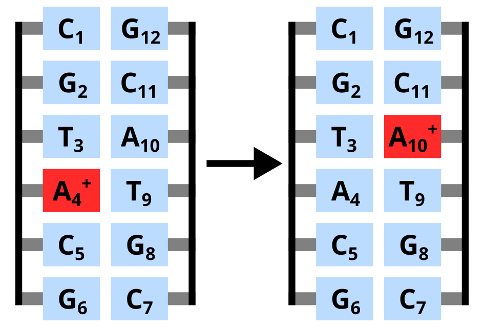
Figure 1: Schematic representation of the electron transfer studied. A radical cationic adenine is shown in red, whereas neutral ground state nucleobases are in blue. The equivalent process involving A${}_{10}^{+}$ in the initial state is also studied.

It should be emphasized that the structural relaxations occur on a rugged energy landscape in a multi-dimensional configuration space, which makes the visualization and the microscopic understanding of such processes difficult. Hence, we model the real non-equilibrium processes by means of non-equilibrium MD simulations, similarly to the studies of vibrational relaxations in pure liquid water^{45, 46}, or of protein quakes⁴⁷. The initial and final states may be connected via many reaction paths, and the high efficiency of today’s computer hardware and software makes it possible to generate abundance of non-equilibrium trajectories to sample the space of the reaction paths. This way, the undesired noise is filtered out by averaging of the trajectories in the space of suitable collective coordinates. The slow convergence of results that are to be averaged is accepted as an unfortunate fact, which is under full control, however. The technique is referred to as Reaction Path Averaging (RPA) throughout the paper, and its description is another aim of this work.

The paper is organized in two major parts dealing with the equilibrium and non-equilibrium simulations. Each of the parts starts with a description of the methodology used, and follows with the outcome of the respective analyses. In the final section, we conclude with a discussion of the results in the context of the previously reported work.

2 Equilibrium Ensembles

2.1 Methods of Equilibrium Simulations

The DNA oligonucleotide was described with the molecular mechanics (MM) force field Amber parm99bsc0 ^{48, 49}. The MM models of adenine in the radical cationic state was created by adjusting the Amber partial atomic charges of the ground state, to represent the electrostatic potentials obtained at the HF/6-31G* level via restricted electrostatic potential fitting (RESP) ⁵⁰ performed with the Antechamber module of AmberTools ⁵¹. Such an application of RESP is compatible with the Amber force field. Quantum chemical calculations were performed with Turbomole 6.5 ^{52, 53}. The difference between the adjusted cationic and ground state charges is sketched in Figure S1. The electronic change involves almost all of the adenine atoms.

Bond, angle, torsional and Lennard-Jones (LJ) parameters of the charged state were considered equal to their neutral ground state values. The use of ground-state LJ parameters is justified by the small deviations of Bader’s atomic volumes ^{54, 55} calculated at the HF/TZVP level. The root-mean-square deviations (RMSD) of atomic volumes from those in the ground state amount to 13 %. The largest deviation was found for one of the amino hydrogens (33 %). Such changes of atomic volumes would translate into changes of the LJ radii of at most 10 %, corresponding to ca. 0.2 Å; this is the maximal possible magnitude of differences of LJ radii that was neglected.

Regarding the bond, angle and torsional parameters, several reasons led us to keep them unchanged upon the electronic change. First, the energy minimized geometries of the neutral ground and the radical cationic states are almost identical at the B3LYP/6-31G* level; the RMSD of heavy-atom coordinates is as low as 0.03 Å. Second, it is unclear if and how the quantum effects on the distribution of bond lengths should be modeled in classical simulations. A rather typical treatment of covalent bonds in classical MD simulations, adopted also in the current work is to constrain their lengths to the respective force-field equilibrium values ⁵⁶, even though this seems to be less usual in the field of DNA simulation. Further, any structural analyses are performed in terms of collective coordinates, where nucleobases are represented as rigid bodies; the internal degrees of freedom are filtered out in any case. Finally, the aim is to describe mostly the interaction of a nucleobase with its environment, for which the intra-nucleobase degrees of freedom play little role.

The double-stranded DNA hexanucleotide d(CGTACG)₂ was immersed in a periodic box filled with ca. 3000 SPC/E water molecules ⁵⁷, and the system was neutralized by addition of ten sodium ions ⁵⁸, or nine whenever a radical cationic adenine was involved. The conformational space of the oligonucleotide with the radical cationic A${}_{4}^{+}$ or A${}_{10}^{+}$, and the neutral ground state (GS) adenines was sampled by means of ten independent equilibrium molecular dynamics (MD) simulations of at least 510 ns each, for every of the different DNA species. We note that the structure of an ionized DNA species may not be able to reach thermodynamic equilibrium due to the short lifetime of the cationic state. Still, the assumption that the cationic state lives long enough to make structural equilibration possible is a necessary one, and present in all of the cited previous simulation work. All of the simulations were performed with Gromacs 4.6 ^{59, 60}. The entire simulation setup is further detailed in the Supporting Information (SI).

In summary, the structural ensembles were generated with MD simulations in which bond lengths were constrained to their equilibrium values, while all of the remaining degrees of freedom including angles and dihedral angles were free to vary. For the purpose of any following structural analysis, rigid-body alignment of nucleobases was performed. Thus, intra-molecular degrees of freedom were integrated out effectively and were not analyzed. DNA structures were described in terms of the helical parameters within the standard reference frame as defined by Tsukuba conventions ⁶¹, which were calculated with the 3DNA program suite ⁶² interfaced to Gromacs by means of the do_x3dna utility ⁶³. The numpy ⁶⁴ and matplotlib ⁶⁵ libraries were utilized in most of the python analyses.

2.2 Equilibrium Structure

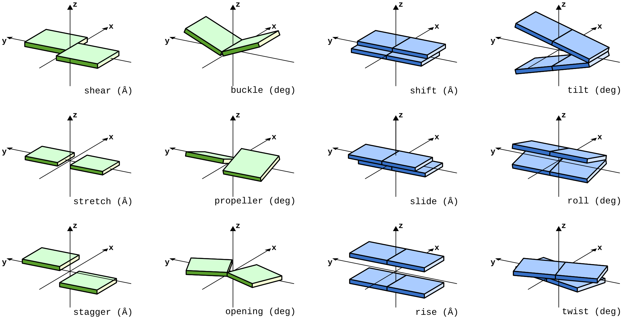
Figure S2: The collective coordinates for the description of DNA structure (a.k.a. helical parameters) ¹⁷ in the standard reference frame as defined by Olson et al.¹⁸. Each box represents a nucleobase. The parameters of base pairs are in green, and those of base-pair steps are blue.

The relatively high rigidity of nucleobases allows the atomistic representation of the DNA structure to be reduced into a few relevant coordinates ⁴⁴, here referred to as the helical parameters. They describe the relative orientation either of the nucleobases within a base pair, or of two consecutive base pairs, i.e. the base-pair step (see Figure S2).

We make use of the concept of helical parameters to describe the structure of the central TA step, which is involved in the electron transfer reaction investigated. Regarding the equilibrium states, mean values of the helical parameters over the equilibrium ensembles were calculated to infer the structural change of the central TA step associated with the electron transfer reaction. Note that mostly the mean values are discussed, and the variance and statistical uncertainty expressed in terms of the respective standard deviations and standard errors of the mean are presented in the SI. Apart from the helical parameters, the dihedral angles in the sugar-phosphate backbone and the sugar puckering were analyzed as well.

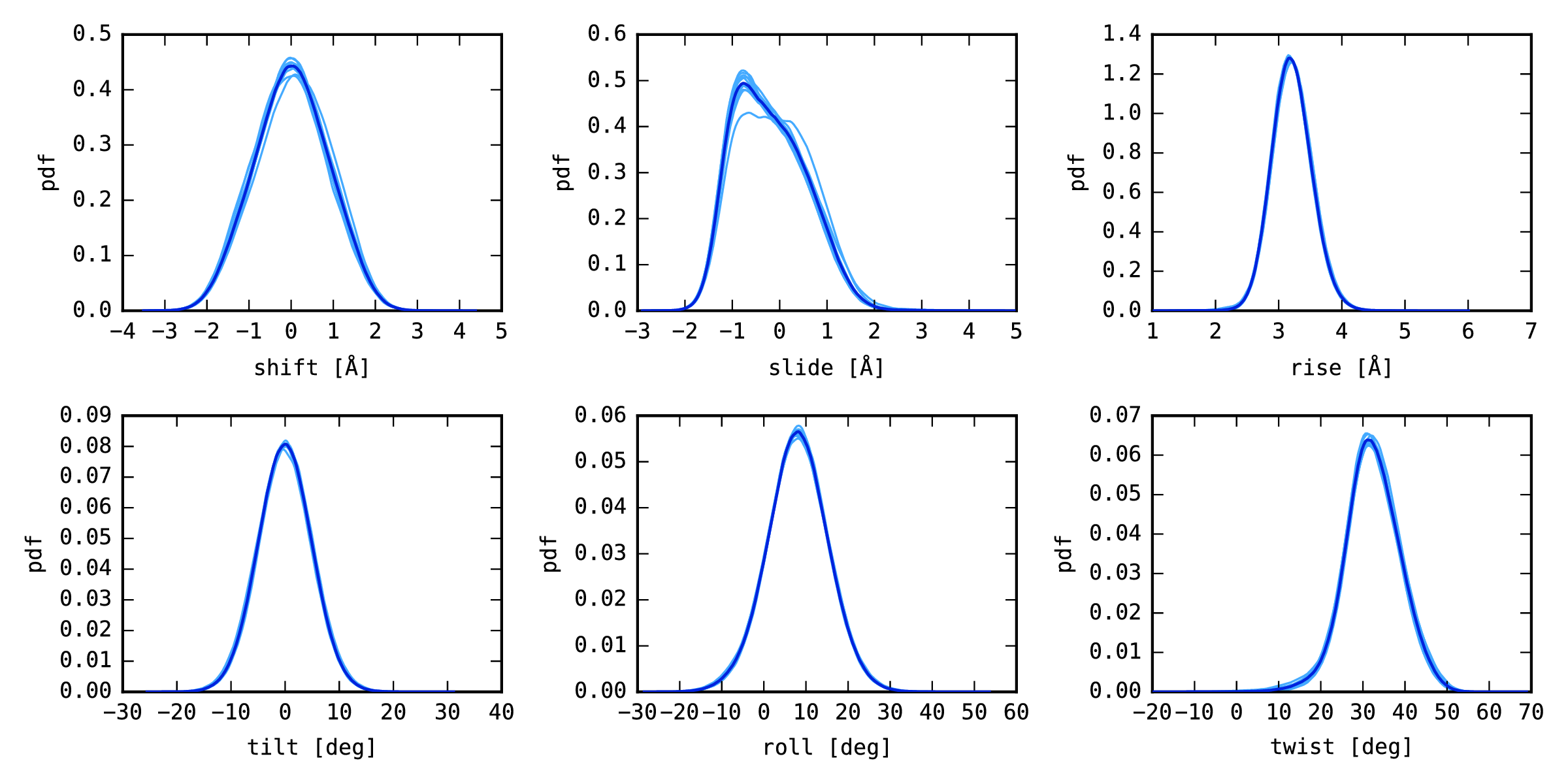
Figure S3: Probability density functions (pdf) of the parameters of the central base-pair step TA, shown for ten 510-ns-long trajectories (light blue), and for the aggregated ensemble (dark blue), where both adenines were in the ground electronic state.

The equilibrium structure of the central TA step with both adenines uncharged (in the neutral ground state) is in between the A- and B-DNA conformations; all of the helical parameters are summarized in Tables S2 and S3. In comparison with the sequence-averaged data from high-resolution crystal structures ⁶¹, the values of roll and twist are closer to A-like values, whereas the other helical parameters resemble a B-like conformation more closely (Table S3). While it is a known deficiency of current DNA force fields that they underestimate twist, the equilibrium values of twist lie within the error bars of both A-DNA and B-DNA here. The distributions of helical parameters are close to normal, see Figures S3–S4, with an exception of the slide, which hints at a bimodal distribution. We note that no particular DNA conformation is a priori assumed in any of the following discussions, and the conformational changes are rather described by the actual values of helical parameters.

We also analyzed the structure of the sugar moieties of the four nucleotides composing the TA base-pair step, see Tables 1, 2, S5 and S6. The canonical BI substate is dominant, with a propensity of 85 % and 96 % for the adenosines and the thymidines, respectively, and a mean lifetime of ca. 400 ps. The mean lifetime of the BII substate is ca. 70 ps and ca. 20 ps for the adenosines and the thymidines, respectively. Note, however, that the BI/BII equilibrium remains an open issue in general: “A reliable experimental estimate of the BII population remains so far a major challenge… Additional work is required to clarify the issue.”⁶⁶. The sugar puckering is rather diverse, with the canonical C2’-endo substate populated only to 33 % and 17 % in each of the two adenosines and each of the two thymidines, respectively. All of the sugar conformations are relatively short-lived, with mean lifetimes below 4 ps. A positive charge located on one of the adenines stabilizes the BI substate of its own backbone, whereas it destabilizes BI of the opposite strand; the propensity of BI changes from 85 % in the ground state to 99 % and 45 %, respectively (Tables 1 and S5). Likewise, the mean lifetime of BI of the charged adenosine increases to 3.5 ns, and that of the opposite adenine decreases to 165 ps (Table S5).

	T3	A10	A4	T9
GS	96	86	85	96
A${}_{4}^{+}$	32	44	99	96
A${}_{10}^{+}$	96	99	47	31

Table 1: Populations (in %) of the BI substate of the four nucleotides in the TA base-pair step. BI is considered whenever the difference of backbone dihedral angles $\varepsilon-\zeta<0$. The remainder to 100 % pertains to the BII substate.

	T3	A10	A4	T9
C1’-exo	36	31	32	35
C2’-endo	17	34	33	17
C3’-exo	1	10	10	1
C4’-exo	12	6	6	13
O4’-endo	32	17	17	33

Table 2: Populations (in %) of various conformations of the deoxyribose ring (i.e., sugar pucker) of the nucleotides in the TA base-pair step in the neutral ground electronic state. These data for DNA with A${}_{4}^{+}$ or A${}_{10}^{+}$ are presented in Table S7.

The structural changes upon electron transfer are rather minor at the level of individual base pairs (Table S2). Merely the changes of propeller and opening are non-negligible, amounting to 7.5^∘ and 5.5^∘, respectively, and reflecting well the sequence symmetry. For the global DNA conformation, however, the inter-nucleobase orientation is less important than the relative orientation of consecutive base pairs. Thus, we turn our attention to the changes of base-pair step parameters of the central TA step instead, and these are summarized in Table 3. The electron transfer is accompanied by a huge change of 3.4 Å in shift, which stands for a relative movement of two neighboring base pairs in the plane perpendicular to the helical axis in the direction from/to major/minor groove (Figure S2). This conformational change is seen clearly in the DNA structural models in Figure 3 constructed from the mean values of the helical parameters (Tables S2 and S3). The differences of slide and rise vanish. Among the angular parameters, the change in tilt is the most pronounced and amounts to 5.3^∘. The changes of roll and twist are close to zero. Hence, regarding the relaxations, we focus our attention to the changes of shift and tilt. The good convergence of the equilibrium ensembles is reflected by symmetric values of the relevant parameters as shown in Table 3. The standard errors of the mean are low, too (Tables S2–S4).

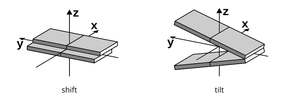
Figure 2: The DNA base-pair step parameters shift and tilt. Each box represents one nucleobase.

	$\mathrm{mean\,}\pm\mathrm{\,std}$	$\mathrm{sem}\times 10^{3}$
$\Delta$shift	$3.40\pm 1.25$	0.89
$\Delta$slide	$0.01\pm 0.73$	0.52
$\Delta$rise	$0.01\pm 0.42$	0.30
$\Delta$tilt	$5.32\pm 7.16$	5.10
$\Delta$roll	$-0.11\pm 9.74$	6.94
$\Delta$twist	$0.46\pm 8.34$	5.93

Table 3: The overall change in helical parameters of the central TA base-pair step during the reaction $\mathrm{A}_{4}^{+}\rightarrow\mathrm{A}_{10}^{+}$ as represented by differences of mean values (mean) calculated from the equilibrium ensembles equivalent to at least 5.1 $\mu$s. The variance and statistical uncertainty are quantified by means of the standard deviation (std) and the standard error of the mean (sem), respectively. Shift, slide and rise in Å; tilt, roll and twist in degrees. Note that the reaction $\mathrm{A}_{10}^{+}\rightarrow\mathrm{A}_{4}^{+}$ yields values that are the negative of those in the table due to symmetry. Equivalent data for the base-pair parameters are in Table S8. For the absolute values of the base-pair step parameters obtained for equilibrium structural ensembles, refer to Tables S3 and S4.

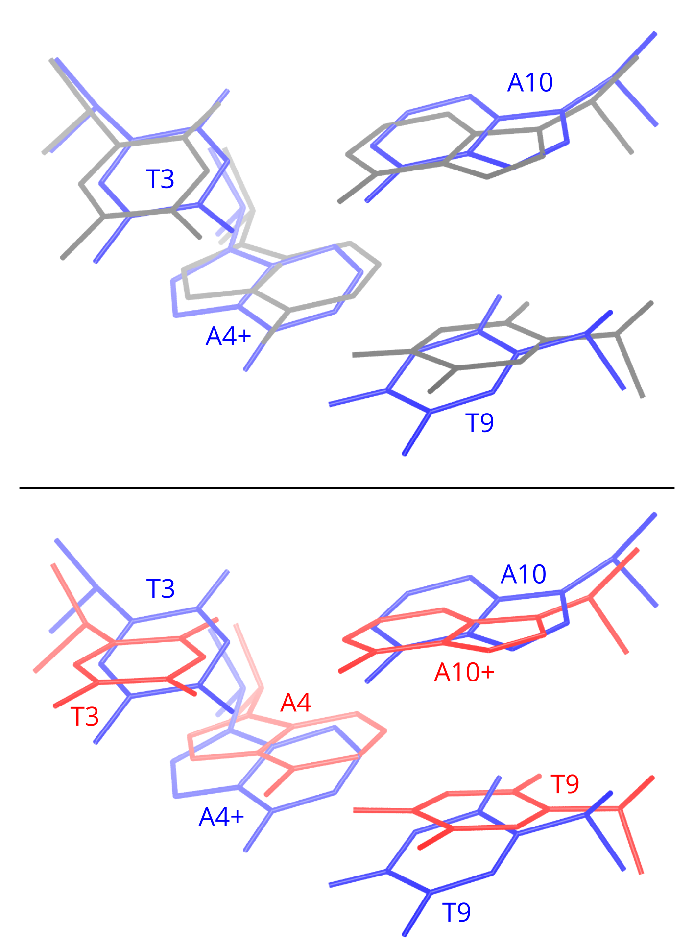
Figure 3: The average structures of the TA step with both adenines in the neutral ground state (gray), radical cationic A${}_{4}^{+}$ (blue), and radical cationic A${}_{10}^{+}$ (red). Hydrogen atoms are omitted for clarity.

Also interesting is to compare the above observations with the structural dependence of the electronic coupling between nucleobases, which is one of the determinants of electron transfer. Voityuk et al.⁶⁷ reported a strong dependence of electronic coupling on rise and slide, but almost none on shift and tilt, for the ((TA), (AT)) base-pair step involving uncharged nucleobases only. This is difficult to correlate with our findings above, thus no connection is apparent between the structural relaxation of DNA upon electron transfer and structural dependence of the electronic coupling.

2.3 Equilibrium Energetics

Motivated by the relation to TRSS experiments, the previous simulation studies concentrated mostly on the energy relations in the DNA molecule, between DNA and the solvent, and their response to the de-excitation of a component of the system (reviewed by Furse and Corcelli).⁶⁸ The equilibrium trajectories generated here may be analyzed to estimate the magnitude of energy that has to relax after an electron transfer event. This is performed by evaluating the MM component of the diabatic energy gap (DEG),

$$\mathrm{DEG}(t=0) =\left<E(2)\right>_{1}-\left<E(1)\right>_{1}=$$

$$=\left<E(2)-E(1)\right>_{1},$$ (1)

for the initial state (time $t=0$) of a process 1$\rightarrow$2, where $E(x)$ is the total potential energy evaluated with the Hamiltonian of state $x$, and $\left<\,\right>_{y}$ represents the averaging of energy over an equilibrium ensemble generated with the Hamiltonian of state $y$. DEG for the final state of that process follows in analogy,

$$\mathrm{DEG}(t=\infty) =\left<E(2)\right>_{2}-\left<E(1)\right>_{2}$$

$$=\left<E(2)-E(1)\right>_{2}.$$ (2)

Generally, DEG is a measure of the relative magnitude of intermolecular interactions exercised by two different electron distributions with the remainder of the same molecular structure. In the case of electron transfer with vanishing reaction energy, the DEG would correspond to the outer-sphere reorganization energy $\lambda$ in the context of Marcus’ theory of electron transfer ². Note that the reorganization energy for the process $\mathrm{A}_{4}^{+}\rightarrow\mathrm{A}_{10}^{+}$, for instance, is the difference of energy evaluated with the Hamiltonian of A${}_{4}^{+}$ for the ensemble of structures of A${}_{10}^{+}$ and that of A${}_{4}^{+}$,

$$\lambda=\left<E(\mathrm{A}_{4}^{+})\right>_{\mathrm{A}_{10}^{+}}-\left<E(\mathrm{A}_{4}^{+})\right>_{\mathrm{A}_{4}^{+}}.$$ (3)

The values of DEG obtained for the initial and final states of the considered reactions are shown in Table 4. DEG for the reactant and product states of the electron transfer processes amounts to 177 kJ mol^-1 (with the appropriate sign), and this value is in agreement with our previously reported reorganization energies obtained with a similar methodology for similar DNA species ⁶⁹. Note that if the purpose of these calculations was to estimate reorganization energies, the values should be scaled down by a factor of ca. 1.4 to correct for the neglect of electronic polarization in classical MD simulations ⁷⁰. A result that is more relevant for the current work, though, is the change of DEG when passing from the initial to the final state of each respective reaction considered. In the electron transfers, DEG passes from 177 kJ mol^-1 to –177 kJ mol^-1, i.e. it decreases by 354 kJ mol^-1.

In the following, DEG as a function of time is used to probe the response of interactions in the DNA-solvent system during the relaxation simulations.

	$\mathrm{mean}\pm\mathrm{std}$	sem
DEG(0)	$176.4\pm 540.2$	1.48
DEG($\infty$)	$-177.9\pm 539.6$	1.45

Table 4: Diabatic energy gap for the initial state, DEG(0), and for the final state, DEG($\infty$), of the electron transfer $\mathrm{A}_{4}^{+}\rightarrow\mathrm{A}_{10}^{+}$ obtained from the equilibrium ensembles. Mean values (mean), standard deviations (std), and standard errors of the mean (sem) are provided. Note that the reaction $\mathrm{A}_{10}^{+}\rightarrow\mathrm{A}_{4}^{+}$ yields identical values due to symmetry.

3 Relaxations

3.1 Methods of Relaxations

To investigate the time evolution of the structural and energetic changes, relaxation simulations of 20 ps each were started from the appropriate equilibrium ensembles, which had been created by taking snapshots from the multi-100ns equilibrium MD trajectories of the end states in regular time intervals, as depicted in Figure 4. The changes of electronic structures were modeled by means of instantaneous changes of the MM point charges of the adenines at time $t=0$. 50,000 relaxations were simulated for each of the electron transfers $\mathrm{A}_{4}^{+}\rightarrow\mathrm{A}_{10}^{+}$ and $\mathrm{A}_{10}^{+}\rightarrow\mathrm{A}_{4}^{+}$. To assess any slower response, additional relaxation simulations were performed: 500 simulations of 1 ns each, and 100 simulations of 10 ns each. The resulting RPA time series of energies and of helical parameters were obtained by averaging over the 100,000 shorter relaxations, as well as 1000 or 200 longer simulations, respectively.

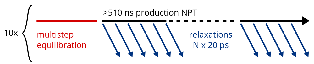
Figure 4: Non-equilibrium MD simulation scheme.

Each of the averaged data series was fitted with a multi-exponential function in order to estimate the relevant decay times. To this end, denser data from 20-ps-long simulations (with a time resolution of 2 fs) were combined with sparser data from 1-ns-long simulations (after block averaging over 50 data points, leading to the resolution of 100 fs). First, the longest relaxation time $\tau$ was determined with an exponential fit, $f(t)=w\exp[-t/\tau]$ to the 250–1000 ps region of the data series. The relaxation time $\tau$ was kept fixed then. In the second step, a more complex function composed of several, optionally stretched exponentials was fitted to the entire data series (0–1000 ps). The following function was considered,

$$f(t)= a_{1}\exp\left[-\frac{t}{t_{1}}\right]+a_{2}\exp\left[-\left(\frac{t}{t_{2}}\right)^{\!\!c_{2}}\right]+$$

$$+a_{3}\exp\left[-\left(\frac{t}{t_{3}}\right)^{\!\!c_{3}}\right]+a_{4}\exp\left[-\frac{t}{\tau}\right],$$ (4)

with the second and third exponential optionally stretched. The relaxations of the normalized energies (see below) employed a boundary condition of $a_{1}+a_{2}+a_{3}+a_{4}=1$. The relaxation of DNA helical parameters was fitted with a triple exponential (and $a_{3}=0$); the coefficients $a_{i}$ have the dimension of the helical parameter being fitted (ångström for shift, degree for tilt), and their sum $a_{1}+a_{2}+a_{4}$ shall correspond to the total magnitude of the relaxation shown in Table 3. A comparison of the multiple tested choices of optionally stretched exponentials can be found in the SI.

Prior to fitting, the baselines obtained from the equilibrium simulations were used to shift all of the relaxation data series to zero at infinite time. All of the fitting was performed with the Levenberg–Marquardt non-linear least-squares algorithm ^{71, 72} as implemented in the R package.^{73, 74} The initial guess of the parameters for fitting, and the fitted values for the ten individual sub-ensembles for each relaxation are presented in the SI. For every fitted exponential component, a decay time $T_{i}$ was obtained. For simple exponentials, $T_{i}$ equals directly to the parameter $t_{i}$; for stretched exponentials, this is calculated as $T_{i}=t_{i}/c_{i}\cdot\Gamma(1/c_{i})$ with the gamma function $\Gamma(x)=\int_{0}^{\infty}y^{x-1}\exp[-y]\,\mathrm{d}y$. The accuracy of the obtained fits was judged by the ratio of the residual sum of squares and the total sum of squares, RSS/TSS. Its calculation is described in the SI, as is the method to estimate the statistical uncertainty of determination of the fitting parameters.

3.2 Energy relaxation

We monitored the time course of energy relaxation with the time-dependent diabatic energy gap, which was obtained along the trajectory from every relaxation simulation 1$\rightarrow$2 as $\mathrm{DEG}(t)=E(2,t)-E(1,t)$, where $E(x,t)$ is the potential energy obtained with the Hamiltonian of state $x$ at time $t$ in the simulation. Then, these time series were averaged over the respective sets of relaxation simulations. Finally, DEG($t$) was normalized to the interval $(0,1)$ yielding the normalized diabatic energy gap (DEGN):

$$\mathrm{DEGN}(t)=\frac{\mathrm{DEG}(t)-\mathrm{DEG}(\infty)}{\mathrm{DEG}(0)-\mathrm{DEG}(\infty)}.$$ (5)

DEGN is very similar to the quantities employed previously for electric potentials by Maroncelli and Fleming ²⁵ as well as for differential interaction energies by Sen et al. ³¹ and Furse and Corcelli^{41, 68}. An advantage of our approach involving the non-equilibrium simulations is the fact that the needed baselines DEG(0) and DEG($\infty$) were determined accurately in the preceding equilibrium simulations, so that they need not be estimated with any, possibly difficult fitting. Note that the difficulties of determining the baselines with a sufficient accuracy constitute two of the “three factors that complicate the comparison of the experimental TRSS to the simulated [quantities]” within the linear response approximation ³¹.

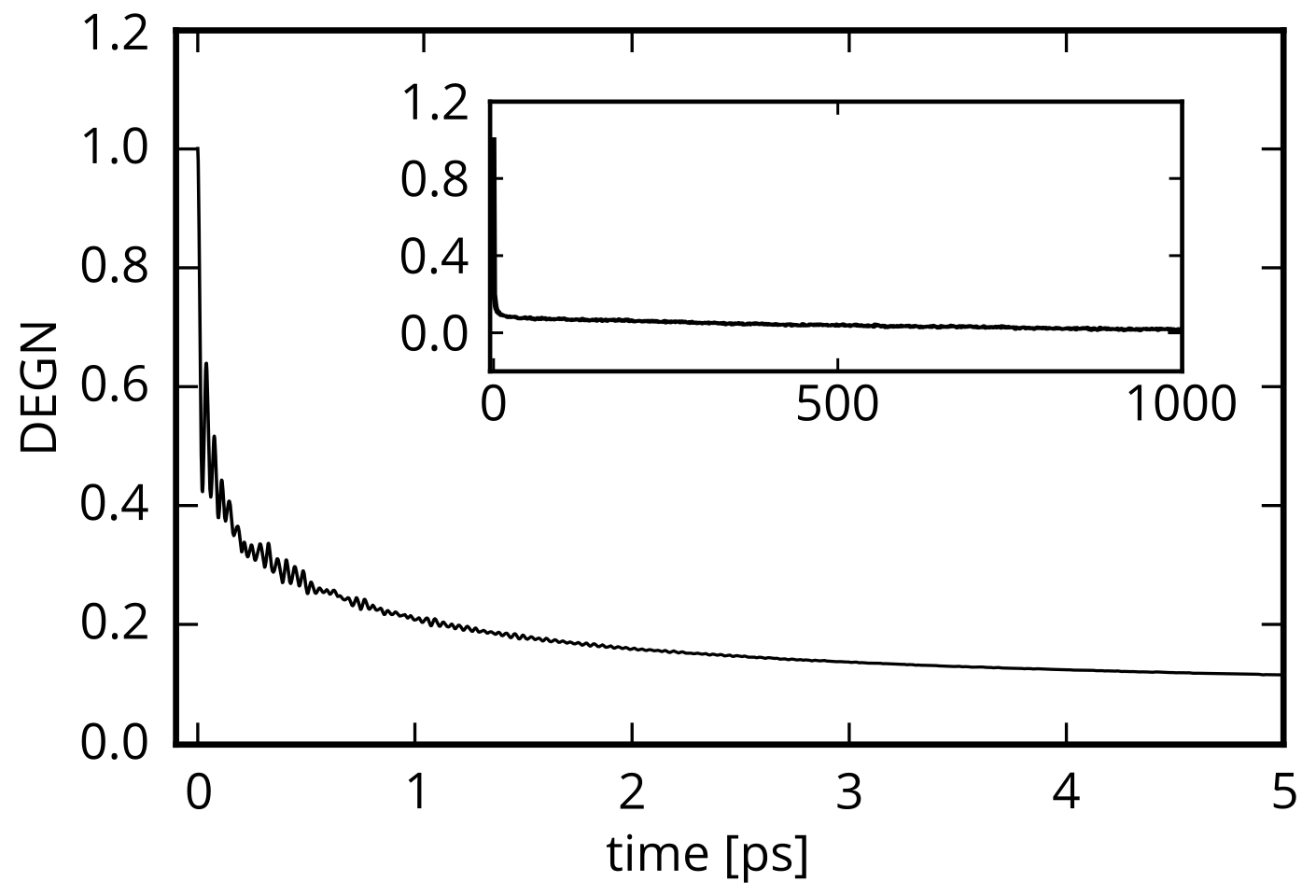
Figure 5: Energy decay as captured by the normalized diabatic energy gap (DEGN) following an instantaneous electron transfer. Data were obtained by averaging over the respective numbers of non-equilibrium MD simulations, see the main text. The inset shows the relaxation on a longer time scale.

The resulting averaged relaxation of DEGN is presented in Figure 5; note that every data point in this plot was obtained by averaging of 2$\times$50,000 values. The initial phase of the decay is very steep, and about 80% of the relaxation occurs within the first picosecond. The relaxation up to ca. 0.5 ps is apparently modulated by a periodic function with a small amplitude and a period of about 45 fs, which corresponds to the wavenumber of 740 cm^-1. This frequency is in the range of the librational motion of bulk water molecules ³⁰, Previously, such fluctuations were shown to induce fluctuations of instantaneous ionization energies of DNA nucleobases ³⁶.

No consensus seems to exist about what kind of analytic function represents the response in the best way. For instance, exponential, multi-exponential, stretched exponential or power-law functions have been proposed in the context of relaxations upon electronic changes in biomolecules ^{75, 28, 39, 76}. In this work, a sum of two exponentials and two stretched exponentials in Eq. 4 provided an accurate fit of the averaged DEGN decay over the interval of 1 ns. It turned out that the periodic oscillations in the DEGN data are too weak to be fitted, therefore no periodic component was considered.

	$a_{1}$	$t_{1}$	$a_{2}$	$t_{2}$	$c_{2}$	$a_{3}$	$t_{3}$	$c_{3}$	$a_{4}$	$\tau$	RSS/TSS
DEGN	0.34	0.0080	0.37	0.198	0.516	0.21	1.43	0.488	0.08	654	0.0076
uncert.	0.03	0.0004	0.11	0.052	0.090	0.08	1.62	0.104	0.01	95

Table 5: Values of the parameters from the fitting of a multi-exponential function to the data series of DEGN from the simulations of electron transfer; $t_{i}$ in ps, dimensionless numbers otherwise. The accuracy of the fit (RSS/TSS) and the estimates of uncertainty of the individual parameters were obtained as described in SI.

	Magnitude	Decay Time
	[%]	[ps]
1	34	0.0080
2	37	0.374∗
3	21	2.99∗
4	8	654
∗ stretched exponential

Table 6: Relaxation times of DEGN and their relative magnitudes.

The resulting parameters of the fitting function as well as the summary of decay times and the corresponding decay magnitudes are presented in Tables 5 and 6. First, there is an ultra-fast component with a large magnitude and a decay time around 10 fs. This agrees with the results from previous non-equilibrium simulations by Furse and Corcelli,⁴¹ who analyzed a smaller number of more coarsely sampled trajectories, while “any sub-100-fs components in these dynamics [were] unresolved”³³ in typical TRSS experiments. Then, there are two components with sizable magnitudes and decay times of 0.4 and 3 ps. Lastly, there is a relatively weak component with a sub-nanosecond decay.

The experiments by Zewail et al. reported decay times of a nucleobase analogue de-excitation of 1.4/1.0 and 19/10–12 ps (Ref. 32/Ref. 33). The relaxations upon electron transfer are somewhat faster, by factor of about three. We note that such a comparison is not quite straightforward: The decay in our simulations is a response to an electron transfer reaction. On the other hand, the experimental TRSS decays represent a response to a de-excitation of a DNA component or of another molecule bound to DNA. Importantly, recent reports suggested that the excitation/de-excitation of adenine is accompanied by a charge transfer from/to neighboring nucleobase(s) ^{16, 77}, and that the electronic re-arrangement upon (measured) de-excitation is delocalized just like it is upon (simulated) electron transfer. Therefore, just like the simulations in the current work, the TRSS experiments involved a response to a charge transfer process, albeit quantitatively different (i.e., with different quantitative characteristics like spatial extent, driving force or reorganization energy). The comparison of the current results to those from the TRSS experiments referred to above is justified from this point of view. In addition, to the best of our knowledge, no more closely related experimental data are available.

The discussion of DEGN will be resumed in Section 3.3 as soon as the relaxation of structural coordinates is presented.

3.3 Structural Relaxation

To characterize the relaxation of DNA structure upon electron transfer, the base-pair and base-pair step parameters were monitored along each of the relaxation trajectories, and these time series were averaged over both sets of trajectories. Owing to the symmetry of the self-complementary DNA sequence, the two reactions investigated are equivalent, $\mathrm{A}_{4}^{+}\to\mathrm{A}_{10}^{+}$ and $\mathrm{A}_{10}^{+}\to\mathrm{A}_{4}^{+}$. The corresponding relaxation simulations describe the same physical phenomenon, and must lead to the same results. Therefore, the time series obtained from the respective pairs of relaxation simulations were combined prior to analysis in order to improve the signal-to-noise ratio.

Figure 6: Time evolution of the base-pair step parameters shift and tilt. Note that the actual values for reactions $\mathrm{A}_{4}^{+}\rightarrow\mathrm{A}_{10}^{+}$ and $\mathrm{A}_{10}^{+}\rightarrow\mathrm{A}_{4}^{+}$ have opposite sign owing to the symmetry of the DNA sequence and the anti-symmetry of shift and tilt. For clarity, the values of parameters for $\mathrm{A}_{10}^{+}\rightarrow\mathrm{A}_{4}^{+}$ were inverted before plotting.

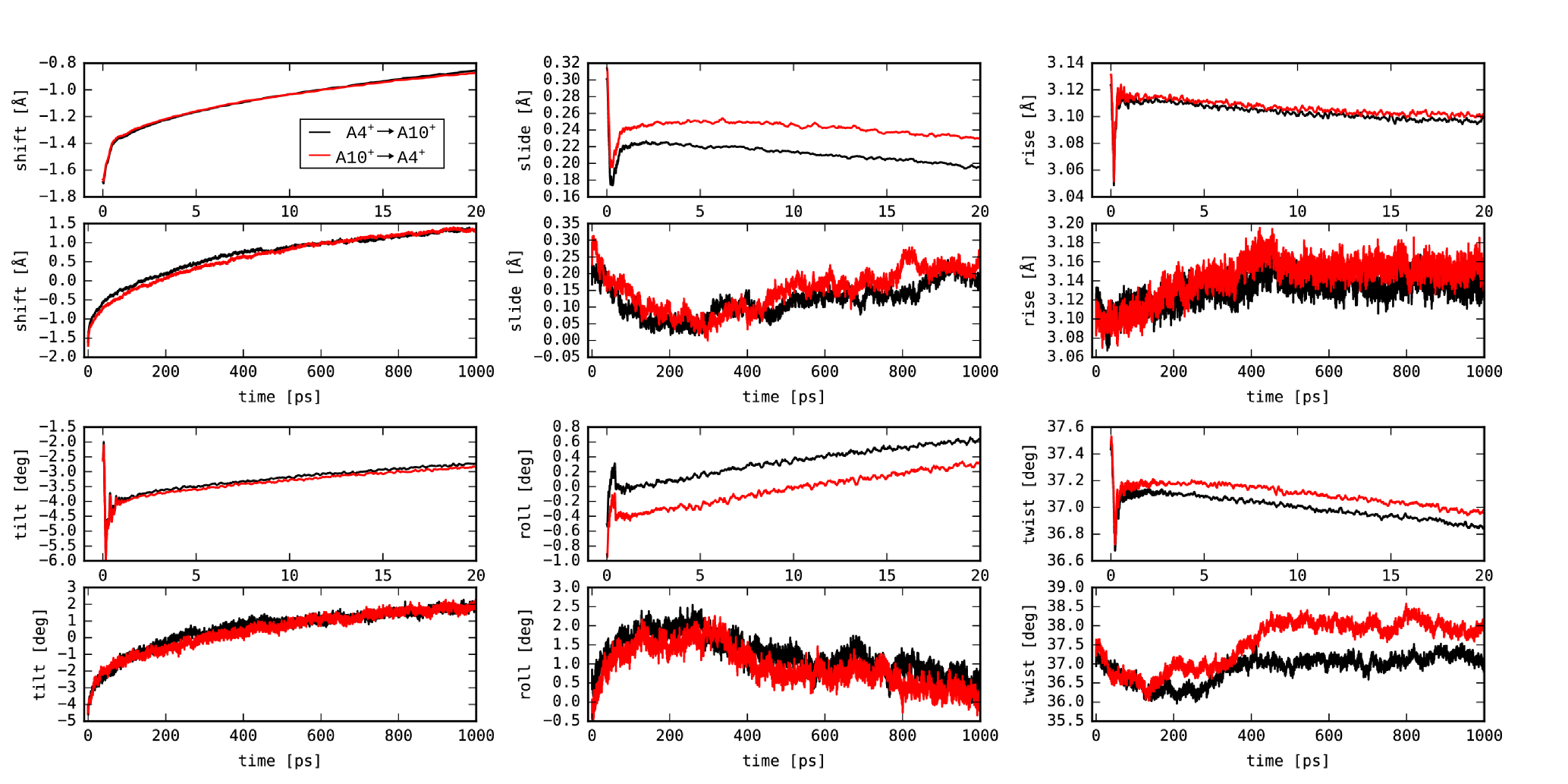
Figure S6: Time evolution of the base-pair step parameters following the electron transfer. Note that the actual values of shift and tilt for A₄- and A₁₀-involving reactions have opposite sign owing to the symmetry of the DNA sequence and anti-symmetry of the respective parameters. For clarity, the values of parameters involving A₁₀ were inverted before plotting.

Focusing on the most dynamical structural parameters as identified by the equilibrium ensembles, the relaxations of shift and tilt are shown in Figure 6; refer to Figure S6 for the full set of relaxation profiles. Immediately after the instantaneous electron transfer at $t=0$, within the first picosecond, both shift and tilt as well as all of the other parameters undergo strong fluctuations due to the sudden increase of energy in the system and its consequent redistribution. This immediate response of the DNA is followed by a slower relaxation, directed towards the final parameter values predicted from the equilibrium simulations.

Because of the symmetry of the considered palindromic DNA sequence, the black and the red curves in Figure 6 should be identical. This is not entirely the case; the differences of shift of up to 0.02 Å between the two instances are observed. Such a difference illustrates the extremely slow convergence of the non-equilibrium data with respect to the number of simulations performed. Still, the shape of the pairs of curves is remarkably similar, especially on the short time scale.

The decays of shift and tilt were subject of a fitting procedure as detailed above. A sum of two exponentials and one stretched exponential provided the best fit. The initial phase of the relaxation was particularly difficult to fit, and there were especially large oscillations in the case of tilt at the start of the electron transfer relaxation simulations (see Figure 6). These oscillations brought the averaged tilt from the initial value of $-2.7^{\circ}$ to $-6.0^{\circ}$, which is actually further away from the final equilibrium value of $+2.7^{\circ}$. Thus, the true magnitude of relaxation of tilt was ca. 8.7^∘, markedly larger than the above determined difference of equilibrium values of 5.32^∘. Since these initial oscillations cannot be fitted with any exponential-based function easily, the time $t=0$ was set to 164 fs for tilt, where it reaches the global minimum; the fitted function does not describe the initial oscillations consequently. The results of fitting are presented in Tables 7 and 8.

	$a_{1}$	$t_{1}$	$a_{2}$	$t_{2}$	$c_{2}$	$a_{4}$	$\tau$	RSS/TSS
Shift	0.27	0.281	1.28	55.5	0.568	1.89	603	0.00033
uncert.	0.02	0.078	0.30	20.1	0.071	0.33	41
Tilt	1.48	0.133	3.28	61.4	0.633	3.53	685	0.0019
uncert.	0.13	0.088	0.97	59.9	0.180	0.88	171

Table 7: Values of the parameters from the fitting of multi-exponential functions to the averaged data series of shift and tilt from the relaxation simulations of electron transfer; $t_{i}$ in ps, $a_{i}$ in ångström and degrees for shift and tilt, respectively, $c_{2}$ dimensionless. The estimates of uncertainty were obtained as described in the SI.

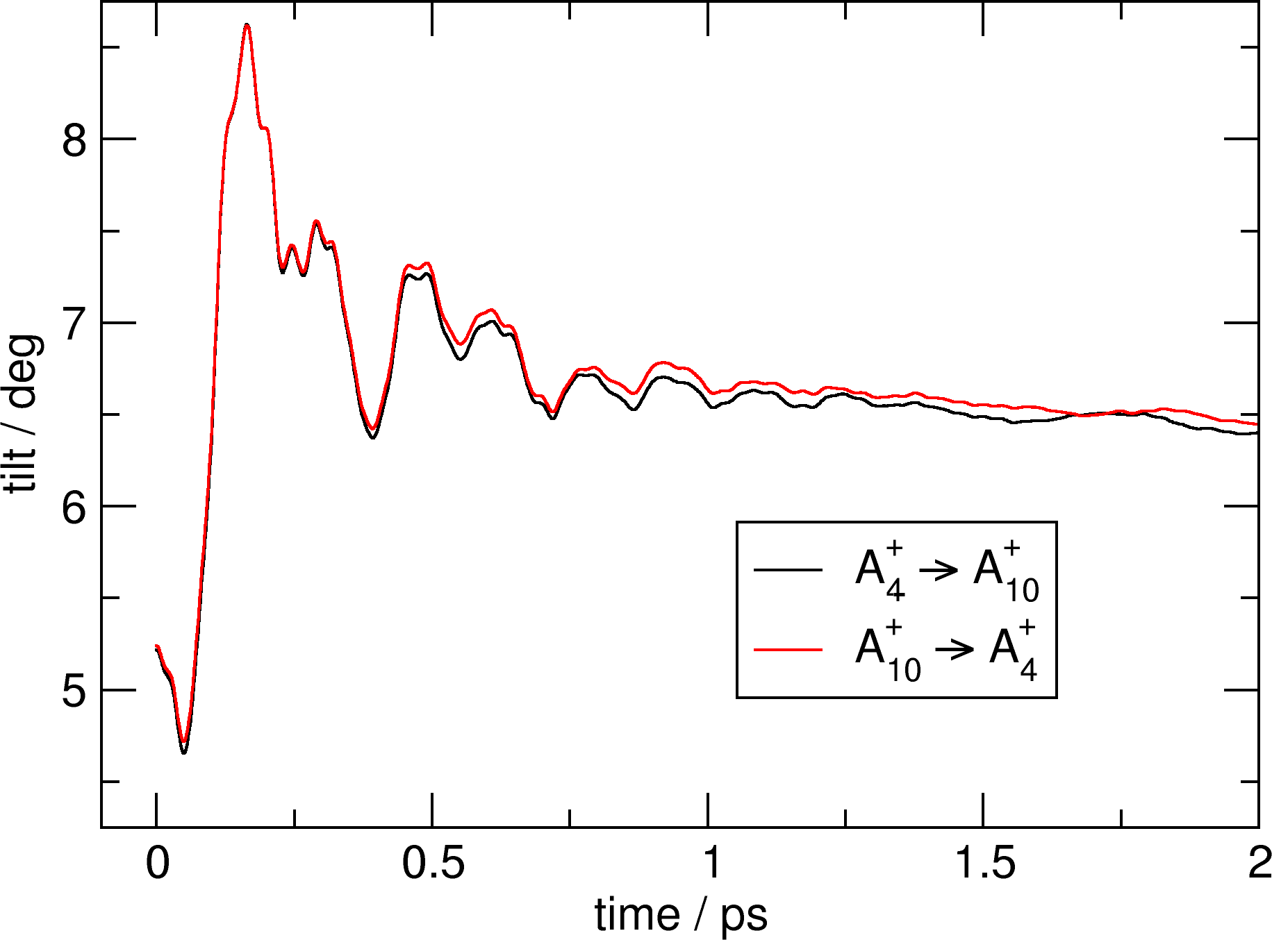
Figure S5: Relaxation of the tilt in the first 2 ps of the electron transfer simulations.

	Shift		Tilt+
	Magnitude	Decay Time	Magnitude	Decay Time
	[%]	[ps]	[%]	[ps]
1	8	0.281	18	0.133
2	37	90.1∗	40	86.5∗
3	55	603	43	685
∗ stretched exponential
+ To fit the tilt, $t=0$ is set at 164 fs, where the tilt reaches the global minimum due to the initial oscillation, see Figure S5. The relaxation is considered to start at this point.

Table 8: Decay times and relative magnitudes of the individual exponential components of the decays of shift and tilt.

The observed decay times are presented graphically in Figure 7. When comparing the decays of helical parameters, representing the structure of DNA, to the decay of DEGN, a striking difference is that there is no ultra-fast decay component in the former. Recall that the relaxation of DEGN in Section 3.2 contained a dominant component with a decay time in the femtosecond range and magnitude of 34 %. Apparently, there is no active ultra-fast relative movement of nucleobases that would be responsible for this part of the DEGN decay. It may be concluded that rather than the DNA modes of motion, the dynamics of solvent molecules are responsible, for instance the librational movements of water molecules.

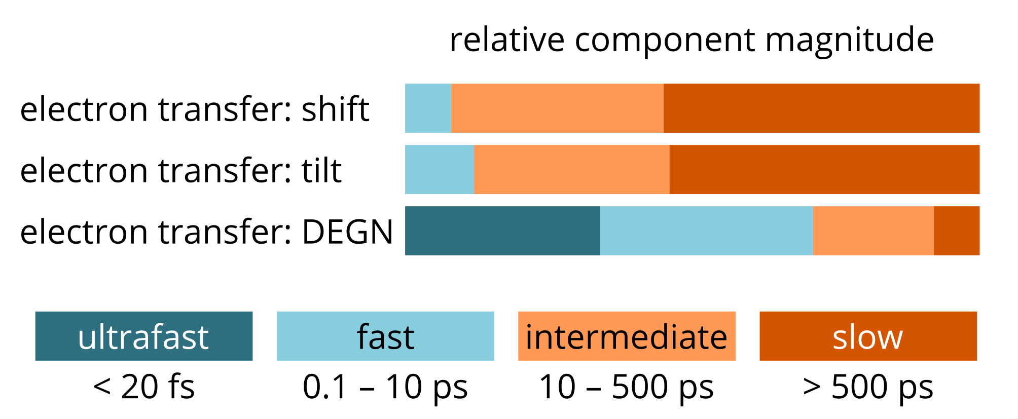
Figure 7: Relative magnitudes of the various decay time classes obtained for all of the relaxations investigated.

The structural relaxations are characterized by three kinds of relaxations: i) a minor fast decay time of 0.1–0.3 ps, ii) a major intermediate one of about 90 ps, and iii) a major slow one of 600–700 ps. These observations are markedly different from the relaxation profiles of DEGN: The ultra-fast component, extremely pronounced in DEGN, is missing altogether in the structural decays. Further, the sub-picosecond relaxation has the lowest magnitude of the observed components. And finally, the slowest, nanosecond components possess a much higher relative importance in the structural relaxation than in the DEGN relaxation.

Markedly, the slow component of the structural decay, responsible for a quite large portion of the decay of both shift and tilt, agrees with the slowest decay component of DEGN perfectly: the decay times are 603 and 685 ps for shift and tilt, respectively, while DEGN decays in 654 ps. This comparison suggests that the longest relaxation time observed for DEGN (representing the interaction energies) is due to the dynamics of the DNA molecule itself, as opposed to the shorter relaxation times, which may be ascribed to the solvation dynamics. This scenario agrees with the interpretation of TRSS data collected for DNA by Sen et al., who stated that only 4 % of the electric field correlations comes from the DNA ³¹. In the current work, 8 % of DEGN is attributed to the DNA for the electron transfer. A possible interpretation is that the closest solvent molecules respond rapidly to electron transfer, accompanied by hardly any change of the structure of the DNA itself. Only after a longer time, the DNA structure relaxes finally on two different time scales (90 ps and 600–700 ps), possibly together with an additional portion of the solvent.

Obviously, the different modes of motion of DNA and other components of the system, prominently, the solvent, contribute to the changes of energy with different strengths. There are even some structural changes that do not contribute to the monitored energetics, which are simulation analogs of TRSS decays, at all. Thus, no simple relationship can be deduced between the decay of energy and the decay of structural parameters of DNA.

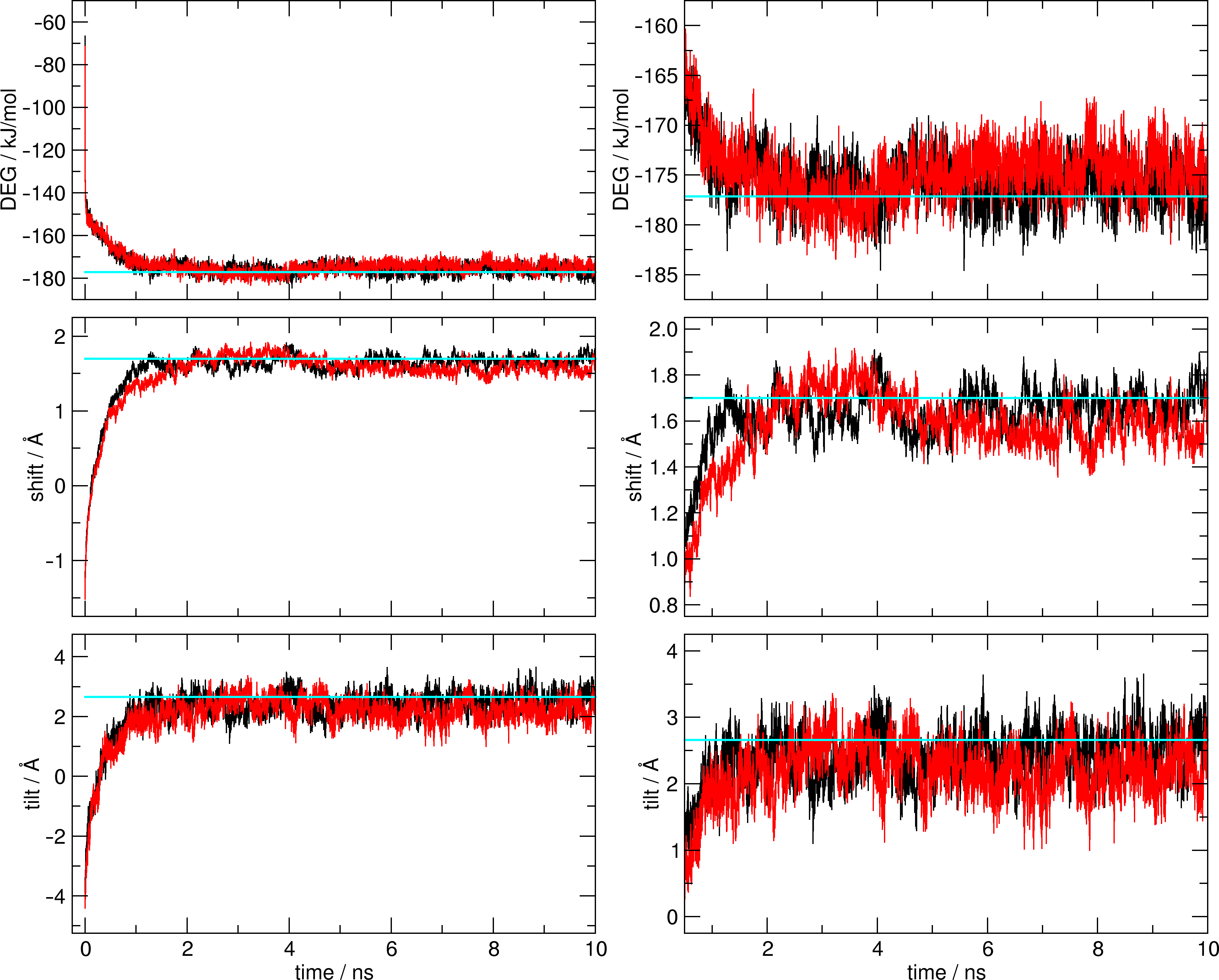
Figure S9: Relaxation of DEGN (top), shift (center) and tilt (bottom) following the electron transfer reactions $\mathrm{A}_{4}^{+}\to\mathrm{A}_{10}^{+}$ (black) and $\mathrm{A}_{10}^{+}\to\mathrm{A}_{4}^{+}$ (red; sign was inverted before plotting for shift and tilt). The cyan line depicts the equilibrium value of the final state.

All of the decay times were determined on the basis of non-equilibrium simulations of a length of 1 ns, which turned out to be similar to the longest decay time. Hence, it may be that any possible slower relaxation pattern is hard to detect. To verify such possibility, additional extended simulations were performed, namely 100 simulations of 10 ns each for the relaxation following each of the electron transfer reactions $\mathrm{A}_{4}^{+}\to\mathrm{A}_{10}^{+}$ and $\mathrm{A}_{10}^{+}\to\mathrm{A}_{4}^{+}$. All of the simulation parameters were the same as in the simulations of 1 ns. The resulting relaxation profiles are presented in Figure S9. No slower processes were observed, thus the lists of decay times in Tables 6 and 8 may be considered complete.

3.4 Reaction Path Averaging

Results from the simulations described above have constituted a basis for an analysis of the structural relaxation of DNA upon electron transfer between two nucleobases, called here RPA, which has proceeded in the following steps:

1. A few coordinates of interest, or collective variables were defined. These are the base-pair step helical parameters of the central TA step, and shift and tilt were shown to be the most significant.

2. These coordinates were recorded along a large number of realizations of an irreversible process, here, the relaxation of DNA structure described with classical MD simulation.

3. The resulting time series of the collective variables were averaged. Because of the extremely strong variation of molecular structures in the ensembles of irreversible simulations, the above discussion of characteristic decay times was only made possible by averaging of a huge number of MD trajectories generated.

4. The averaged time series were analyzed further. The decay times and magnitudes in Section 3.3 were obtained with fitting of multi-exponential functions to the individual time series of collective variables. Additionally, the time series were used to investigate correlations between the chosen collective variables, and to visualize the studied irreversible process, specifically here, the averaged structural relaxation of DNA.

The averaged time series of the shift and the tilt are shown in correlation diagrams in Figure 8, together with time series from a few examples of the many individual non-equilibrium trajectories. Two features are apparent immediately:

The time series of shift and tilt in the individual non-equilibrium trajectories are scattered all over the diagrams largely. They are extremely different from each other, thus they compose an overwhelmingly noisy ensemble and do not reveal any correlation of shift and tilt whatsoever. This vast structural variance is then removed by virtue of averaging, which makes apparent the time course of the relaxation of shift and tilt, and, in addition, their correlation.

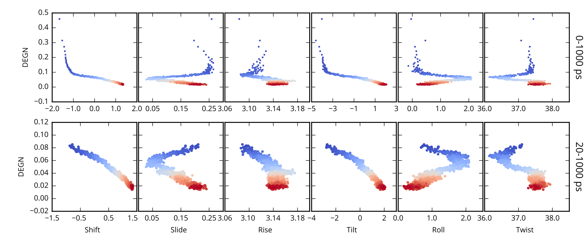
Figure S8: Correlation diagrams of DEGN with all of the helical parameters of the central TA base-pair step with the adenine in the radical cation state. The time is color coded from blue to red. The plots in the bottom row start at the time of 20 ps.

Indeed, the averaged time series (blue-to-red in Figure 8) reveals a strong linear correlation of shift and tilt, with a coefficient of determination of $R^{2}=0.99$. This is identical to a previous observation of the relaxation of shift and tilt proceeding on the same time scales and with the same relative magnitudes (Table 8), repeated from another perspective. The correlation of shift and tilt actually implies that the relaxation of DNA structure proceeds, for the most part, along a single collective variable represented by the linear combination of shift and tilt. Correlations are also observed for other pairs of helical parameters, see Figure S7; interestingly, these are often non-linear, exhibiting more complex shapes. The same is true for the correlation of relaxation profiles of DEGN with those of the helical parameters, see Figure S8. Most importantly, any correlations between the individual collective variables are only apparent after averaging of a large volume of non-equilibrium data.

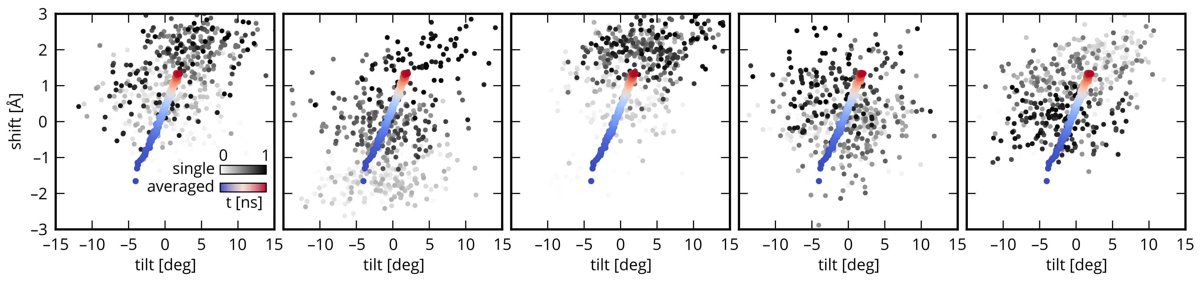
Figure 8: The correlation of the base-pair step parameters shift and tilt following the electron transfer $\mathrm{A}_{4}^{+}\rightarrow\mathrm{A}_{10}^{+}$. Time series from five individual trajectories are time-coded from white to black; the averaged data are time-coded from blue to red. Similar correlation plots for all of the other pairs of helical parameters may be referred to in Figure S7.

The dynamics of the atomistic structure of the molecule can be re-constructed from the averaged time series of the collective variables. Here, the time series of the helical parameters were translated into time-dependent coordinates of each atom, and were visualized, see the video clips in SI.

The first one (relaxation.mp4 in SI) captures the initial oscillations of the central base-pair step following an instant transfer of a full electron between two adenines. The strong structural fluctuations dissipate within the first picosecond, being followed by a slower relaxation mostly in the shift coordinate, compare with Figure 6. This movement proceeds in the direction of the final conformation, as obtained from equilibrium simulations (shown in pale green).

The other video (transfer.mp4 in SI) shows structural distortions of a longer dsDNA oligonucleotide accompanying a sequential electron transfer along the molecule. This visualization was constructed from DNA structures with helical parameters obtained for the equilibrium states of the DNA molecule. All of the long double helix except one base pair contained neutral adenines, and the remaining one was considered as radical cation, which was transferred along the DNA helix in a sequential manner. For every elementary transfer event, the helical parameters were switched from the equilibrium values of the initial state to those of the final state instantly. Thus, the relaxation is considered instantaneous in this representation in contrast to the detailed picture of a single base-pair step above. The purpose of this video clip is to provide an idea of possible change of structure of DNA during long-distance electron transfer.

4 Discussion and Conclusions

We compare the time course of relaxation of DEGN as the probe of energy relations in the system on the one hand, and the structural relaxation represented for the most part by the helical parameter shift, on the other. Since the relaxation is multi-modal and several individual “energy modes” are observed in DEGN, we investigate the possibility to identify each of the them with any of the modes of motion of the DNA. In case no such mode is found, we would assume modes of motion of the solvent to be responsible. (Clearly, the current work cannot discriminate between the effects of water and counterions as discussed previously.)^{39, 31}

The DEGN response observed in the current work is in accordance with the previously reported components. First, there is a high-amplitude ultra-fast decay time of 8 fs, which agrees well with the fastest component reported previously ³⁹. Two further sizable contributions of 1 ps and 10–12 or 20 ps were reported for de-excitation by Zewail et al.^{32, 33}. A somewhat faster relaxation is observed following the electron transfer, with decay times of 0.37 and 3.0 ps. Third, there is a minor component with decay times of 650 ps, which does not seem to correspond to any modes of motion discussed previously in the context of hydration dynamics.

Three decay modes were found in the structural relaxations, with decay times of 0.1–0.3 ps, 90 ps and 600–700 ps. The first and second mode differ from the decay times of DEGN clearly, while the slowest one is especially interesting. Although its relative importance in the DEGN relaxation is much lower than in the helical parameters, the remarkable similarity of the corresponding decay times for DEGN and helical parameters suggests that the longest relaxation time observed for DEGN is actually due to the dynamics of the DNA molecule itself. This is opposed to the shorter relaxation times, for which the solvation dynamics is most likely responsible; a similar conclusion was drawn previously by Sen et al.³¹. Thus, the resulting picture of the relaxation energetics, or the TRSS decay, is that the response of the closest solvent molecules drives its fastest component(s), and the decay of the relaxation of DNA structure modulates the energies or TRSS on a longer time scale reaching a nanosecond.

Another important observation is more general: the different modes of motion contribute to the changes of energy differently, and some structural changes do not contribute to energies at all. For instance, the fastest and second-fastest mode of decay of shift and tilt are clearly inactive in the DEGN decays. Thus, there is no linear relationship between the decay of energy and the decay of structural parameters.

We also recall the meaning of DEG here. It is the difference of potential energy in the system, obtained with the Hamiltonians corresponding to the initial and final state of the relaxation. In our scheme, this reduces to the interaction energy of the difference of atomic charges between the initial and final state with the entire remainder of the molecular system (other nucleobases, DNA backbone and the solvent). Thus, effectively, this quantity corresponds closely to the quantities used in the previous simulation studies, e.g. the difference of excited- and ground-state interaction energy ⁶⁸ or the effective transition interaction energy ³¹; by contrast, Pal et al. ^{39, 40} considered simply the total ground-state interaction energy.

4.1 Limitations of the Model

Let us discuss the important approximations employed in our methodology. It should be emphasized that all of them apply to the previous simulation studies cited throughout this work, as well.

In our simulations, perfectly equilibrated initial states of the investigated processes were considered. In reality, however, a radical cationic adenine may exhibit a shorter lifetime; note the reported rate of electron transfer from one adenine to another of 4 or 20 ns^-1 in some DNA sequences ^{78, 79}, slightly faster than the slowest relaxation process. Consequently, a full structural relaxation of DNA would take a longer time to complete than an electron transfer. Thus, the real structural distortions may be smaller in magnitude than the values in this work, which represent the upper bounds of structural and energetic changes.

Another assumption is that the electron transfer reaction takes place with exactly the same probability for every molecular structure in the equilibrium ensemble. In reality, however, some configurations would be preferred, mostly because of more appropriate activation energies, represented for instance by the difference of instantaneous ionization energies close to zero. This effect would be by far more time consuming to describe, while more simplified approaches based on MM-only calculations of electric potentials are conceivable. Difficulties may arise from the possibly inefficient sampling of the configurations with high probability of electron transfer, which may be rare events.

Also, the electron transfer process is considered to be instantaneous, or infinitely fast, and is modeled by a sudden and complete switch of MM atomic charges. It is unclear how electron transfer occurs in reality from the microscopic point of view. Note that this information does not seem to be accessible from experiments, nor is covered by the classical theories of electron transfer like Marcus’ theory, and cannot be predicted by the current non-adiabatic simulation schemes reliably ³⁸.

Generally, the application of an empirical force field comes with all of its advantages and drawbacks. (i) The recent parm99bsc0 force field used in this work describes the structure of DNA in a robust way, while some of its features could still be improved ⁸⁰. (ii) The derivation of atomic charges of the excited adenine molecule was designed to resemble the recommended RESP methodology for ground state as closely as possible, thus the adenine parameters are compatible with the remaining components of the force field. (iii) What classical MD simulation can never do is to describe the dynamics of covalent bonds, mainly its quantum character. This is one of the reasons why the MD simulations in this work were performed with all bond lengths constrained. Consequently, any ultra-fast response of the DNA structure that would be due to relaxation of bond lengths cannot be described. Still, it is possible to consider the magnitude of energy relaxation for which the change of bond lengths is responsible to be equal or smaller than the inner-sphere reorganization energy for electron transfer. The value for purine nucleobases is 0.23 eV,³⁷ which represents 6 % of total energy relaxation, thus, we consider this effect minor. Also, we performed additional simulations of 4 $\mu$s of aggregated sampling, having constrained only bonds involving hydrogen atoms. The helical base-pair step parameters and their fluctuations, see Table S4, differ hardly from those obtained with all bonds constrained, thus we consider the latter treatment justified. (iv) Another phenomenon impossible to describe is any interference of the dynamics of the nucleobase with the change of electron density modeled by a set of fixed partial charges.

4.2 Benefits

Importantly, the methodology of the current study evinces several advantageous points, novel in comparison with previous works.

Most significantly, the true relaxation process is modeled by performing non-equilibrium simulations. This is in contrast to, and an improvement when comparing with most of the cited previous work by other authors, who usually performed equilibrium simulations to describe non-equilibrium processes within a linear response approximation. There is no need for this transition in the current work.

The magnitudes of any structural changes are obtained from extensive equilibrium MD simulations. Additionally, in this way, we provide the absolute values of baselines for the relaxation profiles conveniently, which are normally inaccessible via (auto)correlations. This is particularly true about the structural parameters, whose changes can be then converted to atomic models and visualized in a straightforward way.

In addition, the reaction path averaging concept was used to highlight the movements of DNA and visualized them in two videos clips. Itself, the idea of averaging non-equilibrium trajectories is not new. In 1990, Levy et al. investigated the relaxation of aqueous solvation shell of a formaldehyde molecule upon its de-excitation ⁸¹. By means of averaging of 80 MD trajectories, it was possible to identify the major mode of relaxation, which was the translational motion of water molecules. Laage and Hynes analyzed 16,000 hydrogen bond flipping events observed in an equilibrium MD simulation of pure water, which made it possible to propose a jump mechanism of water re-orientation ²⁶. Some of the features of our RPA analysis resemble this previous work – the introduction of suitable collective variables as well as averaging of time series obtained for a large number of realizations of the process of interest. Most recently, the averaging of 10,000 non-equilibrium classical MD simulations was used to infer energy dissipation in myoglobin after CO photodissociation ⁴⁷. In this work, the reaction was also modeled via instantaneous change of molecular mechanical force field.

Let us discuss the applicability of the RPA approach as implemented in this work to non-equilibrium chemical processes in a more general context. There are a few requirements on the studied problem, and our application to processes taking place in double-stranded DNA serves as an example of how they may be fulfilled.

Obviously, a suitable computational method for the description of the process of interest has to be available. The current work made use of classical force field-based MD simulations, which is perhaps the most convenient tool. Applications to non-equilibrium processes involving, e.g., extensive changes of electronic structure like re-arrangements of chemical bonding may require passing to quantum chemical or hybrid QM/MM methodologies.

A sufficient number of non-equilibrium simulations has to be performed to yield converged results. The number of simulations needed may easily become huge, placing excessive requirements on resources in terms of computational efficiency as well as storage space. Fortunately, these calculations can be run in parallel trivially.

It seems to be favorable if the process of interest can be described by means of (a small number of) collective variables or reaction coordinates. This work benefited from the helical parameters for DNA being available. Also, the initial and final states should be characterized first, for two reasons: Fires, a structural ensemble of the initial state is needed to provide initial conditions for the non-equilibrium simulations. And second, it is a good idea to have estimated the extent of the total change of the selected collective variables during the process investigated. This information decreases the number of fitting parameters for the time decays, and makes it possible to judge the convergence of the non-equilibrium simulations to the ensemble of the final state.

4.3 Summary and Outlook

In summary, the structural changes in a double-stranded DNA oligonucleotide upon an electron transfer between two nucleobases were characterized. The dominant mode of motion is the helical parameter shift of the involved base-pair step. The interaction energy decay following such a reaction were characterized as well. The contribution due to the dynamics of the aqueous solvent seems to be dominant, while the relaxation of the DNA structure manifests itself on a longer time scale. The RPA approach provided a unique illustration of DNA conformational changes, which would be otherwise difficult to visualize. Combined with a suitable choice of collective variables, RPA may become an attractive approach to characterize and visualize non-equilibrium chemical processes in general.

Finally, there are a few directions in which this research may be extended. For the specific application to DNA electron transfer, the modes of motion of the surrounding water molecules are of particular interest. Therefore, a future RPA analysis may involve the solvation shell of the nucleobases, described with appropriate coordinates, or collective variables likely involving many water molecules. An appropriate way to extend the RPA approach itself is to implement a weighting of the individual non-equilibrium trajectories according to the propensity of the initial structures to undergo the reaction. Upon this modification, RPA will become an even more realistic description of the non-equilibrium process.

Supporting Information

Additional information on the simulation setup and the performed analyses; detailed characterization of the equilibrium structure of the DNA molecule involving the various states of the adenine nucleobase – ground-state neutral, and radical cation; additional graphical representation of the relaxation data; results from alternative multi-exponential fits to relaxation data; estimates of accuracy and uncertainty of fitting; correlation diagrams of the DNA helical parameters in the course of relaxation; two RPA videos depicting the relaxation of DNA structure upon electron transfer; full author lists of Refs. 51, 61, 82, and 80.

We thank Filip Lankaš for critical comments and valuable suggestions, and we appreciate the encouragement by Pavel Hobza. MHK is thankful for support provided by the Alexander von Humboldt Foundation. This research was also supported by the bwHPC initiative and the bwHPC-C5 project, funded by the Ministry of Science, Research and the Arts Baden-Württemberg (MWK) and the Research Foundation of Germany (DFG), through the associated compute services of the JUSTUS HPC facility located at the University of Ulm.

TOC Graphic

Supporting Information to
“Reaction Path Averaging:
Characterizing Structural Response
of the DNA Double Helix
to Electron Transfer”

5 Methods

5.1 Simulation Box

The atomic structure of a double-stranded DNA hexanucleotide with the palindromic sequence d(CGTACG)₂ was prepared in the canonical B-DNA conformation with the Nucleic Acid Builder. The DNA was placed in a periodic rhombic dodecahedron box. The size of the box was chosen to ensure a distance of at least 1.2 nm between the DNA molecule and any box face. The box was filled with ca. 3000 water molecules, and 10 water molecules were replaced by sodium ions to compensate for the negative charge of DNA. The box contained 9427 atoms in total.

The DNA was described with the Amber ff99bsc0 parameter set ^{1, 2}, translated into the Gromacs file format with the ambconv utility ³. In order to avoid any possible fraying of the terminal base pairs, harmonic restraints with a force constant of 2000 $\mathrm{kJ\,mol^{-1}\,nm^{-2}}$ were applied on the heavy atoms of the three cytosine$\ldots$guanine hydrogen bonds of both terminal base pairs (i.e., CYT:N3$\ldots$GUA:N1, CYT:O2$\ldots$GUA:N2 and CYT:N4$\ldots$GUA:O6, using the Amber naming convention). The three-site SPC/E water model was used ⁴ because it yields reasonable dynamic properties of bulk water as expressed in terms of self-diffusion coefficient and dielectric constant, much better than e.g. the related TIP3P model does ⁵. The sodium ions were modeled with parameters by Joung and Cheatham ⁶.

The adenine nucleobases were treated in a special way. The standard Amber ff99bsc0 charges were used for the ground state, whereas modified charges were used for charged state (Figure S1). Three distinct simulation setups were employed, as summarized in Table S1. Whenever one of the adenines was charged, one of the sodium atoms was made neutral to maintain electroneutrality. Ten independent equilibrium simulations differing in the initial velocities were run for each type of simulation setup.

abbrev	A4 charges	A10 charges
GS	ground state	ground state
A${}_{4}^{+}$	charged	ground state
A${}_{10}^{+}$	ground state	charged

Table S1: Summary of simulation boxes.

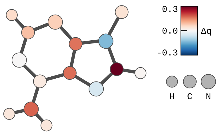
Figure S1: The difference between partial atomic charge differences of the charged and ground state (i.e. the default Amber ff99bsc0).

5.2 Simulation Setup

The following set of equilibration simulations were performed for each simulation setup:

• 1500 steps of conjugated gradient (CoG) energy minimization using a steepest descent step every 10 CoG steps.

• Assignment of random initial velocities from the Maxwell-Boltzmann distribution at 10 K.

• $5\cdot 10^{5}$ steps of constant-volume water heating to 300 K using the v-rescale thermostat ⁷ with a coupling time of 0.2 ps. The solute was kept at 10 K with an additional thermostat with the same coupling time.

• $1\cdot 10^{5}$ steps of constant-volume heating to 300 K. Two separate v-rescale thermostats with the coupling time of 0.5 ps were used for the solute and solvent.

• $5\cdot 10^{5}$ steps of constant-pressure simulation at 300 K and 1 bar. Two separate v-rescale thermostats with a coupling time of 0.5 ps were used together with a single the Berendsen barostat ⁸ with a coupling time of 0.5 ps.

• $2\cdot 10^{6}$ steps of constant-pressure simulation at 300 K and 1 bar using a single Nosé-Hoover thermostat ^{9, 10} ($\tau=0.5$ ps) and the Parrinello-Rahman ¹¹ barostat ($\tau=0.5$ ps).

• The electrostatics were treated with the Particle Mesh Ewald algorithm ¹² with a direct-space cut-off of 1.1 nm and a maximum grid spacing of 0.12 nm. The Lennard-Jones interactions were cut off at 1.1 nm. A long-range correction for energy and pressure ¹³ was applied. The equations of motion were integrated by means of the leap-frog algorithm with a time step of 1 fs (NVT simulations) or 1.5 fs (NPT simulations). All bond lengths were constrained with p-LINCS ⁵⁶.

For each simulation setup, ten independent trajectories differing in the initial velocities were generated. The production runs performed with the Nosé-Hoover thermostat ($\tau=1$ ps) and the Parrinello-Rahman barostat ($\tau=1$ ps) were extended to at least $3.4\cdot 10^{8}$ steps of 1.5 fs, corresponding to 510 ns. All of the other simulation parameters were identical to the last equilibration step. A full-precision trajectory frame of the entire simulation box was stored every 15 ps in order to initiate non-equilibrium relaxations.

The non-equilibrium simulations were done at constant temperature of 300 K and pressure of 1 bar using identical setup as in the equilibrium simulations. A time step of 1 fs was used for time propagation, while all coordinates were saved every 2 fs. The simulations were carried out with the Gromacs 4.6.7 program package ^{15, 16}.

5.3 Definitions of Statistical Descriptors

5.3.1 Mean Value

The mean value $\left\langle A\right\rangle$ of a quantity $A$ (e.g. helical parameter Shift), measured for each frame $i$ of each of the trajectory $t$, was calculated for the entire ensemble by equation S1.

$$\left\langle A\right\rangle=\frac{1}{N}\sum_{t}^{N}\frac{1}{N_{f,t}}\sum_{i}^{N_{f,t}}A_{i},$$ (S1)

where $N$ is the number of trajectories (i.e. 10), and $N_{f,t}$ is the number of frames for a given trajectory (typically about 350,000). Each frame of each of the trajectories was taken with the same weight, so the mean value could also be expressed by equation S2.

$$\left\langle A\right\rangle=\frac{1}{N_{f}}\sum_{i}^{N_{f}}A_{i},$$ (S2)

where $N_{f}$ is the total number of frames in the ensemble.

5.3.2 Standard Deviation

The standard deviation $\mathrm{std}(A)$ of a quantity $A$ (e.g. helical parameter Shift), measured for each frame $i$, was calculated for the entire ensemble by equation S3.

$$\mathrm{std}(A)=\sqrt{\frac{1}{N_{f}}\sum_{i}^{N_{f}}\left(A_{i}-\left\langle A\right\rangle\right)^{2}},$$ (S3)

where $N_{f}$ is the total number of frames and $\left\langle A\right\rangle$ stands for the mean value (Equation S2).

5.3.3 Standard Error of the Mean

The standard error of the mean $\mathrm{sem}(A)$ of a quantity $A$ (e.g., helical parameter Shift), measured for each frame $i$, was calculated for the entire ensemble by equation S4.

$$\mathrm{sem}(A)=\frac{\mathrm{std}(A)}{\sqrt{N_{f}}},$$ (S4)

where $N_{f}$ is the total number of frames and $\mathrm{std}(A)$ stands for the standard deviation as calculated by equation S3.

5.3.4 Difference of Mean Values

The difference $\Delta A$ of two quantities $A_{1}$ and $A_{2}$ (e.g. helical parameter Shift of the excited-state and ground-state ensembles, $\Delta$Shift) was calculated as a difference of the mean values of the final $\left\langle A_{2}\right\rangle$ and initial $\left\langle A_{1}\right\rangle$ states (equation S5).

$$\Delta A=\left\langle A_{2}\right\rangle-\left\langle A_{1}\right\rangle.$$ (S5)

5.3.5 Standard deviation of the Difference

The standard deviation $std(\Delta A)$ of a difference of two quantities $A_{1}$ and $A_{2}$ (e.g. helical parameter Shift of the excited-state and ground-state ensembles, $\Delta$Shift) was calculated from the standard deviations of the two quantities over all ensembles by equation S6.

$$\mathrm{std}(\Delta A)=\sqrt{\mathrm{std}(A_{1})^{2}+\mathrm{std}(A_{2})^{2}}$$ (S6)

5.3.6 Standard Error of the Mean Difference

The standard error of the mean of a difference $\mathrm{sem}(\Delta A)$ of two quantities $A_{1}$ and $A_{2}$ (e.g., helical parameter Shift of the excited-state and ground-state ensembles, $\Delta$Shift) was calculated as a sum of standard errors of the mean of each of the quantities following equation S7.

$$\mathrm{sem}(\Delta A)=\mathrm{sem}(A_{1})+\mathrm{sem}(A_{2})$$ (S7)

6 Results and Discussion

6.1 Schematic Representations of Helical Parameters

6.2 Equilibrium Simulations

6.2.1 Helical Parameters

	T3-A10 pair		A4-T9 pair
	$\mathrm{mean}\pm\mathrm{std}$	$\mathrm{sem}\times 10^{3}$	$\mathrm{mean}\pm\mathrm{std}$	$\mathrm{sem}\times 10^{3}$
Shear	$-0.04\pm 0.37$	0.2	$0.05\pm 0.34$	0.2
Stretch	$0.00\pm 0.14$	0.1	$0.00\pm 0.14$	0.1
Stagger	$0.15\pm 0.42$	0.2	$0.15\pm 0.42$	0.2
Buckle	$-1.65\pm 11.49$	6.0	$1.45\pm 11.50$	6.0
Propeller	$-12.01\pm 8.60$	4.5	$-12.01\pm 8.64$	4.5
Opening	$-0.08\pm 6.20$	3.2	$-0.05\pm 6.24$	3.3

Table S2: Mean values (mean), standard deviations (std) and standard errors of the mean (sem) of the helical parameters of the two central TA base pairs calculated from the ground-state equilibrium trajectories.

	simulations		A-DNAa	B-DNAa
	$\mathrm{mean}\pm\mathrm{std}$	$\mathrm{sem}\times 10^{3}$	$\mathrm{mean}\pm\mathrm{std}$	$\mathrm{mean}\pm\mathrm{std}$
Shiftb	$0.01\pm 0.89$	0.5	$0.00\pm 0.54$	$-0.02\pm 0.45$
Slide	$-0.21\pm 0.77$	0.4	$-1.53\pm 0.34$	$0.23\pm 0.81$
Rise	$3.21\pm 0.32$	0.2	$3.32\pm 0.20$	$3.32\pm 0.19$
Tiltb	$-0.03\pm 4.97$	2.6	$0.1\pm 2.8$	$0.1\pm 2.5$
Roll	$8.01\pm 7.28$	3.8	$8.0\pm 3.9$	$0.6\pm 5.2$
Twist	$32.34\pm 6.60$	3.4	$31.1\pm 3.7$	$36.0\pm 6.8$
a sequence-averaged data from X-ray crystallography 61
b should be zero due to helix anti-symmetry

Table S3: Mean values (mean), standard deviations (std) and standard errors of the mean (sem) of the helical parameters of the central TA base-pair step calculated from the ground-state equilibrium trajectories.

	$\mathrm{A}_{4}^{+}$		$\mathrm{A}_{10}^{+}$		$\mathrm{A}_{4}^{+}$ (flexi)
	$\mathrm{mean}\pm\mathrm{std}$	$\mathrm{sem}\times 10^{3}$	$\mathrm{mean}\pm\mathrm{std}$	$\mathrm{sem}\times 10^{3}$	$\mathrm{mean}\pm\mathrm{std}$	$\mathrm{sem}\times 10^{3}$
Shift	$-1.70\pm 0.89$	0.5	$1.70\pm 0.88$	0.4	$-1.80\pm 0.84$	0.5
Slide	$0.31\pm 0.52$	0.3	$0.33\pm 0.52$	0.3	$0.37\pm 0.48$	0.3
Rise	$3.12\pm 0.30$	0.2	$3.13\pm 0.29$	0.1	$3.14\pm 0.30$	0.2
Tilt	$-2.64\pm 5.07$	2.6	$2.68\pm 5.06$	2.5	$-3.04\pm 5.00$	3.1
Roll	$-0.56\pm 6.90$	3.5	$-0.67\pm 6.87$	3.4	$-0.83\pm 6.84$	4.2
Twist	$37.39\pm 5.99$	3.1	$37.85\pm 5.79$	2.9	$37.84\pm 6.20$	3.8

Table S4: Mean values (mean), standard deviations (std) and standard errors of the mean (sem) of the helical parameters of the central TA base-pair step calculated from the equilibrium trajectories with radical-cation adenine. The last two columns (A${}_{4}^{+}$ flexi) represent the trajectories obtained with flexible bonds between heavy atoms.

6.2.2 Sugar Puckering and Backbone Substates

	T3	A10	A4	T9
GS	417.2$\pm$926.5	466.3$\pm$1012.6	439.4$\pm$922.0	387.5$\pm$873.1
A${}_{4}^{+}$	16.4$\pm$53.6	158.6$\pm$432.8	3552.3$\pm$6210.3	1279.2$\pm$3136.0
A${}_{10}^{+}$	1288.4$\pm$3283.4	3585.9$\pm$5961.1	171.0$\pm$492.7	16.3$\pm$50.7

Table S5: Life times of the BI backbone substate in the form of mean value $\pm$ standard deviation. Derived from the equilibrium data.

	T3	A10	A4	T9
GS	18.7$\pm$63.6	73.7$\pm$243.9	75.7$\pm$233.3	17.5$\pm$66.0
A${}_{4}^{+}$	35.5$\pm$94.2	206.2$\pm$530.9	38.5$\pm$144.1	46.4$\pm$144.7
A${}_{10}^{+}$	47.8$\pm$142.2	33.6$\pm$118.0	189.5$\pm$486.5	36.1$\pm$77.7

Table S6: Life times of the BII backbone substate in the form of mean value $\pm$ standard deviation. Derived from the equilibrium data.

pucker	T3	A10	A4	T9
A${}_{4}^{+}$
C1’-exo	52	48	8	52
C2’-endo	31	31	54	36
C3’-exo	0	4	35	1
C4’-exo	7	4	1	2
O4’-endo	10	12	2	10
A${}_{10}^{+}$
C1’-exo	51	7	48	52
C2’-endo	36	54	32	31
C3’-exo	2	35	4	0
C4’-exo	2	1	4	6
O4’-endo	10	2	12	10

Table S7: Populations (in %) of the different deoxyribose ring conformations (i.e., sugar pucker) of the nucleobases in the central base pair step in charged states.

6.2.3 End-State Changes of Helical Parameters

	T3-A10		A4-T9
	mean$\pm$std	$\mathrm{sem}\times 10^{3}$	mean$\pm$std	$\mathrm{sem}\times 10^{3}$
$\Delta$Shear	$0.27\pm 0.50$	0.4	$0.24\pm 0.64$	0.5
$\Delta$Stretch	$-0.06\pm 0.21$	0.1	$-0.06\pm 0.21$	0.1
$\Delta$Stagger	$0.15\pm 0.57$	0.4	$0.16\pm 0.57$	0.4
$\Delta$Buckle	$0.88\pm 15.47$	11	$1.19\pm 15.45$	11
$\Delta$Propeller	$7.88\pm 12.20$	8.7	$-7.23\pm 12.06$	8.6
$\Delta$Opening	$5.70\pm 8.36$	5.9	$-5.35\pm 8.39$	5.9

Table S8: Overall change in helical base-pair parameters of the third T₃-A₁₀ and fourth A₄-T₉ base pairs upon $\mathrm{A}_{10}^{+}\rightarrow\mathrm{A}_{4}^{+}$ reaction as represented by differences of mean values (mean) calculated from the equilibrium ensembles equivalent to at least 5.1 $\mu$s each. Standard deviations (std) and standard errors of the mean (sem) are also provided. Shear, stretch and stagger in Å; buckle, propeller and opening in degrees. Note that the $\mathrm{A}_{10}^{+}\rightarrow\mathrm{A}_{4}^{+}$ reaction yields negative values of $\mathrm{A}_{4}^{+}\rightarrow\mathrm{A}_{10}^{+}$ by definition.

6.3 Equilibrium Probability Density Functions

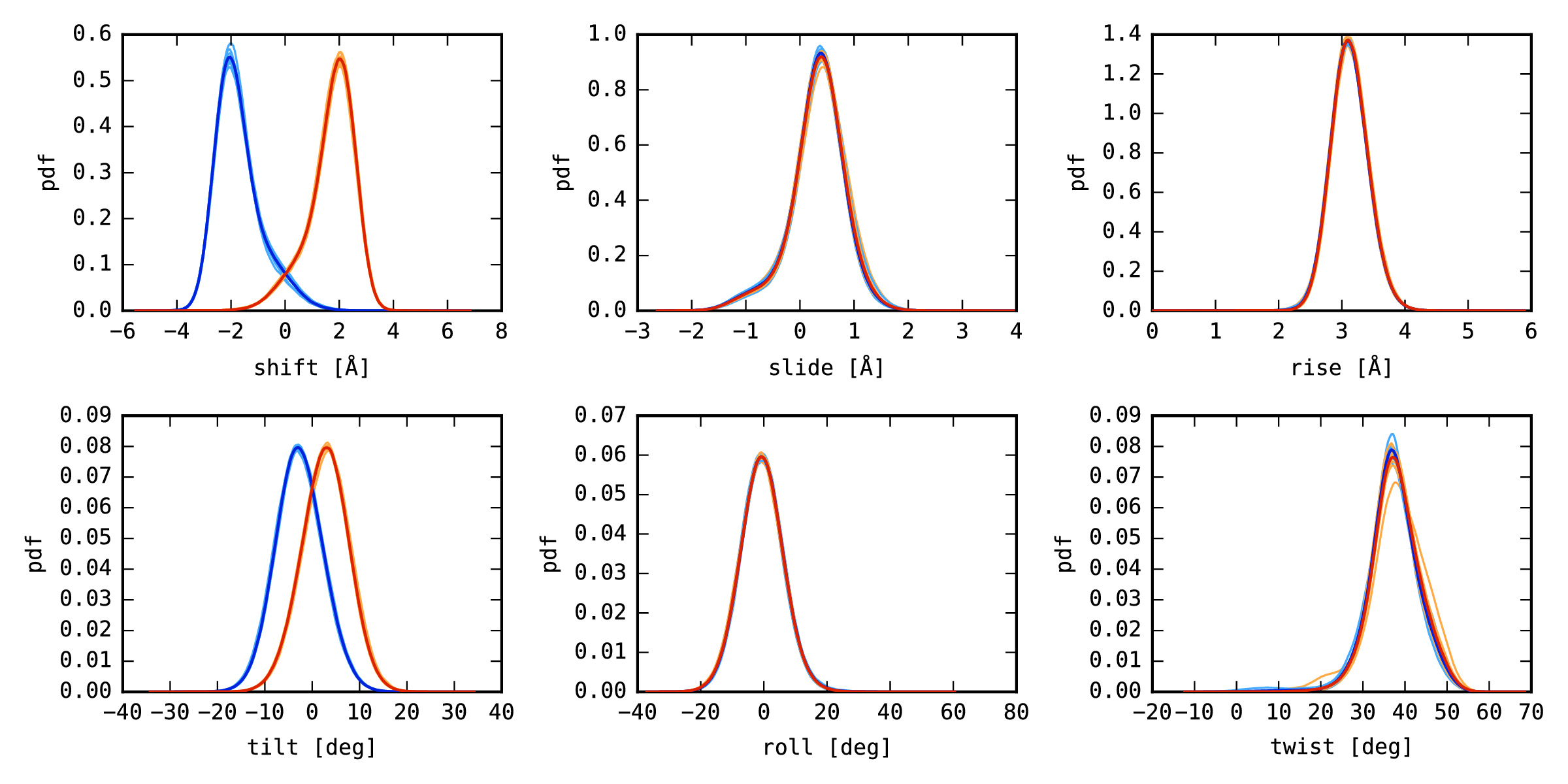
Figure S4: Probability density functions (pdf) of the parameters of the central base-pair step TA, shown for ten 510-ns-long trajectories (light blue), and for the aggregated ensemble (dark blue), where either A₄ (blue) or A₁₀ (orange) were in the cationic form.

6.4 Fitting Relaxation Data

The results of alternative fitting choices on DEGN times series are shown in Table S9 together with the final ones. Recall the fitting function:

$$f(t)=a_{1}\exp\left[-\frac{t}{t_{1}}\right]+a_{2}\exp\left[-\left(\frac{t}{t_{2}}\right)^{\!\!c_{2}}\right]+a_{3}\exp\left[-\left(\frac{t}{t_{3}}\right)^{\!\!c_{3}}\right]+a_{4}\exp\left[-\frac{t}{\tau}\right]$$ (S8)

A single exponential and a single stretched-exponential fit are shown to demonstrate that they are insufficient, and also to provide an idea of the typical magnitudes of RSS/TSS. The extremely stretched exponential ($c_{2}=0.146$) performs perhaps better than expected.

DEGN	$a_{1}$	$t_{1}$	$a_{2}$	$t_{2}$	$c_{2}$	$a_{3}$	$t_{3}$	$c_{3}$	$a_{4}$	$\tau$	RSS/TSS
Q	0.34	0.0080	0.37	0.198	0.516	0.21	1.43	0.488	0.08	654	0.0076
uncert.	0.03	0.0004	0.11	0.052	0.090	0.08	1.62	0.104	0.01	95
Q	0.23	0.0090	0.69	0.240	0.367				0.08	654	0.0082
uncert.	0.05	0.0004	0.06	0.051	0.032				0.01	91
Q			1	0.431							2.74
Q			1	0.040	0.146						0.110

Table S9: Parameters from the fitting of Eq. S8 to the data series of DEGN; $t_{i}$ in ps.

The results of alternative fitting choices on the times series of shift and tilt are shown in Table S10 together with the final ones. A four-exponential function was tested also:

$$f(t)=a_{1}\exp\left[-\frac{t}{t_{1}}\right]+a_{2}\exp\left[-\left(\frac{t}{t_{2}}\right)^{\!\!c_{2}}\right]+a_{3}\exp\left[-\frac{t}{t_{3}}\right]+a_{4}\exp\left[-\frac{t}{\tau}\right]$$ (S9)

	$a_{1}$	$t_{1}$	$a_{2}$	$t_{2}$	$c_{2}$	$a_{3}$	$t_{3}$	$a_{4}$	$\tau$	RSS/TSS
Q shift	0.27	0.281	1.28	55.5	0.568			1.89	603	0.00033
uncert.	0.02	0.078	0.30	20.1	0.071			0.33	41
Q shift	0.30	0.272	0.48	9.47	0.724	0.70	107	1.96	603	0.00027
uncert.	0.05	0.040	0.20	5.81	0.365	0.26	52	0.27	46
Q shift	0.37	4.15	0.83	85.3				1.98	603	0.00073
Q tilt	1.48	0.133	3.28	61.4	0.633			3.53	685	0.0019
uncert.	0.13	0.088	0.97	59.9	0.180			0.88	171
Q tilt	1.55	0.0896	1.15	6.66	0.629	2.15	99.6	3.65	685	0.0018
uncert.	0.23	0.0639	0.35	3.75	0.332	0.62	48.4	0.56	127
Q tilt	0.86	3.59	2.42	86.3				3.68	685	0.0030

Table S10: Parameters from the fitting of Eq. S9 to the data series of shift and tilt. $t_{i}$ in ps; $a_{i}$ in ångstrøm and degrees for shift and tilt, respectively.

Among the data series from electron transfer simulations, the fits of the shift and the tilt behave similarly, and are marginally improved upon the inclusion of a fourth exponential. On the other hand, considering the component $a_{2}$ non-stretched deteriorates the fit considerably.

6.4.1 Fitting accuracy and uncertainty

The accuracy of the obtained fits was judged by the ratio of the residual sum of squares and the total sum of squares, RSS/TSS, given as

$$\textrm{RSS/TSS}=\frac{\sum_{i}^{n}\left(y_{i}-f(x_{i})\right)^{2}}{\sum_{i}^{n}\left(y_{i}-\bar{y}\right)^{2}}$$ (S10)

for a data series $(x_{i},y_{i})$ ($i=1,\ldots{},n$) with a mean value of $\bar{y}=\sum_{i}^{n}y_{i}/n$, and a fitted function $f(x)$.

The statistical uncertainty of the parameters was estimated as follows: The entire ensemble of data series was divided into ten disjunctive groups, so that each group contained 10,000 shorter data series and 100 longer data series. Then, the data series in each of the groups were averaged to produce a single data series representative of the respective group, which was subject to fitting with the function in Eq. S8 or S9. Thus, ten values were obtained for each of the parameters of the fitting function. Finally, standard deviation was calculated for each of the parameters, from the values obtained from fitting to the ‘small’ data series. These values quantify the uncertainty of determination of that parameter. The line ‘tot’ contains the parameters obtained from fitting to the entire data series, while each numbered line contains values from a fit to a data series obtained by averaging over one tenth of the available data. The result is a sample standard deviation $\sigma(x)=\sqrt{\sum_{i}(x_{i}-\bar{x})^{2}/(n-1)}$ obtained for the ensemble of the respective parameter $x$ in the table, excluding any outlier fits, marked ‘*’; $\bar{x}$ is the average value of the parameter $x$, and $n$ is the number of non-outlier values considered.

fit	RSS/TSS	$a_{1}$	$t_{1}$	$a_{2}$	$t_{2}$	$c_{2}$	$a_{3}$	$t_{3}$	$c_{3}$	$a_{4}$	$\tau$
0	0.0109	0.38	0.0073	0.23	0.129	0.714	0.30	1.08	0.58	0.092	517
1	0.0114	0.33	0.0082	0.49	0.267	0.471	0.11	3.68	0.43	0.073	710
2	0.0111	0.34	0.0080	0.38	0.205	0.499	0.19	1.45	0.47	0.086	537
3*	0.0129	0.38	0.0080	0.07	0.124	2.683	0.45	0.58	0.49	0.092	613
4	0.0121	0.34	0.0080	0.41	0.232	0.502	0.17	1.83	0.45	0.080	691
5	0.0115	0.29	0.0086	0.57	0.281	0.429	0.06	5.89	0.33	0.071	643
6*	0.0158	0.36	0.0079	0.07	0.124	2.844	0.48	0.52	0.47	0.090	753
7	0.0105	0.34	0.0081	0.39	0.210	0.511	0.18	1.71	0.50	0.087	615
8	0.0128	0.34	0.0081	0.45	0.232	0.498	0.13	2.84	0.54	0.079	790
9	0.0129	0.30	0.0086	0.56	0.293	0.431	0.08	3.85	0.27	0.068	732
tot	0.0076	0.34	0.0080	0.37	0.198	0.516	0.21	1.43	0.49	0.083	654
$\sigma$		0.03	0.0004	0.11	0.052	0.090	0.08	1.62	0.10	0.008	95

Table S11: Electron transfer – DEGN.

fit	RSS/TSS	$a_{1}$	$t_{1}$	$a_{2}$	$t_{2}$	$c_{2}$	$a_{4}$	$\tau$
0	0.00208	0.29	0.322	1.42	61.2	0.652	1.64	637
1*	0.00326	0.28	0.300	2.83	234.8	0.582	0.34	580
2	0.00171	0.30	0.361	1.50	74.2	0.640	1.69	553
3	0.00391	0.31	0.339	0.91	32.3	0.679	2.23	645
4	0.00344	0.32	0.375	1.09	40.0	0.712	2.00	677
5*	0.00296	0.35	3.652	262.58	529.8	0.998	–259.99	531
6	0.00205	0.30	0.276	0.70	15.8	0.727	2.56	601
7	0.00207	0.32	0.378	0.79	27.7	0.775	2.30	583
8	0.00188	0.34	0.526	1.14	48.0	0.838	1.97	613
9*	0.00289	0.37	3.816	229.74	586.1	0.995	–226.90	589
tot	0.00033	0.27	0.281	1.28	55.5	0.568	1.89	603
$\sigma$		0.02	0.078	0.30	20.1	0.071	0.33	41

Table S12: Electron transfer – shift.

fit	RSS/TSS	$a_{1}$	$t_{1}$	$a_{2}$	$t_{2}$	$c_{2}$	$a_{4}$	$\tau$
0	0.0164	1.63	0.122	3.28	63.9	0.662	3.16	784
1	0.0146	1.37	0.320	4.13	104.4	0.779	2.42	998
2*	0.0126	1.61	0.125	10.14	328.4	0.607	–3.11	680
3	0.0171	1.48	0.095	2.36	27.6	0.576	4.58	642
4	0.0162	1.19	0.241	2.98	55.7	0.679	3.78	696
5	0.0154	1.43	0.069	2.72	34.8	0.422	4.11	450
6	0.0159	1.33	0.142	4.99	205.8	0.491	2.37	811
7	0.0144	1.38	0.257	1.99	29.2	0.942	4.60	545
8	0.0162	1.32	0.213	2.97	45.6	0.865	3.77	788
9*	0.0137	1.57	0.107	8.36	296.6	0.608	–1.56	639
tot	0.0019	1.48	0.133	3.28	61.4	0.633	3.53	685
$\sigma$		0.13	0.088	0.97	59.9	0.180	0.88	171

Table S13: Electron transfer – tilt.

6.5 Relaxation Plots

Figure S7: Correlation diagrams of all possible pairs of helical parameters of the central TA base-pair step with the adenine in the radical cation state. The time is color coded from blue to red.

6.6 Relaxation simulations extended to 10 ns

7 Miscellaneous

7.1 Full author list of references truncated in the main text

Ref. 51 – Case et al. is ¹⁹; Ref. 61 – Olson et al. is ¹⁸; Ref. 80 – Ivani et al. is ²⁰; Ref. 82 – Pasi et al. is ²¹.

References

- Marcus 1956 Marcus, R. A. On the theory of oxidation-reduction reactions involving electron transfer I. J. Chem. Phys. 1956, 24, 966–978
- Marcus and Sutin 1985 Marcus, R. A.; Sutin, N. Electron transfers in chemistry and biology. Biochim. Biophys. Acta Rev. Bioenergetics 1985, 811, 265–322
- Lodish \latinet al. 2012 Lodish, H.; Berk, A.; Zipursky, S. L.; Matsudaira, P.; Baltimore, D.; Darnell, J. Molecular Cell Biology; W. H. Freeman and Company: New York, USA, 2012; pp 151–159
- Burrows \latinet al. 1998 Burrows, C. J.; Perez, R. J.; Muller, J. G.; Rokita, S. E. Oxidative DNA damage mediated by metal-peptide complexes. Pure Appl. Chem. 1998, 70, 275–278
- Sinha and Häder 2002 Sinha, R. P.; Häder, D. UV-induced DNA damage and repair: a review. Photochem. Photobiol. Sci. 2002, 1, 225–236
- Hada and Georgakilas 2008 Hada, M.; Georgakilas, A. G. Formation of clustered DNA damage after high-LET irradiation: a review. J. Radiat. Res. 2008, 49, 203–210
- De Bont and Van Larebeke 2004 De Bont, R.; Van Larebeke, N. Endogenous DNA damage in humans: a review of quantitative data. Mutagenesis 2004, 19, 169–185
- Crespo-Hernández \latinet al. 2004 Crespo-Hernández, C. E.; Cohen, B.; Hare, P. M.; Kohler, B. Ultrafast excited-state dynamics in nucleic acids. Chem. Rev. 2004, 104, 1977–2020
- Pluhařová \latinet al. 2015 Pluhařová, E.; Slavíček, P.; Jungwirth, P. Modeling Photoionization of Aqueous DNA and Its Components. Acc. Chem. Res 2015, 48, 1209–1217
- Improta \latinet al. 2016 Improta, R.; Santoro, F.; Blancafort, L. Quantum mechanical studies on the photophysics and the photochemistry of nucleic acids and nucleobases. Chem. Rev. 2016, 116, 3540–3593
- Hall \latinet al. 1996 Hall, D. B.; Holmlin, R. E.; Barton, J. K. Oxidative DNA damage through long-range electron transfer. Nature 1996, 382, 731–735
- Schuster 2004 Schuster, G. B., Ed. Long-range charge transfer in DNA I & II; Top. Curr. Chem.; Springer: Heidelberg, Germany, 2004; Vol. 236 & 237
- Giese \latinet al. 2001 Giese, B.; Amaudrut, J.; Köhler, A.; Spormann, M.; Wessely, S. Direct observation of hole transfer through DNA by hopping between adenine bases and by tunnelling. Nature 2001, 412, 318–320
- Guo \latinet al. 2016 Guo, C.; Wang, K.; Zerah-Harush, E.; Hamill, J.; Wang, B.; Dubi, Y.; Xu, B. Molecular rectifier composed of DNA with high rectification ratio enabled by intercalation. Nat. Chem. 2016, 8, 484–490
- Teschome \latinet al. 2016 Teschome, B.; Facsko, S.; Schönherr, T.; Kerbusch, J.; Keller, A.; Erbe, A. Temperature-dependent charge transport through individually contacted DNA origami-based Au nanowires. Langmuir 2016, 32, 10159–10165
- Middleton \latinet al. 2009 Middleton, C. T.; de La Harpe, K.; Su, C.; Law, Y. K.; Crespo-Hernández, C. E.; Kohler, B. DNA excited-state dynamics: from single bases to the double helix. Annu. Rev. Phys. Chem. 2009, 60, 217–239
- Nordlund \latinet al. 1993 Nordlund, T. M.; Xu, D. G.; Evans, K. O. Excitation-energy transfer in DNA – Duplex melting and transfer from normal bases to 2-aminopurine. Biochemistry 1993, 32, 12090–12095
- Markovitsi \latinet al. 2007 Markovitsi, D.; Gustavsson, T.; Talbot, F. Excited states and energy transfer among DNA bases in double helices. Photochem. Photobiol. Sci. 2007, 6, 717–724
- Vayá \latinet al. 2012 Vayá, I.; Gustavsson, T.; Douki, T.; Berlin, Y.; Markovitsi, D. Electronic excitation energy transfer between nucleobases of natural DNA. J. Am. Chem. Soc. 2012, 134, 11366–11368
- Crespo-Hernández \latinet al. 2005 Crespo-Hernández, C. E.; Cohen, B.; Kohler, B. Base stacking controls excited-state dynamics in A·T DNA. Nature 2005, 436, 1141–1144
- Kwok \latinet al. 2006 Kwok, W.-M.; Ma, C.; Phillips, D. L. Femtosecond time-and wavelength-resolved fluorescence and absorption spectroscopic study of the excited states of adenosine and an adenine oligomer. J. Am. Chem. Soc. 2006, 128, 11894–11905
- Buchvarov \latinet al. 2007 Buchvarov, I.; Wang, Q.; Raytchev, M.; Trifonov, A.; Fiebig, T. Electronic energy delocalization and dissipation in single- and double-stranded DNA. Proc. Natl. Acad. Sci. USA 2007, 104, 4794–4797
- Huix-Rotllant \latinet al. 2015 Huix-Rotllant, M.; Brazard, J.; Improta, R.; Burghardt, I.; Markovitsi, D. Stabilization of mixed Frenkel-charge transfer excitons extended across both strands of guanine–cytosine DNA duplexes. J. Phys. Chem. Lett. 2015, 6, 2247–2251
- Fogarty \latinet al. 2013 Fogarty, A. C.; Duboué-Dijon, E.; Sterpone, F.; Hynes, J. T.; Laage, D. Biomolecular hydration dynamics: a jump model perspective. Chem. Soc. Rev. 2013, 42, 5672–5683
- Maroncelli and Fleming 1988 Maroncelli, M.; Fleming, G. R. Computer simulation of the dynamics of aqueous solvation. J. Chem. Phys. 1988, 89, 5044–5069
- Laage and Hynes 2006 Laage, D.; Hynes, J. T. A molecular jump mechanism of water reorientation. Science 2006, 311, 832–835
- Rey and Hynes 2015 Rey, R.; Hynes, J. T. Solvation dynamics in liquid water. 1 ultrafast energy fluxes. J. Phys. Chem. B 2015, 119, 7558–7570
- Andreatta \latinet al. 2005 Andreatta, D.; Pérez Lustres, J. L.; Kovalenko, S. A.; Ernsting, N. P.; Murphy, C. J.; Coleman, R. S.; Berg, M. A. Power-law solvation dynamics in DNA over six decades in time. J. Am. Chem. Soc. 2005, 127, 7270–7271
- Berg \latinet al. 2008 Berg, M. A.; Coleman, R. S.; Murphy, C. J. Nanoscale structure and dynamics of DNA. Phys. Chem. Chem. Phys. 2008, 10, 1229–1242
- Laage \latinet al. 2011 Laage, D.; Stirnemann, G.; Sterpone, F.; Rey, R.; Hynes, J. T. Reorientation and allied dynamics in water and aqueous solutions. Ann. Rev. Phys. Chem. 2011, 62, 395–416
- Sen \latinet al. 2009 Sen, S.; Andreatta, D.; Ponomarev, S. Y.; Beveridge, D. L.; Berg, M. A. Dynamics of water and ions near DNA: comparison of simulation to time-resolved stokes-shift experiments. J. Am. Chem. Soc. 2009, 131, 1724.–1735
- Pal \latinet al. 2003 Pal, S. K.; Zhao, L.; Zewail, A. H. Water at DNA surfaces: ultrafast dynamics in minor groove recognition. Proc. Natl. Acad. Sci. USA 2003, 100, 8113–8118
- Pal \latinet al. 2003 Pal, S. K.; Zhao, L.; Xia, T.; Zewail, A. H. Site- and sequence-selective ultrafast hydration of DNA. Proc. Natl. Acad. Sci. USA 2003, 100, 13746–13751
- Jimenez \latinet al. 1994 Jimenez, R.; Fleming, G. R.; Kumar, P. V.; Maroncelli, M. Femtosecond solvation dynamics of water. Nature 1994, 369, 471–473
- Voityuk \latinet al. 2004 Voityuk, A. A.; Siriwong, K.; Rösch, N. Environmental fluctuations facilitate electron-hole transfer from guanine to adenine in DNA stacks. Angew. Chem., Int. Ed. 2004, 43, 624–627
- Kubař and Elstner 2008 Kubař, T.; Elstner, M. What governs the charge transfer in DNA? The role of DNA conformation and environment. J. Phys. Chem. B 2008, 112, 8788–8798
- Kubař and Elstner 2010 Kubař, T.; Elstner, M. Coarse-grained time-dependent density functional simulation of charge transfer in complex systems: application to hole transfer in DNA. J. Phys. Chem. B 2010, 114, 11221–11240
- Kubař and Elstner 2013 Kubař, T.; Elstner, M. A hybrid approach to simulation of electron transfer in complex molecular systems. J. R. Soc. Interface 2013, 10, 20130415
- Pal \latinet al. 2006 Pal, S.; Maiti, P. K.; Bagchi, B.; Hynes, J. T. Multiple time scales in solvation dynamics of DNA in aqueous solution: the role of water, counterions, and cross-correlations. J. Phys. Chem. B 2006, 110, 26396–26402
- Pal \latinet al. 2006 Pal, S.; Maiti, P. K.; Bagchi, B. Exploring DNA groove water dynamics through hydrogen bond lifetime and orientational relaxation. J. Chem. Phys. 2006, 125, 234903
- Furse and Corcelli 2008 Furse, K. E.; Corcelli, S. A. The dynamics of water at DNA interfaces: computational studies of Hoechst 33258 bound to DNA. J. Am. Chem. Soc. 2008, 130, 13103–13109
- O’Neill and Barton 2004 O’Neill, M. A.; Barton, J. K. DNA charge transport: conformationally gated hopping through stacked domains. J. Am. Chem. Soc. 2004, 126, 11471–11483
- Zhang \latinet al. 2015 Zhang, Y.; Young, R. M.; Thazhathveetil, A. K.; Singh, A. P. N.; Liu, C.; Berlin, Y. A.; Grozema, F. C.; Lewis, F. D.; Ratner, M. A.; Renaud, N. \latinet al. Conformationally gated charge transfer in DNA three-way junctions. J. Phys. Chem. Lett. 2015, 6, 2434–2438
- Dickerson 1989 Dickerson, R. E. Definitions and nomenclature of nucleic acid structure parameters. J. Biomol. Struct. Dyn. 1989, 6, 627–634
- Ingrosso \latinet al. 2009 Ingrosso, F.; Rey, R.; Elsaesser, T.; Hynes, J. T. Ultrafast energy transfer from the intramolecular bending vibration to librations in liquid water. J. Phys. Chem. A 2009, 113, 6657–6665
- Petersen \latinet al. 2013 Petersen, J.; Moller, K. B.; Rey, R.; Hynes, J. T. Ultrafast Librational Relaxation of H2O in Liquid Water. J. Phys. Chem. B 2013, 117, 4541–4552
- Brinkmann and Hub 2016 Brinkmann, L. U. L.; Hub, J. S. Ultrafast anisotropic protein quake propagation after CO photodissociation in myoglobin. Proc. Natl. Acad. Sci. USA 2016, 113, 10565–10570
- Cornell \latinet al. 1995 Cornell, W. D.; Cieplak, P.; Bayly, C. I.; Gould, I. R.; Merz, K. M.; Ferguson, D. M.; Spellmeyer, D. C.; Fox, T.; Caldwell, J. W.; Kollman, P. A. A second generation force field for the simulation of proteins, nucleic acids, and organic molecules. J. Am. Chem. Soc. 1995, 117, 5179–5197
- Pérez \latinet al. 2007 Pérez, A.; Marchán, I.; Svozil, D.; Šponer, J.; Cheatham, T. E.; Laughton, C. A.; Orozco, M. Refinement of the AMBER force field for nucleic acids: Improving the description of / conformers. Biophys. J. 2007, 92, 3817–3829
- Bayly \latinet al. 1993 Bayly, C. I.; Cieplak, P.; Cornell, W. D.; Kollman, P. A. A well-behaved electrostatic potential based method using charge restraints for deriving atomic charges: The RESP model. J. Phys. Chem. 1993, 97, 10269–10280
- Case \latinet al. 2014 Case, D. A.; Babin, V.; Berryman, J. T.; Betz, R. M.; Cai, Q.; Cerutti, D. S.; Cheatham III, T. E.; Darden, T. A.; Duke, R. E.; Gohlke, H. \latinet al. AMBER 14; University of California, San Francisco, 2014; http://ambermd.org
- Ahlrichs \latinet al. 1989 Ahlrichs, R.; Bär, M.; Häser, M.; Horn, H.; Kölmel, C. Electronic structure calculations on workstation computers: the Program System Turbomole. Chem. Phys. Lett. 1989, 162, 165–169
- 53 TURBOMOLE v6.5, 2013, a development of University of Karlsruhe and Forschungszentrum Karlsruhe GmbH, 1989–2007, TURBOMOLE GmbH, since 2007; available from http://www.turbomole.com.
- Bader \latinet al. 1987 Bader, R. F.; Carroll, M. T.; Cheeseman, J. R.; Chang, C. Properties of atoms in molecules: atomic volumes. J. Am. Chem. Soc. 1987, 109, 7968–7979
- Tang \latinet al. 2009 Tang, W.; Sanville, E.; Henkelman, G. A grid-based Bader analysis algorithm without lattice bias. J. Phys.: Condens. Matter 2009, 21, 084204
- Hess 2008 Hess, B. P-LINCS: A parallel linear constraint solver for molecular simulation. J. Chem. Theory Comput. 2008, 4, 116–122
- Berendsen \latinet al. 1987 Berendsen, H.; Grigera, J.; Straatsma, T. The missing term in effective pair potentials. J. Phys. Chem. 1987, 91, 6269–6271
- Joung and Cheatham III 2008 Joung, I. S.; Cheatham III, T. E. Determination of alkali and halide monovalent ion parameters for use in explicitly solvated biomolecular simulations. J. Phys. Chem. B 2008, 112, 9020–9041
- Pronk \latinet al. 2013 Pronk, S.; Páll, S.; Schulz, R.; Larsson, P.; Bjelkmar, P.; Apostolov, R.; Shirts, M. R.; Smith, J. C.; Kasson, P. M.; van der Spoel, D. \latinet al. GROMACS 4.5: a high-throughput and highly parallel open source molecular simulation toolkit. Bioinformatics 2013, 29, 845–854
- Páll \latinet al. 2014 Páll, S.; Abraham, M. J.; Kutzner, C.; Hess, B.; Lindahl, E. Tackling exascale software challenges in molecular dynamics simulations with GROMACS. Lecture Notes in Computer Science. 2014; pp 3–27
- Olson \latinet al. 2001 Olson, W. K.; Bansal, M.; Burley, S. K.; Dickerson, R. E.; Gerstein, M.; Harvey, S. C.; Heinemann, U.; Lu, X. J.; Neidle, S.; Shakked, Z. \latinet al. A standard reference frame for the description of nucleic acid base-pair geometry. J. Mol. Biol. 2001, 313, 229–237
- Lu and Olson 2003 Lu, X.; Olson, W. K. 3DNA: a software package for the analysis, rebuilding and visualization of three‐dimensional nucleic acid structures. Nucleic Acids Res. 2003, 31, 5108–5121
- Kumar and Grubmüller 2015 Kumar, R.; Grubmüller, H. do_x3dna: a tool to analyze structural fluctuations of dsDNA or dsRNA from molecular dynamics simulations. Bioinformatics 2015, 31, 2583–2585
- Van Der Walt \latinet al. 2011 Van Der Walt, S.; Colbert, S. C.; Varoquaux, G. The NumPy array: a structure for efficient numerical computation. Comput. Sci. Eng. 2011, 13, 22–30
- Hunter 2007 Hunter, J. D. Matplotlib: a 2D graphics environment. Comput. Sci. Eng. 2007, 9, 90–95
- Dršata \latinet al. 2012 Dršata, T.; Pérez, A.; Orozco, M.; Morozov, A. V.; Šponer, J.; Lankaš, F. Structure, stiffness and substates of the Dickerson–Drew dodecamer. J. Chem. Theory Comput. 2012, 9, 707–721
- Voityuk \latinet al. 2001 Voityuk, A. A.; Siriwong, K.; Rósch, N. Charge transfer in DNA. Sensitivity of electronic couplings to conformational changes. Phys. Chem. Chem. Phys. 2001, 3, 5421–5425
- Furse and Corcelli 2010 Furse, K. E.; Corcelli, S. A. Molecular dynamics simulations of DNA solvation dynamics. J. Phys. Chem. Lett. 2010, 1, 1813–1820
- Kubař and Elstner 2009 Kubař, T.; Elstner, M. Solvent reorganization energy of hole transfer in DNA. J. Phys. Chem. B 2009, 113, 5653–5656
- Tipmanee \latinet al. 2010 Tipmanee, V.; Oberhofer, H.; Park, M.; Kim, K. S.; Blumberger, J. Prediction of reorganization free energies for biological electron transfer: a comparative study of Ru-modified cytochromes and a 4-helix bundle protein. J. Am. Chem. Soc. 2010, 132, 17032–17040
- Levenberg 1944 Levenberg, K. A Method for the solution of certain non-linear problems in least squares. Q. Appl. Math. 1944, 2, 164–168
- Marquardt 1963 Marquardt, D. W. An algorithm for least-squares estimation of nonlinear parameters. J. Soc. Ind. Appl. Math. 1963, 11, 431–441
- R Development Core Team 2008 R Development Core Team, R: A language and environment for statistical computing. R Foundation for Statistical Computing: Vienna, Austria, 2008; ISBN 3-900051-07-0
- Elzhov \latinet al. 2015 Elzhov, T. V.; Mullen, K. M.; Spiess, A.-N.; Bolker, B. minpack.lm: R interface to the Levenberg-Marquardt nonlinear least-squares algorithm found in MINPACK, plus support for bounds. 2015; R package version 1.2-0
- Brauns \latinet al. 2002 Brauns, E. B.; Madaras, M. L.; Coleman, R. S.; Murphy, C. J.; Berg, M. A. Complex local dynamics in DNA on the picosecond and nanosecond time scales. Phys. Rev. Lett. 2002, 88, 158101
- Conti \latinet al. 2010 Conti, I.; Altoè, P.; Stenta, M.; Garavelli, M.; Orlandi, G. Adenine deactivation in DNA resolved at the CASPT2//CASSCF/AMBER level. Phys. Chem. Chem. Phys. 2010, 12, 5016–5023
- Doorley \latinet al. 2013 Doorley, G. W.; Wojdyla, M.; Watson, G. W.; Towrie, M.; Parker, A. W.; Kelly, J. M.; Quinn, S. J. Tracking DNA excited states by picosecond-time-resolved infrared spectroscopy: signature band for a charge-transfer excited state in stacked adenine–thymine systems. J. Phys. Chem. Lett. 2013, 4, 2739–2744
- Conron \latinet al. 2010 Conron, S. M. M.; Thazhathveetil, A. K.; Wasielewski, M. R.; Burin, A. L.; Lewis, F. D. Direct measurement of the dynamics of hole hopping in extended DNA G-tracts: An unbiased random walk. J. Am. Chem. Soc. 2010, 132, 14388–14390
- Takada \latinet al. 2004 Takada, T.; Kawai, K.; Cai, X.; Sugimoto, A.; Fujitsuka, M.; Majima, T. Charge separation in DNA via consecutive adenine hopping. J. Am. Chem. Soc. 2004, 126, 1125–1129
- Ivani \latinet al. 2016 Ivani, I.; Dans, P. D.; Noy, A.; Pérez, A.; Faustino, I.; Hospital, A.; Walther, J.; Andrio, P.; Goñi, R.; Balaceanu, A. \latinet al. ParmBSC1: a refined force field for DNA simulations. Nat. Methods 2016, 13, 55–58
- Levy \latinet al. 1990 Levy, M. R.; Kitchen, D. B.; Blair, J. T.; Krogh-Jespersen, K. Molecular dynamics simulation of time-resolved fluorescence and nonequilibrium solvation of formaldehyde in water. J. Phys. Chem. 1990, 94, 4470–4476
- Pasi \latinet al. 2014 Pasi, M.; Maddocks, J. H.; Beveridge, D.; Bishop, T. C.; Case, D. A.; Cheatham III, T.; Dans, P. D.; Jayaram, B.; Lankaš, F.; Laughton, C. \latinet al. ABC: a systematic microsecond molecular dynamics study of tetranucleotide sequence effects in B-DNA. Nucleic Acids Res. 2014, 42, 12272–12283

References

- 1 W. D. Cornell, P. Cieplak, C. I. Bayly, I. R. Gould, K. M. Merz, D. M. Ferguson, D. C. Spellmeyer, T. Fox, J. W. Caldwell, and P. A. Kollman, “A second generation force field for the simulation of proteins, nucleic acids, and organic molecules,” J. Am. Chem. Soc., vol. 117, no. 19, pp. 5179–5197, 1995.
- 2 A. Pérez, I. Marchán, D. Svozil, J. Šponer, T. E. Cheatham, C. A. Laughton, and M. Orozco, “Refinement of the AMBER force field for nucleic acids: Improving the description of / conformers,” Biophys. J., vol. 92, no. 11, pp. 3817–3829, 2007.
- 3 F. Ryjáček, “Ambconv,” 2002. http://www.gromacs.org/Downloads/User_contributions /Other_software, last accessed on 21 June 2016.
- 4 H. Berendsen, J. Grigera, and T. Straatsma, “The missing term in effective pair potentials,” J. Phys. Chem., vol. 91, no. 24, pp. 6269–6271, 1987.
- 5 P. Mark and L. Nilsson, “Structure and dynamics of the TIP3P, SPC, and SPC/E water models at 298 K,” J. Phys. Chem. A, vol. 105, no. 43, pp. 9954–9960, 2001.
- 6 I. S. Joung and T. E. Cheatham III, “Determination of alkali and halide monovalent ion parameters for use in explicitly solvated biomolecular simulations,” J. Phys. Chem. B, vol. 112, no. 30, pp. 9020–9041, 2008.
- 7 G. Bussi, D. Donadio, and M. Parrinello, “Canonical sampling through velocity rescaling,” J. Chem. Phys., vol. 126, no. 1, p. 014101, 2007.
- 8 H. J. Berendsen, J. P. M. Postma, W. F. van Gunsteren, A. DiNola, and J. Haak, “Molecular dynamics with coupling to an external bath,” J. Chem. Phys., vol. 81, no. 8, pp. 3684–3690, 1984.
- 9 S. Nosé, “A unified formulation of the constant temperature molecular dynamics methods,” J. Chem. Phys., vol. 81, no. 1, pp. 511–519, 1984.
- 10 W. G. Hoover, “Canonical dynamics: equilibrium phase-space distributions,” Phys. Rev. A, vol. 31, no. 3, p. 1695, 1985.
- 11 M. Parrinello and A. Rahman, “Polymorphic transitions in single crystals: A new molecular dynamics method,” J. Appl. Phys., vol. 52, no. 12, pp. 7182–7190, 1981.
- 12 T. Darden, D. York, and L. Pedersen, “Particle mesh Ewald: An nlog(n) method for Ewald sums in large systems,” J. Chem. Phys., vol. 98, no. 12, pp. 10089–10092, 1993.
- 13 M. R. Shirts, D. L. Mobley, J. D. Chodera, and V. S. Pande, “Accurate and efficient corrections for missing dispersion interactions in molecular simulations,” J. Phys. Chem. B, vol. 111, no. 45, pp. 13052–13063, 2007.
- 14 B. Hess, “P-LINCS: A parallel linear constraint solver for molecular simulation,” J. Chem. Theory Comput., vol. 4, no. 1, pp. 116–122, 2008.
- 15 S. Pronk, S. Páll, R. Schulz, P. Larsson, P. Bjelkmar, R. Apostolov, M. R. Shirts, J. C. Smith, P. M. Kasson, D. van der Spoel, B. Hess, and E. Lindahl, “GROMACS 45: a high-throughput and highly parallel open source molecular simulation toolkit,” Bioinformatics, vol. 29, no. 7, pp. 845–854, 2013.
- 16 S. Páll, M. J. Abraham, C. Kutzner, B. Hess, and E. Lindahl, “Tackling exascale software challenges in molecular dynamics simulations with GROMACS,” in Lecture Notes in Computer Science (S. Markidis and E. Laure, eds.), vol. 8759 of Solving Software Challenges for Exascale, pp. 3–27, 2014.
- 17 R. E. Dickerson, “Definitions and nomenclature of nucleic acid structure parameters,” J. Biomol. Struc. Dyn., vol. 6, no. 4, pp. 627–634, 1989.
- 18 W. K. Olson, M. Bansal, S. K. Burley, R. E. Dickerson, M. Gerstein, S. C. Harvey, U. Heinemann, X. J. Lu, S. Neidle, Z. Shakked, H. Sklenar, M. Suzuki, C. S. Tung, E. Westhof, C. Wolberg, and H. M. Berman, “A standard reference frame for the description of nucleic acid base-pair geometry,” J. Mol. Biol., vol. 313, no. 1, pp. 229–237, 2001.
- 19 D. A. Case, V. Babin, J. T. Berryman, R. M. Betz, Q. Cai, D. S. Cerutti, T. E. Cheatham III, T. A. Darden, R. E. Duke, H. Gohlke, A. W. Goetz, S. Gusarov, N. Homeyer, P. Janowski, J. Kaus, I. Kolossváry, A. Kovalenko, T. S. Lee, S. LeGrand, T. Luchko, R. Luo, B. Madej, K. M. Merz Jr., F. Paesani, D. R. Roe, A. Roitberg, C. Sagui, R. Salomon-Ferrer, G. Seabra, C. L. Simmerling, W. Smith, J. Swails, R. C. Walker, J. Wang, R. M. Wolf, X. Wu, and P. A. Kollman, “Amber 14,” tech. rep., University of California, San Francisco, 2014. http://ambermd.org.
- 20 I. Ivani, P. D. Dans, A. Noy, A. Pérez, I. Faustino, A. Hospital, J. Walther, P. Andrio, R. Goñi, A. Balaceanu, G. Portella, F. Battistini, J. L. Gelpí, C. González, M. Vendruscolo, C. A. Laughton, S. A. Harris, D. A. Case, and M. Orozco, “Parmbsc1: a refined force field for DNA simulations,” Nat. Methods, vol. 13, no. 1, pp. 55–58, 2016.
- 21 M. Pasi, J. H. Maddocks, D. Beveridge, T. C. Bishop, D. A. Case, T. Cheatham III, P. D. Dans, B. Jayaram, F. Lankaš, C. Laughton, J. Mitchell, R. Osman, M. Orozco, A. Pérez, D. Petkevičiūtė, N. Špačková, J. Šponer, K. Zakrzewska, and R. Lavery, “ABC: a systematic microsecond molecular dynamics study of tetranucleotide sequence effects in B-DNA,” Nucleic Acids Res., vol. 42, no. 19, pp. 12272–12283, 2014.