On the Upper Limit of Separability

Abstract

We propose an approach to rapidly find the upper limit of separability between datasets that is directly applicable to HEP classification problems. The most common HEP classification task is to use $n$ values (variables) for an object (event) to estimate the probability that it is signal vs. background. Most techniques first use known samples to identify differences in how signal and background events are distributed throughout the $n$-dimensional variable space, then use those differences to classify events of unknown type. Qualitatively, the greater the differences, the more effectively one can classify events of unknown type. We will show that the Mutual Information (MI) between the $n$-dimensional signal-background mixed distribution and the answers for the known events, tells us the upper-limit of separation for that set of $n$ variables. We will then compare that value to the Jensen-Shannon Divergence between the output distributions from a classifier to test whether it has extracted all possible information from the input variables. We will also discuss speed improvements to a standard method for calculating MI.

Our approach will allow one to: a) quickly measure the maximum possible effectiveness of a large number of potential discriminating variables independent of any specific classification algorithm, b) identify potential discriminating variables that are redundant, and c) determine whether a classification algorithm has achieved the maximum possible separation. We test these claims first on simple distributions and then on Monte Carlo samples generated for Supersymmetry and Higgs searches. In all cases, we were able to a) predict the separation that a classification algorithm would reach, b) identify variables that carried no additional discriminating power, and c) identify whether an algorithm had reached the optimum separation. Our code is publicly available.

I Introduction

From particle physics to finance to medical diagnosis, classification problems are ubiquitous. In one of the most common HEP tasks, one seeks to place objects (events) into one of two categories ($\{\theta_{m}\}$, with $m=+1,-1$ for signal and background respectively) based on a set $\{x_{n}\}$ of $n$ measured values (variables) for each event. One often selects the variables used for classification by choosing those that each show some ability to discriminate between the two classes, i.e., a variable is used if its distribution differs between signal and background events. However, the process of choosing variables, known as feature selection, can be difficult because several variables that each individually show little difference between signal and background may, because of correlations with one another, be useful in classification when used together Guyon –Vergara .

Independent of the specific classification method, one typically begins with samples of both event types (known samples). These allow one to characterize differences in how signal and background events are distributed throughout the $n$-dimensional variable space. Once those differences are characterized, one uses the result to classify unknown events. In neural network methods, for example, one first uses the known samples to fix the parameters of the network model, and later uses that model to classify events of unknown type. Qualitatively, if an event of unknown type lies in a region of variable space that was populated more heavily with signal events than background events in the known samples, then the unknown event is more likely to be a signal event. Thus the fundamental question of signal-background separability is this: In the $n$-dimensional variable space, how different are the signal and background distributions? The extreme cases of complete separation and zero separation lead to perfect distinguishability and no distinguishability respectively. Any realistic problem will lie between these extremes.

To find a fundamental measure for the separability between datasets we begin with the following simple idea: When using $\{x_{n}\}$ to decide whether an event is signal or background, how much additional information would the answer give? Consider, for example, signal and background events where a single variable is used to discriminate between them. If there were no overlap of the signal and background distributions for the variable, then its value is as useful as the answer itself for classifying an event, and thus the answer would provide no additional information. At the other extreme, if the two classes of events overlap completely in the variable, then the answer would provide all the discriminating information and so its addition gives the maximum increase in information about the event type. One can easily extend this notion to the realistic case of partially overlapping distributions in a variable space of $n$-dimensions. Here, one would ask: If one added the answer to the n discriminating variables, how much information about the event type would one gain, or inversely, to what extent is the answer redundant? nj_maxent_poster

Concepts from information theory will allow us to quantify this. We will first review the concepts of Shannon Entropy, Cross Entropy, and the Kullback-Leibler Divergence, then discuss the Jensen-Shannon Divergence and its equivalence to mutual information (MI). We will show that JSD/MI is invariant under transformations from $n$-dimensions to 1-dimension as long as the relative signal-background density is maintained in the transformation. The Neymann-Pearson lemma will allow us to assert that any optimum classification algorithm will have this property. We will then use JSD and MI to describe a practical method for calculating a numerical limit on the separability of signal-background datasets and show the benefits of comparing it to the performance of a classifier.

We will first test these techniques on simple models with Gaussian distributions and then apply them to datasets from simulated particle physics data. Our software for computing separability limits, along with documentation to help users quickly calculate limits for their own datasets, is publicly available at https://github.com/albanyhep/JSDML.

II Shannon Entropy, Kullback-Leibler Divergence, and Jensen-Shannon Divergence

If one draws a list of values from a discrete probability distribution and then attempts to encode it efficiently, the Shannon Entropy Shannon , $H$, is the minimum number of bits per entry that will be needed for an average list. For a discrete distribution $Q$ with values $q_{1},q_{2}\dotsc q_{n}$, $H(Q)=-\sum_{i=1}^{n}P(q_{i})\log_{b}P(q_{i})$, where $P(q_{i})$ is the probability for $q_{i}$. (We will use log base 2 throughout, which gives $H$ units of bits). To achieve the encoding minimum given by $H$, one needs to assign values wisely in the encoding scheme. Values corresponding to large bins in $Q$ will appear more often in a typical list and so should be assigned to small values (fewer bits) for encoding. Conversely, values corresponding to small bins in Q will appear infrequently and so should be assigned to larger values (more bits) for encoding. Unsurprisingly, $H$ is a maximum for uniform distributions ($H=\log_{2}(n)$ for $n$ bins, which reduces to zero, as expected, for a single-bin distribution) and decreases as the distribution becomes less uniform. The cross entropy $H(P,Q)$ of two distributions $P$ and $Q$ is a closely related quantity. If one designs the most efficient encoding scheme for lists drawn from $Q$ but then uses it to encode lists drawn from $P$, the cross entropy $H(P,Q)=-\sum_{i=1}^{n}P(p_{i})\log_{2}P(q_{i})$ is the number, on average, of bits per entry needed for the encoding. Unless $P$ and $Q$ are identical, then encoding lists drawn from $P$, using the encoding scheme optimized for $Q$, will be less efficient and so will require, on average, more bits per entry. The number of extra bits per entry, on average, is $H(P,Q)-H(P)$ and is known as the Kullback-Leibler divergence Kullback_a ; Kullback_b ($D_{kl}(P||Q)$) or the relative entropy of $P$ with respect to $Q$. Relevant to our work, it is useful to note that because $H(P)$, $H(P,Q)$, and $D_{kl}$ are all simply sums over bins, the dimensionality of the distribution is irrelevant. A distribution of $n$ bins in $d$ dimensions can be rearranged into a distribution of $n$ bins in 1-dimension without changing them.

The Mutual Information (MI) between discrete random variables $X$ and $Y$, is the extent to which knowing the value of one of them reduces the uncertainty in the other. In terms of $D_{kl}$, $I(X;Y)=D_{kl}(p(x,y)||p(x)p(y))$ where $p(x,y)$ is the joint distribution of $x$ and $y$ and $p(x)$, and $p(y)$ are the marginal distributions. Thus $I(x;y)$ quantifies the relationship between $x$ and $y$ as the encoding penalty incurred by encoding samples drawn from $p(x,y)$ under the assumption that $p(x)$ and $p(y)$ are uncorrelated. MI has often been explored for feature extraction as an alternative to the correlation coefficient.

Although $D_{kl}$ is a widely used measure of dissimilarity, particularly for characterizing the change between prior and posterior distributions, a symmetric measure, Jensen-Shannon Divergence (JSD), is more useful for our application Lin . The JSD for $P$ and $Q$, normalized to equal numbers of entries, can be written in terms of $D_{kl}$ as $\text{JSD}(P||Q)=\frac{1}{2}D_{kl}(P||M)+\frac{1}{2}D_{kl}(Q||M)$, where, $M=\frac{1}{2}(P+Q)$ is the mixture distribution of $P$ and $Q$. Both JSD and $D_{kl}$ quantify the difference between $P$ and $Q$, but $\text{JSD}(P||Q)=\text{JSD}(Q||P)$ while generally $D_{kl}(P||Q)\neq D_{kl}(Q||P)$. To quantify the difference between signal and background, that symmetry is necessary. JSD can be understood through its close connection to MI. The JSD of $P$ and $Q$ is the MI between $\{x_{n}\}$ and the answer $\{\theta\}$ for $M$ ($\text{JSD}(P||Q)=I(M;\theta$)). Qualitatively, it measures the extent to which knowing $\{x_{n}\}$ for an event drawn from $M$ reduces the uncertainty in the answer $\theta$. Or equivalently, the extent to which knowing the variables makes the answer itself redundant. For completely overlapping (separate) distributions, the value of the variable(s) for a single event from $M$ gives no (complete) information about the answer. JSD ranges from 0 to 1 with 0 (1) corresponding to complete (no) overlap between $P$ and $Q$. Written in terms of Shannon entropy, $\text{JSD}(P||Q)=H(M)-\frac{1}{2}(H(P)+H(Q))$.

III JSD Invariance for an Optimum Classifier

In High Energy Physics (HEP) and elsewhere, one often performs signal-background classification by choosing a supervised learning algorithm (neural network, decision tree, support vector machine, etc.) in which one first optimizes (trains) on the known samples. One is effectively using the samples to try to recreate the pdfs that generated them. If one had those underlying pdfs, no ML algorithm would be needed. Given the $\{x_{n}\}$ for any unknown event, one would simply query the pdfs to determine the relative signal-background density for that position in variable space, which is also the relative signal-background likelihood for the event. The closer the model created by the ML algorithm is to the true pdfs, the more accurate it will be in classifying future events. With signal and background treated as two simple hypotheses, the Neyman-Pearson Lemma tells us that the likelihood ratio for the event’s point in variable space is the uniformly most powerful test for its type Neyman .

Although in the studies we report below we used neural networks as the ML algorithm, the results on separability are independent of this choice. We chose them because they are widely used in HEP and in other fields, and because excellent implementations are readily available. We used the Tensorflow implementation with Keras as a front end TensorFlow ; Keras . The networks all had an input layer with a number of nodes equal to the number of input variables ($n$), two hidden layers with varying numbers of nodes, and an output layer with a single node. This commonly used architecture results in a network that reduces the $n$-dimensional input space to a 1-dimensional output space. For a fully optimized network, the output value for an event will match the relative signal-background density for that event’s location in the original $n$-dimensional space Richard ; Zhang . If one views the input and output spaces as binned, a fully optimized network effectively collects the bins from the input space that have equal signal-background ratios and merges them into a single bin in the output space. That this transformation will leave JSD unchanged is easy to see qualitatively. Recall that JSD between the signal and background can be expressed in terms of MI as the reduction in uncertainty about the event’s type that comes from knowing the $\{x_{n}\}$, or equivalently, the event’s bin in variable space. Because that reduction in uncertainty depends only on the signal-background ratio of the bin, combining bins with the same signal-background ratio does not change MI. We show this more formally in the appendix.

IV Applying JSD and MI to measure separability and separation

An optimum algorithm will leave JSD invariant as it transforms the signal and background distributions from $n$-dimensional input to 1-dimensional output. Both JSD between the input distributions (JSD_before ) and JSD between the output distributions (JSD_after ) will be useful. JSD_before will define how much discrimination we can ever achieve with $\{x_{n}\}$, and so lets us compare different potential sets. JSD_after , when compared to JSD_before , will tell us whether or not an algorithm has extracted all possible information from the input variables it was given.

It is useful to be precise about JSD as a figure of merit (FOM). The values for $\{x_{n}\}$ that maximizes JSD_before will reduce the information contained in the signal-background answer more than the values from any other set of variables. If JSD_after =JSD_before , then the output value of the algorithm reduces the information in the answer as much as the input variables do. Maximizing this FOM does not guarantee an optimum for other FOM’s, such as $S^{2}/B$ (where $S$ and $B$ are signal and background efficiency), or the area under an accept–reject curve, or false-signal errors or false-background errors. The optimum for any of these FOM’s will generally not be the optimum for the others, and so they cannot be optimized simultaneously. Thus, careful choice of the cost function for an algorithm may still increase a particular FOM. In practice, this is often a small effect, and the set $\{x_{n}\}$ that maximizes one of them is likely able to maximize the others. Further, the requirement that JSD_after =JSD_before will still guarantee that all available information is being used.

Because the output signal and background distributions are 1-dimensional, it is straightforward to calculate JSD_after using $\text{JSD}(P||Q)=H(M)-\frac{1}{2}(H(P)+H(Q))$, where $P$ and $Q$ are the signal and background distributions, respectively. Because the input data are n-dimensional, calculating JSD_before is far more difficult. Its equivalence to MI, however, allows us to use recent advances for computing MI non-parametrically by Kraskov, Stögbauer, and Grassberger (KSG) Kraskov . Unlike kernel density approaches, KSG uses neighbor distances to estimate local density and so avoids the intermediate step of finding a pdf for the variable space. They point out that although nearest-neighbor methods have long been effective for making non-parametric estimates of entropy, one cannot calculate MI from those estimates by simply using $\text{JSD}(P||Q)=H(M)-\frac{1}{2}(H(P)+H(Q))$ because the errors on the individual entropies will not cancel. They developed a dedicated nearest neighbor method for computing MI.

The well-known estimator for relative entropy by Kozachenko-Leonenko KL is given by

$$S\approx\frac{d}{M}\sum_{i}\log(\lambda_{i})-\psi(k)+\psi(N)+\log(V_{d})$$

where d, N are the dimension and number of points in the sample space, $V_{d}$ is the volume of the unit ball of dimension $d$, $M$ is the number of mean non-vanishing distances $\lambda_{i}$ of nearest-neighbors $k$, and $\psi(k)$ is the digamma function

$$\psi(x)=\frac{\Gamma^{\prime}(x)}{\Gamma(x)}$$

where $\Gamma(x)$ is the gamma function. When $x$ is an integer we can write this as

$$\psi(n)=\sum_{k}^{n-1}\frac{1}{k}-\gamma$$

where $\gamma$ is the Euler-Mascheroni constant; $\gamma\approx 0.57721$. It has been studied extensively and works well even in high dimensions Delattre . To use it for MI however, one would need to find the differences between several entropies. KSG point out that the errors on these entropies will not necessarily cancel, and can lead to unstable or non-physical MI values. In the spirit of KL’s relative entropy estimator, KSG, developed an MI estimator given by

$$\text{MI}(x;y)\approx\psi(k)+\psi(N)-\frac{1}{k}-\langle\psi(n_{x})+\psi(n_{y})\rangle$$

where the $\psi(k)$ are still the digamma function except now one averages over the digamma functions $\psi(n_{x})$ and $\psi(n_{y})$, where $n_{x}$, $n_{y}$ are the number of nearest neighbors in the marginal spaces of $x$ and $y$ that are within the mean $k$-nearest neighbor distance in the joint space. Thus, one first constructs the joint space of $x$ and $y$ and then for each point finds the nearest-neighbor distance. Then one averages over all of the digamma evaluations for the numbers of nearest-neighbors in the marginal spaces ($x$ and $y$) that fall within those distances.

For this calculation, we use the NPEET software package (Non-Parametric Entropy Estimation Toolbox) VerSteeg ; NPEET , which includes a python implementation Python ; Numpy of the KSG method. We made one modification to its implementation. Typically MI is computed among sets of continuous variables, but here we compute it between the set $\{x_{n}\}$ and a binary answer. The problem is that when performing the neighbor count in the marginal space of the answer, the points all have values of either $+1$ (signal) or $-1$ (background). To count the neighbors, NPEET uses a KD-Tree approach, but because it is unable to find reasonable bifurcation values, it reverts to brute force and becomes very slow, even if a small amount of noise is added to the values, as suggested by KSG. However, since the marginal space only contains the answer $\theta$, we already know the number of neighbors it should find and so we modified the routine to use that number directly. The result is an algorithm that finds JSD_before very quickly. For the slowest of the studies described in later sections, we found stable values of JSD_before in $\sim 30$ seconds. This is a much faster way to measure the merit of a set $\{x_{n}\}$ than fully optimizing an ML algorithm then calculating an FOM on its output. Table 1 shows the time needed to calculate JSD_before for a range of variables and numbers of events using the Higgs simulated data sample. (Details on the sample will be discussed later.) The JSD_before values are also very stable, with a relative RMS variation of 0.4% over ten independent subsamples.

# Dimensions	# Points	JSDbefore timing [sec]
1	100,000	11$4$
1	1,000,000	1$72$
2	100,000	11$5$
2	1,000,000	1$74$
5	100,000	11$6$
5	1,000,000	1$97$
10	100,000	1$14$
10	1,000,000	$311$

Table 1: Times needed to compute JSD_before for various numbers of events and variables for the Higgs sample. JSD_before calculation times for the slowest tests described in later sections, took $\sim 30$ seconds, as stable values could be found with far fewer than 1,000,000 events. Calculations were run on a fairly generic desktop computer with a fourth-generation Intel i5 cpu and 8 Gb RAM.

Though not directly addressed in KSG, we were concerned that variables with widely different ranges of values might effectively be given different weight in the MI calculation. If, for example, one has a much larger scale than the others, its values will be more important when finding the distance to the nearest neighbor. Therefore, before computing MI, we compute for a random sample of events the RMS average distance to its nearest neighbor in each dimension. We then scale each dimension of the data to force those values to match. Note that this scaling is used only to calculate JSD_before and is independent of the scaling one typically applies to neural network input variables.

MI has been studied extensively for feature selection. For example, the “Mutual Information Feature Selection” (MIFS) algorithm by Battiti Battiti is widely used to find non-redundant variables using a greedy algorithm and pairwise computation of MI between variables. While often effective, MIFS has limitations, as pairwise variable comparisons may ignore important correlations among larger groups of variables. Further, until recent improvement in calculating MI, errors in entropy calculations could reduce its effectiveness. Work since Battiti has further improved feature selection algorithms by, for example, more efficiently choosing which MI values should be computed Kwak –Fleuret . Other recent work on feature selection has taken advantage of improvements in calculating MI in higher dimensions to directly study larger subsets of variables, and to study the MI between the variables and the class answers Bonev_b –Chow , as we do here. In this work, by modifying the MI calculation, and by showing the invariance of MI under an optimum algorithm, we are able to study its importance as a practical limit of separability. In the next section, we apply this in several cases.

V Tests

Our procedure for each of the tests below is:

1. For the input data, compute MI between the answer and the n-dimensional mixed signal-background samples (JSD_before )

2. Optimize the classification algorithm on the samples.

3. Compute JSD between the output signal and background distributions produced by the algorithm (JSD_after )

V.1 Verifying JSD Invariance

We first tested the claim that JSD separation between signal and background is unchanged by processing the events through a classification algorithm. For this test we generated Gaussian distributions in five dimensions ($P(\vec{x})=\frac{1}{{\sqrt{2\pi\sigma^{2}}}}e^{-\frac{{d^{2}}}{2\sigma^{2}}}$, where $d=\sqrt{\sum_{i=1}^{5}(x_{i}-\mu_{i})^{2}}$) for both signal and background, and varied the separation between them. The 25 signal (background) distributions each had 1000 events, $\sigma=1.0$, and $\mu_{i}$ that varied between 0.04 and 1.0 (-0.04 to -1.0) in 25 steps. Combining the samples resulted in 25 signal-background samples each with 2000 events and a distance between the signal and background means ($\Delta\mu$) that varied from 0.08 in sample 1 to 2.0 in sample 25.

For each sample, we used 1400 events as a training set to optimize a fully-connected feedforward neural network with backpropagation learning. The network had an input layer with 5 nodes, two hidden layers with 11 and 4 nodes respectively, and an output layer with one node. We trained the network for 10 epochs then used the remaining 600 events as a test set to verify that it had not been overtrained.

The critical test is whether or not JSD, as a measure of signal-background separation, remains invariant as the neural-network transforms the data from five dimensions to one dimension. For each sample we first calculated JSD for the 1400 training events in the five-dimensional variable space (JSD_before ). The mean values and errors from ten independent subsamples are shown as a dashed line in Figure 1. As expected, JSD_before increases with increasing signal-background separation. For each sample we next calculated the JSD of the network output (JSD_after ) using the 600 testing events. Using the training sample to calculate JSD_before and the testing sample to calculate JSD_after , ensures that the two sets are statistically independent. The results for JSD_after are shown as a solid line in Figure 1, where again the results are the means from ten independent subsamples. As expected, the neural-network is better able to separate the samples with larger $\Delta\mu$. The key result is the excellent agreement between JSD_before and JSD_after across the entire range of $\Delta\mu$, from nearly complete overlap to nearly complete separation. In every case, the final separation that the neural network achieves (JSD_after ) is as good, but never better, than the predicted separation from looking only at the raw data in five dimensions (JSD_before ). We also tested cases where we prevented the network from reaching optimum separation by either using too few nodes or by not allowing enough training cycles. In every case we found, JSD_after $<$JSD_before .

The results for JSD fluctuate very little between subsamples. Here, and in the studies discussed below, we find that in independent subsamples, the RMS variation for JSD_before typically corresponds to $<1\%$ and is occasionally as high as $\sim 4\%$ relative uncertainty. The variation in JSD_after is typically $3$–$5\%$; its variations are dominated by variations in how each of the neural networks converges.

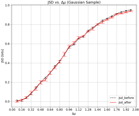
Figure 1: Comparison of JSD_before (black, dashed) to JSD_after (red, solid) for Gaussian distributions in 5-dimensions in which the signal and background separation ranges from nearly complete overlap (small $\Delta\mu$) to nearly complete separation (large $\Delta\mu$). The achieved separation by the ML algorithm (JSD_after ) tracks the predicted separation (JSD_before ) over the entire range. The results are the means from ten independent samples.

V.2 Verifying JSD Increases only When Additional Variables are Non-Redundant

Here we tested the claim that JSD is a fundamental measure of separability and hence should increase with additional discriminating variables only if they add information not already available in other variables. We generated Gaussian distributions from the same parent as in the previous study. Each signal (background) sample had 5,000 events, a mean in each dimension of 1.0 (-1.0) and a variance in each dimension of 1.0. As in the previous test, we compared JSD_before to JSD_after . Here however, we added the five discriminating variables one at a time, then compared JSD_before to JSD_after following the addition of each one. Figure 2 shows that adding additional variables increases the predicted upper limit of separation and also the separation that the neural network achieves. As in the previous test, JSD_before and JSD_after are consistent with one another (though there is some evidence that with five variables the network did not completely reach the optimum). As before, the mean values and errors are from ten independent subsamples.

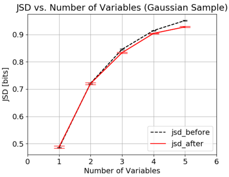
Figure 2: Comparison of JSD_before (black, dashed) to JSD_after (red, solid) for Gaussian signal and background distributions in 5-dimensions. The signal-background separation is fixed, and the five discriminating variables are added to the ML algorithm one at a time. The achieved separation by the ML algorithm (JSD_after ) improves with each additional variable, and it tracks the predicted separation (JSD_before ). The results are the means from ten independent samples.

To test our ability to identify redundant information, we repeated the above test, except that after adding the first three variables, one at a time, we added two variables that were made to be functions of the first three. Then finally we added the last two independent variables. Thus the fourth and fifth added variables contained no new information. Figure 3 shows that JSD improves as one adds information from variables 1 through 3, but then does not improve further when adding the next two. The last two variables bring JSD back up to the level it reached in the previous test. As before, JSD_before and JSD_after track each other well throughout. This ability to identify the underlying total information content available for distinguishing between the classes even in cases where variables may be functions of one another is important for feature selection. Knowing a priori the maximum possible separability allows one to judge how much information, if any, is lost when choosing a subset of all available variables for class separation. One does not need to know how variables may depend on one other to determine the maximum achievable separation between event types.

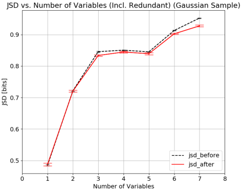
Figure 3: This figure shows the same comparison made in Figure 2, except that here, variables four and five are functions of the first three. JSD_before correctly indicates that those two variables do not increase the separability of the samples. Adding the last two independent variables (now, the sixth and seventh) brings the predicted separability back to the level seen in Figure 2. The results are the means from ten independent samples.

V.3 Simulated Data for Particle Physics Searches

To test our approach on more realistic data, we used two simulated datasets produced by Baldi, Sadowski, and Whiteson (BSW) for their study on particle physics search methods BSW . They produced two simulated (Monte Carlo) datasets that mimic information that would be available in a particle physics search at the Large Hadron Collider. Madgraph5 madgraph was used as the generator and Pythia pythia was used for hadronization and showering. The detector response was then simulated using DELPHES delphes .

One set mimics a Higgs search, and the other a Supersymmetry (SUSY) search. Both sets have kinematic variables for discriminating signal from background that are typical of those available in a Large Hadron Collider (LHC) dataset; both datasets are publicly available mlrepo . The data have “low-level” and “high-level” variables. The low-level variables are kinematic event features expected to be helpful in distinguishing signal from background. The high-level variables are functions of the low-level variables, hence they contain no new information and so in principle are extraneous. In practice, however, classifiers are often unable to extract all available information from low-level variables, and so derived quantities often improve separation performance. BSW investigated the effects of a neural-network’s architecture and learning methods on its signal-background separation performance, and also on its ability to use low-level variables without reliance on high-level variables. Below, we find that our predicted separability limits for their datasets are just above the maximum separations that our networks were ultimately able to reach. In the case of the Higgs sample, we were also able to compare our limits to the separation their network achieved, and again find that they are consistent. We also find that including or excluding the high-level variables has no effect on our limit, verifying the important principle that it is a limit on fundamental signal-background separability, unaffected by redundant information.

V.3.1 Higgs Sample

For signal events in the Higgs sample, a theoretical neutral Higgs boson is produced through the fusion of two gluons. The neutral Higgs decays into a charged Higgs and a $W$ boson. The charged Higgs then decays into a $W$ and the Standard-Model (SM) Higgs. This SM Higgs then decays predominantly into charged $b$ quarks. The products are thus a pair of charged $W$’s and a pair of charged $b$ quarks which further decay or hadronize respectively. The process for the background events also produces a pair of charged W’s and a pair of b quarks, but without the intermediate Higgs state. This leads to kinematic differences that can be used for signal-background discrimination. The events are described by 21 low-level and 7 high-level variables. Because several of the low-level variables are discrete, and the Kraskov estimator for mutual information is designed for continuous variables, we decided for this study to make comparisons only with the high-level variables. (We expect that it will be straightforward to modify the algorithms to work with both continuous and discrete input.) Because the difference between signal and background events is the presence or absence of intermediate Higgs particles, all seven of the high-level variables are mass estimates made by combining the individual observed particles from the $W$ decays and the groups of particles, known as jets, produced by the $b$ quarks.

We divided a 5-million-event sample into 10 equal subsets. As in the previous test, we tracked the separability limit as we added high-level variables one at a time. After each was added, we optimized a neural network and measured the separation it achieved. The networks, had an input layer with a number of nodes equal to the number of input variables, two hidden layers with 34 and 27 nodes, and an output layer with one node. We trained the networks for 1000 epochs using, 70% of the sample for training and 30% for testing. Our optimized networks approached but never surpassed the predicted separability limit (see Figure 4).

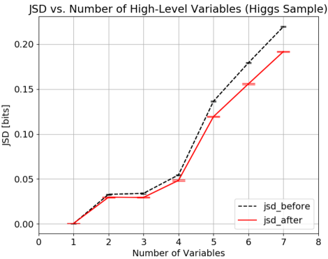
Figure 4: Comparison of JSD_before (black, dashed) to JSD_after (red, solid) for the Higgs sample as high-level discriminating variables are added one at a time. JSD_before increases as each of the seven high-level variables is added. The achieved separation by the ML algorithm (JSD_after ) tracks the predicted separation (JSD_before ) reasonably throughout, without ever exceeding the predicted separations. The results are the means from ten independent samples.

We also used the performance of the networks in BSW as a benchmark. BSW converted the output distributions of their networks into background rejection vs. signal efficiency curves, commonly known as Receiver Operating Characteristic (ROC) curves. They then used the total area under the ROC curve (AUC) as their figure of merit. Larger values of AUC correspond to better signal-background separation. We compared the AUC values from our networks to those in BSW to ensure that we were using their data correctly, and also to verify that our networks were reasonably well optimized, as they took extensive efforts to verify that their networks had converged fully. As expected, in the cases where their networks were significantly larger, they reached slightly higher AUC values (see Table 2).

We next attempted to compare their achieved separation to our separability limit. To do this, we used the bin-values from their ROC curves to reconstruct network output distributions, which then allowed us to compute the JSD_after FOM for their networks. They first tested a small network that they noted did not achieve a high-level of discrimination. We estimate that its output corresponds to a separation of JSD_after =0.15 , which is less than our predicted limit of JSD_before =0.22. They then used a much larger network and we found that its output corresponds to a separation of JSD_after =0.22. The key point is that their large well-optimized network reaches but does not surpass the separability limit that we predicted from the raw data. The full results are shown in Table 2.

	High-level vars only
JSDbefore (this work)	0.22 (0.001)
JSDafter (this work)	0.19 (0.002)
JSDafter (BSW, shallow network)	0.15
JSDafter (BSW, deep network)	0.22
AUC (this work)	0.78
AUC (BSW, shallow network)	0.78
AUC (BSW, deep network)	0.80

Table 2: Comparison of JSD and AUC values for the 7 high-level variables in the Higgs sample. Lines two and three show that neither of the two smaller networks (ours or the shallow network in BSW) reach the predicted separation (line one). The larger network in BSW (line four) reaches but does not surpass the prediction. The last three lines show AUC values that we used to verify our networks against those in BSW. Lines one, two, and five are the means from ten independent samples and the values in parentheses are the RMS variations among them.

V.3.2 Supersymmetric (SUSY) Sample

For the SUSY sample, the signal events are a process in which supersymmetric $\chi^{\pm}$ particles are produced and then decay to $W$ bosons and a supersymmetric $\chi^{0}$. The $W$’s subsequently decay to charged leptons and neutrinos. The $\chi^{0}$ and the neutrinos are not directly observable and their presence is inferred from momentum imbalance and missing energy in the detector. The background events are from a Standard Model process in which two $W$ bosons are produced and each decays to a charged lepton and a neutrino. The signal and background events can be distinguished because they differ in the number of invisible particles and in the kinematics of the decays. The events are described by eight low-level variables: For each of the two leptons, its angle is described by two variables and its momentum transverse to the beamline by one variable. Two additional low-level variables give the energy and momentum imbalance caused by the undetected particles. There are ten high-level variables derived from these eight. The details of these are unimportant for our studies because, as functions of the eight low-level variables, they contain no additional information.

We divided the 5-million-event sample into 10 equal subsets and optimized neural networks on the low-level variables, the high-level variables, and both low-level and high-level combined (all). The networks had two hidden layers with 24 nodes and 17 nodes respectively and a single output node. As required, we adjusted the number of input nodes to match the number of input variables. We trained the networks for 100 epochs using, as before, 70% of the sample for training and 30% for testing.

As in the Higgs study, to ensure that our networks were well optimized, we compared the AUC values to those in BSW . Figure 5 shows the AUC performance of the networks on low-only, high-only, and all variables. Table 3 compares these AUC values to the networks from BSW.

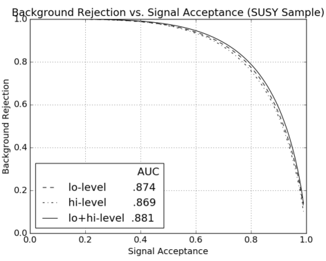
Figure 5: Neural network background rejection vs. signal acceptance ROC curves for the SUSY sample. The low-level only, high-level only, and low+high-level sets are shown as dashed, dot-dashed, and solid curves respectively. The ROC curves from our networks were used to verify the reasonableness of our networks against those in BSW. The AUC results from these curves also appear in Table 3

We next made the key comparison of JSD_before to JSD_after . Table 3 shows the results for networks trained on the 8 low-level variables, the 10 high-level variables, and all 18 variables. For all three cases JSD_after approaches, but never surpasses JSD_before .

	Low only	High only	Both
JSDbefore (this work)	0.36 (0.002)	0.36 (0.002)	0.37 (0.002)
JSDafter (this work)	0.35 (0.004)	0.35 (0.005)	0.36 (0.005)
AUC (this work)	0.87	0.87	0.88
AUC (BSW, shallow network)	0.86	0.86	0.88
AUC (BSW, deep network)	0.88	0.87	0.88

Table 3: Comparison of JSD and AUC values for the SUSY sample. The top line shows the JSD_before values for the 8 low-level, the 10 high-level, and the 18 combined variable sets. Line two shows that our neural network separation reaches but does not surpass the predicted separability. The last three lines show AUC values that we used to verify our networks against those in BSW. Lines one through three are the means from ten independent samples and the values in parentheses are the RMS variations among them.

Figure 6 shows the results of a separate test on this dataset in which we added variables one at a time, and compared JSD_before to JSD_after following the addition of each. As in the second test with Gaussians, the predicted separation and achieved separation agree, and both continue to improve as each additional low-level variable is included. Importantly, JSD_before and JSD_after both stop increasing once all the low-level variables have been included. High-level variables (derived quantities) do not change the fundamental separability of the datasets.

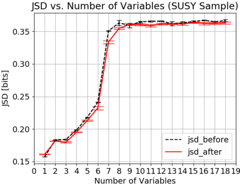
Figure 6: Comparison of JSD_before (black, dashed) to JSD_after (red, solid) for the SUSY sample as discriminating variables are added one at a time. JSD_before increases as each of the eight low-level variables is added. It does not increase further as the ten high-level variables are included. This is expected because the high-level variables do not bring additional discriminating information. The achieved separation by the ML algorithm (JSD_after ) tracks the predicted separation (JSD_before ) throughout. The results are the means from ten independent samples.

VI Conclusion

Distinguishing signal from background based on a set of descriptive quantities, is an important task in a wide range of fields. We have proposed that using known samples, one can place a limit on the separability between two event types by finding the Mutual Information between the known answer and all discriminating variables. Equivalent to the Jensen-Shannon Divergence, this limit is independent of the algorithm chosen to classify the events and is only reachable if the algorithm preserves the relative signal-background probability when transforming the data from the n-dimensional input space to the 1-dimensional output space. We tested these limits on two datasets of Gaussian distributions and then on two Monte Carlo samples generated to study classification algorithms in particle physics searches.

This approach has substantial practical benefits for classification problems both for feature selection and for algorithm evaluation. One benefit for feature selection is that one can take a large number of potential variables and quickly determine the separability that could be reached if all of them were used at once. With that benchmark in hand, one can then monitor the separability that would be lost by using any subset of the variables. Feature selection also benefits because once a set is selected, one can quickly investigate any potential new variables that might be added. The separability limit will increase if the new variables bring new information but not if they are effectively functions of those already being used. The benefits to algorithm choice and optimization are clear. There are dozens of approaches to classification tasks, and sub-methods for most of them. By comparing the separation achieved by a given method to the separability limit calculated on the input data, one knows whether or not the method has achieved the best possible separation. In short, you know when you’re done.

Our software for computing separability limits, along with documentation to help users quickly calculate limits for their own datasets, is publicly available at https://github.com/albanyhep/JSDML.

VII Acknowledgments

We thank Arial Caticha, Eric Dohner, Adam Fischer, Philip Goyal, Vivek Jain, Kevin Knuth, Oleg Lunin, Udo von Toussant, Kevin Vanslette, Greg Ver Steeg, and Daniel Whiteson for helpful discussions.

VIII References

IX Appendix

IX.1 Proof of the Data Processing Inequality

Starting from the discussion in Cover and Thomas CoverThomas , here we give a concise proof of the data processing inequality in terms of Mutual Information, which for $y=f(\{x\})$, and two categories of events $\theta=\{+1,-1\}$, states that $\mathcal{M}[\theta;x]\geq\mathcal{M}[\theta;y]$. This enforces the idea that a transformation y=f({x}) of the input variables can not increase their ability to distinguish between the classes. Given variables $\theta$,$x$,$y$ which form a Markov chain

$$\theta\rightarrow x\rightarrow y$$ (1)

implies the joint probability can be written

$$p(\theta,x,y)=p(\theta)p(x|\theta)p(y|x)$$ (2)

where $p(y|x)$ is independent of $\theta$. We can appeal to the symmetric nature of the mutual information to break it up in two different ways

$$\mathcal{M}[\theta;x,y] =\mathcal{M}[\theta;x]+\mathcal{M}[\theta;y|x]$$

$$=\mathcal{M}[\theta;y]+\mathcal{M}[\theta;x|y]$$ (3)

but because of the Markov property that $p(y|x,\theta)=p(y|x)$, we have that $\mathcal{M}[\theta;y|x]=0$. And since mutual information is always positive, $\mathcal{M}[\theta;x,y]\geq 0$ we conclude

$$\mathcal{M}[\theta;x]\geq\mathcal{M}[\theta;y]$$ (4)

with equality only when $\mathcal{M}[\theta;x|y]=0$ or when $y$ is a sufficient statistic for $x$

$$p(\theta|x)=p(\theta|y)\qquad\mathrm{i.e.}\qquad\theta\rightarrow y\rightarrow x$$ (5)

References

- (1) I. Guyon, An Introduction to Variable and Feature Selection, Journal of Machine Learning Research 3, 1157-1182,(2003).
- (2) B. Bonev, F. Escolano, M. Cazorla, Feature selection, mutual information, and the classification of high-dimensional patterns, Pattern Analysis and Applications”, 3, 309-319, (2008).
- (3) J. Vergara, P. Estévez, A Review of Feature Selection Methods Based on Mutual Information, Neural Computing & Applications, 24, 1, 175-186, (2014).
- (4) N. Carrara, E. Dohner, J. Ernst, Estimating an Upper Bound on Class Discrimination with the Jensen-Shannon Divergence, Poster, 36th International Workshop on Bayesian Inference and Maximum Entropy Methods in Science and Engineering. July 10-15, 2016, Ghent, Belgium.
- (5) Shannon, Claude E. A Mathematical Theory of Communication, Bell System Technical Journal. 27 (3): 379–423, (1948)
- (6) Kullback, S., Leibler, R.A., On information and sufficiency, Annals of Mathematical Statistics. 22 (1): 79–86, (1951).
- (7) Kullback, S., Information Theory and Statistics. John Wiley & Sons, (1959).
- (8) Lin, J., Divergence measures based on the shannon entropy, IEEE Transactions on Information Theory, 37 (1): 145–151, 1991.
- (9) J. Neyman, E. Pearson, On the Problem of the Most Efficient Tests of Statistical Hypotheses. Philosophical Transactions of the Royal Society A: Mathematical, Physical and Engineering Sciences. 231, 694–706, (1933).
- (10) Google Research, TensorFlow: Large-Scale Machine Learning on Heterogeneous Systems, http://tensorflow.org/, 2015.
- (11) F. Chollet, Keras, GitHub, https://github.com/fchollet/keras, 2015.
- (12) M. Richard, R. Lippmann, Neural network classifiers estimate Bayesian a posteriori probabilities, Neural Comput., 3, 461–483, (1991).
- (13) G. Zhang, Neural Networks for Classification: A Survey, IEEE Transactions on Systems, Man, and Cybernetics—Part C: Applications and Reviews, 30, 4, (2000)
- (14) A. Kraskov, H. Stögbauer, P. Grassberger, Estimating mutual information, Phys. Rev. E 69, 066138, (2004).
- (15) L.F. Kozachenko, N.N. Leonenko, A statistical estimate for the entropy of a random vector, Problemy Peredachi Informatsii 23, 9–16, (1987).
- (16) S. Delattre, N. Fournier, On the Kozachenko-Leonenko entropy estimator, arXiv:1602.07440, (2016)
- (17) G. Ver Steeg, A. Galstyan, Information-Theoretic Measures of Influence Based on Content Dynamics, arXiv:1208.4475 (2012)
- (18) G. Ver Steeg, NPEET: Nonparamateric entropy estimation toolbox, https://github.com/gregversteeg/NPEET (2015)
- (19) G. van Rossum, Python tutorial, Technical Report CS-R9526, Centrum voor Wiskunde en Informatica (CWI), Amsterdam, May 1995.
- (20) SciPy Developers, NumPy, https://github.com/numpy/numpy.git, 2017.
- (21) R. Battiti, Using mutual information for selecting features in supervised neural net learning, IEEE Trans. Neural Netw., vol. 5, no.4, 1994.
- (22) N. Kwak and C.H. Choi, Input feature selection for classification problems, IEEE Trans. Neural Netw., vol. 3, no.1, 2002.
- (23) H. Peng, F. Long and C. Ding, Feature selection based on mutual information: Criteria of max-dependency, max-relevance and min-redundancy, IEEE Trans. Pattern Anal. Mach. Intell. vol. 27, no.8, 2005.
- (24) K.E. Hild, D. Erdogmus, K. Torkkola and J.C. Principe, Feature extraction using information theoretic learning, IEEE Trans. Pattern Anal. Mach. Intell., vol. 28, no.9, 2006.
- (25) V. Sindhwani, S. Rakshit, D. Deodhar, D. Erdogmus, J. Principe and P. Niyogi, Feature selection in MLPs and SVMs based on maximum output information, IEEE Trans. Neural Netw., vol. 15, no.4, 2004.
- (26) P. Estévez, Normalized Mutual Information Feature Selection, IEEE Trans. Neural Netw., vol. 20, no.2, 2009.
- (27) S. Foithong, O. Pinngern and B. Attachoo, Feature subset selection wrapper based on mutual information and rough sets, Expert Systems with Applications 39, 2012.
- (28) F. Fleuret, Fast Binary Feature Selection with Conditional Mutual Information, Journal of Machine Learning Research 5 (2004)
- (29) B. Bonev, F. Escolano, M. Cazorla Feature selection, mutual information, and the classification of high-dimensional patterns, Pattern Analysis and Applications, 11:309–319, (2008)
- (30) K. Torkkola, Feature Extraction by Non-Parametric Mutual Information Maximization, Journal of Machine Learning Research 3, 1415-1438, (2003)
- (31) T. W. Chow and D. Huang, Estimating optimal feature subsets using efficient estimation of high-dimensional mutual information, IEEE Trans. Neural Netw., vol. 16, no.1, 2005.
- (32) Baldi, P., P. Sadowski, and D. Whiteson, Searching for Exotic Particles in High-energy Physics with Deep Learning, Nature Communications 5 (July 2, 2014).
- (33) Alwall, J. et al. MadGraph 5 : Going Beyond. JHEP 1106, 128 (2011).
- (34) Sjostrand, T. et al. PYTHIA 6.4 physics and manual. JHEP 05, 026 (2006).
- (35) Ovyn, S., Rouby, X. & Lemaitre, V. DELPHES, a framework for fast simulation of a generic collider experiment (2009).
- (36) UCI Machine Learning Repository, Lichman, M. http://archive.ics.uci.edu/ml
- (37) T.M. Cover, J.A. Thomas, Elements of Information Theory, Wiley, New York, 1991.