A Probabilistic proof of the breakdown of Besov regularity in $L$-shaped domains

Abstract

We provide a probabilistic approach in order to investigate the smoothness of the solution to the Poisson and Dirichlet problems in $L$-shaped domains. In particular, we obtain (probabilistic) integral representations (9), (12)–(14) for the solution. We also recover Grisvard’s classic result on the angle-dependent breakdown of the regularity of the solution measured in a Besov scale.
Key Words. Brownian Motion; Dirichlet Problem; Poisson Equation; Conformal Mapping; Stochastic Representation; Besov Regularity.
MSC 2010. 60J65; 35C15; 35J05; 35J25; 46E35.

1 Introduction

Let us consider the (homogeneous) Dirichlet problem

$$\operatorname{\varDelta}f =0 \text{in $G$},$$ (1)

$$f|_{\partial G} =h \text{on $\partial G$},$$

where $G\subset\mathbb{R}^{d}$ is a domain with Lipschitz boundary $\partial G$ and $\operatorname{\varDelta}$ denotes the Laplace operator, i.e. $\operatorname{\varDelta}=\sum_{i=1}^{d}\frac{\partial^{2}}{\partial x_{i}^{2}}$. In order to show that there exists a solution to (1) which belongs to some subspace of $L_{p}(G)$, say, to the Besov space $B_{pp}^{\sigma}(G)$, $\sigma>0$, it is necessary that $h$ is an element of the trace space of $B_{pp}^{\sigma}(G)$ on $\partial G$; it is well known that the trace space is given by $B_{pp}^{\sigma-1/p}(\partial G)$, see Jerison & Kenig (JK95, , Theorem 3.1), a more general version can be found in Jonsson & Wallin (JW84, , Chapter VII), and for domains with $C^{\infty}$-boundary a good reference is Triebel (Tr83, , Sections 3.3.3–4). The smoothness of the solution $f$, expressed by the parameter $\sigma$ in $B_{pp}^{\sigma}(G)$, is, however, not only determined by the smoothness of $h$, but also by the geometry of $G$. It seems that Grisvard Gr85 is the first author to quantify this in the case when $G$ is a non-convex polygon. Subsequently, partly due to its relevance in scientific computing, this problem attracted a lot of attention; for instance, it was studied by Jerison & Kenig JK95 , by Dahlke & DeVore DD97 in connection with wavelet representations of Besov functions, by Mitrea & Mitrea MM03 and Mitrea, Mitrea & Yan MMY10 in Hölder spaces, to mention but a few references.

In this note we use a probabilistic approach to the problem and we obtain a probabilistic interpretation in the special case when $G$ is an $L$-shaped domain of the form $\mathbb{L}:=\mathbb{R}^{2}\backslash\{(x,y):\,x,y\geq 0\}$, see Figure 1, and in an $L_{2}$-setting.

[scale=0.8]domain-l

Figure 1: The $L$-shaped model domain $\mathbb{L}\subset\mathbb{R}^{2}$.

This is the model problem for all non-convex domains with an obtuse interior angle. In this case the Besov space $B_{22}^{\sigma}(\mathbb{L})$ coincides with the Sobolev–Slobodetskij space $W_{2}^{\sigma}(\mathbb{L})$. In particular, we

• give a probabilistic interpretation of the solution to (1) with $G=\mathbb{L}$;

• provide a different proof of the fact that the critical order of smoothness of $f$ is $\sigma<\pi/\frac{3\pi}{2}=\frac{2}{3}$, i.e.´ even for $h\in C_{0}^{2}(\partial\mathbb{L})$ we may have

  $$f\in W_{2,\mathrm{loc}}^{1+\sigma}(\mathbb{L}),\quad\sigma<\tfrac{2}{3},\qquad\text{and}\qquad f\notin W_{2}^{1+\sigma}(\mathbb{L}),\quad\sigma\geq\tfrac{2}{3};$$ (2)

• apply the “breakdown of regularity” result to the Poisson (or inhomogeneous Dirichlet) problem.

It is clear that this result holds in a more general setting, if we replace the obtuse angle $3\pi/2$ by some $\theta\in(\pi,2\pi)$.

Results of this type were proved for polygons and in a Hölder space setting by Mitrea & Mitrea MM03 . Technically, our proof is close (but different) to that given in MM03 —yet our staring idea is different. Dahlke & DeVore DD97 proved this regularity result analytically using a wavelet basis for $L_{p}$-Besov spaces.

Problem (1) is closely related to the Poisson (or nonhomogeneous Dirichlet) problem

$$\operatorname{\varDelta}F =g \text{on $G$},$$ (3)

$$F|_{\partial G} =0 \text{on $\partial G$}.$$

If $G$ is bounded and has a $C^{\infty}$-boundary, the problems (1) and (3) are equivalent. Indeed, in this case for every right-hand side $g\in L_{2}(G)$ of (3) there exists a unique solution $F\in W_{2}^{2}(G)$, see Triebel (Tr83, , Theorem 4.3.3). Denote by $N$ the Newtonian potential on $\mathbb{R}^{d}$ and define $w:=g*N$; clearly, $\operatorname{\varDelta}w=g$ on $G$ and $w\in W_{2}^{2}(G)$. Since the boundary is smooth, there is a continuous linear trace operator $\operatorname{Tr}:W_{2}^{2}(G)\to W_{p}^{3/2}(\partial G)$ as well as a continuous linear extension operator $\operatorname{Ex}:W_{2}^{3/2}(\partial G)\to W_{2}^{2}(G)$, such that $\operatorname{Tr}\circ\operatorname{Ex}=\operatorname{id}$, cf. Triebel Tr83 . Hence, the function $f:=w-F$ solves the inhomogeneous Dirichlet problem (1) with $h=\operatorname{Tr}w$ on $\partial G$. On the other hand, let $f$ be the (unique) solution to (1). Since there exists a continuous linear extension operator from $W_{2}^{3/2}(\partial G)$ to $W_{2}^{2}(G)$ given by $\tilde{h}=\operatorname{Ex}h$, we see that the function $F:=f-\tilde{h}$ satisfies (3) with $g=\operatorname{\varDelta}\tilde{h}$.

If the boundary $\partial G$ is Lipschitz the situation is different. It is known, see for example Jerison & Kenig (JK95, , Theorem B)) that, in general, on a Lipschitz domain $G$ and for $g\in L_{2}(G)$ one can only expect that the solution $F$ to (3) belongs to $W_{2}^{3/2}(G)$; there are counterexamples of domains, for which $F$ cannot be in $W_{2}^{\alpha}(G)$ for any $\alpha>3/2$. Thus, the above procedure does not work in a straightforward way. However, by our strategy we can recover the negative result for this concrete domain, cf. Theorem 2.2: If $g\in H_{1}(\mathbb{R}^{2})\cap W_{2}^{1}(\mathbb{L})$, then the solution $F$ to (3) is not in $W_{2}^{1+\sigma}(\mathbb{L})$ for any $\sigma\geq 2/3$. Here $H_{1}(\mathbb{R}^{2})\subset L_{1}(\mathbb{R}^{2})$ is the Hardy space, cf. Stein stein .

If $G$ is unbounded, the solution to (1) might be not unique and, in general, it is only in the local space $W^{2}_{2,\mathrm{loc}}(G)$ even if $\partial G$ is smooth, cf. Gilbarg & Trudinger (gil-tru, , Chapter 8). On the other hand, if the complement $G^{c}$ is non-empty, if no component of $G^{c}$ reduces to a single point, and if the boundary value $h$ is bounded and continuous on $\partial G$, then there exists a unique bounded solution to (1) given by the convolution with the Poisson kernel, see Port & Stone (PS78, , Theorem IV.2.13).

A strong motivation for this type of results comes from numerical analysis and approximation theory, because the exact Besov smoothness of $u$ is very important for computing $u$ and the feasibility of adaptive computational schemes, see Dahlke & DeVore DD97 , Dahlke, Dahmen & DeVore DDD97 , DeVore De98 , Cohen, Dahmen & DeVore CDD01 , Cohen C03 ; an application to SPDEs is in Cioika et. al. Ci11 ; Ci14 . More precisely—using the set-up and the notation of CDD01 —let $\{\psi_{\lambda},\,\lambda\in\Lambda\}$ be a basis of wavelets on $G$ and assume that the index set $\Lambda$ is of the form $\Lambda=\bigcup_{i\geq 0}\Lambda_{i}$ with (usually hierarchical) sets $\Lambda_{i}$ of cardinality $N_{i}$. By $u_{\Lambda_{i}}$ we denote the Galerkin approximation of $u$ in terms of the wavelets $\{\psi_{\lambda}\}_{\lambda\in\Lambda_{i}}$ (this amounts to solving a system of linear equations), and by $e_{N_{i}}(u):=\|u-u_{\Lambda_{i}}\|_{p}$ the approximation error in this scheme. Then it is known, cf. (CDD01, , (4.2) and (2.35)), that

$$u\in W_{p}^{\sigma}(G)\implies e_{N_{i}}(u)\leq CN_{i}^{-\sigma/d},\quad i\geq 1.$$ (4)

There is also an adaptive algorithm for choosing the index sets $(\Lambda_{i})_{i\geq 1}$. Starting with an initial set $\Lambda_{0}$, this algorithm adaptively generates a sequence of nested sets $(\Lambda_{i})_{i\geq 1}$; roughly speaking, in each iteration step we choose the next set $\Lambda_{i+1}$ by partitioning the domain of those wavelets $\psi_{\lambda}$, $\lambda\in\Lambda_{i}$ (i.e. selectively refining the approximation by considering the next generation of wavelets), whose coefficients $u_{\lambda}$ make, in an appropriate sense, the largest contribution to the sum $u=\sum_{\lambda\in\Lambda_{i}}u_{\lambda}\psi_{\lambda}$.

Notation. Most of our notation is standard. By $(r,\theta)\in(0,\infty)\times(0,2\pi]$ we denote polar coordinates in $\mathbb{R}^{2}$, and $\mathbb{H}$ is the lower half-plane in $\mathbb{R}^{2}$. We write $f\asymp g$ to say that $cf(t)\leq g(t)\leq Cf(t)$ for all $t$ and some fixed constants.

2 Setting and the main result

Let $B=(B_{t}^{x})_{t\geq 0}$ be a Brownian motion started at a point $x\in G$. Suppose that there exists a conformal mapping $\varphi:G\to\mathbb{H}$, where $\mathbb{H}:=\{(x_{1},x_{2})\in\mathbb{R}^{2},\,\,x_{2}\leq 0\}$ is the lower half-plane in $\mathbb{R}^{2}$. Using the conformal invariance of Brownian motion, see e.g. Mörters & Peres (MP10, , p. 202), we can describe the distribution of the Brownian motion inside $G$ in terms of some Brownian motion $W$ in $\mathbb{H}$, which is much easier to handle. Conformal invariance of Brownian motion means that there exists a planar Brownian motion $W=(W_{t}^{y})_{t\geq 0}$ with starting point $y\in\mathbb{H}$ such that, under the conformal map $\varphi:G\to\mathbb{H}$ with boundary identification,

$$\left(\varphi(B_{t}^{x})\right)_{0\leq t\leq\tau_{G}}\quad\text{has the same law as}\quad\left(W_{\xi(t)}^{\varphi(x)}\right)_{0\leq t\leq\tau_{\mathbb{H}}};$$ (5)

the time-change $\xi$ is given by $\xi(t):=\int_{0}^{t}|\varphi^{\prime}(B^{x}_{s})|^{2}\,{\mathrm{d}}s$; in particular, $\xi(\tau_{G})=\tau_{\mathbb{H}}$, where $\tau_{G}=\inf\{t>0:B_{t}^{x}\in\partial G\}$ and $\tau_{\mathbb{H}}:=\inf\{t>0:\,W_{t}^{\varphi(x)}\in\partial\mathbb{H}\}$ are the first exit times from $G$ and $\mathbb{H}$, respectively.

Let us recall some properties of a planar Brownian motion in $\mathbb{H}$ killed upon exiting at the boundary $\partial\mathbb{H}=\{(w_{1},w_{2}):\,w_{2}=0\}$. The distribution of the exit position $W_{\tau_{\mathbb{H}}}$ has the transition probability density

$$u\mapsto p_{\mathbb{H}}(w,u)=\frac{1}{\pi}\frac{|w_{2}|}{|u-w_{1}|^{2}+w_{2}^{2}},\quad w=(w_{1},w_{2})\in\mathbb{H},$$ (6)

cf. Bass (Bass, , p. 91). Recall that a random variable $X$ with values in $\mathbb{R}$ has a Cauchy distribution, $X\sim\mathsf{C}(m,b)$, $m\in\mathbb{R}$, $b>0$, if it has a transition probability density of the form

$$p(u)=\frac{1}{\pi}\frac{b}{(u-m)^{2}+b^{2}},\quad u\in\mathbb{R};$$

if $X\sim\mathsf{C}(m,b)$, then $Z:=(X-m)/b\sim\mathsf{C}(0,1)$. Thus, the probabilistic interpretation of $W_{\tau_{\mathbb{H}}}^{w}$ is

$$W_{\tau_{\mathbb{H}}}^{w}\sim Z^{w}\sim\mathsf{C}(w_{1},|w_{2}|)\quad\text{or}\quad W_{\tau_{\mathbb{H}}}^{w}\sim\frac{Z-w_{1}}{|w_{2}|}\quad\text{where}\quad Z\sim\mathsf{C}(0,1).$$ (7)

This observation allows us to simplify the calculation of functionals $\Theta$ of a Brownian motion $B$ on $G$, killed upon exiting from $G$, in the following sense:

$$\mathbb{E}\Theta(B_{\tau_{G}}^{x})=\mathbb{E}\left(\Theta\circ\varphi^{-1}\right)(\varphi(B_{\tau_{G}}^{x})) =\mathbb{E}\left(\Theta\circ\varphi^{-1}\right)(W_{\tau_{\mathbb{H}}}^{\varphi(x)})$$ (8)

$$=\mathbb{E}\left(\Theta\circ\varphi^{-1}\right)\left(\frac{Z-\varphi_{1}(x)}{|\varphi_{2}(x)|}\right).$$

In particular, the formula (8) provides us with a probabilistic representation for the solution $f$ to the Dirichlet problem (1):

$$f(x)=\mathbb{E}h(B_{\tau_{G}}^{x})=\mathbb{E}\left(h\circ\varphi^{-1}\right)(W_{\tau_{\mathbb{H}}}^{\varphi(x)}).$$ (9)

Remark 1

The formulae in (8) are very helpful for the numerical calculation of the values $\mathbb{E}\Theta(B_{\tau_{G}}^{x})$. In fact, in order to simulate $\Theta(B_{\tau_{G}}^{x})$, it is enough to simulate the Cauchy distribution $Z\sim\mathsf{C}(0,1)$ and then evaluate (8) using the Monte Carlo method.

We will now consider the $L$-shaped domain $\mathbb{L}$. It is easy to see that the conformal mapping of $\mathbb{L}$ to $\mathbb{H}$ is given by

$$\varphi(z)=\mathrm{e}^{{\rm i}\frac{2\pi}{3}}z^{2/3}=r^{2/3}\exp\left(\tfrac{2}{3}{\rm i}(\theta+\pi)\right)=\varphi_{1}(r,\theta)+{\rm i}\varphi_{2}(r,\theta),$$ (10)

cf. Figure 2, where $\theta=\arg z\in(0,2\pi]$.

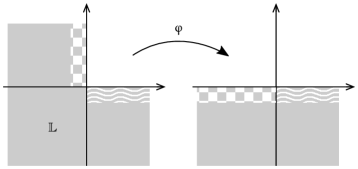
Figure 2: Conformal mapping from $\mathbb{L}$ to $\mathbb{H}$ and its behaviour at the boundaries.

The following lemma uses the conformal mapping $\varphi:\mathbb{L}\to\mathbb{H}$ and the conformal invariance of Brownian motion to obtain the distribution of $B^{x}_{\tau_{\mathbb{L}}}$.

Lemma 1

Let $\mathbb{L}$ be an $L$-shaped domain as shown in Fig. 1. The exit position $B_{\tau_{\mathbb{L}}}$ of Brownian motion from $\mathbb{L}$ is a random variable on $\partial\mathbb{L}=\{0\}\times[0,\infty)\cup[0,\infty)\times\{0\}$ which has the following probability distribution:

$$\mathbb{P}\left(B^{x}_{\tau_{\mathbb{L}}}\in{\mathrm{d}}y\right) =\frac{1}{\pi}\frac{|\varphi_{2}(x)|}{|\varphi_{1}(x)+y_{2}|^{2}+|\varphi_{2}(x)|^{2}}\,{\mathrm{d}}y_{2}\,\delta_{0}({\mathrm{d}}y_{1})$$ (11)

$$\qquad\mbox{}+\frac{1}{\pi}\frac{|\varphi_{2}(x)|}{|\varphi_{1}(x)-y_{1}|^{2}+|\varphi_{2}(x)|^{2}}\,{\mathrm{d}}y_{1}\,\delta_{0}({\mathrm{d}}y_{2}).$$

Lemma 1 provides us with an explicit representation of the solution $f(x)$ to the Dirichlet problem (1) for $G=\mathbb{L}$. Indeed, since (cf. Figure 2)

$$\left(h\circ\varphi^{-1}\right)(u)=\begin{cases}h(u,0),&u\geq 0,\\ h(0,-u),&u\leq 0,\end{cases}$$

we get

$$f(x)=\int_{\mathbb{R}}f_{0}(u)\,p_{\mathbb{H}}(\varphi(x),u)\,{\mathrm{d}}u=\frac{1}{\pi}\int_{\mathbb{R}}f_{0}(u)\,\frac{|\varphi_{2}(x)|}{(\varphi_{1}(x)-u)^{2}+|\varphi_{2}(x)|^{2}}\,{\mathrm{d}}u,$$ (12)

where

$$f_{0}(u):=h(0,-u)\mathds{1}_{(-\infty,0)}(u)+h(u,0)\mathds{1}_{[0,\infty)}(u).$$ (13)

After a change of variables, this becomes

$$f(x)=\frac{1}{\pi}\int_{\mathbb{R}}f_{0}\left(u|\varphi_{2}(x)|+\varphi_{1}(x)\right)\frac{{\mathrm{d}}u}{u^{2}+1}.$$ (14)

If we want to investigate the smoothness of $f$, it is more convenient to rewrite $f$ in polar coordinates. From the right-hand side of (10) we infer

$$\varphi_{1}(r,\theta)=r^{2/3}\cos\Phi_{\theta}\quad\text{and}\quad\varphi_{2}(r,\theta)=r^{2/3}\sin\Phi_{\theta},$$ (15)

where we use the shorthand

$$\Phi_{\theta}:=\frac{2}{3}(\pi+\theta).$$

Observe that for $\theta\in(\pi/2,2\pi]$ we have $\pi<\Phi_{\theta}\leq 2\pi$, hence $\varphi_{2}\leq 0$. This yields

$$f(r,\theta)=\frac{1}{\pi}\int_{\mathbb{R}}f_{0}\left(r^{2/3}\cos\Phi_{\theta}-r^{2/3}v\sin\Phi_{\theta}\right)\,\frac{{\mathrm{d}}v}{1+v^{2}}.$$ (16)

Now we turn to the principal objective of this note: the smoothness of $f$ in the Sobolev–Slobodetskij scale.

Theorem 2.1

Consider the (homogeneous) Dirichlet problem (1) with a boundary term $f_{0}$, given by (17), and let $f$ denote the solution to (1).

1. If $f_{0}\in W_{1}^{2}(\mathbb{R})\cap W_{2}^{2}(\mathbb{R})$ satisfies

   $$\liminf_{\epsilon\to 0}\int_{|x|>\epsilon}\frac{f_{0}^{\prime}(x)}{x}\,{\mathrm{d}}x\neq 0,$$ (17)

   then $f\notin W_{2}^{1+\sigma}(\mathbb{L})$, even $f\notin W_{2,\mathrm{loc}}^{1+\sigma}(\mathbb{L})$, for any $\sigma\geq 2/3$.

2. If $f_{0}\in W_{1}^{2}(\mathbb{R})\cap W_{p}^{1}(\mathbb{R})$, where $p>\max\{2,\,2/(2-3\sigma)\}$, then $f\in W_{2,\mathrm{loc}}^{1+\sigma}(\mathbb{L})$ for all $\sigma\in(0,2/3)$.

Remark 2

By the Sobolev embedding theorem we have $W_{1}^{2}(\mathbb{R})\cap W_{2}^{2}(\mathbb{R})\subset C_{b}(\mathbb{R})$ and $W_{1}^{2}(\mathbb{R})\cap W_{p}^{1}(\mathbb{R})\subset C_{b}(\mathbb{R})$ if $p>\max\{2,\,2/(2-3\sigma)\}$. Hence, the function $f$ given by (14) is the unique bounded solution to (1).

The idea of the proof of Theorem 2.1 makes essential use of the results by Jerison & Kenig JK95 combined with the observation that it is, in fact, enough to show the claim for $\widehat{\mathbb{L}}:=\mathbb{L}\cap B(0,1)$, where $B(0,1):=\{x\in\mathbb{R}^{2}:\,|x|<1\}$.

Theorem 2.1 allows us to prove the negative result for the solution to the Poisson problem, which improves (JK95, , Theorem B). Recall that $H_{1}(\mathbb{R}^{2})\subset L_{1}(\mathbb{R}^{2})$ is the usual Hardy space, cf. Stein stein .

Theorem 2.2

Consider the Poisson (inhomogeneous Dirichlet) problem (3) with right-hand side $g\in H_{1}(\mathbb{R}^{2})\cap W_{2}^{1}(\mathbb{L})$ such that $f_{0}(x):=\left((\operatorname{Tr}g*N)\circ\varphi^{-1}\right)(x)$ satisfies (17), where $N(x)=(2\pi)^{-1}\log|x|$ is the Newton kernel. Then the solution $F\notin W_{2}^{1+\sigma}(\mathbb{L})$, even $F\notin W_{2,\mathrm{loc}}^{1+\sigma}(\mathbb{L})$, for any $\sigma\geq 2/3$.

The proofs of Theorem 2.1 and 2.2 are deferred to the next section.

3 Proofs

Proof (Proof of Lemma 1)

We calculate the characteristic function of $B^{x}_{\tau_{\mathbb{L}}}$. As before, let $y=(y_{1},y_{2})$, $x=(x_{1},x_{2})$ and $\varphi(x)=(\varphi_{1}(x),\varphi_{2}(x))$. We have

$$\mathbb{E}\mathrm{e}^{{\rm i}\xi\cdot B_{\tau_{\mathbb{L}}}^{x}} \overset{\eqref{BW1}}{=}\mathbb{E}\mathrm{e}^{{\rm i}\xi\cdot\varphi^{-1}(W_{\tau_{\mathbb{H}}}^{\varphi(x)})}$$

$$=\int_{\mathbb{R}^{2}}\mathrm{e}^{{\rm i}\xi\cdot\varphi^{-1}(y)}\,\mathbb{P}(W_{\tau_{\mathbb{H}}}^{\varphi(x)}\in{\mathrm{d}}y)$$

$$\overset{\eqref{WH}}{=}\frac{1}{\pi}\int_{\mathbb{R}}\mathrm{e}^{{\rm i}\xi\cdot\varphi^{-1}(y_{1},0)}\frac{|\varphi_{2}(x)|}{|\varphi_{1}(x)-y_{1}|^{2}+|\varphi_{2}(x)|^{2}}{\mathrm{d}}y_{1}$$

$$=\frac{1}{\pi}\int_{-\infty}^{0}\mathrm{e}^{-{\rm i}\xi_{2}u}\frac{|\varphi_{2}(x)|}{|\varphi_{1}(x)-u|^{2}+|\varphi_{2}(x)|^{2}}\,{\mathrm{d}}u$$

$$\qquad\mbox{}+\frac{1}{\pi}\int_{0}^{+\infty}\mathrm{e}^{{\rm i}\xi_{1}u}\frac{|\varphi_{2}(x)|}{|\varphi_{1}(x)-u|^{2}+|\varphi_{2}(x)|^{2}}\,{\mathrm{d}}u.$$ ∎

For the proof of Theorem 2.1 we need some preparations. In order to keep the presentation self-contained, we quote the classical result by Jerison & Kenig (JK95, , Theorem 4.1).

Theorem 3.1 (Jerison & Kenig)

Let $\sigma\in(0,1)$, $k\in\mathbb{N}_{0}$ and $p\in[1,\infty]$. For any function $u$ which is harmonic on a bounded domain $\Omega$, the following assertions are equivalent:

1. $f\in B_{pp}^{k+\sigma}(\Omega)$;

2. $\operatorname{\operatorname{dist}}(x,\partial\Omega)^{1-\sigma}\,\left|\nabla^{k+1}f\right|+\left|\nabla^{k}f\right|+\left|f\right|\in L_{p}(\Omega)$.

We will also need the following technical lemma. Recall that $\widehat{\mathbb{L}}=\mathbb{L}\cap B(0,1)$.

Lemma 2

Suppose that $f_{0}\in W_{p}^{1}(\mathbb{R})$ for some $p>2$. Then $f\in W_{2}^{1}(\widehat{\mathbb{L}})$.

Proof

Using the representation (16), the Hölder inequality and a change of variables, we get

$$\int_{\pi/2}^{2\pi}\int_{0}^{1}|f(r,\theta)|^{2}r\,{\mathrm{d}}r\,{\mathrm{d}}\theta$$

$$=\frac{3}{2\pi^{2}}\int_{\pi/2}^{2\pi}\int_{0}^{1}\rho^{2}\left|\int_{\mathbb{R}}f_{0}(w)\frac{|\rho\sin\Phi_{\theta}|}{(w-\rho\cos\Phi_{\theta})^{2}+(\rho\sin\Phi_{\theta})^{2}}{\mathrm{d}}w\right|^{2}\,{\mathrm{d}}\rho\,{\mathrm{d}}\theta$$

$$\leq C_{1}\int_{\pi/2}^{2\pi}\int_{0}^{1}\rho^{2}\left[\left(\int_{\mathbb{R}}\left|f_{0}(v)\right|^{p}{\mathrm{d}}v\right)^{1/p}\left(\int_{\mathbb{R}}\frac{|\rho\sin\Phi_{\theta}|^{q}}{(v^{2}+|\rho\sin\Phi_{\theta}|^{2})^{q}}{\mathrm{d}}v\right)^{1/q}\right]^{2}\,{\mathrm{d}}\rho\,{\mathrm{d}}\theta$$

$$\leq C_{2}\int_{\pi/2}^{2\pi}\int_{0}^{1}\rho^{2}\left|\rho\sin\Phi_{\theta}\right|^{-2+2/q}\left(\int_{\mathbb{R}}\frac{1}{(w^{2}+1)^{q}}{\mathrm{d}}w\right)^{2/q}\,{\mathrm{d}}\rho\,{\mathrm{d}}\theta$$

$$=C_{3}\int_{\pi/2}^{2\pi}\int_{0}^{1}\rho^{2/q}\left|\sin\Phi_{\theta}\right|^{-2+2/q}\,{\mathrm{d}}\rho\,{\mathrm{d}}\theta,$$

where $p^{-1}+q^{-1}=1$. Because of $p>2$ we have $-2+2/q>-1$, hence $q<2$. Note that the inequalities $2x/\pi\leq\sin x\leq x$ for $x\in[0,\pi/2]$, imply

$$\int_{\pi/2}^{2\pi}\left|\sin\Phi_{\theta}\right|^{-1+\epsilon}\,{\mathrm{d}}\theta=\int_{0}^{\pi}\left|\sin\varphi\right|^{-1+\epsilon}\,{\mathrm{d}}\varphi=2\int_{0}^{\pi/2}\left|\sin\varphi\right|^{-1+\epsilon}\,{\mathrm{d}}\varphi<\infty.$$

This shows that $f\in L_{2}(\widehat{\mathbb{L}})$.

Recall that the partial derivatives of the polar coordinates are

$$\frac{\partial}{\partial x_{1}}r=\cos\theta,\quad\frac{\partial}{\partial x_{1}}\theta=-\frac{\sin\theta}{r},\quad\frac{\partial}{\partial x_{1}}\Phi_{\theta}=\frac{2}{3}\frac{\partial}{\partial x_{1}}\theta=-\frac{2\sin\theta}{3r}.$$ (18)

Therefore, we have for $\theta\in(\pi/2,2\pi)$

$$\frac{\partial}{\partial x_{1}} f(r,\theta)=\frac{1}{\pi}\int_{\mathbb{R}}f_{0}^{\prime}\left(r^{2/3}\cos\Phi_{\theta}-vr^{2/3}\sin\Phi_{\theta}\right)\,\frac{1}{v^{2}+1}\times$$

$$\quad\mbox{}\times\left[\frac{2\cos\theta}{3r^{1/3}}\left(\cos\Phi_{\theta}-v\sin\Phi_{\theta}\right)\right.$$

$$\quad\qquad\left.\mbox{}+r^{2/3}\left(\frac{-2\sin\theta}{3r}\right)(-v\cos\Phi_{\theta}-\sin\Phi_{\theta})\right]{\mathrm{d}}v$$ (19)

$$=\frac{2}{3\pi r^{1/3}}\int_{\mathbb{R}}f_{0}^{\prime}\left(r^{2/3}\cos\Phi_{\theta}-vr^{2/3}\sin\Phi_{\theta}\right)\,\frac{1}{v^{2}+1}\times$$

$$\quad\mbox{}\times\left[\left(\cos\Phi_{\theta}-v\sin\Phi_{\theta}\right)\cos\theta+(v\cos\Phi_{\theta}+\sin\Phi_{\theta})\sin\theta\right]{\mathrm{d}}v$$

$$=\frac{2}{3\pi r^{1/3}}\int_{\mathbb{R}}f_{0}^{\prime}\left(r^{2/3}\cos\Phi_{\theta}-vr^{2/3}\sin\Phi_{\theta}\right)\,\frac{K(\theta,v)}{v^{2}+1}\,{\mathrm{d}}v,$$

where

$$K(\theta,v):=\cos\omega_{\theta}-v\sin\omega_{\theta},$$ (20)

and

$$\omega_{\theta}=\frac{1}{3}\left(2\pi-\theta\right).$$ (21)

Note that $\Phi_{\pi/2}=\pi$ and $\omega_{\pi/2}=\pi/2$.

Let us show that the first partial derivatives of $f$ belong to $L_{2}(\widehat{\mathbb{L}})$. Because of the symmetry of $\widehat{\mathbb{L}}$, is it enough to check this for $\frac{\partial}{\partial x_{1}}f$.

Using the estimate $|K(\theta,v)|(1+v^{2})^{-1}\leq C(1+|v|)^{-1}$, a change of variables and the Hölder inequality, we get

$$\int_{0}^{1} \int_{\pi/2}^{2\pi}\left|\frac{\partial}{\partial x_{1}}f(r,\theta)\right|^{2}r\,{\mathrm{d}}\theta\,{\mathrm{d}}r$$

$$=\int_{0}^{1}\int_{\pi/2}^{2\pi}\left|\int_{\mathbb{R}}\frac{2}{3\pi r^{1/3}}\,f_{0}^{\prime}\left(r^{2/3}\cos\Phi_{\theta}-vr^{2/3}\sin\Phi_{\theta}\right)\frac{K(\theta,v)}{1+v^{2}}\,{\mathrm{d}}v\right|^{2}r\,{\mathrm{d}}\theta\,{\mathrm{d}}r$$

$$=\frac{2}{3\pi^{2}}\int_{0}^{1}\int_{\pi/2}^{2\pi}\rho\left|\int_{\mathbb{R}}f_{0}^{\prime}\left(\rho\cos\Phi_{\theta}-v\rho\sin\Phi_{\theta}\right)\frac{K(\theta,v)}{1+v^{2}}\,{\mathrm{d}}v\right|^{2}\,{\mathrm{d}}\theta\,{\mathrm{d}}\rho$$

$$\leq C_{1}\int_{0}^{1}\int_{\pi/2}^{2\pi}\rho\left(\int_{\mathbb{R}}\frac{|f_{0}^{\prime}(w)|}{|\rho\sin\Phi_{\theta}|+|w-\rho\cos\Phi_{\theta}|}{\mathrm{d}}w\right)^{2}\,{\mathrm{d}}\theta\,{\mathrm{d}}\rho$$

$$\leq C_{2}\left(\int_{\mathbb{R}}\left|f_{0}^{\prime}(w)\right|^{p}{\mathrm{d}}w\right)^{2/p}\left(\int_{\mathbb{R}}\frac{1}{(1+|w|)^{q}}{\mathrm{d}}w\right)^{2/q}\times$$

$$\qquad\mbox{}\times\int_{\pi/2}^{2\pi}\int_{0}^{1}\rho\left(|\rho\sin\Phi_{\theta}|^{-1+1/q}\right)^{2}\,{\mathrm{d}}\rho\,{\mathrm{d}}\theta$$

$$=C_{3}\int_{\pi/2}^{2\pi}\int_{0}^{1}|\sin\Phi_{\theta}|^{-2+2/q}\rho^{-1+2/q}\,{\mathrm{d}}\rho\,{\mathrm{d}}\theta<\infty;$$

in the last line we use again that $-2+2/q>-1$. ∎∎

Proof (Proof of Theorem 2.1)

It is enough to consider the set $\widehat{\mathbb{L}}$. We verify that condition b of Theorem 3.1 holds true. We check whether

$$\operatorname{\operatorname{dist}}(0,\cdot)^{1-\sigma}\left|\frac{\partial^{2}}{\partial x_{1}^{2}}f\right|+\left|\frac{\partial}{\partial x_{1}}f\right|+\left|f\right|\quad\text{is in $L_{2}(\widehat{\mathbb{L}})$ or not.}$$

From Lemma 2 we already know that $\left|\frac{\partial}{\partial x_{1}}f\right|+\left|f\right|\in L_{2}(\widehat{\mathbb{L}})$. Let us check when

$$\operatorname{\operatorname{dist}}(0,\cdot)^{1-\sigma}\left|\frac{\partial^{2}}{\partial x_{1}^{2}}f\right|\in L_{2}(\widehat{\mathbb{L}}).$$

We will only work out the term $\frac{\partial^{2}}{\partial x_{1}^{2}}f(r,\theta)$ since the calculations for $\tfrac{\partial^{2}}{\partial x_{1}\partial x_{2}}f(r,\theta)$ are similar. We have

$$\frac{\partial}{\partial x_{1}}K(\theta,v)=\frac{\sin\theta}{3r}\left(-v\cos\omega_{\theta}-\sin\omega_{\theta}\right)=:\frac{\sin\theta}{3r}K^{\star}(\theta,v),$$

where use that $\tfrac{\partial}{\partial x_{1}}\omega_{\theta}=-\frac{1}{3}\tfrac{\partial}{\partial x_{1}}\theta=\frac{\sin\theta}{3r}$ and set

$$K^{\star}(\theta,v):=-v\cos\omega_{\theta}-\sin\omega_{\theta}.$$ (22)

Therefore, differentiating $\tfrac{\partial}{\partial x_{1}}f$—we use the representation (19)—with respect to $x_{1}$ gives

$$\tfrac{\partial^{2}}{\partial x_{1}^{2}}f(r,\theta) =-\frac{2\cos\theta}{9\pi r^{4/3}}\int_{\mathbb{R}}f_{0}^{\prime}\left(r^{2/3}(\cos\Phi_{\theta}-v\sin\Phi_{\theta})\right)\frac{K(\theta,v)}{1+v^{2}}\,{\mathrm{d}}v$$

$$\qquad\mbox{}+\frac{4}{9\pi r^{2/3}}\int_{\mathbb{R}}f_{0}^{\prime\prime}\left(r^{2/3}(\cos\Phi_{\theta}-v\sin\Phi_{\theta})\right)\frac{K^{2}(\theta,v)}{1+v^{2}}\,{\mathrm{d}}v$$

$$\qquad\mbox{}+\frac{2\sin\theta}{9\pi r^{4/3}}\int_{\mathbb{R}}f_{0}^{\prime}\left(r^{2/3}(\cos\Phi_{\theta}-v\sin\Phi_{\theta})\right)\frac{K^{\star}(\theta,v)}{1+v^{2}}\,{\mathrm{d}}v.$$

Note that

$$\int_{\widehat{\mathbb{L}}}\operatorname{\operatorname{dist}}(x,\partial\widehat{\mathbb{L}})^{2-2\sigma}\left|\frac{\partial^{2}}{\partial x_{1}^{2}}f(x)\right|^{2}\,{\mathrm{d}}x$$ (23)

$$\qquad=\int_{0}^{1}\int_{\pi/2}^{2\pi}\operatorname{\operatorname{dist}}((r,\theta),\partial\widehat{\mathbb{L}})^{2-2\sigma}\left|\frac{\partial^{2}}{\partial x_{1}^{2}}f(r,\theta)\right|^{2}r\,{\mathrm{d}}\theta\,{\mathrm{d}}r.$$

Since only the values near the boundary $\Gamma:=\partial\widehat{\mathbb{L}}\cap\partial\mathbb{L}$ determine the convergence of the integral, it is enough to check that

$$\mathbb{I}=\int_{0}^{1}\int_{\pi/2}^{2\pi}\operatorname{\operatorname{dist}}((r,\theta),\Gamma)^{2-2\sigma}\left|\frac{\partial^{2}}{\partial x_{1}^{2}}f(r,\theta)\right|^{2}r\,{\mathrm{d}}\theta\,{\mathrm{d}}r$$ (24)

is infinite if $\sigma\geq 2/3$ and finite if $\sigma<2/3$.

We split $\widehat{\mathbb{L}}$ into three parts. For $\delta>0$ small enough we define, see Figure 3,

[scale=0.8]k-sets

Figure 3: The set $\widehat{\mathbb{L}}$ is split into three disjoint parts $K_{1}$, $K_{2}$, $K_{3}$.

$$K_{1}:=\left\{(r,\theta):\,0<r<1,\;\;\frac{\pi}{2}+\delta<\theta<2\pi-\delta\right\},$$

$$K_{2}:=\left\{(r,\theta):\,0<r<1,\;\;\frac{\pi}{2}\leq\theta<\frac{\pi}{2}+\delta\right\},$$

$$K_{3}:=\left\{(r,\theta):\,0<r<1,\;\;2\pi-\delta<\theta\leq 2\pi\right\}.$$

Splitting the integral accordingly, we get

$$\mathbb{I}=\left(\int_{K_{1}}+\int_{K_{2}}+\int_{K_{3}}\right)\operatorname{\operatorname{dist}}((r,\theta),\Gamma)^{2-2\sigma}\left|\frac{\partial^{2}}{\partial x_{1}^{2}}f(r,\theta)\right|^{2}r\,{\mathrm{d}}\theta\,{\mathrm{d}}r;$$

in order to show that $\mathbb{I}$ is infinite if $\sigma\geq 2/3$, it is enough to see that the integral over $K_{1}$ is infinite. Noting that in $K_{1}$ we have $\operatorname{\operatorname{dist}}((r,\theta),\Gamma)\asymp r$, we get

$$\int_{K_{1}} \left|r^{1-\sigma}\tfrac{\partial^{2}}{\partial x_{1}^{2}}f(r,\theta)\right|^{2}r\,{\mathrm{d}}\theta\,{\mathrm{d}}r$$ (25)

$$=\int_{K_{1}}r\left|r^{1-\sigma}\frac{2}{9\pi r^{4/3}}\right|^{2}\times$$

$$\quad\mbox{}\times\left|\int_{\mathbb{R}}f_{0}^{\prime}\left(r^{2/3}(\cos\Phi_{\theta}-v\sin\Phi_{\theta})\right)\frac{K^{\star}(\theta,v)\sin\theta-K(\theta,v)\cos\theta}{1+v^{2}}\,{\mathrm{d}}v\right.$$

$$\qquad\left.\mbox{}+2r^{2/3}\int_{\mathbb{R}}f_{0}^{\prime\prime}\left(r^{2/3}(\cos\Phi_{\theta}-v\sin\Phi_{\theta})\right)\frac{K^{2}(\theta,v)}{1+v^{2}}\,{\mathrm{d}}v\right|^{2}\,{\mathrm{d}}r\,{\mathrm{d}}\theta$$

$$=\frac{4}{81\pi^{2}}\int_{K_{1}}r^{1/3-2\sigma}\left|\int_{\mathbb{R}}f_{0}^{\prime}\left(r^{2/3}(\cos\Phi_{\theta}-v\sin\Phi_{\theta})\right)\frac{K^{\star\star}(\theta,v)}{1+v^{2}}\,{\mathrm{d}}v\right.$$

$$\qquad\left.\mbox{}+2r^{2/3}\int_{\mathbb{R}}f_{0}^{\prime\prime}\left(r^{2/3}(\cos\Phi_{\theta}-v\sin\Phi_{\theta})\right)\frac{K^{2}(\theta,v)}{1+v^{2}}\,{\mathrm{d}}v\right|^{2}\,{\mathrm{d}}r\,{\mathrm{d}}\theta$$

$$=\frac{4}{81\pi^{2}}\int_{K_{1}}r^{1/3-2\sigma}\left|J(r^{2/3},\theta)+I(r^{2/3},\theta)\right|^{2}\,{\mathrm{d}}r\,{\mathrm{d}}\theta$$

$$=\frac{2}{27\pi^{2}}\int_{K_{1}}\rho^{1-3\sigma}\left|J(\rho,\theta)+I(\rho,\theta)\right|^{2}\,{\mathrm{d}}\rho\,{\mathrm{d}}\theta,$$

where we use the following shorthand notation

$$K^{\star\star}(\theta,v):=K^{\star}(\theta,v)\sin\theta-K(\theta,v)\cos\theta=-v\sin(\theta-\omega_{\theta})-\cos(\theta-\omega_{\theta}),$$

$$J(\rho,\theta):=\int_{\mathbb{R}}f_{0}^{\prime}\left(\rho(\cos\Phi_{\theta}-v\sin\Phi_{\theta})\right)\frac{K^{\star\star}(\theta,v)}{1+v^{2}}\,{\mathrm{d}}v,$$

$$I(\rho,\theta):=2\rho\int_{\mathbb{R}}f_{0}^{\prime\prime}\left(\rho(\cos\Phi_{\theta}-v\sin\Phi_{\theta})\right)\frac{K^{2}(\theta,v)}{1+v^{2}}\,{\mathrm{d}}v.$$

Observe that $\theta-\omega_{\theta}\in(0,2\pi)$ for $\theta\in(\frac{\pi}{2},2\pi)$, and $\theta-\omega_{\theta}\in(\frac{4\delta}{3},2\pi-\frac{4\delta}{3})$ whenever $\theta\in(\frac{\pi}{2}+\delta,2\pi-\delta)$.

Without loss of generality we may assume that $J(\rho,\theta)+I(\rho,\theta)\not\equiv 0$ on $K_{1}$. Let us show that $\lim_{\rho\to 0}|J(\rho,\theta)+I(\rho,\theta)|=C(f_{0},\theta)>0$. This guarantees that we can choose some $K_{11}\subset K_{1}$ such that

$$|J(\rho,\theta)+I(\rho,\theta)|\geq C(f_{0})>0\quad\text{on $K_{11}$.}$$ (26)

Using the change of variables $x=v\rho$ we get, using dominated convergence,

$$I(\rho,\theta) =2\int_{\mathbb{R}}f_{0}^{\prime\prime}\left(\rho\cos\Phi_{\theta}-x\sin\Phi_{\theta}\right)\frac{\big{(}\rho\cos\omega_{\theta}-x\sin\omega_{\theta})^{2}}{\rho^{2}+x^{2}}\,{\mathrm{d}}x$$

$$\underset{\rho\to 0}{\longrightarrow}\,2\sin^{2}\omega_{\theta}\int_{\mathbb{R}}f_{0}^{\prime\prime}\left(-x\sin\Phi_{\theta}\right)\,{\mathrm{d}}x=\frac{2\sin^{2}\omega_{\theta}}{\sin\Phi_{\theta}}\int_{\mathbb{R}}f_{0}^{\prime\prime}(x)\,{\mathrm{d}}x=0,$$

since we assume that $f_{0}\in W_{2}^{1}(\mathbb{R})$.

For $J(\rho,\theta)$ we have, using the same change of variables,

$$J(\rho,\theta) =-\int_{\mathbb{R}}f_{0}^{\prime}\left(\rho\cos\Phi_{\theta}-\rho v\sin\Phi_{\theta}\right)\frac{\cos(\theta-\omega_{\theta})+v\sin(\theta-\omega_{\theta})}{1+v^{2}}\,{\mathrm{d}}v$$

$$=-\int_{\mathbb{R}}f_{0}^{\prime}\left(\rho\cos\Phi_{\theta}-x\sin\Phi_{\theta}\right)\frac{\rho\cos(\theta-\omega_{\theta})+x\sin(\theta-\omega_{\theta})}{\rho^{2}+x^{2}}\,{\mathrm{d}}x$$

$$=-\left(\int_{|x|>\epsilon}+\int_{|x|\leq\epsilon}\right)\left(\dots\right)\,{\mathrm{d}}x.$$

The first integral can be treated with the dominated convergence theorem because we have $f_{0}^{\prime}\in L_{1}(\mathbb{R})$ and $\rho(\rho^{2}+x^{2})^{-1}\leq x^{-2}$, $x(\rho^{2}+x^{2})^{-1}\leq x^{-1}$ are bounded for $|x|>\epsilon$. Therefore,

$$\lim_{\rho\to 0}\left[-\int_{|x|>\epsilon}\left(\dots\right)\,{\mathrm{d}}x\right]=-\sin(\theta-\omega_{\theta})\int_{|x|>\epsilon}\frac{f^{\prime}_{0}(-x\sin\Phi_{\theta})}{x}\,{\mathrm{d}}x.$$

Now we estimate the two parts of the second integral. For

$$-\int_{|x|\leq\epsilon}f_{0}^{\prime}(\rho\cos\Phi_{\theta}-x\sin\Phi_{\theta})\frac{\rho\cos(\theta-\omega_{\theta})}{\rho^{2}+x^{2}}\,{\mathrm{d}}x$$

we have $\rho(\rho^{2}+x^{2})^{-1}\leq\epsilon^{-1}\rho x(\rho^{2}+x^{2})^{-1}\leq\epsilon^{-1}$, so this term tends to $0$ by the dominated convergence theorem. For the second term in this integral we have using a change of variables and the Cauchy–Schwarz inequality,

$$|\sin (\theta-\omega_{\theta})|\cdot\left|\int_{|x|\leq\epsilon}f_{0}^{\prime}\left(\rho\cos\Phi_{\theta}-x\sin\Phi_{\theta}\right)\frac{x}{x^{2}+\rho^{2}}dx\right|$$

$$\leq\left|\int_{|w|\leq\epsilon}\left(f_{0}^{\prime}\left(\rho\cos\Phi_{\theta}-w\sin\Phi_{\theta}\right)-f_{0}^{\prime}\left(\rho\cos\Phi_{\theta}\right)\right)\frac{w}{\rho^{2}+w^{2}}\,{\mathrm{d}}w\right|$$

$$\leq\int_{|w|\leq\epsilon}\int_{0}^{1}|f_{0}^{\prime\prime}(\rho\cos\Phi_{\theta}-rw\sin\Phi_{\theta})|\,{\mathrm{d}}r\,{\mathrm{d}}w$$

$$\leq\sqrt{2\epsilon}\int_{0}^{1}\left(\int_{\mathbb{R}}|f_{0}^{\prime\prime}(\rho\cos\Phi_{\theta}-v\sin\Phi_{\theta})|^{2}\,{\mathrm{d}}v\right)^{1/2}\,{\mathrm{d}}r$$

$$\leq C_{1}(\theta)\sqrt{\epsilon}\,\|f_{0}^{\prime\prime}\|_{2}.$$

Altogether we have upon letting $\rho\to 0$ and then $\epsilon\to 0$, that

$$\lim_{\rho\to 0}I(\rho,\theta)=0,$$ (27)

$$\liminf_{\epsilon\to 0}\lim_{\rho\to 0}J(\rho,\theta)=\sin(\omega_{\theta}-\theta)\liminf_{\epsilon\to 0}\int_{|x|>\epsilon}\frac{f_{0}^{\prime}(x)}{x}\,{\mathrm{d}}x.$$ (28)

If the “$\liminf$” diverges, it is clear that (26) holds, if it converges but is still not equal to 0, we can choose $K_{11}$ in such a way that $\sin(\omega_{\theta}-\theta)\neq 0$. Thus, the integral over $K_{1}$ blows up as $\int_{0}^{1}\rho^{1-3\sigma}\,{\mathrm{d}}\rho=\infty$ for any $\sigma\geq 2/3$.

To show the convergence result, we have to estimate $I$ and $J$ from above. Write

$$J(\rho,\theta)= -\int_{\mathbb{R}}f_{0}^{\prime}\left(\rho(\cos\Phi_{\theta}-\nu\sin\Phi_{\theta})\right)\frac{\nu\sin(\theta-\omega_{\theta})}{1+\nu^{2}}\,{\mathrm{d}}\nu$$

$$\mbox{}-\int_{\mathbb{R}}f_{0}^{\prime}\left(\rho(\cos\Phi_{\theta}-\nu\sin\Phi_{\theta})\right)\frac{\cos(\theta-\omega_{\theta})}{1+\nu^{2}}\,{\mathrm{d}}\nu=:J_{1}(\rho,\theta)+J_{2}(\rho,\theta).$$

Since $f_{0}\in W_{p}^{1}(\mathbb{R})$, using the Hölder inequality and a change of variables give

$$|J_{1}(\rho,\theta)| \leq\left(\int_{\mathbb{R}}\left|f_{0}^{\prime}\left(\rho(\cos\Phi_{\theta}-v\sin\Phi_{\theta})\right)\right|^{p}\,{\mathrm{d}}v\right)^{\frac{1}{p}}\left(\int_{\mathbb{R}}\left(\frac{v}{1+v^{2}}\right)^{q}\,{\mathrm{d}}v\right)^{\frac{1}{q}}$$ (29)

$$\leq c|\rho\sin\Phi_{\theta}|^{-1/p}$$

for all $\theta\in[\pi/2,2\pi]$ and $\rho>0$. An even simpler calculation yields

$$|J_{2}(\rho,\theta)|\leq c|\rho\sin\Phi_{\theta}|^{-1/p}$$ (30)

for all $\theta\in[\pi/2,2\pi]$ and $\rho>0$. Now we estimate $I(\rho,\theta)$. Note that for every $\theta\in[\pi/2,2\pi]$ we have $K^{2}(\theta,\nu)/(1+\nu^{2})\leq C$. By a change of variables we get

$$\left|I(\rho,\theta)\right|\leq\frac{C_{1}}{|\sin\Phi_{\theta}|}\int_{\mathbb{R}}\left|f_{0}^{\prime\prime}(w+\rho\cos\Phi_{\theta})\right|\,{\mathrm{d}}w\leq\frac{C_{2}}{|\sin\Phi_{\theta}|}$$ (31)

for all $\theta\in[\pi/2,2\pi]$ and $\rho>0$. Note that for $\Phi_{\theta}\in[\pi+2\delta/3,2\pi-2\delta/3]$ it holds that $|\sin\Phi_{\theta}|>0$. Thus, on $K_{1}$ we have

$$|I(\rho,\theta)+J(\rho,\theta)|\leq C\rho^{-1/p},\quad\theta\in[\pi/2+\delta,2\pi-\delta],\;\rho>0,$$ (32)

implying

$$\int_{K_{1}}\left|r^{1-\sigma}\frac{\partial^{2}}{\partial x_{1}^{2}}f(r,\theta)\right|^{2}r\,{\mathrm{d}}\theta\,{\mathrm{d}}r\leq C\int_{0}^{1}\rho^{1-3\sigma-2/p}\,{\mathrm{d}}\rho.$$

The last integral converges if $\sigma\in(0,2/3)$ and $p>\frac{2}{2-3\sigma}$.

In order to complete the proof of the convergence part, let us show that the integrals over $K_{2}$ and $K_{3}$ are convergent for all $\sigma\in(0,1)$.

In the regions $K_{2}$ and $K_{3}$ we have $\operatorname{\operatorname{dist}}((r,\theta),\Gamma)\leq r|\cos\theta|$ and $\operatorname{\operatorname{dist}}((r,\theta),\Gamma)\leq r|\sin\theta|$, respectively. We will discuss only $K_{2}$ since $K_{3}$ can be treated in a similar way. We need to show that

$$\int_{K_{2}}\left||r\cos\theta|^{1-\sigma}\frac{\partial^{2}}{\partial x_{1}^{2}}f(r,\theta)\right|^{2}r\,{\mathrm{d}}r\,{\mathrm{d}}\theta<\infty\quad\text{for all\ }\sigma\in(0,1).$$ (33)

From (29), (30) and (31) we derive that for all $(\rho,\theta)\in\widehat{\mathbb{L}}$

$$\left|J(\rho,\theta)+I(\rho,\theta)\right|\leq C\rho^{-\frac{1}{p}}\left(|\sin\Phi_{\theta}|^{-1}+|\sin\Phi_{\theta}|^{-\frac{1}{p}}\right)\stackrel{{\scriptstyle}}{{\leq}}{}C^{\prime}\rho^{-\frac{1}{p}}|\sin\Phi_{\theta}|^{-1}.$$ (34)

Now we can use a calculation similar to (25) for $K_{1}$ to show that (33) is finite and, therefore, it is enough to show that

$$\int_{\frac{\pi}{2}}^{\frac{\pi}{2}+\delta}\left(\frac{|\cos\theta|^{1-\sigma}}{\sin\Phi_{\theta}}\right)^{2}{\mathrm{d}}\theta<\infty.$$ (35)

Observe that $\lim_{\theta\to\frac{\pi}{2}}\cos\frac{1}{3}(\pi+\theta)/\cos\theta=\frac{1}{3}$, implying

$$\frac{|\cos\theta|^{1-\sigma}}{\sin\Phi_{\theta}}=\frac{|\cos\theta|^{1-\sigma}}{2\sin\frac{1}{3}(\pi+\theta)\cos\frac{1}{3}(\pi+\theta)}\asymp|\cos\theta|^{-\sigma}\quad\text{as $\theta\to\dfrac{\pi}{2}$}.$$

Therefore, it is sufficient to note that for any $\sigma\in(0,1)$

$$\int_{\pi/2}^{\pi/2+\delta}|\cos\theta|^{-2\sigma}\,{\mathrm{d}}\theta\asymp\int_{0}^{1}\frac{{\mathrm{d}}x}{(1-x^{2})^{\sigma}}=\int_{0}^{1}\frac{{\mathrm{d}}x}{(1-x)^{\sigma}(1+x)^{\sigma}}<\infty.$$

Summing up, we have shown that

$$\operatorname{\operatorname{dist}}(0,\cdot)^{1-\sigma}\left|\frac{\partial^{2}}{\partial x_{1}^{2}}f\right|\in L_{2}(\widehat{\mathbb{L}})\quad\text{resp.}\quad\notin L_{2}(\widehat{\mathbb{L}}),$$

according to $\sigma\in(0,2/3)$ or $\sigma\in[2/3,1)$.

Proof (Proof of Theorem 2.2)

Let $F$ be the solution to (3) on $\mathbb{L}$ with source function $g$, and define $w=g*N$ for the Newtonian potential $N$ on $\mathbb{R}^{2}$. As we have already mentioned in the introduction, $f:=w-F$ is the solution to (1) on $\mathbb{L}$ with the boundary condition $h:=\operatorname{Tr}w$ on $\partial\mathbb{L}$. Note that under the condition $g\in H_{1}(\mathbb{R}^{2})\cap W_{2}^{1}(\mathbb{L})$ we have $\Delta w=g$ (cf. Stein (stein, , Theorem III.3.3, p. 114)), which implies $w\in W_{1}^{3}(\mathbb{R}^{2})\cap W_{2}^{3}(\mathbb{L})$. By the trace theorem we have $h\in W_{1}^{2}(\partial\mathbb{L})\cap W_{2}^{5/2}(\partial\mathbb{L})$, which in terms of $f_{0}$ means $f_{0}\in W_{1}^{2}(\mathbb{R})\cap W_{2}^{5/2}(\mathbb{R})$. The explosion result of Theorem 2.1 requires $f_{0}\in W_{1}^{2}(\mathbb{R})\cap W_{2}^{2}(\mathbb{R})$ and (17). The latter is guaranteed by the assumption on the trace in the statement of the theorem. Hence, $f\notin W_{2,\mathrm{loc}}^{1+\sigma}(\mathbb{L})$, $\sigma\geq 2/3$. Since $w\in W_{2,\mathrm{loc}}^{2}(\mathbb{L})$, this implies that $F\notin W_{2,\mathrm{loc}}^{1+\sigma}(\mathbb{L})$, $\sigma\geq 2/3$. ∎∎

Acknowledgement

We thank S. Dahlke (Marburg) who pointed out the reference JK95 , N. Jacob (Swansea) for his suggestions on the representation of Sobolev–Slobodetskij spaces, and A. Bendikov (Wrocław) who told us about the papers MM03 , MMY10 . We are grateful to B. Böttcher for drawing the illustrations and commenting on the first draft of this paper. Financial support from NCN grant 2014/14/M/ST1/00600 (Wrocław) for V. Knopova is gratefully acknowledged.

References

- (1) Bass, R.: Probabilistic techniques in analysis. Springer, New York, 1995.
- (2) Cioica, P., Dahlke, S., Kinzel, S., Lindner, F., Raasch, T., Ritter, K., Schilling, R.L.: Spatial Besov Regularity for Stochastic Partial Differential Equations on Lipschitz domains. Studia Mathematica 207 (2011) 197–234.
- (3) Cioica, P., Dahlke, S., Döhring, N., Friedrich, U., Kinzel, S., Lindner, F., Raasch, T., Ritter, K., Schilling, R.L.: On the convergence analysis of spatially adaptive Rothe methods. Foundations of Computational Mathematics 14 (2014) 863–912.
- (4) Cohen, A.: Numerical Analysis of Wavelet Methods. Elsevier, Amsterdam, 2003.
- (5) Cohen, A., Dahmen, W., DeVore, R.A.: Adaptive wavelet methods for elliptic operator equations: Convergence rates. Mathematics of Computation 70 (2001) 27–75.
- (6) Dahlke, S., Dahmen, W., DeVore, R.A.: Nonlinear Approximation and Adaptive Techniques for Solving Elliptic Operator Equations. Wavelet Analysis and Its Applications 6 (1997) 237–283.
- (7) Dahlke, S., DeVore R.A.: Besov regularity for elliptic boundary value problems. Communications in Partial Differential Equations 22 (1997) 1–16.
- (8) DeVore, R.A.: Nonlinear Approximation. Acta Numerica 7 (1998) 51–150.
- (9) Gilbarg, D., Trudinger, N.S.: Elliptic Partial Differential Equations of Second Order. Springer, Berlin 1998.
- (10) Grisvard, P.: Elliptic problems in nonsmooth domains. Pitman, Boston 1985.
- (11) Jerison, D., Kenig, C.E.: The inhomogeneous Dirichlet problem in Lipschitz domains. Journal of Functional Analysis 130 (1995) 161–219.
- (12) Jonsson, A., Wallin, H: Function Spaces on Subsets of . Harwood Academic, New York, 1984.
- (13) Mitrea, D., Mitrea I.: On the Besov regularity of conformal maps and layer potentials on nonsmooth domains. Journal of Functional Analysis 201 (2003) 380–429.
- (14) Mitrea, D., Mitrea, M., Yan, L: Boundary value problems for the Laplacian in convex and semiconvex domains. Journal of Functional Analysis 258 (2010) 2507–2585.
- (15) Mörters, P., Peres, Y.: Brownian Motion. Cambridge University Press, Cambridge, 2010.
- (16) Port, S., Stone, C.J.: Brownian Motion and Classical Potential Theory. Academic Press, New York, 1978.
- (17) Stein, E.M.: Harmonic Analysis. Real-Variable Methods, Orthogonality, and Oscillatory Integrals. Princeton University Press, Princeton (NJ) 1993.
- (18) Triebel, H.: Theory of Function Spaces. Birkhäuser, Basel, 1983.