Explicit Form of the Radiative and Collisional Branching Ratiosin Polarized Radiation Transport with Coherent Scattering

Abstract

We consider the vector emissivity of the polarized radiation transfer in a $\Lambda$-type atomic transition, which we recently proposed in order to account for both CRD and PRD contributions to the scattered radiation. This expression can concisely be written as

$$\bm{\varepsilon}=\left(\bm{\varepsilon}^{\mbox{\tiny{(1)}}}-\bm{\varepsilon}^{\mbox{\tiny{(2)}}}_{\rm f.s.}\right)+\bm{\varepsilon}^{\mbox{\tiny{(2)}}}\;,$$

where $\bm{\varepsilon}^{\mbox{\tiny{(1)}}}$ and $\bm{\varepsilon}^{\mbox{\tiny{(2)}}}$ are the emissivity terms describing, respectively, one-photon and two-photon processes in a $\Lambda$-type atom, and where “f.s.” means that the corresponding term must be evaluated assuming an appropriate “flat spectrum” average of the incident radiation across the spectral line. In this follow up study, we explicitly consider the expressions of these various terms for the case of a polarized multi-term atom, in order to derive the algebraic forms of the branching ratios between the CRD and PRD contributions to the emissivity. In the limit of a two-term atom with non-coherent lower-term, our results are shown to be in full agreement with those recently derived by Bommier (2017).

1 Introduction

In recent years, there has been a renewed interest of the solar physics community in the theoretical problem of the generation and transport of polarized radiation in the presence of frequency redistribution mechanisms (partial redistribution, or PRD). This is motivated by the importance of modeling the polarization patterns of deep chromospheric lines, for the purpose of inferring the vector magnetic fields in the upper layers of the solar atmosphere. Examples of important diagnostic lines, whose spectro-polarimetric patterns require to account for PRD effects in order to be understood, are the first few lines of the Lyman and Balmer series of hydrogen, the sodium D₁–D₂ doublet at 589.3 nm, the h and k lines of singly ionized magnesium at 280 nm, and the complex system of singly ionized calcium encompassing the H and K lines around 395 nm and the infrared (IR) triplet system in the 850–866 nm spectral region.

Over the past two decades, advances in the theoretical description of the partial frequency redistribution of polarized radiation in astrophysical plasmas (Landi Degl’Innocenti, Landi Degl’Innocenti, & Landolfi, 1997; Bommier, 1997a, b; Bommier & Stenflo, 1999; Casini et al., 2014; Bommier, 2016; Casini & Manso Sainz, 2016) have allowed for the first time the numerical modeling of some of these important spectral diagnostics of the solar chromosphere. This has yielded the first numerical predictions of the polarimetric signature of magnetic fields on the emergent Stokes profiles of spectral lines that are formed under PRD conditions, for magnetic field strengths that extend down to the regime of the Hanle effect, and hence adequate for the investigation of the magnetism of the quiet Sun chromosphere (Trujillo Bueno, Štěpán, & Casini, 2011; Sowmya et al., 2014; del Pino Alemán, Casini, & Manso Sainz, 2016; Alsina Ballester, Belluzzi, & Trujillo Bueno, 2016)

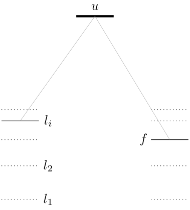
Figure 1: Schematic diagram of the $\Lambda$-type multi-term atom. In order to correctly describe the polarization properties of the outgoing light in the $u\to f$ transition, all lower terms $l_{i}$ that are radiatively or collisionally connected to the upper term $u$, including the final term $f$, must be taken into account.

Among the various theoretical approaches to the problem of polarized radiative transfer (RT) with PRD, the two advanced by Bommier (1997a, b, 2016) and by Casini and collaborators (Casini et al., 2014; Casini & Manso Sainz, 2016) have in particular come under some in-depth scrutiny. Both approaches rely on a derivation of the respective formalisms from the first principles of non-relativistic quantum electrodynamics, yet they have led to seemingly different interpretations of the driving physical processes of radiation scattering (see the discussions in Casini et al., 2014; Bommier, 2016, 2017).

The problem of determining the proper expressions of the branching ratios for the fully redistributed (CRD) and the partially redistributed contributions of the polarized emissivity to the RT equation in a collisional plasma has recently been considered within both approaches. This is one of the key problems for the validation of any theoretical description of radiation scattering, and ultimately for its applicability to the numerical modeling of polarized RT in a magnetized chromosphere. Casini, del Pino Alemán, & Manso Sainz (2017) have derived a very general form of the scattering emissivity, which is broadly applicable to numerical problems of polarized radiation scattering in multi-term atoms of the $\Lambda$-type (Casini & Manso Sainz, 2016, see also Figure 1). Bommier (2017) has explicitly derived the expressions of the branching ratios for the CRD and PRD contributions to the emissivity redistribution function for the case of a two-term atom with non-coherent and unpolarized lower term.

In this work we show how the two approaches lead to branching ratios that are in full agreement, when the generalized form of the emissivity of Casini, del Pino Alemán, & Manso Sainz (2017) is explicitly applied to the same atomic model considered by Bommier (2017).

2 General form of the polarized scattering emissivity

We consider the general expression of the polarized radiation emissivity proposed by Casini, del Pino Alemán, & Manso Sainz (2017), describing the partially coherent scattering of radiation in spectral lines from permitted transitions that are formed under PRD conditions. This emissivity represents the source term of the vector transfer equation for polarized radiation,

$$\frac{d}{ds}\,\bm{S}(\omega_{k^{\prime}},\bm{\hat{k}}^{\prime})=-{\bf K}(\omega_{k^{\prime}},\bm{\hat{k}}^{\prime})\,\bm{S}(\omega_{k^{\prime}},\bm{\hat{k}}^{\prime})+\bm{\varepsilon}(\omega_{k^{\prime}},\bm{\hat{k}}^{\prime})\;,$$ (1)

where $\bm{S}\equiv(S_{0},S_{1},S_{2},S_{3})$ is the Stokes vector of the polarized radiation field (of frequency $\omega_{k^{\prime}}$ and propagation direction $\bm{\hat{k}}^{\prime}$), $\bf K$ is the 4$\times$4 polarized absorption matrix (responsible for both isotropic and dichroic absorption, as well as magneto-optical effects), and

$$\bm{\varepsilon}(\omega_{k^{\prime}},\bm{\hat{k}}^{\prime})\equiv\Bigl{[}\bm{\varepsilon}^{\mbox{\tiny{(1)}}}(\omega_{k^{\prime}},\bm{\hat{k}}^{\prime})-\bm{\varepsilon}^{\mbox{\tiny{(2)}}}(\omega_{k^{\prime}},\bm{\hat{k}}^{\prime})_{\rm f.s.}\Bigr{]}+\bm{\varepsilon}^{\mbox{\tiny{(2)}}}(\omega_{k^{\prime}},\bm{\hat{k}}^{\prime})\;,$$ (2)

is the generalized emissivity. For a multi-term atomic system of the $\Lambda$-type (see Figure 1), the first-order emissivity in the atomic frame of reference is given by

$$\varepsilon^{\mbox{\tiny{(1)}}}_{i}(\omega_{k^{\prime}},\bm{\hat{k}}^{\prime}) = \frac{1}{2\pi^{2}\sqrt{3}}\,\frac{e_{0}^{2}}{c^{3}}\,{\cal N}\omega_{k^{\prime}}^{4}\sum_{uu^{\prime}}\rho_{uu^{\prime}}\sum_{f}\sum_{pp^{\prime}}(-1)^{p^{\prime}+1}\,(r_{p})_{u^{\prime}f}(r_{p^{\prime}})_{uf}^{*}$$

$${}\times\sum_{K^{\prime}Q^{\prime}}\sqrt{2K^{\prime}+1}\,\biggl{(}\begin{matrix}1&1&K^{\prime}\\ -p&p^{\prime}&-Q^{\prime}\\ \end{matrix}\biggr{)}\,T^{K^{\prime}}_{Q^{\prime}}(i,\bm{\hat{k}}^{\prime})\Bigl{(}\Phi_{fu^{\prime}}^{+k^{\prime}}+\bar{\Phi}_{fu}^{+k^{\prime}}\Bigr{)}\;,\qquad(i=0,1,2,3)$$

where we introduced the usual complex line profiles,

$$\Phi_{ab}^{\pm k}\equiv\frac{\rm i}{\omega_{ba}\mp\omega_{k}+{\rm i}\epsilon_{ba}}\;,$$

and we indicated with $\bar{\Phi}$ the operation of complex conjugation. For the definition of all the other physical quantities in equation (2) and in the following equations, we refer to Casini et al. (2014). Making use of the conjugation properties of those various quantities, it is possible to show that this emissivity term is purely real. In particular, this is a direct consequence of the hermiticity of the density-matrix $\rho_{uu^{\prime}}$ for the upper term.

The contribution (2) to the general emissivity is associated with excitation mechanisms of the upper term that lead to the production of completely redistributed radiation, i.e., to fully non-coherent scattering of the incident radiation. As an example, this term accounts for the emission of radiation via the spontaneous decay of a collisionally excited level.

For typical applications to astrophysical plasmas, it is safe to assume that the incident radiation field is highly diluted (weak radiation field approximation), so that the radiative lifetime of the lower atomic levels is practically infinite compared to their collisional lifetime. Under this assumption, radiation absorption does not contribute appreciably to the population of the upper state (Casini et al., 2014). Therefore, that population is for practical purposes completely determined by the balance between collisional excitation and spontaneous de-excitation (because of the weak radiation field assumption, all stimulated radiation processes can also be neglected).

The second-order emissivity, which accounts for two-photon processes in a $\Lambda$-type atom leading to partially redistributed scattering, in the atomic frame of reference is given by (see Casini et al., 2014)

$$\varepsilon^{\mbox{\tiny{(2)}}}_{i}(\omega_{k^{\prime}},\bm{\hat{k}}^{\prime}) = \frac{4}{3}\frac{e_{0}^{4}}{\hbar^{2}c^{4}}\,{\cal N}\omega_{k^{\prime}}^{4}\sum_{ll^{\prime}}\rho_{ll^{\prime}}\sum_{uu^{\prime}f}\sum_{qq^{\prime}}\sum_{pp^{\prime}}(-1)^{q^{\prime}+p^{\prime}}\,(r_{q})_{ul}(r_{q^{\prime}})^{\ast}_{u^{\prime}l^{\prime}}(r_{p})_{u^{\prime}f}(r_{p^{\prime}})^{\ast}_{uf}$$ (4)

$$\times\sum_{KQ}\sum_{K^{\prime}Q^{\prime}}\sqrt{(2K+1)(2K^{\prime}+1)}\,\biggl{(}\begin{matrix}1&1&K\\ -q&q^{\prime}&-Q\\ \end{matrix}\biggr{)}\biggl{(}\begin{matrix}1&1&K^{\prime}\\ -p&p^{\prime}&-Q^{\prime}\\ \end{matrix}\biggr{)}\,T^{K^{\prime}}_{Q^{\prime}}(i,\bm{\hat{k}}^{\prime})$$

$$\times\int_{0}^{\infty}d\omega_{k}\,\Bigl{(}\Psi_{u^{\prime}l^{\prime},ful}^{-k,+k^{\prime}-k}+\bar{\Psi}_{ul,fu^{\prime}l^{\prime}}^{-k,+k^{\prime}-k}\Bigr{)}\,J^{K}_{Q}(\omega_{k})\;,\qquad(i=0,1,2,3)$$

where

$$\Psi_{ab,cde}^{\pm h,\pm k\pm l} \equiv \frac{-{\rm i}}{(\omega_{ac}\pm\omega_{h}\mp\omega_{l}\mp\omega_{k}+{\rm i}\epsilon_{a}+{\rm i}\epsilon_{c})(\omega_{ad}\pm\omega_{h}\mp\omega_{l}+{\rm i}\epsilon_{a}+{\rm i}\epsilon_{d})(\omega_{ae}\pm\omega_{h}+{\rm i}\epsilon_{a}+{\rm i}\epsilon_{e})}$$ (5)

$$+ \frac{-{\rm i}}{(\omega_{ac}\pm\omega_{h}\mp\omega_{l}\mp\omega_{k}+{\rm i}\epsilon_{a}+{\rm i}\epsilon_{c})(\omega_{bc}\mp\omega_{l}\mp\omega_{k}+{\rm i}\epsilon_{b}+{\rm i}\epsilon_{c})(\omega_{cd}\pm\omega_{k}-{\rm i}\epsilon_{c}+{\rm i}\epsilon_{d})}$$

$$- \frac{-{\rm i}}{(\omega_{ad}\pm\omega_{h}\mp\omega_{l}+{\rm i}\epsilon_{a}+{\rm i}\epsilon_{d})(\omega_{bd}\mp\omega_{l}+{\rm i}\epsilon_{b}+{\rm i}\epsilon_{d})(\omega_{cd}\pm\omega_{k}-{\rm i}\epsilon_{c}+{\rm i}\epsilon_{d})}\;,$$

and with $\bar{\Psi}$ we indicated the complex conjugate of the profile $\Psi$. The frequency integral in equation (4) can be rewritten in terms of the redistribution function ${\cal R}(\omega_{k},\omega_{k^{\prime}})$ for a three-term $\Lambda$-atom, using the definition (4) of Casini, del Pino Alemán, & Manso Sainz (2017; see also Casini et al. 2014, equation (6)),

$${\cal R}(\Omega_{u},\Omega_{u^{\prime}};\Omega_{l},\Omega_{l^{\prime}},\Omega_{f};\omega_{k},\omega_{k^{\prime}})={\rm i}(\Omega_{u}-\Omega_{u^{\prime}}^{\ast})\Bigl{(}\Psi_{u^{\prime}l^{\prime},ful}^{-k,+k^{\prime}-k}+\bar{\Psi}_{ul,fu^{\prime}l^{\prime}}^{-k,+k^{\prime}-k}\Bigr{)}\;,$$ (6)

where we introduced the complex atomic frequencies $\Omega_{a}=\omega_{a}-{\rm i}\epsilon_{a}$.

The subscript “f.s.” in one of the two second-order terms of the general emissivity in equation (2) means that such term must be evaluated as if the incident radiation field were spectrally flat, i.e., described by some average $J^{K}_{Q}(\bar{\omega}$) of the incident radiation field tensor across the atomic transition. For the moment, we leave aside the question of what such a suitable average should look like, and simply observe that an immediate result of that averaging procedure is the ability to perform the integration over the incident frequency $\omega_{k}$ in equation (4). This is simply attained by recalling the following integral norm of the redistribution function (cf. Casini et al., 2014, equation (15)),

$$\int_{0}^{\infty}d\omega_{k}\,\Bigl{(}\Psi_{u^{\prime}l^{\prime},ful}^{-k,+k^{\prime}-k}+\bar{\Psi}_{ul,fu^{\prime}l^{\prime}}^{-k,+k^{\prime}-k}\Bigr{)}=\frac{2\pi}{\epsilon_{uu^{\prime}}+{\rm i}\omega_{uu^{\prime}}}\,\Bigl{(}\Phi_{fu^{\prime}}^{+k^{\prime}}+\bar{\Phi}_{fu}^{+k^{\prime}}\Bigr{)}\;.$$ (7)

Substitution of this integral expression into equation (4) immediately yields

$$\varepsilon^{\mbox{\tiny{(2)}}}_{i}(\omega_{k^{\prime}},\bm{\hat{k}}^{\prime})_{\rm f.s.} = \frac{4}{3}\frac{e_{0}^{4}}{\hbar^{2}c^{4}}\,{\cal N}\omega_{k^{\prime}}^{4}\sum_{ll^{\prime}}\rho_{ll^{\prime}}\sum_{uu^{\prime}f}\sum_{qq^{\prime}}\sum_{pp^{\prime}}(-1)^{q^{\prime}+p^{\prime}}\,(r_{q})_{ul}(r_{q^{\prime}})^{\ast}_{u^{\prime}l^{\prime}}(r_{p})_{u^{\prime}f}(r_{p^{\prime}})^{\ast}_{uf}$$ (8)

$${}\times\sum_{KQ}\sum_{K^{\prime}Q^{\prime}}\sqrt{(2K+1)(2K^{\prime}+1)}\,\biggl{(}\begin{matrix}1&1&K\\ -q&q^{\prime}&-Q\\ \end{matrix}\biggr{)}\biggl{(}\begin{matrix}1&1&K^{\prime}\\ -p&p^{\prime}&-Q^{\prime}\\ \end{matrix}\biggr{)}\,T^{K^{\prime}}_{Q^{\prime}}(i,\bm{\hat{k}}^{\prime})$$

$$\kern 56.9055pt{}\times\frac{2\pi}{\epsilon_{uu^{\prime}}+{\rm i}\omega_{uu^{\prime}}}\,\Bigl{(}\Phi_{fu^{\prime}}^{+k^{\prime}}+\bar{\Phi}_{fu}^{+k^{\prime}}\Bigr{)}\,J^{K}_{Q}(\bar{\omega})$$

$$= \frac{1}{2\pi^{2}\sqrt{3}}\,\frac{e_{0}^{2}}{c^{3}}\,{\cal N}\omega_{k^{\prime}}^{4}\sum_{uu^{\prime}}\Biggl{[}\frac{16\pi^{3}}{\sqrt{3}}\frac{e_{0}^{2}}{\hbar^{2}c}\,\frac{1}{\epsilon_{uu^{\prime}}+{\rm i}\omega_{uu^{\prime}}}\sum_{ll^{\prime}}\rho_{ll^{\prime}}\sum_{qq^{\prime}}(-1)^{q^{\prime}+1}\,(r_{q})_{ul}(r_{q^{\prime}})^{\ast}_{u^{\prime}l^{\prime}}$$

$$\kern 99.58464pt{}\times\sum_{KQ}\sqrt{2K+1}\,\biggl{(}\begin{matrix}1&1&K\\ -q&q^{\prime}&-Q\\ \end{matrix}\biggr{)}J^{K}_{Q}(\bar{\omega})\Biggr{]}$$

$${}\times\sum_{f}\sum_{pp^{\prime}}(-1)^{p^{\prime}+1}\,(r_{p})_{u^{\prime}f}(r_{p^{\prime}})^{\ast}_{uf}\sum_{K^{\prime}Q^{\prime}}\sqrt{2K^{\prime}+1}\,\biggl{(}\begin{matrix}1&1&K^{\prime}\\ -p&p^{\prime}&-Q^{\prime}\\ \end{matrix}\biggr{)}$$

$$\kern 99.58464pt{}\times T^{K^{\prime}}_{Q^{\prime}}(i,\bm{\hat{k}}^{\prime})\Bigl{(}\Phi_{fu^{\prime}}^{+k^{\prime}}+\bar{\Phi}_{fu}^{+k^{\prime}}\Bigr{)}\;.\qquad(i=0,1,2,3)$$

A direct comparison of this result with equation (2) shows that the two expressions of $\varepsilon^{\mbox{\tiny{(1)}}}$ and $\varepsilon^{\mbox{\tiny{(2)}}}_{\rm f.s.}$ coincide when the quantity inside the square brackets in equation (8) can be identified with the upper-term atomic density matrix $\rho_{uu^{\prime}}$ (Casini et al., 2014, Section 7). This is indeed the case for the solution of the first-order statistical equilibrium (SE) problem for the multi-term atom of the $\Lambda$-type in the presence of only radiative processes, involving one-photon absorption and emission, when stimulated emission is negligible (weak radiation field approximation). In this limit, the identification of $\rho_{uu^{\prime}}$ with the expression inside the square brackets in equation (8) implies that $J^{K}_{Q}(\bar{\omega})$ must correspond to the integral average of the incident radiation field tensor that appears in the transfer rate for radiative absorption of the first-order SE problem (cf. Landi Degl’Innocenti, 1983, 1984). This rate is given by

$$t_{\rm A}(uu^{\prime},ll^{\prime}) = \frac{16\pi^{3}}{\sqrt{3}}\frac{e_{0}^{2}}{\hbar^{2}c}\,\sum_{qq^{\prime}}(-1)^{q+q^{\prime}}(r_{q})_{ul}(r_{q^{\prime}})_{u^{\prime}l^{\prime}}^{\ast}\sum_{KQ}\sqrt{2K+1}\,\biggl{(}\begin{matrix}1&1&K\\ -q&q^{\prime}&-Q\\ \end{matrix}\biggr{)}$$ (9)

$${}\times\frac{1}{2\pi}\int_{0}^{\infty}d\omega_{k}\,\Bigl{(}\Phi_{l^{\prime}u^{\prime}}^{+k}+\bar{\Phi}_{lu}^{+k}\Bigr{)}\,J^{K}_{Q}(\omega_{k})\;,$$

hence,

$$J^{K}_{Q}(\bar{\omega})=J^{K}_{Q}(\omega_{ul;u^{\prime}l^{\prime}})\equiv\frac{1}{2\pi}\int_{0}^{\infty}d\omega_{k}\,\Bigl{(}\Phi_{l^{\prime}u^{\prime}}^{+k}+\bar{\Phi}_{lu}^{+k}\Bigr{)}\,J^{K}_{Q}(\omega_{k})\;.$$ (10)

For the following development, we adopt equation (10) as the proper definition of the integral average $J^{K}_{Q}(\bar{\omega})$ entering equation (8).

It must be noted that such “average” generally takes different values for different pairs of atomic transition components $(ul;u^{\prime}l^{\prime})$. In this sense, the adoption of equation (10) actually implies a full departure of the SE solution from the limitations of the flat-spectrum approximation, which instead requires that the incident radiation field tensor $J^{K}_{Q}(\omega_{k})$ must be structureless over the entire spectral range spanned by all the components of the atomic transition. This is a critical aspect of our formalism, since the flat-spectrum approximation is instead a necessary condition for the physical consistency of the first-order RT problem, where the emissivity term is represented exclusively by $\bm{\varepsilon}^{\mbox{\tiny{(1)}}}$. In our case, instead, use of the expression (2) for the total emissivity allows us to relax the condition of the flat-spectrum approximation in the first-order SE problem without breaking the internal consistency of the description of the scattering process.

In contrast, the appearance of the average radiation tensor $J^{K}_{Q}(\bar{\omega})$ in the $\bm{\varepsilon}^{\mbox{\tiny{(2)}}}_{\rm f.s.}$ emissivity does require replacing the incident radiation field in $\bm{\varepsilon}^{\mbox{\tiny{(2)}}}$ by an appropriate constant average for each of the transition components, according to the definition (10). Hence the reason to dub that emissivity term as a “flat spectrum” contribution to the total emissivity.

In many practical cases of interest to solar polarimetry, the incident radiation field will largely be constant over the typical frequency separation of the Zeeman components of the line in the presence of a magnetic field, whereas it might have a significant spectral modulation over the frequency range of the atomic fine structure, depending on the nature of the multiplets. This is certainly the case, e.g., for well-known doublets of the solar spectrum, such as Mg II h–k, Ca II H–K, or Na I D₁–D₂, whereas for close spectral multiplets, such as H I Ly_α and H_α, the spectral modulation of the incident radiation field across the fine structure is generally unimportant. Therefore, in many applications it might be possible to consider only a reduced set of integral averages of the type $J^{K}_{Q}(\omega_{J_{u}J_{l};J_{u}^{\prime}J_{l}^{\prime}})$, thus simplifying the numerical implementation of the line formation problem.

It is important to note that the exact cancellation between $\bm{\varepsilon}^{\mbox{\tiny{(1)}}}$ and $\bm{\varepsilon}^{\mbox{\tiny{(2)}}}_{\rm f.s.}$ in the purely radiative case embodies our original assumption of infinite radiative lifetime of the lower terms, according to which no population of the upper term can actually be created through radiative absorption. In this second-order framework, the two independent, first-order processes of absorption and re-emission of a single photon are instead replaced by a single, coherent two-photon process represented by $\bm{\varepsilon}^{\mbox{\tiny{(2)}}}$.

In order to combine the contributions (2), (4), and (8) into the general emissivity (2), in the presence of both radiative and collisional processes, we must formally solve the SE problem of the atomic system for the density matrix $\rho_{uu^{\prime}}$ of the upper state under such more general case.

For an isotropic distribution of colliding perturbers, assuming the validity of the impact approximation for collisions, it can be shown (see, e.g., Belluzzi, Landi Degl’Innocenti, & Trujillo Bueno, 2013) that the algebraic solution for $\rho_{uu^{\prime}}$ can be generalized beyond the purely radiative expression inside the square brackets of equation (8). Simply put, the radiative width $\epsilon_{uu^{\prime}}$ for the upper term is augmented by the inverse lifetime for collisional relaxation of the excited levels, whereas a collisional excitation term is added to the SE problem alongside the radiative excitation term corresponding to the $t_{\rm A}$ transfer rate (9). The dominant effect of this last contribution from collisional excitation is the tendency of the system towards thermalization of the atomic populations, with a corresponding contribution to the first-order emissivity that essentially corresponds to a Planckian radiation at the equilibrium temperature of the plasma. Accordingly, the solution density matrix for the upper term appearing in equation (2) can be written as the sum of a radiative and a collisional part (Casini, del Pino Alemán, & Manso Sainz, 2017),

$$\rho_{uu^{\prime}}=\rho_{uu^{\prime}}^{\mbox{\tiny{(rad)}}}+\rho_{uu^{\prime}}^{\mbox{\tiny{(coll)}}}\;,$$

and correspondingly we can write, from equation (2),

$$\bm{\varepsilon}^{\mbox{\tiny{(1)}}}(\omega_{k^{\prime}},\bm{\hat{k}}^{\prime})=\bm{\varepsilon}^{\mbox{\tiny{(1;rad)}}}(\omega_{k^{\prime}},\bm{\hat{k}}^{\prime})+\bm{\varepsilon}^{\mbox{\tiny{(1;coll)}}}(\omega_{k^{\prime}},\bm{\hat{k}}^{\prime})\;.$$ (11)

In the absence of elastic collisions, the (nearly Planckian) term in equation (11) associated with $\rho_{uu^{\prime}}^{\mbox{\tiny{(coll)}}}$ is the only completely redistributed contribution to the scattered radiation, since the contribution from $\rho_{uu^{\prime}}^{\mbox{\tiny{(rad)}}}$ is exactly compensated by $\bm{\varepsilon}^{\mbox{\tiny{(2)}}}_{\rm f.s.}$ (cf. equation (8), and the discussion after equation (10)). When instead elastic collisions are present, the denominator ${\rm i}(\Omega_{u}-\Omega_{u^{\prime}}^{\ast})$ that appears in the expression of $\bm{\varepsilon}^{\mbox{\tiny{(2)}}}$ (cf. equation (6)) must also account for the additional level width $\Gamma_{uu^{\prime}}$ due to the perturbation of the atomic levels by the elastic colliders. In contrast, because elastic collisions do not affect the population balance in the first-order SE problem, a corresponding contribution is instead missing from the denominator $\epsilon_{uu^{\prime}}+{\rm i}\omega_{uu^{\prime}}$ appearing in the formal expression of $\rho_{uu^{\prime}}^{\mbox{\tiny{(rad)}}}$. Hence, an exact compensation between $\bm{\varepsilon}^{\mbox{\tiny{(1;rad)}}}$ and $\bm{\varepsilon}^{\mbox{\tiny{(2)}}}_{\rm f.s.}$ generally no longer occurs in the presence of elastic collisions.

In conclusion, we can rewrite the general emissivity (2) as

$$\bm{\varepsilon}(\omega_{k^{\prime}},\bm{\hat{k}}^{\prime}) = \bm{\varepsilon}^{\mbox{\tiny{(1;coll)}}}(\omega_{k^{\prime}},\bm{\hat{k}}^{\prime})+\bm{\tilde{\varepsilon}}(\omega_{k^{\prime}},\bm{\hat{k}}^{\prime})$$ (12)

$$= \bm{\varepsilon}^{\mbox{\tiny{(1;coll)}}}(\omega_{k^{\prime}},\bm{\hat{k}}^{\prime})+\left[\bm{\varepsilon}^{\mbox{\tiny{(1;rad)}}}(\omega_{k^{\prime}},\bm{\hat{k}}^{\prime})-\bm{\varepsilon}^{\mbox{\tiny{(2)}}}_{\rm f.s.}(\omega_{k^{\prime}},\bm{\hat{k}}^{\prime})\right]+\bm{\varepsilon}^{\mbox{\tiny{(2)}}}(\omega_{k^{\prime}},\bm{\hat{k}}^{\prime})\;,$$

and recalling equations (2), (4), and (8), after some straightforward algebra, we find

$$\tilde{\varepsilon}_{i}(\omega_{k^{\prime}},\bm{\hat{k}}^{\prime}) = \frac{4}{3}\frac{e_{0}^{4}}{\hbar^{2}c^{4}}\,{\cal N}\omega_{k^{\prime}}^{4}\sum_{ll^{\prime}}\rho_{ll^{\prime}}\sum_{uu^{\prime}f}\sum_{qq^{\prime}}\sum_{pp^{\prime}}(-1)^{q^{\prime}+p^{\prime}}\,(r_{q})_{ul}(r_{q^{\prime}})^{\ast}_{u^{\prime}l^{\prime}}(r_{p})_{u^{\prime}f}(r_{p^{\prime}})^{\ast}_{uf}$$ (13)

$$\times\sum_{KQ}\sum_{K^{\prime}Q^{\prime}}\sqrt{(2K+1)(2K^{\prime}+1)}\,\biggl{(}\begin{matrix}1&1&K\\ -q&q^{\prime}&-Q\\ \end{matrix}\biggr{)}\biggl{(}\begin{matrix}1&1&K^{\prime}\\ -p&p^{\prime}&-Q^{\prime}\\ \end{matrix}\biggr{)}\,T^{K^{\prime}}_{Q^{\prime}}(i,\bm{\hat{k}}^{\prime})$$

$$\times\int_{0}^{\infty}d\omega_{k}\;\mathscr{R}(\Omega_{u},\Omega_{u^{\prime}};\Omega_{l},\Omega_{l^{\prime}},\Omega_{f};\omega_{k},\omega_{k^{\prime}})\,J^{K}_{Q}(\omega_{k})\;,\qquad(i=0,1,2,3)$$

where we introduced the generalized redistribution function in the atomic frame of reference,

$${\mathscr{R}}(\Omega_{u},\Omega_{u^{\prime}};\Omega_{l},\Omega_{l^{\prime}},\Omega_{f};\omega_{k},\omega_{k^{\prime}}) = \frac{1}{\epsilon_{uu^{\prime}}+\Gamma_{uu^{\prime}}+{\rm i}\omega_{uu^{\prime}}}\,{\cal R}(\Omega_{u},\Omega_{u^{\prime}};\Omega_{l},\Omega_{l^{\prime}},\Omega_{f};\omega_{k},\omega_{k^{\prime}})$$

$$\kern-56.9055pt+\left(\frac{1}{\epsilon_{uu^{\prime}}+{\rm i}\omega_{uu^{\prime}}}-\frac{1}{\epsilon_{uu^{\prime}}+\Gamma_{uu^{\prime}}+{\rm i}\omega_{uu^{\prime}}}\right)\!\Bigl{(}\Phi_{l^{\prime}u^{\prime}}^{+k}+\bar{\Phi}_{lu}^{+k}\Bigr{)}\Bigl{(}\Phi_{fu^{\prime}}^{+k^{\prime}}+\bar{\Phi}_{fu}^{+k^{\prime}}\Bigr{)}\;,$$

and where ${\cal R}(\omega_{k},\omega_{k^{\prime}})$ is given by equation (6), while we considered that ${\rm i}(\Omega_{u}-\Omega_{u^{\prime}}^{\ast})=\epsilon_{uu^{\prime}}+\Gamma_{uu^{\prime}}+{\rm i}\omega_{uu^{\prime}}$, in the additional presence of elastic collisions. According to the previous discussion, the average radiation tensor (10) must be adopted for both equations (2) and (8) in order to arrive at equation (2).

The non-Planckian emissivity (13) can further be specialized to particular atomic structures, such as the multi-term atom of the $\Lambda$-type in the $LS$-coupling scheme, with and without hyperfine structure, and the multi-level atom. This is immediately accomplished by taking equations (4), (7), and (8) of Casini & Manso Sainz (2016), respectively, for those three atomic models, and substituting the redistribution integral of equation (13) in those equations, using the definition (2), while at the same time omitting from those earlier equations the factor $1/(\epsilon_{uu^{\prime}}+{\rm i}\omega_{uu^{\prime}})$, as this is already accounted for, in a more general form, by the redistribution function (2).

With this straightforward exercise, we can verify that our second-order emissivity (13) and generalized redistribution function (2) agree with those derived by Bommier (2017) for the case of the two-term atom with non-coherent lower term (i.e., $\rho_{ll^{\prime}}=\delta_{ll^{\prime}}\rho_{ll}$) and infinitely sharp lower levels (i.e., $\epsilon_{l},\epsilon_{f}\to 0$), once the redistribution function ${\cal R}(\omega_{k},\omega_{k^{\prime}})$ is replaced by the appropriate expression for this case (Casini et al., 2014, equation (10)). In particular, depolarizing collisions can also be included analogously to Bommier (2017), taking into consideration the corresponding contributions to the first-order SE problem. In such case, a new level width contribution is added to the denominator of $1/(\epsilon_{uu^{\prime}}+{\rm i}\omega_{uu^{\prime}})$ in the second line of equation (2), as a consequence of this modification for the atomic density matrix solution of the SE problem (see Bommier, 2017).

3 Conclusions

We derived the explicit form of the branching ratios for the contributions of completely redistributed radiation and of partially coherent scattering to the generalized emissivity in the radiative transfer equation for polarized radiation. The expression for this emissivity was proposed by Casini, del Pino Alemán, & Manso Sainz (2017) in the implicit form of equation (2). In this work, we considered the algebraic expressions of its various contributions, and demonstrated how they combine to give rise to a new form of the second-order emissivity for partially coherent scattering in a two-term atom proposed by Casini et al. (2014) (see also Casini & Manso Sainz 2016 for its extension to the three-term atom of the $\Lambda$-type). In this emissivity, the usual partial redistribution function is replaced by a more general expression, equation (2), which also takes into account the contribution of fully redistributed radiation caused by collisional processes.

In the limit of the two-term atom with non-coherent lower term, the generalized redistribution function (2) proves to be identical to the one recently derived by Bommier (2017) through her own ab-initio formulation of the polarized scattering problem. This verification confirms that the two independent formalisms of Bommier (1997a, b, 2016, 2017) and of Casini et al. (2014), Casini & Manso Sainz (2016), and Casini, del Pino Alemán, & Manso Sainz (2017), though seemingly different, are in fact complementary, and lead to exactly the same predictions for the properties of the partially redistributed polarized radiation scattered by a two-term atom. In particular, the adoption of equation (2) for the total emissivity of the radiative transfer problem—and of equation (2) for the CRD and PRD branching ratios—allows us to completely relax the limitation of the flat-spectrum approximation in the solution of the first-order statistical equilibrium problem (see also Bommier, 2017). Accordingly, the statistical equilibrium problem underlying the formation of spectral lines under PRD conditions corresponds to the original formulation of Landi Degl’Innocenti (1983, 1984), as originally pointed out by Bommier (1997a, b).

As a final remark, it is important to point out that while the derivation of the generalized redistribution function in the explicit form (2) relied specifically on the choice of a reference frame at rest with the atom, the implicit form given by equation (2) is instead generally valid, and thus it is immediately applicable to numerical problems of polarized radiative transfer in model atmospheres. Such approach was followed by del Pino Alemán, Casini, & Manso Sainz (2016) for the modeling of the Mg II h–k doublet in a magnetized chromosphere including PRD effects.

References

• Alsina Ballester, Belluzzi, & Trujillo Bueno (2016) Alsina Ballester, E., Belluzzi, L., & Trujillo Bueno, J. 2016, ApJ, 831, 15
• Belluzzi, Landi Degl’Innocenti, & Trujillo Bueno (2013) Belluzzi, L., Landi Degl’Innocenti, E., & Trujillo Bueno, J. 2013, A&A, 551, 84
• Bommier (1997a) Bommier, V. 1997a, A&A, 328, 706
• Bommier (1997b) Bommier, V. 1997b, A&A, 328, 726
• Bommier (2016) Bommier, V. 2016, A&A, 591A, 59
• Bommier (2017) Bommier, V. 2017, A&A (in press)
• Bommier & Stenflo (1999) Bommier, V., & Stenflo, J. O. 1999, A&A, 350, 327
• Casini et al. (2014) Casini, R., Landi Degl’Innocenti, M., Manso Sainz, R., Landi Degl’Innocenti, M., & Landolfi, M. 2014, ApJ, 791, 94
• Casini & Manso Sainz (2016) Casini, R., & Manso Sainz, R. 2016, ApJ, 824, 135
• Casini, del Pino Alemán, & Manso Sainz (2017) Casini, R., del Pino Alemán, T., & Manso Sainz, R. 2017, ApJ, 835, 114
• del Pino Alemán, Casini, & Manso Sainz (2016) del Pino Alemán, T., Casini, R., & Manso Sainz, R. 2016, ApJ, 830, L24
• Landi Degl’Innocenti (1983) Landi Degl’Innocenti, E. 1983, Sol. Phys., 85, 3
• Landi Degl’Innocenti (1984) Landi Degl’Innocenti, E. 1984, Sol. Phys., 91, 1
• Landi Degl’Innocenti & Landolfi (2004) Landi Degl’Innocenti, E., & Landolfi, M. 2004, Polarization in Spectral Lines (Dordrecht: Springer)
• Landi Degl’Innocenti, Landi Degl’Innocenti, & Landolfi (1997) Landi Degl’Innocenti, E., Landi Degl’Innocenti, M., & Landolfi, M. 1997, in Proc. Forum THÉMIS, Science with THÉMIS, ed. N. Mein & S. Sahal-Bréchot (Paris: Obs. Paris-Meudon), 59
• Sowmya et al. (2014) Sowmya, K., Nagendra, K. N., Sampoorna, M., & Stenflo, J. O. 2014, ApJ, 793, 71
• Trujillo Bueno, Štěpán, & Casini (2011) Trujillo Bueno, J., Štěpán, J., & Casini, R. 2011, ApJ, 738, 11