Measurement of Reconstructed Charged Particle Multiplicities of Neutrino Interactions in MicroBooNE
Talk presented at the APS Division of Particles and Fields Meeting (DPF 2017), July 31-August 4, 2017, Fermilab. C170731

Abstract

We compare the observed charged particle multiplicity distributions in the MicroBooNE liquid argon time projection chamber from neutrino interactions in a restricted final state phase space to predictions of this distribution from several GENIE models. The measurement uses a data sample consisting of neutrino interactions with a final state muon candidate fully contained within the MicroBooNE detector.  These data were collected in 2015-2016 with the Fermilab Booster Neutrino Beam (BNB), which has an average neutrino energy of $800$ MeV, using an exposure corresponding to $5.0\times 10^{19}$ protons-on-target.  The analysis employs fully automatic event selection and charged particle track reconstruction and uses a data-driven technique to determine the contribution to each multiplicity bin from neutrino interactions and cosmic-induced backgrounds. The restricted phase space employed makes the measurement most sensitive to the higher-energy charged particles expected from primary neutrino-argon collisions and less sensitive to lower energy protons expected to be produced in final state interactions of collision products with the target argon nucleus.

1 Introduction

1.1 Observed Charged Particle Multiplicity Distribution

Neutrino interactions in the MicroBooNE detector [1] produce charged particles that can be reconstructed as tracks in the liquid argon medium of the active time projection chamber (TPC) volume of the detector. The charged particle multiplicity, or number of primary charged stable particles $n$, is a simple observable characterizing final states in high-energy-collision processes, including neutrino interactions. We note that in MicroBooNE the observable charged particle multiplicity corresponds to that of charged particles exiting the target nucleus participating in the neutrino interaction. The charged particle multiplicity distribution (CPMD) comprise the set of probabilities, $P_{n}$, associated with producing $n$ charged particles in a neutrino event, either in full phase space or in restricted phase space domains.

Determination of the CPMD at Fermilab Booster Neutrino Beam (BNB) [2] neutrino energies naturally fits into the modern strategy [3] of presenting neutrino interaction measurements in the form of directly observable quantities.  The CPMD measurements expand the empirical knowledge of neutrino-argon scattering that will be required by the DUNE experiment [4]. As physical observable, the CPMD can also be used to test neutrino cross-section models, or particular tunes of generators such as GENIE [5].  These models are typically constructed from a set of exclusive cross section channels, and the inclusive character of CPMD thus provides independent checks.

This note describes a preliminary test of several variants of GENIE against the observed charged particle multiplicity distribution (observed CPMD) in MicroBooNE data collected during the 2015-2016 time period at the Fermilab BNB.  By “observed”, we mean the probability, after application of certain detector selection requirements, of observing a neutrino interaction with $n$ charged tracks. We present this relative to the probability of observing a neutrino interaction with at least one charged track:

$$O_{n}=\frac{N_{\text{obs,}n}}{\sum\limits_{m=1}^{M_{\text{obs},\max}}N_{\text{obs,}m}},$$ (1)

where $N_{\text{obs,}n}$ is the number of neutrino interaction events with $n$ observed tracks, and $M_{\text{obs},\max}$ is the maximum observed value for $N_{\text{obs,}n}$.  At BNB energies, $M_{\text{obs},\max}\approx 5$. Our analysis requires at least one of the charged tracks to be consistent with a muon; hence the $O_{n}$ are effectively observed CPMD for $\nu_{\mu}$ charged current ($\nu_{\mu}$ CC) interactions.  The muon candidate is included in the charged particle multiplicity, and all events thus have $n\geq 1$.

The values for $O_{n}$ depend on cross sections for producing a multiplicity $n$, $\sigma_{CC,n}$ as well as the BNB neutrino flux and detector acceptance and efficiency:

$$N_{\text{obs,}n}=\sum_{n^{\prime}}\int dE_{\nu}\Phi_{\nu}\left(E_{\nu}\right)\int d\Pi_{n^{\prime}}\frac{d\sigma_{CC,n^{\prime}}\left(E_{\nu},\Omega\right)}{d\Pi_{n^{\prime}}}\epsilon_{n,n^{\prime}}\left(E_{\nu},\Pi_{n^{\prime}}\right),$$ (2)

where $E_{\nu}$ is the neutrino energy, $\Phi_{\nu}\left(E_{\nu}\right)$ is the neutrino flux, $d\Pi_{n}$ represents the $n$-particle final state phase space, $\epsilon_{n,n^{\prime}}\left(E_{\nu},\Omega\right)$ is an acceptance and efficiency matrix that gives the probability that an $n^{\prime}$ charged particle final state produced in phase space element $d\Pi_{n^{\prime}}$ is observed as an $n$-particle final state in the detector, and $d\sigma_{CC,n^{\prime}}\left(E_{\nu},\Omega\right)/d\Pi_{n}$ are the differential cross sections for producing a multiplicity $n^{\prime}$. The data are not corrected for $\nu_{\mu}$ NC, $\nu_{e}$, $\bar{\nu}_{e}$, or $\bar{\nu}_{\mu}$ backgrounds. These backgrounds, in total, are expected to be less than 15% of the final sample. An assumption is made that the Monte Carlo simulation adequately describes these non $\nu_{\mu}$ CC backgrounds.  In practice we obtain the $O_{n}$ directly from data and compare these to values derived from evaluating Eq. 2 using a Monte Carlo simulation that includes GENIE neutrino interactions event generators coupled to detailed GEANT-based [6] models of the Fermilab BNB and the MicroBooNE detector.

The observed CPMD has several desirable attractive attributes. The $\sigma_{CC,n}$ are all relatively large up to $n\lesssim 4$ so only modest statistics are required. Approximately 1100 reconstructed neutrino events contribute to this analysis.  Only minimal kinematic properties of the final state are imposed (track definition implies an effective minimum kinetic energy), and complexities associated with particle identification are avoided.  Similarly, restricting the analysis to tracks avoids issues associated with electromagnetic shower reconstruction. At the same time, the observed CPMD exploits much of the power of the liquid argon TPC in identifying and characterizing complex neutrino interactions. Observed charged particles multiplicities obtained from the data can help provide a more stringent test of event generators and can be used to constrain them.  Finally, as the observed CPMD are ratios, they would be expected to have reduced sensitivity to systematic uncertainties associated with flux and detector systematics compared to absolute cross section measurements.

A disadvantage of observed CPMD is its lack of portability. One must have access to the full MicroBooNE simulation suite to use the $O_{n}$ to test models. In a future publication we will “unfold” the observed CPMD, correcting for efficiency and flux effects, and provide values of $P_{n}$ corresponding to well defined kinetic energy thresholds.

1.2 MicroBooNE Detector and the Booster Neutrino Beam

The MicroBooNE detector (Figure 1) is a liquid-argon time projection chamber TPC installed on the Fermilab BNB. MicroBooNE is a high-resolution detector designed to be able to accurately identify low energy neutrino interactions. It began collecting neutrino beam data in October of 2015.  Figure 2 shows an image of a high multiplicity event from MicroBooNE data.

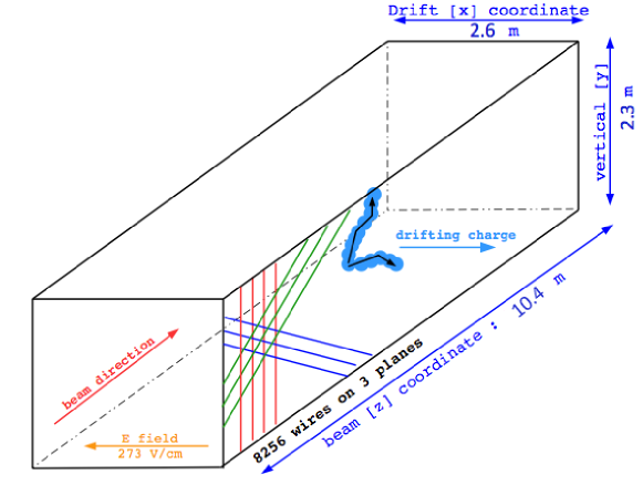
Figure 1: A schematic of the MicroBooNE TPC showing the coordinate system and wire planes.

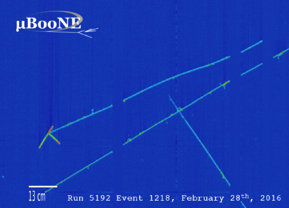
Figure 2: Event display showing raw data for a region of the collection plane associated with a candidate high-multiplicity neutrino event. Wire-number is represented on the horizontal axis, and time on the vertical. Color is associated with the charge deposition on each wire.

The MicroBooNE TPC has an active mass of about 90 tons of liquid argon. It is 10.4 meters long in the beam direction, 2.3 meters tall, and 2.6 meters in the electron drift direction. Electrons require 2.3 ms to drift across the full width of the TPC at the -70 kV operating voltage. Events are read out on three anode wire planes with 3 mm spacing between wires. Drifting electrons pass through the first two wire planes, which are oriented at $\pm 60$ degrees relative to vertical, producing bipolar induction signals.  The third “collection plane” (CP) has its wires oriented vertically and collects the charge of the drifting electrons in the form of a unipolar signal.  The MicroBooNE readout electronics allow for measurement of both the time and charge created by drifting electrons on each wire.

While all three anode planes are used for track reconstruction, the CP provides the best signal-to-noise performance and charge resolution.  The analysis presented here excludes regions of the detector that have non-functional CP channels. It also imposes requirements on the minimum number of CP hits$-$electric current pulses processed through noise filtering  [7], deconvolution, and calibration operations$-$ associated with the reconstructed tracks. All charged particle track candidates are required to have at least 20 CP hits, and the longest muon track candidate is required to have at least 80 CP hits.  Furthermore, as described in Sec. 5, we use two discriminants to extract the neutrino interaction and cosmic ray background contributions to our data sample that are based on CP hits.

A light collection system consisting of 32 8-inch photomultiplier tubes with nanosecond timing resolution enables precise determination of the initial time of the neutrino interaction, which crucially aids in the reduction of cosmic ray backgrounds.

The BNB employs protons from the Fermilab Booster synchrotron impinging on a beryllium target. The proton beam has a kinetic energy of 8 GeV, a repetition rate of up to 5 Hz, and is capable of producing $5\times 10^{12}$ protons-per-spill. Secondary pions and kaons decay producing neutrinos with an average energy of $800$ MeV. The estimated BNB flux is shown in Fig. 3. MicroBooNE received $3.6\times 10^{20}$ protons-on-target in its first year of running from fall 2015 through summer 2016.  This analysis uses a fraction of that data corresponding to $5.0\times 10^{19}$ protons-on-target.

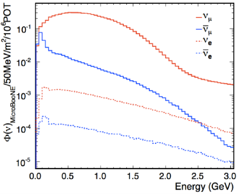
Figure 3: Booster Neutrino Beam flux at the MicroBooNE location for each neutrino flavor.

2 Data and Simulation Samples

2.1 Data

This analysis uses two data samples:

• The “on-beam data”, which is taken only during periods when a beam spill from the BNB is actually sent. The on-beam data used were recorded from February to April 2016 using data taken in runs in which the BNB and all detector systems functioned well [8].  This sample comprises about $15\%$ of the total neutrino data collected by MicroBooNE in its first running period.  The remaining data will be added in the future.

• The “off-beam data”, which is taken with the exact same trigger settings as the on-beam data, but during periods when no beam was received. The off-beam data were collected from February to October 2016.

2.2 Simulation

The LArSoft software framework [9] is used for processing data events and Monte Carlo simulation events in the same way. Five simulation samples are used in this analysis:

• Neutrino interactions generated with default GENIE (“BNB-only MC”).

• CORSIKA [10] cosmic ray (CR) simulation (“CR-only MC”).

• Neutrino interactions simulated with a default GENIE model overlaid with CORSIKA CR events (“BNB+Cosmic default MC”).

• BNB+Cosmic generated with the GENIE implementation of the Meson Exchange Currents model (“BNB+Cosmic with MEC”).

• BNB+Cosmic with the GENIE implementation of the Transverse Enhancement Model (“BNB+Cosmic with TEM”).

The generator stage employs GENIE version 2.8.6 [5] with overlaid simulated CR backgrounds using CORSIKA version v7.4003 [10]. Simulated secondary particle propagation utilizes GEANT version v4.9.6.p04d [6], and detector response simulation employs LArSoft version v4.36.00. All GENIE samples were processed with the same GEANT and LArSoft versions for detector simulation and reconstruction. These samples thus allow for relative comparison of different GENIE models to the data.

3 Event Selection and Signal Extraction

In this analysis, an event selection starts by applying a filter algorithm (“$\nu_{\mu}$ CC filter”) that selects $\nu_{\mu}$ candidates [11]. A set of conditions are then applied to ensure a high quality muon track candidate (“good track filter”). Finally, a “muon directionality classifier” is implemented that categorizes the final selected events into four sub-samples for the purpose of CR background estimation.

3.1 $\nu_{\mu}$ CC Filter

This filter requires events to contain a track candidate that has a minimum reconstructed length of 75 cm that is fully contained within the fiducial volume of the detector.  The light associated with the track candidate must arrive in time coincidence with the beam spill time window, and the candidate must generate a pattern of PMT hits consistent with those expected for a muon track produced in coincidence with the beam arrival. Further details of this selection can be found in Ref. [11]. Considerable CR backgrounds remain after this first stage filter, with signal/background $\simeq$ 1/1. Simple CR background subtraction techniques prove to be insufficient. Later sections describe a new method developed for this analysis to extract neutrino interaction contributions to the observed CPMD.

3.2 Good Track Filter

Pre-selected events then pass through another filter that imposes further quality conditions on track candidates. Start and end points of the candidate muon must lie in detector regions with well-functioning CP wires. Furthermore, the candidate muon track must have at least 80 hits in the collection wire plane, and it must not have significant wire gaps in the start and end 20 CP-hit segments used in the pulse height (PH) test (Sec. 3.3.1) and the multiple Coulomb scattering (MCS) test (Section 3.3.2).

Events passing the $\nu_{\mu}$ CC filter and the good data filter comprise the final data sample. Table 1 lists the event passing rates for the on-beam data, off-beam data, and the BNB+Cosmic MC samples at different steps of the event selection.

Table 1: Passing rates for event selection criteria applied to on-beam data, off-beam data, and BNB+Cosmic MC samples. Numbers are absolute event counts. Quantities in parentheses give the relative passing rate with respect to the step before (first percentage) and the absolute passing rate with respect to the starting sample (second percentage).

	On-beam Data		Off-beam Data		BNB+Cosmic Default MC
Selection Cuts	events	passing rates	events	passing rates	events	passing rates
Generated events	547,616		2,954,586		188,880
$\nu_{\mu}$ CC filtered events	4075	(0.7%/0.7%)	14340	(0.5%/0.5%)	7106	(3.8%/3.8%)
Events passing dead region cut	2577	(63.2%/0.5%)	8206	(57.2%/0.3%)	4993	(70.3%/2.6%)
Events with $\geq 80$ CP hits	2059	(80.0%/0.4%)	5608	(68.3%/0.2%)	4591	(91.9%/2.4%)
Events passing segments gap cuts	1921	(93.3%/0.4%)	5267	(93.9%/0.2%)	4209	(91.7%/2.2%)

3.3 Muon Directionality Classifier

Events satisfying all of the selection criteria are further categorized into the four sub samples based on whether they pass or fail the PH test and the MCS tests described below. These are the tests of the direction of the candidate muon that can be used to separate neutrino signal and CR background contributions in the sample. Table 2 lists the event selection rates for the on-beam data, off-beam data, and the BNB+Cosmic default MC samples in each sub sample.

Table 2: Final event samples from the on-beam data, off-beam data, and BNB+Cosmic MC samples. Numbers are absolute event counts. The percentages correspond to the fraction of events in each test category.

Sub samples	On-beam Data		Off-beam Data		BNB+Cosmic Default MC
PH, MCS	events	acceptance rates	events	acceptance rates	events	acceptance rates
pass, pass	847	(44%)	1263	(24%)	2629	(62%)
pass, fail	367	(19%)	1087	(21%)	737	(18%)
fail, pass	321	(17%)	1141	(22%)	440	(10%)
fail, fail	386	(20%)	1776	(34%)	403	(10%)

3.3.1 Pulse Height Test

A neutrino-induced muon from a CC event will create a track that usually travels in the beam direction (“upstream” to “downstream”) and has an increasing rate of energy loss as one moves downstream along the track.  Selection criteria can be applied to pick tracks that satisfy this expectation in order to suppress cosmic backgrounds.

We take into account the expected behavior of the rate of restricted energy loss [12], $dE/dx_{R}$, with the following procedure:

• Compute the truncated mean of the charge deposited in $20$ consecutive CP hits, $\left\langle PH\right\rangle_{U}$, starting $10$ hits away from the upstream end of the muon track that is taken as a proxy for the upstream restricted energy loss.  The truncated mean is formed by taking the average of the $20$ PH after removing individual PH that do not lie within the range of $20\%-200\%$ of the average [13]:

  $$\left\langle PH\right\rangle_{U}=\frac{\sum\limits_{n=11}^{n=30}PH_{n}\left(0.2\left\langle PH\right\rangle<PH_{n}<2.0\left\langle PH\right\rangle\right)}{\sum\limits_{n=11}^{n=30}\left(0.2\left\langle PH\right\rangle<PH_{n}<2.0\left\langle PH\right\rangle\right)},$$ (3)

  which can be determined iteratively with an initial approximation that $\left\langle PH\right\rangle$ is the arithmetic average.  Use of the truncated mean PH rather than the average PH minimizes effects of large energy loss fluctuations.

• Form a similar quantity from $20$ consecutive CP hits that end 10 CP hits away from the downstream end of the track, $\left\langle PH\right\rangle_{D}$.

• Form the test $p=\left\langle PH\right\rangle_{U}<\left\langle PH\right\rangle_{D}$.  Muons from $\nu_{\mu}$ CC interactions will pass this test with a probability $P\left(PH\right)$.  Muons from CR background can be characterized by the probability that they fail the negation of the test $\bar{p}=\left\langle PH\right\rangle_{U}>\left\langle PH\right\rangle_{D}$, denoted as $Q\left(PH\right).$

A visual diagram for the PH test is shown in Figure 4. Figure 5 presents the pulse height downstream to upstream ratio distribution for BNB+Cosmic default MC (signal+cosmic background) and off-beam data (cosmic background only). We observe that PH ratio for the signal significantly dominates over the background for values $>$1, which was the cut value chosen for the signal-enhanced sample used in the analysis.

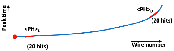
Figure 4: Diagram showing PH test for a candidate muon track.

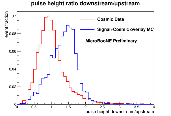
Figure 5: Pulse height (PH) downstream to upstream ratio $\left\langle PH\right\rangle_{D}/\left\langle PH\right\rangle_{U}$.

3.3.2 MCS Test

A neutrino-induced muon from a CC event will create a track that usually travels in the beam direction (“upstream” to “downstream”) and has an increasing degree of scatter about a nominal straight line trajectory as one moves downstream along the track.  Selection criteria can be applied to pick tracks that satisfy this expectation in order to suppress cosmic backgrounds.

The expected MCS behavior is taken into account by an independent test with the following procedure:

• Take three 20 CP-hit long track segments at the upstream, downstream, and geometric center of the track.  The upstream and downstream segments are displaced by 10 CP hits from the upstream and downstream ends of the track, respectively.

• Perform a simple linear least squares fit of hit time vs. (wire) position using the $20$ contiguous CP hits at the upstream end of the track.  Denote the determined line as $L_{U}$. Perform a similar fit using the $20$ CP hits at the downstream end of the track.  Denote the determined line as $L_{D}.$ Finally perform one more similar fit from the $20$ CP hits located about the geometric center of the track. Denote this line as $L_{M}$.

• Compare the hit time (drift direction ‘$x$’) predicted at the geometric center of the track, $t_{C}$, by $L_{M}$, which uses hits about the geometric center, to the time predicted at the geometric center of the track by the projection of $L_{U}$ from the beginning of the track:

  $$\Delta t_{UM}=\left|t_{C}\left(L_{U}\right)-t_{C}\left(L_{M}\right)\right|.$$ (4)

• Repeat the process except compare $t_{C}$ from $L_{M}$ to the time predicted at the geometric center of the track by the projection of $L_{D}$ from the end of the track:

  $$\Delta t_{DM}=\left|t_{C}\left(L_{D}\right)-t_{C}\left(L_{M}\right)\right|.$$ (5)

• Form the test $q=\Delta t_{UM}<\Delta t_{DM}$.  Since MCS should become, on average, more pronounced along the downstream end of the track as the momentum decreases, this provides a second directional test on the muon track candidate.  Muons from $\nu_{\mu}$ CC interactions will pass this test with a probability $P\left(MCS\right)$.  Muons from CR background tests can be characterized by the probability that they fail the negation of the test $\bar{q}=\Delta t_{UM}>\Delta t_{DM}$, denoted as $Q\left(MCS\right).$

A visual diagram for the MCS test is shown in Figure 6. Figure 7 presents the MCS downstream to upstream ratio $\Delta t_{DM}/\Delta t_{UM}$ distribution for BNB+Cosmic default MC (signal+cosmic background) and off-beam data (cosmic background only). We observe that MCS ratio for the signal dominates over the background for values $>$1, which was the cut value chosen for the signal-enhanced sample used in the analysis.

Figure 6: Diagram of MCS directionality test for a candidate muon track.

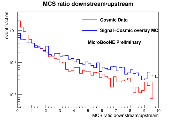
Figure 7: Multiple Coulomb scattering (MCS) downstream to upstream ratio $\Delta t_{DM}/\Delta t_{UM}$.

4 Expectations for Observed Charged Particle Multiplicity Distribution 

All $\nu_{\mu}$ CC events inherently have a muon and at least one charged hadron at the initial neutrino interaction vertex. In order to mitigate backgrounds from cosmic ray (CR) interactions, which are significant due MicroBooNE’s placement at the earth’s surface, muon track candidates must produce a visible track with a physical length of at least 75 cm in argon that has all its TPC hits contained within a detector fiducial volume defined to be the liquid argon volume within the TPC that is greater than 5 cm from any TPC boundary.  The candidate muon containment requirement limits its energy to be $\lesssim 1.2$ GeV depending on the muon scattering angle. This results in a sample biased towards relatively higher inelasticity $y=\nu/E_{\nu}$, in the rest frame of the hadronic system, with $\nu$ the energy transferred from the neutrino to the hadronic system in the collision.

At BNB energies, the nominally dominant charged particle multiplicities at the neutrino interaction point are $\mathcal{O}\left(80\%\right)$ $n=2$ (from quasi-elastic scattering, $\nu_{\mu}n\rightarrow\mu^{-}p$, neutral pion resonant production $\nu_{\mu}n\rightarrow\mu^{-}R^{+}\rightarrow\mu^{-}p\pi^{0}$, and coherent pion production $\nu_{\mu}\mathrm{Ar}\rightarrow\mu^{-}\pi^{+}\mathrm{Ar}$), $\mathcal{O}\left(20\%\right)$ $n=3$ (resonant  charged pion production $\nu_{\mu}p\rightarrow\mu^{-}R^{++}\rightarrow\mu^{-}p\pi^{+}$), and $\mathcal{O}\left(1\%\right)$ $n\geq 4$ (from multiparticle production processes referred to as “deep inelastic scattering”(DIS)).  However final state interactions (FSI) of hadrons produced in neutrino scattering with the argon nucleus can subtract or add charged particles that emerge from within the nucleus. These multiplicities are further modified by the selection cuts.

We require tracks to register a minimum number of CP hits $(20)$ in the TPC so that the Pandora MicroBooNE track reconstruction algorithms [14] operate optimally. Tracks with less than $20$ CP hits may fail to reconstruct due to inefficiencies in the reconstruction algorithms. This minimum CP hit condition corresponds to a minimum range in liquid argon of 6 cm, and the requirement thus excludes charged particles below a particle-type-dependent kinetic energy threshold from entering our sample. This threshold ranges from $37$ MeV for a $\pi^{\pm}$ to $82$ MeV for a proton, and this measurement has no acceptance for particles with kinetic energies below these thresholds. These thresholds are also dependent on the angle of the track with respect to the collection plane wires.

The average MicroBooNE charged track reconstruction efficiency is $\left\langle\epsilon\right\rangle\approx 45\%$ [15] at the $20$ hits threshold used in this analysis.  This relatively low value, with implicit kinetic energy thresholds, creates a common occurrence called “feed-down” wherein events produced with $n$ tracks at the argon nucleus exit position are reconstructed with an observed multiplicity $n^{\prime}<n$.  For example, $n=1$ is commonly observed because one of the two tracks in a quasi-elastic event fails to be reconstructed.

The underlying observed CPMD in MicroBooNE is expected to lie predominantly in the $n=1-4$ range.  The following summarizes qualitative expectations for components of observed multiplicities from particular processes.  These components can include contributions from the primary neutrino-nucleon scatter within the nucleus and secondary interactions of primary hadrons with the remanent nucleus.  Secondary charged particles are usually protons, which are expected to be produced with kinetic energies that are usually too low for track reconstruction in this analysis.  However, more energetic forward-produced protons from the upper “tail” of this secondary kinetic energy distribution may make it into our sample.

• Multiplicity $>3$, mainly predicted to be “DIS events” in which at least three short tracks are reconstructed.  “DIS” is the usual term for multiparticle final states not identified with any particular resonance formation.  Some contribution could exist from multiplicity=3 resonant charged pion production accompanied by a proton from the high-energy tail of the final state interaction proton production distribution.

• Multiplicity $=3$, mainly predicted to be $\mu^{-}p\pi^{+}$ events from $\Delta$ resonance production in which all three tracks are reconstructed.  “Feed down” from higher multiplicity would be small due to the tiny DIS cross section at MicroBooNE energies.  Some contribution could exist from multiplicity=2 QE scattering accompanied by a proton from the high-energy tail of the final state interaction proton production distribution.

• Multiplicity $=2$, mainly predicted to be QE $\mu^{-}p$ events in which the proton is reconstructed, with a sub-leading contribution from “feed down” of resonant charged pion production events where one track fails to be reconstructed.  Multiplicity 2 could be augmented by high energy final state interaction protons.

• Multiplicity $=1$, mainly predicted to be “feed down” from QE $\mu^{-}p$ and $\mu^{-}p\pi^{0}$ events in which the proton is not reconstructed, with contributions from other higher multiplicity topologies in which more than one tracks fails to be reconstructed.

Figure 8 illustrates these expectations using our BNB-only MC simulation. The $O_{2}/O_{1}$ ratio may be sensitive to the proton kinematics from QE scattering.  The $O_{3}/O_{2}$ ratio may provide sensitivity to the value of the $\Delta$ resonance production cross section relative to the QE cross section and to the pion kinematics from resonance decay and propagation through the nucleus.  Higher $n$ values of $O_{n}$ could test for the DIS contribution and the presence of high energy tails in proton production by final state interactions (FSI).

We note that our kinetic energy thresholds limit acceptance in such a way that protons produced in FSI may not significantly contribute to the observed CPMD. Furthermore, our analysis requires a forward-going long contained track as a muon candidate, which restricts the final state phase space.  Our results should therefore not be compared to the low energy proton multiplicity measurement reported by ArgoNeuT [16].  A future publication will be devoted to a measurement of proton multiplicity in MicroBooNE over a larger phase space.

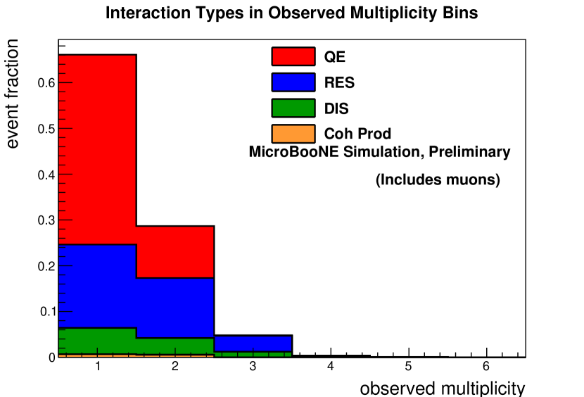
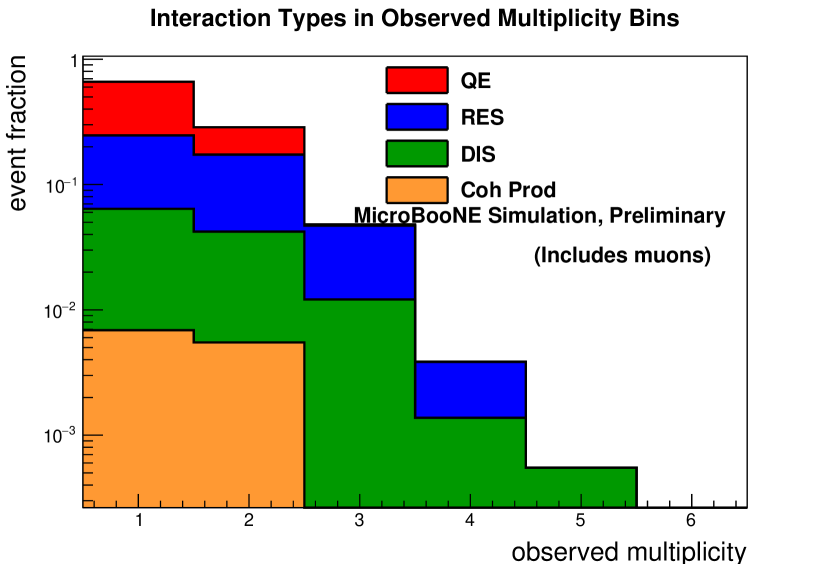
Figure 8: Observed (stacked) multiplicity distributions for different neutrino interaction types from our BNB-only default MC simulation in linear scale (left) and in log y scale (right).

5 Analysis Method and Results

5.1 Cosmic ray Backgrounds in MicroBooNE

The MicroBooNE detector lacks appreciable shielding from cosmic rays.  Most events that pass trigger conditions during neutrino beam operations (“on-beam data”) contain no neutrino interactions, and triggered events with a neutrino interaction typically have the products of several cosmic rays in the event readout window contributing to the detector response along with the products of the neutrino collision.  A large sample of events recorded under identical conditions as the on-beam data, except for the coincidence requirement with the beam, (“off-beam-data”) has been recorded for use in characterizing CR backgrounds.  A straightforward on-beam minus off-beam background subtraction is, however, difficult, as the off-beam data does not reproduce all correlated detector effects associated with on-beam events containing a neutrino interaction with several overlaid cosmic rays.  The situation is particularly complicated with observed multiplicity$=$1 neutrino interaction events, which share a common topology with the abundant single muon CR background MC simulations of the CR flux using the CORSIKA package provide useful guidance; however, the ability of these simulations to describe the very rare CR topologies that closely match neutrino interactions is not yet well understood.

For these reasons, this analysis employs a method to separate neutrino interaction candidates from CR backgrounds that is driven by the data itself.  The separation rests on the observation that a neutrino $\nu_{\mu}$ CC interaction produces a final state $\mu^{-}$ that slows down as it moves away from its production point at the neutrino interaction vertex due to ionization energy loss in the liquid argon.  As it slows down, its rate of restricted energy loss, $dE/dx_{R}$, increases, and deviations from a linear trajectory due to multiple Coulomb scattering (MCS) become more pronounced.  A CR muon track can produce an apparent neutrino interaction vertex if it comes to rest in the detector, but the CR track will exhibit large $dE/dx_{R}$ and MCS effects in the vicinity of this vertex.  Furthermore, the vast majority of $\nu_{\mu}$ CC muons that satisfy the $75$ cm length requirement travel in the neutrino beam direction (“upstream” to “downstream”), whereas CR muons move upstream or downstream with equal probability.

5.2 Data-Driven Signal+Background Model

On-beam data consists of a mixture of neutrino interaction and CR background events.  For each observed track multiplicity, we divide the data sample into four data categories, denoted as “$\nu\nu$”, “$CR\nu$”, “$\nu CR$”, and “$CRCR$” according to the outcome of the PH and MCS tests performed on the longest track in the event.  These samples contain numbers of events equal to $N_{\nu\nu}$, $N_{CR\nu}$, $N_{\nu CR},$ and $N_{CRCR}$, respectively.  The “$\nu$” designation indicates that the $PH$ or $MCS$ test categorizes the long track as being more likely a $\nu_{\mu}$ CC event candidate muon, while the “$CR$” designation corresponds to a long track candidate falling into the more likely CR class according to the $PH$ or $MCS$ test.  The number of events in each category, for each multiplicity, is then modelled by the following:

$$\hat{N}_{\nu\nu} =P\left(MCS|PH\right)P\left(PH\right)\hat{N}_{\nu}$$ (6)

$$+\left(1-Q\left(PH\right)-Q\left(MCS\right)+Q\left(MCS|PH\right)Q\left(PH\right)\right)\hat{N}_{CR},$$

$$\hat{N}_{CR\nu} =\left(1-P\left(MCS|PH\right)\right)P\left(PH\right)\hat{N}_{\nu}$$ (7)

$$+\left(Q\left(MCS\right)-Q\left(MCS|PH\right)Q\left(PH\right)\right)\hat{N}_{CR},$$

$$\hat{N}_{\nu CR} =\left(P\left(MCS\right)-P\left(MCS|PH\right)P\left(PH\right)\right)\hat{N}_{\nu}$$ (8)

$$+\left(1-Q\left(MCS|PH\right)\right)Q\left(PH\right)\hat{N}_{CR},$$

$$\hat{N}_{CRCR} =\left(1-P\left(PH\right)-P\left(MCS\right)+P\left(MCS|PH\right)P\left(PH\right)\right)\hat{N}_{\nu}$$ (9)

$$+Q\left(MCS|PH\right)Q\left(PH\right)\hat{N}_{CR},$$

where $\hat{N}_{\nu\nu}$ corresponds to the number of event in the sample that passes both PH and MCS tests and $\hat{N}_{CRCR}$ corresponds to the number of events in the sample that fails both PH and MCS tests. These are expected to be the samples with enriched neutrino and CR content, respectively, $\hat{N}_{CR\nu}$ and $\hat{N}_{\nu CR}$ corresponds to the number of events in the sample that pass one test and fails the other. These are the samples of mixed purity.  The quantities $\hat{N}_{\nu}$ and $\hat{N}_{CR}$ are the to-be-fitted number of neutrino and CR events, respectively, in the sample.

The conditional probability $P\left(MCS|PH\right)$ denotes the fraction of time that an event passes the $MCS$ condition after it has passed the $PH$ condition.  As the $MCS$ and $PH$ conditions result from different physical processes (muon-nucleus and muon-electron scattering, respectively) and the $MCS$ and $PH$ test are formed primarily from different quantities (time and charge, respectively), the PH and MCS tests are nearly independent, $P\left(MCS|PH\right)\approx$ $P\left(MCS\right)$.  In the analysis we find evidence for weak correlations between the tests, and use of the conditional probability allows for this to be taken into account.

Off-beam data, which contains no neutrino content, is divided into the same categories, with event counts $N_{\nu\nu}^{\prime}$, $N_{CR\nu}^{\prime}$, $N_{\nu CR}^{\prime},$ and $N_{CRCR}^{\prime}$, and modeled as

$$\hat{N}_{\nu\nu}^{\prime} =\left(1-Q\left(PH\right)-Q\left(MCS\right)+Q\left(MCS|PH\right)Q\left(PH\right)\right)\hat{N}_{CR}^{\prime},$$ (10)

$$\hat{N}_{CR\nu}^{\prime} =\left(Q\left(MCS\right)-Q\left(MCS|PH\right)Q\left(PH\right)\right)\hat{N}_{CR}^{\prime},$$ (11)

$$\hat{N}_{\nu CR}^{\prime} =\left(1-Q\left(MCS|PH\right)\right)Q\left(PH\right)\hat{N}_{CR}^{\prime},$$ (12)

$$\hat{N}_{CRCR}^{\prime} =Q\left(MCS|PH\right)Q\left(PH\right)\hat{N}_{CR}^{\prime}.$$ (13)

where $\hat{N}_{\nu\nu}^{\prime}$ and $\hat{N}_{CRCR}^{\prime}$ are expected to be enriched samples containing muons characteristic of neutrino interactions and cosmic rays, respectively, and $\hat{N}_{CR\nu}^{\prime}$ and $\hat{N}_{\nu CR}^{\prime}$ are samples of mixed purity; and  $\hat{N}_{CR}^{\prime}$ is the to-be-fitted CR content of the sample (in practice the number of events in the sample).

Two parameters, $\alpha_{\nu}$and $\alpha_{\text{CR}}$ describe the conditional probabilities $P\left(MCS|PH\right)$ and $Q\left(MCS|PH\right)$ via the parameterizations given below. These are calculated from the BNB-only MC simulation and off-beam data, respectively.  These are parameterized as

$$P\left(MCS|PH\right) =\frac{\alpha_{\nu}P\left(MCS\right)}{1+\left(\alpha_{\nu}-1\right)P\left(MCS\right)},$$ (14)

$$Q\left(MCS|PH\right) =\frac{\alpha_{\text{CR}}Q\left(MCS\right)}{1+\left(\alpha_{\text{CR}}-1\right)Q\left(MCS\right)}.$$ (15)

Our algorithm uses the eight categories of events (Eqs. 6-13) in on-beam and off-beam data to fit for the neutrino content in each observed multiplicity bin.

5.3 Fitting Procedure

We construct a likelihood function based on the probability distribution for partitioning events into one of four categories, a multinomial distribution.  The multinomial probability of observing $n_{i}$ events in bin $i$, with $i=1,2,3,4$, with the probability of a single event landing in bin $i$ equal to $r_{i}$ is

$$M\left(n_{1},n_{2},n_{3},n_{4};r_{1},r_{2},r_{3},r_{4}\right)=\frac{\left(n_{1}+n_{2}+n_{3}+n_{4}\right)!}{n_{1}!n_{2}!n_{3}!n_{4}!}r_{1}^{n_{1}}r_{2}^{n_{2}}r_{3}^{n3}r_{4}^{n_{4}}.$$ (16)

The $n_{i}$ will be the observed number of events in each multiplicity bin, and the $r_{i}$ will be functions of the model fit parameters:

on-beam: $$M\left(N_{\nu\nu},N_{CR\nu},N_{\nu CR},N_{CRCR};\frac{\hat{N}_{\nu\nu}}{\hat{N}},\frac{\hat{N}_{CR\nu}}{\hat{N}},\frac{\hat{N}_{\nu CR}}{\hat{N}},\frac{\hat{N}_{CRCR}}{\hat{N}}\right),$$ (17)

off-beam: $$M\left(N_{\nu\nu}^{\prime},N_{CR\nu}^{\prime},N_{\nu CR}^{\prime},N_{CRCR}^{\prime};\frac{\hat{N}_{\nu\nu}^{\prime}}{\hat{N}^{\prime}},\frac{\hat{N}_{CR\nu}^{\prime}}{\hat{N}^{\prime}},\frac{\hat{N}_{\nu CR}^{\prime}}{\hat{N}^{\prime}},\frac{\hat{N}_{CRCR}^{\prime}}{\hat{N}^{\prime}}\right),$$ (18)

with

$$\hat{N} =\hat{N}_{\nu\nu}+\hat{N}_{CR\nu}+\hat{N}_{\nu CR}+\hat{N}_{CRCR},$$ (19)

$$\hat{N}^{\prime} =\hat{N}_{\nu\nu}^{\prime}+\hat{N}_{CR\nu}^{\prime}+\hat{N}_{\nu CR}^{\prime}+\hat{N}_{CRCR}^{\prime}.$$ (20)

The likelihood also incorporates the Poisson statistics of observing $n_{1}+n_{2}+n_{3}+n_{4}$ in both the on-beam and off-beam data:

on-beam: $$\frac{\hat{N}^{N}}{N!}e^{-\hat{N}},$$ (21)

off-beam: $$\frac{\hat{N}^{\prime N^{\prime}}}{N^{\prime}!}e^{-\hat{N}^{\prime}},$$ (22)

with

$$N =N_{\nu\nu}+N_{CR\nu}+N_{\nu CR}+N_{CRCR},$$ (23)

$$N^{\prime} =N_{\nu\nu}^{\prime}+N_{CR\nu}^{\prime}+N_{\nu CR}^{\prime}+N_{CRCR}^{\prime}.$$ (24)

The final likelihood function is

$$L_{TOT} =M\left(N_{\nu\nu},N_{CR\nu},N_{\nu CR},N_{CRCR};\frac{\hat{N}_{\nu\nu}}{\hat{N}},\frac{\hat{N}_{CR\nu}}{\hat{N}},\frac{\hat{N}_{\nu CR}}{\hat{N}},\frac{\hat{N}_{CRCR}}{\hat{N}}\right)$$ (25)

$$\times M\left(N_{\nu\nu}^{\prime},N_{CR\nu}^{\prime},N_{\nu CR}^{\prime},N_{CRCR}^{\prime};\frac{\hat{N}_{\nu\nu}^{\prime}}{\hat{N}^{\prime}},\frac{\hat{N}_{CR\nu}^{\prime}}{\hat{N}^{\prime}},\frac{\hat{N}_{\nu CR}^{\prime}}{\hat{N}^{\prime}},\frac{\hat{N}_{CRCR}^{\prime}}{\hat{N}^{\prime}}\right)$$

$$\times\frac{\hat{N}^{N}}{N!}e^{-\hat{N}}\times\frac{\hat{N}^{\prime N^{\prime}}}{N^{\prime}!}e^{-\hat{N}^{\prime}}.$$

The model fit parameters and their statistical uncertainties are estimated via the maximum likelihood method, implemented by minimizing the negative-log-likelihood

$$\mathcal{L}_{TOT}=-\ln L_{TOT}\text{,}$$ (26)

using the MIGRAD minimization in the standard MINUIT [17] package in ROOT [18].

The fitting procedure can be used to obtain estimates for $\hat{N}_{\nu}$, $\hat{N}_{CR}$, $\hat{N}_{CR}^{\prime}$, $P\left(PH\right)$, $P\left(MCS\right)$, $Q\left(PH\right)$, and $Q\left(MCS\right)$ for each multiplicity.  When the probability parameters are consistent between multiplicities, we use all multiplicities together in their determination for improved statistical precision and vary the three parameters $\hat{N}_{\nu}$, $\hat{N}_{CR}$, and $\hat{N}_{CR}^{\prime}$ for each multiplicity.

In total, we have eight equations (Eqs. 6$-$13), where first four come from on-beam data and the other four come from off-beam data. We have nine parameters $\hat{N}_{\nu}$, $\hat{N}_{CR}$, $\hat{N}_{CR}^{\prime}$, $P(PH)$, $Q(PH)$, $P(MCS)$, $Q(MCS)$, $\alpha_{\nu}$ and $\alpha_{CR}$. After proving that the off-beam data and CR-only MC are consistent, the parameters $\alpha_{\nu}$ and $\alpha_{CR}$ were obtained from BNB-only MC simulation and off-beam data samples, respectively, and were kept fixed afterwards. The maximum likelihood fit was performed to obtain the values of the rest of seven parameters from simulation (BNB+Cosmic default MC $\&$ off-beam data) and data (on-beam $\&$ off-beam data) samples.  Figure 9 presents a schematic diagram for the fitting process and also lists the fixed and floating parameters for each fit.

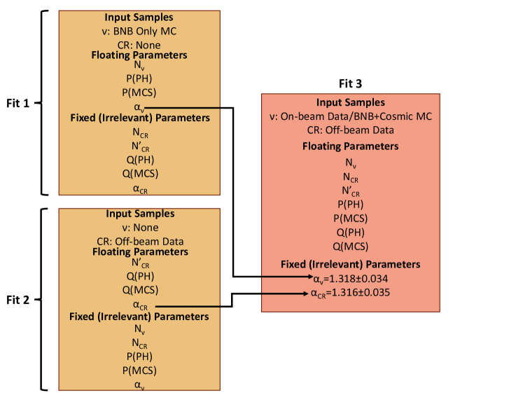
Figure 9: Fitting process diagram. Fixed and floating parameters and input samples are listed for each fit.

5.4 Results on Simulation

A maximum likelihood fit was performed on all three different simulation samples. This fit was performed to extract the values of seven parameters $\hat{N}_{\nu}$, $\hat{N}_{CR}$, $\hat{N}_{CR}^{\prime}$, $P(PH)$, $Q(PH)$, $P(MCS)$, and $Q(MCS)$). As expected, the $PH$ and $MCS$ probabilities show no statistically significant difference between the three GENIE models considered.  Table 3 lists the fit values obtained from the fit for the above-mentioned parameters in the BNB+Cosmic default MC and the off-beam data.

Table 3: Fit parameter results and corresponding errors for the BNB+Cosmic default MC simulation and off-beam data samples as well as the on-beam and off-beam data samples. The same off-beam data sample was used in both fits.  All errors are from the fit and are purely statistical.

	Fit Results
Parameters	BNB+Cosmic MC	MicroBooNE Data
$\hat{N}_{\nu}$	3602$\pm$154	1056$\pm$169
$\hat{N}_{CR}$	607$\pm$144	865$\pm$169
$\hat{N}_{CR}^{\prime}$	5267$\pm$73	5267$\pm$73
$P(PH)$	0.859$\pm$0.017	0.784$\pm$0.052
$P(MCS)$	0.775$\pm$0.012	0.732$\pm$ 0.038
$Q(PH)$	0.554$\pm$0.007	0.554$\pm$0.007
$Q(MCS)$	0.544$\pm$0.007	0.544$\pm$ 0.007

5.5 Closure Test Results

The number of neutrino events in the simulated data samples were extracted and compared to the known number from the event generation. Table 4 and Figure 10 summarize this comparison. We find that fit results agree within statistics with the known inputs, indicating a lack of bias in our signal estimation technique.  We have also verified that our method is insensitive to the signal-to-background ratio of the sample over a range corresponding to $0.2-5.0\$times that estimated in the data.

Table 4: Fitted and true number of neutrino events for the BNB+Cosmic default MC sample for different multiplicity bins. The last column shows good agreement between the fit results and true content for different bins.

Multiplicities	Fit $N_{\nu}$	True $N_{\nu}$	True-Fit $\chi^{2}$/ndf
1	2340$\pm$65	2405	1.0
2	1018$\pm$41	1043	0.4
3	176$\pm$13	175	0.0
4	14$\pm$3	14	0.0
5	2$\pm$1	2	0.0

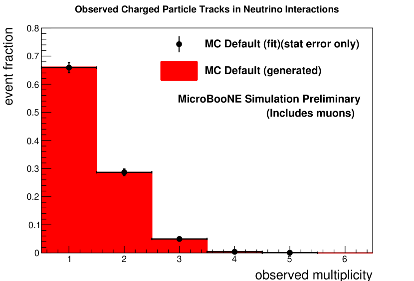
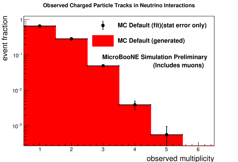
Figure 10: Bin-by-bin fitted, area normalized, and CR-background-subtracted observed neutrino multiplicity distribution from the BNB+Cosmic default MC sample in linear scale (left) and in log y scale (right).

5.6 Statistical and Systematic Uncertainty Estimates

5.6.1 Statistical Uncertainties

Statistical uncertainties are returned from the MINUIT package used in our fitting for both data and MC samples. These uncertainties include contributions from the CR background in our fitting procedure.  Both data and MC statistics contribute substantially to the overall uncertainties in our data, as shown in Figures 11a and 11b. These will be reduced in the future by employing the full MicroBooNE data set from its first run and by generating larger MC samples.

(a)

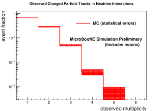
(b)

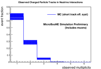
(c)

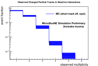
(d)

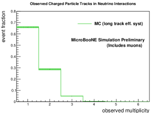
(e)

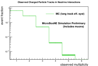
(f)

Figure 11: Systematic uncertainty contributions to observed CPMD due to MC statistics (top row), short track efficiency (middle row), and long track efficiency (bottom row). The width of the line on the histogram indicates the uncertainty band.

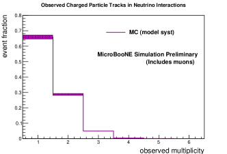
(a)

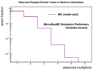
(b)

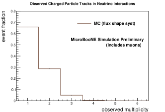
(c)

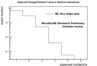
(d)

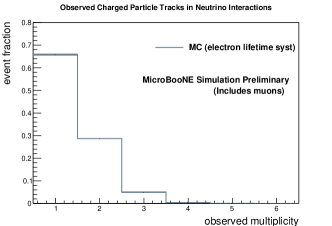
(e)

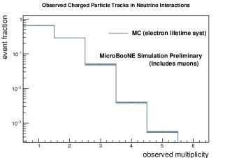
(f)

Figure 12: Systematic uncertainty contributions to observed CPMD due to background model uncertainty (top row), flux (middle row), and electron lifetime (bottom row). The width of the line on the histogram indicates the uncertainty band.

5.6.2 Short Track Efficiency Uncertainties

The dominant systematic uncertainty derives from the analysis of possible differences in the efficiency between data and MC for reconstructing the shorter length hadron tracks. The overall efficiencies of the Pandora reconstruction algorithms [15] are a strong function of the number of hits of the tracks, with plateau not being reached until of order of several hundred hits.  The inclusive efficiencies for reconstructing protons or pions at the 20 CP hit threshold is estimated to be $\left\langle\epsilon\right\rangle=0.45\pm 0.05$.  The absolute efficiency value is not used in this analysis, but we use this estimate to conservatively assign a mean efficiency uncertainty of $\delta=15\%$.

We then estimate the effect of an efficiency uncertainty on multiplicity by the following procedure: Consider a track in an event that has made it into a particular multiplicity bin $N$.  If one lowers the tracking efficiency by the factor $1-\delta$, then there is a 1-$\delta$ probability that the track reconstructed and the event stayed in that multiplicity bin, and a probability $\delta$ that the track would not have been reconstructed and that the event would thus have a lower multiplicity.   If the overall multiplicity is $N$, with $N-1$ short tracks and the one long track, and each track’s reconstruction probability is reduced by a factor $1-\delta$, then an overall fraction of events $\left(1-\delta\right)^{N-1}$ will remain in the bin, and a fraction $1-\left(1-\delta\right)^{N-1}$ will migrate to lower multiplicity bins. The fraction of tracks that migrate to multiplicity $N^{\prime}<N$ from bin $N$, $f\left(N^{\prime};N,\delta\right)$, is given by binomial statistics:

$$f\left(N^{\prime};N,\delta\right)=\frac{\left(N-1\right)!}{\left(N^{\prime}-1\right)!\left(N-N^{\prime}\right)!}\left(1-\delta\right)^{N^{\prime}-1}\delta^{N-N^{\prime}}.$$ (27)

We use this result to generate the expected observed CPMD in simulation that would emerge from lowering the tracking efficiency by the factor $1-\delta$ compared to the default simulated CPMD.  The difference between the two distributions is then taken as the systematic uncertainty assigned to short track efficiency, with the assumption that the effect of increasing the default efficiency by a factor $1+\delta$ would produce a symmetric change. Table 5 summarizes this study for the three GENIE models used.  The observed multiplicity $=1$ bin observed probability increases because of more “feed down” of events from higher multiplicity due to the lowered efficiency, mainly from observed multiplicity $=2$.  The other observed multiplicity probabilities accordingly decrease.  The biggest effects are in high multiplicity bins because the loss of events from lowering the efficiency by the factor $\left(1-\delta\right)$ goes like $\left(1-\delta\right)^{N-1}$ for multiplicity bin $N$.  The estimates do not consider the possibility of “fake tracks” that could move events to higher multiplicity. Figure 11c and 11d present the short track efficiency error bands on the default simulation.

Table 5: Relative change in observed multiplicity probabilities corresponding to a -15% uniform reduction in short charged particle tracking efficiencies for three GENIE models: default, MEC, and TEM. The missing entry for multiplicity 5 in TEM is due to no event being generated with that multiplicity.

Observed multiplicity	$\frac{\Delta P_{n}}{P_{n}}$Default	$\frac{\Delta P_{n}}{P_{n}}$MEC	$\frac{\Delta P_{n}}{P_{n}}$TEM
$1$	$+7\%$	$+7\%$	$+8\%$
$2$	$-11\%$	$-12\%$	$-12\%$
$3$	$-25\%$	$-25\%$	$-25\%$
$4$	$-33\%$	$-36\%$	$-39\%$
$5$	$-44\%$	$-48\%$	–

5.6.3 Long Track Efficiency Uncertainties

To first order, the efficiency for reconstructing the $>75$ cm length track used to define the sample would not be expected to affect the observed multiplicity distribution, as it is common to all multiplicities and cancels in the ratio to form observed multiplicity probabilities.  At second order, however, a multiplicity dependence could come in that changes the distribution of observed multiplicity without affecting the overall number of events.  A plausible model for this is that higher multiplicity in an event helps Pandora better define a vertex, and thus helps the event pass the $\nu_{\mu}$ CC selection filter.

We estimate the size of this effect by comparing the efficiencies obtained with the Pandora package [15] to simulated quasi-elastic final states in which both the proton and muon are reconstructed to charged pion resonance final states in which the proton, pion, and muon are all reconstructed.  From this study we conclude that the efficiency for finding the muon in final states where all charged particles are reconstructed could be up to $3\%$ higher for charged pion resonance events (observed multiplicity 3) than quasi-elastic events (observed multiplicity 2). We then assume, for the purpose of uncertainty estimation, that this relative enhancement seen for higher observed multiplicity events in the MC is completely absent in the data.

Table 6 summarizes this study.  Effects are generally small compared to those seen in Table 5.  No dependence on GENIE version is found. Figure 11e and 11f present the long track efficiency error bands on the default simulation.

Table 6: Relative change in observed multiplicity probabilities corresponding to increasing the conditional probability for reconstructing the long track by 3% for each additional track found in the event, as suggested by Pandora studies of QE and charged pion resonance production for three GENIE models: default, MEC, and TEM. The missing entry for multiplicity 5 in TEM is due to no event being generated with that multiplicity.

Observed multiplicity	$\frac{\Delta P_{n}}{P_{n}}$Default	$\frac{\Delta P_{n}}{P_{n}}$MEC	$\frac{\Delta P_{n}}{P_{n}}$TEM
$1$	$-1\%$	$-1\%$	$-1\%$
$2$	$+2\%$	$+2\%$	$+2\%$
$3$	$+4\%$	$+4\%$	$+2\%$
$4$	$+7\%$	$+7\%$	$+7\%$
$5$	$+9\%$	$+9\%$	–

5.6.4 Background Model Uncertainties

In the signal extraction fitting procedure, two conditional parameters ($\alpha_{\nu}$ and $\alpha_{CR}$) were extracted from Monte Carlo simulation and the off-beam data and were kept fixed afterwards. To calculate the systematic uncertainties on these parameters, their values were varied $\pm 1\sigma$ of their statistical errors. Those values were propagated in the observed charged particle multiplicity distribution and the resulting distributions are shown in Figures 12a and 12b. The effect of this systematic was found to be very small. The systematic errors obtained from different multiplicity bins were added in quadrature in the final observed charged particle multiplicity distribution.

5.6.5 Flux Shape Uncertainties

Variations in flux can be parameterized by

$$\Phi\left(E_{\nu}\right)\rightarrow\left(1+\delta\left(E_{\nu}\right)\right)\Phi\left(E_{\nu}\right),$$ (28)

where $\Phi\left(E_{\nu}\right)$ is the neutrino flux at neutrino energy $E_{\nu}$ and $\delta\left(E_{\nu}\right)$ is the fractional uncertainty in the flux at that energy. An energy-independent $\delta\left(E_{\nu}\right)$ would have no effect on observed multiplicity distributions as this measurement is independent of absolute normalization.  On the other hand, shifts that, for example, raise the high energy flux relative the low energy flux could in principle enhance the contributions of higher multiplicity resonance and DIS processes. We confine ourself to considering highly correlated energy-dependent shifts, denoted as $\delta_{i}\left(E_{\nu}\right)$ for $i=1-6$ via an approximate procedure that should be conservative.  These shifts, shown in Figure 13 are allowed to modify the BNB flux within uncertainties determined by the MiniBooNE collaboration [2].  The first two variations simply shift all flux values up ($\delta_{1}\left(E_{\nu}\right)$) or down ($\delta_{2}\left(E_{\nu}\right)$) together according to the flux uncertainty envelope.  The next two relatively enhance high energy flux ($\delta_{3}\left(E_{\nu}\right)$) or low energy flux ($\delta_{4}\left(E_{\nu}\right)$) linearly with neutrino energy, with the variation taken to be zero at the average energy.  The final two relatively enhance high energy flux ($\delta_{5}\left(E_{\nu}\right)$) or low energy flux ($\delta_{6}\left(E_{\nu}\right)$) logarithmically with neutrino energy, with the variation taken to be zero at the average energy. As expected, shifts that are positively correlated across all energies produce negligible differences, but even shifts that produce sizable distortions between high and low energies contribute a systematic uncertainty contribution that is small. Figure 12c and 12d present the flux systematic error bands on the default simulation.

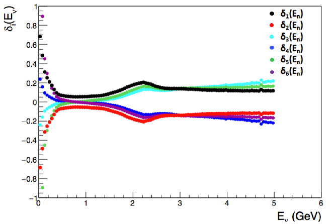
Figure 13: Beam flux shifts for the parameterizations $\delta_{i}\left(E_{\nu}\right)$, $i=1-6$.  The variations $\delta_{1}\left(E_{\nu}\right)$ and $\delta_{2}\left(E_{\nu}\right)$ define the envelope of flux uncertainties for the BNB.

5.6.6 Electron Lifetime Uncertainties

The measured charge from muon-induced ionization can vary over the detector volume due to the finite probability for drifting electrons to be captured by electronegative contaminants in the liquid argon.  This capture probability can be parameterized by an electron lifetime $\tau$. We perform our analysis on simulated data with two lifetimes that safely bound those found during data taking detector operation conditions, $\tau=$ 6 msec and $\tau=\infty$ msec .  Figures 12e and 12f show the result that electron lifetime uncertainties minimally affect this analysis.

5.6.7 Other Sources of Uncertainty

A systemic comparison was performed of all kinematic quantities entering this analysis between off-beam CR data and the CR events simulated with CORSIKA. No statistically significant discrepancies were observed between event selection pass rates applied to off-beam data vs. MC simulation.

A check of possible time-dependent detector response systematics was also performed by dividing the on-beam data into two samples and performing the analysis separately for each sample. Differences between the two samples are consistent with statistical fluctuations.

The data are not corrected for $\nu_{\mu}$ NC, $\nu_{e}$, $\bar{\nu}_{e}$, or $\bar{\nu}_{\mu}$ backgrounds. An assumption is made that the Monte Carlo simulation adequately describes these non $\nu_{\mu}$ CC backgrounds.

5.7 Summary of Uncertainties

Table 7 summarizes the statistical and systematic uncertainty sources that were studied and our assessment of each of them.

Table 7: Statistical and systematic uncertainties estimates. The blank entry corresponds to having no data statistics in that bin.

	Uncertainty Estimates
Uncertainty Sources	mult=1	mult=2	mult=3	mult=4	mult=5
Data statistics	7%	10%	38%	100%	–
MC statistics	3%	4%	7%	21%	50%
Short track efficiency	7%	11%	25%	33%	44%
Long track efficiency	1%	2%	4%	7%	9%
Fixed model parameter systematics	2%	2%	0%	0%	0%
Flux shape systematics	0%	0.4%	0.2%	0.5%	0.8%
Electron lifetime systematics	0.5%	0.1%	6%	5%	5%

5.8 Experimental Results

Following the successful implementation and closure test on MC simulation, the same maximum likelihood fit was performed on MicroBooNE data. Table 3 lists the values of the fit parameters obtained for the data; and Table 8 lists the number of neutrino events in different multiplicity bins for the MicroBooNE data. While our method does not require this to be the case, we note that the fitted PH and MCS test probabilities $P(PH)$, $Q(PH)$, $P(MCS)$, and $Q(MCS)$ agree in data and simulation within statistical uncertainties.

Area normalized, bin-by-bin fitted multiplicity distributions from three different GENIE predictions overlaid on data are presented in Figure 14 and 15 where data error bars include statistical errors obtained from the fit and the MC error bands include MC statistical and systematic errors that are listed in Table 7 added in quadrature. Note that the kinetic energy threshold ranges from $37$ MeV for a pion to $82$ MeV for a proton, and this measurement has no acceptance for particles with kinetic energies below these thresholds. Above these minimum acceptance threshold for each particle type, the acceptance curves are rising as a function of particle momentum and angle. However, note that at this stage the measurement has not yet been corrected for non-flat acceptance curves.

In general the three GENIE models considered agree within uncertainties with one another and the data. There are weak indications that the GENIE models underestimate the number of observed one-track events and overestimate the number of higher multiplicity events relative to the data.

Table 8: Fitted number of neutrino events for the MicroBooNE data sample in different multiplicity bins. Errors corresponds to the statistical uncertainty estimates obtained from the fit.

Multiplicities	Fit $N_{\nu}$
1	766$\pm$52
2	277$\pm$27
3	16$\pm$6
4	1$\pm$1
5	0$\pm$0

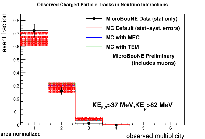
Figure 14: A bin-by-bin fitted, area normalized, CR background-subtracted, observed neutrino multiplicity distributions for MicroBooNE data overlaid with three GENIE predictions in linear scale. Data error bars include statistical errors obtained from the fit. Monte Carlo error bands include MC statistical errors from the fit and systematic error contributions added in quadrature.

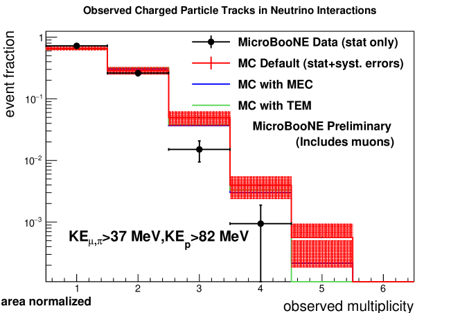
Figure 15: A bin-by-bin fitted, area normalized, CR background-subtracted, observed neutrino multiplicity distributions for MicroBooNE data overlaid with three GENIE predictions in log y scale. Data error bars include statistical errors obtained from the fit. Monte Carlo error bands include MC statistical errors from the fit and systematic error contributions added in quadrature.

6 Conclusion and Outlook

We have completed a preliminary analysis that compares the CR background-subtracted observed charged particle multiplicity distribution in a restricted final state phase space in MicroBooNE data to the predictions from three GENIE tunes processed through the MicroBooNE simulation and reconstruction.  Our analysis takes into account statistical uncertainties in a rigorous manner, and it estimates the impact of the largest expected systematic uncertainties.

We find all three GENIE tunes to be consistent within uncertainties with the data, although some weak evidence exists that GENIE under-predicts the number of one-prong events in the data and over-predicts multiplicities greater than two. The two alternative GENIE models considered here are not expected to yield significant multiplicity distribution differences; they were chosen to be used in this analysis simply because of their availability, and this analysis serves as proof of principle for future comparisons involving more widely varying model predictions in the future.

As part of this analysis we have developed a data-driven cosmic ray background estimation method based on the energy loss profile and multiple Coulomb scattering behavior of muons.  Within the available Monte Carlo statistics, we have shown that this method provides an unbiased estimate of the number of neutrino events in a pre-filtered sample, and given current statistical precision, it is independent of signal-to-background level and final state charged particle multiplicity.  This method could be applied to a broad range of charged current process measurements.

A future publication will use the full data set to reduce statistical uncertainties, compare to a wider range of neutrino event generator models, and present the data in a form that corrects for detector acceptance and efficiency and will be devoted to a measurement of charged particle multiplicity in MicroBooNE over a larger phase space.

References

- [1] “Design and Construction of the MicroBooNE Detector”, MicroBooNE Collaboration (R. Acciarri (Fermilab) et al), JINST 12 P022017 (2017).
- [2] “Neutrino flux prediction at MiniBooNE”, A. A. Aguilar-Arevalo et al. (MiniBooNE), Phys. Rev., D79, 072002 (2009).
- [3] J. A. Formaggio and G. P. Zeller, Rev. Mod. Phys. 84, 1307 (2013). See also contemporary discussions in Neutrino Cross Section Newsletter, T. Katori, ed., https://pprc.qmul.ac.uk/~katori/nu-xsec.html.
- [4] “Long-Baseline Neutrino Facility (LBNF) and Deep Underground Neutrino Experiment (DUNE) : Volume 2: The Physics Program for DUNE at LBNF”, DUNE Collaboration (R. Acciarri (Fermilab) et al.), e-Print: arXiv:1512.06148 [physics.ins-det] (2015).
- [5] “The GENIE Neutrino Monte Carlo Generator”, C. Andreopoulos, et al., Nucl.Instrum.Meth. A614 (2010) 87-104.
- [6] “GEANT4: A Simulation toolkit”, GEANT4 Collaboration (S. Agostinelli et al.), Nucl.Instrum.Meth. A506 (2003).
-
[7]
“Noise Characterization and Filtering in the
MicroBooNE TPC”, The MicroBooNE Collaboration,
https://www-microboone.fnal.gov/publications/publicnotes/MICROBOONE-NOTE-1016-PUB.pdf. -
[8]
“MicroBooNE Detector Stability”, The
MicroBooNE Collaboration,
https://www-microboone.fnal.gov/publications/publicnotes/MICROBOONE-NOTE-1013-PUB.pdf. - [9] “Larsoft: A software package for liquid argon time projection drift chambers”, E. D. Church, arXiv:1311.6774, 2016.
- [10] “Corsika: A monte carlo code to simulate extensive air showers”, Forschungszentrum Karlsruhe Report FZKA, 1998., https://www.ikp.kit.edu/corsika/70.php.
-
[11]
“Selection and kinematic properties of a
first charged-current numu inclusive event sample in MicroBooNE”, The
MicroBooNE Collaboration,
https://www-microboone.fnal.gov/publications/publicnotes/MICROBOONE-NOTE-1010-PUB.pdf. - [12] “The Review of Particle Physics (2016)”, C. Patrignani et al. (Particle Data Group), Chin. Phys. C, 40, 100001 (2016).
- [13] W.K. Sakumoto et.al, “Calibration of the CCFR Target Calorimeter”, Nucl.Instrum.Meth. A294 (1990) 179-192.
- [14] “The Pandora Software Development Kit for Pattern Recognition” J.S. Marshall and M.A. Thomson, Eur.Phys.J. C75 (2015).
-
[15]
“The Pandora multi-algorithm approach to
automated pattern recognition in LAr TPC detectors”, The MicroBooNE
Collaboration,
https://www-microboone.fnal.gov/publications/publicnotes/MICROBOONE-NOTE-1015-PUB.pdf. - [16] “The detection of back-to-back proton pairs in charged-current neutrino interactions with the ArgoNeuT detector in the NuMI low energy beam line”, ArgoNeuT Collaboration (R. Acciarri et al.), Phys. Rev. D 90, 012008 (2014)
-
[17]
“MINUIT: Function Minimization and Error Analysis”, F. James,
https://root.cern.ch/sites/d35c7d8c.web.cern.ch/files/minuit.pdf. -
[18]
“ROOT: Data Analysis Framework”,
https://root.cern.ch/.