A degenerate extension of the Schwarzschild exterior

Abstract

We present vacuum spacetime solutions of first order gravity, which are described by the exterior Schwarzschild geometry in one region and by degenerate tetrads in the other. The invertible and noninvertible phases of the tetrad meet at an intermediate boundary across which the components of the metric, affine connection and field-strength are all continuous. Within the degenerate spacetime region, the noninvertibility of the tetrad leads to nonvanishing torsion. In contrast to the Schwarzschild spacetime which is the unique spherically symmetric solution of Einsteinian gravity, all the field-strength components associated with these vacuum geometries remain finite everywhere.

I Introduction

In Einstein’s theory of gravity in vacuum, the Schwarzschild metric turns out to be the unique spherically symmetric solution. This geometry exhibits a curvature singularity at the origin. As long as the metric is demanded to be invertible and spherically symmetric, there seems to be no escape from such singular solutions in the classical theory. However, the first order gravity theory in vacuum admits, besides a phase with invertible tetrads (metric), another (non-Einsteinian) phase based on tetrads which have vanishing determinants and hence are not invertible. The classical theories for these two phases are not equivalent tseytlin . In fact, the solution space with noninvertible tetrads possesses a rich structure, as was elucidated in some recent studies kaul ; kaul1 . In view of this, it is worthwhile to explore whether there could be any extension of the Schwarzschild exterior geometry such that the full spacetime is regular everywhere, within a formulation of gravity theory that admits both the phases.

To deal with degenerate spacetime solutions in gravity theory, the appropriate starting point is the first order formulation based on Hilbert-Palatini action, which, unlike the second order formulation, does not require the explicit use of the inverse metric. This action functional is given in terms of two independent fields, the tetrad $e_{\mu}^{I}$ and the connection $\omega_{\mu}^{IJ}$, as:

$$S = \frac{1}{8\kappa^{2}}\int d^{4}x~{}\epsilon^{\mu\nu\alpha\beta}\epsilon_{IJKL}e_{\mu}^{I}e_{\nu}^{J}R_{\alpha\beta}^{~{}~{}KL}(\omega)$$ (1)

Here $R_{\mu\nu}^{~{}~{}IJ}(\omega)=\partial_{[\mu}\omega^{IJ}_{\nu]}+\omega^{IK}_{[\mu}\omega^{~{}~{}~{}J}_{\nu]K}$ is the field strength of the gauge connection $\omega_{\mu}^{IJ}$ corresponding to the local SO(3,1) Lorentz symmetry. The fields carry two kinds of indices: $\mu\equiv(t,a)\equiv(t,x,y,z)$ referring to the spacetime coordinates and $I\equiv(0,i)\equiv(0,1,2,3)$ to the local inertial (Lorentz) frame. Completely antisymmetric symbols $\epsilon^{\mu\nu\alpha\beta}$ and $\epsilon_{IJKL}$ take constant values $0$ and $\pm 1$ with $\epsilon^{txyz}=+1=\epsilon_{0123}$. The Euler-Lagrange equations of motion obtained by varying the action (1) independently with respect to $e_{\mu}^{I}$ and $\omega_{\mu}^{IJ}$ are:

$$\frac{\delta S}{\delta\omega_{\mu}^{IJ}}~{} : ~{}~{}~{}~{}\epsilon^{\mu\nu\alpha\beta}\epsilon_{IJKL}e_{\mu}^{K}D_{\nu}(\omega)e_{\alpha}^{L}=0$$ (2)

$$\frac{\delta S}{\delta e_{\mu}^{I}}~{} : ~{}~{}~{}~{}\epsilon^{\mu\nu\alpha\beta}\epsilon_{IJKL}e_{\nu}^{J}R_{\alpha\beta}^{~{}~{}KL}(\omega)=0$$ (3)

This set of equations admits both invertible and noninvertible tetrads as solutions. These reduce to Einstein’s equations in vacuum only in the invertible phase, where the vanishing of torsion emerges as a dynamical consequence. For noninvertible tetrads, however, the space of solutions consists of geometries that generically exhibit torsion even in vacuum tseytlin ; kaul ; kaul1 .

Here we attempt to construct a special class of spherically symmetric solutions of the equations of motion in pure gravity, which are characterized by the different phases of first order gravity in two different regions, one with non-degenerate tetrads and other with degenerate tetrads. In particular, we look for spacetime solutions with the exterior Schwarzschild metric in one region and a degenerate metric in the other. In addition, we demand that these must be associated with field-strength whose components do not diverge anywhere in the manifold and satisfy certain continuity properties at the boundary connecting the two regions.

Let us note that constructions similar in spirit to the ones discussed above have been attempted earlier bengtsson1 ; bengtsson ; madhavan . For example, Bengtsson bengtsson ; bengtsson1 has presented some spacetime solutions of the complex SU(2) formulation sen ; ashtekar of gravity theory with degenerate spatial (densitized) triads in the interior. In the explicit examples of real solutions that we shall exhibit here, the metrics, while being degenerate in a region, are associated with invertible triads.

In the next couple of sections, we present the construction of a class of vacuum solutions of first order gravity which exhibit the properties outlined above. There are a countably infinity of them, for each of which underlies a regular geometry everywhere. The concluding section contains a summary of the main results and a few observations regarding the possible importance of these newly found configurations in generic contexts.

II Region-I: Invertible tetrad

Let us first introduce a system of coordinates $(t,u,\theta,\phi)$ which cover the whole spacetime, with $\left(t\in(-\infty,\infty),~{}u\in(-\infty,\infty),~{}\theta\in[0,\pi],~{}\phi\in[0,2\pi]\right)$. In these coordinates, we define a spherically symmetric and static metric of the form bengtsson :

$$ds^{2}=-\left[1-\frac{2M}{f(u)}\right]dt^{2}+\left[1-\frac{2M}{f(u)}\right]^{-1}f^{\prime 2}(u)du^{2}+f^{2}(u)\left[d\theta^{2}+\sin^{2}\theta d\phi^{2}\right]$$ (4)

where, the monotonic function $f(u)$, which represents the radius of the two-sphere (at any fixed $t$ and $u$), satisfies the following properties:

$$f(u_{0})=2M,~{}~{}~{}~{}f^{\prime}(u_{0})=0~{}.$$ (5)

The metric (4) describes only a part of the full spacetime (region-I), corresponding to the values $u>u_{0}$ or $f(u)>2M$. The boundary $u=u_{0}$ represents a three-surface on which the metric determinant, $g=-f^{4}(u)f^{{}^{\prime}2}(u)\sin^{2}\theta$, vanishes. The constant parameter $M$ defines the area of the surface of the two sphere $S^{2}_{(\theta,\phi)}$ at $u=u_{0}$. For $f(u)>2M$, this metric is a vacuum solution of Einstein’s equations $R_{\mu\nu}=0$, which essentially corresponds to the phase with invertible metrics in first order gravity theory.

The tetrad fields in this region with $f(u)>2M$ can be read off from the metric (4) as:

$$e^{0}_{t}=\left(1-\frac{2M}{f(u)}\right)^{\frac{1}{2}},~{}e^{1}_{u}=\frac{f^{\prime}(u)}{\left(1-\frac{2M}{f(u)}\right)^{\frac{1}{2}}},~{}e_{\theta}^{2}=f(u),~{}e^{3}_{\phi}=f(u)\sin\theta$$ (6)

The nonvanishing components of the associated (torsionless) spin-connection fields $\omega_{\alpha}^{~{}IJ}$ are given by:

$$\omega^{01}=\frac{M}{f^{2}(u)}dt,~{}\omega^{12}=-\left(1-\frac{2M}{f(u)}\right)^{\frac{1}{2}}d\theta,~{}\omega^{23}=-\cos\theta d\phi,~{}\omega^{31}=\left(1-\frac{2M}{f(u)}\right)^{\frac{1}{2}}\sin\theta d\phi$$

Using these, the field strength tensors $R_{\mu\nu}^{~{}~{}IJ}(\omega)$ can be evaluated to be:

$$R^{01}(\omega) = \frac{2Mf^{\prime}(u)}{f^{3}(u)}dt\wedge du,~{}~{}~{}R^{02}(\omega)=-\frac{M}{f^{2}(u)}\left(1-\frac{2M}{f(u)}\right)^{\frac{1}{2}}dt\wedge d\theta,$$

$$~{}~{}R^{03}(\omega) = -\frac{M}{f^{2}(u)}\left(1-\frac{2M}{f(u)}\right)^{\frac{1}{2}}\sin\theta~{}dt\wedge d\phi,R^{12}(\omega)=-\frac{Mf^{\prime}(u)}{f^{2}(u)}\left(1-\frac{2M}{f(u)}\right)^{-\frac{1}{2}}du\wedge d\theta,$$

$$~{}R^{23}(\omega) = \frac{2M}{f(u)}\sin\theta~{}d\theta\wedge d\phi,~{}~{}~{}R^{31}(\omega)=-\frac{Mf^{\prime}(u)}{f^{2}(u)}\left(1-\frac{2M}{f(u)}\right)^{-\frac{1}{2}}\sin\theta~{}d\phi\wedge du$$ (8)

From the above set of fields, let us now construct their counterparts in the metric formulation, namely the affine connection $\Gamma_{\alpha\beta\rho}\equiv\Gamma_{\alpha\beta}^{~{}~{}\sigma}g_{\rho\sigma}$ and the spacetime field strength $R_{\mu\nu\rho\sigma}$, which are invariant under the internal $SO(3,1)$ rotations. Using the covariant constancy of the tetrad, given by the condition ${\cal D}_{\mu}e_{\nu}^{I}\equiv\partial_{\mu}e_{\nu}^{I}+\omega_{\mu}^{~{}IJ}e_{\nu J}-\Gamma_{\mu\nu}^{~{}~{}\rho}e_{\rho}^{I}=0$, the affine connection components are given in terms of the basic fields ($e_{\mu}^{I},~{}\omega_{\mu}^{~{}IJ})$ as:

$$\Gamma_{\mu\nu\rho}=e_{\rho I}\left[\partial_{\mu}e_{\nu}^{I}+\omega_{\mu}^{~{}IJ}e_{\nu J}\right]$$ (9)

Its nontrivial components are displayed below:

$$\Gamma_{ttu} = \frac{Mf^{\prime}(u)}{f^{2}(u)},~{}\Gamma_{tut}=-\frac{Mf^{\prime}(u)}{f^{2}}=\Gamma_{utt},~{}\Gamma_{uuu}=\frac{1}{2}\partial_{u}\left[\frac{f(u)f^{{}^{\prime}2}(u)}{f-2M}\right],$$

$$\Gamma_{\theta\theta u} = -f(u)f^{\prime}(u),~{}\Gamma_{u\theta\theta}=f(u)f^{\prime}(u)=\Gamma_{\theta u\theta},$$

$$\Gamma_{\phi\phi u} = -f(u)f^{\prime}(u)\sin^{2}\theta,~{}\Gamma_{u\phi\phi}=f(u)f^{\prime}(u)\sin^{2}\theta=\Gamma_{\phi u\phi},$$

$$\Gamma_{\phi\phi\theta} = -f^{2}(u)\sin\theta\cos\theta,~{}\Gamma_{\theta\phi\phi}=f^{2}(u)\sin\theta\cos\theta=\Gamma_{\phi\theta\phi}~{}.$$ (10)

The tensor $R_{\mu\nu\rho\sigma}$ is defined in terms of the $SO(3,1)$ field-strength as:

$$R_{\mu\nu\rho\sigma}=R_{\mu\nu}^{~{}IJ}(\omega)e_{\rho I}e_{\sigma J}~{},$$ (11)

whose nonvanishing components read:

$$R_{tutu}=-\frac{2Mf^{{}^{\prime}2}(u)}{f^{3}(u)},~{}R_{t\theta t\theta}=\frac{M[f(u)-2M]}{f^{2}(u)},~{}R_{t\phi t\phi}=\frac{M[f(u)-2M]}{f^{2}(u)}\sin^{2}\theta,$$

$$R_{u\theta u\theta}=-\frac{Mf^{{}^{\prime}2}(u)}{[f(u)-2M]},~{}R_{\theta\phi\theta\phi}=2Mf\sin^{2}\theta,~{}R_{\phi u\phi u}=-\frac{Mf^{{}^{\prime}2}(u)}{[f(u)-2M]}\sin^{2}\theta~{}.$$ (12)

In the region $u>u_{0}$ where tetrad is invertible and torsion is absent, the field strength tensor (11) reduces to the Riemann curvature tensor. However, this equality need not hold in general.

Choice of f(u) and boundary conditions:

Let us note that for $f(u)>2M$, the metric (4) is equivalent to the exterior Schwarzschild solution upto a coordinate transformation. This becomes evident upon the reparametrization $f(u)=r$, which brings this metric to the Schwarzschild form:

$$ds^{2}=-\left[1-\frac{2M}{r}\right]dt^{2}+\left[1-\frac{2M}{r}\right]^{-1}dr^{2}+r^{2}\left[d\theta^{2}+\sin^{2}\theta d\phi^{2}\right]$$ (13)

where $r$ is the radial coordinate. However, these two geometries are not equivalent at the degenerate surface $u=u_{0}$, where the coordinate transformation defined above becomes ill-defined.

Although $f(u)$ can be any monotonic function which obeys (i) the boundary conditions (5) and (ii) is such that it does not lead to divergences in any of the fields introduced above, it could nevertheless be more illuminating to work with a specific choice for $f(u)$. We choose:

$$f(u) = 2M\left[1+\left(\frac{u}{u_{0}}-1\right)^{n+1}\right]$$ (14)

where $n\geq 2$ is an integer. For these values of $n$, this function satisfies the above conditions (i) and (ii). At the degenerate boundary $u=u_{0}$, for the explicit choice (14), the nonvanishing components of the affine connection $\Gamma_{\mu\nu\rho}$ in (II) and $R_{\mu\nu\alpha\beta}$ tensor in (II) exhibit the following behaviour:

$$\Gamma_{\phi\phi\theta}=-\Gamma_{\theta\phi\phi}=-\Gamma_{\phi\theta\phi}\doteq-4M^{2}\sin\theta\cos\theta~{};$$

$$R_{\theta\phi\theta\phi}\doteq 4M^{2}\sin^{2}\theta~{}.$$ (15)

where the symbol $\doteq$ denotes equality only at $u=u_{0}$.

The set of fields constructed above defines the vacuum spacetime in the region-I, $u>u_{0}$ ($f(u)>2M$), completely. The analysis for the other region $u\leq u_{0}$ is presented next.

III Region-II: Noninvertible tetrad

As emphasized already, our purpose here is to construct degenerate spacetime solutions of the first order equations of motion (2) and (3) in the region $u\leq u_{0}$ (region-II). To begin with, we consider a degenerate metric with $g_{tt}=0$ everywhere in this region:

$$\hat{ds}^{2}_{(4)}=0+\sigma F^{2}(u)du^{2}+H^{2}(u)\left[d\theta^{2}+\sin^{2}\theta d\phi^{2}\right]$$ (16)

The nondegenerate 3-subspace of this metric exhibits the topology $S^{2}\times R$, which is the same as that of any $t=const.$ slice of the metric (4) in region-I. The two possible values of $\sigma=\pm 1$ correspond to an Euclidean or a Lorentzian 3-subspace, respectively. For $\sigma=+1$, $u$ is a spacelike coordinate whereas for $\sigma=-1$, it is timelike (in region-II). The continuity of the metric requires that the two arbitrary functions $F(u)$ and $H(u)$, whose precise forms are to be determined using the equations of motion, should have the following behaviour at the degenerate boundary:

$$F(u_{0})=0,~{}~{}~{}~{}H(u_{0})=2M~{}.$$ (17)

The internal (Lorentzian) metric is given by: $\eta_{IJ}=diag[-\sigma,\sigma,1,1]$. The tetrad fields are:

$$\hat{e}^{I}_{\mu}~{}=~{}\left(\begin{array}[]{cccc}0&0&0&0\\ 0&F(u)&0&0\\ 0&0&H(u)&0\\ 0&0&0&H(u)\sin\theta\end{array}\right)~{}=~{}\left(\begin{array}[]{cc}0&0\\ 0&\hat{e}_{a}^{i}\end{array}\right)$$ (24)

The only non-vanishing components of the torsionless spin-connection fields $\bar{\omega}_{a}^{~{}ij}(\hat{e})={\frac{1}{2}}\left[\hat{e}^{b}_{i}\partial_{[a}\hat{e}_{b]}^{j}-\hat{e}^{b}_{j}\partial_{[a}\hat{e}_{b]}^{i}-\hat{e}_{a}^{l}\hat{e}^{b}_{i}\hat{e}^{c}_{j}\partial_{[b}\hat{e}_{c]}^{l}\right]$, which are determined completely by the triads $\hat{e}_{a}^{i}$, are given by:

$$\bar{\omega}_{\theta}^{12}=-\sigma\frac{H^{\prime}(u)}{F(u)},~{}\bar{\omega}_{\phi}^{23}=-\cos\theta,~{}\bar{\omega}_{\phi}^{31}=\sigma\frac{H^{\prime}(u)}{F(u)}\sin\theta$$ (25)

The corresponding $SO(3,1)$ field strength components read:

$$\bar{R}_{u\theta}^{~{}12}(\bar{\omega})=-\sigma\left[\frac{H^{\prime}(u)}{F(u)}\right]^{\prime},~{}\bar{R}_{\theta\phi}^{~{}23}(\bar{\omega})=\left[1-\sigma\left(\frac{H^{\prime}(u)}{F(u)}\right)^{2}\right]\sin\theta,~{}\bar{R}_{\phi u}^{~{}31}(\bar{\omega})=-\sigma\left[\frac{H^{\prime}(u)}{F(u)}\right]^{\prime}\sin\theta$$

(26)

Given the tetrad fields (24) above, we now look for the most general set of connection fields $\hat{\omega}_{\mu}^{IJ}\equiv(\hat{\omega}_{t}^{0i},~{}\hat{\omega}_{t}^{ij},~{}\hat{\omega}_{a}^{ij},~{}\hat{\omega}_{a}^{0i})$ which solve the equations of motion (2). Using the fact that the components $\hat{\omega}_{a}^{ij}$ can be written as a sum of the connection $\bar{\omega}_{a}^{ij}(\hat{e})$ without torsion and the contortion $K_{a}^{ij}$:

$$\hat{\omega}_{a}^{ij}=\bar{\omega}_{a}^{ij}(\hat{e})+K_{a}^{ij}~{},$$ (27)

the most general solution of the equations of motion (2) is then given by kaul :

$$K_{a}^{ij}=\epsilon^{ijk}\hat{e}_{a}^{l}N_{kl},~{}\hat{\omega}_{a}^{0i}=\hat{e}_{al}M^{il},~{}\hat{\omega}_{t}^{0i}=0=\hat{\omega}_{t}^{ij}~{},$$ (28)

where the spacetime-dependent matrices $N_{kl}=N_{lk}$ and $M_{kl}=M_{lk}$ are symmetric but arbitrary otherwise. The existence of these arbitrary fields is essentially a reflection of the fact that in first order gravity theory with noninvertible tetrads, the equations of motion leave some of the connection components completely undetermined. In what follows next, we will restrict our attention to the simpler case with $M_{kl}=0$. The remaining set of six fields $N_{kl}$ can be represented as:

$$N_{ij}~{}=~{}\left(\begin{array}[]{ccc}\alpha&\eta_{3}&\eta_{2}\\ \eta_{3}&\beta&\eta_{1}\\ \eta_{2}&\eta_{1}&\gamma\end{array}\right)$$ (32)

Using this parametrization of $N_{ij}$ and the triads (24), the components of the contortion $K_{a}^{ij}$ as in (28) become:

$$K^{12} = \eta_{2}F(u)du+H(u)\left[\eta_{1}d\theta+\gamma\sin\theta d\phi\right]$$

$$K^{23} = \alpha F(u)du+H(u)\left[\eta_{3}d\theta+\eta_{2}\sin\theta d\phi\right]$$

$$K^{31} = \eta_{3}F(u)du+H(u)\left[\beta d\theta+\eta_{1}\sin\theta d\phi\right]$$ (33)

With these, the full connection coefficients $\hat{\omega}^{IJ}$ are given by:

$$\hat{\omega}^{01} = \hat{\omega}^{02}=\hat{\omega}^{03}=0~{},$$

$$\hat{\omega}^{12} = \eta_{2}F(u)du+\left[\eta_{1}H(u)-\sigma\frac{H^{\prime}(u)}{F(u)}\right]d\theta+\gamma H(u)\sin\theta d\phi~{},$$

$$\hat{\omega}^{23} = \alpha F(u)du+\eta_{3}H(u)d\theta+\left[\eta_{2}H(u)\sin\theta-\cos\theta\right]d\phi~{},$$

$$\hat{\omega}^{31} = \eta_{3}F(u)du+\beta H(u)d\theta+\left[\eta_{1}H(u)+\sigma\frac{H^{\prime}(u)}{F(u)}\right]\sin\theta d\phi~{}.$$ (34)

For these connection fields, the field-strength can be evaluated to be:

$$\hat{R}^{01}(\hat{\omega}) = \hat{R}^{02}(\hat{\omega})=\hat{R}^{03}(\hat{\omega})=0~{},$$

$$\hat{R}^{12}(\hat{\omega}) = Fd\eta_{2}\wedge du+d\left(\eta_{1}H\right)\wedge d\theta+\sin\theta d(\gamma H)\wedge d\phi+\left[(\eta_{3}^{2}-\alpha\beta)HF-\sigma\left(\frac{H^{\prime}}{F}\right)^{\prime}\right]du\wedge d\theta$$

$$+ \left[\gamma H\cos\theta-\eta_{3}H\left(\eta_{1}H+\sigma\frac{H^{\prime}}{F}\right)\sin\theta+\beta H(\eta_{2}H\sin\theta-\cos\theta)\right]d\theta\wedge d\phi$$

$$+ \left[\alpha F\left(\eta_{1}H+\sigma\frac{H^{\prime}}{F}\right)\sin\theta-\eta_{3}F(\eta_{2}H\sin\theta-\cos\theta)\right]d\phi\wedge du~{},$$

$$\hat{R}^{23}(\hat{\omega}) = Fd\alpha\wedge du+d(\eta_{3}H)\wedge d\theta+\sin\theta d(\eta_{2}H)\wedge d\phi+\left[\eta_{3}H^{\prime}+\sigma(\eta_{2}\beta-\eta_{1}\eta_{3})FH\right]du\wedge d\theta$$

$$+ \left[\eta_{2}H\cos\theta+\sin\theta-\sigma\gamma\beta H^{2}\sin\theta+\sigma\left(\eta_{1}H-\frac{H^{\prime}}{F}\right)\left(\eta_{1}H+\frac{H^{\prime}}{F}\right)\sin\theta\right]d\theta\wedge d\phi$$

$$+ \left[-\eta_{2}H^{\prime}+\sigma(\eta_{3}\gamma-\eta_{1}\eta_{2})FH\right]\sin\theta d\phi\wedge du~{},$$

$$\hat{R}^{31}(\hat{\omega}) = Fd\eta_{3}\wedge du+d(\beta H)\wedge d\theta+\sin\theta d(\eta_{1}H)\wedge d\phi+\left[-\sigma\alpha H^{\prime}+(\alpha\eta_{1}-\eta_{2}\eta_{3})FH\right]du\wedge d\theta$$ (35)

$$+ \left[\gamma\eta_{3}H^{2}\sin\theta+\left(\eta_{1}H+\sigma\frac{H^{\prime}}{F}\right)\cos\theta-\left(\eta_{1}H-\sigma\frac{H^{\prime}}{F}\right)\left(\eta_{2}H\sin\theta-\mathrm{cos}\theta\right)\right]d\theta\wedge d\phi$$

$$+ \left[\left((\eta_{2}^{2}-\alpha\gamma)FH-\sigma\left(\frac{H^{\prime}}{F}\right)^{\prime}\right)\sin\theta-\eta_{2}F\cos\theta\right]d\phi\wedge du~{}.$$

This in turn leads to the following identity:

$$\hat{e}_{u}^{1}\hat{R}_{\theta\phi}^{~{}23}(\hat{\omega})+\hat{e}_{\theta}^{2}\hat{R}_{\phi u}^{~{}31}(\hat{\omega})+\hat{e}_{\phi}^{3}\hat{R}_{u\theta}^{~{}12}(\hat{\omega}) = \left[(\sigma\eta_{1}^{2}+\eta_{2}^{2}+\eta_{3}^{2}-\alpha\beta-\sigma\beta\gamma-\gamma\alpha)FH^{2}\right]\sin\theta$$ (36)

$$+ \left[\left(1-\sigma\frac{H^{\prime 2}}{F^{2}}\right)F-2\sigma H\left(\frac{H^{\prime}}{F}\right)^{\prime}\right]\sin\theta$$

Following kaul , it is straight forward to check that the configuration described above satisfy the remaining set of equations of motion (3) provided the contortion fields are constrained as:

$$\left(\sigma\eta_{1}^{2}+\eta_{2}^{2}+\eta_{3}^{2}-\alpha\beta-\sigma\beta\gamma-\gamma\alpha\right)FH^{2}+\left(1-\sigma\frac{H^{\prime 2}}{F^{2}}\right)F-2\sigma H\left(\frac{H^{\prime}}{F}\right)^{\prime}=0$$ (37)

Hence, the set of degenerate tetrad (24) and the connection fields (III), subject to the above constraint, solves both the equations of motion (2) and (3) of first order gravity theory in vacuum. These define the geometry of region II.

IV Joining regions I and II: Full spacetime Solution(s)

Let us now construct a complete solution for $-\infty<u<\infty$ by finding the explicit functional forms of the torsional fields as well as of $F(u)$ and $H(u)$, such that the constraint (37) is obeyed and all the components of the metric, affine connection and the field strength are continuous across the $u=u_{0}$ hypersurface which connects regions I and II. Just for the sake of simplicity, in the rest of our analysis we choose a simpler setting where only one of the six torsional fields is nonvanishing and depends only on $u$:

$$\eta_{1}=\eta(u),~{}\eta_{2}=0,~{}\eta_{3}=0,~{}\alpha=0,~{}\beta=0,~{}\gamma=0.$$ (38)

For this choice, the nonvanishing components of the affine connection $\hat{\Gamma}_{\mu\nu\rho}=\hat{e}_{\rho I}\left[\partial_{\mu}\hat{e}_{\nu}^{I}+\hat{\omega}_{\mu}^{~{}IJ}\hat{e}_{\nu J}\right]$ (which contain torsion now) are evaluated to be:

$$\hat{\Gamma}_{uuu} = \sigma F(u)F^{\prime}(u),~{}\hat{\Gamma}_{\theta\theta u}=\sigma H(u)F(u)\left(\eta(u)H(u)-\sigma\frac{H^{\prime}(u)}{F(u)}\right)=-\hat{\Gamma}_{\theta u\theta},~{}\hat{\Gamma}_{u\theta\theta}=H(u)H^{\prime}(u),$$

$$\hat{\Gamma}_{\phi\phi u} = -\sigma H(u)F(u)\left(\eta(u)H(u)+\sigma\frac{H^{\prime}(u)}{F(u)}\right)\sin^{2}\theta=-\hat{\Gamma}_{\phi u\phi},~{}\hat{\Gamma}_{u\phi\phi}=H(u)H^{\prime}(u)\sin^{2}\theta,$$

$$\hat{\Gamma}_{\phi\phi\theta} = -H^{2}(u)\sin\theta\cos\theta=-\hat{\Gamma}_{\phi\theta\phi}=-\hat{\Gamma}_{\theta\phi\phi}~{}.$$ (39)

The spacetime field strength $\hat{R}_{\mu\nu\alpha\beta}=\hat{R}_{\alpha\beta}^{~{}IJ}(\hat{\omega})\hat{e}_{\mu I}\hat{e}_{\nu J}$ in this case becomes:

$$\hat{R}_{u\theta u\theta} = \sigma\left(\eta(u)H(u)-\sigma\frac{H^{\prime}(u)}{F(u)}\right)^{\prime}F(u)H(u)~{},$$

$$\hat{R}_{\theta\phi\theta\phi} = \left[1+\sigma\left(\eta(u)H(u)-\frac{H^{\prime}(u)}{F(u)}\right)\left(\eta(u)H(u)+\frac{H^{\prime}(u)}{F(u)}\right)\right]H^{2}(u)\sin^{2}\theta~{},$$

$$\hat{R}_{\phi u\phi u} = -\sigma\left(\eta(u)H(u)+\sigma\frac{H^{\prime}(u)}{F(u)}\right)^{\prime}F(u)H(u)\sin^{2}\theta$$ (40)

while all the other components turn out to be zero. In particular, the components $\hat{R}_{tutu},~{}\hat{R}_{t\theta t\theta}$ and $\hat{R}_{t\phi t\phi}$ vanish everywhere in the region-II ($u\leq u_{0}$). This is to be contrasted with the behaviour in region-I where the field strength components $R_{tutu},~{}R_{t\theta t\theta}$ and $R_{t\phi t\phi}$ as presented in (II) are zero only at the boundary.

For the choice (38), the constraint (37) among the fields $\eta(u),H(u),F(u)$ reduces to:

$$\eta^{2}FH^{2}+\left(\sigma-\frac{H^{\prime 2}}{F^{2}}\right)F-2H\left(\frac{H^{\prime}}{F}\right)^{\prime}=0$$ (41)

This provides only one condition among the three unknown fields. Since there are no more equations of motion that could be used to solve for these, we have the freedom of choosing two further constraints, such that the continuity properties at $u=u_{0}$ are satisfied. To this end, let us consider the following ansatze:

$$\eta(u) = \sigma\frac{H^{\prime}(u)}{F(u)H(u)},$$

$$\frac{H^{\prime}(u)}{F(u)} = \beta e^{\alpha(u-u_{0})}(u_{0}-u)^{m}$$ (42)

where $\alpha>0$ and $\beta$ are real-valued constants and $m$ can be an integer or a half-integer. With this, the components in eq.(IV) simplify to:

$$\hat{R}_{u\theta u\theta}=0,~{}\hat{R}_{\theta\phi\theta\phi}=H^{2}(u)\sin^{2}\theta,~{}\hat{R}_{\phi u\phi u}=-2\left(\frac{H^{\prime}(u)}{F(u)}\right)^{\prime}F(u)H(u)\sin^{2}\theta~{}.$$ (43)

The three equations in (41) and (IV) now can be solved for the three fields $H(u),F(u)$ and $\eta(u)$, leading to:

$$F(u) = 4\sigma\beta M\left[\alpha(u_{0}-u)^{m}-m(u_{0}-u)^{m-1}\right]~{}e^{\left[\alpha(u-u_{0})+\sigma\beta^{2}(u_{0}-u)^{2m}e^{2\alpha(u-u_{0})}\right]},$$

$$H(u) = 2M~{}e^{\left[\sigma\beta^{2}(u_{0}-u)^{2m}e^{2\alpha(u-u_{0})}\right]},$$

$$\eta(u) = \sigma\frac{\beta}{2M}(u_{0}-u)^{m}e^{\left[\alpha(u-u_{0})-\sigma\beta^{2}(u_{0}-u)^{2m}e^{2\alpha(u-u_{0})}\right]}$$ (44)

The constant $\alpha$ can be fixed by using the freedom in choosing the origin of $u$ coordinate. If we choose $u=0$ to be the point where the radius of the two sphere ($H(u)$) is extremum, then we have $\alpha=\frac{m}{u_{0}}$ for a fixed $m$. The requirement of continuity of the metric components $g_{\mu\nu}$ at $u=u_{0}$ fixes the other constant $\beta$ along with the number $m$ as:

$$\beta=u_{0}^{-m},~{}~{}~{}~{}~{}m=\frac{n+1}{2}$$

where $n\geq 2$ is the same integer appearing in the definition of $f(u)$ in eq.(14). This leads to two sets of solutions. The first one, corresponding to $\sigma=+1$, are represented by the following fields:

$$F(u) = -\frac{4M}{u_{0}^{2}}pu\left(1-\frac{u}{u_{0}}\right)^{p-1}e^{\left[p\left(\frac{u}{u_{0}}-1\right)+\left(\frac{u}{u_{0}}-1\right)^{2p}e^{2p\left(\frac{u}{u_{0}}-1\right)}\right]},$$

$$H(u) = 2M~{}e^{\left[\left(\frac{u}{u_{0}}-1\right)^{2p}e^{2p\left(\frac{u}{u_{0}}-1\right)}\right]},$$

$$\eta(u) = \frac{1}{2M}\left(1-\frac{u}{u_{0}}\right)^{p}e^{\left[p\left(\frac{u}{u_{0}}-1\right)-\left(\frac{u}{u_{0}}-1\right)^{2p}e^{2p\left(\frac{u}{u_{0}}-1\right)}\right]}~{},$$ (45)

where $p=\frac{n+1}{2}\geq 2$ is an integer. The other set with $\sigma=-1$ is given by:

$$F(u) = \frac{4M}{u_{0}^{2}}lu\left(1-\frac{u}{u_{0}}\right)^{l-1}e^{\left[l\left(\frac{u}{u_{0}}-1\right)+\left(\frac{u}{u_{0}}-1\right)^{2l}e^{2l\left(\frac{u}{u_{0}}-1\right)}\right]},$$

$$H(u) = 2M~{}e^{\left[\left(\frac{u}{u_{0}}-1\right)^{2l}e^{2l\left(\frac{u}{u_{0}}-1\right)}\right]},$$

$$\eta(u) = -\frac{1}{2M}\left(1-\frac{u}{u_{0}}\right)^{l}e^{\left[l\left(\frac{u}{u_{0}}-1\right)-\left(\frac{u}{u_{0}}-1\right)^{2l}e^{2l\left(\frac{u}{u_{0}}-1\right)}\right]}~{},$$ (46)

where $l=\frac{n+1}{2}\geq\frac{3}{2}$ is a half-integer. With this, we have a countable infinity of vacuum solutions of the first order equations of motion, parametrized by the integer $n\geq 2$, whose odd or even values correspond to $\sigma=+1$ and $\sigma=-1$, respectively. The metric components $g_{\mu\nu}(u)$ are $C^{n}$ functions. Note that the parameter $M$ has the interpretation of being the inverse of the contortion $\eta$ at the extremal point $u=0$ upto a numerical constant that depends on $n$.

For the solutions displayed above, the nonvanishing components of the affine connection and the field strength at the boundary $u=u_{0}$ are given by:

$$\hat{\Gamma}_{\phi\phi\theta} = -\hat{\Gamma}_{\phi\theta\phi}=-\hat{\Gamma}_{\theta\phi\phi}\doteq-4M^{2}\sin\theta\cos\theta~{};$$

$$\hat{R}_{\theta\phi\theta\phi} \doteq 4M^{2}\sin^{2}\theta~{}.$$ (47)

Comparing of these with the corresponding boundary values (II) for the nondegenerate region, we note that the set of $SO(3,1)$ invariant fields are all continuous at $u=u_{0}$:

$$g_{\rho\sigma}\doteq\hat{g}_{\rho\sigma},~{}\Gamma_{\rho\sigma\alpha}\doteq\hat{\Gamma}_{\rho\sigma\alpha},~{}R_{\alpha\beta\rho\sigma}\doteq\hat{R}_{\alpha\beta\rho\sigma}~{}.$$ (48)

Of the original $SO(3,1)$ valued fields, while all the tetrad and field strength components are continuous across the separating degenerate boundary, some connection components, which are pure gauge on the boundary, are not continuous. But all the $SO(3,1)$ invariant fields as reflected in (48) are continuous across this boundary.

Let us look at the nature of geometries in the region-II as represented by the fields given in eqs.(IV) and (IV) in detail. For both these sets, the fields have the following boundary behaviour:

$$F(u)\rightarrow 0,~{}H(u)\rightarrow 2M,~{}\eta(u)\rightarrow 0~{}\mathrm{~{}~{}as}~{}u\rightarrow-\infty~{}\mathrm{or~{}}u\rightarrow u_{0}.$$ (49)

Note that the radius $H(u)$ of the two-sphere is finite and nonvanishing everywhere. For $\sigma=+1$, it has a maximum value at $u=0$, given by $H_{max}=2M\exp(e^{-2p})>2M$ (for a fixed integer $p\geq 2$). On the other hand, for $\sigma=-1$, it exhibits a minimum value at $u=0$, with $H_{min}=2M\exp(-e^{-2l})<2M$ (for a fixed half-integer $l\geq\frac{3}{2}$). This has been displayed in the Fig.1 where the profile of the radius of two-sphere $R(u)=f(u)$ for the region-I ($u>u_{0}$) and $R(u)=H(u)$ for the region-II ($u\leq u_{0}$) has been presented. The interpretation of the two free parameters $M$ and $u_{0}$ in each solution is now apparent: they characterize the area and location of the hypersurface at $u=u_{0}$, respectively.

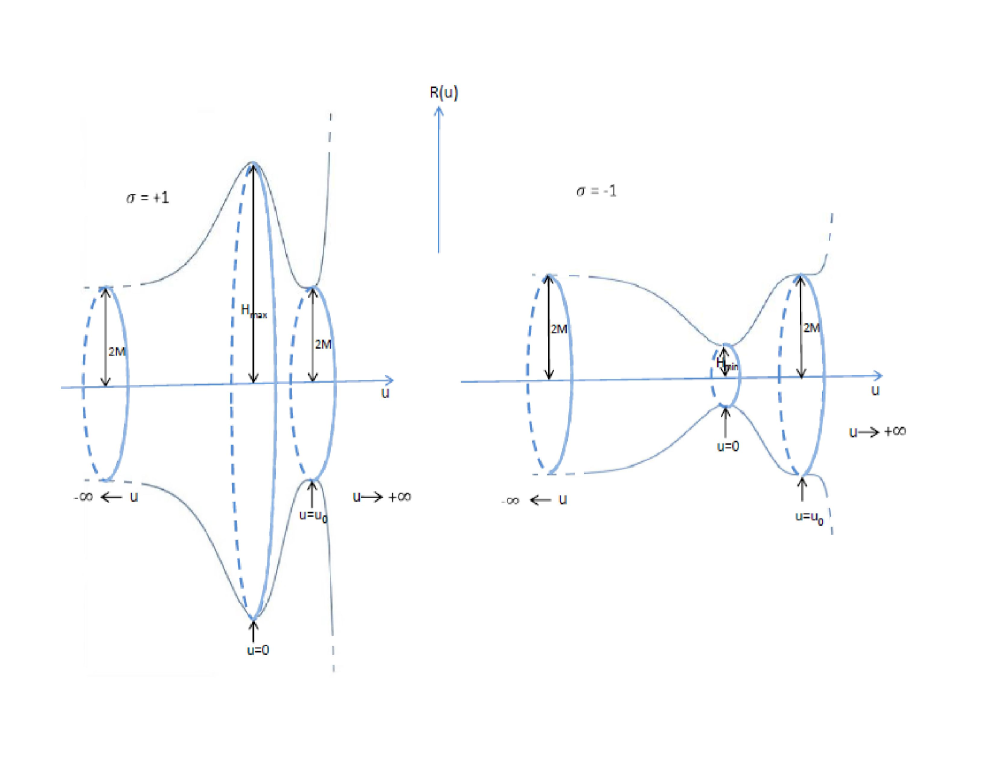
Figure 1: Pictorial representation of spacetime solutions for $\sigma=\pm 1$ at any fixed $t$

The behaviour of the contortion field $\eta(u)$, which is localized entirely within region-II around the origin $u=0$, has been been provided in Fig.2. The profiles for $\sigma=\pm 1$ are qualitatively the same (for any fixed integer $p\geq 2$ or any fixed half integer $l\geq\frac{3}{2}$), the extrema being at $u=0$.

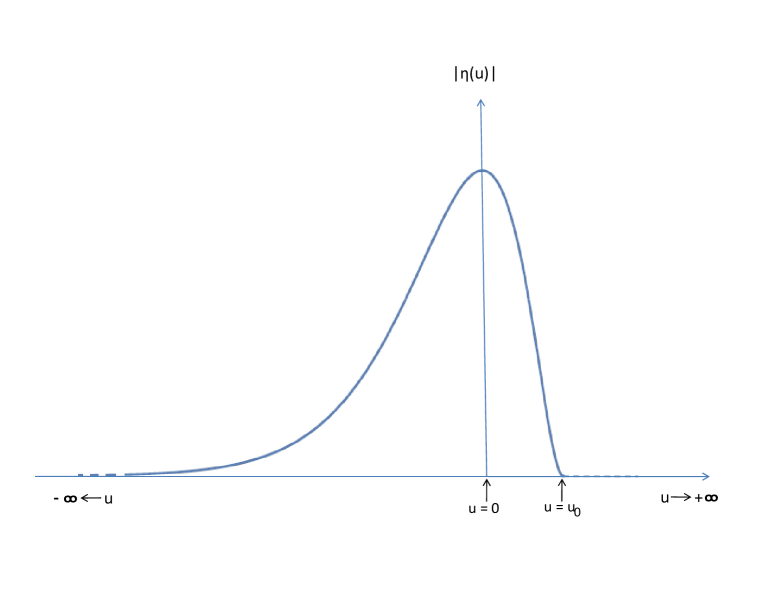
Figure 2: Contortion field $\eta(u)$ for $\sigma=\pm 1$

It should be emphasized that the spacetime field strength components $\hat{R}_{\mu\nu\rho\sigma}$ are finite everywhere in the range $-\infty<u<\infty$. Although it is not possible to construct scalars from the fields $\hat{R}_{\mu\nu\rho\sigma}$ (unless they are topological) associated with a noninvertible 4-metric, one can nevertheless look at the scalars associated with the nondegenerate 3-subspace described by $(e_{a}^{i},~{}\hat{\omega}_{b}^{kl})$. These are well-behaved in the entire domain:

$$\hat{R}(\hat{\omega})=\hat{e}^{a}_{i}\hat{e}^{b}_{j}\hat{R}_{ab}^{~{}ij}(\hat{\omega})=0;$$

$$\hat{R}_{ab}^{~{}ij}(\hat{\omega})\hat{R}^{ab}_{~{}ij}(\hat{\omega})=\hat{R}_{u\theta}^{~{}12}(\hat{\omega})\hat{R}^{u\theta}_{~{}12}(\hat{\omega})+\hat{R}_{\theta\phi}^{~{}23}(\hat{\omega})\hat{R}^{\theta\phi}_{~{}23}(\hat{\omega})+\hat{R}_{\phi u}^{~{}31}(\hat{\omega})\hat{R}^{\phi u}_{~{}31}(\hat{\omega})=\frac{4}{H^{4}(u)}$$

The configurations described above are to be contrasted with the Schwarzschild spacetime, which is the unique spherically symmetric solution of Einsteinian gravity and is associated with divergent field strength components $R_{trtr},~{}R_{t\theta t\theta}$ and $R_{t\phi t\phi}$ at the origin.

V conclusions

First order formulation of classical gravity theory in four dimensions admits degenerate spacetimes as vacuum solutions. Based on this observation, we have constructed a class of spherically symmetric geometries with two regions which are associated with invertible and noninvertible tetrads. As the field configurations in both these regions satisfy the first order equations of motion in pure gravity and are continuous across the degenerate boundary connecting them, the full spacetime as a whole represents a vacuum solution of gravity theory. In the region with non-degenerate metric, away from the separating boundary, the spacetime geometry is equivalent to that of the Schwarzschild exterior.

The most remarkable property of these solutions are reflected through the field-strength components, which are well-behaved everywhere. In this sense these spacetimes are regular, since any curvature singularity is typically a reflection of the divergence in the individual field strength components. It should be emphasized that the existence of these solutions of the first order equations of motion is not in any way in conflict with Birkhoff’s theorem, which concerns solely the invertible phase ($\det g_{\mu\nu}\neq 0$) of pure gravity.

Within the degenerate region, as described by the associated noninvertible metric, the spacetime essentially becomes two-dimensional at the points $u=u_{0}$, $u=0$ and also at $u\rightarrow-\infty$ which is one of the asymptotic boundaries. It is not clear at this stage whether such a phenomenon really does encode a change of spacetime topology in classical gravity.

The general framework presented here can also be used to construct vacuum solutions in first order gravity theory with multiple regions containing degenerate and non-degenerate geometries. In particular, one such solution with two regions of flat spacetime separated by a finite sized bridge which has a non-invertible metric has been presented in ref sandipan .

Finally, let us note that the configurations discussed here correspond to finite (vanishing) action. Fluctuations around these saddle points might encode nontrivial contributions to the path integral of quantum gravity. These vacuum geometries may be expected to be relevant in other formulations of quantum gravity as well.

References

(1) A.A. Tseytlin, J. Phys. A: Math. Gen. 15
(1982) L105.
(2) R.K. Kaul and S. Sengupta, Phys. Rev. D 93,
084026 (2016)
(3) R.K. Kaul and S. Sengupta, Phys. Rev. D 94,
104047 (2016)
(4) I. Bengtsson, Gen. Relat. Gravit. 25 (1993)
101–112.
(5) I. Bengtsson, Class. Quantum Grav. 8 (1991)
1847-1858.
(6) M. Varadarajan, Class. Quantum Grav. 8 (1991)
11, L235-L240.
(7) A. Sen, Phys. Lett. B 119 (1982) 89-91.
(8) A. Ashtekar, Phys. Rev. Lett. 57 (1986)
2244-2247;
A. Ashtekar, Phys. Rev. D36 (1987) 1587-1602.
(9) S. Sengupta, Spacetime-bridge solutions in
vacuum gravity, arXiv:1708.04971 [gr-qc] (2017)