Breaks in surface brightness profiles and radial abundance gradients in the discs of spiral galaxies

We examine the relation between breaks in the surface brightness profiles and radial abundance gradients within the optical radius in the discs of 134 spiral galaxies from the CALIFA survey. The distribution of the radial abundance (in logarithmic scale) in each galaxy was fitted by simple and broken linear relations. The surface brightness profile was fitted assuming pure and broken exponents for the disc. We find that the maximum absolute difference between the abundances in a disc given by broken and pure linear relations is less than 0.05 dex in the majority of our galaxies and exceeds the scatter in abundances for 26 out of 134 galaxies considered. The scatter in abundances around the broken linear relation is close (within a few percent) to that around the pure linear relation. The breaks in the surface brightness profiles are more prominent. The scatter around the broken exponent in a number of galaxies is lower by a factor of two or more than that around the pure exponent. The shapes of the abundance gradients and surface brightness profiles within the optical radius in a galaxy may be different. A pure exponential surface brightness profile may be accompanied by a broken abundance gradient and vise versa. There is no correlation between the break radii of the abundance gradients and surface brightness profiles. Thus, a break in the surface brightness profile does not need to be accompanied by a break in the abundance gradient.

1 Introduction

It was established many years ago (de Vaucouleurs 1959; Freeman 1970; van der Kruit 1979) that the surface brightness profiles of the discs of spiral galaxies can be fitted by an exponential. However, pure exponential functions can give only a rough representation of the radial surface brightness profiles of the discs of some galaxies. Pohlen & Trujillo (2006) found that only around 10 to 15 per cent of all spiral galaxies have a normal/standard purely exponential disc, while the surface brightness distribution of the rest of the galaxies is better described by a broken exponential.

It is also well-known that discs of spiral galaxies show negative radial abundance gradients in the sense that the abundance is higher at the centre and decreases with galactocentric distance (Searle 1971; Smith 1975). It is common practice to express the oxygen abundance in a galaxy using the logarithmic scale, which permits one to describe the abundance distribution across the disc of a galaxy with a linear relation between oxygen abundance O/H and galactocentric distance $R{{}_{g}}$ ; we used fractional galactocentric distances $R{{}_{g}}$ normalized to the optical isophotal radius $R_{25}$ in the current study.

The variation in the (logarithm of) abundance with radius has been examined for many galaxies by different authors (Vila-Costas & Edmunds 1992; Zaritsky et al. 1994; Ryder 1995; van Zee et al. 1998; Pilyugin et al. 2004, 2006, 2007, 2014a, 2015; Moustakas et al. 2010; Gusev et al. 2012; Sánchez et al. 2014; Zinchenko et al. 2015; Ho et al. 2015; Bresolin & Kennicutt 2015, among many others). Previous studies found that the gradients are reasonably well fitted by a straight line although in some spiral galaxies the slope appears to steepen (or flatten) in the central regions (Vila-Costas & Edmunds 1992; Zaritsky 1992; Martin & Roy 1995; Zahid & Bresolin 2011; Scarano et al. 2011; Sánchez et al. 2014; Zinchenko et al. 2016, among many others). For example, the abundance gradient in the disc of the Milky Way traced by Cepheid abundances seems to flatten in the central region (Martin et al. 2015; Andrievsky et al. 2016).

There is a correlation between the local oxygen abundance and stellar surface brightness in the discs of spiral galaxies (e.g. Webster & Smith 1983; Edmunds & Pagel 1984; Ryder 1995; Moran et al. 2012; Rosales-Ortega et al. 2012; Pilyugin et al. 2014b). If this relation is indeed local, i.e. if there is a point-to-point relation between the surface brightness and abundance, then one can expect that the break in the surface brightness distribution should be accompanied by a break in the abundance distribution.

The existence of breaks in gradients reported in earlier works can be questioned for two reasons. Firstly, those gradients are typically based on a small number of H ii region abundances. Secondly, it has been recognized that the shape of the abundance distribution is very sensitive to the calibration used for the abundance determinations (e.g. Zaritsky et al. 1994; Kennicutt & Garnett 1996; Pilyugin 2001, 2003). Zaritsky et al. (1994) pointed out that the question of the shape of the abundance gradient remains open and can be solved only when measurements of many H ii region abundances per galaxy and a reliable method for abundance determinations become available.

Recently, measurements of spectra of dozens of H ii regions in several galaxies were obtained (e.g. Berg et al. 2015; Croxall et al. 2015, 2016). In the framework of surveys such as the Calar Alto Legacy Integral Field Area (CALIFA) survey (Sánchez et al. 2012; Husemann et al. 2013; García-Benito et al. 2015) and the Mapping Nearby Galaxies at Apache Point Observatory (MaNGA) survey (Bundy et al. 2015), 2D spectroscopy of a large number of galaxies is being carried out. This 2D spectroscopy provides the possibility to determine elemental abundances across these objects and to construct abundance maps for the targeted galaxies. This permits one to investigate the abundance distribution across the disc in detail. In particular, the radial oxygen abundance distributions in the discs of galaxies can be examined (Sánchez et al. 2014; Zinchenko et al. 2016).

A new calibration that provides estimates of the oxygen and nitrogen abundances in star-forming regions with high precision over the whole metallicity scale was recently suggested (Pilyugin & Grebel 2016). The mean difference between the calibration-based and $T_{e}$-based abundances is around 0.05 dex both for oxygen and nitrogen. The 2D spectroscopic data mentioned above coupled with this new calibration for nebular abundances can be used to explore the presence (or absence) of breaks in the radial oxygen abundance distributions in galactic discs.

The goal of this investigation is to characterize the breaks in the surface brightness and abundance distributions in a sample of galaxies and to examine the relation between those breaks.

The paper is organized in the following way. The data are described in Section 2. The breaks of the radial abundance gradients are determined in Section 3. The breaks of the surface brightness profiles and their relation to the breaks of the radial abundance gradients are examined in Section 4. The discussion is given in Section 5. Section 6 contains a brief summary.

2 Data

2.1 Spectral data

We measured the different emission-line fluxes across galactic discs using the 2D spectroscopy of galaxies carried out in the framework of the CALIFA survey (Sánchez et al. 2012; Husemann et al. 2013; García-Benito et al. 2015). We used publicly available COMB data cubes from the CALIFA Data Release 3 (DR3), which combine spectra obtained in high (V1200) and low (V500) resolution modes. The spectrum of each spaxel from the CALIFA datacubes was reduced in the manner described in Zinchenko et al. (2016). In brief, for each spectrum, the fluxes of the [O ii]$\lambda$3727+$\lambda$3729, H$\beta$, [O iii]$\lambda$4959, [O iii]$\lambda$5007, [N ii]$\lambda$6548, H$\alpha$, [N ii]$\lambda$6584, [S ii]$\lambda$6717, and [S ii]$\lambda$6731 lines were measured. The measured line fluxes were corrected for interstellar reddening using the theoretical H$\alpha$ to H$\beta$ ratio (i.e. the standard value of H$\alpha$/H$\beta=2.86$) and the analytical approximation of the Whitford interstellar reddening law from Izotov et al. (1994). When the measured value of H$\alpha$/H$\beta$ was lower than 2.86 the reddening was adopted to be zero.

Since the [O iii]$\lambda$5007 and $\lambda$4959 lines originate from transitions from the same energy level, and their flux ratio is constant, i.e. very close to 3 (Storey & Zeippen 2000), and since the stronger line, [O iii]$\lambda$5007, is usually measured with higher precision than the weaker line, [O iii]$\lambda$4959, we estimated the value of $R_{3}$ to be $R_{3}=1.33$ [O iii]$\lambda$5007/H$\beta$ but not as a sum of the line fluxes. Similarly, the [N ii]$\lambda$6584 and $\lambda$6548 lines also originate from transitions from the same energy level and the transition probability ratio for those lines is again close to 3 (Storey & Zeippen 2000). Therefore, we also estimated the value of $N_{2}$ to be $N_{2}=1.33$ [N ii]$\lambda$6584/H$\beta$.

Thus, we used the lines H$\beta$, [O iii]$\lambda$5007, H$\alpha$, [N ii]$\lambda$6584, [S ii]$\lambda$6717, and [S ii]$\lambda$6731 for the dereddening and abundance determinations. The precision of the line flux is specified by the ratio of the flux to the flux error $\epsilon$. We selected spectra for which the parameter $\epsilon\geq 3$ for each of those lines. Belfiore et al. (2017) have also used the condition signal-to-noise ratio larger than three, S/N $>$ 3, for the lines required to estimate abundances to select the spaxels for which they derive abundances.

We used a standard diagnostic diagram, [N ii]$\lambda$6584/H$\alpha$ versus  [O iii]$\lambda$5007/H$\beta$ line ratios, suggested by Baldwin et al. (1981), which is known as the BPT classification diagram, to separate H ii region-like objects and AGN-like objects. We adopted the demarcation line of Kauffmann et al. (2003) between H ii regions and AGNs.

We obtained oxygen abundance maps for $\sim$250 spiral galaxies from CALIFA where the emission lines can be measured in a large number (typically more than a hundred) of spaxel spectra. Interacting galaxies are not taken in consideration. Our study is devoted to the examination of the presence of a break in the radial abundance distribution in spiral galaxies. We carry out a visual inspection of the O/H – $R_{g}$ diagram for each galaxy and select a subsample of galaxies where the regions with measured oxygen abundances are well distributed along the radius. Unfortunately, we had to reject a number of galaxies whose abundance maps include a large number of data points but where those points cover only a limited fraction of galactocentric distance. For example, the abundance maps of the galaxies NGC 941, NGC 991, NGC 2602, and NGC 3395 contain more than 2000 data points each but those points are located within galactocentric distances of less than $\sim 0.7R_{25}$ and there are no data points at distances larger than $\sim 0.7R_{25}$. The list of galaxies selected for the current study includes 134 spiral galaxies.

The adopted and derived characteristics of our sample of galaxies are available in an online table.

Figure 1: Properties of our sample of galaxies. The panels show the normalized histograms of morphological $T$ types ($a$), optical radii $R_{25}$ in kpc ($b$), optical radii $R_{25}$ in arcmin ($c$), distances to the galaxies in Mpc ($d$), galaxy inclination angles ($e$), central (intersect) oxygen abundances 12+log(O/H)₀ ($f$), radial oxygen abundance gradients in dex $R_{25}^{-1}$ ($g$), scatter in oxygen abundances around the linear O/H – $R_{g}$ relation ($h$), and number of points in the abundance map of a given galaxy ($i$).

Fig. 1 shows the properties of our selected sample of galaxies, i.e. the normalized histograms of morphological $T$ types (panel $a$), optical radii $R_{25}$ in kpc (panel $b$), optical radii $R_{25}$ in arcmin (panel $c$), distances to our galaxies in Mpc (panel $d$), galaxy inclination angles (panel $e$), central (intersect) oxygen abundances 12+log(O/H)₀ (panel $f$), radial abundance gradients in dex $R_{25}^{-1}$ (panel $g$), scatter in oxygen abundance around the linear O/H – $R_{g}$ relation (panel $h$), and number of points in the abundance map (panel $i$). The morphological classification and morphological $T$ types were taken from the HyperLeda database (Paturel et al. 2003; Makarov et al. 2014). The distances were taken from the NASA Extragalactic Database (ned). The ned distances use flow corrections for Virgo, the Great Attractor, and Shapley Supercluster infall. Other parameters were derived in our current study (see below). Inspection of Fig. 1 shows that the selected galaxies are located at distances from $\sim 20$ to $\sim 120$ Mpc, belong to different morphological types, and show a large variety of physical characteristics. The optical radii of the galaxies cover the interval from around 4 kpc (UGC 5976, UGC 10803, UGC 12056) to around 23 kpc (NGC 1324, NGC 6478, UGC 12810). The abundance maps typically contain hundreds and sometimes even a few thousand data points.

2.2 Photometry: Galaxy orientation parameters and isophotal radius

To estimate the deprojected galactocentric distances (normalized to the optical isophotal radius $R_{25}$) of the H ii regions, we need to know the galaxy inclinations, $i$, position angle of their major axes, PA, and isophotal radius of our galaxies, $R_{25}$. Therefore we determined the values of $i$, PA, and $R_{25}$ for our target galaxies by analysing publicly available photometric images in the $g$ and $r$ bands obtained by the Sloan Digital Sky Survey (SDSS; data release 9 (DR9), York et al. 2000; Ahn et al. 2012). We derived the surface brightness profile and disc orientation parameters in these two photometric bands for each galaxy.

The determinations of the position angle and ellipticity were performed for SDSS images in the $r$ band via GALFIT (Peng et al. 2010). We fitted surface brightness proflies using a two-component model. The bulge was fitted by a Sersic profile and the disc by an exponential profile. In cases where the contribution of one of the components to the total surface brightness profile was significantly smaller the surface brightness profile of the dominant component was refitted with only the major component profile. The values of the ellipticity and PA obtained for the exponential profile were then adopted as galaxy ellipticity and PA. For galaxies without exponential component the ellipticity and PA of the Sersic profile were adopted instead as their ellipticity and PA. The galaxies NGC6090, NGC7549, UGC4425, and UGC10796, which show a peculiar surface brightness distribution were considered as face-on galaxies.

The SDSS photometry in different bands is sufficiently deep to extend our surface brightness profiles well beyond the optical isophotal radii $R_{25}$. The value of the isophotal radius was determined from the constructed surface brightness profiles in the $g$ and $r$ bands. Our measurements were corrected for Galactic foreground extinction using the recalibrated $A_{V}$ values of (Schlafly & Finkbeiner 2011) taken from the ned. Then the measurements in the SDSS filters $g$ and $r$ were converted to $B$-band magnitudes using the conversion relations of Blanton & Roweis (2007),

$$B_{AB}=g+0.2354+0.3915\;[(g-r)-0.6102],$$ (1)

where the $B_{AB}$, $g$, and $r$ magnitudes in Eq. (1) are in the $AB$ photometric system. The $AB$ magnitudes were reduced to the Vega photometric system

$$B_{Vega}=B_{AB}+0.09$$ (2)

using the relation of Blanton & Roweis (2007). The disc surface brightness in the $B$ band of the Vega photometric system reduced to the face-on position is used in the determination the optical isophotal radius $R_{25}$.

3 Abundance gradients

3.1 Abundance determination

It is believed that the classic $T_{e}$ method (e.g. Dinerstein 1990) provides the most reliable gas-phase abundance estimations in star-forming regions. However, abundance determinations through the direct $T_{e}$ method require high-quality spectra in order to measure temperature-sensitive auroral lines such as [O iii]$\lambda$4363 or/and [N ii]$\lambda$5755. Unfortunately, these weak auroral lines are not detected in the spaxel spectra of the CALIFA survey. But the abundances can be estimated through the strong line methods first suggested by Pagel et al. (1979) and Alloin et al. (1979). We used the recent calibrations by Pilyugin & Grebel (2016), which produce very reliable abundances as compared to other published calibrations. Two variants ($R$ and $S$) of the calibration relations were suggested, which provide abundances in close agreement with each other and with the $T_{e}$ method. The application of the $R$ calibration requires the measurement of the oxygen emission lines [O ii]$\lambda$3727+$\lambda$3729. The sulphur emission lines [S ii]$\lambda$6717+$\lambda$6731 are used instead of the oxygen lines [O ii]$\lambda$3727+$\lambda$3729 in the $S$ calibration relations. Since the sulphur emission lines [S ii]$\lambda$6717+$\lambda$6731 are more easily measured in the spaxel spectra and with lower uncertainties than the oxygen emission lines [O ii]$\lambda$3727+$\lambda$3729, we used the $S$ calibration relations for the abundance determinations in the current study.

Figure 2: Mean value of the residuals of the linear O/H – $R_{g}$ relation as a function of the number of points in the abundance map of our galaxies.

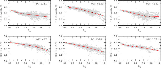
Figure 3: Examples of the abundance distributions in the discs of spiral galaxies. The grey points depict the abundances in individual regions (spaxels in the CALIFA survey). The dashed (black) line shows the pure linear fit to those data. The solid (red) line represents the broken linear fit.

Simple calibration relations for abundances from a set of strong emission lines were suggested (Pilyugin & Grebel 2016). Using these relations, the oxygen abundances are determined using the $N_{2}$ = 1.33[N ii]$\lambda$6584/H$\beta$, $R_{3}$ = 1.33[O iii]$\lambda$5007/H$\beta$, and $S_{2}$ = ([S ii]$\lambda$6717 + [S ii]$\lambda$6731)/H$\beta$ line ratios

$$\begin{array}[]{lll}{\rm(O/H)}^{*}&=&8.424+0.030\,\log(R_{3}/S_{2})+0.751\,\log N_{2}\\ &+&(-0.349+0.182\,\log(R_{3}/S_{2})+0.508\log N_{2})\\ &\times&\log S_{2}\\ \end{array}$$ (6)

if log$N_{2}>-0.6$, and

$$\begin{array}[]{lll}{\rm(O/H)}^{*}&=&8.072+0.789\,\log(R_{3}/S_{2})+0.726\,\log N_{2}\\ &+&(1.069-0.170\,\log(R_{3}/S_{2})+0.022\log N_{2})\\ &\times&\log S_{2}\\ \end{array}$$ (10)

if log$N_{2}\leq-0.6$. The notation (O/H)^∗ = 12 +log(O/H) is used for sake of brevity.

This calibration provides estimates of the oxygen abundances with high precision over the whole metallicity scale. The mean difference between the calibration-based and $T_{e}$-based oxygen abundances is around 0.05 dex (Pilyugin & Grebel 2016). Thus our metallicity scale is well compatible with the metallicity scale defined by the $T_{e}$-based oxygen abundances.

3.2 Fits to radial abundance distribution

Two different fits to the radial oxygen abundance distribution are considered. First, we fit the radial oxygen abundance distribution in each galaxy by the traditional, purely linear relation,

$$12+\log{\rm(O/H)}_{PLR}=12+\log{\rm(O/H)}_{0}+grad\,\times\,R_{g},$$ (11)

where 12 + log(O/H)₀ is the extrapolated central oxygen abundance, $grad$ is the slope of the oxygen abundance gradient expressed in terms of dex/$R_{\rm 25}$, and $R_{g}$ is the fractional radius (the galactocentric distance normalized to the disc isophotal radius).

If there are points that show large deviations from the O/H – $R_{g}$ relation, $d_{OH}>0.3$ dex, then those points are not used in deriving the final relations and are excluded from further analysis. It should be noted that points with such large deviations exist only in some galaxies and those points are both few in number and their deviations exceed 5 – 10$\sigma_{OH}$ (see below). The mean deviation from the final relations (the mean value of the residuals of the relations) is given by the expression

$$\sigma_{OH}=\left(\frac{1}{n}\sum_{j=1}^{n}(\log({\rm O/H})^{OBS}_{j}-\log({\rm O/H})^{CAL}_{j})^{2}\right)^{1/2},$$ (12)

where (O/H)${}_{j}^{CAL}$ is the oxygen abundance computed through Eq. (11) for the galactocentric distance of the $j$-th spaxel and (O/H)${}_{j}^{OBS}$ is the measured oxygen abundance that is obtained through the calibration from the set of emission lines in the spectrum of the $j$-th spaxel. The value of $\sigma_{OH}$ is usually low, from $\sigma_{OH}\sim 0.03$ to $\sigma_{OH}\sim 0.06$ dex (see Fig. 2), and does not depend on the number of data points in the abundance map of a galaxy. This suggests that the typical amplitude of the variation in the oxygen abundance at a given galactocentric distance is rather small.

We also fit the radial oxygen abundance distribution in each galaxy by a broken linear relation,

$$\begin{array}[]{lll}12+\log{\rm(O/H)}_{BLR}&=&a_{1}\,\times\,R_{g}+b_{1},\;\;\;\;\mbox{ if}\;\;R_{g}<R_{b}\\ &=&a_{2}\,\times\,R_{g}+b_{2},\;\;\;\;\mbox{ if}\;\;R_{g}\geq R_{b}\\ \end{array},$$ (15)

where $R_{b}$ is the break radius, $b_{1}$ is the extrapolated central oxygen abundance, $a_{1}$ is the slope of the oxygen abundance gradient expressed in terms of dex/$R_{\rm 25}$ for the points in the inner part of a galaxy, $b_{2}$ is the extrapolated central oxygen abundance, and $a_{2}$ is the slope of the oxygen abundance gradient for the point in the outer part of a galaxy. The values of $R_{b}$, $b_{1}$, $a_{1}$, $b_{2}$, and $a_{2}$ are derived using the requirement that the mean deviations (Eq. 12) from the relation given by Eq. 15 are minimized.

When determining the break in the radial abundance gradient at very small galactocentric distances (near the centre of a galaxy) the following problem may occur. The gradient based on a small range of galactocentric distances or/and on a small number of points can be unreliable. Even a few points with reduced (enhanced) abundances near the centre can result in a (false) break if the (false) break radius $R_{b}$ is small and the number of points within $R_{b}$ is small. The determination of the break in the radial abundance gradient at very large galactocentric distances (near the optical radius $R_{25}$) can also encounter the same problem. To avoid this problem we used the additional requirements that both the inner and outer gradients must be based on at least 50 data points that cover a range of galactocentric distances larger than $0.2R_{25}$. Those additional conditions may result in an underestimation or overestimation of the slope of the inner (outer) gradients in some galaxies as well as shift the position of the small break radius ($R_{b}<0.2R_{25}$) to the $R_{b}=0.2R_{25}$ and the position of the large break radius ($R_{b}>0.8R_{25}$) to $R_{b}=0.8R_{25}$.

Fig. 3 shows prototypical examples of abundance distributions in galactic discs. The grey points in each panel indicate the abundances in individual regions (spaxels) estimated from the CALIFA survey spectra. The dashed (black) line depicts a purely linear fit to those data while the solid (red) line shows a broken linear fit to the data.

3.3 On the validity of radial abundance distributions

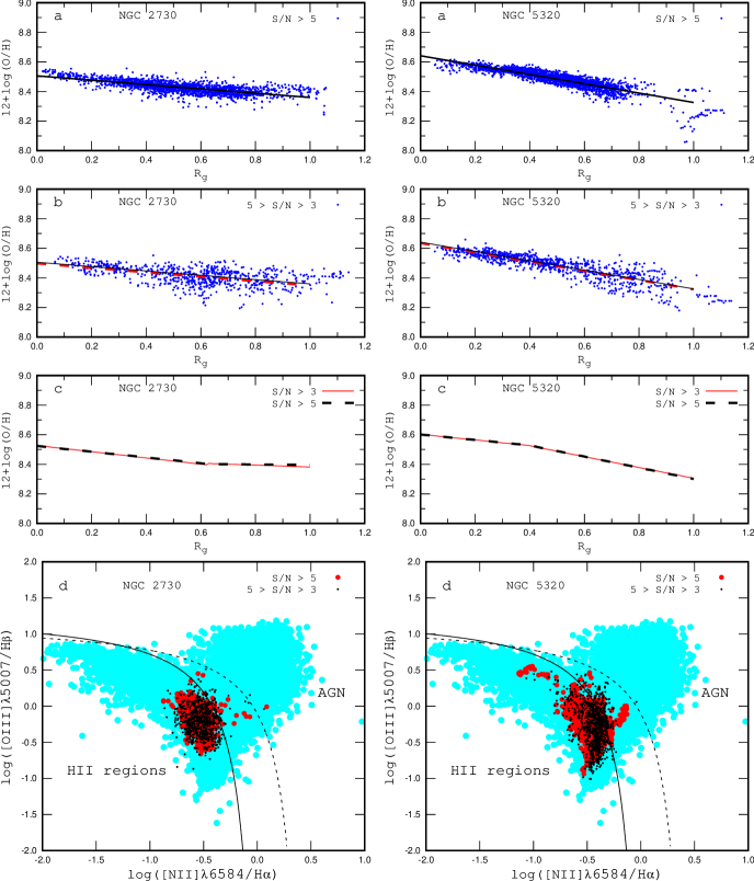
Figure 4: Left column panel shows the properties of the galaxy NGC 2730. Panel $a$ shows the radial abundance distributions traced by spaxels with high-quality spectra, i.e. with a S/N $>$ 5 for each of the measured emission lines. The points depict individual spaxels. The dark (black) solid line is the linear best fit to those data. Panel $b$ shows the radial abundance distributions traced by the spaxels with moderate-quality spectra, i.e. with a 5 $>$ S/N $>$ 3 for each of the measured emission lines. The points denote individual spaxels, the dark grey (red) dashed line is the pure linear best fit to those data, and the dark (black) solid line is the same as in panel $a$. Panel $c$ shows the comparison between the broken linear fits to the data for the specta with S/N $>$ 3 (dark grey (red) solid line) and for the spectra with S/N $>$ 5 (dark (black) dashed line). Panel $d$ shows the classification [N ii]$\lambda$6584/H$\alpha$ vs. [O iii]$\lambda$5007/H$\beta$ diagram. The dark grey (red) points indicate the spaxels with high-quality spectra. The dark (black) points stand for the spaxels with moderate-quality spectra. The solid line separates objects with H ii spectra from those containing an AGN according to Kauffmann et al. (2003), while the dashed line is the same boundary according to Kewley et al. (2001). The grey (light blue) filled circles show a large sample of emission-line SDSS galaxies (Thuan al. 2010). The right column panels show the same but for the galaxy NGC 5320.

Figure 5: Scatter of the oxygen abundances $\sigma_{OH,PLR}$ around the purely linear relation O/H – $R_{g}$ as a function of galaxy inclination (upper panel) and central oxygen abundance (lower panel).

As noted above, we included all spaxel spectra in the analysis where the ratio of the flux to the flux error, S/N $>$ 3, for each of the lines used in the abundance determinations. If the number of the spaxel spectra with measured emission lines in a given galaxy is large enough then the influence of the adopted level of the S/N of the line measurement on the parameters of the abundance distribution can be investigated.

The left column panels of Fig. 4 show the properties of the galaxy NGC 2730, where the gradient in the outer part of the disc is flatter than that in the inner part. Panel $a$ shows the radial abundance distributions traced by spaxels with high-quality spectra, i.e. a S/N $>$ 5 for each of the measured emission lines. The points stand for individual spaxels. The solid (black) line is the purely linear best fit to those data. Panel $b$ shows the radial abundance distributions traced by spaxels with moderate-quality spectra, i.e. with a 5 $>$ S/N $>$ 3 for each of the measured emission lines. The points denote individual spaxels, the dashed (red) line is the purely linear best fit to those data, and the solid (black) line is the same as in the panel $a$. Panel $c$ shows the comparison between the broken linear fits to the data for specta with S/N $>$ 3 (solid (red) line) and for spectra with S/N $>$ 5 (dashed (black) line). There is a remarkable agreement between those fits. Panel $d$ shows the [N ii]$\lambda$6584/H$\alpha$ versus [O iii]$\lambda$5007/H$\beta$ classification diagram. The red points indicate spaxels with high-quality spectra. The black points indicate spaxels with moderate-quality spectra. The solid line separates objects with H ii region spectra from those containing an AGN according to Kauffmann et al. (2003), while the dashed line is the boundary line according to Kewley et al. (2001). The light blue points show a large sample of emission-line SDSS galaxies (Thuan al. 2010). The right column panels of Fig. 4 show the same but for the galaxy NGC 5320, where the gradient in the inner part of the disc is flatter than that in the outer part.

Inspection of panels $a$ and $b$ of Fig. 4 shows that both the spaxels with high-quality spectra as well as the spaxels with moderate-quality spectra are distributed across the whole extent of the discs of both galaxies. Panels $d$ in Fig. 4 show that the spaxels with moderate-quality spectra occupy the same area in the diagnostic [N ii]$\lambda$6584/H$\alpha$ versus [O iii]$\lambda$5007/H$\beta$ diagram as the spaxels with high-quality spectra.

A comparison between the left column panels $a$ and $b$ of Fig. 4 shows that the purely linear gradient in the disc of the galaxy NGC 2730 traced by spaxels with high-quality spectra (1883 data points) is in agreement with the purely linear gradient traced by the spaxels with moderate-quality spectra (718 data points). However, the scatter of the abundances in spaxels with high-quality spectra around the O/H – $R_{g}$ relation, $\sigma_{\rm OH,PLR}=0.0283$, is lower than that for the spaxels with moderate-quality spectra, $\sigma_{\rm OH,PLR}=0.0510$. A similar behaviour is seen in the galaxy NGC 5320 (right column panels $a$ and $b$ of Fig. 4). While the purely linear gradients traced by the spaxels with high-quality spectra (2045 data points) and by the spaxels with moderate-quality spectra (890 data points) are in agreement, the scatter of the abundances in spaxels with high-quality spectra around the O/H – $R_{g}$ relation, $\sigma_{\rm OH,PLR}$ = 0.0297, is lower than that for the spaxels with moderate-quality spectra, $\sigma_{\rm OH,PLR}$ = 0.0410. The left and right column panels $c$ show that the broken linear O/H – $R_{g}$ relation traced by the spaxels with high-quality spectra agrees with relation traced by all the spaxels (i.e. the spaxels with high-quality spectra and spaxels with moderate-quality spectra taken together).

Thus, the use of spaxel spectra with a S/N $>$ 3 for each of the lines used in the abundance determinations is justified and does not influence the derived characteristics of the abundance distribution, i.e. the slope of the gradient and the break in the abundance distribution, although it increases the scatter around the O/H – $R_{g}$ relation. This result is not surprising since the condition S/N $>$ 3 is the standard criterion and has been widely used for a long time.

Our sample involves a number of galaxies with large inclinations, $i>70{\degr}$ (see panel $e$ in Fig. 1). One can expect that the deprojected galactocentric distances of the spaxels in galaxies with large inclinations may suffer from large uncertainties that can result in an increase of the scatter around the O/H – $R_{g}$ relation. Fig. 5 shows the scatter of the oxygen abundances $\sigma_{OH,PLR}$ around the purely linear relation O/H – $R_{g}$ as a function of galaxy inclination (upper panel) and central oxygen abundance (lower panel). The upper panel of Fig. 5 shows that the value of the scatter $\sigma_{OH,PLR}$ is not correlated with the inclination. This suggests that a reliable O/H – $R_{g}$ diagram can be obtained even for galaxies with a large inclination, up to $i\sim 80{\degr}$.

Inspection of the lower panel of Fig. 5 shows that there is a correlation between the value of the oxygen abundance scatter $\sigma_{OH,PLR}$ and the (central) oxygen abundance in the sense that the scatter increases with decreasing oxygen abundance. This could have the following cause. The flux in the nitrogen emission line [N ii]$\lambda$6584, which plays a significant role in the abundance determinations decreases with decreasing galaxy metallicity. This can result in an increase of the uncertainties in the measurements of the [N ii]$\lambda$6584 emission-line fluxes with decreasing galaxy metallicity and, as a consequence, may lead to an increase of the oxygen abundance scatter with decreasing abundance. It also cannot be excluded that the real scatter in the abundances is large in the less evolved (lower abundance and astration level) galaxies than in the more evolved (higher abundance and astration level) galaxies. If this is the case then this effect may contribute to the observed trend $\sigma_{OH,PLR}$ – O/H.

3.4 Properties of radial abundance distributions

Figure 6: Scatter of oxygen abundances $\sigma_{OH,BLR}$ around broken linear relation O/H – $R_{g}$ vs. scatter $\sigma_{OH,PLR}$ around the purely linear relation. The dashed line indicates unity.

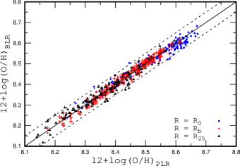
Figure 7: Comparison between oxygen abundances (O/H)_PLR given by the purely linear relation (O/H) – $R_{g}$ and abundances (O/H)_BLR given by the broken linear relation at the galaxy centres (circles), at the break radii (plus signs), and at the optical radii $R_{25}$ (triangles) of the galaxies. The solid line indicates equal values. The two dashed lines show the $\pm 0.05$ dex deviations from unity.

Figure 8: Normalized histogram of the ratios of the difference between broken and linear relation O/H – $R_{g}$ to the abundance scatter around the broken relation $\Delta$(O/H)_BLR,PLR/$\sigma_{OH,BLR}$ for our sample of galaxies.

Table 1: Break radii in $R_{g}$ – (O/H)_X relations for oxygen abundances (O/H)_X determined through different calibrations: the (O/H)_PG16 abundances were determined using the $S$ calibration of Pilyugin & Grebel (2016), whereas the (O/H)_M13,O3N2 and (O/H)_M13,N2 abundances were obtained through the O3N2 and N2 calibrations of Marino et al. (2013), respectively. The break radii are fractional radii, i.e. they are normalized to the optical radii.

	break radius in $R_{g}$ – (O/H)X relation
Galaxy	(O/H)PG16	(O/H)M13,O3N2	(O/H)M13,N2
NGC 0477	0.71	0.35	0.69
NGC 0768	0.55	0.55	0.39
NGC 3811	0.46	0.47	0.34
NGC 4644	0.80	0.48	0.80
NGC 4961	0.67	0.57	0.61
NGC 5320	0.40	0.41	0.50
NGC 5630	0.53	0.53	0.54
NGC 5633	0.47	0.27	0.55
NGC 5980	0.77	0.49	0.80
NGC 6063	0.75	0.40	0.77
NGC 6186	0.40	0.58	0.37
NGC 6478	0.76	0.47	0.70
NGC 7364	0.42	0.20	0.24
NGC 7489	0.33	0.31	0.28
NGC 7631	0.67	0.55	0.45
IC 0480	0.76	0.32	0.76
IC 1151	0.76	0.28	0.79
IC 2098	0.78	0.50	0.50
UGC 00005	0.44	0.29	0.64
UGC 00841	0.34	0.32	0.60
UGC 01938	0.42	0.48	0.42
UGC 02319	0.79	0.80	0.79
UGC 04029	0.73	0.60	0.79
UGC 04132	0.79	0.38	0.53
UGC 09665	0.74	0.70	0.80
UGC 12857	0.80	0.80	0.80

It is evident that any radial abundance distribution is fitted better by the broken linear relation than by the purely linear relation. The general difference between pure and broken linear relations can be specified by the difference of the scatter of the abundances around those relations and by the maximum difference between the abundances given by those relations.

Fig. 6 shows the scatter of the oxygen abundances $\sigma_{OH,BLR}$ around the broken linear relation O/H – $R_{g}$ versus the scatter $\sigma_{OH,PLR}$ around the purely linear relation. The circles show individual galaxies. The dashed line is that of equal values. Fig. 6 illustrates that the scatter of the oxygen abundances $\sigma_{OH,BLR}$ is very close to the scatter $\sigma_{OH,PLR}$. The difference between those values is negligibly small in the majority of our galaxies.

The difference between the broken and purely linear (O/H) – $R_{g}$ relations can be specified in the following way. The difference between the abundance (O/H)_BLR corresponding to the broken (O/H) – $R_{g}$ relation and the abundance (O/H)_PLR corresponding to the purely linear (O/H) – $R_{g}$ relation is defined as $\Delta$(O/H)_BLR,PLR($R_{g}$) = log(O/H)_BLR($R_{g}$) - log(O/H)_PLR($R_{g}$) and changes in radial direction. The maximum difference occurs either at the centre of a galaxy, break radius $R_{b}$, or optical isophotal radius $R_{25}$.

Fig. 7 shows the oxygen abundance (O/H)_BLR as a function of the abundance (O/H)_PLR at the centres (circles), break radii (plus signs), and optical radii (triangles) of our galaxies. Since there may be a jump in oxygen abundance at the break radius we are presenting two values of the (O/H)_BLR at the break radius estimated from the gradients of the inner and outer parts of the disc. The solid line is that of equal values; the dashed lines show the $\pm$0.05 dex deviations from unity. Inspection of Fig. 7 shows that the maximum difference between the abundances (O/H)_BLR and (O/H)_PLR is within 0.05 dex for the majority of the galaxies of our sample.

We specify the difference between the broken and purely linear (O/H) – $R_{g}$ relations by the maximum absolute value of the difference. This value is referred to as $\Delta$(O/H)_BLR,PLR below. Fig. 8 shows the normalized histogram of the ratios of the difference between the broken and linear the relation O/H – $R_{g}$ to the abundance scatter around the broken relation $\Delta$(O/H)_BLR,PLR/$\sigma_{OH,BLR}$ for our galaxy sample. Inspection of Fig. 8 shows that the difference between the broken and linear relations exceeds the abundance scatter around the broken relation for 26 galaxies out of 134 objects.

3.5 Breaks in the radial distributions of abundances obtained through various calibrations

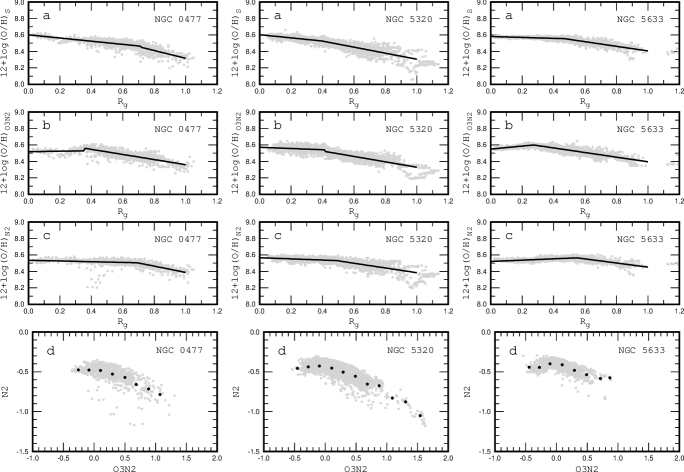
Figure 9: Breaks in the radial distributions of oxygen abundances in discs of three galaxies determined via three different calibrations are depicted. The left column panels show the galaxy NGC 0477, where the break radii in the (O/H)_PG16 and the (O/H)_M13,N2 distributions are close to each other and differ from the break radius obtained from the (O/H)_M13,O3N2 distribution. The grey points in panels $a$, $b$, and $c$ are the data for individual spaxels. The line is the broken linear fit O/H – $R_{g}$ to those data points. Panel $d$ shows the N2 abundance index as a function of the O3N2 index for individual spaxels (grey points) and mean values for bin sizes of 0.2 in O3N2 (dark points). The middle column panels show the galaxy NGC 5320, where the break radii in the (O/H)_PG16 and the (O/H)_M13,O3N2 distributions are close to each other and differ from that in the (O/H)_M13,N2 distribution. The right column panels show the galaxy NGC 5633, where the break radii for the three abundance determination methods are different.

The 1D O3N2 and N2 calibrations suggested by Pettini & Pagel (2004) are widely used for abundance estimations. We aim to find out whether the radial distributions of abundances obtained with those calibrations show breaks in the slopes of their gradients. We found above that the radial distributions of oxygen abundances estimated through the calibration of Pilyugin & Grebel (2016) show a prominent break in the abundance gradients in the discs of 26 galaxies. The oxygen abundances in those galaxies were determined using the recent version of the Pettini & Pagel calibrations suggested by Marino et al. (2013). The (O/H)_M13,O3N2 and (O/H)_M13,N2 abundances were determined using the calibration relations

$$12+\log({\rm O/H})_{\rm M13,O3N2}=8.533-0.214\times{\rm O3N2},$$ (16)

where

$${\rm O3N2}=\log\left(\frac{[{\rm O\leavevmode\nobreak\ III}]\lambda 5007}{{\rm H}\beta}/\frac{[{\rm N\leavevmode\nobreak\ II}]\lambda 6584}{{\rm H}\alpha}\right)$$ (17)

and

$$12+\log({\rm O/H})_{\rm M13,N2}=8.743+0.462\times{\rm N2},$$ (18)

where

$${\rm N2}=\log\left(\frac{[{\rm N\leavevmode\nobreak\ II}]\lambda 6584}{{\rm H}\alpha}\right).$$ (19)

The obtained radial abundance distribution in each galaxy is fitted by a broken linear relation. The break radii in the O/H – $R_{g}$ relations for oxygen abundances determined through the three different calibrations are reported in Table 1; the abundances determined through the $S$ calibration of Pilyugin & Grebel (2016) are referred to as (O/H)_PG16 abundances in this section.

Table 1 shows that the break radii in the (O/H)_PG16 – $R_{g}$ and (O/H)_M13,O3N2 – $R_{g}$ distributions agree within 0.1$R_{25}$ for 11 galaxies, the break radii in the (O/H)_PG16 – $R_{g}$ and (O/H)_M13,N2 – $R_{g}$ distributions agree for 18 galaxies, and the break radii in (O/H)_M13,O3N2 – $R_{g}$ and (O/H)_M13,N2 – $R_{g}$ distributions agree for 10 galaxies. Panels $a$, $b$, and $c$ in Fig. 9 show the breaks in the radial distributions of oxygen abundances in discs of three galaxies determined through three different calibrations. The left column panels show the galaxy NGC 0477 where the break radii in the (O/H)_PG16 and (O/H)_M13,N2 distributions are close to each other, but differ from that in the (O/H)_M13,O3N2 distribution. The middle column panels show the galaxy NGC 5320 where the break radii in the (O/H)_PG16 and (O/H)_M13,O3N2 distributions are close to each other, but differ from that in the (O/H)_M13,N2 distribution. The right column panels show the galaxy NGC 5633 where the break radii in the three distributions are different.

Panels $d$ in Fig. 9 show the N2 abundance index as a function of the O3N2 index for individual spaxels (grey points) and mean values with a bin size of 0.2 in O3N2 (dark points) for the three galaxies. The N2 – O3N2 diagrams for the individual galaxies (panels $d$ in Fig. 9) suggest that the disagreement between the break radii in the O/H – $R_{g}$ relations for oxygen abundances originates in the use of the three different calibrations. Indeed, the relation between O3N2 and the N2 abundance indicators is not strictly linear. Instead there is an appreciable deviation from the linear relation. Hence, the 1D linear expressions O/H = $f$(O3N2) and O/H = $f$(N2) cannot both be correct simultaneously and cannot provide consistent (correct) values of the oxygen abundances over whole interval of the abundance index O3N2 (or the abundance index N2). This may result in a false apparent break in the distribution of abundances produced by one (or both) of the 1D calibrations of the Pettini & Pagel type and, consequently, may lead to the disagreement in the break radii in the distributions of the abundances produced by the O3N2 and N2 calibrations.

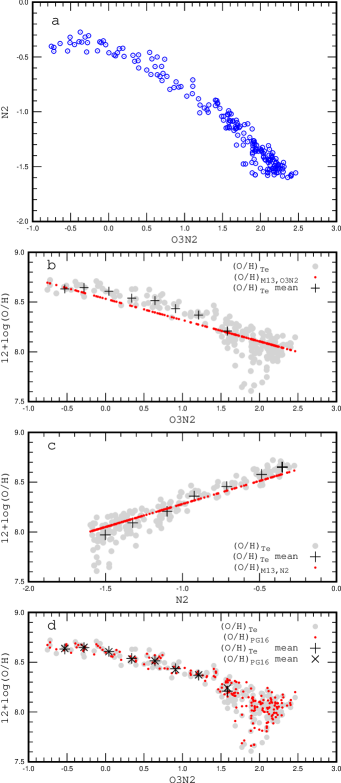
Figure 10: Panel $a$ shows the N2 abundance index as a function of the O3N2 abundance index for objects with $T_{e}$-based abundances (compilation from Pilyugin & Grebel (2016)). Panel $b$ shows the (O/H)${}_{T_{e}}$ abundances (grey points) and the (O/H)_M13,O3N2 abundances (red points) for individual objects, and the mean (O/H)${}_{T_{e}}$ abundances (plus signs) in bins with a width of 0.3 in O3N2 as a function of O3N2. Panel $c$ shows the (O/H)${}_{T_{e}}$ abundances (grey points) and the (O/H)_M13,N2 abundances (red points) for individual objects, and the mean (O/H)${}_{T_{e}}$ abundances (plus signs) in bins with a width of 0.2 in N2 as a function of N2. Panel $d$ shows the (O/H)${}_{T_{e}}$ abundances (grey points) and the (O/H)_PG16 abundances (red points) for individual objects, the mean (O/H)${}_{T_{e}}$ abundances (plus signs) and (O/H)_PG16 abundances (crosses) with a bin width of 0.3 in O3N2 as a function of O3N2.

A sample of objects with $T_{e}$-based abundances has been compiled in Pilyugin & Grebel (2016). The analysis of this sample can tell us something about the validity of the distributions of the abundances determined through the different calibrations and can clarify the origin of the disagreement between the break radii in those distributions. Only objects for which the N2 calibration is applicable (N2 $>-1.6$) are included in the analysis. Panels $a$ in Fig. 10 shows the N2 abundance index as a function of the O3N2 index for a sample of objects with $T_{e}$-based oxygen abundances. A comparison of panels $a$ in Fig. 10 with panels $d$ in Fig. 9 shows that the O3N2 – N2 diagram for objects from Pilyugin & Grebel (2016) also shows an appreciable deviation from the linear relation similar to the O3N2 – N2 diagrams for individual spaxels in each galaxy. Panel $b$ shows the (O/H)${}_{T_{e}}$ abundances (grey points) and the (O/H)_M13,O3N2 abundances (red points) for individual objects, and the mean (O/H)${}_{T_{e}}$ abundances (plus signs) in bins with a width of 0.3 in O3N2 as a function of O3N2. Panel $c$ shows the abundances in (O/H)${}_{T_{e}}$ (grey points) and (O/H)_M13,N2 (red points) for individual objects, and the mean (O/H)${}_{T_{e}}$ abundances (plus signs) in bins with a width of 0.2 in N2 as a function of N2. Panel $d$ shows the abundances in (O/H)${}_{T_{e}}$ (grey points) and (O/H)_PG16 (red points) for individual objects, the mean (O/H)${}_{T_{e}}$ abundances (plus signs), and (O/H)_PG16 abundances (crosses) for a bin width of 0.3 in O3N2 as a function of O3N2.

The comparison between panels $b$ and $c$ of Fig. 10 shows that the N2 calibration can be applied to a larger number of objects than the O3N2 calibration. Indeed, all the selected objects satisfy the criterion of the applicability of the N2 calibration, N2 $>-1.6$ (panel $c$ in Fig. 10). However, some of those objects do not satisfy the criterion of the applicability of the O3N2 calibration, O3N2 $<$ 1.7 (panel $b$ in Fig. 10).

Panel $b$ of Fig. 10 shows that there is an appreciable difference between the (O/H)_M13,O3N2 and (O/H)${}_{T_{e}}$ abundances and the difference changes with the O3N2 index in a nonlinear manner. Therefore the (O/H)_M13,O3N2 – $R_{g}$ and the (O/H)${}_{T_{e}}$ – $R_{g}$ diagrams for the same galaxy can show different slopes of the gradients and breaks at different radii. Inspection of panel $c$ of Fig. 10 shows that there is also a considerable difference between the (O/H)_M13,N2 and (O/H)${}_{T_{e}}$ abundances. However, the difference changes with the N2 index in a linear manner. Therefore the (O/H)_M13,N2 – $R_{g}$ and (O/H)${}_{T_{e}}$ – $R_{g}$ diagrams for the same galaxy can show different slopes of the gradients but they should show breaks (if they exist) at similar radii. Examination of panel $d$ of Fig. 10 shows that the (O/H)_PG16 and (O/H)${}_{T_{e}}$ abundances are in agreement over the whole interval of the O3N2 index. Therefore the (O/H)_PG16 – $R_{g}$ and (O/H)${}_{T_{e}}$ – $R_{g}$ diagrams for the same galaxy can show similar slopes of the gradients and exhibit breaks at the same (or at least quite similar) radii, i.e. the (O/H)_PG16 – $R_{g}$ diagram allows us to determine a reliable slope of the gradients and a reliable value of the break radius.

Thus, the break radius derived from the (O/H)_M13,N2 – $R_{g}$ diagram is more reliable than the break radius obtained from the (O/H)_M13,O3N2 – $R_{g}$ diagram. This explains why the agreement between the values of the break radii in the (O/H)_M13,N2 – $R_{g}$ and (O/H)_PG16 – $R_{g}$ diagrams is better that the agreement between the values of the break radius in the (O/H)_M13,O3N2 – $R_{g}$ and (O/H)_PG16 – $R_{g}$ , or in the (O/H)_M13,O3N2 – $R_{g}$ and the (O/H)_M13,N2 – $R_{g}$, diagrams (see Table 1). Marino et al. (2016) also note that the N2 calibration provides a better match to the abundances obtained through the $T_{e}$ method.

4 Surface brightness profiles

4.1 Bulge-disc decomposition

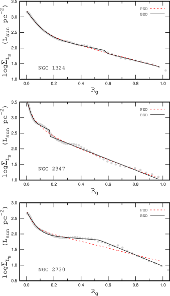
Figure 11: Examples of the observed surface brightness profiles and fits. In each panel, the grey points show the observed surface brightness profile. The dashed (red) line indicates the pure exponential fit to those data. The solid (black) line indicates the broken exponential fit. The upper panel shows the galaxy NGC 1324 with an observed surface brightness profile close to a purely exponential disc. The middle panels shows the galaxy NGC 2347, which exhibits humps and troughs in the observed surface brightness profile. The lower panel shows the galaxy NGC 2730 with a surface brightness profile with a clear break.

Surface brightness measurements in solar units were used for the bulge-disc decomposition. The magnitude of the Sun in the $B$ band of the Vega photometric system, $B_{\sun}=5.45$, was taken from Blanton & Roweis (2007).

The stellar surface brightness distribution within a galaxy was fitted by an exponential profile for the disc and by a general Sérsic profile for the bulge. The total surface brightness distribution was fitted with the expression

$$\begin{array}[]{lll}\Sigma_{L}(r)&=&(\Sigma_{L})_{e}\exp\{-b_{n}[(r/r_{e})^{1/n}-1]\}\\ &+&(\Sigma_{L})_{0}\exp(-r/h),\\ \end{array}$$ (22)

where $(\Sigma_{L})_{e}$ is the surface brightness at the effective radius $r_{e}$, i.e. the radius that encloses 50% of the bulge light, $(\Sigma_{L})_{0}$ is the central disc surface brightness, and $h$ the radial scale length. The factor $b_{n}$ is a function of the shape parameter $n$. This factor can be estimated as $b_{n}\approx 1.9992n-0.3271$ for $1<n<10$ (Graham 2001). The fit via Eq. (22) is referred to below as a purely exponential disc (PED) approximation. It is known that the surface brightnesses in some galaxies are flat or even increase out to a region of slope change where they tend to fall off. Such surface brightness profiles can be formally fitted by an exponential disc with a bulge-like component of negative brightness (Pilyugin et al. 2015).

The parameters $(\Sigma_{L})_{e}$, $r_{e}$, $n$, $(\Sigma_{L})_{0}$, and $h$ are obtained through the best fit to the observed radial surface brightness profile, i.e. we derive a set of parameters in Eq. (22) that minimizes the deviation $\sigma_{PED}$ of

$$\sigma=\sqrt{[\sum\limits_{j=1}^{n}(L(r_{j})^{cal}/L(r_{j})^{obs}-1)^{2}]/n}.$$ (23)

Here $L(r_{j})^{cal}$ is the surface brightness at the radius $r_{j}$ computed through Eq. (22) and $L(r_{j})^{obs}$ is the measured surface brightness at that radius.

The stellar surface brightness distribution within a galaxy was also fitted with the broken exponential

$$\begin{array}[]{lll}\Sigma_{L}(r)&=&(\Sigma_{L})_{e}\exp\{-b_{n}[(r/r_{e})^{1/n}-1]\}\\ &+&(\Sigma_{L})_{0,inner}\exp(-r/h_{inner})\;\;\;\;if\;\;\;r<R^{*},\\ &=&(\Sigma_{L})_{e}\exp\{-b_{n}[(r/r_{e})^{1/n}-1]\}\\ &+&(\Sigma_{L})_{0,outer}\exp(-r/h_{outer})\;\;\;\;if\;\;\;r>R^{*}.\\ \end{array}$$ (28)

Here $R^{*}$ is the break radius, i.e. the radius at which the exponent changes. The fit via Eq. (28) is referred to below as the broken exponential disc (BED) approximation. Again, eight parameters $(\Sigma_{L})_{e}$, $r_{e}$, $n$, $(\Sigma_{L})_{0,inner}$, $h_{inner}$, $(\Sigma_{L})_{0,outer}$, $h_{outer}$, and $R^{*}$ in the broken exponential disc were determined through the best fit to the observed surface brightness profile, i.e. we again require that the deviation $\sigma_{BED}$ given by Eq. (23) is minimized.

4.2 Breaks in the surface brightness profiles

Figure 12: In the upper panel the scatter of the surface brightness $\sigma_{SB,BED}$ around the broken exponential fit vs. the scatter $\sigma_{SB,PED}$ around the pure exponential fit is plotted. The dashed line indicates equal values. The lower panel shows the normalized histogram of the scatter ratios $\sigma_{SB,BED}$/$\sigma_{SB,PED}$ for our sample of galaxies.

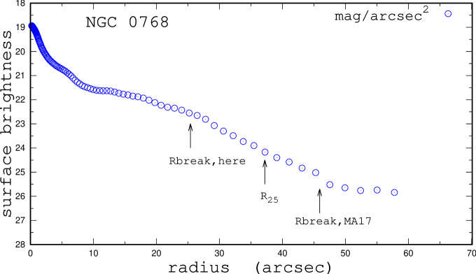
Figure 13: Observed surface brightness profile of the galaxy NGC 0768 in the $g$ SDSS photometric band (points). The optical radius $R_{25}$ and the breaks in the surface brightness distribution obtained here and by Méndez-Abreu et al. (2017) are shown with the arrows.

Fig. 11 shows examples of the surface brightness profiles of our sample of galaxies. The grey points are the observed surface brightness profiles. The dashed (red) line is the purely exponential fit to those data, the solid (black) line is the broken exponential fit. The upper panel of Fig. 12 shows the scatter of the surface brightnesses $\sigma_{SB,BED}$ around the broken exponential disc profile as a function of scatter $\sigma_{SB,PED}$ around the pure exponential disc profile. The circles stand for individual galaxies. The dashed line indicates equal values.

The upper panel of Fig. 11 shows the measured surface brightness profile of the galaxy NGC 1324, which is an example of a galaxy with a surface brightness profile close to a pure exponential disc. The pure and broken exponential disc fits are close to each other. The scatter in the surface brightnesses around the pure and broken exponential disc profiles are rather small for those galaxies. These galaxies are located near the line of equal values in the $\sigma_{SB,BED}$ – $\sigma_{SB,PED}$ diagram, Fig. 12, at low values of $\sigma_{SB,BED}$ and $\sigma_{SB,PED}$. The scatter ratio $\sigma_{SB,BED}$/$\sigma_{SB,PED}$ for those galaxies is close to 1.

The middle panel of Fig. 11 shows the measured surface brightness profile of the galaxy NGC 2347, which is an example of a galaxy with humps and troughs in the observed surface brightness profile. This may be a result of spiral arms or other structures. The scatter in the surface brightnesses both around the pure and broken exponential disc profiles is large for those galaxies but the deviation of the scatter ratio $\sigma_{SB,BED}$/$\sigma_{SB,PED}$ from 1 is not very large. These galaxies are located near the line of equal values in the $\sigma_{SB,BED}$ – $\sigma_{SB,PED}$ diagram, Fig. 12, at large values of $\sigma_{SB,BED}$ and $\sigma_{SB,PED}$.

The lower panel of Fig. 11 shows the measured surface brightness profile of the galaxy NGC 2730, which is an example of a galaxy where the surface brightness profile shows a prominent break. The purely exponential disc is in significant disagreement with the observed surface brightness profile; the value of the scatter $\sigma_{SB,PED}$ is high. In contrast, the broken exponential disc adequately reproduces the observed surface brightness profile, and the value of the scatter $\sigma_{SB,BED}$ is low. The scatter ratio $\sigma_{SB,BED}$/$\sigma_{SB,PED}$ for those galaxies is significantly less than 1. These galaxies are located much below the line of equal values on the $\sigma_{SB,BED}$ – $\sigma_{SB,PED}$ diagram, Fig. 12, both at low and high values of $\sigma_{SB,PED}$.

Thus, the scatter ratio $\sigma_{SB,BED}$/$\sigma_{SB,PED}$ for a galaxy can be considered as an indicator of the presence of a break in its surface brightness profile. The lower panel of Fig. 12 shows the normalized histogram of the scatter ratios $\sigma_{SB,BED}$/$\sigma_{SB,PED}$ for our sample of galaxies. One can see that the $\sigma_{SB,BED}$/$\sigma_{SB,PED}$ ratio in a number of galaxies is significantly lower than 1. The $\sigma_{SB,BED}$/$\sigma_{SB,PED}$ ratio can serve as an indicator of the strength of the break in the surface brightness profile. Galaxies with $\sigma_{SB,BED}$/$\sigma_{SB,PED}$ less than 0.6 in their surface brightness profiles are referred to as galaxies with a prominent break in their surface brightness profiles. Certainly, the choice of the value of 0.6 is somewhat arbitrary.

It should be emphasized that the surface brightness distributions within the optical radii of galaxies are only considered and fitted in our current study. Recently, Méndez-Abreu et al. (2017) presented a 2D multi-component photometric decomposition of 404 CALIFA galaxies in the $g$, $r$, and $i$ SDSS bands. These authors considered the surface brightness distributions well beyond the optical radii of these galaxies. Fig. 13 shows the observed surface brightness profile of the galaxy NGC 0768 in $g$ SDSS band using point symbols. The optical radius $R_{25}$ and the breaks in the surface brightness distribution obtained here and by Méndez-Abreu et al. (2017) are shown with arrows. Fig. 13 illustrates that breaks at different radii can be found if the surface brightness profile is considered and fitted to the different limits of the galactocentric distances.

4.3 Relation of breaks in surface brightness profiles and abundance gradients

Figure 14: Panel $a$ shows the difference between the broken and linear relation $\Delta$(O/H)_BLR,PLR/$\sigma_{OH,BLR}$ (indicator of the strength of break in the O/H distribution) as a function of $\sigma_{SB,BED}$/$\sigma_{SB,PED}$ (indicator of the strength of the break of the surface brightness profile). Panel $b$ shows of the difference between abundance gradients on different sides of the break in the abundance distribution as a function of the ratio of the disc scale lengths on different sides of the break in the surface brightness profile. Panel $c$ shows the break radius of the radial oxygen abundance gradient $R_{b,OH}$ vs. the break radius of the surface brightness profile $R_{b,SB}$. Galaxies with a $\Delta$(O/H)_BLR,PLR/$\sigma_{OH,BLR}$ ratio larger than 1 (with a clear break in the radial abundance gradient) are plotted with circles. Galaxies with a $\sigma_{SB,BED}$/$\sigma_{SB,PED}$ ratio less than 0.6 (with a prominent break in the surface brightness profile) are indicated by plus signs. The break radii are normalized to the isophotal radii $R_{25}$ of the galaxies.

Figure 15: Comparison between the shapes of surface brightness profile and abundance gradient in galactic discs. The grey points show the observed surface brightnesses (abundances). The dashed (red) line is the purely exponential (linear) fit to those data, the solid (black) line is the broken exponential (linear) fit. NGC 3815 and UGC 3969 are examples of galaxies where the surface brightness profile is well fitted by a purely exponential disc and the abundance gradient is well described by a purely linear relation. UGC 841 and UGC 7145 are examples of galaxies where the surface brightness profile is well fitted by a purely exponential disc but the abundance gradient shows a prominent break. NGC 6155 and PGC 64373 are examples of galaxies where the surface brightness profile shows an appreciable break while the abundance gradient is well described by a purely linear relation. IC 1151, UGC 5, and NGC 2730 are examples of galaxies where both the surface brightness profile and the abundance gradient display a prominent break.

The break in both the surface brightness profile and abundance distribution in the disc of a galaxy is specified by three caracteristics: the strength (significance) of the break; the type of the break, i.e. the character of the change in the slope of the distribution when passing the break; and by the break radius. If the breaks in the surface brightness profile and abundance gradient in the disc of a galaxy are related then one may expect that the shapes of the surface brightness profiles and abundance gradients in the galactic discs should be similar in the sense that galaxies with a prominent break in the surface brightness profile should also display a prominent break in the radial abundance gradient of the same type, and the position of the break in the surface brightness profile should coincide with the position of the break in the radial abundance gradient.

Panel $a$ in Fig. 14 shows the difference between the broken and linear relation $\Delta$(O/H)_BLR,PLR/$\sigma_{OH,BLR}$ , which is an indicator of the strength of break in the radial abundance distribution, as a function of the $\sigma_{SB,BED}$/$\sigma_{SB,PED}$ ratio, which is an indicator of the break strength in the surface brightness profile). There is no correlation between the strength of the break in the radial abundance distribution and the strength of the break in the surface brightness profile. A prominent break in the surface brightness profile (low value of the $\sigma_{SB,BED}$/$\sigma_{SB,PED}$ ratio) can be accompanied by a break of different strengths in the radial abundance distribution, and the weak break in the radial abundance distribution (low value of the $\Delta$(O/H)_BLR,PLR/$\sigma_{OH,BLR}$) can take place in galaxies with both strong and weak breaks in the surface brightness profiles.

Panel $b$ in Fig. 14 shows the difference between abundance gradients on different sides of the break in the abundance distribution as a function of the ratio of the disc scale lengths on different sides of the break in surface brightness profile. The value of the $grad_{outer}$ – $grad_{inner}$ specifies the type of the break in the radial abundance profile. The positive value of the difference $grad_{outer}$ – $grad_{inner}$ shows that the gradient becomes flatter in going through the break point (up-bending radial abundance profile or looking-down break). The negative value of the difference $grad_{outer}$ – $grad_{inner}$ shows that the gradient becomes steeper in going through the break point (down-bending radial abundance profile or looking-up break). The ratio $h_{outer}$/$h_{inner}$ specifies the type of the break in the surface brightness profile. A ratio $h_{outer}$/$h_{inner}$ lower than 1 means that the surface brightness profile steepens in going through the break point (down-bending surface brightness profile or looking-up break). A ratio $h_{outer}$/$h_{inner}$ higher than 1 means that the surface brightness profile flattens in going through the break point (up-bending surface brightness profile, or looking-down break). Inspection of panel $b$ in Fig. 14 shows that there is no correlation between the type of break in the radial abundance distribution and the type of break in the surface brightness profile. Indeed the down-bending surface brightness profile can be accompanied by a down-bending or by an up-bending radial abundance profile, and a down-bending radial abundance profile can be accompanied by both down-bending and up-bending surface brightness profiles.

Panel $c$ in Fig. 14 shows the break radius of the radial oxygen abundance gradient $R_{b,OH}$ versus the break radius of the surface brightness profiles $R_{b,SB}$. Galaxies with a $\Delta$(O/H)_BLR,PLR/$\sigma_{OH,BLR}$ ratio larger than 1 (with a clear break in the radial abundance gradient) are shown by circles. Galaxies with a $\sigma_{SB,BED}$/$\sigma_{SB,PED}$ ratio less than 0.6 (with a prominent break in the surface brightness profile) are indicated by plus signs. The break radii are normalized to the isophotal radii $R_{25}$ of the galaxies. Inspection of panel $c$ in Fig. 14 shows that there is no correlation between the break radius of the radial oxygen abundance gradient $R_{b,OH}$ and the break radius of the surface brightness profiles $R_{b,SB}$.

Fig. 15 shows examples of galaxies with different shapes of the surface brightness profiles and abundance gradients. The grey points denote the observed surface brightnesses (abundances). The dashed (red) line is the purely exponential (linear) fit to those data, the solid (black) line represents the broken exponential (linear) fit. The galaxies NGC 3815 and UGC 3969 are examples of galaxies where the surface brightness profile of the disc is close to a purely exponential disc, i.e. the profile is well fitted by a purely exponential disc, and the abundance gradient is well described by a purely linear relation. The galaxies UGC 841 and UGC 7145 are examples of galaxies where the surface brightness profile is well fitted by a purely exponential disc but the abundance gradient shows a prominent break. Thus, the purely exponential profile of the surface brightness may be accompanied by either a pure or a broken linear profile of the radial oxygen abundance distribution.

The galaxies NGC 6155 and PGC 64373 in Fig. 15 are examples of galaxies where the surface brightness profile shows an appreciable break while the abundance gradient is well described by a purely linear relation. The galaxies IC 1151, UGC 5, and NGC 2730 are examples of galaxies where both the surface brightness profile and abundance gradient display a prominent break.

Thus, the shape of the surface brightness profile in the disc is not related to the shape of the radial abundance gradient. The broken exponential profile of the surface brightness in the disc can be accompanied by either a pure or broken linear profile of the radial oxygen abundance distribution. And vice versa, a purely exponential profile of the surface brightnes can be accompanied by a pure or by a broken linear profile of the radial oxygen abundance distribution. A break in the surface brightness profile need not be accompanied by a break in the radial abundance gradient. The shape of the surface brightness profile is thus independent of the shape of the radial abundance gradient.

Marino et al. (2016) have compared the abundance gradients in the inner and outer disc parts divided by the break in the surface brightness profile for the CALIFA galaxies. They do not derive the break radius in the abundance gradient through a direct fit of the radial abundance distribution by the broken relation. This prevents us from comparing our results with their results.

5 Discussion

Figure 16: Examples of the abundance distributions in the discs of galaxies with available SDSS spectroscopy. The grey points stand for abundances in individual regions (spaxels) obtained from the CALIFA spectra. The dashed (black) line indicates a purely linear fit to those data; the solid (red) line indicates a broken linear fit. The dark (black) points denote the oxygen abundances determined from the SDSS spectra.

Figure 17: Upper panel: The oxygen abundance (O/H)_SDSS determined from the SDSS spectrum vs. abundance (O/H)_PLR given by the purely linear O/H – $R_{g}$ relation at this radius. The solid line indicates equal values. The dashed lines show the $\pm$0.05 dex deviations from unity. Lower panel: The same as the upper panel but for the (O/H)_BLR given by the broken linear O/H – $R_{g}$ relation.

Spectroscopic measurements of H ii regions in a number of galaxies in our sample are available in the SDSS database. An SDSS spectrum of one region, usually near the centre of the galaxy, is available for around 50 galaxies of our sample, and SDSS measurements of two regions at different galactocentric distances are available in 20 galaxies. This provides an additional possibility to check the validity of the oxygen abundances and radial abundance gradients estimated by us based on CALIFA survey spectroscopy.

The measurements of the emission-line fluxes (H$\beta$, [O iii]$\lambda$5007, H$\alpha$, [N ii]$\lambda$6584, [S ii]$\lambda$6717, and [S ii]$\lambda$6731) in the SDSS spectra and the fiber coordinates were extracted from the SDSS DR12 data (Alam et al. 2015) reported in the ned. The demarcation line of Kauffmann et al. (2003) between H ii region-like and AGN-like objects in the BPT classification diagram of Baldwin et al. (1981) was adopted to select the H ii region-like objects. The dereddening and abundance determinations were carried in the same way as in the case of the CALIFA spectra. The fractional galactocentric distances (normalized to the isophotal radius) of the regions with SDSS spectra were estimated with the geometrical parameters of galaxies obtained here.

Fig. 16 shows examples of the abundance distributions in the discs of galaxies with available SDSS spectra. The grey points denote the oxygen abundances in individual regions (spaxels) determined using the CALIFA survey spectra. The dashed (black) line indicates the purely linear fit to those data; the solid (red) line indicates the broken linear fit. The dark (black) points stand for abundances in individual regions (fibers) estimated from the SDSS spectra. Fig. 16 shows that the abundances derived from the SDSS spectra are in agreement with the abundances obtained from the CALIFA spectra. All the regions with SDSS-based oxygen abundances are located within the bands outlined by the regions with CALIFA-based abundances.

A quantitative comparison between the SDSS-based and CALIFA-based abundances can be performed in the following manner. Using the galactocentric distance of the SDSS fibers, we determined the corresponding abundance (O/H)_PLR given by the purely linear O/H – $R_{g}$ relation at this galactocentric distance and the abundance (O/H)_BLR given by the broken linear O/H – $R_{g}$ relation for that galaxy. The upper panel of Fig. 17 shows the comparison between the (O/H)_SDSS and (O/H)_PLR abundances. The circles stand for the abundances in the individual regions. The solid line indicates equal values. The dashed lines show the $\pm 0.05$ dex deviations from unity. The upper panel of Fig. 17 shows that the SDSS-based abundances are close to the purely linear relation O/H – $R_{g}$ obtained from the CALIFA-based abundances. The deviations of the bulk of the SDSS-based abundances from the CALIFA-based gradients are within 0.05 dex. The lower panel of Fig. 17 shows the comparison between the (O/H)_SDSS and (O/H)_BLR abundances. This panel shows that the SDSS-based abundances are also close to the broken linear relation O/H – $R_{g}$ determined using the CALIFA-based abundances. Again, the deviations of the bulk of the SDSS-based abundances from the CALIFA-based gradients are within 0.05 dex.

Thus the oxygen abundances estimated from the SDSS spectra agree with the abundances obtained from the CALIFA spectra within $\sim 0.05$ dex. This is strong evidence supporting that the use of the spectra of individual spaxels for abundance determinations is justified, our measurements of the line fluxes are reliable, and the criterion $\epsilon\geq 3$ for strong lines to select the spaxels for analysis does not introduce any bias in the determined abundance gradients.

It should be emphasized that in our current study abundance gradients within the optical radii of galaxies are considered. Spectroscopy of H ii regions in the extended discs of several spiral galaxies were carried out by Bresolin et al. (2009); Goddard et al. (2011); Bresolin et al. (2012); Patterson et al. (2012). The radial oxygen abundance gradients in those galaxies were estimated out to around 2.5 times the optical isophotal radius. These authors found that the slope of the radial oxygen abundance gradients changes at the optical radii of their target galaxies, such that beyond the optical radius of the disc the abundance gradients become flatter. In addition, there appears to be an abundance discontinuity close to this transition (Bresolin et al. 2009; Goddard et al. 2011). The change in the gradient slope is more distinct in the radial distribution of nitrogen than in that of oxygen abundances (Pilyugin et al. 2012). Sánchez-Menguiano et al. (2016) found that most of the CALIFA galaxies with reliable oxygen abundance values beyond $\sim$2 effective radii present a flattening of the abundance gradient in these outer regions. They suggest that such flattening seems to be a universal property of spiral galaxies.

It is known that there is a correlation between the local oxygen abundance and stellar surface brightness of a galactic disc (e.g. Webster & Smith 1983; Edmunds & Pagel 1984; Ryder 1995; Moran et al. 2012; Rosales-Ortega et al. 2012; Pilyugin et al. 2014b). If this correlation is local, i.e. there is a point-to-point correlation, then one may expect that the break in the surface brightness profile should be accompanied by a break in the radial abundance gradient. We found in our current study that the shapes of the abundance gradient and surface brightness profile may be different in a given galaxy in the sense that a broken exponential surface brightness profile of a disc may be accompanied by either a pure or broken linear profile of the radial oxygen abundance distribution. Vice versa, a disc with a pure exponential profile of the surface brightness may show either a pure or broken linear profile of the radial oxygen abundance distribution. We also found that there is no correlation between the break radii of the abundance gradient and surface brightness profiles. This suggests that there is no unique point-to-point correlation between local abundance and local surface brightness in the discs of galaxies.

Another argument against a unique point-to-point correlation between the local oxygen abundance and stellar surface brightness in galaxies comes from the following general consideration. By definition, the values of the stellar surface brightness at the optical radius should be very close in all the galaxies. However, the oxygen abundances at the optical radius vary strongly from galaxy to galaxy. The oxygen abundances at the optical radius 12+log(O/H)${}_{R_{25}}$ vary from $\sim$8.1 to $\sim$8.6 for the galaxies of our sample. That is, the variation in the oxygen abundances at the optical radii of different galaxies at a fixed surface brightness is comparable to, or exceeds, the radial variation in the oxygen abundance within a given galaxy; there is a variation of the surface brightness by two to three orders of magnitude. Thus, the comparison of the oxygen abundances at the optical radii of different galaxies provides prominent evidence against a unique point-to-point correlation between the local oxygen abundance and stellar surface brightness. This supports our conclusion that the correlation between the local oxygen abundance and stellar surface brightness is caused by a relation between the global abundance distribution and global surface brightness distribution rather than by a local, point-to-point correlation.

6 Conclusions

We constructed maps of the oxygen abundance in the discs of 134 spiral galaxies using the 2D spectroscopy of the DR3 of the CALIFA survey. The radial abundance gradients within the optical isophotal radii were determined. To examine the existence of a break in the slope of the gradient, the radial oxygen abundance distribution in each galaxy was fitted by a purely linear relation O/H = $f(R_{g}),$ where the commonly accepted logarithmic scale for the oxygen abundance was used, and by a broken linear relation.

Photometric maps of our target galaxies in the $B$ band were constructed using publicly available photometric measurements in the SDSS $g$ and $r$ bands. We carried out bulge-disc decompositions of the obtained surface brightness profiles. The stellar surface brightness distribution across the galaxies was fitted by an exponential profile for the discs and by a general Sérsic profile for the bulges. The surface brightness distribution across the discs was fitted with a pure and a broken exponential.

We found that the maximum absolute difference between the oxygen abundances in a disc given by the broken and purely linear relations is less than 0.05 dex for the majority of our galaxies and exceeds the scatter in abundances for 26 out of 134 galaxies considered. The scatter in abundances around the broken relation is close to the scatter around the purely linear relation; the difference is usually within 5%. Our results suggest that a simple linear relation is adequate to describe the radial oxygen abundance distribution in the discs of spiral galaxies and can be used (at least as the first order approximation) for many tasks.

The breaks in the surface brightness profiles in some galaxies are more prominent; the scatter around the broken exponent is lower by a factor of two and more than that around the pure exponent. The ratio of the scatter around the broken and pure exponential fits can be considered as an indicator of the presence of a break in the surface brightness profile.

The shapes of the surface brightness profile of the disc and its abundance gradient can differ in the sense that the broken exponential profile of the surface brightness in the disc can be accompanied by either a pure or a broken linear profile of the radial oxygen abundance distribution, and vice versa, the pure exponential profile of the surface brightness can be accompanied by either a pure or a broken linear profile of the radial oxygen abundance distribution. We also found that there is no correlation between the break radii of the abundance gradient and surface brightness profiles. Those results demonstrate that a break in the surface brightness profile need not be accompanied by a break in the abundance gradient.

Those results also suggest that there is no unique point-to-point correlation between the local abundance and local surface brightness in the discs of galaxies. A significant variation in the oxygen abundances at the optical radii of different galaxies (at a fixed surface brightness) confirms this conclusion.

References

- Alloin et al. (1979) Alloin D., Collin-Souffrin S., Joly M., Vigroux L., 1979, A&A, 78, 200
- Ahn et al. (2012) Ahn C.P., Alexandroff R., Allende Prieto C., et al., 2012, ApJS, 203, 21
- Alam et al. (2015) Alam, S., Albareti, F. D., Allende Prieto, C., et al. 2015, ApJS, 219, 12
- Andrievsky et al. (2016) Andrievsky S.M., Martin R.P., Kovtyukh V.V., Korotin S.A., Lépine J.R.D., 2016, MNRAS, 461, 4256
- Baldwin et al. (1981) Baldwin J.A., Phillips M.M., & Terlevich R. 1981, PASP, 93, 5
- Belfiore et al. (2017) Belfiore F., Maiolino R., Tremonti C., et al., 2017, MNRAS, 469, 151
- Berg et al. (2015) Berg D.A., Skillman E.D., Croxall K.V., Pogge R.W., Moustakas J., Johnson-Groh M., 2015, ApJ, 806, 16
- Blanton & Roweis (2007) Blanton, M. R., & Roweis, S. 2007, AJ, 133, 734
- Bresolin et al. (2009) Bresolin F., Ryan-Weber E., Kennicutt R.C., Goddard Q., 2009, ApJ, 695, 580
- Bresolin et al. (2012) Bresolin F., Kennicutt R.C., Ryan-Weber E., 2012, ApJ, 750, 122
- Bresolin & Kennicutt (2015) Bresolin F., Kennicutt R.C., 2015, MNRAS, 454, 3664
- Bundy et al. (2015) Bundy K., Bershady M.A., Law D.R., et al., 2015, ApJ, 798, 7
- Croxall et al. (2015) Croxall K.V., Pogge R.W., Berg D.A., Skillman E.D., Moustakas J., 2015, ApJ, 808, 42
- Croxall et al. (2016) Croxall K.V., Pogge R.W., Berg D.A., Skillman E.D., Moustakas J., 2016, ApJ, 830, 4
- de Vaucouleurs (1959) de Vaucouleurs, G., 1959, Handbuch der Physics, 53, 311
- Dinerstein (1990) Dinerstein H. L. 1990, in The Interstellar Medium in Galaxies, ed. H. A Thronson Jr. & J. M. Shull (Astrophysics and Space Science Library, Vol. 161; Dordrecht: Kluwer), 257
- Edmunds & Pagel (1984) Edmunds M.G., Pagel B.E.J., 1984, MNRAS, 211, 507
- Freeman (1970) Freeman K.C., 1970, ApJ, 160, 811
- García-Benito et al. (2015) García-Benito R., Zibetti S., Sánchez S.F., et al., 2015, A&A, 576, A135
- Goddard et al. (2011) Goddard Q.E., Bresolin F., Kennicutt R.C., Ryan-Weber E.V., Rosales-Ortega F.F., 2011, MNRAS, 412, 1246
- Graham (2001) Graham A.W., 2001, AJ, 121, 820
- Gusev et al. (2012) Gusev A.S., Pilyugin L.S., Sakhibov F., Dodonov S.N., Ezhkova O.V., Khramtsova M.S., 2012, MNRAS, 424, 1930
- Ho et al. (2015) Ho I.-T., Kudritzki R.-P., Kewley L.J., Zahid H.J., Dopita M.A., Bresolin F., Rupke D.S.N., 2015, MNRAS, 448, 2030
- Husemann et al. (2013) Husemann B., Jahnke K., Sánchez S.F., et al., 2013, A&A, 549, A87
- Izotov et al. (1994) Izotov Y.I., Thuan T.X., Lipovetsky V.A., 1994, ApJ, 435, 647
- Kauffmann et al. (2003) Kauffmann G., Heckman T.M., Tremonti C., et al. 2003, MNRAS, 346, 1055
- Kennicutt & Garnett (1996) Kennicutt R.C., Garnett D.R., 1996, ApJ, 456, 504
- Kewley et al. (2001) Kewley L.J., Dopita M.A., Sutherland R.S., Heisler C.A., Trevena J. 2001 ApJ, 556, 121
- Makarov et al. (2014) Makarov D., Prugniel P., Terekhova N., Courtois H., Vauglin I., 2014, A&A, 570, A13
- Marino et al. (2013) Marino R.A., Rosales-Ortega F.F., Sánchez S.F., et al., 2013, A&A, 559, A114
- Marino et al. (2016) Marino R.A., Gil de Paz A., Sánchez S.F., et al., 2016, A&A, 585, A47
- Martin & Roy (1995) Martin P., Roy J.-R., 1995, ApJ, 445, 161
- Martin et al. (2015) Martin R.P., Andrievsky S.M., Kovtyukh V.V., Korotin S.A., Yegorova I.A., Saviane I., 2015, MNRAS, 449, 4071
- Méndez-Abreu et al. (2017) Méndez-Abreu J., Ruiz-Lara T., Sánchez-Menguiano L., et al., 2017, A&A, 598, A32
- Moran et al. (2012) Moran S.M., Heckman T.M., Kauffmann G., et al., 2012, ApJ, 745, 66
- Moustakas et al. (2010) Moustakas J., Kennicutt R.C., Tremonti C.A., Dale D.A., Smith J.-D.T., Calzetti D., 2010, ApJS, 190, 233
- Pagel et al. (1979) Pagel B.E.J., Edmunds M.G., Blackwell D.E., Chun M.S., Smith G., 1979, MNRAS, 189, 95
- Patterson et al. (2012) Patterson M.T., Walterbos R.A.M., Kennicutt R.C., Chiappini C., Thilker D.A., 2012, MNRAS, 422, 401
- Paturel et al. (2003) Paturel G., Petit C., Prugniel P., et al., 2003, A&A, 412, 45
- Peng et al. (2010) Peng C.Y., Ho L.C., Impey C.D., Rix H.-W., 2010, AJ, 139, 2097
- Pettini & Pagel (2004) Pettini M., Pagel B.E.J., 2014, MNRAS, 348, L59
- Pilyugin (2001) Pilyugin L.S., 2001, A&A, 373, 56
- Pilyugin (2003) Pilyugin L.S., 2003, A&A, 397, 109
- Pilyugin et al. (2004) Pilyugin L.S., Vílchez J.M., Contini T., 2004, A&A, 425, 849
- Pilyugin et al. (2006) Pilyugin L.S., Thuan T.X., Vílchez J.M., 2006, MNRAS, 367, 1139
- Pilyugin et al. (2007) Pilyugin L.S., Thuan T.X., Vílchez J.M., 2007, MNRAS, 376, 353
- Pilyugin et al. (2012) Pilyugin L.S., Grebel E.K., Mattsson L., 2012, MNRAS, 424, 2316
- Pilyugin et al. (2014a) Pilyugin L.S., Grebel E.K., Kniazev A.Y., 2014a, AJ, 147, 131
- Pilyugin et al. (2014b) Pilyugin L.S., Grebel E.K., Zinchenko I.A., Kniazev A.Y., 2014b, AJ, 148, 134
- Pilyugin et al. (2015) Pilyugin L.S., Grebel E.K., Zinchenko I.A., 2015, MNRAS, 450, 3254
- Pilyugin & Grebel (2016) Pilyugin L.S., Grebel E.K., 2016, MNRAS, 457, 3678
- Pohlen & Trujillo (2006) Pohlen M., Trujillo I., 2006, A&A, 454, 759
- Rosales-Ortega et al. (2012) Rosales-Ortega F.F., Sánchez S.F., Iglesias-Páramo J., et al. 2012, ApJ, 756, L31
- Ryder (1995) Ryder S.D., 1995, ApJ, 444, 610
- Sánchez et al. (2012) Sánchez S.F., Kennicutt R.C., Gil de Paz A., et al., 2012, A&A, 538, A8
- Sánchez et al. (2014) Sánchez S.F., Rosales-Ortega F.F., Iglesias-Páramo J., et al. 2014, A&A, 563, 49
- Sánchez-Menguiano et al. (2016) Sánchez-Menguiano L., Sánchez S.F., Pérez I., et al. 2016, A&A, 587, A70
- Scarano et al. (2011) Scarano S., Lépine J.R.D., Marcon-Uchida M.M., 2011, MNRAS, 412, 1741
- Schlafly & Finkbeiner (2011) Schlafly E. F., & Finkbeiner D. P. 2011, ApJ, 737, 103
- Searle (1971) Searle L. 1971, ApJ, 168, 327
- Smith (1975) Smith H.E. 1975, ApJ, 199, 591
- Storey & Zeippen (2000) Storey P.J., Zeippen C.J., 2000, MNRAS, 312, 813
- Thuan al. (2010) Thuan T.X., Pilyugin L.S., Zinchenko I.A., 2010, ApJ, 712, 1029
- van der Kruit (1979) van der Kruit P.C., 1979, A&AS, 38, 15
- van Zee et al. (1998) van Zee L., Salzer J.J., Haynes M.P., O’Donoghue A.A., Balonek T.J., 1998, AJ, 116, 2805
- Vila-Costas & Edmunds (1992) Vila-Costas M.B., Edmunds M.G. 1992, MNRAS, 259, 121
- Webster & Smith (1983) Webster B.L., Smith M.G., 1983, MNRAS, 204, 743
- York et al. (2000) York D.G., Adelman J., Anderson J.E., et al., 2000, AJ, 120, 1579
- Zahid & Bresolin (2011) Zahid H.J., Bresolin F., 2011, AJ, 141, 192
- Zaritsky (1992) Zaritsky D., 1992, ApJ, 390, L73
- Zaritsky et al. (1994) Zaritsky D., Kennicutt R.C., Huchra J.P., 1994, ApJ, 420, 87
- Zinchenko et al. (2015) Zinchenko I.A., Kniazev A.Y., Grebel E.K., Pilyugin L.S., 2015, A&A, 582, A35
- Zinchenko et al. (2016) Zinchenko I.A., Pilyugin L.S., Grebel E.K., Sánchez S.F., Vílchez J.M., 2016, MNRAS, 462, 2715