On Multistep Stabilizing Correction Splitting Methods with Applications to the Heston Model

Abstract

In this note we consider splitting methods based on linear multistep methods and stabilizing corrections. To enhance the stability of the methods, we employ an idea of Bruno & Cubillos [5] who combine a high-order extrapolation formula for the explicit term with a formula of one order lower for the implicit terms. Several examples of the obtained multistep stabilizing correction methods are presented, and results on linear stability and convergence are derived. The methods are tested in the application to the well-known Heston model arising in financial mathematics and are found to be competitive with well-established one-step splitting methods from the literature.

2000 Mathematics Subject Classification: 65L06, 65M06, 65M20.
Keywords and Phrases: splitting methods, multistep methods, stability, convergence, Heston model.

1 Introduction

In this note we will discuss a class of splitting methods for solving initial value problems for ordinary differential equations (ODEs)

$$u^{\prime}(t)=F(t,u(t))\,,\qquad u(0)=u_{0}\,,$$ (1.1)

with given $u_{0}\in\mathbb{R}^{M}$, $F:\mathbb{R}\times\mathbb{R}^{M}\rightarrow\mathbb{R}^{M}$ and dimension $M\geq 1$. For many problems occurring in practice there is a natural decomposition

$$F(t,u)\,=\,F_{0}(t,u)+F_{1}(t,u)+\cdots+F_{s}(t,u)$$ (1.2)

in which the separate component functions $F_{j}$ are more simple than the whole $F$, and where $F_{0}$ is a non-stiff or mildly stiff term that can be treated explicitly in a time stepping method. For such problems we will study a class of multistep splitting methods with stabilizing corrections, where explicit predictions are followed by corrections that are implicit in one of the $F_{j}$ terms, $j=1,2,\ldots,s$.

1.1 Linear multistep methods with stabilizing corrections

The splitting methods to be considered produce approximations $u_{n}\approx u(t_{n})$ at the step points $t_{n}=n{\mbox{\footnotesize{$\Delta$}}}t$. The methods are based on pairs of linear multistep methods: an implicit method

$$u_{n}\,=\,\sum_{i=1}^{k}a_{i}u_{n-i}+{\mbox{\footnotesize{$\Delta$}}}t\sum_{i=0}^{k}b_{i}F(t_{n-i},u_{n-i})$$ (1.3)

and an explicit one

$$u_{n}\,=\,\sum_{i=1}^{k}\Big{(}a_{i}u_{n-i}+{\mbox{\footnotesize{$\Delta$}}}t\,\widehat{b}_{i}F(t_{n-i},u_{n-i})\Big{)}\,,$$ (1.4)

having the same coefficients $a_{1},a_{2},\ldots,a_{k}$ and the same order $p$.

Starting with an implicit method of order $k$, the matching explicit formula of the same order can be obtained by extrapolation, replacing the implicit term $F(t_{n},u_{n})$ by a linear combination of $F(t_{n-i},u_{n-i})$ terms, $1\leq i\leq k$. More specifically, with $\widehat{c}_{i}=\prod_{j\neq i}\frac{j}{j-i}$, $1\leq i,j\leq k$, it can be seen from the Lagrange interpolation formula that

$$\varphi(t_{n})=\sum_{i=1}^{k}\widehat{c}_{i}\varphi(t_{n-i})+\widehat{C}{\mbox{\footnotesize{$\Delta$}}}t^{k}\varphi^{(k)}(t_{n})+{\cal O}({\mbox{\footnotesize{$\Delta$}}}t^{k+1})$$ (1.5)

for any smooth function $\varphi$, with error constant $\widehat{C}\in\mathbb{R}$. Using this extrapolation procedure to replace the implicit term in (1.3) yields the following coefficients for the explicit method:

$$\widehat{b}_{i}\,=\,b_{i}+b_{0}\widehat{c}_{i}\qquad(i=1,2,\ldots,k)\,.$$ (1.6)

Such a pair of explicit and implicit methods can now be combined to form a splitting method for problems with decomposition (1.2) by using the idea of stabilizing corrections. In each step, first a prediction is made with the explicit method, followed by corrections for the implicit function components $F_{j}$ with $j=1,2,\ldots,s$:

$$\left\{\begin{array}[]{ccl}v_{0}&=&\displaystyle\sum_{i=1}^{k}\Big{(}a_{i}u_{n-i}+{\mbox{\footnotesize{$\Delta$}}}t\,\widehat{b}_{i}F(t_{n-i},u_{n-i})\Big{)}\,,\\[-5.69054pt] v_{j}&=&\displaystyle v_{j-1}+{\mbox{\footnotesize{$\Delta$}}}t\sum_{i=1}^{k}(b_{i}-\widehat{b}_{i})F_{j}(t_{n-i},u_{n-i})+{\mbox{\footnotesize{$\Delta$}}}t\,b_{0}F_{j}(t_{n},v_{j})\,,\\[5.69054pt] u_{n}&=&v_{s}\,.\end{array}\right.$$ (1.7)

All internal vectors $v_{0},v_{1},\ldots.v_{s}$ that appear in this step are consistent approximations to the exact solution value $u(t_{n})$. This property ensures that steady-state solutions are maintained by the scheme, that is, if $F(u_{*})=0$ and $u_{n-i}=u_{*}$ for $i=1,\ldots,k$, then $u_{n}=u_{*}$. Using the terminology of [22], this splitting method will be called a multistep stabilizing correction method.

For linear problems without explicit terms, the above formula (1.7) is closely related to a class of methods introduced by Douglas & Gunn [9]. In that paper it was noted that stability properties may be improved by using extrapolation of lower order. However, with an explicit term this will generally lead to a lower order of convergence of the splitting method.

To overcome this, we will follow an idea of Bruno & Cubillos [5] who studied BDF splitting methods for linearized Navier-Stokes equations using two different extrapolation formulas in the prediction stage: high-order extrapolation for the explicit term $F_{0}$ and a formula of one order lower for the implicit terms $F_{1},\ldots,F_{s}$. This lower order formula will be

$$\varphi(t_{n})=\sum_{i=1}^{k}\widecheck{c}_{i}\varphi(t_{n-i})+\widecheck{C}{\mbox{\footnotesize{$\Delta$}}}t^{k-1}\varphi^{(k-1)}(t_{n})+{\cal O}({\mbox{\footnotesize{$\Delta$}}}t^{k})\,,$$ (1.8)

with coefficients $\widecheck{c}_{i}$ and error constant $\widecheck{C}$. In our examples we will take $\widecheck{c}_{k}=0$ and use Lagrange interpolation through the data values $\varphi(t_{n-1}),\ldots,\varphi(t_{n-k+1})$. Analogous to (1.6), let

$$\widecheck{b}_{i}\,=\,b_{i}+b_{0}\widecheck{c}_{i}\qquad(i=1,2,\ldots,k)\,.$$ (1.9)

With this lower order extrapolation in the prediction stage for the implicit terms $F_{1},\ldots,F_{s}$ we get a multistep splitting method of the following form:

$$\left\{\begin{array}[]{ccl}v_{0}&=&\displaystyle\sum_{i=1}^{k}\Big{(}a_{i}u_{n-i}+{\mbox{\footnotesize{$\Delta$}}}t\,\widehat{b}_{i}F_{0}(t_{n-i},u_{n-i})+{\mbox{\footnotesize{$\Delta$}}}t\,\widecheck{b}_{i}\sum_{j=1}^{s}F_{j}(t_{n-i},u_{n-i})\Big{)}\,,\\[-5.69054pt] v_{j}&=&\displaystyle v_{j-1}+{\mbox{\footnotesize{$\Delta$}}}t\sum_{i=1}^{k}(b_{i}-\widecheck{b}_{i})F_{j}(t_{n-i},u_{n-i})+{\mbox{\footnotesize{$\Delta$}}}t\,b_{0}F_{j}(t_{n},v_{j})\,,\\[5.69054pt] u_{n}&=&v_{s}\,,\end{array}\right.$$ (1.10)

again with index $j=1,2,\ldots,s$ in the correction steps. These correction steps now not only serve to provide stability but also the accuracy of the prediction step needs to be improved. We will refer to these methods as modified stabilizing correction methods.

For the special case $s=1$, where we have only one implicit term, both formulas (1.7) and (1.10) reduce to

$$u_{n}\,=\,\sum_{i=1}^{k}\Big{(}a_{i}u_{n-i}+{\mbox{\footnotesize{$\Delta$}}}t\,\widehat{b}_{i}F_{0}(t_{n-i},u_{n-i})\Big{)}+{\mbox{\footnotesize{$\Delta$}}}t\,\sum_{i=0}^{k}b_{i}F_{1}(t_{n-i},u_{n-i})\,.$$ (1.11)

This gives the well-known class of implicit-explicit (IMEX) linear multistep methods. These methods were originally introduced in [6, 30], and a number of interesting examples can be found in [3]. In many applications, splittings with more implicit terms appear, in which case (1.7) and (1.10) provide natural generalizations of these IMEX methods.

1.2 Outline

In this paper we will discuss the stabilizing correction multistep methods with application to problems arising in financial option valuation. First we will present in Section 2 examples of suitable pairs of linear multistep methods. The accuracy of the stabilizing correction multistep methods is analyzed in Section 3 for linear problems. It will be seen that the methods (1.10) may show a local order reduction due to stiffness, but it will also be seen that under mild assumptions the global errors will not be affected by such order reduction. Section 4 contains stability results for 2D parabolic problems with cross-derivatives, using an ADI type splitting together with explicit treatment of the cross-derivative term. In Section 5 numerical results are presented and discussed for a well-known 2D problem from financial mathematics, the so-called Heston model for option valuation. Section 6 contains some final remarks and conclusions.

2 Examples

The following examples fit in the framework outlined in the previous section, with coefficients in the prediction stage obtained by extrapolation. The examples are described by specifying $k$ and the coefficients $a=(a_{1},\ldots,a_{k})$, $b=(b_{1},\ldots,b_{k})$, $\theta=b_{0}$ of the implicit method together with the coefficients $\widehat{b}=(\widehat{b}_{1},\ldots,\widehat{b}_{k})$ and $\widecheck{b}=(\widecheck{b}_{1},\ldots,\widecheck{b}_{k})$ for the explicit prediction stage.

The Douglas method: The most simple example is obtained for the one-step case, $k=1$. With the implicit $\theta$-method, extrapolation yields the forward Euler method. The combination with stabilizing corrections is the Douglas method, which can be written as (1.7) with

$$a=1\,,\qquad b=1-\theta\,,\qquad\widehat{b}=1\,,$$ (2.1)

and the free parameter $\theta\in[\frac{1}{2},1]$. Originally [8] the method was intended for linear parabolic equations without explicit term $F_{0}$. This method has been studied in a number of publications, e.g. [16, 20, 21].

The combination CNLF: A popular combination of implicit and explicit two-step methods is found with the implicit trapezoidal rule, written in two-step form, and the explicit midpoint method. This leads to (1.7) with $k=2$ and

$$a=(0,\,1)\,,\qquad b=(0,\,1)\,,\qquad\widehat{b}=(2,\,0)\,,\qquad\theta=1\,.$$ (2.2a)

The implicit trapezoidal rule and explicit midpoint method are often called the Crank-Nicolson (CN) method and Leap-frog (LF) method in PDE applications. For the modification (1.10) with lower order extrapolation we get

$$\widecheck{b}=(1,\,1)\,.$$ (2.2b)

BDF2 combinations: We will consider the class of implicit second-order two-step methods with free parameter $\theta=b_{0}>0$ and

$$a=\big{(}\mbox{\large{$4\over 3$}},\,-\mbox{\large{$1\over 3$}}\big{)}\,,\qquad b=\big{(}\mbox{\large{$4\over 3$}}-2\theta,\,-\mbox{\large{$2\over 3$}}+\theta\big{)}\,.$$ (2.3a)

For $$\theta=\frac{2}{3} \theta \theta\neq\frac{2}{3} A \theta\geq\frac{1}{2}$$ this is the familiar BDF2 method. With free parameter it will be referred to as generalized BDF2, even though the backward differentiation idea is not so prominent anymore if . These implicit methods are -stable for . With linear and constant extrapolation we get the coefficients

$$\widehat{b}=\big{(}\mbox{\large{$4\over 3$}},\,-\mbox{\large{$2\over 3$}}\big{)}\,,\qquad\widecheck{b}=\big{(}\mbox{\large{$4\over 3$}}-\theta,\,-\mbox{\large{$2\over 3$}}+\theta\big{)}\,.$$ (2.3b)

Adams2 combinations: As a further example we consider the class of implicit second-order two-step Adams-type methods with free parameter $\theta=b_{0}>0$ and

$$a=\big{(}1,\,0\big{)}\,,\qquad b=\big{(}\mbox{\large{$3\over 2$}}-2\theta,\,-\mbox{\large{$1\over 2$}}+\theta\big{)}\,.$$ (2.4a)

These methods are $$A \theta\geq\frac{1}{2}$$-stable for . Linear and constant extrapolation gives

$$\widehat{b}=\big{(}\mbox{\large{$3\over 2$}},\,-\mbox{\large{$1\over 2$}}\big{)}\,,\qquad\widecheck{b}=\big{(}\mbox{\large{$3\over 2$}}-\theta,\,-\mbox{\large{$1\over 2$}}+\theta\big{)}\,.$$ (2.4b)

The IMEX method (1.11) with $$\theta=\frac{1}{2} \theta$$ is often referred to as CNAB because it combines the explicit Adams-Bashforth method with the implicit trapezoidal rule (Crank-Nicolson). Larger values of have been considered in [3, 24], see also [21, p. 388].

BDF3 combination: In the following we will mainly consider two-step methods with order two. Higher orders can be obtained with $k>2$. As an example of a method with $k=3$ we consider the implicit BDF3 method with coefficients

$$a=\big{(}\mbox{\large{$18\over 11$}},\,-\mbox{\large{$9\over 11$}},\,\mbox{\large{$2\over 11$}}\big{)}\,,\qquad b=\big{(}0,\,0,\,0\big{)}\,\qquad\theta=\mbox{\large{$6\over 11$}}\,.$$ (2.5a)

The use of quadratic and linear extrapolation leads to

$$\widehat{b}=\big{(}\mbox{\large{$18\over 11$}},\,-\mbox{\large{$18\over 11$}},\,\mbox{\large{$6\over 11$}}\big{)}\,,\qquad\widecheck{b}=\big{(}\mbox{\large{$12\over 11$}},\,-\mbox{\large{$6\over 11$}},\,0\big{)}\,.$$ (2.5b)

3 Discretization errors and convergence

The accuracy analysis of splitting methods for stiff ODEs and semi-discrete systems obtained from partial differential equations (PDEs) should take stiffness into account.

Let

$$\varphi_{j}(t)=F_{j}(t,u(t))\qquad(j=1,2,\dots,s)\,.$$ (3.1)

In the following it will be assumed that the exact solution $u$ and the functions $\varphi_{j}$ are all sufficiently smooth on the time interval $[0,T]$, with derivatives that are bounded uniformly in the stiffness. In general, for problems (1.1) with a smooth solution, this condition on the functions $\varphi_{j}$ will hold for suitable splittings.

Further it will be assumed that the implicit linear multistep method is of order $k$, and the extrapolation procedures satisfy (1.5), (1.8). The question is whether the multistep splitting method (1.10) will be convergent of order $k$ for stiff problems, and in particular for problems obtained by spatial discretization of a PDE. For such stiff problems we will denote by ${\cal O}({\mbox{\footnotesize{$\Delta$}}}t^{m})$ a vector whose norm is bounded by $C{\mbox{\footnotesize{$\Delta$}}}t^{m}$ with a constant $C$ independent of the mesh-width $h$ in the spatial discretization. In the same fashion, ${\cal O}(1)$ indicates the norm is bounded uniformly in $h$.

For the error analysis we will consider a step (1.10), but now starting from perturbed values $\widetilde{u}_{n-i}$ together with perturbations $\rho_{j}$ in the stages, leading to

$$\left\{\begin{array}[]{ccl}\widetilde{v}_{0}&=&\displaystyle\sum_{i=1}^{k}\Big{(}a_{i}\widetilde{u}_{n-i}+{\mbox{\footnotesize{$\Delta$}}}t\,\widehat{b}_{i}F_{0}(t_{n-i},\widetilde{u}_{n-i})+{\mbox{\footnotesize{$\Delta$}}}t\,\widecheck{b}_{i}\sum_{j=1}^{s}F_{j}(t_{n-i},\widetilde{u}_{n-i})\Big{)}+\rho_{0}\,,\\[-5.69054pt] \widetilde{v}_{j}&=&\displaystyle\widetilde{v}_{j-1}+{\mbox{\footnotesize{$\Delta$}}}t\sum_{i=1}^{k}(b_{i}-\widecheck{b}_{i})F_{j}(t_{n-i},\widetilde{u}_{n-i})+{\mbox{\footnotesize{$\Delta$}}}t\,b_{0}F_{j}(t_{n},\widetilde{v}_{j})+\rho_{j}\,,\\[5.69054pt] \widetilde{u}_{n}&=&\widetilde{v}_{s}\,.\end{array}\right.$$ (3.2)

As for the $\widetilde{v}_{j}$, also the $\rho_{j}$ depend on $n$. If we insert exact solution values for $\widetilde{u}_{n-i}$ and $\widetilde{v}_{j}$ then the $\rho_{j}$ become truncation errors for the stages.

3.1 Error recursions

For the analysis it will be assumed that the problem is linear,

$$F_{j}(t,u)=A_{j}u+g_{j}(t)\qquad(j=0,1,\ldots,s)\,.$$ (3.3)

The source terms $g_{j}$ may contain inhomogeneous boundary values of the underlying PDE. The matrices $A_{j}$ may contain negative powers the mesh-width in space $h$, and the same applies to $g_{j}(t)$ if inhomogeneous boundary values are included in that term.

Further we use the notations

$$\varepsilon_{n-i}=\widetilde{u}_{n-i}-u_{n-i}\,,\qquad\nu_{j}=\widetilde{v}_{j}-v_{j}\,,$$ (3.4)

and

$$Z_{j}={\mbox{\footnotesize{$\Delta$}}}tA_{j}\,,\qquad Q_{j}=I-b_{0}Z_{j}\,\qquad P=Q_{1}Q_{2}\cdots Q_{s}\,.$$ (3.5)

With these notations, subtracting the unperturbed scheme from the perturbed one leads to the relations

$$\left\{\begin{array}[]{ccl}\nu_{0}&=&\displaystyle\sum_{i=1}^{k}\Big{(}a_{i}\varepsilon_{n-i}+\widehat{b}_{i}Z_{0}\varepsilon_{n-i}+\widecheck{b}_{i}\sum_{j=1}^{s}Z_{j}\varepsilon_{n-i}\Big{)}+\rho_{0}\\[-5.69054pt] \nu_{j}&=&\displaystyle\nu_{j-1}+\sum_{i=1}^{k}(b_{i}-\widecheck{b}_{i})Z_{j}\varepsilon_{n-i}+b_{0}Z_{j}\nu_{j}+\rho_{j}\\[11.38109pt] \varepsilon_{n}&=&\nu_{s}\,.\end{array}\right.$$ (3.6)

Setting $\sigma_{n}=\sum_{i=1}^{k}(b_{i}-\widecheck{b}_{i})\varepsilon_{n-i}$ gives $\nu_{j}=Q_{j}^{-1}\big{(}\nu_{j-1}+Z_{j}\sigma_{n}+\rho_{j})$. It follows that

$$\varepsilon_{n}\,=\,P^{-1}\nu_{0}+\sum_{j=1}^{s}Q_{s}^{-1}\!\ldots Q_{j}^{-1}\big{(}Z_{j}\sigma_{n}+\rho_{j}\big{)}\,.$$ (3.7)

Substitution of the expressions for $\nu_{0}$ and $\sigma_{n}$ now leads to the recursion

$$\varepsilon_{n}\,=\,\sum_{i=1}^{k}R_{i}\,\varepsilon_{n-i}+\delta_{n}$$ (3.8)

with error per step

$$\delta_{n}\,=\,P^{-1}\rho_{0}+\sum_{j=1}^{s}Q_{s}^{-1}\!\ldots Q_{j}^{-1}\rho_{j}$$ (3.9)

and matrices

$$R_{i}\,=\,P^{-1}\Big{(}a_{i}I+\widehat{b}_{i}Z_{0}+\widecheck{b}_{i}\sum_{j=1}^{s}Z_{j}\Big{)}+\big{(}b_{i}-\widecheck{b}_{i}\big{)}\sum_{j=1}^{s}Q_{s}^{-1}\!\ldots Q_{j}^{-1}Z_{j}\,.$$ (3.10)

These matrices can be written is a more simple form. By induction with respect to $s$ it can be shown that

$$b_{0}\sum_{j=1}^{s}Q_{1}Q_{2}\cdots Q_{j-1}Z_{j}\,=\,I-P\,.$$ (3.11)

From this relation it follows that

$$R_{i}\,=\,P^{-1}\Big{(}a_{i}I+\widehat{b}_{i}Z_{0}+\widecheck{b}_{i}\sum_{j=1}^{s}Z_{j}+\mbox{\Large{$1\over b_{0}$}}\big{(}b_{i}-\widecheck{b}_{i}\big{)}\big{(}I-P\big{)}\Big{)}\,.$$ (3.12)

In this section we will use the above formulas with $\widetilde{u}_{n}=u(t_{n})$ for all $n$, so that (3.8) becomes a recursion for the global discretization errors $\varepsilon_{n}=u(t_{n})-u_{n}$. Then $\delta_{n}$ will be a local discretization error, introduced in the step from $t_{n-1}$ to $t_{n}$. The choice of the vectors $\widetilde{v}_{j}$ is free, but it is convenient to take $\widetilde{v}_{j}=u(t_{n})$ to obtain simple expressions for the residuals $\rho_{j}$.

3.2 Stability

In the following it will be assumed that the space $\mathbb{R}^{M}$ is equipped with a suitable norm, and that we have in the induced matrix norm

$$\|Q_{j}^{-1}\|\,\leq\,\kappa\quad\mbox{for $j=1,\ldots,s$},$$ (3.13)

with a moderately sized constant $\kappa\geq 1$. In many instances this will hold with $\kappa=1$.

Further it will be assumed that the recursion

$$\varepsilon_{n}\,=\,\sum_{i=1}^{k}R_{i}\,\varepsilon_{n-i}\qquad(n\geq k)$$ (3.14)

is stable, in the sense that there is a constant $K\geq 1$, not affected by stiffness, such that

$$\|\varepsilon_{n}\|\,\leq\,K\max_{0\leq i\leq k-1}\|\varepsilon_{i}\|$$ (3.15)

for all $n\geq k$ and arbitrary starting errors $\varepsilon_{0},\ldots,\varepsilon_{k-1}\in\mathbb{R}^{M}$.

For the recursion (3.8) with local errors $\delta_{n}$ this will imply

$$\|\varepsilon_{n}\|\,\leq\,K\Big{(}\max_{0\leq i\leq k-1}\|\varepsilon_{i}\|+\sum_{j=k}^{n}\|\delta_{j}\|\Big{)}\,,$$ (3.16)

as can be seen by writing the multistep recursion in a one-step form in a higher dimensional space, see [21, p. 183], for example. If $\|\varepsilon_{i}\|\leq C_{0}{\mbox{\footnotesize{$\Delta$}}}t^{p}$ ($0\leq i\leq k$) and $\|\delta_{j}\|\leq C_{1}{\mbox{\footnotesize{$\Delta$}}}t^{p+1}$ ($k\leq j\leq n$) we now get $\|\varepsilon_{n}\|\leq(KC_{0}+t_{n}C_{1}){\mbox{\footnotesize{$\Delta$}}}t^{p}$, which is the standard way to demonstrate convergence on finite time intervals, $t_{n}\in[0,T]$. As we will see, this convergence argument will need some refinement for the splitting methods (1.10) applied to stiff problems.

Verification of the stability condition (3.15) can be quite difficult in practical situations. In Section 4 this condition will be studied for a class of parabolic problems with mixed derivatives in a von Neumann analysis. Then stability in the discrete $L_{2}$-norm follows from the scalar case with $z_{0},z_{1},\ldots,z_{k}\in\mathbb{C}$ replacing the matrices $Z_{0},Z_{0},\ldots,Z_{k}$. For this scalar case we get the recursion

$$\varepsilon_{n}\,=\,\sum_{i=1}^{k}r_{i}\,\varepsilon_{n-i}\qquad(n\geq k)$$ (3.17)

with

$$r_{i}\,=\,\mbox{\Large{$1\over p$}}\Big{(}a_{i}+\widehat{b}_{i}z_{0}+\widecheck{b}_{i}\sum_{j=1}^{s}z_{j}+\mbox{\Large{$1\over b_{0}$}}(b_{i}-\widecheck{b}_{i})(1-p)\Big{)}\,,\quad p\,=\,\prod_{j=1}^{s}(1-b_{0}z_{j})\,.$$ (3.18)

Stability for this recursion is determined by the roots of the characteristic polynomial

$$\pi(\zeta)\,=\,\zeta^{k}-\sum_{i=1}^{k}r_{i}\zeta^{k-i}\,.$$ (3.19)

The coefficients $r_{i}$ in this polynomial depend on $z_{0},z_{1},\ldots,z_{s}$, so the same holds for its roots $\zeta_{l}=\zeta_{l}(z_{0},z_{1},\ldots,z_{s})$. The recursion is stable iff this polynomial $\pi$ satisfies the well-known root condition: all roots $\zeta_{l}$ have modulus at most one, and those with modulus one are simple.

3.3 Stage truncation errors

The internal vectors $v_{0},v_{1},\ldots.v_{s}$ in the step (1.10) are all consistent approximations to $u(t_{n})$. Insertion of the exact solution values $\widetilde{v}_{j}=u(t_{n})$ and $\widetilde{u}_{n-i}=u(t_{n-i})$ into (3.2) yields truncation errors $\rho_{0},\rho_{1},\ldots,\rho_{s}$ in the stages given by

$$\rho_{0}\,=\,u(t_{n})-\sum_{i=1}^{k}\Big{(}a_{i}u(t_{n-i})+{\mbox{\footnotesize{$\Delta$}}}t\,\widehat{b}_{i}\varphi_{0}(t_{n-i})+{\mbox{\footnotesize{$\Delta$}}}t\,\widecheck{b}_{i}\sum_{j=1}^{s}\varphi_{j}(t_{n-i})\Big{)}\,,$$ (3.20a)

$$\rho_{j}\,=\,-{\mbox{\footnotesize{$\Delta$}}}t\sum_{i=1}^{k}(b_{i}-\widecheck{b}_{i})\varphi_{j}(t_{n-i})-{\mbox{\footnotesize{$\Delta$}}}t\,b_{0}\varphi_{j}(t_{n})\qquad(j=1,2,\ldots,s)\,.$$ (3.20b)

To estimate $\rho_{0}$ we write

$$\rho_{0}\,=\,\rho_{0}^{\rm impl}+\rho_{0}^{\rm extr}$$ (3.21)

with

$$\rho_{0}^{\rm impl}\,=\,u(t_{n})-\sum_{i=1}^{k}a_{i}u(t_{n-i})-{\mbox{\footnotesize{$\Delta$}}}t\sum_{i=0}^{k}b_{i}u^{\prime}(t_{n-i})\,,$$ (3.22a)

$$\rho_{0}^{\rm extr}\,=\,{\mbox{\footnotesize{$\Delta$}}}t\,b_{0}u^{\prime}(t_{n})-{\mbox{\footnotesize{$\Delta$}}}t\,b_{0}\sum_{i=1}^{k}\Big{(}\widehat{c}_{i}\varphi_{0}(t_{n-i})+\widecheck{c}_{i}\sum_{j=1}^{s}\varphi_{j}(t_{n-i})\Big{)}\,.$$ (3.22b)

Since $\rho_{0}^{\rm impl}$ is the truncation error of the implicit method, we have $\rho_{0}^{\rm impl}={\cal O}({\mbox{\footnotesize{$\Delta$}}}t^{k+1})$. The term $\rho_{0}^{\rm extr}$ is due to extrapolation. From (1.5), (1.8), with the error constants $\widehat{C},\widecheck{C}$, it is seen that

$$\rho_{0}^{\rm extr}\,=\,{\mbox{\footnotesize{$\Delta$}}}t^{k+1}b_{0}\widehat{C}\varphi_{0}^{(k)}(t_{n})+{\cal O}({\mbox{\footnotesize{$\Delta$}}}t^{k+2})+{\mbox{\footnotesize{$\Delta$}}}t^{k}b_{0}\widecheck{C}\sum_{j=1}^{s}\varphi_{j}^{(k-1)}(t_{n})+{\cal O}({\mbox{\footnotesize{$\Delta$}}}t^{k+1})\,.$$ (3.23)

Consequently we have

$$\rho_{0}\,=\,{\mbox{\footnotesize{$\Delta$}}}t^{k}\beta_{0}\sum_{j=1}^{s}\varphi_{j}^{(k-1)}(t_{n})+{\cal O}({\mbox{\footnotesize{$\Delta$}}}t^{k+1})$$ (3.24a)

with $$\beta_{0}=b_{0}\widecheck{C}$$. From (1.8) it also follows that

$$\rho_{j}\,=\,-{\mbox{\footnotesize{$\Delta$}}}t^{k}\beta_{0}\varphi_{j}^{(k-1)}(t_{n})+{\cal O}({\mbox{\footnotesize{$\Delta$}}}t^{k+1})\,.$$ (3.24b)

3.4 Local error bounds

Combining (3.24) with (3.9) gives the following expression for the local discretization error:

$$\delta_{n}\,=\,{\mbox{\footnotesize{$\Delta$}}}t^{k}\beta_{0}\sum_{j=1}^{s}P^{-1}\big{(}I-Q_{1}\ldots Q_{j-1}\big{)}\varphi_{j}^{(k-1)}(t_{n})+{\cal O}({\mbox{\footnotesize{$\Delta$}}}t^{k+1})\,.$$ (3.25)

For the non-stiff case we have $Z_{j}={\cal O}({\mbox{\footnotesize{$\Delta$}}}t)$ and $Q_{j}=I+{\cal O}({\mbox{\footnotesize{$\Delta$}}}t)$, and then it follows that $\delta_{n}={\cal O}({\mbox{\footnotesize{$\Delta$}}}t^{k+1})$, which is the usual local error estimate for a method of order $k$. However, if the ODE system is stiff, for example if the system is obtained by spatial discretization of a PDE, then these local errors need more careful examination.

First of all, let us remark that for the case $s=1$ we get $\delta_{n}={\cal O}({\mbox{\footnotesize{$\Delta$}}}t^{k+1})$, and in this remainder term only derivatives of the $\varphi_{j}(t)=F_{j}(t,u(t))$ are involved. Therefore, if we have fixed bounds, not affected by stiffness, for the norms of these derivatives, then also the local truncation errors will not be affected by stiffness if $s=1$.

A local error bound $\delta_{n}={\cal O}({\mbox{\footnotesize{$\Delta$}}}t^{k+1})$ is also valid for the methods (1.7) where only high-order extrapolation is used, that is, $\widecheck{b}_{i}=\widehat{b}_{i}$ such that (1.5) holds. For this case we can use the above formulas with $D=0$, giving $\beta_{0}=0$.

However, for the methods (1.10) with lower-order extrapolation such ${\cal O}({\mbox{\footnotesize{$\Delta$}}}t^{k+1})$ local error bounds need no longer to be valid in general. For example, if $s=2$ then we have

$$\begin{array}[]{c}\delta_{n}\,=\,{\mbox{\footnotesize{$\Delta$}}}t^{k}\beta_{0}\,Q_{2}^{-1}Q_{1}^{-1}(I-Q_{1})\varphi_{2}^{(k-1)}(t_{n})+{\cal O}({\mbox{\footnotesize{$\Delta$}}}t^{k+1})\\[5.69054pt] =\,{\mbox{\footnotesize{$\Delta$}}}t^{k}\beta_{0}\,(I-b_{0}Z_{2})^{-1}(I-b_{0}Z_{1})^{-1}b_{0}Z_{1}\,\varphi_{2}^{(k-1)}(t_{n})+{\cal O}({\mbox{\footnotesize{$\Delta$}}}t^{k+1})\,.\end{array}$$ (3.26)

Using (3.13) it follows that $\|\delta_{n}\|={\cal O}({\mbox{\footnotesize{$\Delta$}}}t^{k})$, but the classical bound $\|\delta_{n}\|={\cal O}({\mbox{\footnotesize{$\Delta$}}}t^{k+1})$ will not hold in general for stiff systems.

Example 3.1.

Consider the model problem consisting of the 2D heat equation

$$u_{t}\,=\,u_{xx}+u_{yy}+f(x,y,t)$$

on the unit square $\Omega=[0,1]^{2}$ and $t\geq 0$, with given initial condition at time $t=0$ and Dirichlet boundary conditions

$$u(x,y,t)=\gamma(x,y,t)\qquad\mbox{for}\;t\geq 0\,,\;(x,y)\in\Gamma=\partial\Omega\,.$$

Standard discretization on a uniform Cartesian grid with mesh-width $h$ in both directions, ${\mbox{\footnotesize{$\Delta$}}}x={\mbox{\footnotesize{$\Delta$}}}y=h$, leads to a semi-discrete ODE system

$$u^{\prime}(t)=\sum_{j=1}^{2}\big{(}A_{j}u(t)+g_{j}(t)\big{)}+g_{0}(t)\,,$$

where $g_{0}(t)$ is the restriction of the source term $f(x,y,t)$ to the spatial grid, $A_{1}\approx\frac{\partial^{2}}{\partial x^{2}}$ and $g_{1}(t)$ contains the boundary data for $x=0$ and $x=1$, and likewise in the $y$-direction for $A_{2}\approx\frac{\partial^{2}}{\partial y^{2}}$ and $g_{2}(t)$.

If $\varphi_{2}^{(k-1)}(t_{n})=\upsilon_{h}$ where $\upsilon_{h}$ is the restriction to the grid of a smooth function $\upsilon(x,y)$ that is not equal to zero at the boundaries $x=0$ or $x=1$, then it can be observed in experiments that

$$\|\delta_{n}\|_{2}\sim{\mbox{\footnotesize{$\Delta$}}}t^{k+1/4}\,,\qquad\|\delta_{n}\|_{\infty}\sim{\mbox{\footnotesize{$\Delta$}}}t^{k}\,,\qquad$$

in the discrete $L_{2}$-norm $\|v\|_{2}=(\frac{1}{M}\sum_{i=1}^{M}|v_{i}|^{2})^{1/2}$ and the maximum-norm $\|v\|_{\infty}=\max_{1\leq i\leq M}|v_{i}|$, respectively, for $v=(v_{i})\in\mathbb{R}^{M}$. In fact, from a spectral analysis, as in [21, pp. 296–300], it can be shown that $\|\delta_{n}\|_{2}\sim\log({\mbox{\footnotesize{$\Delta$}}}t)\cdot{\mbox{\footnotesize{$\Delta$}}}t^{k+1/4}$, but such a logarithmic term is hardly observable in experiments. This order reduction is caused by the boundary conditions, not by lack of smoothness of the solution. $\Diamond$

3.5 Global error bounds

Even in situations where $\delta_{n}\neq{\cal O}({\mbox{\footnotesize{$\Delta$}}}t^{k+1})$ we can have $\varepsilon_{n}={\cal O}({\mbox{\footnotesize{$\Delta$}}}t^{k})$ uniformly in $n$, that is, convergence of order $k$, due to damping and cancellation effects. This happens for many one-step splitting methods, and the analysis of these damping and cancellations effects can be based on a general criterion, see for instance [21, Chap. IV]. Here we will formulate such a criterion for multistep methods, which was already used – in a slightly hidden form – in [19] for a class of adaptive implicit-explicit two-step methods.

We consider a stable error recursion in $\mathbb{R}^{M}$,

$$\varepsilon_{n}=\sum_{i=1}^{k}R_{i}\,\varepsilon_{n-i}\,+\,\delta_{n}\qquad\mbox{for $n\geq k$}\,,$$ (3.27a)

with initial errors $$\varepsilon_{0},\ldots,\varepsilon_{k-1}={\cal O}({\mbox{\footnotesize{$\Delta$}}}t^{k}) \delta_{n}$$ and local errors such that

$$\begin{array}[]{c}\displaystyle\delta_{n}\,=\,\Big{(}I-\sum_{i=1}^{k}R_{i}\Big{)}\xi_{n}\,+\,\eta_{n},\\[17.07164pt] \xi_{n}={\cal O}({\mbox{\footnotesize{$\Delta$}}}t^{k}),\quad\eta_{n}={\cal O}({\mbox{\footnotesize{$\Delta$}}}t^{k+1}),\quad\xi_{n+1}-\xi_{n}={\cal O}({\mbox{\footnotesize{$\Delta$}}}t^{k+1}),\end{array}$$ (3.27b)

uniformly for $n\geq k$. Then $\varepsilon_{n}={\cal O}({\mbox{\footnotesize{$\Delta$}}}t^{k})$ uniformly for $t_{n}\in[0,T]$, that is, the method is convergent of order $k$ on the interval $[0,T]$.

The proof of this statement is easy: defining $\varepsilon_{n}^{*}=\varepsilon_{n}-\xi_{n}$ for all $n$, where we set $\xi_{n}=\xi_{k}$ if $n<k$, it follows that

$$\varepsilon_{n}^{*}=\sum_{i=1}^{k}R_{i}\varepsilon_{n-i}^{*}+\delta_{n}^{*}\,,\qquad\delta_{n}^{*}=\sum_{i=1}^{k}R_{i}(\xi_{n-i}-\xi_{n})+\eta_{n}\,,$$

and for these transformed local errors we have $\delta_{n}^{*}={\cal O}({\mbox{\footnotesize{$\Delta$}}}t^{k+1})$.

To apply the convergence criterion (3.27a), note that the extrapolation coefficients in (1.5), (1.8) are such that $\sum_{i=1}^{k}\widehat{c}_{i}=\sum_{i=1}^{k}\widecheck{c}_{i}=1$. Consequently, if $\beta=\sum_{i=0}^{k}b_{i}$, then also $\sum_{i=1}^{k}\widehat{b}_{i}=\sum_{i=1}^{k}\widecheck{b}_{i}=\beta$. It will be tacitly assumed that the implicit method (1.3) is zero-stable and consistent, and then we will have $\sum_{i=1}^{k}a_{i}=1$ and $\beta\neq 0$. Using (3.12), we therefore obtain

$$\sum_{i=1}^{k}R_{i}\,=\,I+\beta P^{-1}Z$$ (3.28)

with $Z=Z_{0}+Z_{1}+\cdots+Z_{s}$. Setting

$$S_{j}\,=\,I-Q_{1}\cdots Q_{j-1}\,,\qquad\zeta_{n}=-{\mbox{\footnotesize{$\Delta$}}}t^{k}\mbox{\Large{$\beta_{0}\over\beta$}}\sum_{j=1}^{s}Z^{-1}S_{j}\varphi_{j}^{(k-1)}(t_{n})\,,$$ (3.29)

it follows that the convergence criterion (3.27a) can be applied with $\xi_{n}=\zeta_{n}$ provided the terms $Z^{-1}S_{j}\upsilon(t)$ with $\upsilon(t)=\varphi_{j}^{(k-1)}(t),\varphi_{j}^{(k)}(t)$ are all bounded uniformly in the stiffness. This is similar to the formulas obtained in [2] for a modified Douglas method, so we can repeat the main arguments here.

Note that $S_{1}=0$, $S_{2}=b_{0}Z_{1}$, and for $2\leq j\leq s$ the following expression is obtained:

$$S_{j}=\sum_{m=1}^{s}\Big{(}(-1)^{m-1}\!\!\!\sum_{1\leq i_{1}<\cdots<i_{m}<j}b_{0}^{m}Z_{i_{1}}Z_{i_{2}}\cdots Z_{i_{m}}\Big{)}\,.$$ (3.30)

Consequently we will have $Z^{-1}S_{j}\upsilon(t)={\cal O}(1)$ if all products $Z^{-1}Z_{i_{1}}Z_{i_{2}}\cdots Z_{i_{m}}\upsilon(t)={\cal O}(1)$ for $1\leq i_{1}<i_{2}<\cdots<i_{m}<j$. The essential condition for a global error bound of order $k$ will therefore be:

$$\begin{array}[]{r}{\mbox{\footnotesize{$\Delta$}}}t^{m-1}A^{-1}A_{i_{1}}A_{i_{2}}\cdots A_{i_{m}}\upsilon(t)={\cal O}(1)\qquad\mbox{for}\;\;\upsilon=\varphi^{(k-1)}_{j},\varphi^{(k)}_{j}\,,\;t\in[0,T]\\ \mbox{and}\;1\leq i_{1}<\cdots<i_{m}<j\leq s\,,\end{array}$$ (3.31)

with $A=A_{0}+A_{1}+\cdots+A_{s}$. In summary, we have obtained the following convergence result.

Theorem 3.2.

Consider linear problems (1.1), (3.3) on a finite interval $[0,T]$ with $\varphi_{j}^{(k-1)}(t),\varphi_{j}^{(k)}(t)={\cal O}(1)$ for $t\in[0,T]$, $j=2,3,\ldots,s$. Assume the stability conditions (3.13) and (3.15) are satisfied, and condition (3.31) holds. Then method (1.10) will be convergent of order $k$ on the interval $[0,T]$.

If $s=2$, this result shows convergence with order $k$ under the condition $A^{-1}A_{1}\upsilon(t)={\cal O}(1)$ for $\upsilon=\varphi^{(k-1)}_{2}\!,\varphi^{(k)}_{2}$ with $t\in[0,T]$. For $s=3$ we get the additional conditions $A^{-1}A_{1}\upsilon(t)={\cal O}(1)$, $A^{-1}A_{2}\upsilon(t)={\cal O}(1)$ and ${\mbox{\footnotesize{$\Delta$}}}t\,A^{-1}A_{1}A_{2}\upsilon(t)={\cal O}(1)$ for $\upsilon=\varphi^{(k-1)}_{3}\!,\varphi^{(k)}_{3}$ with $t\in[0,T]$. For a more detailed discussion of these convergence conditions for a 3D heat equation we refer to [2, 20], and in these references it is also noted that non-singularity of $A$ is not essential.

4 Stability for parabolic problems with mixed derivatives

Parabolic equations with mixed derivatives arise, for example, in financial applications. As model problems to analyze stability for such applications we consider first in this section the 2D pure diffusion equation with mixed derivative and next the more general 2D advection-diffusion equation with mixed derivative. These problems have previously been considered in the stability analysis of one-step splitting methods in for example [7, 15, 16, 17, 23].

The 2D model pure diffusion equation is given by

$$u_{t}=d_{11}u_{x_{1}x_{1}}+d_{22}u_{x_{2}x_{2}}+(d_{12}+d_{21})\,u_{x_{1}x_{2}}$$ (4.1)

on the unit square $\Omega=[0,1]^{2}$ with periodic boundary conditions, and with coefficients $d_{ij}$ such that

$$D=(d_{ij})\in\mathbb{R}^{2\times 2}\quad\mbox{is positive semi-definite}\,,$$ (4.2a)

$$|d_{12}+d_{21}|\,\leq\,2\gamma\,\sqrt{d_{11}d_{22}}\,.$$ (4.2b)

The value of $\gamma\in[0,1]$ is a measure for the size of the correlation factor of the two underlying stochastic processes in the financial model.

For the spatial discretization standard central second-order finite differences are applied on uniform Cartesian grids with mesh-width $h>0$ in both directions. Considering an explicit treatment of the mixed derivative part followed by two implicit unidirectional corrections, we have a splitted linear ODE system (1.1), (1.2) with $s=2$ and normal commuting matrices and real, scaled eigenvalues

$$z_{j}=-2r\,d_{jj}\,(1-\cos\phi_{j})\quad(j=1,2)\,,\qquad z_{0}=-r(d_{12}+d_{21})\,\sin\phi_{1}\,\sin\phi_{2}\,,$$ (4.3)

where $r={\mbox{\footnotesize{$\Delta$}}}t/h^{2}$ and $\phi_{j}\in[0,2\pi]$; see e.g. [17]. Using (4.3), stability in the discrete $L_{2}$-norm follows for the ODE system obtained from (4.1). We are interested in unconditional stability of a given modified stabilizing correction splitting method, that is stability for all $r>0$, and for a given method a sufficient condition on the parameter $\theta>0$ in function of $\gamma$ will be determined such that unconditional stability holds. To derive these conditions, we use the properties

$$z_{j}\,\leq\,0\quad(j=1,2)\,,\qquad z\leq 0\,,\qquad|z_{0}|\,\leq\,2\gamma\,\sqrt{z_{1}z_{2}}\,,$$ (4.4)

with $z=z_{0}+z_{1}+z_{2}$, where the latter two inequalities were proved in [15, 17].

Stability is relatively easy to study when $k=s=2$. Consider the polynomial $\pi(\zeta)=\zeta^{2}-r_{1}\zeta-r_{2}$ with real coefficients $r_{1},r_{2}$. The two roots of $\pi$ both have modulus less than or equal to one iff

$$|r_{2}|\,\leq\,1\,,\qquad|r_{1}|\,\leq\,1-r_{2}\,,$$ (4.5)

as can be seen, for example, by using the Schur criterion. For the root condition, multiple roots of modulus one are to be excluded, which happens if $r_{1}=\pm 2$, $r_{2}=-1$. In the following the stability criterion will be applied to the classes of two-step splitting methods that were introduced in Section 2. Recall that $p\,=\,\prod_{j=1}^{s}(1-\theta z_{j})$ and $\theta=b_{0}$.

Lemma 4.1.

Let $s=2$ and let $\alpha,\beta_{0},\beta$ be real numbers with $\alpha\geq-1$. Then

$$p+\alpha+\beta_{0}z_{0}+\beta(z_{1}+z_{2})\geq 0$$ (4.6)

whenever (4.4) holds and

$$\theta\geq\max\left\{\beta\,,\,\frac{|\beta_{0}|\gamma+\beta}{1+\sqrt{1+\alpha}}\right\}.$$ (4.7)

Proof.

Write $y_{j}=\sqrt{-\theta z_{j}}$ for $j=1,2$. Then $|z_{0}|\,\leq\,2\displaystyle\frac{\gamma}{\theta}y_{1}y_{2}$ and

$$p+\alpha+\beta_{0}z_{0}+\beta(z_{1}+z_{2})\geq(1+y_{1}^{2})(1+y_{2}^{2})+\alpha-2\kappa_{0}y_{1}y_{2}-\kappa(y_{1}^{2}+y_{2}^{2})$$

with $\kappa_{0}=\displaystyle\frac{|\beta_{0}|\gamma}{\theta}$ and $\kappa=\displaystyle\frac{\beta}{\theta}$. There holds

$$(1+y_{1}^{2})(1+y_{2}^{2})+\alpha-2\kappa_{0}y_{1}y_{2}-\kappa(y_{1}^{2}+y_{2}^{2})=$$

$$1+\alpha+y_{1}^{2}+y_{2}^{2}+y_{1}^{2}y_{2}^{2}-2\kappa_{0}y_{1}y_{2}-\kappa(y_{1}^{2}+y_{2}^{2})=$$

$$1+\alpha+(1-\kappa)(y_{1}-y_{2})^{2}+2(1-\kappa)y_{1}y_{2}+y_{1}^{2}y_{2}^{2}-2\kappa_{0}y_{1}y_{2}=$$

$$1+\alpha+(1-\kappa)(y_{1}-y_{2})^{2}+y_{1}^{2}y_{2}^{2}+2(1-\kappa_{0}-\kappa)y_{1}y_{2}=$$

$$1+\alpha+(1-\kappa)(y_{1}-y_{2})^{2}+(y_{1}y_{2}+1-\kappa_{0}-\kappa)^{2}-(1-\kappa_{0}-\kappa)^{2}.$$

Using the latter two expressions it follows that $p+\alpha+\beta_{0}z_{0}+\beta(z_{1}+z_{2})\geq 0$ whenever $\kappa\leq 1$ and $\kappa_{0}+\kappa\leq 1+\sqrt{1+\alpha}$. Inserting $\kappa_{0}$, $\kappa$ yields the result of the lemma. ∎

Theorem 4.2.

Consider (4.1), (4.2) with $s=2$ and periodic boundary condition. Let (1.1), (1.2) be obtained by central second-order finite difference discretization and splitting as described above. Then the three modified stabilizing correction methods (1.10) given by $k=2$ and (2.2), (2.3), (2.4), respectively, are unconditionally stable for the following parameter values $\theta$:

• method (2.2):    $\theta=1$,

• method (2.3):    $\displaystyle\theta\geq\max\left\{\frac{1}{2}\,,\,\frac{\gamma+1}{2+2/\sqrt{3}}\right\}$ ,

• method (2.4):    $\displaystyle\theta\geq\max\left\{\frac{1}{2}\,,\,\frac{\gamma+1}{3}\right\}$ .

We remark that in numerical experiments a smaller value $\theta$ is often seen to yield smaller error constants.

Proof.

(i) The first condition from (4.5) is equivalent to

$$|a_{2}+\widehat{b}_{2}z_{0}+\widecheck{b}_{2}(z_{1}+z_{2})+\mbox{\Large{$1\over b_{0}$}}(b_{2}-\widecheck{b}_{2})(1-p)|\leq|p|.$$

Since $b_{2}=\widecheck{b}_{2}$ for all three methods under consideration and $p\geq 1>0$, this holds iff

$$p+a_{2}+\widehat{b}_{2}z_{0}+\widecheck{b}_{2}(z_{1}+z_{2})\geq 0,$$ (4.8a)

$$p-a_{2}-\widehat{b}_{2}z_{0}-\widecheck{b}_{2}(z_{1}+z_{2})\geq 0.$$ (4.8b)

By Lemma 4.1, the conditions (4.8a), (4.8b) are fulfilled if $|a_{2}|\leq 1$ and

$$\theta\geq\max\left\{\widecheck{b}_{2}\,,\,\frac{|\widehat{b}_{2}|\gamma+\widecheck{b}_{2}}{1+\sqrt{1+a_{2}}}\right\},$$ (4.9a)

$$~{}~{}\theta\geq\max\left\{-\widecheck{b}_{2}\,,\,\frac{|\widehat{b}_{2}|\gamma-\widecheck{b}_{2}}{1+\sqrt{1-a_{2}}}\right\}.$$ (4.9b)

It is readily verified that $|a_{2}|\leq 1$ and (4.9a) are always satisfied for all three methods. Next, (4.9b) is always satisfied for method (2.2). For method (2.3), condition (4.9b) reads

$$\theta\geq\max\left\{\frac{2}{3}-\theta\,,\,\frac{\mbox{\large{$2\over 3$}}\gamma+\mbox{\large{$2\over 3$}}-\theta}{1+2/\sqrt{3}}\right\},$$

which is equivalent to

$$\theta\geq\max\left\{\frac{1}{3}\,,\,\frac{\gamma+1}{3+\sqrt{3}}\right\}.$$ (4.10)

Similarly, for method (2.4) condition (4.9b) reads

$$\theta\geq\max\left\{\frac{1}{2}-\theta\,,\,\frac{\mbox{\large{$1\over 2$}}\gamma+\mbox{\large{$1\over 2$}}-\theta}{2}\right\},$$

which is equivalent to

$$\theta\geq\max\left\{\frac{1}{4}\,,\,\frac{\gamma+1}{6}\right\}.$$ (4.11)

(ii) The second condition from (4.5) holds iff

$$|a_{1}+\widehat{b}_{1}z_{0}+\widecheck{b}_{1}(z_{1}+z_{2})+p-1|+a_{2}+\widehat{b}_{2}z_{0}+\widecheck{b}_{2}(z_{1}+z_{2})\leq p,$$

where it has been used that $\widecheck{b}_{1}=b_{1}+\theta$. This inequality is equivalent to

$$\phantom{2p+}~{}a_{1}+a_{2}-1+(\widehat{b}_{1}+\widehat{b}_{2})z_{0}+(\widecheck{b}_{1}+\widecheck{b}_{2})(z_{1}+z_{2})\leq 0,$$ (4.12a)

$$2p+a_{1}-a_{2}-1+(\widehat{b}_{1}-\widehat{b}_{2})z_{0}+(\widecheck{b}_{1}-\widecheck{b}_{2})(z_{1}+z_{2})\geq 0.$$ (4.12b)

From $a_{1}+a_{2}=1$, $\widehat{b}_{1}+\widehat{b}_{2}=\widecheck{b}_{1}+\widecheck{b}_{2}>0$ and $z=z_{0}+z_{1}+z_{2}\leq 0$ it follows that (4.12a) is always satisfied. Next, by Lemma 4.1, condition (4.12b) is satisfied if $\alpha\geq-1$ and one has the lower bound (4.7) where

$$\alpha=\mbox{\large{$1\over 2$}}(a_{1}-a_{2}-1)=-a_{2},\qquad\beta_{0}=\mbox{\large{$1\over 2$}}(\widehat{b}_{1}-\widehat{b}_{2}),\qquad\beta=\mbox{\large{$1\over 2$}}(\widecheck{b}_{1}-\widecheck{b}_{2}).$$

For method (2.2) this is readily seen to be true. For method (2.3) this holds if

$$\theta\geq\max\left\{1-\theta\,,\,\frac{\gamma+1-\theta}{1+2/\sqrt{3}}\right\},$$

which is equivalent to

$$\theta\geq\max\left\{\frac{1}{2}\,,\,\frac{\gamma+1}{2+2/\sqrt{3}}\right\}.$$ (4.13)

Finally, for method (2.4) this holds if

$$\theta\geq\max\left\{1-\theta\,,\,\frac{\gamma+1-\theta}{2}\right\},$$

which is equivalent to

$$\theta\geq\max\left\{\frac{1}{2}\,,\,\frac{\gamma+1}{3}\right\}.$$ (4.14)

(iii) Combining the results of part (i) and (ii), it follows that (4.5) is always fulfilled for method (2.2) and it is fulfilled for method (2.3), respectively (2.4), if the lower bound (4.13), respectively (4.14), holds. It remains to show, for the root condition, that there are no multiple roots of modulus one. To this purpose, suppose $r_{2}=-1$, that is

$$a_{2}+\widehat{b}_{2}z_{0}+\widecheck{b}_{2}(z_{1}+z_{2})+p=0.$$

This yields

$$1+a_{2}+\widehat{b}_{2}z_{0}+(\widecheck{b}_{2}-\theta)(z_{1}+z_{2})+\theta^{2}z_{1}z_{2}=0,$$

and since $\widecheck{b}_{2}-\theta=\widehat{b}_{2}$,

$$1+a_{2}+\widehat{b}_{2}z+\theta^{2}z_{1}z_{2}=0.$$

Using that $z_{1},z_{2},z\leq 0$, this yields a contradiction for each of the three methods. Thus the root condition is satisfied, which completes the proof of the theorem. ∎

In most financial applications the pertinent PDEs are of the advection-diffusion kind and the lower bounds on $\theta$ derived above for unconditional stability may be too optimistic if advection is dominating. Therefore, and with a view to the particular financial application in the next section, we consider also the 2D model advection-diffusion problem

$$u_{t}=c_{1}u_{x_{1}}+c_{2}u_{x_{2}}+d_{11}u_{x_{1}x_{1}}+d_{22}u_{x_{2}x_{2}}+(d_{12}+d_{21})\,u_{x_{1}x_{2}}$$ (4.15)

on the unit square $\Omega=[0,1]^{2}$ with periodic boundary conditions and coefficients $c_{i}$, $d_{ij}$ such that (4.2) holds. For the spatial discretization of (4.15), again standard central second-order finite differences are applied on uniform Cartesian grids with mesh-width $h>0$ in both directions. The obtained semi-discrete ODE system (1.1) is splitted according to (1.2) with $s=2$ where $F_{0}$ represents the mixed derivative part and $F_{j}$ represents all spatial derivatives in the $x_{j}$-direction for $j=1,2$. This leads to scaled eigenvalues

$$z_{j}=-2r\,d_{jj}\,(1-\cos\phi_{j})+\textbf{\hskip 1.0pti\hskip 1.0pt}q\,c_{j}\sin\phi_{j}\,,\quad z_{0}=-r(d_{12}+d_{21})\,\sin\phi_{1}\,\sin\phi_{2}\,,$$ (4.16)

where $\textbf{\hskip 1.0pti\hskip 1.0pt}=\sqrt{-1}$ and $q={\mbox{\footnotesize{$\Delta$}}}t/h$ and $r$, $\phi_{j}$ are as before ($j=1,2$). Using (4.2), they are seen to satisfy, compare [16],

$${\rm Re}(z_{1})\leq 0,\quad{\rm Re}(z_{2})\leq 0\quad{\rm and}\quad|z_{0}|\leq 2\gamma\,\sqrt{{\rm Re}(z_{1})\,{\rm Re}(z_{2})}\,.$$ (4.17)

We examine for the two-step modified stabilizing correction methods (1.10) under consideration for which values of $\theta$ the root condition is satisfied whenever (4.17) holds. For complex coefficients $r_{1},r_{2}$ the root condition is equivalent to

$$|r_{2}|\,\leq\,1\,,\qquad|r_{1}+\bar{r}_{1}r_{2}|\,\leq\,1-|r_{2}|^{2}\,,$$ (4.18)

and there are no multiple roots of modulus one.

For method (2.2) the result is unfavourable. Consider $z_{0}=0$ and $z_{1}=z_{2}=\textbf{\hskip 1.0pti\hskip 1.0pt}y$ with $y\in\mathbb{R}$. Then the requirement $|r_{2}|\leq 1$ becomes $|1+2\textbf{\hskip 1.0pti\hskip 1.0pt}y|\leq|1-\textbf{\hskip 1.0pti\hskip 1.0pt}y|^{2}$, which is easily seen to be violated whenever $0<|y|<\sqrt{2}$. Hence, for method (2.2), it already does not hold that the root condition is always fulfilled under (4.17) if $\gamma=0$ (corresponding to no mixed derivative term).

For methods (2.3), (2.4) the result appears to be positive. An analytical study for these methods of the root condition under (4.17) is expected to be quite technical. Therefore, we have conducted a numerical experiment to gain insight into the possible outcome.

Let $w_{1,0}$ and $w_{i,j}$ for $i,j=1,2$ denote independent, uniformly distributed random numbers in $[0,1]$ and consider random triplets $(z_{0},z_{1},z_{2})$ and $(z_{0},z_{1},z_{1})$ given by

$$z_{j}=-10^{1-5w_{1,j}}\pm\textbf{\hskip 1.0pti\hskip 1.0pt}\,10^{1-5w_{2,j}}\,,\quad z_{0}=(2w_{1,0}-1)\cdot 2\gamma\,\sqrt{{\rm Re}(z_{1})\,{\rm Re}(z_{2})}$$ (4.19)

for $j=1,2$. Then (4.17) holds and $z_{0}\in\mathbb{R}$. Triplets with $z_{1}=z_{2}$ have been included as they are often found to yield the strongest requirement. For each $\theta$ from a dense set of points in $[\mbox{\large{$1\over 2$}},2]$ we have estimated the maximal value $\gamma\in[0,1]$ (if any) such that the root condition is fulfilled whenever (4.17) holds by testing the condition (4.18) for two million random triplets specified above. The obtained numerical results for the two methods (2.3), (2.4) are shown in Figure 1 as solid red and blue curves, respectively, where $\theta$ has been displayed versus $\gamma\in[\mbox{\large{$1\over 2$}},1]$. On the region $\gamma\in[0,\mbox{\large{$1\over 2$}}]$ the two curves are horizontal and this part is not shown. The two curves represent estimated lower bounds on $\theta$, meaning that unconditional stability - that is, without any restriction on $r$ or $q$ - is expected to hold in the application to (4.15), (4.17) whenever, for a given method and value $\gamma$, the value $\theta$ lies above the pertinent point on the curve.

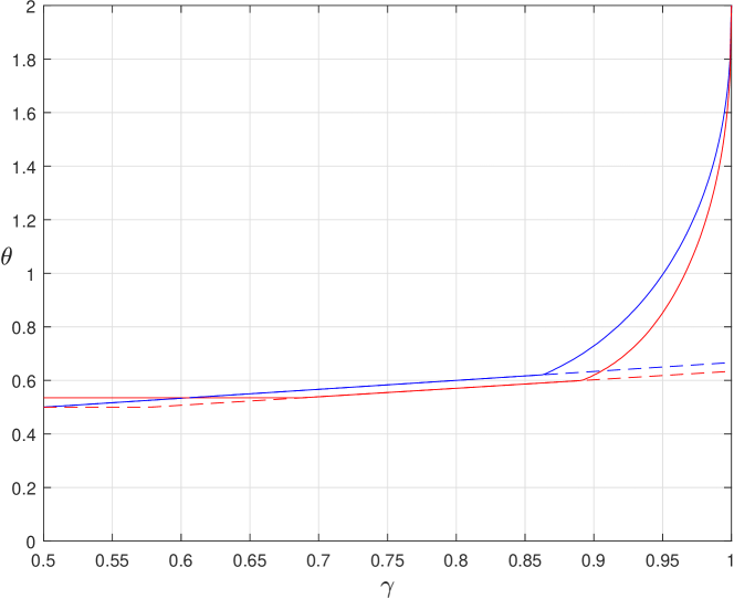
Figure 1: Solid curves: estimated lower stability bounds on $\theta$ versus $\gamma$ in the case of the 2D model advection-diffusion equation with mixed derivative. Dashed curves: analytical lower bounds given by Theorem 4.2 in the case of the 2D model pure diffusion equation with mixed derivative. Red: method (2.3). Blue: method (2.4).

For comparison, the corresponding analytical lower bounds on $\theta$ from Theorem 4.2 for the 2D model pure diffusion problem have been included in the figure as dashed curves. The estimated lower bounds in Figure 1 for the 2D model advection-diffusion problem are close (or equal) to those up to $\gamma\approx 0.89$ and $\gamma\approx 0.86$ for methods (2.3) and (2.4), respectively. Beyond this point, the lower bound for the 2D model advection-diffusion problem increases strongly for both methods, up to $\theta=2$ if $\gamma=1$. In many financial applications, however, $\gamma$ is at most 0.9, and this can be employed in the selection of a (smaller) value $\theta$.

For the stabilizing correction methods (1.7), which use only high-order extrapolation, a similar unconditional stability result in the case of the 2D model pure diffusion equation can be proved as Theorem 4.2 for the two-step modified stabilizing correction methods (1.10). However, in the case of the 2D model advection-diffusion equation (4.15) the stability results for the two-step methods (1.7) appear to be much less favourable than those for the corresponding methods (1.10). Indeed, numerical experiments indicate that for the methods (1.7) given by (2.3) or (2.4) (where $\widecheck{b}$ is now superfluous) unconditional stability is lacking already if $\gamma=0$. In particular, for these methods, considering $z_{0}=0$ and $z_{1}=z_{2}=\textbf{\hskip 1.0pti\hskip 1.0pt}y$ with $y\in\mathbb{R}$, numerical evidence suggests that for each $\theta\geq\frac{1}{2}$ there exists a value $y_{0}\in(0,2)$ such that there is instability whenever $|y|>y_{0}$. A detailed stability study of the two-step methods (1.7) for (4.15) is beyond the scope of this paper, but it appears that at least an upper bound on $q={\mbox{\footnotesize{$\Delta$}}}t/h$ is required to guarantee stability of these methods if advection is present.

We conclude with a brief discussion of the BDF3-type methods (1.7) and (1.10) given by (2.5) when applied to the 2D model equation (4.15). The stability of these three-step methods has been investigated by a numerical study of the pertinent Schur criterion for complex polynomials of degree 3. For method (1.7) given by (2.5), we find that already for the 2D model pure diffusion equation without mixed derivative ($\gamma=0$) unconditional stability is lacking. More precisely, choosing $z_{0}=0$ and $z_{1}=z_{2}=y\in\mathbb{R}$ we find that there is instability whenever $y\lesssim-4.6$, which is clearly a negative result. On the other hand, for method (1.10) given by (2.5), numerical evidence indicates that there is unconditional stability for the 2D model pure diffusion equation if $\gamma\lesssim 0.68$, which is a favourable result. For the general 2D model advection-diffusion equation, an upper bound on $q$ appears to be required however to guarantee stability. For example, taking $z_{0}=0$ and $z_{1}=z_{2}=\textbf{\hskip 1.0pti\hskip 1.0pt}y$ with $y\in\mathbb{R}$, instability is obtained whenever $|y|\gtrsim 2.7$.

5 Test results for the Heston model

To test the methods we consider a test set consisting of six parameter choices for the Heston model. These correspond to those in Haentjens & in ’t Hout [11].

5.1 The Heston model

The Heston model [12] for the fair values of European-style call options leads to a 2D time-dependent PDE of the form

$$\frac{\partial u}{\partial t}=\mbox{\large{$1\over 2$}}s^{2}v\frac{\partial^{2}u}{\partial^{2}s}+\rho\sigma sv\frac{\partial^{2}u}{\partial s\partial v}+\mbox{\large{$1\over 2$}}\sigma^{2}v\frac{\partial^{2}u}{\partial^{2}v}+(r_{\!d}-r_{\!f})s\frac{\partial u}{\partial s}+\kappa(\eta-v)\frac{\partial u}{\partial v}-r_{\!d}\,u$$ (5.1)

with independent variables $t\in(0,T]$ and $s,v>0$, and initial condition

$$u(s,v,0)\,=\,\max(0,s-K)\qquad(s\geq 0,v\geq 0).$$ (5.2)

Here $T>0$ and $K>0$ are the given maturity date and strike price of the option. The parameter $\kappa>0$ is the mean-reversion rate, $\eta>0$ is the long-term mean, $\sigma>0$ is the volatility-of-variance, $\rho\in[-1,1]$ is the correlation between the two underlying Brownian motions, and $r_{d}$, $r_{f}$ denote the domestic and foreign interest rates, respectively. For feasibility of the numerical solution, the spatial domain is truncated to a bounded set $[0,S_{\max}]\times[0,V_{\max}]$ with fixed values $S_{\max}$, $V_{\max}$ taken sufficiently large. The following boundary conditions are imposed, ∂∂u(s,v,t)  =&0  whenever  s=0 ,
∂u∂s(s,v,t)  =e^-r_​ f t  whenever  s=S_max ,
∂u∂su(s,v,t)   =se^-r_​ f t  whenever  v=V_max . Further, at the $v=0$ boundary the PDE (5.1) is fulfilled, see [10].

The spatial discretization of the initial-boundary value problem for (5.1) is performed using second-order finite differences on a smooth, nonuniform, Cartesian grid in the $(s,v)$-domain similar to that in [11, 13]. The spatial grid has relatively many points in the neighbourhood of the location $(s,v)=(K,0)$, which has been done both for financial and numerical reasons. We note that at the boundary $v=0$ the derivative $\partial u/\partial v$ is approximated using a second-order forward finite difference formula. All other derivative terms in the $v$-direction vanish at $v=0$. Cell averaging is applied to define the initial vector obtained from the nonsmooth initial condition (5.2) near the strike, see e.g. [29]. The resulting semi-discrete ODE system (1.1) is splitted according to (1.2) with $s=2$ where $F_{0}$ represents the mixed derivative part and $F_{1}$, respectively $F_{2}$, represents all spatial derivatives in the $s$-direction, respectively $v$-direction, see e.g. [11, 13]. For the subsequent numerical tests we choose the six cases of parameter sets for the Heston model listed in Table 1. These correspond to those from [11].

	Case A	Case B	Case C	Case D	Case E	Case F
$\kappa$	3	0.6067	2.5	0.5	0.3	1
$\eta$	0.12	0.0707	0.06	0.04	0.04	0.09
$\sigma$	0.04	0.2928	0.5	1	0.9	1
$\rho$	0.6	-0.7571	-0.1	-0.9	-0.5	-0.3
$r_{d}$	0.01	0.03	0.0507	0	0	0
$r_{f}$	0.04	0	0.0469	0	0	0
$T$	1	3	0.25	10	15	5
$K$	100	100	100	100	100	100

Table 1: Parameter sets for the Heston model.

Cases A, B, C have previously been considered in [13] and stem from [4, 28, 31], respectively. Here the so-called Feller condition $2\kappa\eta>\sigma^{2}$ always holds. A special feature of Case A is that $\sigma$ is close to zero, which implies that the PDE (5.1) is advection dominated in the $v$-direction. Cases D, E, F were proposed in [1] as challenging test sets for practical applications. In these three cases the maturity times are large and the Feller condition is violated.

5.2 One-step stabilizing correction methods

The multistep methods will be compared with several well-known one-step methods for problems (1.1), (1.2). The Douglas method was already briefly introduced in Section 2. Written out in full, the method reads

$$\left\{\begin{array}[]{ccl}v_{0}&=&u_{n-1}+{\mbox{\footnotesize{$\Delta$}}}t\,F(t_{n-1},u_{n-1})\,,\\[5.69054pt] v_{j}&=&v_{j-1}+\theta{\mbox{\footnotesize{$\Delta$}}}t\big{(}F_{j}(t_{n},v_{j})-F_{j}(t_{n-1},u_{n-1})\big{)}\qquad(j=1,2,\ldots,s)\,,\\[5.69054pt] u_{n}&=&v_{s}\,,\end{array}\right.$$ (5.3)

with parameter $\theta\geq{1\over 2}$. Even if $\theta={1\over 2}$, the order is only one, due to the treatment of the explicit term $F_{0}$ in an Euler fashion. We note that the modification of this method that was recently presented in [2] is not sufficiently stable for the Heston model with explicit treatment of the cross-derivatives.

An extension of the Douglas method, due to in ’t Hout & Welfert [17], is given by

$$\left\{\begin{array}[]{ccl}v^{*}_{0}&=&u_{n-1}+{\mbox{\footnotesize{$\Delta$}}}t\,F(t_{n-1},u_{n-1})\,,\\[5.69054pt] v^{*}_{j}&=&v^{*}_{j-1}+\theta{\mbox{\footnotesize{$\Delta$}}}t\big{(}F_{j}(t_{n},v^{*}_{j})-F_{j}(t_{n-1},u_{n-1})\big{)}\qquad(j=1,2,\ldots,s)\,,\\[5.69054pt] v_{0}&=&v^{*}_{0}+\mbox{\large{$1\over 2$}}{\mbox{\footnotesize{$\Delta$}}}t\big{(}F_{0}(t_{n},v^{*}_{s})-F_{0}(t_{n-1},u_{n-1})\big{)}\\[2.84526pt] &&\;+\,\big{(}\mbox{\large{$1\over 2$}}-\theta\big{)}{\mbox{\footnotesize{$\Delta$}}}t\displaystyle\sum_{j=1}^{s}\big{(}F_{j}(t_{n},v^{*}_{s})-F_{j}(t_{n-1},u_{n-1})\big{)}\,,\\[5.69054pt] v_{j}&=&v_{j-1}+\theta{\mbox{\footnotesize{$\Delta$}}}t\big{(}F_{j}(t_{n},v_{j})-F_{j}(t_{n-1},u_{n-1})\big{)}\qquad(j=1,2,\ldots,s)\,,\\[5.69054pt] u_{n}&=&v_{s}\,.\end{array}\right.$$ (5.4)

If $\theta=\frac{1}{2}$ this is the method of Craig & Sneyd [7]. Taking $\theta\in[\frac{1}{4},\frac{1}{2})$ often gives better accuracy; in the numerical tests we will consider $\theta=\frac{1}{3}$. For any choice of $\theta$, method (5.4) is of order two in the ODE sense. Convergence results for PDEs have been derived in [18]. Stability results for (5.4) applied to the model problems (4.1), (4.15) can be found in [14, 15, 17], for example.

5.3 Results for the Heston model

In the numerical tests we will compare the multistep methods with the following one-step methods:

Do : the Douglas method (5.3) with $\theta=\frac{1}{2}$,

CS : the Craig-Sneyd method, given by (5.4) with $\theta=\frac{1}{2}$,

MCS : the modified Craig-Sneyd method (5.4) with $\theta=\frac{1}{3}$.

Together with these well-known one-step methods we consider the following two-step methods (1.10) with modified stabilizing corrections:

SC2A : the Adams2-type method (2.4) with $\theta=\frac{3}{4}$,

SC2B : the BDF2-type method (2.3) with $\theta=\frac{2}{3}$,

SC2C : the CNLF-type method (2.2) with $\theta=1$.

In these Adams2- and BDF2-type methods the parameter value $\theta$ was chosen so as to give a reasonable compromise between stability properties and error constants. The same holds for the modified Craig-Sneyd method.

Figure 2: Global errors at $t=T$ versus $1/N$ for the test cases A–F. Methods CS and MCS with step-size ${\mbox{\footnotesize{$\Delta$}}}t=T/N$, Douglas method and the multistep methods with step-size ${\mbox{\footnotesize{$\Delta$}}}t=T/[2N]$.

Per step, the methods CS and MCS are twice as expensive as the others, and therefore we will use these methods with a step-size two times larger than for the Douglas method and the multistep methods. For the two-step methods, the first approximation $u_{1}$ was computed with the Douglas method with $\theta=1$, which seems a natural starting method for the stabilizing correction two-step methods.

In Figure 2 the results are found for the six cases of Heston parameter sets given by Table 1. In these plots, the global errors in the maximum norm are plotted as a function of $1/N$, where $T/N$ is the step-size used for the CS and MCS methods. Here a $400\times 200$ spatial grid has been taken and the global error is considered for $t=T$ on a region of financial interest given by $\frac{1}{2}K<s<\frac{3}{2}K$ and $0<v<1$. Note that the global error does not contain the error due to spatial discretization.

From Figure 2 it is seen that the two-step methods with stabilizing corrections based on the implicit Adams method (SC2A) and implicit BDF2 method (SC2B) are competitive with the modified Craig-Sneyd method (MCS).

The CNLF method (SC2C) behaves quite poorly in all six cases, with large errors for moderate step-sizes and an irregular error behaviour, probably due to instability. Indeed, in Section 4 it was noticed that for the 2D model advection-diffusion problem already a small amount of advection can render this method unstable.

Remark 5.1 (Smoothing steps).

The accuracy of the one-step methods in these tests can be somewhat improved by performing two (non-splitted) backward Euler sub-steps with step-size $\frac{1}{2}{\mbox{\footnotesize{$\Delta$}}}t$ to compute the first approximation $u_{1}\approx u({\mbox{\footnotesize{$\Delta$}}}t)$. These are the so-called Rannacher smoothing steps [25]. The positive effect was most pronounced for the methods Do and CS, but even with such smoothing steps these two methods are not competitive with the best methods in these tests (MCS, SC2A and SC2B). For a simple comparison of the methods, with comparable work for all methods, such (non-splitted) backward Euler smoothing steps were not used in the tests. Moreover, at the moment, it is not clear how a proper smoothing procedure should be constructed for the multistep methods. $\Diamond$

Remark 5.2 (Two-step methods (1.7)).

The lower order extrapolation in (1.10) was introduced to improve stability of the schemes. In the above tests this enhanced stability was found to be necessary, in particular for the Adams2-type scheme. The BDF2-type method showed a more stable behaviour but also that method failed for the advection dominated PDE given by Case A.

For step-sizes that are sufficiently small for having stability, say ${\mbox{\footnotesize{$\Delta$}}}t\leq\tau_{\rm stab}$, the accuracy of these two-step methods (1.7) was in general slightly better than for the corresponding methods (1.10). However, the stability threshold $\tau_{\rm stab}$ depends on the problem and on the spatial mesh-width.

Since robustness is an important quality in option valuation applications, the modified methods (1.10) are, in our opinion, preferable over the schemes (1.7). $\Diamond$

Remark 5.3 (Three-step methods (1.10)).

Tests were also performed with the stabilizing corrections BDF3-type scheme (1.10) with coefficients (2.5). Starting values $u_{1}$ and $u_{2}$ were computed with the MCS method. For smaller step-sizes this SC3B method was seen to give higher accuracy than the two-step methods SC2A and SC2B, but instabilities were again observed for larger step-sizes, making this method not suitable for the Heston problem. (Needless to say, the BDF3-type scheme (1.7) with high-order extrapolation turned out to be very unstable.) $\Diamond$

6 Concluding remarks

Among the two-step methods with stabilizing corrections (1.10) considered in this paper the behaviour of the methods based on BDF2 and Adams2 was satisfactory, and these methods appear to be competitive with the well-established modified Craig-Sneyd method for the Heston problem. The BDF3-type scheme (1.10) may be suited for other applications, such as reaction-diffusion problems, which is left for future research.

The stabilizing correction methods studied in this paper can be viewed as generalizations of IMEX linear multistep methods. Such IMEX multistep methods have been examined for 1D option valuation models with jumps in [26]. Based on accuracy, the authors had a slight preference for the CNAB method, i.e. (2.4) with $\theta=\frac{1}{2}$, over the BDF2 method. Subsequently, this CNAB method was applied to 2D models in [27], but without dimension splitting. It is part of our research plans to examine the behaviour of the stabilizing correction multistep schemes to models with jumps together with dimension splitting.

References

• [1] L. Andersen, Simple and efficient simulation of the Heston stochastic volatility model. J. Comp. Finan. 11 (2008), 1–42.
• [2] A. Arrarás, K.J. in ’t Hout, W. Hundsdorfer, L. Portero, Modified Douglas splitting methods for reaction-diffusion equations. BIT Numer. Math. 57 (2017), 261–285.
• [3] U.M. Ascher, S.J. Ruuth, B.T.R. Wetton, Implicit-explicit methods for time-dependent partial differential equations. SIAM J. Numer. Anal. 32 (1995), 797–823.
• [4] Bloomberg Quant. Finan. Devel. Group, Barrier options pricing under the Heston model, 2005.
• [5] O.P. Bruno, M. Cubillos, Higher-order in time “quasi-unconditionally stable” ADI solvers for the compressible Navier-Stokes equations in 2D and 3D curvilinear domains. J. Comp. Phys. 307 (2016), 476–495.
• [6] M. Crouzeix, Une méthode multipas implicite-explicite pour l’approximation des équations d’évolution paraboliques. Numer. Math. 35 (1980), 257–276.
• [7] I.J.D. Craig, A.D. Sneyd, An alternating-direction implicit scheme for parabolic equations with mixed derivatives. Comput. Math. Appl. 16 (1988), 341–350.
• [8] J. Douglas, Alternating direction methods for three space variables. Numer. Math. 4 (1962), 41–63.
• [9] J. Douglas, J.E. Gunn, A general formulation of alternating direction methods. Numer. Math. 6 (1964), 428–453.
• [10] E. Ekström, J. Tysk, The Black-Scholes equation in stochastic volatility models. J. Math. Anal. Appl. 368 (2010), 498–507.
• [11] T. Haentjens, K.J. in ’t  Hout, Alternating direction implicit finite difference schemes for the Heston-Hull-White partial differential equation. J. Comp. Finan. 16 (2012), 83–110.
• [12] S.L. Heston, A closed-form solution for options with stochastic volatility with applications to bond and currency options. Rev. Finan. Stud. 6 (1993), 327–343.
• [13] K.J. in ’t  Hout, S. Foulon, ADI finite difference schemes for option pricing in the Heston model with correlation. Int. J. Numer. Anal. Mod. 7 (2010), 303–320.
• [14] K.J. in ’t  Hout, C. Mishra, Stability of the modified Craig-Sneyd scheme for two-dimensional convection-diffusion equations with mixed derivative term. Math. Comp. Simul. 81 (2011), 2540–2548.
• [15] K.J. in ’t  Hout, C. Mishra, Stability of ADI schemes for multidimensional diffusion equations with mixed derivative terms. Appl. Numer. Math. 74 (2013), 83–94.
• [16] K.J. in ’t  Hout, B.D. Welfert, Stability of ADI schemes applied to convection-diffusion equations with mixed derivative terms. Appl. Numer. Math. 57 (2007), 19–35.
• [17] K.J. in ’t  Hout, B.D. Welfert, Unconditional stability of second-order ADI schemes applied to multi-dimensional diffusion equations with mixed derivative terms. Appl. Numer. Math. 59 (2009), 677–692.
• [18] K.J. in ’t  Hout, M. Wyns, Convergence of the Modified Craig-Sneyd scheme for two-dimensional convection-diffusion equations with mixed derivative term. J. Comp. Appl. Math. 296 (2016), 170–180.
• [19] W. Hundsdorfer, Partially implicit BDF2 blends for convection dominated flows. SIAM J. Numer. Anal. 38 (2001), 1763–1783.
• [20] W. Hundsdorfer, Accuracy and stability of splitting with stabilizing corrections. Appl. Numer. Math. 42 (2002), 213–233.
• [21] W. Hundsdorfer, J.G. Verwer, Numerical Solution of Time-Dependent Advection-Diffusion-Reaction Equations. Springer, 2003.
• [22] G.I. Marchuk, Splitting and alternating direction methods. In: Handbook of Numerical Analysis I. Eds. P.G. Ciarlet, J.L. Lions, North-Holland, 1990, 197–462.
• [23] S. McKee, A.R. Mitchell, Alternating direction methods for parabolic equations in two space dimensions with a mixed derivative. Comput. J. 13 (1970), 81–86.
• [24] O. Nevanlinna, W. Liniger, Contractive methods for stiff differential equations, II. BIT 19 (1979), 53–72.
• [25] R. Rannacher, Finite element solution of diffusion problems with irregular data. Numer. Math. 43 (1984), 309–327.
• [26] S. Salmi, J. Toivanen, IMEX schemes for pricing options under jump-diffusion models. Appl. Numer. Math. 84 (2014), 33–45.
• [27] S. Salmi, J. Toivanen, L. von Sydow, An IMEX-scheme for pricing options under stochastic volatility models with jumps. SIAM J. Sci. Comp. 36 (2014), B817–B834.
• [28] W. Schoutens, E. Simons, J. Tistaert, A perfect calibration! Now what?. Wilmott mag., March 2004, 66–78.
• [29] D. Tavella, C. Randall, Pricing Financial Instruments: The Finite Difference Method. John Wiley & Sons, 2000.
• [30] J.M. Varah, Stability restrictions on second order, three level finite difference schemes for parabolic equations. SIAM J. Numer. Anal. 17 (1980), 300–309.
• [31] G. Winkler, T. Apel, U. Wystup, Valuation of options in Heston’s stochastic volatility model using finite element methods. In: Foreign Exchange Risk. Eds. J. Hakala, U. Wystup, Risk Books, 2002, 283–303.