The Convex Feasible Set Algorithm
for Real Time Optimization in Motion Planning

Abstract

With the development of robotics, there are growing needs for real time motion planning. However, due to obstacles in the environment, the planning problem is highly non-convex, which makes it difficult to achieve real time computation using existing non-convex optimization algorithms. This paper introduces the convex feasible set algorithm (CFS) which is a fast algorithm for non-convex optimization problems that have convex costs and non-convex constraints. The idea is to find a convex feasible set for the original problem and iteratively solve a sequence of subproblems using the convex constraints. The feasibility and the convergence of the proposed algorithm are proved in the paper. The application of this method on motion planning for mobile robots is discussed. The simulations demonstrate the effectiveness of the proposed algorithm.

90C55, 90C26, 68T40, 93C85

1 Introduction

Although great progresses have been made in robot motion planning [15], the field is still open for research regarding real time planning in dynamic uncertain environment. The applications include but are not limited to real time navigation [10], autonomous driving [14, 18], robot arm manipulation and human robot cooperation [17]. To achieve safety and efficiency, robot motion should be re-planned from time to time when new information is obtained during operation. The motion planning algorithm should run fast enough to meet the real time requirement for planning and re-planning.

In this paper, we focus on optimization-based motion planning methods, which fit into the framework of model-predictive control (MPC) [12], where the optimal trajectory is obtained by solving a constrained optimization at each time step. As there are obstacles in the environment, the constraints are highly non-convex, which makes the problem hard to solve in real time. Various methods have been developed to deal with the non-convexity [23, 28]. One popular way is through convexification [29], e.g., transforming the non-convex problem into a convex one. Some authors propose to transform the non-convex problem to semidefinite programming (SDP) [8]. Some authors introduce lossless convexification by augmenting the space [3, 11]. And some authors use successive linear approximation to remove non-convex constraints [20, 21]. However, the first method can only handle quadratic cost functions. The second approach highly depends on the linearity of the system and may not be able to handle diverse obstacles. The third approach may not generalize to non-differentiable problems. Another widely-used convexification method is the sequential quadratic programming (SQP) [27, 30], which approximates the non-convex problem as a sequence of quadratic programming (QP) problems and solves them iteratively. The method has been successfully applied to offline robot motion planning [13, 26]. However, as SQP is a generic algorithm, the unique geometric structure of the motion planning problems is neglected, which usually results in failure to meet the real time requirement in engineering applications.

Typically, in a motion planning problem, the constraints are physically determined, while the objective function is designed to be convex [31, 24]. The non-convexity mainly comes from the physical constraints. Regarding this observation, a fast algorithm called the convex feasible set algorithm (CFS) is proposed in this paper to solve optimization-based motion planning problems with convex objective functions and non-convex constraints.

The main idea of the CFS algorithm is to transform the original problem into a sequence of convex subproblems by obtaining convex feasible sets within the non-convex domain, then iteratively solve the convex subproblems until convergence. The idea is similar to SQP in that it tries to solve several convex subproblems iteratively. The difference between CFS and SQP lies in the way to obtain the convex subproblems. The geometric structure of the original problem is fully considered in CFS. This strategy will make the computation faster than conventional SQP and other non-convex optimization methods such as interior point (ITP) [32], as will be demonstrated later. Moreover, local optima is guaranteed.

It is worth noting that the convex feasible set in the trajectory space can be regarded as a convex corridor. The idea of using convex corridors to simplify the motion planning problems has been discussed in [5, 33]. However, these methods are application-specific without theoretical guarantees. In this paper, we consider general non-convex and non-differentiable optimization problems (which may not only arise from motion planning problems, but also other problems) and provide theoretical guarantees of the method.

The remainder of the paper is organized as follows. Section 2 proposes a benchmark optimization problem. Section 3 discusses the proposed CFS algorithm in solving the benchmark problem. Section 4 shows the feasibility and convergence of the algorithm. Section 5 illustrates the application of the algorithm on motion planning problems for mobile robots. Section 6 concludes the paper.

2 The Optimization Problem

2.1 The Benchmark Problem

Consider an optimization problem with a convex cost function but non-convex constraints, i.e.,

(1) $$\min_{\mathbf{x}\in\Gamma}J(\mathbf{x}),$$

where $\mathbf{x}\in\mathbb{R}^{n}$ is the decision variable and the problem follows two assumptions. [Cost] $J:\mathbb{R}^{n}\rightarrow\mathbb{R}^{+}$ is smooth and strictly convex. [Constraint] The set $\Gamma\subset\mathbb{R}^{n}$ is connected and closed, with piecewise smooth and non-self-intersecting boundary $\partial\Gamma$. For every point $x\in\Gamma$, there exists an $n$-dimensional convex polytope $P\subset\Gamma$ such that $x\in P$.

Eq. 1 implies that $J$ is radially unbounded, i.e., $J(\mathbf{x})\rightarrow\infty$ when $\|\mathbf{x}\|\rightarrow\infty$. Eq. 1 specifies the geometric features of the feasible set $\Gamma$, where the first part deals with the topological features of $\Gamma$ and the second part ensures that there is a convex neighborhood for any point in $\Gamma$. Note that equality constraints in $\Gamma$ are excluded by Eq. 1 as the dimension of the neighborhood for any point satisfying a equality constraint is strictly less than $n$.

The geometric structure of problem Eq. 1 is illustrated in Fig. 1a. The contour represents the cost function $J$, while the gray parts represent $\Gamma^{c}$. There are two disjoint components in $\Gamma^{c}$. The goal is to find a local optimum (hopefully global optimum) starting from the initial reference point (blue dot). As shown in Fig. 1a, the problem is highly non-convex and the non-convexity comes from the constraints. To make the computation efficient, we propose the convex feasible set algorithm in this paper, which transforms problem Eq. 1 into a sequence of convex optimizations by obtaining a sequence of convex feasible sets inside the non-convex domain $\Gamma$. As shown in Fig. 1, the idea is implemented iteratively. At current iteration, a convex feasible set for the current reference point (blue dot) is obtained. The optimal solution in the convex feasible set (black dot) is set as the reference point for the next iteration. The formal mathematical description of this algorithm will be discussed in Section 3. The feasibility of this method, i.e., the existence of an $n$-dimensional convex feasible set, is implied by Eq. 1. Nonetheless, in order to compute the convex feasible set efficiently, we still need an analytical description of the constraint, which will be discussed in Section 2.2.

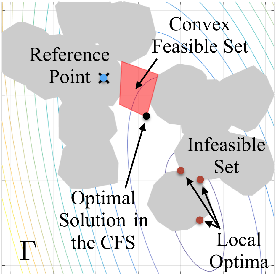
(a) Iteration 1.

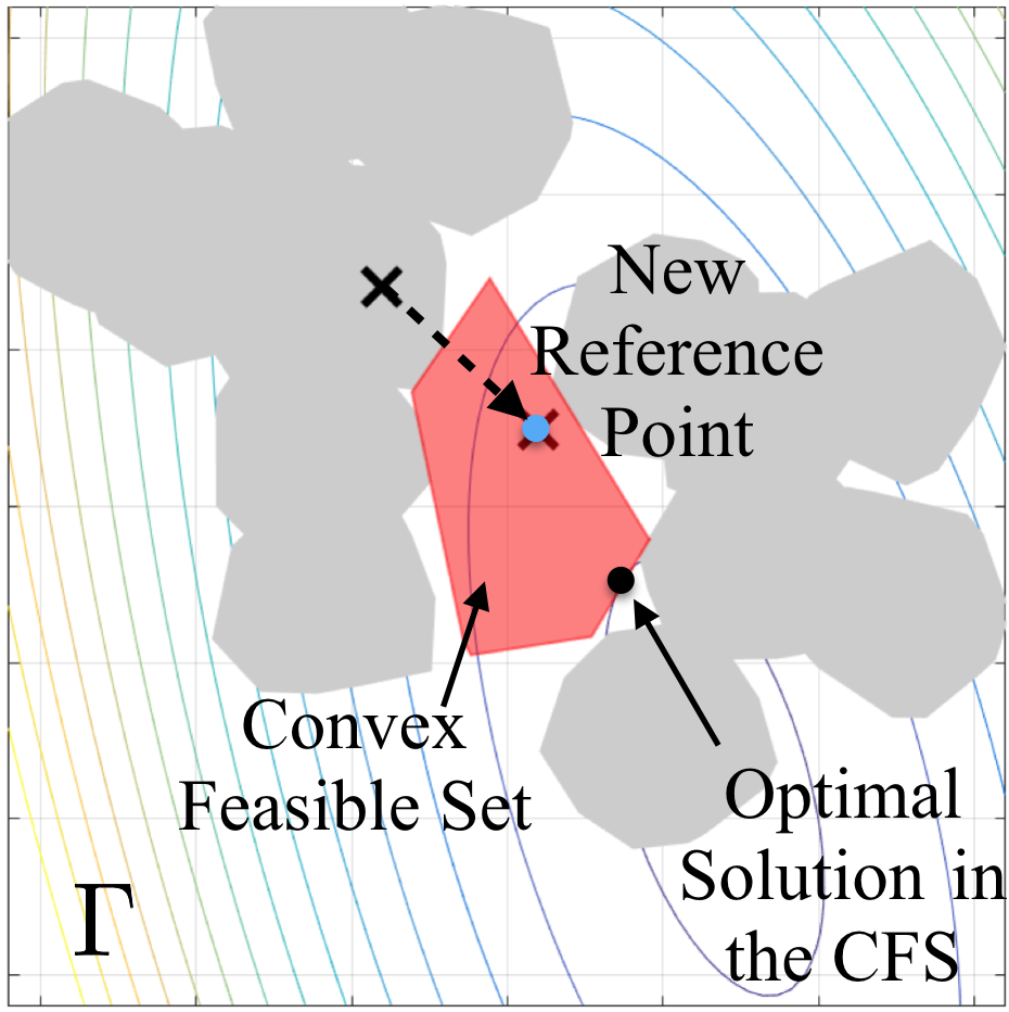
(b) Iteration 2.

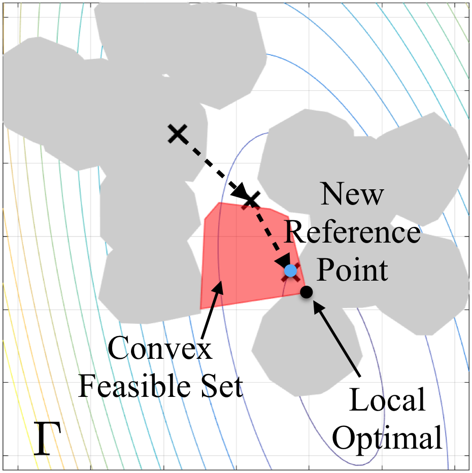
(c) Iteration 3.

Figure 1: Geometry of problem Eq. 1 and the idea of the convex feasible set algorithm.

2.2 Analytical Representation of the Constraints

The set $\Gamma$ will be represented analytically by several inequality constraints. It is called a semi-convex decomposition of $\Gamma$ if

(2) $$\Gamma=\bigcap_{i=1}^{N}\{\mathbf{x}:\phi_{i}(\mathbf{x})\geq 0\}=\bigcap_{i=1}^{N}\Gamma_{i},$$

for $N$ continuous, piecewise smooth and semi-convex functions $\phi_{i}:\mathbb{R}^{n}\rightarrow\mathbb{R}$ such that $\Gamma_{i}:=\{\mathbf{x}:\phi_{i}(\mathbf{x})\geq 0\}$ with $\partial\Gamma_{i}=\{\mathbf{x}:\phi_{i}(\mathbf{x})=0\}$. Semi-convexity [7] of $\phi_{i}$ implies that there exists a positive semi-definite $H_{i}^{*}\in\mathbb{R}^{n\times n}$ such that the function

(3) $$\tilde{\phi}_{i}(\mathbf{x}):=\phi_{i}(\mathbf{x})+\frac{1}{2}(\mathbf{x}-\mathbf{x}_{0})^{T}H_{i}^{*}(\mathbf{x}-\mathbf{x}_{0}),$$

is convex in $\mathbf{x}$ for any $\mathbf{x}_{0}\in\mathbb{R}^{n}$. Or in other words, the hessian of $\phi_{i}$ is bounded below. Note that $\Gamma_{i}^{c}$’s are not required to be disjoint and $N$ should be greater than or equal to the number of disjoint components in $\Gamma^{c}$. The decomposition from $\Gamma$ to $\Gamma_{i}$’s is not unique. Neither is the function $\phi_{i}$ that represents $\Gamma_{i}$. In many cases, $\phi_{i}$ can be chosen as a signed distance function to $\partial\Gamma_{i}$, which will be discussed in Section 5.2.

Before introducing more conditions on the decomposition Eq. 2, analytical properties of the functions $\phi_{i}$’s will be studied first. Since $\tilde{\phi}_{i}$ is convex, then for any $\mathbf{x}_{0},v\in\mathbb{R}^{n}$, $\tilde{\phi}_{i}(\mathbf{x}_{0}+v)-2\tilde{\phi}_{i}(\mathbf{x}_{0})+\tilde{\phi}_{i}(\mathbf{x}_{0}-v)\geq 0$. Consider Eq. 3, the following inequality holds for any semi-convex functions,

(4) $$\phi_{i}(\mathbf{x}_{0}+v)-2\phi_{i}(\mathbf{x}_{0})+\phi_{i}(\mathbf{x}_{0}-v)\geq-v^{T}H_{i}^{*}v.$$

Moreover, since convex functions are locally Lipschitz [2], $\phi_{i}$ is also locally Lipschitz as implied by definition Eq. 3. However, as $\phi_{i}$ is only piecewise smooth, it may not be differentiable everywhere. For any $v\in\mathbb{R}^{n}$, define the one-side directional derivative $\partial_{v}$ as

(5) $$\partial_{v}\phi_{i}(\mathbf{x}):=\lim_{a\rightarrow 0^{+}}\frac{\phi_{i}(\mathbf{x}+av)-\phi_{i}(\mathbf{x})}{a}.$$

For any $\|v\|=1$, $\partial_{v}\phi_{i}(\mathbf{x})$ is bounded locally since $\phi_{i}$ is locally Lipschitz. If $\phi_{i}$ is smooth at direction $v$ at point $\mathbf{x}$, then

(6) $$\lim_{a\rightarrow 0^{+}}\frac{\phi_{i}(\mathbf{x}+av)-\phi_{i}(\mathbf{x})}{a}=\lim_{a\rightarrow 0^{-}}\frac{\phi_{i}(\mathbf{x}+av)-\phi_{i}(\mathbf{x})}{a}=\lim_{a\rightarrow 0^{+}}\frac{\phi_{i}(\mathbf{x}-av)-\phi_{i}(\mathbf{x})}{-a},$$

where the second equality is by taking negative of $a$. By definition Eq. 5, the right-hand side of Eq. 6 equals to $-\partial_{-v}\phi_{i}(\mathbf{x})$, which implies that $\partial_{v}\phi_{i}(\mathbf{x})=-\partial_{-v}\phi_{i}(\mathbf{x})$. Let $\mathcal{S}(\phi_{i},\mathbf{x}):=\{v\in\mathbb{R}^{n}:\partial_{v}\phi_{i}(\mathbf{x})+\partial_{-v}\phi_{i}(\mathbf{x})=0\}$ denote all the smooth directions of function $\phi_{i}$ at point $\mathbf{x}$. The directional derivatives satisfy the following properties.

Lemma 2.1 (Properties of Directional Derivatives).

If $\phi_{i}$ is continuous, piecewise smooth, and semi-convex, then for any $\mathbf{x},v,v_{1},v_{2}\in\mathbb{R}^{n}$ and $b\in\mathbb{R}$ such that $v=v_{1}+v_{2}$, the following inequalities hold,

(7) $$0 \leq\partial_{v}\phi_{i}(\mathbf{x})+\partial_{-v}\phi_{i}(\mathbf{x}),$$

(8) $$b\partial_{v}\phi_{i}(\mathbf{x}) \leq\partial_{bv}\phi_{i}(\mathbf{x}),$$

(9) $$\partial_{v}\phi_{i}(\mathbf{x}) \leq\partial_{v_{1}}\phi_{i}(\mathbf{x})+\partial_{v_{2}}\phi_{i}(\mathbf{x}).$$

The equalities in Eq. 7 and Eq. 8 are achieved when $v\in\mathcal{S}(\phi_{i},\mathbf{x})$. The equality in Eq. 9 is achieved when $v_{1},v_{2}\in\mathcal{S}(\phi_{i},\mathbf{x})$.

Proof 2.2.

If $\phi_{i}$ is semi-convex, Eq. 4 implies that for any scalar $a$ and vector $v$,

$$\frac{\phi_{i}(\mathbf{x}+av)-2\phi_{i}(\mathbf{x})+\phi_{i}(\mathbf{x}-av)}{a}\geq-av^{T}H_{i}^{*}v.$$

Let $a\rightarrow 0^{+}$. The left-hand side approaches $\partial_{v}\phi_{i}(\mathbf{x})+\partial_{-v}\phi_{i}(\mathbf{x})$, while the right-hand side approaches $0$ in the limits. Hence Eq. 7 holds. By definition Eq. 5, $\partial_{bv}\phi_{i}(\mathbf{x})=b\partial_{v}\phi_{i}(\mathbf{x})$ when $b\geq 0$. When $b<0$, by Eq. 7, $-|b|\partial_{v}\phi_{i}(\mathbf{x})\leq|b|\partial_{-v}\phi_{i}(\mathbf{x})=\partial_{-|b|v}\phi_{i}(\mathbf{x})=\partial_{bv}\phi_{i}(\mathbf{x})$. Hence Eq. 8 holds. The equality holds when $\partial_{v}\phi_{i}(\mathbf{x})+\partial_{-v}\phi_{i}(\mathbf{x})=0$, i.e., $v\in\mathcal{S}(\phi_{i},\mathbf{x})$. Moreover, Eq. 4 also implies

$$-\frac{a^{2}}{4}(v_{1}-v_{2})^{T}H_{i}^{*}(v_{1}-v_{2})\leq\phi_{i}(\mathbf{x}+av_{1})-2\phi_{i}(\mathbf{x}+a\frac{v}{2})+\phi_{i}(\mathbf{x}+av_{2})$$

$$=\phi_{i}(\mathbf{x}+av_{1})-\phi_{i}(\mathbf{x})+\phi_{i}(\mathbf{x}+av_{2})-\phi_{i}(\mathbf{x})-2[\phi_{i}(\mathbf{x}+a\frac{v}{2})-\phi_{i}(\mathbf{x})].$$

Divide the both sides by $a$ and take $a\rightarrow 0^{+}$. Then the left-hand side approaches $0$, while the right-hand side approaches $\partial_{v_{1}}\phi_{i}(\mathbf{x})+\partial_{v_{2}}\phi_{i}(\mathbf{x})-\partial_{v}\phi_{i}(\mathbf{x})$. Hence Eq. 9 holds. When $v_{1},v_{2}\in\mathcal{S}(\phi_{i},\mathbf{x})$,

(10) $$0\leq\partial_{v}\phi_{i}(\mathbf{x})+\partial_{-v}\phi_{i}(\mathbf{x})\leq\partial_{v_{1}}\phi_{i}(\mathbf{x})+\partial_{v_{2}}\phi_{i}(\mathbf{x})+\partial_{-v_{1}}\phi_{i}(\mathbf{x})+\partial_{-v_{2}}\phi_{i}(\mathbf{x})=0.$$

The first inequality is due to Eq. 7; the second inequality is due to Eq. 9. Hence the equality in Eq. 9 is attained.

Define the sub-differential of $\phi_{i}$ at $\mathbf{x}$ as

(11) $$D\phi_{i}(\mathbf{x}):=\{d\in\mathbb{R}^{n}:d\cdot v\leq\partial_{v}\phi_{i}(\mathbf{x}),\forall v\in\mathbb{R}^{n}\}.$$

The validity of the definition, i.e., the right-hand side of Eq. 11 is non empty, can be verified by Lemma 2.1. By Eq. 8 and Eq. 9, for any $v_{1},v_{2}\in\mathcal{S}(\phi_{i},\mathbf{x})$, $a,b\in\mathbb{R}$ and $v=av_{1}+bv_{2}$, we have $\partial_{v}\phi_{i}(\mathbf{x})=a\partial_{v_{1}}\phi_{i}(\mathbf{x})+b\partial_{v_{2}}\phi_{i}(\mathbf{x})$ and $\partial_{v}\phi_{i}(\mathbf{x})+\partial_{-v}\phi_{i}(\mathbf{x})=0$. Hence $v\in\mathcal{S}(\phi_{i},\mathbf{x})$. We can conclude that 1) $\mathcal{S}(\phi_{i},\mathbf{x})$ is a linear subspace of $\mathbb{R}^{n}$ and 2) the function induced by the directional derivative $v\mapsto\partial_{v}\phi_{i}(\mathbf{x})$ is a sub-linear function on $\mathbb{R}^{n}$ and a linear function on $\mathcal{S}(\phi_{i},\mathbf{x})$. By Hahn-Banach Theorem [9], there exists a vector $d\in\mathbb{R}^{n}$ such that $d\cdot v=\partial_{v}\phi_{i}(\mathbf{x})$ for $v\in\mathcal{S}(\phi_{i},\mathbf{x})$ and $d\cdot v\leq\partial_{v}\phi_{i}(\mathbf{x})$ for $v\in\mathbb{R}^{n}$. Moreover, as the unit directional derivative is bounded, the sub-gradients are also bounded. Hence the definition in Eq. 11 is justified. The elements in $D\phi_{i}(\mathbf{x})$ are called sub-gradients. When $\phi_{i}$ is smooth at $\mathbf{x}$, $D\phi_{i}(\mathbf{x})$ reduces to a singleton set which contains only the gradient $\nabla\phi_{i}(\mathbf{x})$ such that $\nabla\phi_{i}(\mathbf{x})\cdot v=\partial_{v}\phi_{i}(\mathbf{x})$ for all $v\in\mathbb{R}^{n}$. The definition Eq. 11 follows from Clarke (generalized) sub-gradients for non-convex functions [6].

With the definition of sub-differential for continuous, piecewise smooth and semi-convex functions in Eq. 11, the following assumption regarding the analytical representation is made. [Analytical Representations] For $\Gamma$ satisfying Eq. 1, there exists a semi-convex decomposition Eq. 2 such that 1) $D\phi_{i}(\mathbf{x})\neq\{0\}$ for all $\mathbf{x}$, 2) $0\notin D\phi_{i}(\mathbf{x})$ if $\mathbf{x}\in\partial\Gamma_{i}$, and 3) for any $\mathbf{x}$ such that $I:=\{i:\phi_{i}(\mathbf{x})=0\}\neq\emptyset$, there exists $v\in\mathbb{R}^{n}$ such that $\partial_{v}\phi_{i}(\mathbf{x})<0$ for all $i\in I$.

Note that the hypothesis that any $\Gamma$ that satisfies Eq. 1 has a semi-convex decomposition that satisfies 2.2 will be verified in our future work. A method to construct the desired $\phi_{i}$’s is discussed in [16].

The first condition in 2.2 ensures that $\phi_{i}$ will not have smooth extreme points. Geometrically, the second condition in 2.2 implies that there cannot be any concave corners in $\Gamma_{i}^{c}$ or convex corners in $\Gamma_{i}$. Suppose $\Gamma_{i}^{c}$ has a concave corner at $\mathbf{x}\in\partial\Gamma_{i}$. Since $0\notin D\phi_{i}(\mathbf{x})$, we can choose a unit vector $v$ such that $\partial_{v}\phi_{i}(\mathbf{x})<0$ and $\partial_{-v}\phi_{i}(\mathbf{x})<0$ as shown in Fig. 2a. Then Eq. 7 is violated, which contradicts with the assumption on semi-convexity. Nonetheless, concave corners are allowed in $\Gamma^{c}$, but should only be formulated by a union of several intersecting $\Gamma_{i}^{c}$’s as shown in Fig. 2b. In the example, the set $\Gamma=\{\mathbf{x}=(x_{1},x_{2}):\min(|x_{1}|-1,|x_{2}|-1)\geq 0\}$ is partitioned into two sets $\Gamma_{1}=\{\mathbf{x}:|x_{1}|-1\geq 0\}$ and $\Gamma_{2}=\{\mathbf{x}:|x_{2}|-1\geq 0\}$. Both $\phi_{1}=|x_{1}|-1$ and $\phi_{2}=|x_{1}|-1$ satisfy 2.2. Without the partition, $\phi=\min(|x_{1}|-1,|x_{2}|-1)$ violates the condition on semi-convexity. The third condition in 2.2 implies that once $\Gamma_{i}^{c}$’s intersect, they should have common interior among one another. For example, the decomposition in Fig. 2c is not allowed. In this case, the obstacle is partitioned into five components. $\partial\Gamma_{2}^{c}$, $\partial\Gamma_{3}^{c}$, and $\partial\Gamma_{5}^{c}$ intersect at $\mathbf{x}$. However, there does not exist $v\in\mathbb{R}^{n}$ such that $\partial_{v}\phi_{i}(\mathbf{x})<0$ for all $i\in\{2,3,5\}$ as the interiors of $\Gamma_{2}^{c}$ and $\Gamma_{3}^{c}$ do not intersect. This condition is enforced in order to ensure that the computed convex feasible set is non empty as will be discussed in Lemma 4.2.

In this following discussion, $\phi_{i}$’s and $\Gamma_{i}$’s are referred as the semi-convex decomposition of $\Gamma$ that satisfies 2.2.

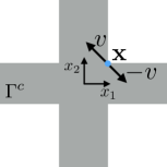
(a) The constraint $\Gamma$.

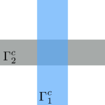
(b) Valid decomposition of $\Gamma$.

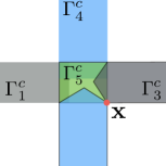
(c) Invalid decomposition of $\Gamma$.

Figure 2: Representing $\Gamma$ using $\Gamma_{i}$ and $\phi_{i}$.

2.3 Physical Interpretations

Many motion planning problems can be formulated into Eq. 1 when $\mathbf{x}$ is regarded as the trajectory as will be discussed in Section 5. The dimension of the problem $n$ is proportional to the number of sampling points on the trajectory. If continuous trajectories are considered, then $n\rightarrow\infty$ and $\mathbb{R}^{n}$ approaches the space of continuous functions $\mathcal{C}(\mathbb{R})$ in the limit.

In addition to motion planning problems, the proposed method deals with any problem with similar geometric properties as specified in Eq. 1 and Eq. 1. Moreover, problems with global linear equality constraints also fit into the framework if we solve the problem in the low-dimensional linear manifold defined by the linear equality constraints. The case for nonlinear equality constraints is much trickier since convexification on nonlinear manifold is difficult in general. A relaxation method to deal with nonlinear equality constraints is discussed in [19].

3 Solving the Optimization Problem

3.1 The Convex Feasible Set Algorithm

To solve the problem Eq. 1 efficiently, we propose the convex feasible set algorithm. As introduced in Section 2.1, a convex feasible set $\mathcal{F}$ for the set $\Gamma$ is a convex set such that $\mathcal{F}\subset\Gamma$. $\mathcal{F}$ is not unique. We define the desired $\mathcal{F}$ in Section 3.2. As $\Gamma$ can be covered by several (may be infinitely many) convex feasible sets, we can efficiently search the non-convex space $\Gamma$ for solutions by solving a sequence of convex optimizations constrained in a sequence of convex feasible sets. The idea is implemented iteratively as shown in Fig. 1. At iteration $k$, given a reference point $\mathbf{x}^{(k)}$, a convex feasible set $\mathcal{F}^{(k)}:=\mathcal{F}(\mathbf{x}^{(k)})\subset\Gamma$ is computed around $\mathbf{x}^{(k)}$. Then a new reference point $\mathbf{x}^{(k+1)}$ will be obtained by solving the resulting convex optimization problem

(12) $$\mathbf{x}^{(k+1)}=\arg\min_{\mathbf{x}\in\mathcal{F}^{(k)}}J(\mathbf{x}).$$

The optimal solution will be used as the reference point for the next step. The iteration will terminate if either the change in solution is small, e.g.,

(13) $$\|\mathbf{x}^{(k+1)}-\mathbf{x}^{(k)}\|\leq\epsilon_{1},$$

for some small $\epsilon_{1}>0$, or the descent in cost is small, e.g.,

(14) $$J(\mathbf{x}^{(k)})-J(\mathbf{x}^{(k+1)})\leq\epsilon_{2},$$

for some small $\epsilon_{2}>0$. We will show in Section 4 that these two conditions are equivalent and both of them imply convergence. The process is summarized in Algorithm 1.

Algorithm 1 The Convex Feasible Set Algorithm

  Initialize initial guess $\mathbf{x}^{(0)}$, $k:=0$;

  while True do

     Find a convex feasible set $\mathcal{F}^{(k)}\subset\Gamma$ for $\mathbf{x}^{(k)}$;

     Solve the convex optimization problem Eq. 12 for $\mathbf{x}^{(k+1)}$;

     if Eq. 13 or Eq. 14 is satisfied then

        Break the while loop;

     end if

     $k:=k+1$;

  end while

  return  $\mathbf{x}^{(k+1)}$;

3.2 Finding the Convex Feasible Set

Considering the semi-convex decomposition Eq. 2, we try to find a convex feasible set $\mathcal{F}_{i}$ for each constraint $\Gamma_{i}=\{\mathbf{x}:\phi_{i}(\mathbf{x})\geq 0\}$.

Case 1: $\phi_{i}$ is concave

Then $\Gamma_{i}$ is convex. The convex feasible set is chosen to be itself,

(15) $$\mathcal{F}_{i}=\Gamma_{i}.$$

Case 2: $\phi_{i}$ is convex

Then $\Gamma_{i}^{c}$ is convex. The convex feasible set $\mathcal{F}_{i}$ with respect to a reference point $\mathbf{x}^{r}\in\mathbb{R}^{n}$ is defined as

(16) $$\mathcal{F}_{i}(\mathbf{x}^{r}):=\{\mathbf{x}:\phi_{i}(\mathbf{x}^{r})+\hat{\nabla}\phi_{i}(\mathbf{x}^{r})(\mathbf{x}-\mathbf{x}^{r})\geq 0\},$$

where $\hat{\nabla}\phi_{i}(\mathbf{x}^{r})\in D\phi_{i}(\mathbf{x}^{r})$ is a sub-gradient. When $\phi_{i}$ is smooth at $\mathbf{x}^{r}$, $\hat{\nabla}\phi_{i}(\mathbf{x}^{r})$ equals to the gradient $\nabla\phi_{i}(\mathbf{x}^{r})$. Otherwise, the sub-gradient is chosen according to the method discussed in Section 3.3. Since $\phi_{i}$ is convex, $\phi_{i}(\mathbf{x})\geq\phi_{i}(\mathbf{x}^{r})+\partial_{\mathbf{x}-\mathbf{x}^{r}}\phi_{i}(\mathbf{x}^{r})\geq\phi_{i}(\mathbf{x}^{r})+d\cdot(\mathbf{x}-\mathbf{x}^{r})$ for all $d\in D\phi_{i}(\mathbf{x}^{r})$ where the second inequality is due to Eq. 11. Hence $\mathcal{F}_{i}(\mathbf{x}^{r})\subset\{\mathbf{x}:\phi_{i}(\mathbf{x})\geq 0\}=\Gamma_{i}$ for all $\mathbf{x}^{r}\in\mathbb{R}^{n}$.

Case 3: $\phi_{i}$ is neither concave nor convex

Considering Eq. 3, the convex feasible set with respect to the reference point $\mathbf{x}^{r}$ is defined as

(17) $$\mathcal{F}_{i}(\mathbf{x}^{r}):=\{\mathbf{x}:\phi_{i}(\mathbf{x}^{r})+\hat{\nabla}\phi_{i}(\mathbf{x}^{r})(\mathbf{x}-\mathbf{x}^{r})\geq\frac{1}{2}(\mathbf{x}-\mathbf{x}^{r})^{T}H^{*}_{i}(\mathbf{x}-\mathbf{x}^{r})\},$$

where $\hat{\nabla}\phi_{i}(\mathbf{x}^{r})\in D\phi_{i}(\mathbf{x}^{r})$ is chosen according to the method discussed in Section 3.3. Since $\phi_{i}$ is semi-convex, $\phi_{i}(\mathbf{x})\geq\phi_{i}(\mathbf{x}^{r})+\partial_{\mathbf{x}-\mathbf{x}^{r}}\phi_{i}(\mathbf{x}^{r})-\frac{1}{2}(\mathbf{x}-\mathbf{x}^{r})^{T}H^{*}_{i}(\mathbf{x}-\mathbf{x}^{r})\geq\phi_{i}(\mathbf{x}^{r})+d\cdot(\mathbf{x}-\mathbf{x}^{r})-\frac{1}{2}(\mathbf{x}-\mathbf{x}^{r})^{T}H^{*}_{i}(\mathbf{x}-\mathbf{x}^{r})$ for all $d\in D\phi_{i}(\mathbf{x}^{r})$. Hence $\mathcal{F}_{i}(\mathbf{x}^{r})\subset\{\mathbf{x}:\phi_{i}(\mathbf{x})\geq 0\}=\Gamma_{i}$ for all $\mathbf{x}^{r}\in\mathbb{R}^{n}$.

Considering Eq. 15, Eq. 16 and Eq. 17, the convex feasible set for $\Gamma$ at $\mathbf{x}^{r}$ is defined as

(18) $$\mathcal{F}(\mathbf{x}^{r}):=\bigcap_{i=1}^{N}\mathcal{F}_{i}(\mathbf{x}^{r}).$$

3.3 Choosing the Optimal Sub-Gradients

The sub-gradients in Eq. 16 and Eq. 17 should be chosen such that the steepest descent of $J$ in the set $\Gamma$ is always included in the convex feasible set $\mathcal{F}$.

Let $B(\mathbf{x},r)$ denote the unit ball centered at $\mathbf{x}\in\mathbb{R}^{n}$ with radius $r$. At point $\mathbf{x}^{r}$, a search direction $v\in\partial B(\mathbf{0},1)$ is feasible if for all $i$, one of the three conditions hold:

• $\phi_{i}(\mathbf{x}^{r})>0$;

• $\phi_{i}(\mathbf{x}^{r})=0$ and there exists $d\in D\phi_{i}$ such that $v\cdot d\geq 0$;

• $\phi_{i}(\mathbf{x}^{r})<0$ and there exists $d\in D\phi_{i}$ such that $v\cdot d>0$.

Define the set of feasible search directions as $C(\mathbf{x}^{r})$, which is non empty since we can choose $v$ to be $d/\|d\|$ for any nonzero $d\in D\phi_{i}$. $D\phi_{i}$ always contain a nonzero element by the first statement in 2.2. Then the direction of the steepest descent is $v^{*}:=\arg\min_{v\in C(\mathbf{x}^{r})}\nabla J\cdot v$. If $v^{*}$ is not unique, the tie breaking mechanism is designed to be: choosing the one with the smallest first entry, the smallest second entry, and so on. Then the optimal sub-gradient is chosen to be

(19) $$\hat{\nabla}\phi_{i}:=\arg\min_{d\in DF_{i}}\nabla J\cdot d/\|d\|,$$

where $DF_{i}$ is the feasible set of sub-gradients for $\phi_{i}$ such that $DF_{i}:=D\phi_{i}$ when $\phi_{i}>0$; $DF_{i}:=\{d\in D\phi_{i}|d\cdot v^{*}\geq 0\}$ when $\phi_{i}=0$; and $DF_{i}:=\{d\in D\phi_{i}|d\cdot v^{*}>0\}$ when $\phi_{i}<0$. The set $DF_{i}$ is non empty by definition of $C(\mathbf{x}^{r})$. To avoid singularity, let $d/\|d\|$ be $\mathbf{0}$ when $d=\mathbf{0}$. Fig. 3 illustrates the above procedure in choosing the optimal sub-gradient, where the short arrow shows the direction of the steepest descent of $J$, the shaded sector shows the range of sub-differentials, the long arrow denotes the optimal sub-gradient, and the shaded half-space is the convex feasible set $\mathcal{F}_{i}$. In case one, $v^{*}$ is in the same direction of $\hat{\nabla}\phi_{i}$, while the two are perpendicular to each other in case two.

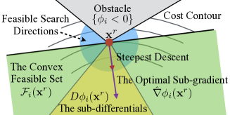
(a) Case one.

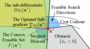
(b) Case two.

Figure 3: The choice of sub-gradient $\hat{\nabla}\phi_{i}(\mathbf{x}^{r})$ on non-smooth point $\mathbf{x}^{r}$.

4 Properties of the Convex Feasible Set Algorithm

This section shows the feasibility and convergence of Algorithm 1. The main result is summarized in the following theorem:

Theorem 4.1 (Convergence of Algorithm 1).

Under Algorithm 1, the sequence $\{\mathbf{x}^{(k)}\}$ will converge to some $\mathbf{x}^{*}\in\Gamma$ for any initial guess $\mathbf{x}^{(0)}$ such that $\mathcal{F}^{(0)}\neq\emptyset$. $\mathbf{x}^{*}$ is a strong local optimum of Eq. 1 if the limit is attained, i.e., there exists a constant $K\in\mathbb{N}$ such that $\mathbf{x}^{(k)}=\mathbf{x}^{*}$ for all $k>K$. $\mathbf{x}^{*}$ is at least a weak local optimum of Eq. 1 if the limit is not attained.

We say that $\mathbf{x}^{*}$ is a strong local optimum of Eq. 1 if $J$ is nondecreasing along any feasible search direction, e.g., $\nabla J(\mathbf{x}^{*})v\geq 0$ for all $v\in C(\mathbf{x}^{*})$ as shown in Fig. 4a. We say that $\mathbf{x}^{*}$ is a weak local optimum of Eq. 1 if the KKT condition is satisfied for some sub-gradients, i.e., $\nabla J(\mathbf{x}^{*})+\sum_{i=1}^{N}\lambda_{i}d_{i}=0$ for some $d_{i}\in D\phi_{i}(\mathbf{x}^{*})$ as shown in Fig. 4b. $\lambda_{i}$ is a Lagrange multiplier such that $\lambda_{i}\leq 0$ and $\lambda_{i}\phi_{i}(\mathbf{x})=0$ (complementary slackness) for all $i=1,\cdots,N$. A strong local optimum is always a weak local optimum. The two are equivalent when all $\phi_{i}$’s are smooth at $\mathbf{x}^{*}$.

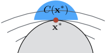
(a) A strong local optimum.

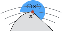
(b) A weak local optimum.

Figure 4: Definition of local optima.

4.1 Preliminary Results

Before proving Theorem 4.1, we present some preliminary results that are useful toward proving the theorem. Lemma 4.2 states that given a feasible reference point $\mathbf{x}^{r}$, $\mathcal{F}(\mathbf{x}^{r})$ is a convex set containing $\mathbf{x}^{r}$ with nontrivial interior. This conclusion naturally leads to the hypothesis that a suboptimal reference $\mathbf{x}^{r}$ can be improved by optimizing $J$ in the convex feasible set $\mathcal{F}(\mathbf{x}^{r})$. We will show in Proposition 4.4 that if the solution can not be improved using Algorithm 1, then $\mathbf{x}^{r}$ is already a strong local optimum of Eq. 1. Otherwise, if we can keep improving the result using Algorithm 1, this process will generate a Cauchy sequence that converges to a weak local optimum of Eq. 1, which will be shown in Proposition 4.9. Given these results, the conclusion in the theorem follows naturally.

The interior of a set $S$ is denoted as $S^{o}$. We say that a reference point $\mathbf{x}^{r}\in\mathbb{R}^{n}$ is feasible if $\mathbf{x}^{r}\in\Gamma$; and $\mathbf{x}^{*}\in\Gamma$ is a fixed point of Algorithm 1 if

(20) $$\mathbf{x}^{*}=\arg\min_{\mathbf{x}\in\mathcal{F}{(\mathbf{x}^{*})}}J(\mathbf{x}).$$

Lemma 4.2 (Feasibility).

If $\mathbf{x}^{r}\in\Gamma$, then $\mathbf{x}^{r}\in\mathcal{F}(\mathbf{x}^{r})$ and $\mathcal{F}^{o}(\mathbf{x}^{r})\neq\emptyset$.

Proof 4.3.

When $\mathbf{x}^{r}$ is feasible, $\mathbf{x}^{r}\in\mathcal{F}_{i}(\mathbf{x}^{r})$ for all $i$ according to the definitions in Eq. 15, Eq. 16 and Eq. 17. Hence $\mathbf{x}^{r}\in\mathcal{F}(\mathbf{x}^{r})$.

Claim 1: if $\mathbf{x}^{r}\in\Gamma^{o}$, then $\mathbf{x}^{r}\in\mathcal{F}^{o}(\mathbf{x}^{r})$. The condition $\mathbf{x}^{r}\in\Gamma^{o}$ implies that $\phi_{i}(\mathbf{x}^{r})>0$ for all $i=1,\cdots,N$. Then the inequality in Eq. 16 and Eq. 17 are not tight at $\mathbf{x}^{r}$. Hence $\mathbf{x}^{r}\in\mathcal{F}_{i}^{o}(\mathbf{x}^{r})$ in either of the three cases. Since $N$ is finite, $\mathbf{x}^{r}\in\bigcap_{i=1}^{N}\mathcal{F}_{i}^{o}(\mathbf{x}^{r})=\mathcal{F}^{o}(\mathbf{x}^{r})$.

Claim 2: if $\mathbf{x}^{r}\in\partial\Gamma$, there exists a non trivial $v\in\mathbb{R}^{n}$ such that $\mathbf{x}^{r}+v\in\mathcal{F}^{o}(\mathbf{x}^{r})$. Let $I:=\{i:\phi_{i}(x^{r})=0\}$. By the third statement in 2.2, there exists a unit vector $w\in\mathbb{R}^{n}$ such that $\partial_{w}\phi_{i}(\mathbf{x}^{r})<0$ for all $i\in I$. Fix $i\in I$. Let $a>0$ be sufficiently small. When $\phi_{i}$ is concave,

$$\phi_{i}(\mathbf{x}^{r}-aw)\geq\partial_{-aw}\phi_{i}(\mathbf{x}^{r})-\frac{a^{2}}{2}w^{T}H_{i}^{*}w\geq-a\partial_{w}\phi_{i}(\mathbf{x}^{r})-\frac{a^{2}}{2}w^{T}H_{i}^{*}w>0,$$

where the first inequality is due to semi-convexity, the second inequality is due to Eq. 7, and the third inequality is because $a$ is small. When $\phi_{i}$ is convex,

$$\phi_{i}(\mathbf{x}^{r})+\hat{\nabla}\phi_{i}(\mathbf{x}^{r})\cdot(-aw)\geq-a\partial_{w}\phi_{i}(\mathbf{x}^{r})>0,$$

where the first inequality is due to $\hat{\nabla}\phi_{i}(\mathbf{x}^{r})\cdot w\leq\partial_{w}\phi_{i}(\mathbf{x}^{r})$ by definition Eq. 11. When $\phi_{i}$ is neither concave nor convex,

$$\phi_{i}(\mathbf{x}^{r})+\hat{\nabla}\phi_{i}(\mathbf{x}^{r})\cdot(-aw)\geq-a\partial_{w}\phi_{i}(\mathbf{x}^{r})>\frac{a^{2}}{2}w^{T}H_{i}^{*}w.$$

Hence $\mathbf{x}^{r}-aw\in\mathcal{F}^{o}_{i}(\mathbf{x}^{r})$ for any sufficiently small $a$. Since $I$ is finite, we can find a constant $\epsilon$ such that $\mathbf{x}^{r}-aw\in\mathcal{F}^{o}_{i}(\mathbf{x}^{r})$ for all $i\in I$ and $0<a\leq\epsilon$. On the other hand, $\mathbf{x}^{r}\in\Gamma_{j}^{o}$ for all $j\notin I$. According to Claim 1, $\mathbf{x}^{r}\in\bigcap_{j\notin I}\mathcal{F}_{j}^{o}(\mathbf{x}^{r})$. There exists a constant $\epsilon_{0}>0$ such that $B(\mathbf{x}^{r},\epsilon_{0})\subset\bigcap_{j\notin I}\mathcal{F}_{j}^{o}(\mathbf{x}^{r})$. Define $v=-\min(\epsilon_{0},\epsilon)w$. According to previous discussion, $\mathbf{x}^{r}+v\in\mathcal{F}^{o}(\mathbf{x}^{r})$.

Claim 1 and Claim 2 imply that $\mathcal{F}(\mathbf{x}^{r})$ has nonempty interior.

Proposition 4.4 (Fixed point).

If $\mathbf{x}^{*}$ is a fixed point of Algorithm 1, then $\mathbf{x}^{*}$ is a strong local optimum of Eq. 1.

Proof 4.5.

We need to show that $\nabla J(\mathbf{x}^{*})\cdot v\geq 0$ for all $v\in C(\mathbf{x}^{*})$. If $\nabla J(\mathbf{x}^{*})=0$, then $\mathbf{x}^{*}$ is the global optimum of Eq. 1. Consider the case $\nabla J(\mathbf{x}^{*})\neq 0$. Claim that $\mathbf{x}^{*}\in\partial\Gamma$. First of all, since $\mathbf{x}^{*}\in\mathcal{F}(\mathbf{x}^{*})\subset\Gamma$, $\mathbf{x}^{*}$ is a feasible point. Moreover, since $J$ is strictly convex, the optimal point $\mathbf{x}^{*}$ must be on the boundary of $\mathcal{F}(\mathbf{x}^{*})$, i.e., $\mathbf{x}^{*}\in\partial\mathcal{F}_{i}(\mathbf{x}^{*})$ for some $i$. According to Eq. 15, Eq. 16 and Eq. 17, $\partial\mathcal{F}_{i}(\mathbf{x}^{*})$ equals to $\{\mathbf{x}:\phi_{i}(\mathbf{x})=0\}$ in case 1, $\{\mathbf{x}:\phi_{i}(\mathbf{x}^{*})+\hat{\nabla}\phi_{i}(\mathbf{x}^{*})(\mathbf{x}-\mathbf{x}^{*})=0\}$ in case 2, and $\{\mathbf{x}:\phi_{i}(\mathbf{x}^{*})+\hat{\nabla}\phi_{i}(\mathbf{x}^{*})(\mathbf{x}-\mathbf{x}^{*})=\frac{1}{2}(\mathbf{x}-\mathbf{x}^{*})^{T}H^{*}_{i}(\mathbf{x}-\mathbf{x}^{*})\}$ in case 3. Then $\mathbf{x}^{*}\in\partial\mathcal{F}_{i}(\mathbf{x}^{*})$ implies that $\phi_{i}(\mathbf{x}^{*})=0$. Hence $\mathbf{x}^{*}\in\partial\Gamma$. Let $I=\{i:\phi_{i}(\mathbf{x}^{*})=0\}=\{i:\mathbf{x}^{*}\in\partial\mathcal{F}_{i}(\mathbf{x}^{*})\}$.

Consider $v^{*}:=\arg\min_{v\in C(\mathbf{x}^{*})}\nabla J(\mathbf{x}^{*})\cdot v$. If the minimum is not unique, use the tie breaking mechanism discussed in Section 3.3. Claim that $\hat{\nabla}\phi_{i}\cdot v^{*}\geq 0$ for all $i\in I$. For $i\in I$ such that $\phi_{i}$ is smooth at $\mathbf{x}^{*}$, the definition of $C(\mathbf{x}^{*})$ implies that $\hat{\nabla}\phi_{i}(\mathbf{x}^{*})\cdot v^{*}=\nabla\phi_{i}(\mathbf{x}^{*})\cdot v^{*}\geq 0$. For $i\in I$ such that $\phi_{i}$ is not smooth at $\mathbf{x}^{*}$, $\hat{\nabla}\phi_{i}(\mathbf{x}^{*})\cdot v^{*}\geq 0$ since $\hat{\nabla}\phi_{i}\in DF_{i}:=\{d\in D\phi_{i}|d\cdot v^{*}\geq 0\}$. On the other hand, since $\mathbf{x}^{*}$ is the optimal solution of the smooth optimization $\min_{\mathbf{x}\in\mathcal{F}(\mathbf{x}^{*})}J(\mathbf{x})$ , the KKT condition is satisfied,

$$\nabla J(\mathbf{x}^{*})+\sum_{i=1}^{N}\lambda_{i}\hat{\nabla}\phi_{i}(\mathbf{x}^{*})=0.$$

The complementary slackness condition implies that $\lambda_{i}\leq 0$ for $i\in I$ and $\lambda_{j}=0$ for $j\notin I$. Hence

$$\nabla J(\mathbf{x}^{*})\cdot v^{*}=-\sum_{i=1}^{N}\lambda_{i}\hat{\nabla}\phi_{i}(\mathbf{x}^{*})\cdot v^{*}=-\sum_{i\in I}\lambda_{i}\hat{\nabla}\phi_{i}(\mathbf{x}^{*})\cdot v^{*}\geq 0.$$

Thus $J(\mathbf{x}^{*})\cdot v\geq 0$ for all $v\in C(\mathbf{x}^{*})$. So $\mathbf{x}^{*}$ is a strong local optimum of Eq. 1.

Remark 4.6.

Lemma 4.2 and Proposition 4.4 imply that a feasible $\mathbf{x}^{r}$ can always be improved by optimizing over the convex feasible set $\mathcal{F}(\mathbf{x}^{r})$ if $\mathbf{x}^{r}$ itself is not a strong local optimum. However, the existence of nonempty convex feasible set for an infeasible reference point is more intricate, which is deeply related to the choice of the functions $\phi_{i}$’s. The design considerations of $\phi_{i}$’s such that a nonempty convex feasible set always exists will be addressed in Section 5.

Lemma 4.7 (Strong descent).

For any feasible $\mathbf{x}^{(k)}$, the descent of the objective function satisfies that $\nabla J(\mathbf{x}^{(k+1)})(\mathbf{x}^{(k)}-\mathbf{x}^{(k+1)})\geq 0$. Moreover, if $J(\mathbf{x}^{(k+1)})=J(\mathbf{x}^{(k)})$, then $\mathbf{x}^{(k+1)}=\mathbf{x}^{(k)}$.

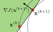
Figure 5: The descent of the sequence $\{\mathbf{x}^{(k)}\}$.

Proof 4.8.

Claim that $\mathcal{F}(\mathbf{x}^{(k)})$ is a subset of the half space $H:=\{\mathbf{x}\mid\nabla J(\mathbf{x}^{(k+1)})\cdot(\mathbf{x}-\mathbf{x}^{(k+1)})\geq 0\}$ as shown by the shaded area in Fig. 5. If not, there must be some $\hat{\mathbf{x}}\in\mathcal{F}(\mathbf{x}^{(k)})$ such that $\nabla J(\mathbf{x}^{(k+1)})\cdot(\hat{\mathbf{x}}-\mathbf{x}^{(k+1)})<0$. Let $v:=\hat{\mathbf{x}}-\mathbf{x}^{(k+1)}$. Since $\mathcal{F}(\mathbf{x}^{(k)})$ is convex, then $\mathbf{x}^{(k+1)}+av\in\mathcal{F}(\mathbf{x}^{(k)})$ for $a\in[0,1]$. Since $J$ is smooth, there exists a positive constant $c>0$ such that $J(\mathbf{x}^{(k+1)}+av)\leq J(\mathbf{x}^{(k+1)})+a\nabla J(\mathbf{x}^{(k+1)})\cdot v+ca^{2}\|v\|^{2}$. When $a$ is sufficiently small, the right-hand side of the inequality is strictly smaller than $J(\mathbf{x}^{(k+1)})$. Then $J(\mathbf{x}^{(k+1)}+av)<J(\mathbf{x}^{(k+1)})$, which contradicts with the fact that $\mathbf{x}^{(k+1)}$ is the minimum of $J$ in the convex feasible set $\mathcal{F}(\mathbf{x}^{(k)})$. Hence the claim is true. Since $\mathbf{x}^{(k)}\in\mathcal{F}(\mathbf{x}^{(k)})\subset H$, then $\nabla J(\mathbf{x}^{(k+1)})(\mathbf{x}^{(k)}-\mathbf{x}^{(k+1)})\geq 0$. Moreover, since $J$ is strictly convex, $J(\mathbf{x})>J(\mathbf{x}^{(k+1)})$ for all $\mathbf{x}\in H\setminus\{\mathbf{x}^{(k+1)}\}$. Hence $J(\mathbf{x}^{(k+1)})=J(\mathbf{x}^{(k)})$ implies $\mathbf{x}^{(k)}=\mathbf{x}^{(k+1)}$.

Proposition 4.9 (Convergence of strictly descending sequence).

Consider the sequence $\{\mathbf{x}^{(k)}\}$ generated by Algorithm 1. If $J(\mathbf{x}^{(1)})>J(\mathbf{x}^{(2)})>\cdots$, then the sequence $\{\mathbf{x}^{(k)}\}$ converges to a weak local optimum $\mathbf{x}^{*}$ of Eq. 1.

Proof 4.10.

The monotone sequence $\{J(\mathbf{x}^{(k)})\}_{i=2}^{\infty}$ converges to some value $a\geq\min J$. If $a=\min J$, the sequence $\{\mathbf{x}^{(k)}\}$ converges to the global optima. Consider the case $a>\min J$. Since $J$ is strictly convex by Eq. 1, the set $\{\mathbf{x}:J(\mathbf{x})\leq J(\mathbf{x}^{(1)})\}$ is compact. Then there exists a subsequence of $\{\mathbf{x}^{(k)}\}$ that converges to $\mathbf{x}^{*}$ such that $J(\mathbf{x}^{*})=a$. Since $\Gamma$ is closed, $\mathbf{x}^{*}\in\Gamma$.

We need to show that the whole sequence $\{\mathbf{x}^{(k)}\}$ converges to $\mathbf{x}^{*}$. Suppose not, then there exists $\delta>0$ such that $\forall K>0$, there exists $k>K$ s.t. $\|\mathbf{x}^{(k)}-\mathbf{x}^{*}\|\geq\delta$. For any $\epsilon\in(0,\delta)$, there exists $k,j\in\mathbb{N}$ such that $\|\mathbf{x}^{(k)}-\mathbf{x}^{*}\|\leq\epsilon$ and $\|\mathbf{x}^{(k+j)}-\mathbf{x}^{*}\|\geq\delta$. Since $J$ is strictly convex, there exists $c>0$ such that

$$J(\mathbf{x}^{(k)}) \geq J(\mathbf{x}^{(k+1)})+\nabla J(\mathbf{x}^{(k+1)})(\mathbf{x}^{(k)}-\mathbf{x}^{(k+1)})+c\|\mathbf{x}^{(k)}-\mathbf{x}^{(k+1)}\|^{2}$$

$$\geq J(\mathbf{x}^{(k+1)})+c\|\mathbf{x}^{(k)}-\mathbf{x}^{(k+1)}\|^{2}$$

$$\geq J(\mathbf{x}^{(k+j)})+c\|\mathbf{x}^{(k+j-1)}-\mathbf{x}^{(k+j)}\|^{2}+\cdots+\|\mathbf{x}^{(k)}-\mathbf{x}^{(k+1)}\|^{2}$$

$$\geq J(\mathbf{x}^{(k+j)})+c\|\mathbf{x}^{(k)}-\mathbf{x}^{(k+j)}\|^{2}$$

$$\geq J(\mathbf{x}^{(k+j)})+c(\|\mathbf{x}^{(k)}-\mathbf{x}^{*}\|-\|\mathbf{x}^{(k+j)}-\mathbf{x}^{*}\|)^{2}$$

$$\geq a+c(\delta-\epsilon)^{2},$$

which contradicts with the fact that $J(\mathbf{x}^{(k)})\rightarrow a$ as $\epsilon\rightarrow 0$. Note that the second inequality is due to $\nabla J(\mathbf{x}^{(k+1)})(\mathbf{x}^{(k)}-\mathbf{x}^{(k+1)})\geq 0$ in Lemma 4.7. The third inequality is by induction. The fourth inequality and the fifth inequality follow from $\Delta$-inequality. Hence we conclude that $\lim_{k\rightarrow\infty}\mathbf{x}^{(k)}=\mathbf{x}^{*}$.

Then we need to show that $\mathbf{x}^{*}$ is a weak local optimum. The proof can be divided into two steps. First, we show that there is a subsequence of the convex feasible sets $\{\mathcal{F}^{(k)}\}$ that converges point-wise to a suboptimal convex feasible set $\mathcal{G}$ at point $\mathbf{x}^{*}$. Sub-optimality of $\mathcal{G}$ means that the sub-gradients are not chosen according to Section 3.3. Then we show that $\mathbf{x}^{*}$ is the minimum of $J$ in $\mathcal{G}$. Thus the KKT condition is satisfied at $\mathbf{x}^{*}$ and $\mathbf{x}^{*}$ is a weak local optimum of Eq. 1.

Consider any $\phi_{i}$. If $\phi_{i}$ is smooth at $\mathbf{x}^{*}$, then it is smooth in a neighborhood of $\mathbf{x}^{*}$ as $\phi_{i}$ is assumed to be piece-wise smooth. Then $\hat{\nabla}\phi_{i}(\mathbf{x}^{(k)})$ converges to $d_{i}:=\nabla\phi_{i}(\mathbf{x}^{*})$. If $\phi_{i}$ is not smooth at $\mathbf{x}^{*}$, it is still locally Lipschitz due to semi-convexity. Then $\hat{\nabla}\phi_{i}$ is locally bounded. Hence there is a subsequence $\{\hat{\nabla}\phi_{i}(\mathbf{x}^{(k_{j})})\}_{k_{j}\in\mathbb{N}}$ that converges to some $d_{i}\in\mathbb{R}^{n}$. Claim that $d_{i}\in D\phi_{i}(\mathbf{x}^{*})$. By definition Eq. 11, for any $v\in\mathbb{R}^{n}$, $\hat{\nabla}\phi_{i}(\mathbf{x}^{(k_{j})})\cdot v\leq\partial_{v}\phi_{i}(\mathbf{x}^{(k_{j})})$. Since $\phi_{i}$ is piecewise smooth, then either $\partial_{v}\phi_{i}(\mathbf{x}^{(k_{j})})\rightarrow\partial_{v}\phi_{i}(\mathbf{x}^{*})$ or $\partial_{v}\phi_{i}(\mathbf{x}^{(k_{j})})\rightarrow-\partial_{-v}\phi_{i}(\mathbf{x}^{*})$. Since $-\partial_{-v}\phi_{i}(\mathbf{x}^{*})\leq\partial_{v}\phi_{i}(\mathbf{x}^{*})$ by Eq. 7, we have the following inequality,

$$d_{i}\cdot v=\lim_{k_{j}\rightarrow\infty}\hat{\nabla}\phi_{i}(\mathbf{x}^{(k_{j})})\cdot v\leq\lim_{k_{j}\rightarrow\infty}\partial_{v}\phi_{i}(\mathbf{x}^{(k_{j})})\leq\partial_{v}\phi_{i}(\mathbf{x}^{*}).$$

Hence by definition Eq. 11, $d_{i}\in D\phi_{i}(\mathbf{x}^{*})$. Then we can choose a subsequence $\{\mathbf{x}^{(k_{n})}\}_{k_{n}\in\mathbb{N}}$ such that $\phi_{i}(\mathbf{x}^{(k_{n})})$ converges to $\phi_{i}(\mathbf{x}^{*})$ and $\hat{\nabla}\phi_{i}(\mathbf{x}^{(k_{n})})$ converges to $d_{i}\in D\phi_{i}(\mathbf{x}^{*})$ for all $i=1,\cdots,N$. For simplicity and without loss of generality, we use the same notation for the subsequence as the original sequence in the following discussion.

Define a new convex feasible set $\mathcal{G}_{i}$ such that $\mathcal{G}_{i}=\Gamma_{i}$ if $\phi_{i}$ is concave, $\mathcal{G}_{i}=\{\mathbf{x}:\phi_{i}(\mathbf{x}^{*})+d_{i}(\mathbf{x}-\mathbf{x}^{*})\geq 0\}$ if $\phi_{i}$ is convex, and $\mathcal{G}_{i}=\{\mathbf{x}:\phi_{i}(\mathbf{x}^{*})+d_{i}(\mathbf{x}-\mathbf{x}^{*})\geq\frac{1}{2}(\mathbf{x}-\mathbf{x}^{*})^{T}H^{*}_{i}(\mathbf{x}-\mathbf{x}^{*})\}$ if otherwise. Let $\mathcal{G}=\bigcap_{i=1}^{N}\mathcal{G}_{i}$.

Claim that $\mathcal{G}=\lim_{k\rightarrow\infty}\mathcal{F}^{(k)}$ where $\lim_{k\rightarrow\infty}\mathcal{F}^{(k)}:=\bigcap_{k\rightarrow\infty}\bigcup_{j=k}^{\infty}\mathcal{F}^{(k)}$. Consider $z\in\mathcal{G}$. If $\phi_{i}$ is concave, then $z\in\mathcal{F}_{i}^{(k)}:=\mathcal{F}_{i}(\mathbf{x}^{(k)})$ for all $k$ according to Eq. 16. If $\phi_{i}$ is convex, then

$$\lim_{k\rightarrow\infty}\left[\phi_{i}(\mathbf{x}^{(k)})+\hat{\nabla}\phi_{i}(\mathbf{x}^{(k)})(z-\mathbf{x}^{(k)})\right]=\phi_{i}(\mathbf{x}^{*})+d_{i}(z-\mathbf{x}^{*})\geq 0,$$

which implies that $z\in\lim_{k\rightarrow\infty}\mathcal{F}_{i}^{(k)}$. Similarly, we can show that if $\phi_{i}$ is neither convex or concave, $z$ also lies in the limit of $\mathcal{F}_{i}^{(k)}$. Hence $z\in\bigcap_{i=1}^{N}\lim_{k\rightarrow\infty}\mathcal{F}_{i}^{(k)}=\lim_{k\rightarrow\infty}\mathcal{F}^{(k)}$. Since $z$ is arbitrary, $\mathcal{G}\subset\lim_{k\rightarrow\infty}\mathcal{F}^{(k)}$. For any $z\in\lim_{k\rightarrow\infty}\mathcal{F}^{(k)}$, then there exists a sequence $\{z_{k}\}$ that converges to $z$ such that $z_{k}\in\mathcal{F}^{(k)}$. For any $i$, if $\phi_{i}$ is concave, then $z_{k}\in\mathcal{F}_{i}^{(k)}=\mathcal{G}_{i}$. Since $\mathcal{G}_{i}$ is closed, $z\in\mathcal{G}_{i}$. If $\phi_{i}$ is convex, then

$$\phi_{i}(\mathbf{x}^{*})+d_{i}(z-\mathbf{x}^{*})=\lim_{k\rightarrow\infty}\left[\phi_{i}(\mathbf{x}^{(k)})+\hat{\nabla}\phi_{i}(\mathbf{x}^{(k)})(z_{k}-\mathbf{x}^{(k)})\right]\geq 0,$$

which implies that $z\in\mathcal{G}_{i}$. Similarly, we can show that $z\in\mathcal{G}_{i}$ if $\phi_{i}$ is neither convex or concave. Hence $z\in\mathcal{G}$. And we verify that $\mathcal{G}=\lim_{k\rightarrow\infty}\mathcal{F}^{(k)}$.

Claim that $\mathbf{x}^{*}=\arg\min_{\mathbf{x}\in\mathcal{G}}J(\mathbf{x})$. Suppose not, then there exists $z\in\mathcal{G}$ such that $J(z)<J(\mathbf{x}^{*})$. For all $\epsilon>0$, there exists $y\in\mathcal{F}^{(k)}$ for some $k\in\mathbb{N}$ such that $\|z-y\|<\epsilon$. Since $J$ is smooth, then $J(y)-J(z)<O(\epsilon)$. Thus $J(y)<J(\mathbf{x}^{*})$ when $\epsilon$ is sufficiently small. This contradicts with $J(y)>J(\mathbf{x}^{(k)})>J(\mathbf{x}^{*})$. Hence $J(z)\geq J(\mathbf{x}^{*})$ for all $z\in\mathcal{G}$. If there exists $z\in\mathcal{G}\setminus\{\mathbf{x}^{*}\}$ such that $J(z)=J(\mathbf{x}^{*})$, then $\frac{z+\mathbf{x}^{*}}{2}\in\mathcal{G}$ and $J(\frac{z+\mathbf{x}^{*}}{2})<\frac{J(z)+J(\mathbf{x}^{*})}{2}=J(\mathbf{x}^{*})$ since $\mathcal{G}$ is convex and $J$ is strictly convex. However, this contradicts with the conclusion that $J(z)\geq J(\mathbf{x}^{*})$ for all $z\in\mathcal{G}$. Hence $\mathbf{x}^{*}$ is the unique minimum of $J$ in the set $\mathcal{G}$. And the KKT condition is satisfied, i.e., $\nabla J(\mathbf{x}^{*})+\sum_{i=1}^{N}\lambda_{i}d_{i}=0$ for $d_{i}\in D\phi_{i}(\mathbf{x}^{*})$. Then $\mathbf{x}^{*}$ is a weak local optimum.

It is worth noting that if all $\phi_{i}$’s are smooth at $\mathbf{x}^{*}$, $\mathcal{G}=\mathcal{F}(\mathbf{x}^{*})$. Then $\mathbf{x}^{*}$ is a fixed point, thus a strong local optimum by Proposition 4.4.

Remark 4.11.

Lemma 4.7 and Proposition 4.9 justify the adoption of the terminate condition Eq. 14, which is indeed equivalent to the standard terminate condition Eq. 13, e.g., convergence in the objective function implies convergence in the solution.

4.2 Proof of the Main Result

Proof 4.12 (Proof of Theorem 4.1).

If $\mathcal{F}^{(0)}$ is nonempty, then $\mathbf{x}^{(1)}\in\Gamma$ can be obtained by solving the convex optimization Eq. 12. By Lemma 4.2, $\mathcal{F}^{(1)}$ has nonempty interior, then $\mathbf{x}^{(2)}\in\Gamma$ can be obtained. By induction, we can conclude that $\mathbf{x}^{(i)}\in\mathcal{F}^{(i-1)}\subset\Gamma$ for $i=1,2,3,\cdots$. Moreover, as a better solution is found at each iteration, then $J(\mathbf{x}^{(1)})\geq J(\mathbf{x}^{(2)})\geq\cdots$. This leads to two cases. The first case is that $J(\mathbf{x}^{(K)})=J(\mathbf{x}^{(K+1)})$ for some $K$, while the second case is that the cost keeps decreasing strictly, i.e., $J(\mathbf{x}^{(1)})>J(\mathbf{x}^{(2)})>\cdots$. In the first case, the condition $J(\mathbf{x}^{(K)})=J(\mathbf{x}^{(K+1)})$ is equivalent to $\mathbf{x}^{(K)}=\mathbf{x}^{(K+1)}$ by Lemma 4.7. By induction, the algorithm converges in the sense that $\mathbf{x}^{(k)}=\mathbf{x}^{(k+1)}$ and $J(\mathbf{x}^{(k)})=J(\mathbf{x}^{(k+1)})$ for all $k\geq K$. Moreover, as $\mathbf{x}^{*}:=\mathbf{x}^{(K)}$ is a fixed point, it is a strong local optimum by Proposition 4.4. If the cost keeps decreasing, e.g., $J(\mathbf{x}^{(1)})>J(\mathbf{x}^{(2)})>\cdots$, then the sequence $\{\mathbf{x}^{(k)}\}$ converges to a weak local optimum $\mathbf{x}^{*}$ by Proposition 4.9.

5 Application on Motion Planning for Mobile Robots

In this section, Algorithm 1 is applied to a motion planning problem for mobile robots [25]. Its application to other systems can be found in [16]. The problem will be formulated in Section 5.1 and then transformed into the benchmark form Eq. 1 and Eq. 2. The major difficulty in transforming the problem lies in finding the semi-convex function $\phi_{i}$ to describe the constraints. The method to construct $\phi_{i}$ in 2D is discussed in Section 5.2 and the resulting convex feasible set is illustrated through examples in Section 5.3. The performance of Algorithm 1 is shown in Section 5.4 and compared to interior point method (ITP) and sequential quadratic programming (SQP).

5.1 Problem Statement

Suppose a mobile robot needs to plan a trajectory in $\mathbb{R}^{2}$ from the start point $x_{0}$ to the goal point $G$ as shown in Fig. 6. Let $x_{q}\in\mathbb{R}^{2}$ be the position of the robot at time step $q$. Define the decision variable as $\mathbf{x}:=\left[\begin{array}[]{ccc}x_{1}^{T}&\cdots&x_{h}^{T}\end{array}\right]^{T}\in\mathbb{R}^{2h}$ where $h$ is the planning horizon. The whole trajectory is denoted as $\bar{\mathbf{x}}:=\left[\begin{array}[]{ccc}x_{0}^{T}&\mathbf{x}^{T}&G^{T}\end{array}\right]^{T}\in\mathbb{R}^{2(h+2)}$. Define a sequence of selection functions $l_{q}:\mathbb{R}^{2h}\rightarrow\mathbb{R}^{2}$ as $x_{q}=l_{q}(\mathbf{x})$. The sampling time is $t_{s}$. Let the velocity at $q$ be $v_{q}:=\frac{x_{q}-x_{q-1}}{t_{s}}$ and the acceleration at $q$ be $a_{q}:=\frac{v_{q}-v_{q-1}}{t_{s}}$.

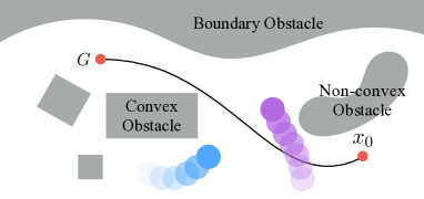
Figure 6: The motion planning problem.

The Cost Function

The cost function of the problem is designed as

(21) $$J(\mathbf{x})=w_{1}\|\mathbf{x}-\mathbf{x}^{r}\|^{2}_{Q}+w_{2}\|\mathbf{x}\|^{2}_{S},$$

where $w_{1},w_{2}\in\mathbb{R}^{+}$. The first term $\|\mathbf{x}-\mathbf{x}^{r}\|^{2}_{Q}:=(\bar{\mathbf{x}}-\bar{\mathbf{x}}^{r})^{T}Q(\bar{\mathbf{x}}-\bar{\mathbf{x}}^{r})$ penalizes the distance from the target trajectory to the reference trajectory. The second term $\|\mathbf{x}\|^{2}_{S}:=\bar{\mathbf{x}}^{T}S\bar{\mathbf{x}}$ penalizes the properties of the target trajectory itself, e.g., length of the trajectory and magnitude of acceleration. The matrices $Q,S\in\mathbb{R}^{2(h+2)\times 2(h+2)}$ can be constructed from the following components: 1) matrix for position $Q_{1}:=I_{2(h+2)}$; 2) matrix for velocity $Q_{2}:=V^{T}V$ and 3) matrix for acceleration $Q_{3}:=A^{T}A$. Note that $V\in\mathbb{R}^{2(h+1)\times 2(h+2)}$ and $A\in\mathbb{R}^{2h\times 2(h+2)}$ are defined as

$$V=\footnotesize{\frac{1}{t_{s}}\left[\begin{array}[]{ccccc}I_{2}&-I_{2}&0&\cdots&0\\ 0&I_{2}&-I_{2}&\cdots&0\\ \vdots&\vdots&\ddots&\ddots&\vdots\\ 0&0&\cdots&I_{2}&-I_{2}\end{array}\right]},A=\frac{1}{t_{s}^{2}}\left[\begin{array}[]{cccccc}I_{2}&-2I_{2}&I_{2}&0&\cdots&0\\ 0&I_{2}&-2I_{2}&I_{2}&\cdots&0\\ \vdots&\vdots&\ddots&\ddots&\ddots&\vdots\\ 0&0&\cdots&I_{2}&-2I_{2}&I_{2}\end{array}\right],$$

which take finite differences of the trajectory $\mathbf{x}$ such that $V\mathbf{x}$ returns the velocity vector and $A\mathbf{x}$ returns the acceleration vector. Then $Q:=\sum_{i=1}^{3}c^{q}_{i}Q_{i}$ and $S:=\sum_{i=1}^{3}c^{s}_{i}Q_{i}$ where $c^{q}_{i}$ and $c^{s}_{i}$ are positive constants. Eq. 1 is satisfied.

The Constraints

The obstacles in the environment are denoted as $\mathcal{O}_{j}\in\mathbb{R}^{2}$ for $j\in\mathbb{N}$. Each $\mathcal{O}_{j}$ is simply connected and open with piecewise smooth boundary that does not contain any sharp concave corner. For example, there are seven such obstacles in Fig. 6 where five of them are static and two are dynamic. Let $\mathcal{O}_{j}$ denote obstacle $j$ when centered at the origin. The area occupied by obstacle $j$ at time step $q$ is defined as $\mathcal{O}_{j}(q)$. Define a linear isometry $\mathcal{T}_{j,q}:\mathbb{R}^{2}\rightarrow\mathbb{R}^{2}$ such that $\mathcal{O}_{j}=\mathcal{T}_{j,q}(\mathcal{O}_{j}(q))$. Then $x_{q}\notin\mathcal{O}_{j}(q)$ is equivalent to $\mathcal{T}_{j,q}(x_{q})\notin\mathcal{O}_{j}$. Hence the constraint for the optimization is

(22) $$\mathbf{x}\in\Gamma:=\{\mathbf{x}\in\mathbb{R}^{2h}:\mathcal{T}_{j,q}(l_{q}(\mathbf{x}))\notin\mathcal{O}_{j},\forall j,\forall q=1,\cdots,h\}.$$

It is easy to verify that Eq. 1 is satisfied.

5.2 Transforming the Problem

In order to apply Algorithm 1, a semi-convex decomposition Eq. 2 satisfying 2.2 needs to be performed. For example, obstacles containing concave corners need to be partitioned into several overlapping obstacles that do not have concave corners as discussed in Section 2.2. Without loss of generality, $\mathcal{O}_{j}$ is assumed to represent obstacles after decomposition such that it is either a convex obstacle, or a boundary obstacle, or a non-convex obstacle as shown in Fig. 6. For each $\mathcal{O}_{j}$, we first construct a simple function $\varphi_{j}:\mathbb{R}^{2}\rightarrow\mathbb{R}$ and then use $\varphi_{j}$ to construct $\phi_{i}$. The function $\varphi_{j}$ is continuous, piecewise smooth and semi-convex such that $\mathcal{O}_{j}=\{x\in\mathbb{R}^{2}:\varphi_{j}(x)<0\}$ and $\partial\mathcal{O}_{j}=\{x\in\mathbb{R}^{2}:\varphi_{j}(x)=0\}$. We call $\varphi_{j}$ a safety index in the following discussion, since it typically measures the distance to an obstacle. The construction of $\varphi_{j}$ in each case is discussed below.

Convex obstacle

A convex obstacle refers to the case that $\mathcal{O}_{j}$ is compact and convex. In this case, $\varphi_{j}$ is defined to be the signed distance function to $\mathcal{O}_{j}$, i.e.,

(23) $$\varphi_{j}(x):=\left\{\begin{array}[]{ll}\min_{y\in\partial\mathcal{O}_{j}}\|x-y\|&x\notin\mathcal{O}_{j}\\ -\min_{y\in\partial\mathcal{O}_{j}}\|x-y\|&x\in\mathcal{O}_{j}\end{array}\right..$$

Boundary obstacle

A boundary obstacle refers to a non-compact $\mathcal{O}_{j}$ such that there is an affine parameterization of $\partial\mathcal{O}_{j}$, e.g., if we rotate and align the obstacle properly, there exists a continuous and piecewise smooth semi-convex function $f:\mathbb{R}\rightarrow\mathbb{R}$ such that $p_{2}=f(p_{1})$ describes $\partial\mathcal{O}_{j}$ where $x=(p_{1},p_{2})\in\mathbb{R}^{2}$. Then $\varphi_{j}$ is defined as the directional distance along $(0,1)$ to the boundary $\partial\mathcal{O}_{j}$, i.e.,

(24) $$\varphi_{j}(x):=f(p_{1})-p_{2}.$$

Non-convex obstacle

A non-convex obstacle refers to the case that $\mathcal{O}_{j}$ is compact, but non-convex. As the signed distance function for a non-convex set is not semi-convex, the strategy is to introduce directional distance. Denote the smallest convex envelop of the obstacle $\mathcal{O}_{j}$ as $\widehat{\mathcal{O}}_{j}$. Then $\varphi_{j}$ is defined as a signed directional distance function which computes the minimum distance from a point $x$ to $\partial\mathcal{O}_{j}$ in the direction that is perpendicular to $\partial\widehat{\mathcal{O}}_{j}$ as shown in Fig. 7b. Let $\delta$ be a correspondence function that maps a point $y\in\partial\widehat{\mathcal{O}}_{j}$ to the closest $z\in\partial\mathcal{O}_{j}$ such that $z-y$ is perpendicular to $\partial\widehat{\mathcal{O}}_{j}$ at $y$. It is assumed that $\delta$ is bijective and $\|y-\delta(y)\|$ is semi-convex in $y$. Then

(25) $$\varphi_{j}(x)=\left\{\begin{array}[]{ll}\min_{y\in\partial\widehat{\mathcal{O}}_{j}}[\|x-y\|+\|y-\delta(y)\|]&x\notin\widehat{\mathcal{O}}_{j}\\ -\min_{y\in\partial\widehat{\mathcal{O}}_{j}}[\|x-y\|-\|y-\delta(y)\|]&x\in\widehat{\mathcal{O}}_{j}\end{array}\right..$$

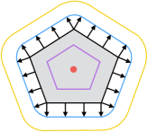
(a) Convex obstacle.

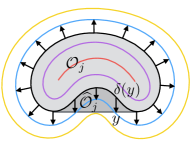
(b) Concave obstacle.

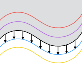
(c) Boundary obstacle.

Figure 7: Contours of the safety indices for typical obstacles.

It is easy to verify that $\varphi_{j}$ in all three cases are continuous, piecewise smooth, semi-convex, and satisfy the first two arguments in 2.2. Moreover, $\varphi_{j}$ is strictly convex for convex obstacles. According to Eq. 23, Eq. 24 and Eq. 25, the contours of the safety indices are shown in Fig. 7. Based on the safety indices, Eq. 22 can be re-written as

(26) $$\mathbf{x}\in\Gamma=\bigcap_{j,q}\{\mathbf{x}\in\mathbb{R}^{2h}:\varphi_{j}(\mathcal{T}_{j,q}(l_{q}(\mathbf{x})))\geq 0\}.$$

Define $\phi_{j,q}(\mathbf{x}):=\varphi_{j}(\mathcal{T}_{j,q}(l_{q}(\mathbf{x})))$ for all $j$ and $q$. Let $\Gamma_{j,q}:=\{\mathbf{x}\in\mathbb{R}^{2h}:\phi_{j,q}(\mathbf{x})\geq 0\}$. When the obstacles do not overlap with each other at every time step as shown in Fig. 6, the third argument in 2.2 is satisfied. Then $\{\phi_{j,q}\}_{j,q}$ is a decomposition of $\Gamma$ that satisfies 2.2. The convex feasible set $\mathcal{F}:=\bigcap_{j,q}\mathcal{F}_{j,q}$ can be constructed according to the discussion in Section 3.2. And Algorithm 1 can be applied.

5.3 The Convex Feasible Set - Examples

This section illustrates the configuration of convex feasible sets with examples. Since $\phi_{j,q}$ only depends on $x_{q}$, $\mathcal{F}_{j,q}(\mathbf{x}^{r})$ only constraint $x_{q}$. For example, according to Eq. 16, the convex feasible set for a convex $\phi_{j,q}$ is

(27) $$\mathcal{F}_{j,q}(\mathbf{x}^{r})=\{\mathbf{x}:\varphi_{j}(\mathcal{T}_{j,q}(x_{q}^{r}))+\hat{\nabla}\varphi_{j}(\mathcal{T}_{j,q}(x_{q}^{r}))\nabla\mathcal{T}_{j,q}(x_{q}^{r})(x_{q}-x_{q}^{r})\geq 0\}.$$

For simplicity, define $\mathcal{F}^{q}_{j,q}(\mathbf{x}^{r}):=l_{q}(\mathcal{F}_{j,q}(\mathbf{x}^{r}))\in\mathbb{R}^{2}$. In the following discussion, we will first illustrate $\mathcal{F}^{q}_{j,q}(\mathbf{x}^{r})$ in $\mathbb{R}^{2}$ and then $\bigcap_{q}\mathcal{F}_{j,q}(\mathbf{x}^{r})$ in $\mathbb{R}^{2h}$.

The convex feasible set in $\mathbb{R}^{2}$

We illustrate the convex feasible set for one obstacle at one time step. For simplicity, subscripts $j$ and $q$ are removed and $\mathcal{T}_{j,q}$ is assumed to be identity. Consider a polygon obstacle with vertices $a=(1,1)$, $b=(-1,1)$, $c=(-1,-1)$ and $d=(1,-1)$ as shown in Fig. 8a. Let $\|x\|_{\infty}$ denote the $l_{\infty}$ norm, i.e., $\|x\|_{\infty}:=\max\{|p_{1}|,|p_{2}|\}$. Then according to Eq. 23,

(28) $$\varphi(x)=\left\{\begin{array}[]{ll}\max\{-1-p_{1},p_{1}-1,p_{2}-1,-1-p_{2}\}&\|x\|_{\infty}\leq 1\\ \min\{\|x-a\|,\|x-b\|,\|x-c\|,\|x-d\|\}&|p_{1}|>1,|p_{2}|>1\\ \min\{|p_{1}-1|,|p_{1}+1|\}&|p_{1}|>1,|p_{2}|<1\\ \min\{|p_{2}-1|,|p_{2}+1|\}&|p_{1}|<1,|p_{2}|>1\end{array}\right..$$

For a reference point $x^{r}=(-1.5,-1.5)$, $\varphi(x^{r})=\frac{\sqrt{2}}{2}$ and $\nabla\varphi(x^{r})=\frac{\sqrt{2}}{2}[-1,-1]$. The convex feasible set is $\mathcal{F}(x^{r})=\{x:\varphi(x^{r})+\nabla\varphi(x^{r})(x-x^{r})\geq 0\}=\{x:\frac{\sqrt{2}}{2}(-p_{1}-p_{2}+2)\geq 0\}$. The bowl-shaped surface in Fig. 8a illustrates the safety index $\varphi$. The plane that is tangent to the safety index satisfies the function $\frac{\sqrt{2}}{2}(-p_{1}-p_{2}+2)=0$. Since $\varphi$ is convex, the tangent plane is always below $\varphi$. The convex feasible set can be regarded as the projection of the positive portion of the tangent plane onto the zero level set.

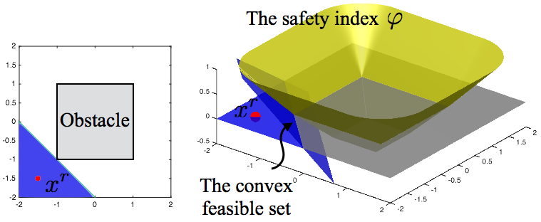
(a) Convex obstacle.

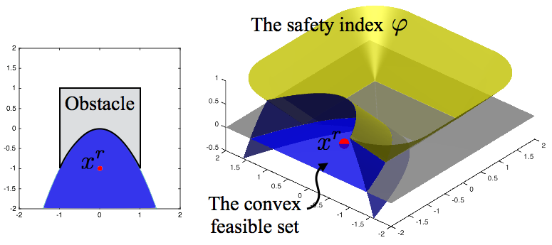
(b) Non-convex obstacle.

Figure 8: Illustration of the convex feasible set in $\mathbb{R}^{2}$.

Consider the case that points $c$ and $d$ are not connected by a straight line, but a concave curve $p_{2}=-(p_{1})^{2}$ as shown in Fig. 8b. Then according to Eq. 25,

(29) $$\varphi(x)=\left\{\begin{array}[]{ll}\max\{-(p_{1})^{2}-p_{2},p_{1}-1,p_{2}-1,-1-p_{2}\}&\|x\|_{\infty}\leq 1,p_{2}\geq-(p_{1})^{2}\\ \min\{\|x-a\|,\|x-b\|,\|x-c\|,\|x-d\|\}&|p_{1}|>1,|p_{2}|>1\\ \min\{|p_{1}-1|,|p_{1}+1|\}&|p_{1}|>1,|p_{2}|<1\\ p_{2}-1&p_{2}>1\\ -(p_{1})^{2}-p_{2}&p_{2}<-(p_{1})^{2}\end{array}\right..$$

The hessian of $\varphi$ is bounded below by $-H^{*}=[-2,0;0,0]$. For a reference point $x^{r}=(0,-1)$, $\varphi(x^{r})=1$ and $\nabla\varphi(x^{r})=[0,-1]$. The convex feasible set is $\mathcal{F}(x^{r})=\{x:\varphi(x^{r})+\nabla\varphi(x^{r})(x-x^{r})\geq\frac{1}{2}(x-x^{r})H^{*}(x-x^{r})\}=\{x:-p_{2}-(p_{1})^{2}\geq 0\}$. The bowl-shaped surface in Fig. 8b illustrates the safety index $\varphi$. The parabolic surface that is tangent to the safety index represents the function $-p_{2}-(p_{1})^{2}=0$. The convex feasible set is the projection of the positive portion of the surface onto the zero level set.

The convex feasible set in higher dimension

We illustrate the convex feasible set for one obstacle over the entire time horizon. The obstacle is shown in Fig. 9a, which is a translated version of the obstacle in Fig. 8a. The reference trajectory violates the obstacle avoidance constraint. Fig. 9b shows the convex feasible sets computed for each time step. Those sets formulate a corridor around the time-augmented obstacle. A new trajectory will be computed in the corridor. Although the projection of the corridor into $\mathbb{R}^{2}$ is not convex, each time slice of the corridor is convex. In $\mathbb{R}^{2h}$, those slices are sticked together orthogonally, hence formulate a convex subset of $\mathbb{R}^{2h}$.

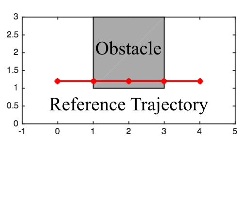
(a) The reference trajectory.

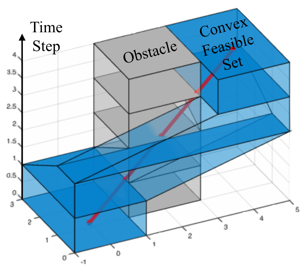
(b) The convex feasible set over time.

Figure 9: Illustration of the convex feasible set in $\mathbb{R}^{2h}$.

As pointed out in Remark 4.6, for an infeasible reference trajectory, when there are multiple obstacles, the existence of a corridor that bypasses all time-augmented obstacles under the proposed algorithm is hard to guarantee. In Lemma 5.1, we show that a convex feasible set has nonempty interior for any reference trajectory if certain geometric conditions are satisfied.

Lemma 5.1 (Feasibility).

If all obstacles are convex and have disjoint closures, i.e., $\bar{\mathcal{O}}_{i}(q)\bigcap\bar{\mathcal{O}}_{j}(q)=\emptyset$ for all $q$ and $i\neq j$, then the convex feasible set $\mathcal{F}(\mathbf{x}^{r})$ has nonempty interior for all $\mathbf{x}^{r}\in\mathbb{R}^{n}$ when $\phi_{j,q}$ is chosen according to Eq. 23 and Eq. 26.

Proof 5.2.

Considering Lemma 4.2, we only need to prove that $\mathcal{F}(\mathbf{x}^{r})$ has nonempty interior for infeasible $\mathbf{x}^{r}$. Infeasibility of $\mathbf{x}^{r}$ implies that some $\phi_{j,q}(\mathbf{x}^{r})$ is negative. Fix $q$, since $\bar{\mathcal{O}}_{j}(q)$’s are disjoint, only one $\phi_{j,q}$ can be negative. Without loss of generality, suppose $\phi_{1,q}(\mathbf{x}^{r})<0$ and $\phi_{j,q}(\mathbf{x}^{r})\geq 0$ for $j\geq 2$. Since the safety index $\varphi_{j}$ is a signed distance function in Eq. 23 and $\mathcal{T}_{j,q}$ is an isometry, $\|\hat{\nabla}\varphi_{j}\|=1$ and $\|\mathcal{T}_{j,q}\|=1$. Then the ball $B(x_{q}^{r},\varphi_{j}(\mathcal{T}_{j,q}(x_{q}^{r})))$ is a subset of $\mathcal{F}_{j,q}^{q}(\mathbf{x}^{r})$ according to Eq. 27 for all $j$ and $q$. Hence $B(x_{q}^{r},d^{*})\subset\bigcap_{j\geq 2}\mathcal{F}_{j,q}^{q}(\mathbf{x}^{r})$ where $d^{*}=\min_{j\geq 2}\varphi_{j}(\mathcal{T}_{j,q}(x_{q}^{r}))$ is the minimum distance to $\bigcup_{j\geq 2}\mathcal{O}_{j}(q)$. According to Eq. 23, $\mathcal{F}^{q}_{1,q}(\mathbf{x}^{r})$ is tangent to $\partial\mathcal{O}_{1}(q)$ at a point $x^{*}$ such that $\varphi_{1}(\mathcal{T}_{1,q}(x_{q}^{r}))=-\|x_{q}^{r}-x^{*}\|$ as shown in Fig. 10. Since $\bar{\mathcal{O}}_{1}(q)\bigcap\bar{\mathcal{O}}_{j}(q)=\emptyset$ for $j\geq 2$, then $d^{*}>-\varphi_{1}(\mathcal{T}_{1,q}(x_{q}^{r}))=\|x^{r}_{q}-x^{*}\|$, which implies that the set $\mathcal{F}_{1,q}^{q}(\mathbf{x}^{r})\bigcap B(x_{q}^{r},d^{*})$ has nonempty interior. Then $\bigcap_{j}\mathcal{F}^{q}_{j,q}(\mathbf{x}^{r})$ has nonempty interior. So $\mathcal{F}(\mathbf{x}^{r})=\oplus_{q}(\bigcap_{j}\mathcal{F}^{q}_{j,q}(\mathbf{x}^{r}))$ has nonempty interior where $\oplus$ means direct sum.

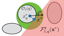
Figure 10: Existence of convex feasible set for an infeasible reference point.

Remark 5.3.

Lemma 5.1 implies that $\mathcal{F}^{(0)}$ is nonempty for any $\mathbf{x}^{(0)}$. By Theorem 4.1, the algorithm converges to a local optimum for any $\mathbf{x}^{(0)}\in\mathbb{R}^{n}$ if all obstacles are convex and have disjoint closures.

5.4 Performance and Comparison

The performance of Algorithm 1 will be illustrated through two examples, which will also be compared to the performance of existing non-convex optimization methods, interior point (ITP) and sequential quadratic programming (SQP). For simplicity, only convex obstacles and convex boundaries are considered. Algorithm 1 is implemented in both Matlab and C++. The convex optimization problem Eq. 12 is solved using the interior-point-convex method in quadprog in Matlab and the interior point method in Knitro [4] in C++. For comparison, Eq. 1 is also solved directly using ITP and SQP methods in fmincon [1] in Matlab and in Knitro in C++. To create fair comparison, the gradient and the hessian of the objective function $J$ and the optimal sub-gradients $\hat{\nabla}\phi_{i}$ of the constraint function $\phi_{i}$’s are also provided to ITP and SQP solvers.

In the examples, $x_{0}=(0,0)$ and $G=(9,0)$. The planning horizon $h$ goes from $30$ to $100$. $t_{s}=(h+1)^{-1}$. The cost function Eq. 21 penalizes the average acceleration along the trajectory, e.g., $Q=0$ and $S=h^{-1}A^{T}A$. When $h\rightarrow\infty$, $J(\mathbf{x})\rightarrow\int_{0}^{1}\|\ddot{\mathbf{x}}\|^{2}dt$ where $\mathbf{x}:[0,1]\rightarrow\mathbb{R}^{n}$ is a continuous trajectory with $\mathbf{x}(0)=x_{0}$ and $\mathbf{x}(1)=G$. The initial reference $\mathbf{x}^{(0)}$ is chosen to be a straight line connecting $x_{0}$ and $G$ with equally sampled waypoints. In the first scenario, there are three disjoint convex obstacles as shown in Fig. 11. In the second scenario, there are three disjoint infeasible sets, two of which contain concave corners. Then they are partitioned into five overlapping convex obstacles as shown in Fig. 12. In the constraint, a distance margin of $0.25$ to the obstacles is required.

The computation times under different solvers are listed in Table 1. The first column shows the horizon. In the first row, $h=100$ in scenario 1 and $h=60$ in scenario 2. In the remaining rows, $h$ is the same in the two scenarios. In the second column, “-M” means the algorithm is run in Matlab and “-C” means the algorithm is run in C++. Under each scenario, the first column shows the final cost. The second column is the total number of iterations. The third and fourth columns are the total computation time and the average computation time per iteration respectively (only the entries that are less than $100ms$ are shown). It does happen that the algorithms find different local optima, though CFS-M and CFS-C always find the same solution. In terms of computation time, Algorithm 1 always outperforms ITP and SQP, since it requires less time per iteration and fewer iterations to converge. This is due to the fact that CFS does not require additional line search after solving Eq. 12 as is needed in ITP and SQP, hence saving time during each iteration. CFS requires fewer iterations to converge since it can take unconstrained step length $\|\mathbf{x}^{(k+1)}-\mathbf{x}^{(k)}\|$ in the convex feasible set as will be shown later. Moreover, Algorithm 1 scales much better than ITP and SQP, as the computation time and time per iteration in CFS-C go up almost linearly with respect to $h$ (or the number of variables).

The computation time of CFS consists of two parts: 1) the processing time, i.e., the time to compute $\mathcal{F}$ and 2) the optimization time, i.e., the time to solve Eq. 12. As shown in Fig. 13, the two parts grow with $h$. In Matlab, the processing time dominates, while the optimization time dominates in C++.

To better illustrate the advantage of Algorithm 1, the runtime statistics across all methods when $h=100$ in the first scenario are shown in Fig. 14. The first log-log figure shows the cost $J(\mathbf{x}^{(k)})$ versus iteration $k$, while the second semi-log figure shows the feasibility error $\max\{0,-\phi_{1}(\mathbf{x}^{(k)}),\cdots,-\phi_{N}(\mathbf{x}^{(k)})\}$ versus $k$. At the beginning, the cost $J=0$ and the feasibility error is $0.75$. In CFS-C and CFS-M, $\mathbf{x}^{(k)}$ becomes feasible at the first iteration while the cost $J(\mathbf{x}^{(k)})$ jumps up. In the following iterations, the cost goes down and converges to the optimal value. In ITP-C, the problem becomes feasible at the third iteration. In SQP-C, it becomes feasible at the fifth iteration. In order to make the problem feasible, the cost jumps much higher in ITP-C than in CFS-C. Once the problem is feasible, it also takes more iterations for ITP-C and SQP-C to converge compared to CFS-C. On the other hand, ITP-M and SQP-M have very small step length in the beginning. The problem only becomes feasible after 100 iterations. But once the problem is feasible, the performance of ITP-M and SQP-M is similar to that of ITP-C and SQP-C. Note that the cost below $1$ is not shown in the figure.

The optimal trajectories computed by Algorithm 1 for different $h$ in the first scenario is shown in Fig. 11. Those trajectories converge to a continuous trajectory when $h$ goes up. Fig. 12 illustrates the trajectories before convergence in CFS-C and ITP-C in scenario 2 when $h=50$. For ITP-C, the trajectories are shown every iteration in the first ten iterations and then every ten iterations in the remaining iterations. The step length in CFS-C is much larger than that in ITP-C, which explains why CFS requires fewer iterations to become feasible and fewer iterations to converge. The trajectories are feasible and smooth in every iteration in CFS. Hence in case of emergencies, we can safely stop the iterations and get a good enough feasible trajectory before convergence.

With respect to the results, we conclude that Algorithm 1 is time-efficient, local-optimal and scalable.

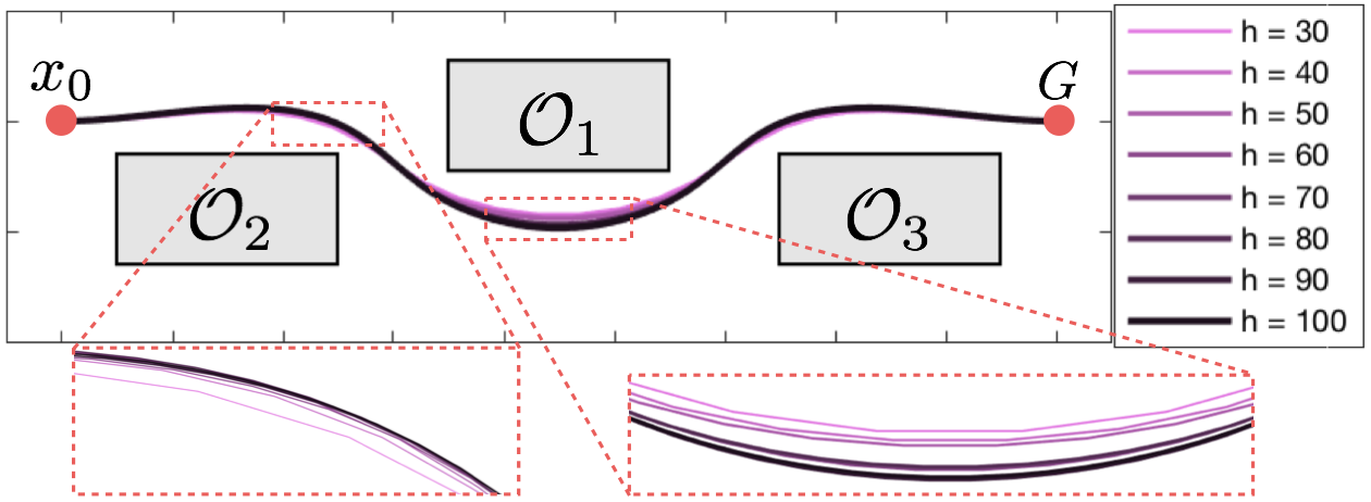
Figure 11: Scenario 1 and the optimal trajectories for different horizon $h$.

Table 1: Comparison among different algorithms.

		Scenario 1				Scenario 2
$h$	Method	Cost	Iter	Time	dT	Cost	Iter	Time	dT
100 or 60	SQP-M	1358.9	239	140.5s	-	5385.5	198	60.1s	-
	ITP-M	1358.9	470	50.6s	-	5349.6	320	18.0s	56.3ms
	CFS-M	1358.9	18	1.8s	98.8ms	5413.2	6	344.9ms	57.5ms
	SQP-C	1347.6	123	47.3s	-	5489.6	52	10.2s	-
	ITP-C	1341.7	306	2.9s	9.5ms	5349.6	123	595.0ms	4.8ms
	CFS-C	1358.9	18	74.4ms	4.1ms	5413.2	6	27.3ms	4.6ms
50	SQP-M	2299.5	110	25.8s	-	5539.6	164	40.0s	-
	ITP-M	1308.3	187	8.8s	47.1ms	5372.8	268	11.3s	42.2ms
	CFS-M	1458.2	8	212.1ms	26.5ms	5394.2	5	186.1s	37.2ms
	SQP-C	1308.3	52	3.4s	65.4ms	5682.0	62	5.7s	91.9ms
	ITP-C	1275.1	131	390ms	3.0ms	5555.8	96	495.6ms	5.2ms
	CFS-C	1458.2	8	23.7ms	3.0ms	5394.2	5	21.0ms	4.2ms
40	SQP-M	3391.6	97	15.6s	-	5318.1	127	23.2s	-
	ITP-M	1317.0	150	5.2s	34.7ms	5549.8	156	5.6s	35.9ms
	CFS-M	1317.0	8	172.6ms	21.6ms	5399.2	6	171.9	28.7ms
	SQP-C	1317.0	40	1.5s	37.5ms	5568.8	69	2.8s	40.6ms
	ITP-C	1170.5	102	240.5ms	2.4ms	5399.2	91	290.4ms	3.2ms
	CFS-C	1317.0	8	16.5ms	2.1ms	5399.2	6	19.0ms	3.2ms
30	SQP-M	1039.2	106	8.4s	79.2ms	5075.8	90	11.0s	-
	ITP-M	1039.2	109	2.8s	25.7ms	5162.4	127	3.2s	25.2ms
	CFS-M	1039.2	12	208.2ms	17.3ms	5167.3	5	110.6ms	22.1ms
	SQP-C	1453.3	27	379.1ms	14.0ms	5444.3	42	1.5s	35.7ms
	ITP-C	1039.2	59	118.5ms	2.0ms	5320.8	67	125.5ms	1.9ms
	CFS-C	1039.2	12	19.0ms	1.6ms	5167.3	5	12.2ms	2.4ms

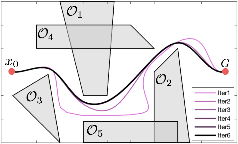
(a) Trajectories in CFS-C.

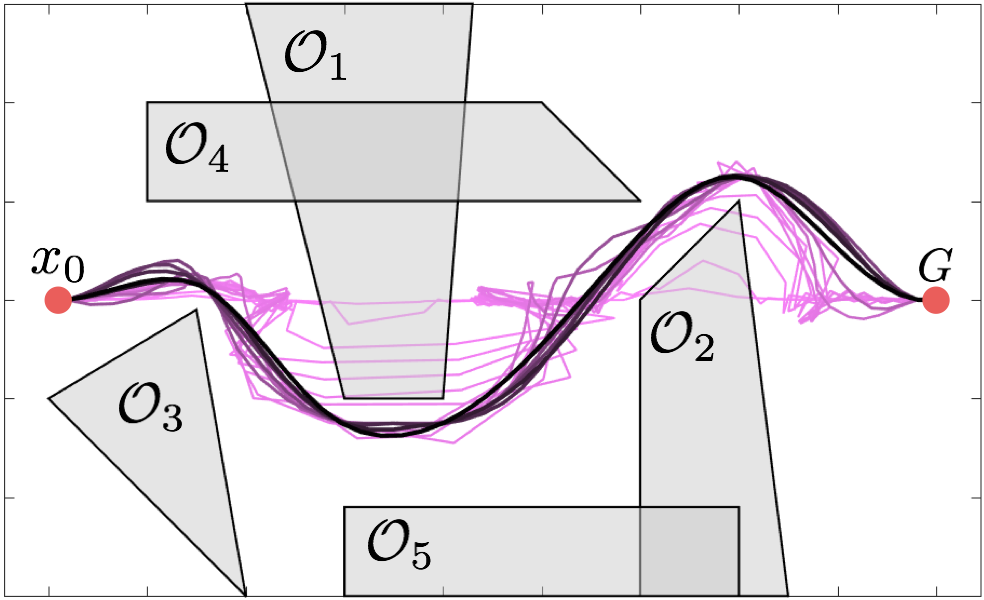
(b) Trajectories in ITP-C.

Figure 12: Scenario 2 and the trajectories before convergence for $h=50$.

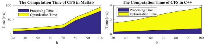
Figure 13: The decomposed time per iteration using Algorithm 1 in scenario 1.

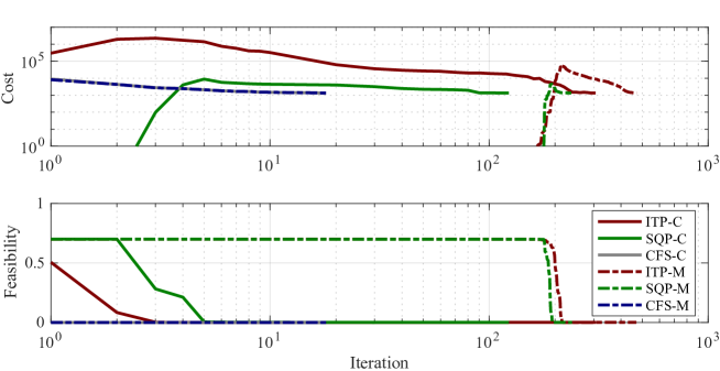
Figure 14: The run time statistics in scenario 1.

6 Conclusion

This paper introduced a fast algorithm for real time motion planning based on the convex feasible set. The CFS algorithm can handle problems that have convex cost function and non-convex constraints which are usually encountered in robot motion planning. By computing a convex feasible set within the non-convex constraints, the non-convex optimization problem is transformed into a convex optimization. Then by iteration, we can efficiently eliminate the error introduced by the convexification. It is proved in the paper that the proposed algorithm is feasible and stable. Moreover, it can converge to a local optimum if either the initial reference satisfies certain conditions or the constraints satisfy certain conditions. The performance of CFS is compared to that of ITP and SQP. It is shown that CFS reaches local optima faster than ITP and SQP, hence better suited for real time applications. In the future, methods for computing the convex feasible sets for infeasible references in complicated environments will be explored.

References

- [1] Optimization toolbox, constrained optimization, fmincon, https://www.mathworks.com/help/optim/ug/fmincon.html.
- [2] Every convex function is locally lipschitz, The American Mathematical Monthly, 79 (1972), pp. 1121–1124.
- [3] B. Açıkmeşe, J. M. Carson, and L. Blackmore, Lossless convexification of nonconvex control bound and pointing constraints of the soft landing optimal control problem, IEEE Transactions on Control Systems Technology, 21 (2013), pp. 2104–2113.
- [4] R. H. Byrd, J. Nocedal, and R. A. Waltz, Knitro: An Integrated Package for Nonlinear Optimization, Springer US, Boston, MA, 2006, pp. 35–59.
- [5] C. Chen, M. Rickert, and A. Knoll, Path planning with orientation-aware space exploration guided heuristic search for autonomous parking and maneuvering, in IEEE Intelligent Vehicles Symposium (IV), 2015, pp. 1148–1153.
- [6] F. H. Clarke, Generalized gradients and applications, Transactions of the American Mathematical Society, 205 (1975), pp. 247–262.
- [7] A. Colesanti and D. Hug, Hessian measures of semi-convex functions and applications to support measures of convex bodies, manuscripta mathematica, 101 (2000), pp. 209–238.
- [8] G. Eichfelder and J. Povh, On the set-semidefinite representation of nonconvex quadratic programs over arbitrary feasible sets, Optimization Letters, 7 (2013), pp. 1373–1386.
- [9] G. B. Folland, Real analysis: modern techniques and their applications, John Wiley & Sons, 2013.
- [10] E. Frazzoli, M. A. Dahleh, and E. Feron, Real-time motion planning for agile autonomous vehicles, Journal of Guidance, Control, and Dynamics, 25 (2002), pp. 116–129.
- [11] M. W. Harris and B. Açıkmeşe, Lossless convexification of non-convex optimal control problems for state constrained linear systems, Automatica, 50 (2014), pp. 2304–2311.
- [12] T. M. Howard, C. J. Green, and A. Kelly, Receding horizon model-predictive control for mobile robot navigation of intricate paths, in Field and Service Robotics, Springer, 2010, pp. 69–78.
- [13] T. A. Johansen, T. I. Fossen, and S. P. Berge, Constrained nonlinear control allocation with singularity avoidance using sequential quadratic programming, IEEE Transactions on Control Systems Technology, 12 (2004), pp. 211–216.
- [14] Y. Kuwata, J. Teo, G. Fiore, S. Karaman, E. Frazzoli, and J. P. How, Real-time motion planning with applications to autonomous urban driving, IEEE Transactions on Control Systems Technology, 17 (2009), pp. 1105–1118.
- [15] J.-C. Latombe, Robot motion planning, vol. 124, Springer Science & Business Media, 2012.
- [16] C. Liu, C.-Y. Lin, Y. Wang, and M. Tomizuka, Convex feasible set algorithm for constrained trajectory smoothing, in American Control Conference (ACC), IEEE, 2017, pp. 4177–4182.
- [17] C. Liu and M. Tomizuka, Algorithmic safety measures for intelligent industrial co-robots, in International Conference on Robotics and Automation (ICRA), IEEE, 2016, pp. 3095–3102.
- [18] C. Liu and M. Tomizuka, Enabling safe freeway driving for automated vehicles, in American Control Conference (ACC), IEEE, 2016, pp. 3461–3467.
- [19] C. Liu and M. Tomizuka, Real time trajectory optimization for nonlinear robotic systems: Relaxation and convexification, System & Control Letters, 108 (2017), pp. 56 – 63.
- [20] X. Liu, Autonomous trajectory planning by convex optimization, PhD thesis, Iowa State University, 2013.
- [21] X. Liu and P. Lu, Solving nonconvex optimal control problems by convex optimization, Journal of Guidance, Control, and Dynamics, (2014).
- [22] A. Matveev, M. Hoy, and A. Savkin, A method for reactive navigation of nonholonomic under-actuated robots in maze-like environments, Automatica, 49 (2013), pp. 1268 – 1274.
- [23] J. Nocedal and S. Wright, Numerical optimization, Springer Science & Business Media, 2006.
- [24] N. Ratliff, M. Zucker, J. A. Bagnell, and S. Srinivasa, CHOMP: Gradient optimization techniques for efficient motion planning, in International Conference on Robotics and Automation (ICRA), IEEE, 2009, pp. 489–494.
- [25] A. V. Savkin, A. S. Matveev, M. Hoy, and C. Wang, Safe Robot Navigation Among Moving and Steady Obstacles, Butterworth-Heinemann, 2015.
- [26] J. Schulman, J. Ho, A. X. Lee, I. Awwal, H. Bradlow, and P. Abbeel, Finding locally optimal, collision-free trajectories with sequential convex optimization., in Robotics: science and systems, vol. 9, Citeseer, 2013, pp. 1–10.
- [27] P. Spellucci, A new technique for inconsistent QP problems in the SQP method, Mathematical Methods of Operations Research, 47 (1998), pp. 355–400.
- [28] R. G. Strongin and Y. D. Sergeyev, Global optimization with non-convex constraints: Sequential and parallel algorithms, vol. 45, Springer Science & Business Media, 2013.
- [29] M. Tawarmalani and N. V. Sahinidis, Convexification and global optimization in continuous and mixed-integer nonlinear programming: theory, algorithms, software, and applications, vol. 65, Springer Science & Business Media, 2002.
- [30] K. Tone, Revisions of constraint approximations in the successive QP method for nonlinear programming problems, Mathematical Programming, 26 (1983), pp. 144–152.
- [31] J. Van Den Berg, P. Abbeel, and K. Goldberg, LQG-MP: Optimized path planning for robots with motion uncertainty and imperfect state information, The International Journal of Robotics Research, 30 (2011), pp. 895–913.
- [32] R. J. Vanderbei and D. F. Shanno, An interior-point algorithm for nonconvex nonlinear programming, Computational Optimization and Applications, 13 (1999), pp. 231–252.
- [33] Z. Zhu, E. Schmerling, and M. Pavone, A convex optimization approach to smooth trajectories for motion planning with car-like robots, in IEEE Conference on Decision and Control (CDC), IEEE, 2015, pp. 835–842.