On a randomized backward Euler method for
nonlinear evolution equations with
time-irregular coefficients

Abstract.

In this paper we introduce a randomized version of the backward Euler method, that is applicable to stiff ordinary differential equations and nonlinear evolution equations with time-irregular coefficients. In the finite-dimensional case, we consider Carathéodory type functions satisfying a one-sided Lipschitz condition. After investigating the well-posedness and the stability properties of the randomized scheme, we prove the convergence to the exact solution with a rate of $0.5$ in the root-mean-square norm assuming only that the coefficient function is square integrable with respect to the temporal parameter.

These results are then extended to the numerical solution of infinite-dimensional evolution equations under monotonicity and Lipschitz conditions. Here we consider a combination of the randomized backward Euler scheme with a Galerkin finite element method. We obtain error estimates that correspond to the regularity of the exact solution. The practicability of the randomized scheme is also illustrated through several numerical experiments.

1. Introduction

The aim of this paper is to introduce a new numerical scheme to approximate the solution of an ordinary differential equation (ODE) of Carathéodory type

(1.1) $$\begin{split}\begin{cases}\dot{u}(t)=f(t,u(t)),\quad\text{ for almost all }t\in(0,T],\\ u(0)=u_{0},\end{cases}\end{split}$$

for $T\in(0,\infty)$, and of a non-autonomous evolution equation

(1.2) $$\begin{split}\begin{cases}\dot{u}(t)+{\mathcal{A}}(t)u(t)=f(t),\quad\text{for almost all }t\in(0,T],\\ u(0)=u_{0},\end{cases}\end{split}$$

where ${\mathcal{A}}\colon[0,T]\times V\to V^{\ast}$ is a strongly monotone and Lipschitz continuous operator with respect to the second argument that is defined on a Gelfand triple $V\hookrightarrow H\cong H^{\ast}\hookrightarrow V^{\ast}$ for real Hilbert spaces $V$ and $H$.

We focus on the particular difficulty that the mappings $f$ and ${\mathcal{A}}$ are irregular with respect to the temporal parameter. More precisely, we do not impose any continuity conditions but only certain integrability requirements with respect to $t$. For a concise description of the general settings we refer to Sections 3 and 6, respectively. In particular, a precise statement of all conditions is given in Assumption 3.1 for (1.1) and in Assumption 6.1 for (1.2). To develop the idea of our scheme we mostly focus on the ODE problem (1.1) in this introduction. The derivation of the numerical scheme for the evolution equation (1.2) follows analogously and will be introduced in detail in Section 6.

When considering a right-hand side $f$ that is only integrable, every deterministic algorithm can be ”fooled” if it only uses information provided by point evaluations on prescribed (deterministic) points. One can easily construct suitable fooling functions for general classes of deterministic algorithms, for instance, based on adaptive strategies. In Sections 5 and 8 we give examples of such fooling functions and investigate the numerical behavior. Further, we refer to the vast literature on the information-based complexity theory (IBC), which applies similar techniques to derive lower bounds for the error of certain classes of deterministic and randomized numerical algorithms. For instance, see [34, 40] for a general introduction into IBC and [24, 27, 28] for applications to the numerical solution of initial value problems.

One way to construct numerical methods for the solution of initial value problems with time-irregular coefficients consists of allowing the algorithm to use additional information of the right-hand side $f$ as, for example, integrals of the form

(1.3) $$f^{n}(x):=\frac{1}{t_{n}-t_{n-1}}\int_{t_{n-1}}^{t_{n}}f(s,x)\,\mathrm{d}s,\quad\text{for }x\in{\mathbf{R}}^{d}.$$

This approach is often found in the existence theory of ODEs and PDEs when a numerical method is used to construct analytical solutions to the initial value problems (1.1) and (1.2) under minimal regularity assumptions. The complexity of such methods has also been studied in [27] (and the references therein) for the numerical solution of ODEs. It is also the state-of-the-art method in many recent papers for the numerical solution of evolution equations of the form (1.2). For example, we refer to [5, 15, 25, 33].

However, it is rarely discussed how a quantity such as $f^{n}(x)$ in (1.3) is obtained in practice. Strictly speaking, since the computation of $f^{n}(x)$ often requires the application of further numerical methods such as quadrature rules, algorithms relying on integrals such as (1.3) are, in general, not fully discrete solvers yet. More importantly, classical quadrature rules for the approximation of $f^{n}(x)$ are again based on deterministic point evaluations of $f$ and may therefore be “fooled”.

Instead of using linear functionals such as (1.3) we propose the following randomized version of the backward Euler method. For $N\in{\mathbf{N}}$, a step size $k=\frac{T}{N}$, and a temporal grid $0=t_{0}<t_{1}<\dots<t_{N}=T$ with $t_{n}=nk$ for $n\in\{0,\dots,N\}$, the randomized scheme for the numerical solution (1.1) is then given by

(1.4) $$\begin{split}\begin{cases}U^{n}=U^{n-1}+kf(\xi_{n},U^{n}),\quad\text{ for }n\in\{1,\ldots,N\},\\ U^{0}=u_{0},\end{cases}\end{split}$$

where $\xi_{n}$ is a uniformly distributed random variable with values in the interval $[t_{n-1},t_{n}]$. Note that we evaluate the right-hand side at random points between the grid points. Since the evaluation points vary every time the algorithm is called, it is not possible to construct a fooling function as described above.

We will prove in Theorem 4.7 that the numerical solution $U^{n}$ from (1.4) converges with (strong) order $\frac{1}{2}$ to the exact solution $u$ of (1.1), even if $f$ is only square integrable with respect to time. Due to the results in [24] this convergence rate is optimal in the sense that there exists no deterministic or randomized algorithm based on finitely many point evaluations of $f$ with a higher convergence rate within the class of all initial value problems satisfying Assumption 3.1.

The error analysis is based on the observation that the randomized scheme (1.4) is a hybrid of an implicit Runge–Kutta method and a Monte Carlo quadrature rule. In fact, if the ODE (1.1) is actually autonomous, that is, $f$ does not depend on $t$, then we recover the classical backward Euler method. On the other hand, if $f$ is independent of the state variable $u$, then the ODE (1.1) reduces to an integration problem and the randomized scheme (1.4) is the randomized Riemann sum for the approximation of $u_{0}+\int_{0}^{t_{n}}f(s)\,\mathrm{d}s$ given by

$$U^{n}=u_{0}+k\sum_{j=1}^{n}f(\xi_{j}),\quad\text{for }n\in\{1,\ldots,N\}.$$

Observe that a randomized Riemann sum is a particular case of stratified sampling from Monte Carlo integration. It was introduced in [19], [20] together with further, higher order, quadrature rules. Our error analysis of the randomized scheme (1.4) combines techniques for the analysis of both time-stepping schemes and Monte Carlo integration. In particular, since we are interested in the discretization of evolution equations in later sections, we apply techniques for the numerical analysis of stiff ODEs developed in [22] and for stochastic ODEs in [3].

Before we give a more detailed account of the remainder of this paper, let us emphasize a few practical advantages of the randomized scheme (1.4):

1. The implementation of the randomized scheme (1.4) is as difficult as for the classical backward Euler method in terms of the requirements of solving a nonlinear system of equations. On the other hand, the scheme (1.4) does not require integrals such as $f^{n}(x)$ if the right-hand side is time-irregular.

2. The same is true for the computational effort. Compared to the classical backward Euler method, the randomized scheme (1.4) only requires in each step the additional simulation of a single scalar-valued random variable. In general, the resulting additional computational effort is negligible compared to the solution of a potentially high-dimensional nonlinear system of equations. More importantly, due to the randomization we avoid the potentially costly computation of the integrals $f^{n}(x)$.

3. In contrast to every deterministic method based on point evaluations of $f$, the randomized scheme (1.4) is independent of the particular representation of an integrable function. To be more precise, let $g_{1}$ and $g_{2}$ be two representations of the same equivalence class $g\in L^{2}(0,T)$. Then, it follows that $g_{1}(\xi_{n})=g_{2}(\xi_{n})$ with probability one, since $g_{1}=g_{2}$ almost everywhere.

We remark that the last item is only valid as long as the random variable $\xi_{n}$ is indeed uniformly distributed in $[t_{n-1},t_{n}]$. In practice, however, one usually applies a pseudo-random number generator which only draws values from the set of floating point numbers. Since this is a null set with respect to the Lebesgue measure, the argument given above is no longer valid. Of course, this problem affects any algorithm that uses the floating point arithmetic. Nevertheless, a randomized algorithm is often more robust regarding the particular choice of the representation of an equivalence class in $L^{2}(0,T)$ and, hence, more user-friendly. For instance, the mapping $(0,T)\ni t\mapsto(T-t)^{-\frac{1}{3}}$ causes problems for the classical backward Euler method as it will evaluate the mapping in the singularity at $t=T$. This problem does not occur for the randomized backward Euler method with probability one.

Let us also mention that randomized algorithms for the numerical solution of initial value problems have already been studied in the literature. In the ODE case, the complexity and optimality of such algorithms is considered in [12, 24, 28] under various degrees of smoothness of $f$. The time-irregular case studied in the present paper was first investigated in [38, 39]. See also [26, 30] for a more recent exposition of explicit randomized schemes.

The present paper extends the earlier results in several directions. In order to deal with possibly stiff ODEs we consider a randomized version of the backward Euler method and prove its well-posedness and stability under a one-sided Lipschitz condition. In addition, we require only local Lipschitz conditions with respect to the state variable in order to obtain estimates on the local truncation error, thereby extending results from [30]. We also avoid any (local) boundedness condition on $f$ as, for example, in [12, 26].

The stability properties also qualify the randomized backward Euler method as a suitable temporal integrator for non-autonomous evolution equations with time-irregular coefficients. To the best of our knowledge, there is no work found in the literature that applies a randomized algorithm to the numerical solution of evolution equations of the form (1.2). Instead, the standard approach in the time-irregular case relies on the availability of suitable integrals of the right-hand side as in (1.3). In particular, we mention [15, 25]. Further results on optimal rates under minimal regularity assumptions for linear parabolic PDEs can be found, e.g., in [5, 9, 21]. For semilinear parabolic problems optimal error estimates are also found in [33], where a discontinuous Galerkin method in time and space is considered.

This paper is organized as follows. In Section 2, we shortly introduce the notation and recapture some important concepts of stochastic analysis that are relevant for this paper. In the following Section 3, we state the assumptions imposed on the ODE (1.1). We also discuss existence and regularity of the solution. In Section 4, we then prove the well-posedness and convergence of the randomized backward Euler method in the root-mean-square sense. The ODE part of this paper is completed in Section 5 by examining a numerical example.

In Section 6, we introduce the setting for the irregular non-autonomous evolution equation (1.2) that we consider in the second part of this paper. Under some additional regularity assumptions on the exact solution, we prove the convergence of a fully discrete method that combines the randomized backward Euler scheme with a Galerkin finite element method. The additional regularity assumption is then discussed in more detail in Section 7. In particular, it is shown that the regularity condition is fulfilled for rather general classes of linear and semilinear parabolic PDEs. Finally in Section 8, we demonstrate that this new randomized method can be applied to evolution equations. To this end, we present a numerical example which is based on the finite element software package FEniCS [31].

2. Preliminaries

In this section, we explain the necessary tools from probability theory and recall some important inequalities that are needed. First, we start by fixing the notation used in this paper.

We denote the set of all positive integers by ${\mathbf{N}}$ and the set of all real numbers by ${\mathbf{R}}$. In ${\mathbf{R}}^{d}$, $d\geq 1$, we denote the Euclidean norm by $|\cdot|$ which coincides with the absolute value of a real number for $d=1$. The standard inner product in ${\mathbf{R}}^{d}$ is denoted by $(\cdot,\cdot)$. For a ball of radius $r$ with center $x\in{\mathbf{R}}^{d}$ we write $B_{r}(x)\subseteq{\mathbf{R}}^{d}$.

In the following, we will consider different spaces of functions with values in general Hilbert spaces. To this end, let $(H,(\cdot,\cdot)_{H},\|\cdot\|_{H})$ be a real Hilbert space and $T>0$. We will denote the space of continuous functions on $[0,T]$ with values in $H$ by $C([0,T];H)$ where the norm is given by

$$\|f\|_{C([0,T];H)}=\sup_{t\in[0,T]}\|f(t)\|_{H}.$$

It will also be important to consider functions which are a little more regular. For $0<\gamma<1$ we denote the space of Hölder continuous functions by $C^{\gamma}([0,T];H)$ with norm given by

$$\|f\|_{C^{\gamma}([0,T];H)}=\sup_{t\in[0,T]}\|f(t)\|_{H}+\sup_{\begin{subarray}{c}s,t\in[0,T]\\ s\neq t\end{subarray}}\frac{\|f(s)-f(t)\|_{H}}{|s-t|^{\gamma}}.$$

For $p\in[1,\infty)$, we introduce the Bochner–Lebesgue space

$$L^{p}(0,T;H)=\left\{u:[0,T]\to H\,:\,u\text{ is strongly measurable and }\|u\|_{L^{p}(0,T;H)}<\infty\right\}$$

where the norm is given by

$$\|u\|_{L^{p}(0,T;H)}^{p}=\int_{0}^{T}\|u(t)\|_{H}^{p}\,\mathrm{d}t.$$

In the case $H={\mathbf{R}}$ we write $L^{p}(0,T)$.

The space of linear bounded operators from $H$ to a Banach space $(U,\|\cdot\|_{U})$ is denoted by ${\mathcal{L}}(H,U)$ and in the case of $U=H$ we write ${\mathcal{L}}(H)$. The norm of this space is the usual operator norm given by

$$\|A\|_{{\mathcal{L}}(H,U)}=\sup_{v\in H,\|v\|_{H}=1}\|Av\|_{U}.$$

Since we are interested in a randomized scheme, we will briefly recall the most important probabilistic concepts needed in this paper. To this end, we consider a probability space $(\Omega,{\mathcal{F}},{\mathbf{P}})$ which consists of a measurable space $(\Omega,{\mathcal{F}})$ together with a finite measure ${\mathbf{P}}$ such that ${\mathbf{P}}(A)\in[0,1]$ for every $A\in{\mathcal{F}}$ and ${\mathbf{P}}(\Omega)=1$. A mapping $X\colon\Omega\to H$ is called a random variable if it is measurable with respect to the $\sigma$-algebra ${\mathcal{F}}$ and the Borel $\sigma$-algebra ${\mathcal{B}}(H)$ in $H$, i.e., for every $B\in{\mathcal{B}}(H)$

$$X^{-1}(B)=\{\omega\in\Omega\,:\,X(\omega)\in B\}$$

is an element of ${\mathcal{F}}$. The integral of a random variable $X$ with respect to the measure ${\mathbf{P}}$ is often denoted by

$${\mathbf{E}}[X]=\int_{\Omega}X(\omega)\,\mathrm{d}{\mathbf{P}}(\omega).$$

The space of ${\mathcal{F}}$-measurable random variables $X$ such that ${\mathbf{E}}[\|X\|_{H}]$ is finite is denoted by $L^{1}(\Omega,{\mathcal{F}},{\mathbf{P}};H)$.

For our purposes it is important to consider the space $L^{2}(\Omega,{\mathcal{F}},{\mathbf{P}};H)$ of square integrable ${\mathcal{F}}$-measurable random variables. This space is often abbreviated by $L^{2}(\Omega;H)$ if it is clear from the context which $\sigma$-algebra ${\mathcal{F}}$ and measure ${\mathbf{P}}$ is used. The space is endowed with the norm

$$\|X\|^{2}_{L^{2}(\Omega;H)}=\int_{\Omega}\|X(\omega)\|_{H}^{2}\,\mathrm{d}{\mathbf{P}}(\omega)={\mathbf{E}}[\|X\|_{H}^{2}],\quad X\in L^{2}(\Omega;H).$$

Equipped with this norm and inner product

$$(X_{1},X_{2})_{L^{2}(\Omega;H)}=\int_{\Omega}(X_{1}(\omega),X_{2}(\omega))_{H}\,\mathrm{d}{\mathbf{P}}(\omega),\quad X_{1},X_{2}\in L^{2}(\Omega;H),$$

the space $L^{2}(\Omega;H)$ is a Hilbert space.

A further important concept is the independence of events $(A_{n})_{n\in{\mathbf{N}}}\subset{\mathcal{F}}$. We call the events $(A_{n})_{n\in{\mathbf{N}}}$ independent if for every finite subset $I\subset{\mathbf{N}}$

$${\mathbf{P}}\Big{(}\bigcap_{n\in I}A_{n}\Big{)}=\prod_{n\in I}{\mathbf{P}}(A_{n})$$

holds. This concept can be transferred to families $({\mathcal{F}}_{n})_{n\in{\mathbf{N}}}$ of $\sigma$-algebras. Such a family is called independent if for every finite subset $I\subset{\mathbf{N}}$ it follows that every choice of events $(A_{n})_{n\in I}$ with $A_{n}\in{\mathcal{F}}_{n}$ are independent. Similarly, a family of $H$-valued random variables $(X_{n})_{n\in{\mathbf{N}}}$ is called independent if the generated $\sigma$-algebras

$$\sigma(X_{n})=\{X_{n}^{-1}(B)\,:\,B\in{\mathcal{B}}(H)\}$$

are independent.

A family $({\mathcal{F}}_{n})_{n\in{\mathbf{N}}}$ of $\sigma$-algebras is called a filtration if for every $n\in{\mathbf{N}}$ the $\sigma$-algebra ${\mathcal{F}}_{n}$ is a subset of ${\mathcal{F}}$ and ${\mathcal{F}}_{n}\subset{\mathcal{F}}_{m}$ holds for $n\leq m$. Thus a random variable $X$ can be measurable with respect to ${\mathcal{F}}_{m}$ but not with respect to ${\mathcal{F}}_{n}$ for $n<m$. In some of the arguments in this paper it will be important to project an ${\mathcal{F}}_{m}$-measurable random variable to a smaller $\sigma$-algebra ${\mathcal{F}}_{n}$. To this end, we introduce the conditional expectation of $X$ with respect to ${\mathcal{F}}_{n}$: For a random variable $X\in L^{1}(\Omega,{\mathcal{F}}_{m},{\mathbf{P}};H)$ we introduce the ${\mathcal{F}}_{n}$-measurable random variable ${\mathbf{E}}[X|{\mathcal{F}}_{n}]\colon\Omega\to H$ which fulfills

$${\mathbf{E}}[X\mathds{1}_{A}]={\mathbf{E}}[{\mathbf{E}}[X|{\mathcal{F}}_{n}]\mathds{1}_{A}]$$

for every $A\in{\mathcal{F}}_{m}$ where $\mathds{1}_{A}$ is the characteristic function with respect to $A$. The random variable ${\mathbf{E}}[X|{\mathcal{F}}_{n}]$ is uniquely determined by these postulations. An important property of the conditional expectation of $X\in L^{1}(\Omega,{\mathcal{F}},{\mathbf{P}};H)$ is the tower property which states that for two $\sigma$-algebras ${\mathcal{F}}_{n}$ and ${\mathcal{F}}_{m}$ of the filtration $({\mathcal{F}}_{n})_{n\in{\mathbf{N}}}$ with ${\mathcal{F}}_{n}\subseteq{\mathcal{F}}_{m}$ we obtain that

$${\mathbf{E}}[{\mathbf{E}}[X|{\mathcal{F}}_{n}]|{\mathcal{F}}_{m}]={\mathbf{E}}[{\mathbf{E}}[X|{\mathcal{F}}_{m}]|{\mathcal{F}}_{n}]={\mathbf{E}}[X|{\mathcal{F}}_{n}].$$

In particular, if $X$ is already measurable with respect to ${\mathcal{F}}_{n}$ then ${\mathbf{E}}[X|{\mathcal{F}}_{n}]=X$ holds. If $\sigma(X)$ is independent of ${\mathcal{F}}_{n}$ we obtain that ${\mathbf{E}}[X|{\mathcal{F}}_{n}]={\mathbf{E}}[X]$.

In the course of this paper, we will often use random variables which are uniformly distributed on a given temporal interval $(a,b)$. To denote such a random variable $\tau\colon\Omega\to{\mathbf{R}}$ we write $\tau\sim\mathcal{U}(a,b)$.

For a deeper insight of the probabilistic background, we refer the reader to [29].

The following inequalities will be helpful in order to give suitable a priori bounds for the solution of a differential equation and the solution of a numerical scheme.

Lemma 2.1 (Discrete Gronwall lemma).

Let $(u_{n})_{n\in{\mathbf{N}}}$ and $(b_{n})_{n\in{\mathbf{N}}}$ be two nonnegative sequences which satisfy, for given $a\in[0,\infty)$ and $N\in{\mathbf{N}}$, that

$$u_{n}\leq a+\sum_{j=1}^{n-1}b_{j}u_{j},\quad\text{for all }n\in\{1,\dots,N\}.$$

Then, it follows that

$$u_{n}\leq a\exp\Big{(}\sum_{j=1}^{n-1}b_{j}\Big{)},\quad\text{for all }n\in\{1,\dots,N\},$$

where we use the convention $\sum_{j=1}^{0}b_{j}=0$.

Lemma 2.2 (Gronwall lemma).

If $u,a\in C([0,T])$ are nonnegative functions which satisfy, for given $b\in[0,\infty)$, that

$$u(t)\leq a(t)+b\int_{0}^{t}u(s)\,\mathrm{d}s,\quad\text{for every }t\in[0,T],$$

then

$$u(t)\leq\mathrm{e}^{bt}\max_{s\in[0,t]}a(s),\quad\text{for every }t\in[0,T].$$

For a proof of the discrete Gronwall lemma, we refer the reader to [10]. A proof of Lemma 2.2 can be found in [23].

3. A Carathéodory type ODE under a one-sided Lipschitz condition

In this section, we introduce an initial value problem involving an ordinary differential equation with a non-autonomous vector field of Carathéodory type, that satisfies a one-sided Lipschitz condition. We give a precise statement of all conditions on the coefficient function in Assumption 3.1, which are sufficient to ensure the existence of a unique global solution. The same conditions will also be used for the error analysis of the randomized backward Euler method in Section 4. Further, we briefly investigate the temporal regularity of the solution $u$.

Let $T\in(0,\infty)$. We are interested in finding an absolutely continuous mapping $u\colon[0,T]\to{\mathbf{R}}^{d}$ that is a solution to the initial value problem

(3.1) $$\begin{split}\begin{cases}\dot{u}(t)=f(t,u(t)),\quad\text{for almost all }t\in(0,T],\\ u(0)=u_{0},\end{cases}\end{split}$$

where $u_{0}\in{\mathbf{R}}^{d}$ denotes the initial value. The following conditions on the right-hand side $f\colon[0,T]\times{\mathbf{R}}^{d}\to{\mathbf{R}}^{d}$ will ensure the existence of a unique global solution.

Assumption 3.1.

The mapping $f\colon[0,T]\times{\mathbf{R}}^{d}\to{\mathbf{R}}^{d}$ is measurable. Moreover, there exists a null set ${\mathcal{N}}_{f}\in{\mathcal{B}}([0,T])$ such that:

• There exists $\nu\in[0,\infty)$ such that

  $$\big{(}f(t,x)-f(t,y),x-y\big{)}\leq\nu|x-y|^{2},$$

  for all $x,y\in{\mathbf{R}}^{d}$ and $t\in[0,T]\setminus{\mathcal{N}}_{f}$.

• There exists a mapping $g\colon[0,T]\to[0,\infty)$ with $g\in L^{2}(0,T;{\mathbf{R}})$ such that

  $$|f(t,0)|\leq g(t),\quad\text{ for all }t\in[0,T]\setminus{\mathcal{N}}_{f}.$$

• For every compact set $K\subset{\mathbf{R}}^{d}$ there exists a mapping $L_{K}\colon[0,T]\to[0,\infty)$ with $L_{K}\in L^{2}(0,T;{\mathbf{R}})$ such that

  $$|f(t,x)-f(t,y)|\leq L_{K}(t)|x-y|$$

  for all $x,y\in K$ and $t\in[0,T]\setminus{\mathcal{N}}_{f}$.

First, we note that from Assumption 3.1 (i) and (ii) we immediately get

(3.2) $$\begin{split}\big{(}f(t,x),x\big{)}&=\big{(}f(t,x)-f(t,0),x-0\big{)}+\big{(}f(t,0),x\big{)}\\ &\leq\nu|x|^{2}+g(t)|x|\end{split}$$

for all $x\in{\mathbf{R}}^{d}$ and $t\in[0,T]\setminus{\mathcal{N}}_{f}$.

Moreover, it is well-known that Assumption 3.1 (ii) and (iii) are sufficient to ensure the existence of a unique local solution $u\colon[0,T_{0})\to{\mathbf{R}}^{d}$ to the initial value problem (3.1) with a local existence time $T_{0}\leq T$, see for instance [23, Chap. I, Thm 5.3]. Here, we recall that a mapping $u\colon[0,T_{0})\to{\mathbf{R}}^{d}$ is a (local) solution in the sense of Carathéodory to (3.1) if $u$ is absolutely continuous and satisfies

(3.3) $$u(t)=u_{0}+\int_{0}^{t}f(s,u(s))\,\mathrm{d}s$$

for all $t\in[0,T_{0})$. Moreover, for almost all $t\in[0,T_{0})$ with $|u(t)|>0$ we have

$$|u(t)|\frac{\,\mathrm{d}missing}{\,\mathrm{d}t}|u(t)|=\frac{1}{2}\frac{\,\mathrm{d}missing}{\,\mathrm{d}t}|u(t)|^{2}=\big{(}f(t,u(t)),u(t)\big{)}\leq\nu|u(t)|^{2}+g(t)|u(t)|,$$

due to (3.2). Hence, by canceling $|u(t)|>0$ from both sides of the inequality we obtain

$$\frac{\,\mathrm{d}missing}{\,\mathrm{d}t}|u(t)|\leq\nu|u(t)|+g(t)$$

for almost all $t\in[0,T_{0})$ with $|u(t)|>0$. After integrating this inequality from $0$ to $t$ it follows

$$|u(t)|\leq|u_{0}|+\int_{0}^{t}g(s)\,\mathrm{d}s+\int_{0}^{t}\nu|u(s)|\,\mathrm{d}s,$$

which holds for all $t\in[0,T_{0})$. An application of the Gronwall lemma (Lemma 2.2) yields

(3.4) $$|u(t)|\leq\mathrm{e}^{\nu t}\Big{(}|u_{0}|+\int_{0}^{t}g(s)\,\mathrm{d}s\Big{)}$$

for all $t\in[0,T_{0})$. In particular, since $g\in L^{2}(0,T;{\mathbf{R}})$ we deduce from (3.4) that $u$ is in fact the unique global solution with $T_{0}=T$.

Finally, let us investigate the regularity of the solution $u$. To this end, we define

(3.5) $$K_{u}:=\Big{\{}x\in{\mathbf{R}}^{d}\,:\,|x|\leq\mathrm{e}^{\nu T}\Big{(}|u_{0}|+\int_{0}^{T}g(s)\,\mathrm{d}s\Big{)}\Big{\}}.$$

Clearly, $K_{u}\subset{\mathbf{R}}^{d}$ is a compact set, that contains the origin and the complete curve $[0,T]\ni t\mapsto u(t)\in{\mathbf{R}}^{d}$ due to (3.4). Then, an application of Assumption 3.1 (iii) with $K=K_{u}$ yields

(3.6) $$|f(t,u(t))|\leq L_{K_{u}}(t)|u(t)|+|f(t,0)|\leq L_{K_{u}}(t)|u(t)|+g(t)$$

for all $t\in[0,T]\setminus{\mathcal{N}}_{f}$.

For arbitrary $s,t\in[0,T]$ with $s<t$ it follows from (3.3) that

$$|u(s)-u(t)|\leq\int_{s}^{t}|f(z,u(z))|\,\mathrm{d}z.$$

Furthermore, after inserting (3.6), we have

$$|u(s)-u(t)| \leq\int_{s}^{t}L_{K_{u}}(z)|u(z)|+g(z)\,\mathrm{d}z$$

$$\leq\Big{(}1+\sup_{z\in[0,T]}|u(z)|\Big{)}\int_{s}^{t}\big{(}L_{K_{u}}(z)+g(z)\big{)}\,\mathrm{d}z.$$

Then, an application of the Cauchy–Schwarz inequality yields

(3.7) $$|u(s)-u(t)| \leq\big{(}1+\|u\|_{C([0,T];{\mathbf{R}}^{d})}\big{)}\big{\|}L_{K_{u}}+g\big{\|}_{L^{2}(0,T;{\mathbf{R}})}|s-t|^{\frac{1}{2}}$$

for all $s,t\in[0,T]$. This proves that $u$ is Hölder continuous with exponent $\frac{1}{2}$.

4. Error analysis of the randomized backward Euler method

This section is devoted to the error analysis of the randomized backward Euler method. Our error analysis partly relies on variational methods developed in [15], that have recently been adapted to stochastic problems in [3].

In this section, we consider the following randomized version of the backward Euler method: Let $N\in{\mathbf{N}}$ denote the number of temporal steps and set $k=\frac{T}{N}$ as the temporal step size. For given $N$ and $k$ we obtain an equidistant partition of the interval $[0,T]$ given by $t_{n}:=kn$, $n\in\{0,\dots,N\}$. Further, let $\tau=(\tau_{n})_{n\in{\mathbf{N}}}$ be a family of independent and $\mathcal{U}(0,1)$-distributed random variables on a complete probability space $(\Omega,{\mathcal{F}},{\mathbf{P}})$ and let $\xi=(\xi_{n})_{n\in{\mathbf{N}}}$ be the family of random variables given by $\xi_{n}=t_{n}+k\tau_{n}$ for $n\in{\mathbf{N}}$. Then the numerical approximation $(U^{n})_{n\in\{0,\dots,N\}}$ of the solution $u$ is determined by the recursion

(4.1) $$\begin{split}\begin{cases}U^{n}=U^{n-1}+kf(\xi_{n},U^{n}),\quad\text{ for }n\in\{1,\ldots,N\},\\ U^{0}=u_{0}.\end{cases}\end{split}$$

When investigating the solvability of this implicit equation, the mild step size restriction $k\nu<1$ becomes necessary due to the implicit structure of the scheme. When considering a dissipative equation which is the case when $\nu\leq 0$ the restriction disappears. This case corresponds to the setting of the monotone operators in Section 6.

Note that (4.1) is an implicit Runge–Kutta method with one stage and a randomized node. More precisely, in each step we apply one member of the following family of implicit Runge–Kutta methods determined by the Butcher tableau

(4.2) $$\begin{split}\begin{array}[]{c|c}\theta&1\\ \hline\cr&1\end{array}\end{split}$$

where the value of the parameter $\theta\in[0,1]$ is determined by the random variable $\tau_{j}$ in the $j$-th step.

Further, the resulting sequence $(U^{n})_{n\in\{0,\ldots,N\}}$ consists of random variables, since we artificially inserted randomness into the numerical method. From a probabilistic point of view, $(U^{n})_{n\in\{0,\ldots,N\}}$ is in fact a discrete time stochastic process, that takes values in ${\mathbf{R}}^{d}$ and is adapted to the complete filtration $({\mathcal{F}}_{n})_{n\in{\mathbf{N}}}$. Here, ${\mathcal{F}}_{n}\subset{\mathcal{F}}$ is the smallest complete $\sigma$-algebra such that the subfamily $(\tau_{j})_{j\in\{1,\ldots,n\}}$ is measurable. Note that ${\mathcal{F}}_{n}\subset{\mathcal{F}}_{m}$, whenever $n\leq m$. More precisely,

(4.3) $$\begin{split}{\mathcal{F}}_{0}&:=\sigma\big{(}{\mathcal{N}}\in{\mathcal{F}}\;:\;{\mathbf{P}}({\mathcal{N}})=0\big{)},\\ {\mathcal{F}}_{n}&:=\sigma\big{(}\sigma(\tau_{j}\;:\;j\in\{1,\ldots,n\})\cup{\mathcal{F}}_{0}\big{)},\quad n\in{\mathbf{N}}.\end{split}$$

In particular, each ${\mathbf{P}}$-null set (and each subset of a ${\mathbf{P}}$-null set) is contained in every $\sigma$-algebra ${\mathcal{F}}_{n}$, $n\in{\mathbf{N}}_{0}$.

Next, let us introduce the following set $\mathcal{G}^{2}_{N}$ of square-integrable and adapted grid functions. For each $N\in{\mathbf{N}}$ this set is defined by

$$\mathcal{G}^{2}_{N}:=\big{\{} Z\colon\{0,\ldots,N\}\times\Omega\to{\mathbf{R}}^{d}\,:\,Z^{0}=z_{0}\in{\mathbf{R}}^{d},$$

$$Z^{n},f(\xi_{n},Z^{n})\in L^{2}(\Omega,{\mathcal{F}}_{n},{\mathbf{P}};{\mathbf{R}}^{d})\text{ for }n\in\{1,\ldots,N\}\big{\}}.$$

Take note that $z_{0}\in{\mathbf{R}}^{d}$ is an arbitrary deterministic initial value and that the condition $Z^{n}\in L^{2}(\Omega,{\mathcal{F}}_{n},{\mathbf{P}};{\mathbf{R}}^{d})$ ensures that $Z^{n}$ is square-integrable as well as measurable with respect to the $\sigma$-algebra ${\mathcal{F}}_{n}$. First, we will show that the randomized backward Euler method (4.1) with a sufficiently large number $N\in{\mathbf{N}}$ of steps uniquely determines an element in $\mathcal{G}^{2}_{N}$.

We begin by proving the existence of a solution to the implicit scheme. First, we state two technical lemmata to prove the existence and measurability of a solution.

Lemma 4.1.

For $R\in(0,\infty)$ let $h\colon\overline{B_{R}(0)}\subseteq{\mathbf{R}}^{d}\to{\mathbf{R}}^{d}$ be continuous and fulfill the condition

$$(h(x),x)\geq 0,\quad\text{ for every }x\in\partial B_{R}(0).$$

Then there exists at least one $x_{0}\in\overline{B_{R}(0)}$ such that $h(x_{0})=0$.

A proof of Lemma 4.1 is found, for instance, in [16, Sec. 9.1].

Remark 4.2.

For a symmetric, positive definite $Q\in{\mathbf{R}}^{d,d}$ Lemma 4.1 can be extended as follows. If a function $h\colon B_{Q,R}\subseteq{\mathbf{R}}^{d}\to{\mathbf{R}}^{d}$ where $B_{Q,R}$ is given by

$$B_{Q,R}=\{x\in{\mathbf{R}}^{d}\,:\,(Qx,x)\leq R^{2}\}$$

is continuous and fulfills

$$(Qh(x),x)\geq 0,\quad\text{ for every }x\in\partial B_{Q,R},$$

then there exists $x_{0}\in B_{Q,R}$ such that $h(x_{0})=0$. This extension of Lemma 4.1 can be proved by exploiting that

$$(Qh(x),x)\geq 0,\quad\text{ for every }x\in{\mathbf{R}}^{d}\text{ with }(Qx,x)=R^{2},$$

can be rewritten as

$$(Q^{\frac{1}{2}}h(Q^{-\frac{1}{2}}y),y)\geq 0,\quad\text{ for every }y\in{\mathbf{R}}^{d}\text{ with }(y,y)=R^{2},$$

using the transformation $y=Q^{\frac{1}{2}}x$.

The next result is needed in order to prove the measurability of the sequence generated by the implicit numerical method (4.1). For a closely related result we refer to [17, Lem. 3.8]. The proof presented here follows an approach from [13, Prop. 1], that can easily be extended to more general situations.

Lemma 4.3.

Let $\tilde{\mathcal{F}}$ be a complete sub $\sigma$-algebra of the $\sigma$-algebra ${\mathcal{F}}$, $\mathcal{M}\in\tilde{\mathcal{F}}$ with ${\mathbf{P}}(\mathcal{M})=1$ and $h\colon\Omega\times{\mathbf{R}}^{d}\to{\mathbf{R}}^{d}$ such that the following conditions are fulfilled.

1. The mapping $x\mapsto h(\omega,x)$ is continuous for every $\omega\in\mathcal{M}$.

2. The mapping $\omega\mapsto h(\omega,x)$ is $\tilde{\mathcal{F}}$-measurable for every $x\in{\mathbf{R}}^{d}$.

3. For every $\omega\in\mathcal{M}$ there exists a unique root of the function $h(\omega,\cdot)$.

Define the mapping

$$U\colon\Omega\to{\mathbf{R}}^{d},\quad\omega\mapsto U(\omega),$$

where $U(\omega)$ is the unique root of $h(\omega,\cdot)$ for $\omega\in\mathcal{M}$ and $U(\omega)$ is arbitrary for $\omega\in\Omega\setminus\mathcal{M}$. Then $U$ is $\tilde{\mathcal{F}}$-measurable.

Proof.

Define the (multivalued) mapping

$$U_{\varepsilon}\colon\Omega\to{\mathcal{P}}({\mathbf{R}}^{d}),\quad U_{\varepsilon}(\omega) :=\{x\in{\mathbf{R}}^{d}\,:\,h(\omega,x)\in B_{\varepsilon}(0)\}$$

for $\varepsilon>0$. We first show for an arbitrary open set $A\in{\mathcal{B}}({\mathbf{R}}^{d})$ that the set

$$U_{\varepsilon}^{-1}(A) :=\{\omega\in\Omega\,:\,\text{ there exists }x\in A\text{ such that }h(\omega,x)\in B_{\varepsilon}(0)\}$$

$$=\bigcup_{x\in A}\{\omega\in\Omega\,:\,h(\omega,x)\in B_{\varepsilon}(0)\}$$

is an element of $\tilde{\mathcal{F}}$. To this end, first note that $h(\cdot,x)^{-1}(B_{\varepsilon}(0))\in\tilde{\mathcal{F}}$ since $\omega\mapsto h(\omega,x)$ is $\tilde{\mathcal{F}}$-measurable. Then, it follows that

$$U_{\varepsilon}^{-1}(A\cap{\mathbf{Q}}^{d}) =\bigcup_{x\in A\cap{\mathbf{Q}}^{d}}\{\omega\in\Omega\,:\,h(\omega,x)\in B_{\varepsilon}(0)\}$$

$$=\bigcup_{x\in A\cap{\mathbf{Q}}^{d}}h(\cdot,x)^{-1}(B_{\varepsilon}(0))\in\tilde{\mathcal{F}}.$$

It remains to verify the equality

(4.4) $$U_{\varepsilon}^{-1}(A)=U_{\varepsilon}^{-1}(A\cap{\mathbf{Q}}^{d}).$$

It is clear that $U_{\varepsilon}^{-1}(A\cap{\mathbf{Q}}^{d})$ is a subset of $U_{\varepsilon}^{-1}(A)$.

To prove $U_{\varepsilon}^{-1}(A)\subseteq U_{\varepsilon}^{-1}(A\cap{\mathbf{Q}}^{d})$ we consider two cases. If $U_{\varepsilon}^{-1}(A)$ is a subset of $\Omega\setminus\mathcal{M}$ then it is a null set and lies in $\tilde{\mathcal{F}}$ due to the completeness of the $\sigma$-algebra. Else, we can assume that there exist $\omega\in U_{\varepsilon}^{-1}(A)\cap\mathcal{M}$ and $x_{0}\in A$ with $h(\omega,x_{0})\in B_{\varepsilon}(0)$. In particular, we note that the function $x\mapsto h(\omega,x)$ is continuous, since $\omega\in\mathcal{M}$. Further, observe that $A$ is an open neighborhood of $x_{0}$ and $B_{\varepsilon}(0)$ is an open neighborhood of $h(\omega,x_{0})$. Since $B_{\varepsilon}(0)$ is open, the continuity of $h$ implies that the set

$$C:=h(\omega,\cdot)^{-1}(B_{\varepsilon}(0))$$

is an open set in ${\mathbf{R}}^{d}$ with $x_{0}\in C$. Thus, $C\cap A$ is nonempty and open. Therefore, there exists $\overline{x}\in(C\cap A)\cap{\mathbf{Q}}^{d}$ such that $h(\omega,\overline{x})\in B_{\varepsilon}(0)$. This implies $\omega\in U_{\varepsilon}^{-1}(A\cap{\mathbf{Q}}^{d})$ and completes the proof of (4.4). Consequently, $U_{\varepsilon}^{-1}(A)\in\tilde{\mathcal{F}}$ for each open set $A\in{\mathcal{B}}({\mathbf{R}}^{d})$.

Next, recall that for each $\omega\in\mathcal{M}$ the image of $U$ is defined as the unique element of $h(\omega,\cdot)^{-1}(\{0\})$. Thus, the set

$$U_{0}(\omega):=\bigcap_{j\in{\mathbf{N}}}U_{\frac{1}{j}}(\omega)$$

consists of a single element which coincides with $U(\omega)$. Therefore we obtain

$$\mathcal{M}\cap U^{-1}(A) =\mathcal{M}\cap\{\omega\in\Omega:\text{ there exists }x\in A\text{ such that }h(\omega,x)=0\}$$

$$=\mathcal{M}\cap\bigcap_{j\in{\mathbf{N}}}\{\omega\in\Omega\,:\,\text{ there exists }x\in A\text{ such that }h(\omega,x)\in B_{\frac{1}{j}}(0)\}$$

$$=\mathcal{M}\cap\bigcap_{j\in{\mathbf{N}}}U_{\frac{1}{j}}^{-1}(A)=\mathcal{M}\cap\bigcap_{j\in{\mathbf{N}}}U_{\frac{1}{j}}^{-1}(A\cap{\mathbf{Q}}^{d})\in\tilde{\mathcal{F}},$$

which also implies $U^{-1}(A)\in\tilde{\mathcal{F}}$ for every open set $A\in{\mathcal{B}}({\mathbf{R}}^{d})$ due to the completeness of $\tilde{\mathcal{F}}$. From this the measurability of the mapping $\omega\mapsto U(\omega)$ follows. ∎

Lemma 4.4.

Let Assumption 3.1 be satisfied. Then for each $N\in{\mathbf{N}}$ with $\frac{T}{N}\nu=k\nu<1$ there exists a unique solution $U=(U^{n})_{n\in\{0,\dots,N\}}\in\mathcal{G}^{2}_{N}$ to the implicit scheme (4.1).

Proof.

The assertion $U^{n}\in L^{2}(\Omega,{\mathcal{F}}_{n},{\mathbf{P}};{\mathbf{R}}^{d})$ is proved using an inductive argument for $n\in\{0,\dots,N\}$. Since $U^{0}\equiv u_{0}\in L^{2}(\Omega,{\mathcal{F}}_{0},{\mathbf{P}};{\mathbf{R}}^{d})$ the case $n=0$ is evident. Next, assuming $U^{n-1}\in L^{2}(\Omega,{\mathcal{F}}_{n-1},{\mathbf{P}};{\mathbf{R}}^{d})$ exists, we define the set

$$\mathcal{M}=\{\omega\in\Omega\,:\,g(\xi_{n}(\omega))<\infty,\ |U^{n-1}(\omega)|<\infty\text{ and }\xi_{n}(\omega)\in[0,T]\setminus{\mathcal{N}}_{f}\},$$

where ${\mathcal{N}}_{f}\in{\mathcal{B}}([0,T])$ is the null set from Assumption 3.1. Since $\|g\|_{L^{2}(0,T;{\mathbf{R}})}<\infty$ and $\|U^{n-1}\|_{L^{2}(\Omega;{\mathbf{R}}^{d})}<\infty$ the set fulfills ${\mathbf{P}}(\mathcal{M})=1$. We define the function $h_{n}$ by

(4.5) $$h_{n}\colon\Omega\times{\mathbf{R}}^{d}\to{\mathbf{R}}^{d},\quad h_{n}(\omega,x)=x-U^{n-1}(\omega)-kf(\xi_{n}(\omega),x).$$

In the following we consider a fixed $\omega\in\mathcal{M}$. Then the mapping $h_{n}(\omega,\cdot)$ is continuous by Assumption 3.1 (iii). Further we write

$$R=R(\omega)=\frac{1}{1-\nu k}(|U^{n-1}(\omega)|+kg(\xi_{n}(\omega))).$$

Thus, for each $x\in{\mathbf{R}}^{d}$ with $|x|=R$ this implies

$$(h_{n}(\omega,x),x) =|x|^{2}-(U^{n-1}(\omega),x)-k(f(\xi_{n}(\omega),x),x)$$

$$\geq R^{2}-|U^{n-1}(\omega)|R-k\nu R^{2}-kg(\xi_{n}(\omega))R$$

$$=R^{2}-k\nu R^{2}-(|U^{n-1}(\omega)|+kg(\xi_{n}(\omega)))R$$

$$\geq(1-\nu k)R^{2}-(1-\nu k)R^{2}=0.$$

Hence, by Lemma 4.1, for every $\omega\in\mathcal{M}$ there exists $x=x(\omega)\in{\mathbf{R}}^{d}$ such that $h_{n}(\omega,x)=0$ holds. This $x$ is always unique: Assume there exists $\omega\in\mathcal{M}$ and $x,y\in{\mathbf{R}}^{d}$ such that

$$x=U^{n-1}(\omega)+kf(\xi_{n}(\omega),x)\quad\text{ and }\quad y=U^{n-1}(\omega)+kf(\xi_{n}(\omega),y)$$

hold. Then we can write for the difference

$$|x-y|^{2} =k\big{(}f(\xi_{n}(\omega),x)-f(\xi_{n}(\omega),y),x-y\big{)}$$

$$\leq k\nu|x-y|^{2}<|x-y|^{2}$$

which implies $x=y$. Thus, the function $h_{n}\colon\Omega\times{\mathbf{R}}^{d}\to{\mathbf{R}}^{d}$ is ${\mathcal{F}}_{n}$-measurable in the first entry, continuous in the second and has a unique root $x$ for every $\omega\in\mathcal{M}$. Then, Lemma 4.3 implies that the function

$$U^{n}\colon\Omega\to{\mathbf{R}}^{d},\quad\omega\mapsto U^{n}(\omega),$$

where $U^{n}(\omega)$ is the unique root of $h_{n}(\omega,\cdot)$ for $\omega\in\mathcal{M}$ and $U^{n-1}(\omega)$ for $\omega\in\Omega\setminus\mathcal{M}$ is ${\mathcal{F}}_{n}$-measurable.

It remains to prove that $U^{n}$ is finite with respect to the $L^{2}(\Omega;{\mathbf{R}}^{d})$-norm. Using (3.2), it follows

$$\|U^{n}\|_{L^{2}(\Omega;{\mathbf{R}}^{d})}^{2} ={\mathbf{E}}[(U^{n-1},U^{n})+k(f(\xi_{n},U^{n}),U^{n})]$$

$$\leq\|U^{n-1}\|_{L^{2}(\Omega;{\mathbf{R}}^{d})}\|U^{n}\|_{L^{2}(\Omega;{\mathbf{R}}^{d})}+k{\mathbf{E}}[\nu|U^{n}|^{2}+g(\xi_{n})|U^{n}|]$$

$$\leq\|U^{n-1}\|_{L^{2}(\Omega;{\mathbf{R}}^{d})}\|U^{n}\|_{L^{2}(\Omega;{\mathbf{R}}^{d})}+k\nu\|U^{n}\|^{2}_{L^{2}(\Omega;{\mathbf{R}}^{d})}$$

$$\quad+\sqrt{k}\|g\|_{L^{2}(0,T;{\mathbf{R}})}\|U^{n}\|_{L^{2}(\Omega;{\mathbf{R}}^{d})}$$

and therefore

$$\|U^{n}\|_{L^{2}(\Omega;{\mathbf{R}}^{d})} \leq\frac{1}{1-k\nu}\big{(}\|U^{n-1}\|_{L^{2}(\Omega;{\mathbf{R}}^{d})}+\sqrt{k}\|g\|_{L^{2}(0,T;{\mathbf{R}})}\big{)}.$$

The last step is to prove that the function $f(\xi_{n},U^{n})$ also lies in $L^{2}(\Omega,{\mathcal{F}}_{n},{\mathbf{P}};{\mathbf{R}}^{d})$. The mapping $\omega\mapsto f(\xi_{n}(\omega),U^{n}(\omega))$ is ${\mathcal{F}}_{n}$-measurable since $f$ is measurable and both $\xi_{n}$ and $U^{n}$ are ${\mathcal{F}}_{n}$-measurable. Since both $U^{n}$ and $U^{n-1}$ are elements of $L^{2}(\Omega;{\mathbf{R}}^{d})$ we can write

$$\|f(\xi_{n},U^{n})\|_{L^{2}(\Omega;{\mathbf{R}}^{d})}=\|\tfrac{1}{k}(U^{n}-U^{n-1})\|_{L^{2}(\Omega;{\mathbf{R}}^{d})}.$$

Thus, $f(\xi_{n},U^{n})$ is finite in the $L^{2}(\Omega;{\mathbf{R}}^{d})$-norm. ∎

The following stability lemma will play an important role in the error analysis of the randomized backward Euler method. Its proof is based on techniques developed in [3]. For its formulation we introduce the local residual $(\rho_{N}^{n}(V))_{n\in\{0,\ldots,N\}}$, $N\in{\mathbf{N}}$, of an arbitrary grid function $V=(V^{n})_{n\in\{0,\ldots,N\}}\in\mathcal{G}^{2}_{N}$. More precisely, for every $n\in\{1,\ldots,N\}$ we define $\rho_{N}^{n}(V)$ by

(4.6) $$\rho_{N}^{n}(V)=kf(\xi_{n},V^{n})-V^{n}+V^{n-1}.$$

Since $(V^{n})_{n\in\{0,\ldots,N\}}\in\mathcal{G}^{2}_{N}$ it directly follows that $\rho_{N}^{n}(V)\in L^{2}(\Omega,{\mathcal{F}}_{n},{\mathbf{P}};{\mathbf{R}}^{d})$ for every $n\in\{0,\ldots,N\}$.

Lemma 4.5.

Let Assumption 3.1 be satisfied. For $N\in{\mathbf{N}}$ let $(U^{n})_{n\in\{0,\ldots,N\}}\in\mathcal{G}^{2}_{N}$ be the grid function generated by (4.1) with step size $k=\frac{T}{N}$. If $\nu k<\frac{1}{4}$, then for every $V\in\mathcal{G}^{2}_{N}$ it holds true that

$$\big{\|}U^{n}-V^{n}\big{\|}_{L^{2}(\Omega;{\mathbf{R}}^{d})}$$

$$\leq\mathrm{e}^{(2\nu+1)t_{n}}\bigg{(} \big{|}U^{0}-V^{0}\big{|}^{2}$$

$$+\sum_{j=1}^{n}\Big{(}2\big{\|}\rho_{N}^{j}(V)\big{\|}^{2}_{L^{2}(\Omega;{\mathbf{R}}^{d})}+\frac{2}{k}\big{\|}{\mathbf{E}}[\rho_{N}^{j}(V)|{\mathcal{F}}_{j-1}]\big{\|}^{2}_{L^{2}(\Omega;{\mathbf{R}}^{d})}\Big{)}\bigg{)}^{\frac{1}{2}}$$

for every $n\in\{1,\ldots,N\}$.

Proof.

Let $N\in{\mathbf{N}}$ and $V=(V^{j})_{j\in\{0,\ldots,N\}}\in\mathcal{G}^{2}_{N}$ be arbitrary. Set $E^{j}:=U^{j}-V^{j}$ for each $j\in\{0,\ldots,N\}$. Since $(a-b,a)=\frac{1}{2}\big{(}|a|^{2}-|b|^{2}+|a-b|^{2}\big{)}$ for all $a,b\in{\mathbf{R}}^{d}$ we get for every $j\in\{1,\ldots,N\}$

$$|E^{j}|^{2}-|E^{j-1}|^{2}+|E^{j}-E^{j-1}|^{2}=2\big{(}E^{j}-E^{j-1},E^{j}\big{)}$$

$$\quad=2k\big{(}f(\xi_{j},U^{j})-f(\xi_{j},V^{j}),E^{j}\big{)}+2\big{(}kf(\xi_{j},V^{j})-V^{j}+V^{j-1},E^{j}\big{)}.$$

Next, note that ${\mathbf{P}}(\xi_{j}\in{\mathcal{N}}_{f})=0$, where ${\mathcal{N}}_{f}$ denotes the null set from Assumption 3.1. Hence, we can apply Assumption 3.1 (i) to the first term on a set with probability one. In addition, we insert (4.6) into the second term and obtain the inequality

$$|E^{j}|^{2}-|E^{j-1}|^{2}+|E^{j}-E^{j-1}|^{2}$$

$$\quad\leq 2\nu k|E^{j}|^{2}+2\big{(}\rho_{N}^{j}(V),E^{j}-E^{j-1}\big{)}+2\big{(}\rho_{N}^{j}(V),E^{j-1}\big{)}\quad\text{almost surely.}$$

After taking the expected value we further observe that

$${\mathbf{E}}\big{[}\big{(}\rho_{N}^{j}(V),E^{j-1}\big{)}\big{]} =\big{\langle}\rho_{N}^{j}(V),E^{j-1}\big{\rangle}_{L^{2}(\Omega;{\mathbf{R}}^{d})}=\big{\langle}{\mathbf{E}}[\rho_{N}^{j}(V)|{\mathcal{F}}_{j-1}],E^{j-1}\big{\rangle}_{L^{2}(\Omega;{\mathbf{R}}^{d})},$$

since $E^{j-1}$ is ${\mathcal{F}}_{j-1}$-measurable. Then, applications of the Cauchy–Schwarz inequality and the weighted Young inequality yield

$$2\big{\langle}{\mathbf{E}}[\rho_{N}^{j}(V)|{\mathcal{F}}_{j-1}],E^{j-1}\big{\rangle}_{L^{2}(\Omega;{\mathbf{R}}^{d})}$$

$$\quad\leq\frac{1}{k}\big{\|}{\mathbf{E}}[\rho_{N}^{j}(V)|{\mathcal{F}}_{j-1}]\big{\|}^{2}_{L^{2}(\Omega;{\mathbf{R}}^{d})}+k\big{\|}E^{j-1}\big{\|}^{2}_{L^{2}(\Omega;{\mathbf{R}}^{d})}.$$

In the same way, the Cauchy–Schwarz and Young inequalities also yield

$${\mathbf{E}}\big{[}2\big{(}\rho_{N}^{j}(V),E^{j}-E^{j-1}\big{)}\big{]}\leq\big{\|}\rho_{N}^{j}(V)\big{\|}^{2}_{L^{2}(\Omega;{\mathbf{R}}^{d})}+\big{\|}E^{j}-E^{j-1}\big{\|}^{2}_{L^{2}(\Omega;{\mathbf{R}}^{d})}.$$

Altogether, we have shown that

$$\|E^{j}\|^{2}_{L^{2}(\Omega;{\mathbf{R}}^{d})}-\|E^{j-1}\|^{2}_{L^{2}(\Omega;{\mathbf{R}}^{d})}$$

$$\quad\leq 2\nu k\|E^{j}\|^{2}_{L^{2}(\Omega;{\mathbf{R}}^{d})}+\big{\|}\rho_{N}^{j}(V)\big{\|}^{2}_{L^{2}(\Omega;{\mathbf{R}}^{d})}$$

$$\qquad+\frac{1}{k}\big{\|}{\mathbf{E}}[\rho_{N}^{j}(V)|{\mathcal{F}}_{j-1}]\big{\|}^{2}_{L^{2}(\Omega;{\mathbf{R}}^{d})}+k\big{\|}E^{j-1}\big{\|}^{2}_{L^{2}(\Omega;{\mathbf{R}}^{d})},$$

where we canceled the term $\|E^{j}-E^{j-1}\|^{2}_{L^{2}(\Omega;{\mathbf{R}}^{d})}$ on both sides of the inequality. Then, after some rearrangements and summing this inequality for all $j\in\{1,\ldots,n\}$ with arbitrary $n\in\{1,\ldots,N\}$ we obtain

$$(1-2\nu k)\|E^{n}\|^{2}_{L^{2}(\Omega;{\mathbf{R}}^{d})} \leq(1-2\nu k)\|E^{0}\|^{2}_{L^{2}(\Omega;{\mathbf{R}}^{d})}+(2\nu+1)k\sum_{j=1}^{n}\big{\|}E^{j-1}\big{\|}^{2}_{L^{2}(\Omega;{\mathbf{R}}^{d})}$$

$$\quad+\sum_{j=1}^{n}\Big{(}\big{\|}\rho_{N}^{j}(V)\big{\|}^{2}_{L^{2}(\Omega;{\mathbf{R}}^{d})}+\frac{1}{k}\big{\|}{\mathbf{E}}[\rho_{N}^{j}(V)|{\mathcal{F}}_{j-1}]\big{\|}^{2}_{L^{2}(\Omega;{\mathbf{R}}^{d})}\Big{)}.$$

Next, note that from the assumption $\nu k<\frac{1}{4}$ it follows $(1-2\nu k)^{-1}\leq 2$. Therefore,

$$\|E^{n}\|^{2}_{L^{2}(\Omega;{\mathbf{R}}^{d})} \leq\|E^{0}\|^{2}_{L^{2}(\Omega;{\mathbf{R}}^{d})}+2(2\nu+1)k\sum_{j=1}^{n}\big{\|}E^{j-1}\big{\|}^{2}_{L^{2}(\Omega;{\mathbf{R}}^{d})}$$

$$\quad+\sum_{j=1}^{n}\Big{(}2\big{\|}\rho_{N}^{j}(V)\big{\|}^{2}_{L^{2}(\Omega;{\mathbf{R}}^{d})}+\frac{2}{k}\big{\|}{\mathbf{E}}[\rho_{N}^{j}(V)|{\mathcal{F}}_{j-1}]\big{\|}^{2}_{L^{2}(\Omega;{\mathbf{R}}^{d})}\Big{)}.$$

Finally, applying a discrete Gronwall lemma (Lemma 2.1) completes the proof. ∎

The second ingredient in the error analysis is an estimate of the local residual of the exact solution. For its formulation we need to represent the exact solution by a grid function. This is easily achieved by restricting $u$ to the temporal points $t_{n}=nk$, $n\in\{0,\ldots,N\}$, with $k=\frac{T}{N}$ and $N\in{\mathbf{N}}$. More precisely, we define the restriction $u|_{N}$ of $u$ to the grid points $(t_{n})_{n\in\{0,\ldots,N\}}$ by

(4.7) $$[u|_{N}]^{n}:=u(t_{n})$$

for all $n\in\{0,\ldots,N\}$. Since $u|_{N}$ is deterministic we clearly have $[u|_{N}]^{n}=u(t_{n})\in L^{2}(\Omega,{\mathcal{F}}_{n},{\mathbf{P}};{\mathbf{R}}^{d})$ for all $n\in\{0,\ldots,N\}$. In addition, as in (3.6) we have

$$\|f(\xi_{n},u(t_{n}))\|_{L^{2}(\Omega;{\mathbf{R}}^{d})} \leq\big{\|}L_{K_{u}}(\xi_{n})|u(t_{n})|+g(\xi_{n})\big{\|}_{L^{2}(\Omega;{\mathbf{R}})}$$

$$\leq\frac{1}{\sqrt{k}}\big{(}1+\|u\|_{C([0,T];{\mathbf{R}}^{d})}\big{)}\big{\|}L_{K_{u}}+g\big{\|}_{L^{2}(t_{n-1},t_{n};{\mathbf{R}})}<\infty.$$

This shows that $u|_{N}\in\mathcal{G}^{2}_{N}$ for every $N\in{\mathbf{N}}$.

Lemma 4.6.

Let Assumption 3.1 be satisfied. Then, for all $N\in{\mathbf{N}}$ and $n\in\{1,\ldots,N\}$ the local residual (4.6) of the exact solution $u$ to the initial value problem (3.1) is bounded by

(4.8) $$\begin{split}\big{\|}\rho_{N}^{n}(u|_{N})\big{\|}_{L^{2}(\Omega;{\mathbf{R}}^{d})}&\leq\big{(}1+\|u\|_{C([0,T];{\mathbf{R}}^{d})}\big{)}\Big{(}1+T^{\frac{1}{2}}\big{\|}L_{K_{u}}+g\big{\|}_{L^{2}(0,T;{\mathbf{R}})}\Big{)}\\ &\quad\times\Big{(}\big{\|}g\big{\|}_{L^{2}(t_{n-1},t_{n};{\mathbf{R}})}+\big{\|}L_{K_{u}}\big{\|}_{L^{2}(t_{n-1},t_{n};{\mathbf{R}})}\Big{)}k^{\frac{1}{2}}\end{split}$$

and

(4.9) $$\begin{split}&\big{\|}{\mathbf{E}}\big{[}\rho_{N}^{n}(u|_{N})|{\mathcal{F}}_{n-1}\big{]}\big{\|}_{L^{2}(\Omega;{\mathbf{R}}^{d})}\\ &\quad\leq\big{(}1+\|u\|_{C([0,T];{\mathbf{R}}^{d})}\big{)}\big{\|}L_{K_{u}}+g\big{\|}_{L^{2}(0,T;{\mathbf{R}})}\big{\|}L_{K_{u}}\big{\|}_{L^{2}(t_{n-1},t_{n};{\mathbf{R}})}k.\end{split}$$

Proof.

Fix $N\in{\mathbf{N}}$ and $n\in\{1,\ldots,N\}$ arbitrarily. First recall that

$$\rho_{N}^{n}(u|_{N})=kf(\xi_{n},u(t_{n}))-u(t_{n})+u(t_{n-1}).$$

Inserting (3.3) yields

(4.10) $$\begin{split}\rho_{N}^{n}(u|_{N})&=k\big{(}f(\xi_{n},u(t_{n}))-f(\xi_{n},u(\xi_{n}))\big{)}+kf(\xi_{n},u(\xi_{n}))-\int_{t_{n-1}}^{t_{n}}f(s,u(s))\,\mathrm{d}s.\end{split}$$

Since $f$ and $u$ are deterministic, the only source of randomness in this expression is the random variable $\xi_{n}$. Further, since $\xi_{n}$ is independent of ${\mathcal{F}}_{n-1}$ we obtain

$${\mathbf{E}}\big{[}\rho_{N}^{n}(u|_{N})|{\mathcal{F}}_{n-1}\big{]} ={\mathbf{E}}\big{[}\rho_{N}^{n}(u|_{N})\big{]}=k{\mathbf{E}}\big{[}f(\xi_{n},u(t_{n}))-f(\xi_{n},u(\xi_{n}))\big{]},$$

where we also used that

(4.11) $$k{\mathbf{E}}\big{[}f(\xi_{n},u(\xi_{n}))\big{]}=\int_{t_{n-1}}^{t_{n}}f(s,u(s))\,\mathrm{d}s.$$

Since ${\mathbf{P}}(\xi_{n}\in{\mathcal{N}}_{f})=0$ we can apply Assumption 3.1 (iii) with the compact set $K=K_{u}\subset{\mathbf{R}}^{d}$ defined in (3.5) inside the expectation. This yields

$$\big{\|}{\mathbf{E}}\big{[}\rho_{N}^{n}(u|_{N})|{\mathcal{F}}_{n-1}\big{]}\big{\|}_{L^{2}(\Omega;{\mathbf{R}}^{d})} =\big{|}{\mathbf{E}}\big{[}\rho_{N}^{n}(u|_{N})\big{]}\big{|}$$

$$\leq k{\mathbf{E}}\big{[}|f(\xi_{n},u(t_{n}))-f(\xi_{n},u(\xi_{n}))|\big{]}$$

$$\leq k{\mathbf{E}}\big{[}L_{K_{u}}(\xi_{n})\,|u(t_{n})-u(\xi_{n})|\big{]}$$

$$\leq k\big{(}{\mathbf{E}}\big{[}L_{K_{u}}(\xi_{n})^{2}\big{]}\big{)}^{\frac{1}{2}}\big{\|}u(t_{n})-u(\xi_{n})\big{\|}_{L^{2}(\Omega;{\mathbf{R}}^{d})}.$$

Then, we make use of the Hölder continuity (3.7) of $u$ and obtain

$$\big{\|}u(t_{n})-u(\xi_{n})\big{\|}_{L^{2}(\Omega;{\mathbf{R}}^{d})}\leq\big{(}1+\|u\|_{C([0,T];{\mathbf{R}}^{d})}\big{)}\big{\|}L_{K_{u}}+g\big{\|}_{L^{2}(0,T;{\mathbf{R}})}k^{\frac{1}{2}}.$$

In addition, we note that

$$k^{\frac{1}{2}}\big{(}{\mathbf{E}}\big{[}L_{K_{u}}(\xi_{n})^{2}\big{]}\big{)}^{\frac{1}{2}}=\Big{(}\int_{t_{n-1}}^{t_{n}}L_{K_{u}}(s)^{2}\,\mathrm{d}s\Big{)}^{\frac{1}{2}}.$$

Hence,

$$\big{\|}{\mathbf{E}}\big{[}\rho_{N}^{n}(u|_{N})|{\mathcal{F}}_{n-1}\big{]}\big{\|}_{L^{2}(\Omega;{\mathbf{R}}^{d})}$$

$$\quad\leq\big{(}1+\|u\|_{C([0,T];{\mathbf{R}}^{d})}\big{)}\big{\|}L_{K_{u}}+g\big{\|}_{L^{2}(0,T;{\mathbf{R}})}\Big{(}\int_{t_{n-1}}^{t_{n}}L_{K_{u}}(s)^{2}\,\mathrm{d}s\Big{)}^{\frac{1}{2}}k,$$

which proves assertion (4.9).

It remains to show (4.8). To this end, we directly apply the $L^{2}(\Omega;{\mathbf{R}}^{d})$-norm to (4.10) and obtain

(4.12) $$\begin{split}\big{\|}\rho_{N}^{n}(u|_{N})\big{\|}_{L^{2}(\Omega;{\mathbf{R}}^{d})}&\leq k\big{\|}f(\xi_{n},u(t_{n}))-f(\xi_{n},u(\xi_{n}))\big{\|}_{L^{2}(\Omega;{\mathbf{R}}^{d})}\\ &\qquad+\Big{\|}kf(\xi_{n},u(\xi_{n}))-\int_{t_{n-1}}^{t_{n}}f(s,u(s))\,\mathrm{d}s\Big{\|}_{L^{2}(\Omega;{\mathbf{R}}^{d})}.\end{split}$$

By similar arguments as above we derive the following estimate for the first term:

$$k\big{\|}f(\xi_{n},u(t_{n}))-f(\xi_{n},u(\xi_{n}))\big{\|}_{L^{2}(\Omega;{\mathbf{R}}^{d})}$$

$$\quad\leq k\big{(}{\mathbf{E}}\big{[}L_{K_{u}}(\xi_{n})^{2}|u(t_{n})-u(\xi_{n})|^{2}\big{]}\big{)}^{\frac{1}{2}}$$

$$\quad\leq k^{\frac{1}{2}}T^{\frac{1}{2}}\big{(}1+\|u\|_{C([0,T];{\mathbf{R}}^{d})}\big{)}\big{\|}L_{K_{u}}+g\big{\|}_{L^{2}(0,T;{\mathbf{R}})}\Big{(}\int_{t_{n-1}}^{t_{n}}L_{K_{u}}(s)^{2}\,\mathrm{d}s\Big{)}^{\frac{1}{2}},$$

where we also made use of the estimate $k\leq T$ in the last step.

Regarding the second summand in (4.12) we first observe that

$$\Big{\|}kf(\xi_{n},u(\xi_{n}))-\int_{t_{n-1}}^{t_{n}}f(s,u(s))\,\mathrm{d}s\Big{\|}_{L^{2}(\Omega;{\mathbf{R}}^{d})}^{2}$$

$$\quad=\Big{\|}kf(\xi_{n},u(\xi_{n}))\Big{\|}_{L^{2}(\Omega;{\mathbf{R}}^{d})}^{2}-2{\mathbf{E}}\Big{[}\Big{(}kf(\xi_{n},u(\xi_{n})),\int_{t_{n-1}}^{t_{n}}f(s,u(s))\,\mathrm{d}s\Big{)}\Big{]}$$

$$\qquad+\Big{|}\int_{t_{n-1}}^{t_{n}}f(s,u(s))\,\mathrm{d}s\Big{|}^{2}$$

$$\quad=\Big{\|}kf(\xi_{n},u(\xi_{n}))\Big{\|}_{L^{2}(\Omega;{\mathbf{R}}^{d})}^{2}-\Big{|}\int_{t_{n-1}}^{t_{n}}f(s,u(s))\,\mathrm{d}s\Big{|}^{2}$$

$$\quad\leq\big{\|}kf(\xi_{n},u(\xi_{n}))\big{\|}_{L^{2}(\Omega;{\mathbf{R}}^{d})}^{2},$$

due to (4.11). Moreover, since $0\in K_{u}\subset{\mathbf{R}}^{d}$ we derive from Assumption 3.1 (ii) and (iii) that

$$\big{\|}kf(\xi_{n},u(\xi_{n}))\big{\|}_{L^{2}(\Omega;{\mathbf{R}}^{d})}$$

$$\quad\leq k\big{\|}f(\xi_{n},0)\big{\|}_{L^{2}(\Omega;{\mathbf{R}}^{d})}+k\big{\|}f(\xi_{n},u(\xi_{n}))-f(\xi_{n},0)\big{\|}_{L^{2}(\Omega;{\mathbf{R}}^{d})}$$

$$\quad\leq k\big{(}{\mathbf{E}}\big{[}|g(\xi_{n})|^{2}\big{]}\big{)}^{\frac{1}{2}}+k\big{(}{\mathbf{E}}\big{[}L_{K_{u}}(\xi_{n})^{2}|u(\xi_{n})|^{2}\big{]}\big{)}^{\frac{1}{2}}$$

$$\quad\leq k^{\frac{1}{2}}\Big{(}\int_{t_{n-1}}^{t_{n}}g(s)^{2}\,\mathrm{d}s\Big{)}^{\frac{1}{2}}+k^{\frac{1}{2}}\|u\|_{C([0,T];{\mathbf{R}}^{d})}\Big{(}\int_{t_{n-1}}^{t_{n}}L_{K_{u}}(s)^{2}\,\mathrm{d}s\Big{)}^{\frac{1}{2}}.$$

In summary, we have shown that

$$\big{\|}\rho_{N}^{n}(u|_{N})\big{\|}_{L^{2}(\Omega;{\mathbf{R}}^{d})} \leq\big{(}1+\|u\|_{C([0,T];{\mathbf{R}}^{d})}\big{)}\Big{(}1+T^{\frac{1}{2}}\big{\|}L_{K_{u}}+g\big{\|}_{L^{2}(0,T;{\mathbf{R}})}\Big{)}$$

$$\quad\times\Big{(}\big{\|}g\big{\|}_{L^{2}(t_{n-1},t_{n};{\mathbf{R}})}+\big{\|}L_{K_{u}}\big{\|}_{L^{2}(t_{n-1},t_{n};{\mathbf{R}})}\Big{)}k^{\frac{1}{2}}.$$

This completes the proof of (4.8). ∎

We are now well-prepared to state and prove the main result of this section.

Theorem 4.7.

Let Assumption 3.1 be satisfied. For $N\in{\mathbf{N}}$ let $(U^{n})_{n\in\{0,\ldots,N\}}\in\mathcal{G}^{2}_{N}$ be the grid function generated by the randomized backward Euler method (4.1) with step size $k=\frac{T}{N}$. If $\nu k<\frac{1}{4}$, then there exists a constant $C$ independent of $N$ and $k$ such that

(4.13) $$\max_{n\in\{0,\ldots,N\}}\big{\|}U^{n}-u(t_{n})\big{\|}_{L^{2}(\Omega;{\mathbf{R}}^{d})}\leq Ck^{\frac{1}{2}}.$$

Proof.

Let us fix an arbitrary $N\in{\mathbf{N}}$ such that $\nu k<\frac{1}{4}$. First note that the sequence $(U^{n})_{n\in\{0,\ldots,N\}}\in\mathcal{G}^{2}_{N}$ is well-defined by Lemma 4.4. Furthermore, as we already discussed above, the restriction $u|_{N}$ defined in (4.7) is also an element of $\mathcal{G}^{2}_{N}$. Hence, Lemma 4.5 is applicable with $V=u|_{N}$. Using that $U^{0}=u_{0}=u(t_{0})$ we therefore obtain

$$\big{\|}U^{n}-u(t_{n})\big{\|}^{2}_{L^{2}(\Omega;{\mathbf{R}}^{d})}$$

$$\quad\leq\mathrm{e}^{2(2\nu+1)t_{n}}\sum_{j=1}^{n}\Big{(}2\big{\|}\rho^{j}_{N}(u|_{N})\big{\|}^{2}_{L^{2}(\Omega;{\mathbf{R}}^{d})}+\frac{2}{k}\big{\|}{\mathbf{E}}\big{[}\rho^{j}_{N}(u|_{N})\,|\,{\mathcal{F}}_{j-1}\big{]}\big{\|}^{2}_{L^{2}(\Omega;{\mathbf{R}}^{d})}\Big{)}$$

for every $n\in{\mathbf{N}}$. After taking the maximum over $n\in\{0,\ldots,N\}$ it remains to estimate the two sums over the local residuals of the exact solution. From Lemma 4.6 we get

$$2\sum_{j=1}^{N}\big{\|}\rho^{j}_{N}(u|_{N})\big{\|}^{2}_{L^{2}(\Omega;{\mathbf{R}}^{d})} \leq C_{1}k\sum_{j=1}^{N}\big{(}\|g\|_{L^{2}(t_{j-1},t_{j};{\mathbf{R}})}+\|L_{K_{u}}\|_{L^{2}(t_{j-1},t_{j};{\mathbf{R}})}\big{)}^{2}$$

$$\leq 2C_{1}k\sum_{j=1}^{N}\big{(}\|g\|_{L^{2}(t_{j-1},t_{j};{\mathbf{R}})}^{2}+\|L_{K_{u}}\|_{L^{2}(t_{j-1},t_{j};{\mathbf{R}})}^{2}\big{)}$$

$$=2C_{1}\big{(}\|g\|_{L^{2}(0,T;{\mathbf{R}})}^{2}+\|L_{K_{u}}\|_{L^{2}(0,T;{\mathbf{R}})}^{2}\big{)}k,$$

where the constant $C_{1}$ is given by

$$C_{1}=2\big{(}1+\|u\|_{C([0,T];{\mathbf{R}}^{d})}\big{)}^{2}\Big{(}1+T^{\frac{1}{2}}\big{\|}L_{K_{u}}+g\big{\|}_{L^{2}(0,T;{\mathbf{R}})}\Big{)}^{2}.$$

In addition, Lemma 4.6 also yields

$$\frac{2}{k}\sum_{j=1}^{n}\big{\|}{\mathbf{E}}\big{[}\rho^{j}_{N}(u|_{N})\,|\,{\mathcal{F}}_{j-1}\big{]}\big{\|}^{2}_{L^{2}(\Omega;{\mathbf{R}}^{d})}$$

$$\quad\leq C_{2}k\sum_{j=1}^{N}\|L_{K_{u}}\|_{L^{2}(t_{j-1},t_{j};{\mathbf{R}})}^{2}=C_{2}\|L_{K_{u}}\|_{L^{2}(0,T;{\mathbf{R}})}^{2}k,$$

with

$$C_{2}=2\big{(}1+\|u\|_{C([0,T];{\mathbf{R}}^{d})}\big{)}^{2}\big{\|}L_{K_{u}}+g\big{\|}_{L^{2}(0,T;{\mathbf{R}})}^{2}.$$

Altogether, this proves (4.13) with

$$C=\mathrm{e}^{(2\nu+1)T}\sqrt{\max(2C_{1},C_{2})}\Big{(}\|g\|_{L^{2}(0,T;{\mathbf{R}})}+\|L_{K_{u}}\|_{L^{2}(0,T;{\mathbf{R}})}\Big{)}.$$

∎

5. Numerical experiments for ODEs

A simple, yet useful problem to demonstrate the usability of the randomized backward Euler method (4.1) is the Prothero–Robinson example from [36], see also [22, Sec. IV.15], which is given by

(5.1) $$\begin{split}\begin{cases}\dot{u}(t)=\lambda(u(t)-g(t))+\dot{g}(t),\quad\text{ for almost all }t\in(0,T],\\ u(0)=g(0),\end{cases}\end{split}$$

for $\lambda\in{\mathbf{R}}$ and $g\in H^{1}(0,T)$. Here $H^{1}(0,T)$ denotes the standard Sobolev space of square integrable and weakly differentiable functions. It is easy to verify that $u=g$ is a solution to (5.1) in the sense of Carathéodory. The right-hand side $f\colon[0,T]\times{\mathbf{R}}\to{\mathbf{R}}$ is given by

$$f(t,x):=\lambda(x-g(t))+\dot{g}(t),\quad t\in[0,T],\;x\in{\mathbf{R}},$$

which fulfills Assumption 3.1, as can easily be shown.

For a numerical example, we choose $T=1$ and a function $g$ which is oscillating with a period $2p$, for $p=2^{-K}$, $K\in{\mathbf{N}}$. To this end, we use a continuous, piecewise linear function $g$. This function is chosen such that it fulfills

$$g(ip)=\begin{cases}p,\quad&\text{ for }i\in\{0,\dots,2^{K}\}\text{ odd},\\ 0,\quad&\text{ for }i\in\{0,\dots,2^{K}\}\text{ even},\end{cases}$$

and the affine linear interpolation of these values for all other $t\in[0,T]$. Further, the function $g$ has a weak derivative in $L^{2}(0,1)$. For the implementation we take the following representation for $\dot{g}$ given by

$$\dot{g}(t)=\begin{cases}-1,\quad&\text{ for }t\in[ip,(i+1)p),\ i\in\{0,\dots,2^{K}-1\}\text{ odd,}\\ 1,\quad&\text{ for }t\in[ip,(i+1)p),\ i\in\{0,\dots,2^{K}-1\}\text{ even}.\end{cases}$$

For every equidistant step size $k=2^{-n}>p$, $n\in{\mathbf{N}}$ with $n<K$, the classical backward Euler method only evaluates the mapping $g$ in the grid points, where $g$ is equal to zero and where the chosen representation of $\dot{g}$ is equal to $1$. Therefore, for all such step sizes, the classical backward Euler method cannot distinguish between the problem (5.1) and the initial value problem

$$\begin{cases}\dot{v}(t)=\lambda v(t)+1,\quad\text{ for all }t\in(0,T],\\ v(0)=g(0).\end{cases}$$

Since $u=g\neq v$ it is not surprising that the classical backward Euler method does not yield a good approximation of the correct solution. Only for $k<p$ it becomes visible that the classical backward Euler method converges to the exact solution $u=g$.

On the other hand, the randomized scheme (4.1) is not so easily “fooled” by the highly oscillating function $g$. It already yields more reliable results for step sizes $k>p$, since it evaluates $g$ and $\dot{g}$ not only in extremal points. In Figure 1 we indeed see that the error of the randomized scheme (4.1) measured in the $L^{2}(\Omega,{\mathbf{R}})$-norm is significantly smaller than that of the classical backward Euler method.

Obviously, a simple way to correct the backward Euler method would be to choose a different temporal grid. For instance, one might use a non-equidistant partition of $[0,T]$ or an adaptive version of the backward Euler method. However, no matter what deterministic strategy is used, it is always possible to construct a similar “fooling” function $f\colon[0,T]\times{\mathbf{R}}\to{\mathbf{R}}$ that satisfies Assumption 3.1 and deceives the deterministic algorithm to approximate the wrong initial value problem for all computationally feasible numbers of function evaluations.

A further interesting aspect of problem (5.1) is the fact that for $\lambda<0$ it has a dissipative structure, i.e., there exists $\nu\in[0,\infty)$ such that

$$\big{(}f(t,x)-f(t,y),x-y\big{)}\leq-\nu|x-y|^{2},$$

holds for all $x,y\in{\mathbf{R}}$ and $t\in[0,1]$. It is well-known, see the discussions in [22], that this structure of the problem can be exploited more efficiently with an implicit scheme in comparison to explicit Runge–Kutta methods. Here, we will compare the randomized backward Euler method (4.1) with its explicit randomized counterpart

(5.2) $$\begin{split}\begin{cases}U^{n}=U^{n-1}+kf(\xi_{n},U^{n-1}),\quad\text{ for }n\in\{1,\ldots,N\},\\ U^{0}=u_{0},\end{cases}\end{split}$$

which has been studied in [12, 24, 26, 30]. In this particular example, we obtain the scheme

$$\begin{cases}U^{n}=(1+k\lambda)U^{n-1}-k\lambda g(\xi_{n})+k\dot{g}(\xi_{n}),\quad\text{ for }n\in\{1,\ldots,N\},\\ U^{0}=u_{0}.\end{cases}$$

This will lead to an oscillating numerical solution with a high amplitude if $|1+k\lambda|>1$ holds true. For $\lambda<0$ this is the case if $k<-\frac{2}{\lambda}$.

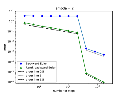
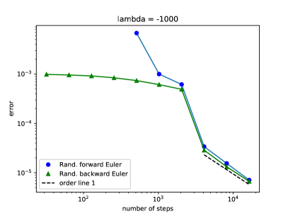
Figure 1. Left: $L^{2}$-convergence of the classical backward Euler method and scheme (4.1) to the IVP (5.1) with $\lambda=2$. Right: $L^{2}$-convergence of schemes (4.1) and (5.2) to (5.1) with $\lambda=-1000$.

In the numerical examples that lead to Figure 1, we considered the value $p=2^{-12}$ and step sizes $k=2^{-n}$ for $n\in\{5,\dots,14\}$. To evaluate the $L^{2}(\Omega;{\mathbf{R}})$-norm we considered $1000$ Monte Carlo iterations. In the plot on the left hand side we used the value $\lambda=2$ and compared the classical backward Euler method with scheme (4.1). As we expected from the discussion above, two different phases of the example become well visible. For $n\in\{5,\dots,11\}$ the classical backward Euler method does not offer an accurate numerical solution. The error of the randomized backward Euler method decreases with a rate of approximately $0.5$. When $n$ changes from $11$ to $12$ both schemes improve drastically since they are now able to fully resolve the oscillations of the solution. In the last part, for $n\in\{12,13,14\}$ the errors of both schemes decrease with a larger rate. Also here, the randomized scheme appears to have a higher rate of convergence, $1.5$, than the classical scheme which converges with rate $1$. Note that the rate of $1.5$ is in line with those of randomized quadrature rules, see [30].

In the plot on the right-hand side in Figure 1, we considered the case $\lambda=-1000$ and compared the randomized backward Euler method (4.1) with the randomized forward Euler method (5.2). Here, we only plotted errors smaller than $1$, since the explicit scheme produces strongly oscillating numerical solutions with a very large amplitude for step sizes which are not small enough. The first occurring error of the scheme (5.2) in the plot appears for $2^{9}=512$ temporal steps. This was expected since the explicit scheme only leads to a non-exploding solution for step sizes $k$ with $|1+k\lambda|<1$.

To sum up, the numerical experiments in this section indicate that the randomized backward Euler method is especially advantageous compared to deterministic methods if the problem has very irregular coefficients. Compared to explicit randomized Runge–Kutta methods such as (5.2) we also obtain more reliable results for rather large step sizes when considering problems with a dissipative structure. Both points qualify the scheme (4.1) for the numerical treatment of monotone evolution equations with time-irregular coefficients. This will be studied in more details in the following sections.

6. A non-autonomous nonlinear evolution equation with time-irregular coefficients

In this section, we now turn our attention to the second class of initial value problems we consider in this paper. More precisely, we are interested in non-autonomous and possibly nonlinear evolution equations of the form

(6.1) $$\begin{split}\begin{cases}\dot{u}(t)+{\mathcal{A}}(t)u(t)=f(t),\quad\text{for almost all }t\in(0,T],\\ u(0)=u_{0}.\end{cases}\end{split}$$

In order to make this rather abstract setting more precise, we start by introducing the real, separable Hilbert spaces $(V,(\cdot,\cdot)_{V},\|\cdot\|_{V})$ and $(H,(\cdot,\cdot)_{H},\|\cdot\|_{H})$. Here, we assume that the space $V$ is densely embedded in the space $H$. Thus, we obtain the Gelfand triple

$$V\stackrel{{\scriptstyle d}}{{\hookrightarrow}}H\cong H^{\ast}\stackrel{{\scriptstyle d}}{{\hookrightarrow}}V^{\ast},$$

where $H^{*}$ and $V^{*}$ are the dual spaces of $H$ and $V$, respectively. These spaces are equipped with the induced dual norms.

We impose the following conditions on ${\mathcal{A}}$. Note that, as it is customary, we usually write ${\mathcal{A}}(t)v$ instead of ${\mathcal{A}}(t,v)$.

Assumption 6.1.

The mapping ${\mathcal{A}}\colon[0,T]\times V\to V^{\ast}$ fulfills the conditions:

1. For every $v_{1},v_{2}\in V$ the mapping $[0,T]\ni t\mapsto\langle{\mathcal{A}}(t)v_{1},v_{2}\rangle_{V^{*},V}$ is measurable.

2. There exists a constant $M\geq 0$ such that $\|{\mathcal{A}}(t)0\|_{V^{*}}\leq M$ for every $t\in[0,T]$.

3. There exists $L\in(0,\infty)$ such that for all $t\in[0,T]$ it holds true that

   $$\|{\mathcal{A}}(t)v_{1}-{\mathcal{A}}(t)v_{2}\|_{V^{\ast}}\leq L\|v_{1}-v_{2}\|_{V},\quad\text{ for all }v_{1},v_{2}\in V.$$

4. There exists $\mu\in(0,\infty)$ such that for all $t\in[0,T]$ it holds true that

   $$\langle{\mathcal{A}}(t)v_{1}-{\mathcal{A}}(t)v_{2},v_{1}-v_{2}\rangle_{V^{\ast},V}\geq\mu\|v_{1}-v_{2}\|^{2}_{V},\quad\text{ for all }v_{1},v_{2}\in V.$$

Remark 6.2.

Instead of Assumption 6.1 (iv) we can ask for the weaker condition

1. There exist $\mu\in(0,\infty)$ and $\kappa\in[0,\infty)$ such that for all $t\in[0,T]$ it holds true that

   $$\langle{\mathcal{A}}(t)v_{1}-{\mathcal{A}}(t)v_{2},v_{1}-v_{2}\rangle_{V^{\ast},V}\geq\mu\|v_{1}-v_{2}\|^{2}_{V}-\kappa\|v_{1}-v_{2}\|^{2}_{H},$$

   for all $v_{1},v_{2}\in V$.

Using this Gårding-type inequality, the following proofs can be done in an analogous manner with a further application of Gronwall’s inequality. This additional argument leads to a constant $C$ in Theorem 6.7 below that grows exponentially in time. For simplicity we will only treat the case $\kappa=0$ in the following.

Before we analyze the convergence of the numerical scheme (6.5) defined below, let us recall the existence of a unique solution to the abstract problem (6.1). We will consider the concept of weak solutions for abstract non-autonomous problems of the form (6.1), i.e., we call a function

$$u\in\mathcal{W}(0,T)=\big{\{}v\in L^{2}(0,T;V)\,:\,\dot{v}\in L^{2}(0,T;V^{*})\big{\}}$$

a weak solution to (6.1) if $u(0)=u_{0}$ is fulfilled and if the integral equality

(6.2) $$\int_{0}^{T}\langle\dot{u}(t)+{\mathcal{A}}(t)u(t),v(t)\rangle_{V^{*},V}\,\mathrm{d}t=\int_{0}^{T}\langle f(t),v(t)\rangle_{V^{*},V}\,\mathrm{d}t$$

is satisfied for every $v\in L^{2}(0,T;V)$. Note that evaluating the abstract function $u$ at the initial time is well defined since the space $\mathcal{W}(0,T)$ is embedded in the space $C([0,T];H)$. An introduction to this concept of solutions can be found in, for example, [14], [16] or [37].

Proposition 6.3.

Let Assumption 6.1 be satisfied. Then for every given $f\in L^{2}(0,T;H)$ and initial value $u_{0}\in H$ there exists a unique weak solution $u\in\mathcal{W}(0,T)$ to the problem (6.1).

Most proofs for this kind of statement that can be found in the literature are either for linear problems, see for example [42, Cor. 23.26] or [14, Satz 8.3.6], or for nonlinear problems in a Browder–Minty setting, compare for example [43, Thm 30.A], [14, Satz 8.4.2] or [37, Theorem 8.9]. Our assertion is intermediate since we consider nonlinear operators that are still Lipschitz continuous. Therefore, the aforementioned references for nonlinear problems can be used but we note that also small modifications of the proofs for linear problems would be sufficient.

Remark 6.4.

Note that for mere existence results, it is sufficient to assume $f\in L^{2}(0,T;V^{*})+L^{1}(0,T;H)$. The last proposition and some of the following statements would also hold under this more general condition. To obtain a rate of convergence for the numerical scheme, the additional assumption $f\in L^{2}(0,T;H)$ will be essential.

In the following, we will consider a full discretization of the problem (6.1), i.e., we will discretize the equation both in time and space. For this purpose let $N\in{\mathbf{N}}$ denote the number of temporal steps and set $k=\frac{T}{N}$ as the temporal step size. For this particular $N$ and $k$ we obtain an equidistant partition of the interval $[0,T]$ given by $t_{n}:=kn$, $n\in\{0,\dots,N\}$. Further, we introduce the family of independent and $\mathcal{U}(0,1)$-distributed random variables $\tau=(\tau_{n})_{n\in{\mathbf{N}}}$ on a complete probability space $(\Omega,{\mathcal{F}},{\mathbf{P}})$ and write $\xi_{n}=t_{n}+k\tau_{n}$ for $n\in{\mathbf{N}}$. Let $({\mathcal{F}}_{n})_{n\in\{0,\dots,N\}}$ be the complete filtration which is induced by $(\xi_{n})_{n\in\{0,\dots,N\}}$, compare with (4.3).

For the space discretization we consider an abstract Galerkin method. To this end let $(V_{h})_{h\in(0,1)}$ be a sequence of finite-dimensional subspaces of $V$ each endowed with the inner product $(\cdot,\cdot)_{H}$ and the norm $\|\cdot\|_{H}$ of $H$. Further, for each $h\in(0,1)$ we denote by $P_{h}\colon H\to V_{h}$ the orthogonal projection onto the Galerkin space $V_{h}$ with respect to $(\cdot,\cdot)_{H}$. More precisely, for each $v\in H$ we define $P_{h}v$ as the uniquely determined element in $V_{h}$ that satisfies

(6.3) $$(P_{h}v,w_{h})_{H}=(v,w_{h})_{H},\quad\text{ for all }w_{h}\in V_{h}.$$

In order to formulate the equation (6.1) in a suitable discrete setting, we also introduce a discrete version ${\mathcal{A}}_{h}\colon[0,T]\times V_{h}\to V_{h}$ of the operator ${\mathcal{A}}$. This is accomplished in the same way as above by defining ${\mathcal{A}}_{h}(t)v_{h}$ for given $t\in[0,T]$ and $v_{h}\in V_{h}$ as the unique element in $V_{h}$ that fulfills

(6.4) $$\big{(}{\mathcal{A}}_{h}(t)v_{h},w_{h}\big{)}_{H}=\langle{\mathcal{A}}(t)v_{h},w_{h}\rangle_{V^{*},V}$$

for every $w_{h}\in V_{h}$. The existence of a unique ${\mathcal{A}}_{h}(t)v_{h}\in V_{h}$ follows directly from the Riesz representation theorem.

Our aim is to examine the numerical scheme

(6.5) $$\begin{split}\begin{cases}U^{n}_{h}+k{\mathcal{A}}_{h}(\xi_{n})U^{n}_{h}=kP_{h}f(\xi_{n})+U^{n-1}_{h},\quad\text{ for }n\in\{1,\ldots,N\},\\ U^{0}_{h}=P_{h}u_{0}.\end{cases}\end{split}$$

Note that, as in the finite-dimensional case in Section 4, the numerical approximation $(U^{n}_{h})_{n\in\{0,\dots,N\}}$ consists of a family of random variables taking values in $V_{h}$. Before we analyze the convergence of the scheme (6.5) the following lemma shows that $(U^{n}_{h})_{n\in\{0,\ldots,N\}}$ is indeed well-defined for every value of the step size $k$.

Lemma 6.5.

Let Assumption 6.1 be satisfied. Then for every inhomogeneity $f\in L^{2}(0,T;H)$, every initial value $u_{0}\in H$, and every step size $k=\frac{T}{N}$, $N\in{\mathbf{N}}$, there exists a unique solution $(U^{n}_{h})_{n\in\{0,\dots,N\}}$ to the implicit scheme (6.5) such that for every $n\in\{1,\ldots,N\}$ the element $U^{n}_{h}$ is ${\mathcal{F}}_{n}$-measurable and $U^{n}_{h}(\omega)\in V_{h}$ for almost every $\omega\in\Omega$.

Proof.

Let $h\in(0,1)$ be fixed. To prove the existence of a suitable solution to (6.5), we introduce an equivalent problem in ${\mathbf{R}}^{d}$ with $d=\dim(V_{h})$ such that we can apply arguments from Section 4 to prove the existence of a unique solution $(U^{n}_{h})_{n\in\{0,\dots,N\}}$. To this end, we consider a basis $\{\psi_{1},\dots,\psi_{d}\}$ of the finite-dimensional space $V_{h}$ and test (6.5) with a basis element $\psi_{j}$, $j\in\{1,\dots,d\}$. Then (6.5) can equivalently be rewritten as the following system of scalar equations

(6.6) $$\begin{split}\begin{cases}(U^{n}_{h}+k{\mathcal{A}}_{h}(\xi_{n})U^{n}_{h},\psi_{j})_{H}=(kP_{h}f(\xi_{n})+U^{n-1}_{h},\psi_{j})_{H},\quad\text{ for }n\in\{1,\ldots,N\},\\ (U_{h}^{0},\psi_{j})_{H}=(u_{0},\psi_{j})_{H},\end{cases}\end{split}$$

for all $j\in\{1,\ldots,d\}$. Since the inhomogeneity $P_{h}f\in L^{2}(0,T;V_{h})$ takes values in $V_{h}$ it can be represented by

$$P_{h}f=\sum_{i=1}^{d}f_{h,i}\psi_{i},$$

where $f_{h,i}\in L^{2}(0,T;{\mathbf{R}})$ for each $i\in\{1,\ldots,d\}$. In order to prove the existence of the $V_{h}$-valued random variable $U^{n}_{h}$, we will show that there exist measurable functions $\alpha^{n}_{h,i}\colon\Omega\to{\mathbf{R}}$, $i\in\{1,\ldots,d\}$, $n\in\{0,\ldots,N\}$, such that

$$U^{n}_{h}=\sum_{i=1}^{d}\alpha_{h,i}^{n}\psi_{i}$$

satisfies (6.5). For $n=0$ this follows at once.

For the case $n>0$ let us denote the vector of all coordinates $(\alpha^{n}_{h,i})_{i\in\{1,\ldots,d\}}$ and $(f_{h,i})_{i\in\{1,\ldots,d\}}$ by

$$\mathbf{u_{h}^{n}}(\omega):=\big{(}\alpha_{h,i}^{n}(\omega)\big{)}_{i\in\{1,\dots,d\}}\quad\text{and}\quad\mathbf{f_{h}}(t):=\big{(}f_{h,i}(t)\big{)}_{i\in\{1,\dots,d\}}$$

for almost every $\omega\in\Omega$ and $t\in[0,T]$. Furthermore, we denote the mass matrix in ${\mathbf{R}}^{d,d}$ by

$$\mathbf{M_{h}}=\big{(}(\psi_{i},\psi_{j})_{H}\big{)}_{i,j\in\{1,\dots,d\}}.$$

It is easily seen that $\mathbf{M_{h}}\in{\mathbf{R}}^{d,d}$ is symmetric and positive definite. In order to obtain a corresponding representation for ${\mathcal{A}}_{h}(t)\colon V_{h}\to V_{h}$, $t\in[0,T]$, we introduce $\mathbf{A_{h}}\colon[0,T]\times{\mathbf{R}}^{d}\to{\mathbf{R}}^{d}$ such that for $t\in[0,T]$ and $\mathbf{x}\in{\mathbf{R}}^{d}$ the vector $\mathbf{A_{h}}(t,\mathbf{x})\in{\mathbf{R}}^{d}$ is determined by

$$\sum_{i=1}^{d}\big{[}\mathbf{A_{h}}(t,\mathbf{x})\big{]}_{i}\psi_{i}={\mathcal{A}}_{h}(t)v_{\mathbf{x}}\in V_{h},$$

where $v_{\mathbf{x}}=\sum_{i=1}^{d}\mathbf{x}_{i}\psi_{i}$. Then (6.6) can equivalently be written as

$$\mathbf{M_{h}}\mathbf{u^{n}_{h}}+k\mathbf{M_{h}}\mathbf{A_{h}}(\xi_{n},\mathbf{u^{n}_{h}})=k\mathbf{M_{h}}\mathbf{f_{h}}(\xi_{n})+\mathbf{M_{h}}\mathbf{u^{n-1}_{h}},$$

or simply

$$\mathbf{u^{n}_{h}}=\mathbf{u^{n-1}_{h}}+k\big{(}\mathbf{f_{h}}(\xi_{n})-\mathbf{A_{h}}(\xi_{n},\mathbf{u^{n}_{h}})\big{)}.$$

In order to transfer the monotonicity and Lipschitz continuity of ${\mathcal{A}}_{h}$ to its counterpart, we introduce the following inner product and norm in ${\mathbf{R}}^{d}$:

$$(\mathbf{x},\mathbf{y})_{\mathbf{M_{h}}}=\mathbf{x}^{T}\mathbf{M_{h}}\mathbf{y}\quad\text{ and }\quad\|\mathbf{x}\|_{\mathbf{M_{h}}}=\sqrt{(\mathbf{x},\mathbf{x})_{\mathbf{M_{h}}}}$$

for $\mathbf{x},\mathbf{y}\in{\mathbf{R}}^{d}$. This particular choice of inner product coincides with the inner product of $H$ of the elements $u_{\mathbf{x}},v_{\mathbf{x}}\in H$ given by

$$u_{\mathbf{x}}=\sum_{i=1}^{d}\mathbf{x}_{i}\psi_{i}\quad\text{ and }\quad v_{\mathbf{y}}=\sum_{i=1}^{d}\mathbf{y}_{i}\psi_{i}$$

for $\mathbf{x},\mathbf{y}\in{\mathbf{R}}^{d}$, i.e., the following equalities hold:

$$(\mathbf{x},\mathbf{y})_{\mathbf{M_{h}}}=(u_{\mathbf{x}},v_{\mathbf{y}})_{H}\quad\text{and}\quad\|\mathbf{x}\|_{\mathbf{M_{h}}}=\|u_{\mathbf{x}}\|_{H}.$$

To prove the existence of an element $\mathbf{u^{n}_{h}}(\omega)$ for almost every $\omega\in\Omega$ we use Lemma 4.1. To this end, we introduce the function

$$\mathbf{g}\colon\Omega\times{\mathbf{R}}^{d}\to{\mathbf{R}}^{d},\quad\mathbf{g}(\omega,\mathbf{x})=\mathbf{x}-\mathbf{u^{n-1}_{h}}(\omega)-k\big{(}\mathbf{f_{h}}(\xi_{n}(\omega))-\mathbf{A_{h}}(\xi_{n}(\omega),\mathbf{x})\big{)}.$$

Define $q=q(\omega):=\|U^{n-1}_{h}(\omega)\|_{H}+k\|f(\xi_{n}(\omega))\|_{H}$. Observe that for almost every $\omega\in\Omega$ we have $q(\omega)\in[0,\infty)$. In the following we consider an arbitrary but fixed $\omega\in\Omega$ with this property. Next, we introduce

$$R=R(\omega)=\frac{q}{2}+\sqrt{\frac{q^{2}}{4}+k\frac{M^{2}}{4\mu}}\in(0,\infty).$$

For all $\mathbf{x}\in{\mathbf{R}}^{d}$ with $\|\mathbf{x}\|_{\mathbf{M_{h}}}=R$ we then obtain

$$(\mathbf{g}(\omega,\mathbf{x}),\mathbf{x})_{\mathbf{M_{h}}}$$

$$\quad=(\mathbf{x}-\mathbf{u^{n-1}_{h}}(\omega)-k\big{(}\mathbf{f_{h}}(\xi_{n}(\omega))-\mathbf{A_{h}}(\xi_{n}(\omega),\mathbf{x})\big{)},\mathbf{x})_{\mathbf{M_{h}}}$$

$$\quad=\|\mathbf{x}\|^{2}_{\mathbf{M_{h}}}-(\mathbf{u^{n-1}_{h}}(\omega),\mathbf{x})_{\mathbf{M_{h}}}-k(\mathbf{f_{h}}(\xi_{n}(\omega)),\mathbf{x})_{\mathbf{M_{h}}}+k(\mathbf{A_{h}}(\xi_{n}(\omega),\mathbf{x}),\mathbf{x})_{\mathbf{M_{h}}}$$

(6.7) $$\quad\geq R^{2}-R\|U^{n-1}_{h}(\omega)\|_{H}-kR\|f(\xi_{n}(\omega))\|_{H}+k\langle{\mathcal{A}}(\xi_{n}(\omega))v_{\mathbf{x}},v_{\mathbf{x}}\rangle_{V^{*},V}$$

where $v_{\mathbf{x}}=\sum_{i=1}^{d}\mathbf{x}_{i}\psi_{i}$. Using Assumption 6.1 (ii) and (iv), the last summand of (6.7) can be estimated by

(6.8) $$\begin{split}&\langle{\mathcal{A}}(\xi_{n}(\omega))v_{\mathbf{x}},v_{\mathbf{x}}\rangle_{V^{*},V}\\ &\quad=\langle{\mathcal{A}}(\xi_{n}(\omega))v_{\mathbf{x}}-{\mathcal{A}}(\xi_{n}(\omega))0,v_{\mathbf{x}}-0\rangle_{V^{*},V}+\langle{\mathcal{A}}(\xi_{n}(\omega))0,v_{\mathbf{x}}\rangle_{V^{*},V}\\ &\quad\geq\mu\|v_{\mathbf{x}}\|_{V}^{2}-\|{\mathcal{A}}(\xi_{n}(\omega))0\|_{V^{*}}\|v_{\mathbf{x}}\|_{V}\\ &\quad\geq\mu\|v_{\mathbf{x}}\|_{V}^{2}-M\|v_{\mathbf{x}}\|_{V}\\ &\quad\geq\mu\|v_{\mathbf{x}}\|_{V}^{2}-\frac{M^{2}}{4\mu}-\mu\|v_{\mathbf{x}}\|_{V}^{2}=-\frac{M^{2}}{4\mu}.\end{split}$$

Therefore, after inserting $R$ we obtain

$$(\mathbf{g}(\omega,\mathbf{x}),\mathbf{x})_{\mathbf{M_{h}}}\geq R^{2}-R\big{(}\|U^{n-1}_{h}(\omega)\|_{H}+k\|f(\xi_{n}(\omega))\|_{H}\big{)}-k\frac{M^{2}}{4\mu}=0.$$

Since $\mathbf{A_{h}}(\xi_{n}(\omega),\cdot)$ is continuous in the second argument due to Assumption 6.1 (iii), this allows us to apply Lemma 4.1 and Remark 4.2. Thus, for almost every $\omega\in\Omega$ we obtain the existence of an element $\mathbf{x}=\mathbf{x}(\omega)\in{\mathbf{R}}^{d}$ such that $\mathbf{g}(\omega,\mathbf{x})=0$ holds. To prove that this root is unique, assume that there exist $\mathbf{x},\mathbf{y}\in{\mathbf{R}}^{d}$ such that

$$\mathbf{g}(\omega,\mathbf{x})=0\quad\text{ and }\quad\mathbf{g}(\omega,\mathbf{y})=0$$

is fulfilled. Then, inserting the definition of the function $\mathbf{g}$ leads to

$$\|\mathbf{x}-\mathbf{y}\|_{\mathbf{M_{h}}}^{2} =-k(\mathbf{A_{h}}(\xi_{n}(\omega),\mathbf{x})-\mathbf{A_{h}}(\xi_{n}(\omega),\mathbf{y}),\mathbf{x}-\mathbf{y})_{\mathbf{M_{h}}}$$

$$=-k({\mathcal{A}}_{h}(\xi_{n}(\omega))v_{\mathbf{x}}-{\mathcal{A}}_{h}(\xi_{n}(\omega))v_{\mathbf{y}},v_{\mathbf{x}}-v_{\mathbf{y}})_{H}\leq 0.$$

This implies $\mathbf{x}=\mathbf{y}$. An application of Lemma 4.3 then yields that the mapping

$$\mathbf{u_{h}^{n}}\colon\Omega\to{\mathbf{R}}^{d},\quad\omega\mapsto\mathbf{u_{h}^{n}}(\omega)=\big{(}\alpha_{h,i}^{n}(\omega)\big{)}_{i\in\{1,\dots,d\}}$$

is ${\mathcal{F}}_{n}$-measurable, where $\mathbf{u_{h}^{n}}(\omega)=\mathbf{x}(\omega)$ is the unique root of $\mathbf{g}(\omega,\cdot)$. To sum up,

$$U^{n}_{h}=\sum_{i=1}^{d}\alpha_{h,i}^{n}\psi_{i},\quad n\in\{0,\dots,N\},$$

is the well-defined solution to the scheme (6.5). Since $\{\psi_{1},\dots,\psi_{d}\}$ is a basis of $V_{h}$ this implies that $U^{n}_{h}(\omega)\in V_{h}$ for almost every $\omega\in\Omega$ and all $n\in\{0,\dots,N\}$. ∎

Lemma 6.6.

Let Assumption 6.1 be satisfied. Then for every $f\in L^{2}(0,T;H)$, every initial value $U_{h}^{0}\in V_{h}$, and every step size $k=\frac{T}{N}$, $N\in{\mathbf{N}}$, the unique solution $(U^{n}_{h})_{n\in\{0,\dots,N\}}$ to the implicit scheme (6.5) satisfies the a priori bound

$$\max_{n\in\{0,\ldots,N\}}{\mathbf{E}}\big{[}\|U_{h}^{n}\|_{H}^{2}\big{]}+\sum_{j=1}^{N}{\mathbf{E}}\big{[}\|U_{h}^{j}-U_{h}^{j-1}\|_{H}^{2}\big{]}+k\mu\sum_{j=1}^{N}{\mathbf{E}}\big{[}\|U_{h}^{j}\|_{V}^{2}\big{]}$$

$$\qquad\leq C\big{(}T+\|U_{h}^{0}\|_{H}^{2}+\|f\|_{L^{2}(0,T;H)}^{2}\big{)},$$

where the constant $C$ only depends on $M$, $\mu$, and the embedding $V\hookrightarrow H$.

Proof.

Due to the definition of scheme (6.5) we can write for every $j\in\{1,\ldots,N\}$

$$\frac{1}{k}\big{(}U_{h}^{j}-U_{h}^{j-1}\big{)}+{\mathcal{A}}_{h}(\xi_{j})U_{h}^{j}=f(\xi_{j}).$$

We test this equation with $U_{h}^{j}$ in the $H$ inner product and apply the polarization identity

$$\frac{1}{2}\big{(}\|U_{h}^{j}\|_{H}^{2}-\|U_{h}^{j-1}\|^{2}_{H}+\|U_{h}^{j}-U_{h}^{j-1}\|_{H}^{2}\big{)}=(U_{h}^{j}-U_{h}^{j-1},U_{h}^{j})_{H}.$$

In addition, recall from (6.4) and (6.8) that

$$\big{(}{\mathcal{A}}_{h}(\xi_{j})U^{j}_{h},U^{j}_{h}\big{)}_{H}=\big{\langle}{\mathcal{A}}(\xi_{j})U^{j}_{h},U^{j}_{h}\big{\rangle}_{V^{\ast},V}\geq\mu\big{\|}U_{h}^{j}\big{\|}_{V}^{2}-\big{\|}{\mathcal{A}}(\xi_{j})0\big{\|}_{V^{\ast}}\big{\|}U_{h}^{j}\big{\|}_{V}.$$

From this and (6.5) as well as from Assumption 6.1 (ii) we obtain that

$$\frac{1}{2k}\big{(}\|U_{h}^{j}\|_{H}^{2}-\|U_{h}^{j-1}\|_{H}^{2}+\|U_{h}^{j}-U_{h}^{j-1}\|_{H}^{2}\big{)}+\mu\|U_{h}^{j}\|_{V}^{2}$$

$$\quad\leq\frac{1}{k}(U_{h}^{j}-U_{h}^{j-1},U_{h}^{j})_{H}+({\mathcal{A}}_{h}(\xi_{j})U_{h}^{j},U_{h}^{j})_{H}+\big{\|}{\mathcal{A}}(\xi_{j})0\big{\|}_{V^{\ast}}\big{\|}U_{h}^{j}\big{\|}_{V}$$

$$\quad=(f(\xi_{j}),U_{h}^{j})_{H}+M\big{\|}U_{h}^{j}\big{\|}_{V}$$

$$\quad\leq\|f(\xi_{j})\|_{H}\|U_{h}^{j}\|_{H}+M\|U_{h}^{j}\|_{V}$$

$$\quad\leq C\big{(}1+\|f(\xi_{j})\|_{H}^{2}\big{)}+\frac{\mu}{2}\|U_{h}^{j}\|_{V}^{2},$$

where the constant $C$ only depends on $M$, $\mu$, and the embedding $V\hookrightarrow H$. Next we sum up with respect to $j$ from $1$ to $n$ and obtain

$$\|U_{h}^{n}\|_{H}^{2}+\sum_{j=1}^{n}\|U_{h}^{j}-U_{h}^{j-1}\|_{H}^{2}+k\mu\sum_{j=1}^{n}\|U_{h}^{j}\|_{V}^{2}\leq\|U_{h}^{0}\|_{H}^{2}+k2C\sum_{j=1}^{n}\big{(}1+\|f(\xi_{j})\|_{H}^{2}\big{)}.$$

Taking the expectation, we further obtain for the term containing the inhomogeneity $f$ that

$${\mathbf{E}}\Big{[}k\sum_{j=1}^{n}\|f(\xi_{j})\|_{H}^{2}\Big{]}=\sum_{j=1}^{n}\int_{t_{j-1}}^{t_{j}}\|f(t)\|_{H}^{2}\,\mathrm{d}t\leq\big{\|}f\big{\|}_{L^{2}(0,T;H)}^{2}$$

holds. This completes the proof. ∎

After these preparatory results we can now state the abstract convergence result for the numerical method (6.5). For its formulation we define for each $v\in H$

(6.9) $$\mathrm{dist}_{H}(v,V_{h}) :=\inf_{v_{h}\in V_{h}}\|v-v_{h}\|_{H}.$$

Similarly, if $v\in V$ we set

(6.10) $$\mathrm{dist}_{V}(v,V_{h}) :=\inf_{v_{h}\in V_{h}}\|v-v_{h}\|_{V}.$$

With (6.9) we therefore measure how well a given element $v\in H$ can be approximated by elements from $V_{h}$. Since $V_{h}$ is finite-dimensional it is clear that $P_{h}v\in V_{h}$ has the best approximation properties with respect to the $H$-norm, that is

(6.11) $$\|P_{h}v-v\|_{H}=\mathrm{dist}_{H}(v,V_{h}),\quad\text{ for all }v\in H.$$

In the same way, if we define $Q_{h}\colon V\to V_{h}$ as the orthogonal projection onto $V_{h}$ with respect to the inner product $(\cdot,\cdot)_{V}$, then it holds true that

(6.12) $$\|Q_{h}v-v\|_{V}=\mathrm{dist}_{V}(v,V_{h}),\quad\text{ for all }v\in V.$$

Since we consider a general Galerkin method in this section we will not quantify the best approximation property of $(V_{h})_{h\in(0,1)}$ at this point.

We also mention that the error estimate in Theorem 6.7 requires the boundedness of $\|P_{h}\|_{{\mathcal{L}}(V)}$. However, one cannot expect in general that $\sup_{h\in(0,1]}\|P_{h}\|_{{\mathcal{L}}(V)}<\infty$. For a discussion of the stability of the orthogonal projector $P_{h}$ in case of the Galerkin finite element method we refer to [6, 7, 8, 11].

Theorem 6.7.

Let Assumption 6.1 be satisfied. Then for a given inhomogeneity $f\in L^{2}(0,T;H)$ and initial value $u_{0}\in V$ let $u$ be the unique weak solution to the abstract problem (6.1). In addition, we assume that there exists $\gamma\in(0,1)$ with

(6.13) $$u\in C^{\gamma}([0,T];V)$$

as well as

(6.14) $$\int_{0}^{T}\|{\mathcal{A}}(t)u(t)\|^{2}_{H}\,\mathrm{d}t<\infty.$$

Then there exists a constant $C$ only depending on $L$, $\mu$, and $T$ such that for every step size $k=\frac{T}{N}$, $N\in{\mathbf{N}}$, and $h\in(0,1)$ we have

$$\max_{n\in\{0,\dots,N\}}\|U^{n}_{h}-u(t_{n})\|_{L^{2}(\Omega;H)}+\Big{(}k\sum_{n=1}^{N}\|U^{n}_{h}-u(t_{n})\|_{L^{2}(\Omega;V)}^{2}\Big{)}^{\frac{1}{2}}$$

$$\quad\leq C\Big{(}k^{\frac{1}{2}}\big{(}\|f\|_{L^{2}(0,T;H)}+\|{\mathcal{A}}(\cdot)u(\cdot)\|_{L^{2}(0,T;H)}\big{)}+k^{\gamma}\|u\|_{C^{\gamma}([0,T];V)}$$

$$\qquad+\max_{n\in\{0,\dots,N\}}\mathrm{dist}_{H}(u(t_{n}),V_{h})+\big{(}1+\|P_{h}\|_{{\mathcal{L}}(V)}\big{)}\Big{(}k\sum_{n=1}^{N}\mathrm{dist}_{V}(u(t_{n}),V_{h})^{2}\Big{)}^{\frac{1}{2}}\Big{)},$$

where $(U^{n}_{h})_{n\in\{0,\ldots,N\}}\subset L^{2}(\Omega;V_{h})$ is given by the scheme (6.5).

Proof.

Throughout the proof we consider an arbitrary but fixed finite-dimensional subspace $V_{h}$, $h\in(0,1)$, of $V$. Moreover, we denote the error of the scheme (6.5) at the time $t_{n}$ by $E^{n}$, i.e., $E^{n}:=U^{n}_{h}-u(t_{n})$ for each $n\in\{0,\dots,N\}$. Note that for every $n\geq 1$ we have $E^{n}\in L^{2}(\Omega;V)$ since $U^{n}_{h}\in L^{2}(\Omega;V_{h})$ by Lemma 6.5 and Lemma 6.6. In addition, due to (6.13) we have $u(t)\in V$ for every $t\in[0,T]$.

In the first step, we split the error into two parts using the orthogonal projection $P_{h}\colon H\to V_{h}$ by

$$E^{n}=P_{h}E^{n}+(I-P_{h})E^{n}=:\Theta^{n}+\Xi^{n}.$$

Due to the orthogonality of $P_{h}$ with respect to the inner product in $H$ we have

$$\|E^{n}\|^{2}_{H}=\|\Theta^{n}\|^{2}_{H}+\|\Xi^{n}\|_{H}^{2}$$

for every $n\in\{0,\ldots,N\}$. By taking note of (6.11) we obtain

$$\|\Xi^{n}\|_{H}=\mathrm{dist}_{H}(u(t_{n}),V_{h})$$

since $\Xi^{n}=(I-P_{h})E^{n}=(P_{h}-I)u(t_{n})$. In addition, we have

$$\Big{(}k\sum_{n=1}^{N}\big{\|}E^{n}\big{\|}_{L^{2}(\Omega;V)}^{2}\Big{)}^{\frac{1}{2}}\leq\Big{(}k\sum_{n=1}^{N}\big{\|}\Theta^{n}\big{\|}_{L^{2}(\Omega;V)}^{2}\Big{)}^{\frac{1}{2}}+\Big{(}k\sum_{n=1}^{N}\big{\|}\Xi^{n}\big{\|}_{V}^{2}\Big{)}^{\frac{1}{2}}$$

since $\Xi^{n}=(P_{h}-I)u(t_{n})$ is deterministic. After adding and subtracting the orthogonal projector $Q_{h}\colon V\to V_{h}$ we further obtain the estimate

$$\big{\|}\Xi^{n}\big{\|}_{V} =\big{\|}(P_{h}-I)u(t_{n})\big{\|}_{V}\leq\big{\|}P_{h}(I-Q_{h})u(t_{n})\big{\|}_{V}+\big{\|}(Q_{h}-I)u(t_{n})\big{\|}_{V}$$

$$\leq\big{(}1+\|P_{h}\|_{{\mathcal{L}}(V)}\big{)}\|(Q_{h}-I)u(t_{n})\|=\big{(}1+\|P_{h}\|_{{\mathcal{L}}(V)}\big{)}\mathrm{dist}_{V}(u(t_{n}),V_{h}),$$

due to (6.12). This shows that

(6.15) $$k\sum_{n=1}^{N}\big{\|}\Xi^{n}\big{\|}_{V}^{2}\leq\big{(}1+\|P_{h}\|_{{\mathcal{L}}(V)}\big{)}^{2}k\sum_{n=1}^{N}\mathrm{dist}_{V}(u(t_{n}),V_{h})^{2}.$$

Thus it remains to estimate ${\mathbf{E}}[\|\Theta^{n}\|^{2}_{H}]$ and $k\sum_{n=1}^{N}{\mathbf{E}}[\|\Theta^{n}\|^{2}_{V}]$. To this end, we apply the polarization identity

(6.16) $$\frac{1}{2}\big{(}\|\Theta^{n}\|^{2}_{H}-\|\Theta^{n-1}\|^{2}_{H}+\|\Theta^{n}-\Theta^{n-1}\|^{2}_{H}\big{)}=(\Theta^{n}-\Theta^{n-1},\Theta^{n})_{H},$$

which holds for every $n\in\{1,\ldots,N\}$. From the orthogonality of $P_{h}$ with respect to the inner product in $H$ we further have

$$(\Theta^{n}-\Theta^{n-1},\Theta^{n})_{H}=(E^{n}-E^{n-1},\Theta^{n})_{H}$$

which motivates us to consider the term $E^{n}-E^{n-1}$ tested with $\Theta^{n}$ in what follows.

To estimate the difference of the errors $E^{n}-E^{n-1}=U^{n}_{h}-u(t_{n})-U^{n-1}_{h}+u(t_{n-1})$ we insert the definition of the scheme (6.5) and (6.3). This yields

$$\big{(}U^{n}_{h}-U^{n-1}_{h},\Theta^{n}\big{)}_{H} =k\big{(}P_{h}f(\xi_{n})-{\mathcal{A}}_{h}(\xi_{n})U^{n}_{h},\Theta^{n}\big{)}_{H}$$

$$=k\big{(}f(\xi_{n}),\Theta^{n}\big{)}_{H}-k\big{\langle}{\mathcal{A}}(\xi_{n})U^{n}_{h},\Theta^{n}\big{\rangle}_{V^{\ast},V}.$$

Moreover, since the random variable $\Theta^{n}$ takes values in $V_{h}\subset V$ we get from the canonical embedding $H\cong H^{\ast}\hookrightarrow V^{\ast}$ and (6.2) that

$$\big{(}u(t_{n})-u(t_{n-1}),\Theta^{n}\big{)}_{H} =\big{\langle}u(t_{n})-u(t_{n-1}),\Theta^{n}\big{\rangle}_{V^{\ast},V}$$

$$=\int_{t_{n-1}}^{t_{n}}\big{\langle}\dot{u}(s),\Theta^{n}\big{\rangle}_{V^{\ast},V}\,\mathrm{d}s$$

$$=\int_{t_{n-1}}^{t_{n}}\big{\langle}f(s)-{\mathcal{A}}(s)u(s),\Theta^{n}\big{\rangle}_{V^{\ast},V}\,\mathrm{d}s.$$

Therefore, altogether we obtain the following representation

(6.17) $$\begin{split}(E^{n}-E^{n-1},\Theta^{n})_{H}&=-k\big{\langle}{\mathcal{A}}(\xi_{n})U^{n}_{h}-{\mathcal{A}}(\xi_{n})u(t_{n}),\Theta^{n}\rangle_{V^{\ast},V}\\ &\qquad-k\big{\langle}{\mathcal{A}}(\xi_{n})u(t_{n})-{\mathcal{A}}(\xi_{n})u(\xi_{n}),\Theta^{n}\big{\rangle}_{V^{\ast},V}\\ &\qquad-\int_{t_{n-1}}^{t_{n}}\big{\langle}{\mathcal{A}}(\xi_{n})u(\xi_{n})-{\mathcal{A}}(s)u(s),\Theta^{n}\big{\rangle}_{V^{\ast},V}\,\mathrm{d}s\\ &\qquad+\int_{t_{n-1}}^{t_{n}}\big{(}f(\xi_{n})-f(s),\Theta^{n}\big{)}_{H}\,\mathrm{d}s\\ &=:\Gamma_{1}+\Gamma_{2}+\Gamma_{3}+\Gamma_{4}.\end{split}$$

We give estimates for the four terms $\Gamma_{i}$, $i\in\{1,\ldots,4\}$, in (6.17) separately. By recalling $\Theta^{n}=P_{h}E^{n}=U_{h}^{n}-P_{h}u(t_{n})$ the first term is estimated using Assumption 6.1 (iii) and (iv) as follows:

(6.18) $$\begin{split}\Gamma_{1}&=-k\big{\langle}{\mathcal{A}}(\xi_{n})U^{n}_{h}-{\mathcal{A}}(\xi_{n})P_{h}u(t_{n}),\Theta^{n}\big{\rangle}_{V^{\ast},V}\\ &\qquad-k\big{\langle}{\mathcal{A}}(\xi_{n})P_{h}u(t_{n})-{\mathcal{A}}(\xi_{n})u(t_{n}),\Theta^{n}\big{\rangle}_{V^{\ast},V}\\ &\leq-k\mu\big{\|}\Theta^{n}\big{\|}^{2}_{V}+kL\big{\|}(I-P_{h})u(t_{n})\big{\|}_{V}\big{\|}\Theta^{n}\big{\|}_{V}\\ &\leq-k\mu\big{\|}\Theta^{n}\big{\|}^{2}_{V}+k\frac{L^{2}}{\mu}\big{\|}\Xi^{n}\big{\|}_{V}^{2}+k\frac{\mu}{4}\big{\|}\Theta^{n}\big{\|}^{2}_{V}.\end{split}$$

Observe that we also applied the weighted Young inequality in the last step.

We similarly obtain an estimate for the second summand in (6.17) of the form

$$\Gamma_{2}\leq k\big{\|}{\mathcal{A}}(\xi_{n})u(t_{n})-{\mathcal{A}}(\xi_{n})u(\xi_{n})\big{\|}_{V^{\ast}}\big{\|}\Theta^{n}\big{\|}_{V}$$

$$\quad\leq k\frac{L^{2}}{\mu}\|u(t_{n})-u(\xi_{n})\|_{V}^{2}+k\frac{\mu}{4}\big{\|}\Theta^{n}\big{\|}_{V}^{2}.$$

Since $|t_{n}-\xi_{n}(\omega)|\leq k$ for every $\omega\in\Omega$ and $u\in C^{\gamma}([0,T];V)$ we therefore conclude

(6.19) $$\Gamma_{2}\leq k^{1+2\gamma}\frac{L^{2}}{\mu}\|u\|_{C^{\gamma}([0,T];V)}^{2}+k\frac{\mu}{4}\big{\|}\Theta^{n}\big{\|}_{V}^{2}.$$

Concerning the term $\Gamma_{3}$ in (6.17), let us recall that both $\Theta^{n}$ and $\xi_{n}$ are square-integrable random variables which are ${\mathcal{F}}_{n}$-measurable. Moreover, $\Theta^{n}$ takes values in $V_{h}\subset V$, while $\omega\mapsto{\mathcal{A}}(\xi_{n}(\omega))u(\xi_{n}(\omega))$ takes almost surely values in $H$ due to (6.14). Therefore, after taking expectation we obtain

(6.20) $$\begin{split}{\mathbf{E}}\big{[}\Gamma_{3}\big{]}&={\mathbf{E}}\Big{[}\int_{t_{n-1}}^{t_{n}}\big{\langle}{\mathcal{A}}(\xi_{n})u(\xi_{n})-{\mathcal{A}}(s)u(s),\Theta^{n}\big{\rangle}_{V^{\ast},V}\,\mathrm{d}s\Big{]}\\ &={\mathbf{E}}\Big{[}\int_{t_{n-1}}^{t_{n}}\big{(}{\mathcal{A}}(\xi_{n})u(\xi_{n})-{\mathcal{A}}(s)u(s),\Theta^{n}\big{)}_{H}\,\mathrm{d}s\Big{]}\\ &={\mathbf{E}}\Big{[}\int_{t_{n-1}}^{t_{n}}\big{(}{\mathcal{A}}(\xi_{n})u(\xi_{n})-{\mathcal{A}}(s)u(s),\Theta^{n}-\Theta^{n-1}\big{)}_{H}\,\mathrm{d}s\Big{]}\\ &\quad+{\mathbf{E}}\Big{[}\int_{t_{n-1}}^{t_{n}}\big{(}{\mathcal{A}}(\xi_{n})u(\xi_{n})-{\mathcal{A}}(s)u(s),\Theta^{n-1}\big{)}_{H}\,\mathrm{d}s\Big{]}.\end{split}$$

Standard arguments then directly yield a bound for the first summand of the form

$${\mathbf{E}}\Big{[}\int_{t_{n-1}}^{t_{n}}\big{(}{\mathcal{A}}(\xi_{n})u(\xi_{n})-{\mathcal{A}}(s)u(s),\Theta^{n}-\Theta^{n-1}\big{)}_{H}\,\mathrm{d}s\Big{]}$$

$$\quad\leq\Big{(}{\mathbf{E}}\Big{[}\int_{t_{n-1}}^{t_{n}}\|{\mathcal{A}}(\xi_{n})u(\xi_{n})-{\mathcal{A}}(s)u(s)\|^{2}_{H}\,\mathrm{d}s\Big{]}\Big{)}^{\frac{1}{2}}\big{(}k{\mathbf{E}}\big{[}\|\Theta^{n}-\Theta^{n-1}\|^{2}_{H}\big{]}\big{)}^{\frac{1}{2}}$$

$$\quad\leq k{\mathbf{E}}\Big{[}\int_{t_{n-1}}^{t_{n}}\|{\mathcal{A}}(\xi_{n})u(\xi_{n})-{\mathcal{A}}(s)u(s)\|^{2}_{H}\,\mathrm{d}s\Big{]}+\frac{1}{4}{\mathbf{E}}\big{[}\|\Theta^{n}-\Theta^{n-1}\|^{2}_{H}\big{]}$$

$$\quad\leq 4k\int_{t_{n-1}}^{t_{n}}\|{\mathcal{A}}(s)u(s)\|^{2}_{H}\,\mathrm{d}s+\frac{1}{4}{\mathbf{E}}\big{[}\|\Theta^{n}-\Theta^{n-1}\|^{2}_{H}\big{]},$$

where the last step follows from

$${\mathbf{E}}\big{[}k\|{\mathcal{A}}(\xi_{n})u(\xi_{n})\|^{2}_{H}\big{]}=\int_{t_{n-1}}^{t_{n}}\|{\mathcal{A}}(s)u(s)\|^{2}_{H}\,\mathrm{d}s.$$

To estimate the second summand in (6.20), we make use of the tower property for conditional expectations and the fact that $\Theta^{n-1}$ is ${\mathcal{F}}_{n-1}$-measurable. This yields

$${\mathbf{E}}\Big{[}\int_{t_{n-1}}^{t_{n}}\big{(}{\mathcal{A}}(\xi_{n})u(\xi_{n})-{\mathcal{A}}(s)u(s),\Theta^{n-1}\big{)}_{H}\,\mathrm{d}s\Big{]}$$

$$\quad={\mathbf{E}}\Big{[}\int_{t_{n-1}}^{t_{n}}{\mathbf{E}}\big{[}\big{(}{\mathcal{A}}(\xi_{n})u(\xi_{n})-{\mathcal{A}}(s)u(s),\Theta^{n-1}\big{)}_{H}\big{|}{\mathcal{F}}_{n-1}\big{]}\,\mathrm{d}s\Big{]}$$

$$\quad={\mathbf{E}}\Big{[}k{\mathbf{E}}\big{[}\big{(}{\mathcal{A}}(\xi_{n})u(\xi_{n}),\Theta^{n-1}\big{)}_{H}\big{|}{\mathcal{F}}_{n-1}\big{]}-\int_{t_{n-1}}^{t_{n}}\big{(}{\mathcal{A}}(s)u(s),\Theta^{n-1}\big{)}_{H}\,\mathrm{d}s\Big{]}=0,$$

where the last step follows from

$$k{\mathbf{E}}\big{[}\big{(}{\mathcal{A}}(\xi_{n})u(\xi_{n}),\Theta^{n-1}\big{)}_{H}\big{|}{\mathcal{F}}_{n-1}\big{]} =\big{(}k{\mathbf{E}}\big{[}{\mathcal{A}}(\xi_{n})u(\xi_{n})\big{|}{\mathcal{F}}_{n-1}\big{]},\Theta^{n-1}\big{)}_{H}$$

$$=\big{(}k{\mathbf{E}}\big{[}{\mathcal{A}}(\xi_{n})u(\xi_{n})\big{]},\Theta^{n-1}\big{)}_{H}$$

$$=\int_{t_{n-1}}^{t_{n}}\big{(}{\mathcal{A}}(s)u(s),\Theta^{n-1}\big{)}_{H}\,\mathrm{d}s$$

due to the independence of $\xi_{n}$ from ${\mathcal{F}}_{n-1}$. Altogether this shows

(6.21) $${\mathbf{E}}\big{[}\Gamma_{3}\big{]}\leq 4k\int_{t_{n-1}}^{t_{n}}\|{\mathcal{A}}(s)u(s)\|^{2}_{H}\,\mathrm{d}s+\frac{1}{4}{\mathbf{E}}\big{[}\|\Theta^{n}-\Theta^{n-1}\|^{2}_{H}\big{]}.$$

The same steps with $f(\cdot)$ in place of ${\mathcal{A}}(\cdot)u(\cdot)$ also yield an estimate for $\Gamma_{4}$. Therefore,

(6.22) $${\mathbf{E}}\big{[}\Gamma_{4}\big{]}\leq 4k\int_{t_{n-1}}^{t_{n}}\|f(s)\|^{2}_{H}\,\mathrm{d}s+\frac{1}{4}{\mathbf{E}}\big{[}\|\Theta^{n}-\Theta^{n-1}\|^{2}_{H}\big{]}.$$

In summary, after taking expectation and inserting (6.18), (6.19), (6.21), and (6.22) into (6.16) we obtain

$$\frac{1}{2}{\mathbf{E}}\big{[}\|\Theta^{n}\|^{2}_{H}-\|\Theta^{n-1}\|^{2}_{H}+\|\Theta^{n}-\Theta^{n-1}\|^{2}_{H}\big{]}$$

$$\quad={\mathbf{E}}\big{[}\Gamma_{1}+\Gamma_{2}+\Gamma_{3}+\Gamma_{4}\big{]}$$

$$\quad\leq-\frac{1}{2}k\mu{\mathbf{E}}\big{[}\big{\|}\Theta^{n}\big{\|}^{2}_{V}\big{]}+k\frac{L^{2}}{\mu}\big{\|}\Xi^{n}\big{\|}_{V}^{2}+k^{1+2\gamma}\frac{L^{2}}{\mu}\|u\|_{C^{\gamma}([0,T];V)}^{2}$$

$$\qquad+4k\int_{t_{n-1}}^{t_{n}}\|{\mathcal{A}}(s)u(s)\|^{2}_{H}\,\mathrm{d}s+4k\int_{t_{n-1}}^{t_{n}}\|f(s)\|^{2}_{H}\,\mathrm{d}s$$

$$\qquad+\frac{1}{2}{\mathbf{E}}\big{[}\|\Theta^{n}-\Theta^{n-1}\|^{2}_{H}\big{]}.$$

After canceling the last term from both sides of the inequality, we sum over $n\in\{1,\ldots,j\}$ for some arbitrary $j\in\{1,\ldots,N\}$. Moreover, since $U_{h}^{0}=P_{h}u_{0}$ we also have $\Theta^{0}=0$. Hence we obtain

$${\mathbf{E}}\big{[}\|\Theta^{j}\|^{2}_{H}\big{]}+\frac{1}{2}k\mu\sum_{n=1}^{j}{\mathbf{E}}\big{[}\|\Theta^{n}\|^{2}_{V}\big{]}$$

$$\quad\leq k\frac{L^{2}}{\mu}\sum_{n=1}^{j}\big{\|}\Xi^{j}\big{\|}_{V}^{2}+k^{2\gamma}T\frac{L^{2}}{\mu}\|u\|_{C^{\gamma}([0,T];V)}^{2}$$

$$\qquad+4k\big{(}\|{\mathcal{A}}(\cdot)u(\cdot)\|^{2}_{L^{2}(0,T;H)}+\|f\|_{L^{2}(0,T;H)}^{2}\big{)}.$$

The proof is completed by taking the maximum over $j\in\{1,\ldots,N\}$ and an application of (6.15). ∎

Remark 6.8.

Let us briefly discuss the additional regularity conditions (6.13) and (6.14) in Theorem 6.7. First note that since $f\in L^{2}(0,T;H)$ the condition (6.14) is essentially equivalent to

$$\dot{u}\in L^{2}(0,T;H).$$

A sufficient condition for (6.13) is then to additionally require

$$\dot{u}=f-{\mathcal{A}}(\cdot)u(\cdot)\in L^{q}(0,T;V)$$

with $q=\frac{1}{1-\gamma}$. In Section 7 we will discuss more explicit classes of linear and semilinear evolution equations, whose solutions enjoy the required regularity.

7. Regularity of non-autonomous evolution equations

To prove a rate of convergence in Section 6, we had to to impose additional assumptions on the regularity of the exact solution $u$. In the following, we will discuss cases where this particular regularity can be expected.

We begin by considering a class of linear problems that fulfills the regularity conditions imposed in Theorem 6.7. As in Section 6, we consider the real, separable Hilbert spaces $(V,(\cdot,\cdot)_{V},\|\cdot\|_{V})$ and $(H,(\cdot,\cdot)_{H},\|\cdot\|_{H})$ that form the Gelfand triple

$$V\stackrel{{\scriptstyle c,d}}{{\hookrightarrow}}H\cong H^{*}\stackrel{{\scriptstyle c,d}}{{\hookrightarrow}}V^{*}.$$

Further, we state the following assumption to obtain a suitable evolution operator.

Assumption 7.1.

For all $t\in[0,T]$ let $a_{0}(t;\cdot,\cdot)\colon V\times V\to{\mathbf{R}}$ be a bilinear form that fulfills the following conditions:

1. For every $v_{1},v_{2}\in V$ the mapping $a_{0}(\cdot;v_{1},v_{2})\colon[0,T]\to{\mathbf{R}}$ is measurable.

2. There exists $\beta\in(0,\infty)$ such that for all $t\in[0,T]$ it holds true that

   $$|a_{0}(t;v_{1},v_{2})|\leq\beta\|v_{1}\|_{V}\|v_{2}\|_{V},\quad\text{ for all }v_{1},v_{2}\in V.$$

3. There exists $\mu\in(0,\infty)$ such that for all $t\in[0,T]$ it holds true that

   $$a_{0}(t;v,v)\geq\mu\|v\|^{2}_{V},\quad\text{ for all }v\in V.$$

For every $t\in[0,T]$ let ${\mathcal{A}}_{0}(t)\colon V\to V^{*}$ and $A_{0}(t)\colon{\mathrm{dom}}(A_{0}(t))\subset H\to H$ denote the associated operators to the bilinear form $a_{0}(t;\cdot,\cdot)$ from Assumption 7.1. More precisely, the linear operator ${\mathcal{A}}_{0}(t)$ is uniquely determined by

$$\big{\langle}{\mathcal{A}}_{0}(t)v_{1},v_{2}\big{\rangle}_{V^{\ast},V} =a_{0}(t;v_{1},v_{2}),\quad\text{ for all }v_{1},v_{2}\in V.$$

Moreover, we set ${\mathrm{dom}}(A_{0}(t)):=\{v\in V\,:\,{\mathcal{A}}_{0}(t)v\in H\}$ and define $A_{0}(t)$ as the restriction of ${\mathcal{A}}_{0}(t)$ to the domain ${\mathrm{dom}}(A_{0}(t))$. Note that ${\mathrm{dom}}(A_{0}(t))$ becomes a Banach space if endowed with the graph norm. For given $u_{0}\in V$ and $f\in L^{2}(0,T;H)$ we consider the following linear and non-autonomous problem

(7.1) $$\begin{split}\begin{cases}\dot{u}(t)+{\mathcal{A}}_{0}(t)u(t)=f(t),&\quad t\in(0,T],\\ u(0)=u_{0}.&\end{cases}\end{split}$$

For the formulation of the regularity result we first recall that the initial value problem (7.1) is said to have maximal $L^{p}$-regularity in $H$ for some $p\in[2,\infty)$ if for all $f\in L^{p}(0,T;H)$ we have a unique solution $u\in\mathcal{W}(0,T)$ with $\dot{u}\in L^{p}(0,T;H)$ and ${\mathcal{A}}_{0}(\cdot)u(\cdot)\in L^{p}(0,T;H)$.

Theorem 7.2.

For every $t\in[0,T]$ let $a_{0}(t;\cdot,\cdot)\colon V\times V\to{\mathbf{R}}$ fulfill Assumption 7.1. Suppose there exists $M\geq 0$ such that $\|A_{0}(0)A_{0}^{-1}(t)\|_{{\mathcal{L}}(H)}\leq M$ holds true for all $t\in[0,T]$, that the embedding ${\mathrm{dom}}(A_{0}(0))\hookrightarrow H$ is compact, and that ${\mathrm{dom}}(A_{0}(0)^{\frac{1}{2}})=V$ (Kato’s square root property). Fix $u_{0}\in V$ and assume that the Cauchy problem (7.1) has maximal $L^{p}$-regularity in $H$ for some $p\in(2,\infty)$. Then $u\in C^{\gamma}([0,T];V)$ for $\gamma<\frac{1}{2}-\frac{1}{p}$.

Proof.

Since (7.1) has maximal $L^{p}$-regularity it follows that $u\in W^{1,p}(0,T;H)$ and that $\int_{0}^{T}\|A_{0}(t)u(t)\|_{H}^{p}\,\,\mathrm{d}t<\infty$. As $\|A_{0}(0)A^{-1}_{0}(t)\|_{\mathcal{L}(H)}\leq M$ for all $t\in[0,T]$, we have that $u\in L^{p}(0,T;{\mathrm{dom}}(A_{0}(0)))$. Let $0<\epsilon<\frac{1}{2}-\frac{1}{p}$ and consider the continuous embeddings of real interpolation spaces (for the precise definition of an interpolation space see, for example [41, Sec. 1.3.2.])

$$(H,{\mathrm{dom}}(A_{0}(0)))_{\frac{1}{2}+\epsilon,p}\hookrightarrow(H,{\mathrm{dom}}(A_{0}(0)))_{\frac{1}{2},1}\hookrightarrow{\mathrm{dom}}(A_{0}(0)^{\frac{1}{2}})=V,$$

where a proof for the first embedding can be found in, for example, [41, Sec. 1.3.3.] and in [41, Sec. 1.15.2.] for the second. Then, it follows from [2, Thm 5.2] that for all $0\leq\gamma<\frac{1}{2}-\epsilon-\frac{1}{p}$ we have $u\in C^{\gamma}([0,T];V)$ and the proof is complete. ∎

A sufficient condition for maximal $L^{p}$-regularity for (7.1) is found in [18]: If $a_{0}(t;\cdot,\cdot)\colon V\times V\mapsto{\mathbf{R}}$ fulfills Assumption 7.1 and

$$|a_{0}(s;u,v)-a_{0}(t,u,v)|\leq\omega(|s-t|)\|u\|_{V}\|v\|_{V},\quad\text{ for all }u,v\in V\text{ and }s,t\in[0,T]$$

where $\omega\colon[0,T]\to[0,\infty)$ is a non-decreasing function such that

(7.2) $$\int_{0}^{T}\left(\frac{\omega(t)}{t}\right)^{p}\,\,\mathrm{d}t<\infty$$

for some $p\in(2,\infty)$ and $u_{0}\in(H,{\mathrm{dom}}(A_{0}(0)))_{1-\frac{1}{p},p}$, then the initial value problem (7.1) has maximal $L^{p}$-regularity in $H$.

Example 7.3.

Let ${\mathcal{D}}\subset\mathbb{R}^{d}$ be a bounded domain with either a smooth boundary or a polygonal boundary if ${\mathcal{D}}$ is also convex. We set $H=L^{2}({\mathcal{D}})$ and $V=H^{1}_{0}({\mathcal{D}})$. Then we consider the bilinear form $a_{0}(t;\cdot,\cdot)\colon V\times V\mapsto{\mathbf{R}}$ given by

$$a_{0}(t;u,v)=\int_{{\mathcal{D}}}\alpha(t,x)\nabla u(x)\cdot\nabla v(x)\,\mathrm{d}x.$$

The coefficient function $\alpha\colon[0,T]\times{\mathcal{D}}\to{\mathbf{R}}$ is assumed to satisfy uniform bounds

$$0<\alpha_{1}\leq\alpha(t;x)\leq\alpha_{2},\quad\text{ for all }t,x\in[0,T]\times{\mathcal{D}}.$$

In addition, we assume that $\alpha(t,\cdot)$ is sufficiently smooth with respect to $x$ for every $t\in[0,T]$. Further, we suppose that

$$\|\alpha(t,\cdot)-\alpha(s,\cdot)\|_{L^{\infty}({\mathcal{D}})}\leq\omega(|t-s|)$$

with a mapping $\omega\colon[0,T]\to[0,\infty)$ as in (7.2). Then $a_{0}(t;\cdot,\cdot)$ satisfies Assumption 7.1. Moreover, the domain ${\mathrm{dom}}(A_{0}(t))=H^{2}({\mathcal{D}})\cap H^{1}_{0}({\mathcal{D}})$ is constant in $t\in[0,T]$ and we have maximal $L^{p}$-regularity for any $p\in(2,\infty)$ with (7.2), see [18]. Theorem 7.2 then yields that $u\in C^{\gamma}([0,T];V)$ for $\gamma<\frac{1}{2}-\frac{1}{p}$ and all regularity conditions of Theorem 6.7 are satisfied. A sufficient condition for the initial value is, for example, to choose $u_{0}\in H^{2}({\mathcal{D}})\cap H^{1}_{0}({\mathcal{D}})$.

Remark 7.4.

For further regularity results of linear problems see [1, Chap. II.1] or [32, Chap. 6]. There, non-autonomous linear evolution equations are considered and the existence of a Hölder continuous solution is proved.

The following assumption states sufficient conditions on a nonlinear perturbation of ${\mathcal{A}}_{0}$ such that the regularity results can be extended from the linear case to a class of semilinear problems.

Assumption 7.5.

Let ${\mathcal{B}}\colon[0,T]\times H\to H$ fulfill the following conditions:

• For every $v_{1},v_{2}\in H$ the mapping $({\mathcal{B}}(\cdot)v_{1},v_{2})_{H}\colon[0,T]\to{\mathbf{R}}$ is measurable.

• There exists a constant $M\geq 0$ such that $\|{\mathcal{B}}(t)0\|_{H}\leq M$ for every $t\in[0,T]$.

• For every $t\in[0,T]$ and $v_{1},v_{2}\in H$ it holds true that

  $$({\mathcal{B}}(t)v_{1}-{\mathcal{B}}(t)v_{2},v_{1}-v_{2})_{H}\geq 0.$$

• There exists $L>0$ such that

  $$\|{\mathcal{B}}(t)v_{1}-{\mathcal{B}}(t)v_{2}\|_{H}\leq L\|v_{1}-v_{2}\|_{H}$$

  holds for every $t\in[0,T]$ and $v_{1},v_{2}\in H$.

Remark 7.6.

Applying Remark 6.2, we can weaken Assumption 7.5 $(iii)$ to

• There exists $\kappa\in[0,\infty)$ such that for every $t\in[0,T]$ and $v_{1},v_{2}\in H$ it holds true that

  $$({\mathcal{B}}(t)v_{1}-{\mathcal{B}}(t)v_{2},v_{1}-v_{2})_{H}\geq-\kappa\|v_{1}-v_{2}\|_{H}^{2}.$$

at the cost that the constants in the error estimate grow exponentially with growing $T$.

Example 7.7.

In the situation of Example 7.3 let $b\colon[0,T]\times{\mathcal{D}}\times{\mathbf{R}}\to{\mathbf{R}}$ be a mapping satisfying the following conditions:

• For every $z\in{\mathbf{R}}$ the mapping $b(\cdot,\cdot,z)\colon[0,T]\times{\mathcal{D}}\to{\mathbf{R}}$ is measurable.

• There exists a constant $m\in[0,\infty)$ such that $|b(t,x,0)|\leq m$ for every $t\in[0,T]$, $x\in{\mathcal{D}}$.

• For every $t\in[0,T]$ and $x\in{\mathcal{D}}$ the mapping $b(t,x,\cdot)\colon{\mathbf{R}}\to{\mathbf{R}}$ is non-decreasing and globally Lipschitz continuous.

Then the Nemytskii operator ${\mathcal{B}}\colon[0,T]\times L^{2}({\mathcal{D}})\to L^{2}({\mathcal{D}})$ defined by $(t,v)\mapsto b(t,\cdot,v(\cdot))$ satisfies Assumption 7.5.

Assumptions 7.1 and 7.5 in mind, we now consider the nonlinear problem

(7.3) $$\begin{split}\begin{cases}\dot{u}(t)+{\mathcal{A}}_{0}(t)u(t)+{\mathcal{B}}(t)u(t)=f(t),&\quad t\in(0,T],\\ u(0)=u_{0}.&\end{cases}\end{split}$$

A simple insertion of Assumptions 7.1 and 7.5 proves that the sum of the operators ${\mathcal{A}}={\mathcal{A}}_{0}+{\mathcal{B}}$ fulfills Assumption 6.1. Further, we obtain the same regularity result for the perturbed problem (7.3) as for the linear problem (7.1).

Theorem 7.8.

Let the assumptions of Theorem 7.2 be satisfied for some $p\in(2,\infty)$ and let ${\mathcal{B}}$ fulfill Assumption 7.5. Then the solution $u$ to (7.3) belongs to $C^{\gamma}([0,T];V)$ for $\gamma<\frac{1}{2}-\frac{1}{p}$.

Proof.

The proof for the regularity follows a similar idea as presented in [33, Thm 2.9]. To this end let $u\in C([0,T];H)$ be the unique solution of (7.3), see Proposition 6.3. We consider the function $g=f-{\mathcal{B}}u$ which fulfills

$$\|g\|_{L^{p}(0,T;H)} \leq\|f\|_{L^{p}(0,T;H)}+\|{\mathcal{B}}(\cdot)u(\cdot)-{\mathcal{B}}(\cdot)0\|_{L^{p}(0,T;H)}+\|{\mathcal{B}}(\cdot)0\|_{L^{p}(0,T;H)}$$

$$\leq\|f\|_{L^{p}(0,T;H)}+L\|u\|_{L^{p}(0,T;H)}+T^{\frac{1}{p}}M.$$

Thus $g\in L^{p}(0,T;H)$ and the solution $v$ of the linear problem

(7.4) $$\begin{split}\begin{cases}\dot{v}(t)+{\mathcal{A}}_{0}(t)v(t)=g(t),&\quad t\in(0,T],\\ v(0)=u_{0}.\end{cases}\end{split}$$

is an element of the space $C^{\gamma}([0,T];V)$ due to Theorem 7.2.

This now enables us to apply a bootstrap argument for the regularity of the solution $u$ of (7.3). Both (7.3) and (7.4) are uniquely solvable and an insertion of $u$ in (7.4) shows that $u$ also solves the linear initial value problem. Therefore, $u=v$ holds and we obtain that $u\in C^{\gamma}([0,T];V)$. ∎

Remark 7.9.

The verification of the regularity conditions in Theorem 6.7 for general nonlinear PDEs can be quite challenging. However, besides the linear and semilinear problems discussed in this section, there are further classes of nonlinear problems that yield Hölder continuous solutions. For more general regularity results of semilinear problems we refer the reader to [32, Chap. 7]. In [4] some quasi-linear problems are considered. They prove maximal $p$-regularity for these problems, which could potentially be extended to fit our setting as well. A further class of nonlinear problems is considered in [35], where regularity results from [32] are used. Here, a rather strong temporal regularity condition is imposed on the coefficients which would also lead to higher order convergence results of the classical backward Euler method. But, as it can be seen from our numerical examples in Section 5 and Section 8, the randomized schemes (4.1) and (6.5) might still offer more reliable results in comparison to their deterministic counterparts if, for instance, the coefficients are smooth but highly oscillating.

8. Numerical experiment with a non-autonomous PDE

In this section we finally illustrate the usability of the randomized backward Euler method (6.5) for the numerical solution of evolution equations. To this end, we follow a similar approach as for ODEs presented in Section 5. Here, we consider a nonlinear PDE of the form

(8.1) $$\begin{cases}u_{t}(t,x)-u_{xx}(t,x)+b(u(t,x))=f(t,x),&\quad(t,x)\in(0,1)^{2},\\ u(t,0)=u(t,1)=0,&\quad t\in(0,1),\\ u(0,x)=u_{0}(x),&\quad x\in(0,1),\end{cases}$$

where we choose the function $b$ given by

(8.2) $$b\colon{\mathbf{R}}\to{\mathbf{R}},\quad b(x)=\begin{cases}|x|^{\tilde{p}-2}x,\quad&\text{for }|x|\leq R,\\ R^{\tilde{p}-2}x,&\text{for }|x|>R,\end{cases}$$

for a fixed $R\in(0,\infty)$ and $\tilde{p}\in[2,\infty)$ as well as suitable functions $f$ and $u_{0}$ which are specified further below. Using $H=L^{2}(0,1)$ and $V=H_{0}^{1}(0,1)$, (8.1) fits into the setting of Section 7, where

$$a_{0}(t;v_{1},v_{2})=\langle{\mathcal{A}}_{0}v_{1},v_{2}\rangle_{V\times V^{*}}=\int_{\Omega}v_{1}^{\prime}(x)v_{2}^{\prime}(x)\,\mathrm{d}x,\quad\text{for all }v_{1},v_{2}\in V,$$

fulfills Assumption 7.1 and

$$({\mathcal{B}}v_{1},v_{2})_{H}=\int_{\Omega}b(v_{1}(x))v_{2}(x)\,\mathrm{d}x,\quad\text{for all }v_{1},v_{2}\in H,$$

fulfills Assumption 7.5. For a function $u_{0}\in V$ and $f\in L^{p}(0,1;H)$ with $p\in[2,\infty)$ (8.1) has maximal $L^{p}$-regularity. Furthermore, the assumptions of Theorem 7.8 are fulfilled such that the solution $u$ is an element of $C^{\gamma}([0,T];V)$ for $\gamma<\frac{1}{2}-\frac{1}{p}$.

In our numerical example we consider a highly oscillating function $w$. For $P=2^{-K}$, $K\in{\mathbf{N}}$, $w$ is the continuous, piecewise linear function determined by

$$w(iP)=\begin{cases}iP^{2},\quad&\text{ for }i\in\{0,\dots,2^{K}\}\text{ odd},\\ 0,\quad&\text{ for }i\in\{0,\dots,2^{K}\}\text{ even},\end{cases}$$

and the affine linear interpolation of these values for all other $t\in(0,1)$. The function $w$ is then weakly differentiable with derivative $\dot{w}$ given by

$$\dot{w}(t)=\begin{cases}iP,\quad&\text{ for }t\in[(i-1)P,iP),\ i\in\{1,\dots,2^{K}\}\text{ odd,}\\ -(i-1)P,\quad&\text{ for }t\in[(i-1)P,iP),\ i\in\{1,\dots,2^{K}\}\text{ even}.\end{cases}$$

For the functions

$$f(t,x) =(x^{2}-x^{3})\dot{w}(t)-(2-6x)w(t)+\sin(\pi x)+b((x^{2}-x^{3})w(t)+\pi^{-2}\sin(\pi x)),$$

$$u_{0}(x) =\pi^{-2}\sin(\pi x)$$

the solution is given by

$$u(t,x)=(x^{2}-x^{3})w(t)+\pi^{-2}\sin(\pi x)$$

as can be seen by a simple insertion.

Then we see that $f\in L^{\infty}(0,1;H)$, $u_{0}\in V$, $u\in C^{\gamma}([0,1];V)$ for every $\gamma\in(0,1)$ and (6.14) holds true, thus the assumptions of Theorem 6.7 are fulfilled.

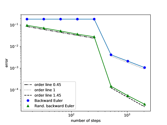
Figure 2. $L^{2}(\Omega;L^{2}(0,1))$-errors of the classical backward Euler method and scheme (6.5) for equation (8.1).

The numerical behavior of this problem is very similar to the ODE example in Section 5. The right-hand side $f$ is highly oscillating. Thus, the classical backward Euler method needs a step size smaller than $P$ in order to give an accurate numerical approximation. The randomized scheme (6.5), on the other hand, yields much better approximations of the solution for larger values of the step size.

In our numerical test displayed in Figure 2, we considered $R=10$ and $\tilde{p}=4$ in (8.2), $P=2^{-9}$ and step sizes $k=2^{n}$ with $n\in\{4,\dots,11\}$. To approximate the $L^{2}(\Omega;L^{2}(0,1))$-norm of the error we used $200$ Monte Carlo iterations. Since we are only interested in demonstrating the temporal convergence, we use a fixed finite element space with $500$ degrees of freedom based on a uniform mesh in order to keep the spatial error on a negligible level for all considered temporal step sizes. For the implementation we used the finite element software package FEniCS [31].

The results are well comparable to the results for the ODE example in Section 5. When the step size is larger than the value $P$, we can recognize a convergence rate of $0.45$ for the randomized scheme. On the other hand, the error of the classical backward Euler method does not decrease for these step sizes. The errors of both schemes improve significantly when the step size is sufficiently small to resolve the oscillations. After that we see the classical rate of $1$ for the deterministic scheme and a rate of $1.45$ in our randomized scheme.

References

- [1] H. Amann. Linear and Quasilinear Parabolic Problems. Vol. I: Abstract Linear Theory, volume 89 of Monographs in Mathematics. Birkhäuser Boston, Inc., Boston, MA, 1995.
- [2] H. Amann. Compact embeddings of Sobolev and Besov spaces. Glasnik Matematicki, 35(55):161–177, 2000.
- [3] A. Andersson and R. Kruse. Mean-square convergence of the BDF2-Maruyama and backward Euler schemes for SDE satisfying a global monotonicity condition. BIT Numer. Math., 57(1):21–53, 2017.
- [4] W. Arendt and M. Duelli. Maximal -regularity for parabolic and elliptic equations on the line. J. Evol. Equ., 6(4):773–790, 2006.
- [5] C. Baiocchi and F. Brezzi. Optimal error estimates for linear parabolic problems under minimal regularity assumptions. Calcolo, 20(2):143–176, 1983.
- [6] R. E. Bank and H. Yserentant. On the -stability of the -projection onto finite element spaces. Numer. Math., 126(2):361–381, 2014.
- [7] C. Carstensen. Merging the Bramble-Pasciak-Steinbach and the Crouzeix-Thomée criterion for -stability of the -projection onto finite element spaces. Math. Comp., 71(237):157–163 (electronic), 2002.
- [8] C. Carstensen. An adaptive mesh-refining algorithm allowing for an stable projection onto Courant finite element spaces. Constr. Approx., 20(4):549–564, 2004.
- [9] K. Chrysafinos and L. S. Hou. Error estimates for semidiscrete finite element approximations of linear and semilinear parabolic equations under minimal regularity assumptions. SIAM J. Numer. Anal., 40(1):282–306, 2002.
- [10] D. S. Clark. Short proof of a discrete Gronwall inequality. Discrete Appl. Math., 16(3):279–281, 1987.
- [11] M. Crouzeix and V. Thomée. The stability in and of the -projection onto finite element function spaces. Math. Comp., 48(178):521–532, 1987.
- [12] T. Daun. On the randomized solution of initial value problems. J. Complexity, 27(3-4):300–311, 2011.
- [13] M. Dindoš and V. Toma. Filippov implicit function theorem for quasi-Carathéodory functions. J. Math. Anal. Appl., 214(2):475–481, 1997.
- [14] E. Emmrich. Gewöhnliche und Operator-Differentialgleichungen. Vieweg, Wiesbaden, 2004.
- [15] E. Emmrich. Two-step BDF time discretisation of nonlinear evolution problems governed by monotone operators with strongly continuous perturbations. Comput. Methods Appl. Math., 9(1):37–62, 2009.
- [16] L. C. Evans. Partial Differential Equations. Graduate studies in mathematics ; 19. American Mathematical Society, 1998.
- [17] I. Gyöngy. On stochastic equations with respect to semimartingales. III. Stochastics, 7(4):231–254, 1982.
- [18] B. H. Haak and E. M. Ouhabaz. Maximal regularity for non-autonomous evolution equations. Math. Ann., 363(3-4):1117–1145, 2015.
- [19] S. Haber. A modified Monte-Carlo quadrature. Math. Comp., 20:361–368, 1966.
- [20] S. Haber. A modified Monte-Carlo quadrature. II. Math. Comp., 21:388–397, 1967.
- [21] W. Hackbusch. Optimal error estimates for a parabolic Galerkin method. SIAM J. Numer. Anal., 18(4):681–692, 1981.
- [22] E. Hairer and G. Wanner. Solving Ordinary Differential Equations. Vol. II: Stiff and Differential-Algebraic Problems, volume 14 of Springer Series in Computational Mathematics. Springer-Verlag, Berlin, 2010. Second revised edition, paperback.
- [23] J. K. Hale. Ordinary Differential Equations. Robert E. Krieger Publishing Co., Inc., Huntington, N.Y., second edition, 1980.
- [24] S. Heinrich and B. Milla. The randomized complexity of initial value problems. J. Complexity, 24(2):77–88, 2008.
- [25] L. S. Hou and W. Zhu. Error estimates under minimal regularity for single step finite element approximations of parabolic partial differential equations. Int. J. Numer. Anal. Model., 3(4):504–524, 2006.
- [26] A. Jentzen and A. Neuenkirch. A random Euler scheme for Carathéodory differential equations. J. Comput. Appl. Math., 224(1):346–359, 2009.
- [27] B. Z. Kacewicz. Optimal solution of ordinary differential equations. J. Complexity, 3(4):451–465, 1987.
- [28] B. Z. Kacewicz. Almost optimal solution of initial-value problems by randomized and quantum algorithms. J. Complexity, 22(5):676–690, 2006.
- [29] A. Klenke. Probability Theory. A Comprehensive Course. Springer, London, 2nd ed. edition, 2014.
- [30] R. Kruse and Y. Wu. Error analysis of randomized Runge-Kutta methods for differential equations with time-irregular coefficients. Comput. Methods Appl. Math., 17(3):479–498, 2017.
- [31] A. Logg, K.-A. Mardal, and G. N. Wells. Automated Solution of Differential Equations by the Finite Element Method: The FEniCS book. Lecture Notes in Computational Science and Engineering; 84. Springer, Berlin, Heidelberg, 2012 edition, 2012.
- [32] A. Lunardi. Analytic Semigroups and Optimal Regularity in Parabolic Problems. Birkhäuser, Basel, 1995.
- [33] D. Meidner and B. Vexler. Optimal error estimates for fully discrete Galerkin approximations of semilinear parabolic equations. ArXiv preprint, arXiv:1707.07889v1, 2017.
- [34] E. Novak. Deterministic and Stochastic Error Bounds in Numerical Analysis, volume 1349 of Lecture Notes in Mathematics. Springer-Verlag, Berlin, 1988.
- [35] A. Ostermann and M. Thalhammer. Convergence of Runge-Kutta methods for nonlinear parabolic equations. Appl. Numer. Math., 42(1-3):367–380, 2002. Ninth Seminar on Numerical Solution of Differential and Differential-Algebraic Equations (Halle, 2000).
- [36] A. Prothero and A. Robinson. On the stability and accuracy of one-step methods for solving stiff systems of ordinary differential equations. Math. Comp., 28:145–162, 1974.
- [37] T. Roubíček. Nonlinear Partial Differential Equations with Applications, volume 153 of International Series of Numerical Mathematics. Birkhäuser/Springer Basel AG, Basel, second edition, 2013.
- [38] G. Stengle. Numerical methods for systems with measurable coefficients. Appl. Math. Lett., 3(4):25–29, 1990.
- [39] G. Stengle. Error analysis of a randomized numerical method. Numer. Math., 70(1):119–128, 1995.
- [40] J. F. Traub, G. W. Wasilkowski, and H. Woźniakowski. Information-Based Complexity. Computer Science and Scientific Computing. Academic Press, Inc., Boston, MA, 1988. With contributions by A. G. Werschulz and T. Boult.
- [41] H. Triebel. Interpolation Theory, Function Spaces, Differential Operators. North-Holland Publishing Company, Amsterdam-New York, 1978.
- [42] E. Zeidler. Nonlinear Functional Analysis and its Applications. 2/A, Linear Monotone Operators. Springer-Verlag, New York, 1990.
- [43] E. Zeidler. Nonlinear Functional Analysis and its Applications. 2/B, Nonlinear Monotone Operators. Springer-Verlag, New York, 1990.