Fairy circle landscapes under the sea
Short-scale interactions yield large-scale vegetation patterns that, in turn, shape ecosystem function across landscapes. Fairy circles, which are circular patches bare of vegetation within otherwise continuous landscapes, are characteristic features of semiarid grasslands. We report the occurrence of submarine fairy circle seascapes in seagrass meadows and propose a simple model that reproduces the diversity of seascapes observed in these ecosystems as emerging from plant interactions within the meadow. These seascapes include two extreme cases, a continuous meadow and a bare landscape, along with intermediate states that range from the occurrence of persistent but isolated fairy circles, or solitons, to seascapes with multiple fairy circles, banded vegetation, and ”leopard skin” patterns consisting of bare seascapes patterns consisting of bare seascapes dotted with plant patches. The model predicts that these intermediate seascapes extending across kilometers emerge as a consequence of local demographic imbalances along with facilitative and competitive interactions among the plants with a characteristic spatial scale of 20 to 30 m, consistent with known drivers of seagrass performance. The model, which can be extended to clonal growth plants in other landscapes showing fairy rings, reveals that the different seascapes observed hold diagnostic power as to the proximity of seagrass meadows to extinction points that can be used to identify ecosystems at risks.
INTRODUCTION
The spatial organization of vegetation landscapes is a key factor in assessment of ecosystem health and functioning (?, ?, ?, ?). Spatial configurations of vegetation landscapes act as potential indicators of climatic or human forcing affecting the ecosystem (?) and determine energy and material budgets and feedbacks across space (?, ?, ?, ?). In addition, although vegetation tends to cover all available ground under favorable conditions, plant distributions can spontaneously develop spatial inhomogeneities under resource limitation, acting as ecosystem engineers that modify the fluxes of nutrients and water to improve their growth conditions (?, ?). Hence, the spatial organization of vegetation landscapes provides an indicator of the existence of stressing factors and the proximity of critical thresholds leading to irreversible losses (?, ?).
The processes conducive to different dynamics of vegetation landscapes have been assessed in habitats ranging from arid ecosystems and savannahs to forests and wetlands (?, ?, ?). The most striking patterns have been reported in drylands, where competition for water leads to self-organized vegetation patchiness (?, ?, ?, ?, ?), including the appearance of the so-called fairy circles, whose origin has stirred significant controversy (?, ?, ?, ?, ?). These are bare circular patches surrounded by grass, which appear, for example, in regions of the grassy deserts of Namibia (?) and Australia (?) and have been used as a basis to formulate a theory of self-organization of vegetation landscapes in water-limited ecosystems.
Although self-organized patchiness and pattern formation are well documented in terrestrial ecosystems, their occurrence in marine environments has attracted much less attention. Fairy circleâ like structures have been reported in seagrass meadows, such as Mediterranean Posidonia ocanica (?, ?) and Zostera marina in the Danish Kattegat (?). Complex landscapes, such as bare seascapes dotted with plant patches, termed ”leopard skin” (?), and stripped vegetation patterns (?, ?), have also been studied. However, inspection of satellite images and side-scan cartography reveals that complex seascapes are abundant in meadows of P. ocanica, suggesting that self-organized submarine vegetation patterns may be prevalent but have remained thus far largely hidden under the sea. Obviously, the mechanisms responsible for the formation of these submarine fairy circle landscapes must be necessarily different than those operating in water-limited ecosystems on land (?, ?, ?). Although there are some hypotheses of possible mechanisms in several marine ecosystems (?, ?, ?, ?), there is only a partial understanding of the phenomenon in P. ocanica meadows.
With a global distribution along the shorelines of all continents except Antarctica, seagrass meadows are valuable ecosystems that provide valuable ecosystem services (?); but they rank among the most threatened ecosystems globally (?). P. oceanica is the dominant seagrass in the Mediterranean Sea, where it forms underwater meadows that support great biodiversity, are a site of intense CO2 sequestration, and offer shoreline protection (?, ?). Unfortunately, this ecosystem is affected by multiple anthropogenic impacts, including reduced water quality and physical impacts, that have led to a loss of per year over the past 50 years (?). Although P. oceanica is a strongly clonal plant propagating through rhizome growth, its very slow horizontal spread of a few centimeters per year implies that losses are essentially irreversible over managerial time scales (?).
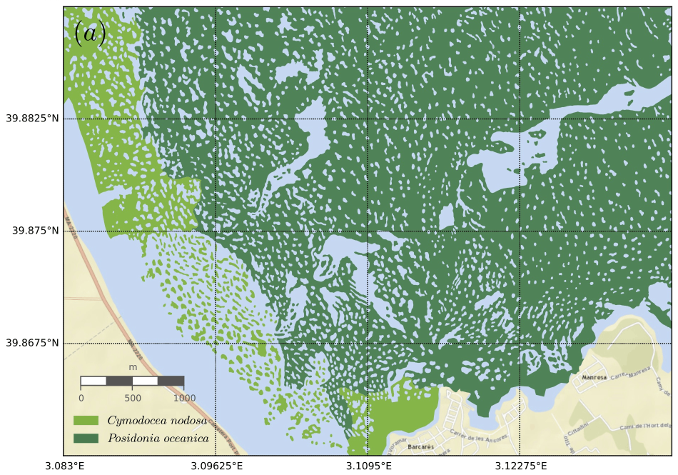
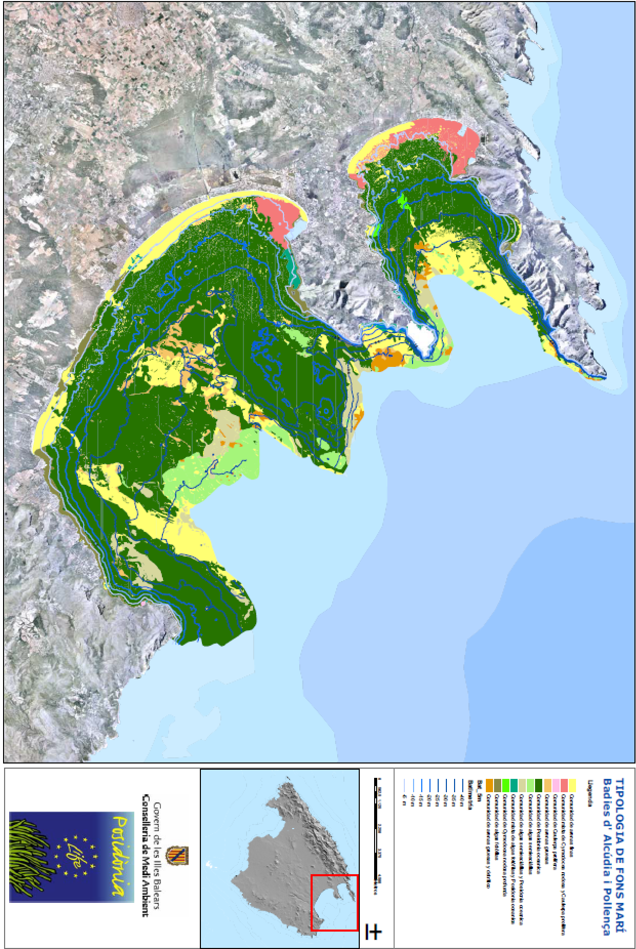
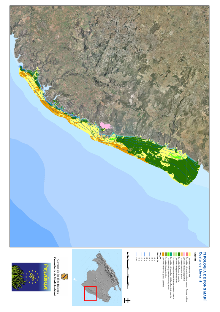
Here, we report that inspection of side-scan sonar cartography of seagrass meadows (P. oceanica and Cymodocea nodosa) in Mallorca Island (Western Mediterranean) reveals that vegetation patterns of holes and spots spanning over many kilometers are prevalent along the coastline of the Balearic Islands (see Fig. 1a) (?). We also present a simple, parsimonious model of clonal plant growth yielding self-organized submarine vegetation patterns that encompass the diversity of seascapes observed.
RESULTS
Sintes et al. (?, ?) developed a model, based on a limited set of simple rules underpinning clonal growth, successfully reproducing seagrass growth: First, the growing apex of seagrass rhizomes elongates in a fixed horizontal direction with a velocity , leaving new shoots behind, which are separated along the rhizome by a typical distance . Second, the growing apex develops new branches at a rate , with these branches elongating into a horizontal direction at an angle from the original rhizome. Living shoots have a typical lifetime, depending on external factors and the presence of neighboring shoots, resulting in a per capita mortality rate . If at a given position, the density of shoots will increase locally. The typical value of each parameter is a characteristic feature of each species with some variability driven by genetic and environmental conditions (?).
We have scaled up this model (originally conceived to describe patch development) to landscape scale by coarse-graining it to describe the dynamics of the shoot, , and apex, , densities. Total shoot density , is calculated as the sum of shoots and apices growing in all directions. This model, which we call the â œAdvection-Branching-Deathâ (ABD) model, includes rhizome growth in different directions, contributions from rhizome branching, and shoot death. Shoot mortality rates are density-dependent as well as dependent on environmental factors (for example, resource availability). More specifically, three terms contribute to the total mortality
| (1) |
On the one hand, the intrinsic mortality rate, , of an individual shoot at a particular position in the landscape depends on environmental factors, and on the other hand, on two density-dependent terms: local saturation and nonlocal interaction.The saturation term is nonlinear and prevents an unlimited growth, increasing mortality locally when the density increases excessively. The strength b of this density-dependent term reflects the environmental carrying capacity, determining the maximum density in the meadow. Nonlocal interactions are included through an integral term accounting for the interaction of shoots at positionâ r with those in a neighborhood weighted by the kernel . Through nonlocal interactions, the abundance of shoots in a place can affect the growth in a neighborhood. The model therefore includes two essential components to yield self-organization: nonlinearity and spatial interaction.
The three terms in Eq. 1 are consistent with the current functional understanding of seagrass meadows. The intrinsic mortality rate of individual shoots, determining , depends on external factors such as temperature and irradiance regimes (?). Local density dependence results from self-shading, determining the maximum density of shoots for a given plant size (?) and the general decline in seagrass density and biomass with depth (?), as well as local depletion of other resources, such as CO2, which is depleted during daytime in dense meadows (?). Nonlocal interactions integrate a number of facilitative and competitive mechanisms. Facilitative interactions arise, for instance, in the form of stress amelioration, when the presence of neighboring plants dissipates wave energy, which may prevent shoot removal from scouring of waves within the meadow (?) and contributes to stabilize and trap sediments (?). Facilitation has been argued to play a role in shaping seagrass landscapes (?, ?). Negative interactions appear, for instance, as a result of anaerobic microbial decomposition in dense meadows, which leads to diffusing sulfide fronts that spread mortality, leading to the appearance of fairy rings (?). Competition can arise also from depletion of nutrients from the flow by plants up-current (?) or of other diffusing resources, such as CO2.
Hence, existing evidence suggests intraspecific facilitation and competitive nonlocal interaction whose precise ranges are difficult to determine. As a result of these interactions, the meadow can self-organize enhancing facilitative effects and diminishing competition, altering the environment to yield more favorable growth conditions.
We consider a kernel with two terms of Gaussian shape
| (2) |
where is the strength of the competitive interaction with width , and is the strength of facilitation with width , where the widths of the Gaussians correspond to the spatial extension of the interactions. Note that we should have to guarantee positive mortality. For simplicity, in the following, we take . As a result of the two Gaussians with different widths and signs, the kernel has the shape of an inverted Mexican hat, and the interaction is stronger at short distances, decaying very fast with .
Competition or facilitation may dominate at shorter or longer distances depending on the values of and . On general grounds, the main effect of facilitation is to permit the coexistence of the populated and unpopulated homogeneous states, whereas nonlocal competition is one of the mechanisms responsible for the spontaneous formation of regular patterns, either on itself (?) or acting together with the facilitative interaction (?). Thus, observation of spatial patterns suggests the existence of nonlocal competitive interactions. Selecting results in a kernel that is weakly competitive at large distances, yielding to a suitable nonlocal interaction for pattern formation (see the Supplementary Materials) (?). The main nonlocal interaction terms (, , , ) can be inferred from the comparison of numerical simulations and observed patterns, whereas seagrass growth parameters are largely known [see the study by Sintes et al. (?) and references therein].
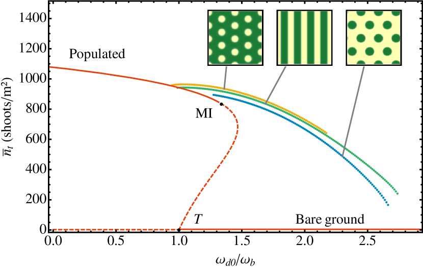
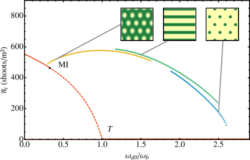
The ABD model yields a great diversity of complex spatial patterns emerging at different parameter regions, including nonlinear phenomena resulting in the coexistence of different solutions, which are shown in Fig. 2 for the case of constant and . When mortality is high (), the only possible solution is bare soil, the unpopulated solution. Decreasing the mortality (or increasing branching rate), the unpopulated solutions become unstable at a threshold . Below this mortality, any small nonzero density will grow to form a meadow. If mortality is much smaller than the branching rate, , the vegetation will uniformly cover all the available space. Thus, there are two extreme homogeneous stable states: a uniform, continuous meadow () and bare seafloor, with no vegetation (), as it is shown in Fig. 2 (red solid lines). The parameter values that better reproduce the observed patterns of P. oceanica meadows correspond to a kernel that, although competition extends farther, is overall facilitative. As a result, the transition (T) from bare soil to the populated solution is subcritical, so that there is a mortality range in which both populated and unpopulated solutions coexist (Fig. 2). Competition between shoots can destabilize the populated solution, leading to patterns, whereas the homogeneous states are the only possible solutions in the absence of nonlocal interactions. Therefore, the presence of fairy circle landscapes in seagrass meadows is indirect evidence of nonlocal negative interactions.
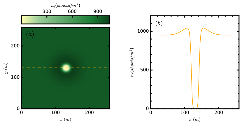
A linear stability analysis of the homogeneous populated solution reveals that it undergoes a finite wavelength instability, also known as Turing (?) or modulation instability (MI), at a critical value of mortality rate (in Fig. 2, ), leading to the emergence of complex spatial patterns. Above this mortality, any small perturbation to the homogeneous meadow is enough to trigger a feedback process driving the vegetation to form an inhomogeneous pattern. Different spatial structures are possible. As mortality rate increases, possible patterns shift from negative hexagons (holes arranged in a hexagonal pattern), to stripes, and to positive hexagons (spots of vegetation arranged in a hexagonal pattern), as expected from the general theory of pattern formation (?, ?). Each solution is stable in a different region of parameter space, and two different solutions can be simultaneously stable for the same value of the mortality, a coexistence between solutions that would give rise to hysteresis. In particular, negative hexagons coexist with the homogeneous populated solution in a mortality range below . In part of this region, a single bare hole embedded in a dense meadow (Fig. 3), known as dissipative soliton (?), which is the submarine analog of a terrestrial fairy circle, can be stable (?, ?). Many of the bare circles visible in the coasts of Mallorca and the Adriatic Sea (Fig. 1) can be identified with dissipative solitons.
Thus, our model is able to reproduce and to facilitate understanding of the nonlinear behavior, leading to the emergence of dynamic complex landscape patterns in seagrass meadows. The spatial scale of real patterns is mainly related to the range of the competing interaction . An estimation of the length scale of the observed patterns can be obtained using the Fourier spectrum (see the Supplementary Materials) of images such as Fig. 1a). It is not always possible to obtain a precise estimate of this length scale, because often, patterns are not regular enough, although local hexagonal ordering can be appreciated in the more regular regions. In these regions, one can identify in the Fourier spectrum a typical periodicity of (see the Supplementary Materials). Choosing , the critical wavelength at the MI threshold (see the Supplementary Materials) fits this observed characteristic length, and simultaneously, a typical hole size of about 30 is also correctly reproduced. This result allows us to conjecture the existence of a competitive interaction with a range of around 20 to 30 , whose specific nature is not yet known. In addition to their local contribution, the competition for natural resources (for example, dissolved inorganic nutrients or CO2) and the interactions mediated by toxic compounds, such as sulfide, which is accumulated in the soil (?), are expected to contribute to nonlocal competitive interactions. Other hypotheses include interaction through hydrodynamics, which may modify the sedimentary delivery of nutrients.
The time scales for the landscape dynamics captured by the model are long, encompassing decades to millennia (movies S1 to S5 and the Supplementary Materials), depending on the characteristic demographic time scales of the species. For instance, P. oceanica clones are long-lived organisms, with clones living tens of thousands of years (?) and forming meadows over centuries to millennia (?, ?), whereas C. nodosa grows much faster and can form meadows over decades to centuries (?). Hence, the dynamics conducive to formation of complex landscape patterns and the transition between them are too slow to be observed empirically and can be grasped only through a modeling approach, such as the one developed here (movies S1 to S6), with parameter values properly constrained by present-day observations.
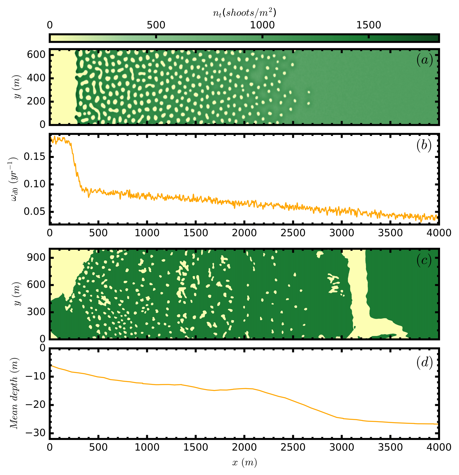
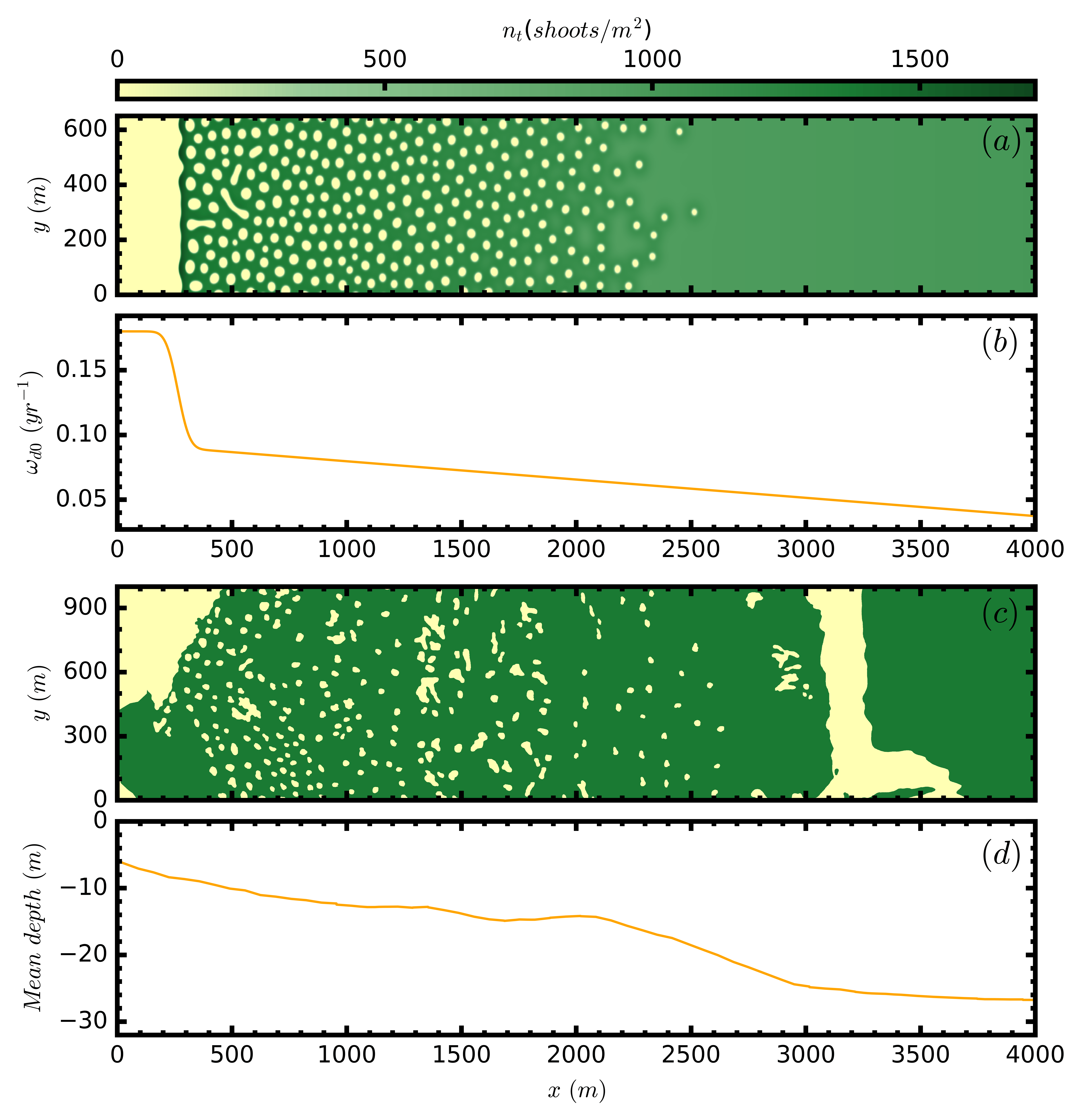
In addition to providing qualitative understanding of how demographic imbalances affect the spatial configuration of seagrass meadows, the model proposed provides a remarkable, given its parsimony, description of observed patterns in seagrass meadows (Fig. 4). Two additional model components are needed to reproduce observed density patterns: a decline in mortality rate, , with the distance from the coast, , and a spatial random noise term that mimics irregular spatial variability of the parameters. Simulations in small systems and under ideal conditions (that is, in the absence of noise) may yield perfectly periodic patterns (insets in Fig. 2), whereas simulations in large domains, including noise, better resemble observed patterns (Figs. 4 and 5, movies S4 to S6, and the Supplementary Materials).
The increase in area coverage from the shore toward moderate depths is characteristic of P. oceanica meadows (Fig. 4c) [as is also the its decrease and disappearance toward deep waters; (?)]. This indicates high mortality rates in shallow, nearshore waters, which could be attributed to scouring by waves, leading to the unpopulated model solution in waters shallower than the upslope limit of the seagrass, and low mortality rates in moderately deeper waters, allowing the formation of stable homogeneous meadows. A smooth decline in mortality with depth should then lead to complex spatial patterns at intermediate depths, where the homogeneous solution is unstable (see Fig. 2). Including such decline in mortality (Fig. 4b) with added noise (see the Supplementary Materials), the resulting patterns (Fig. 4a) accurately reproduce observed features in P. oceanica meadows (Fig. 4c), such as more elongated vegetation gaps near the shore and scattered gaps close to the homogeneous meadow. The transition from bare soil to patterns with elongated gaps signals that this region experiences a steep mortality decrease from very high to moderate values where hexagons begin to be unstable with respect to stripes. Scattered gaps are well reproduced close to the homogeneous meadow, in a mortality range where hexagonal gap patterns coexist with the homogeneous populated state (see Fig. 2) and dissipative solitons (fairy circles) can form. Further downslope, the homogeneous meadow prevails.
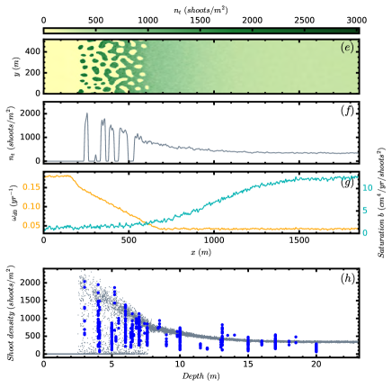
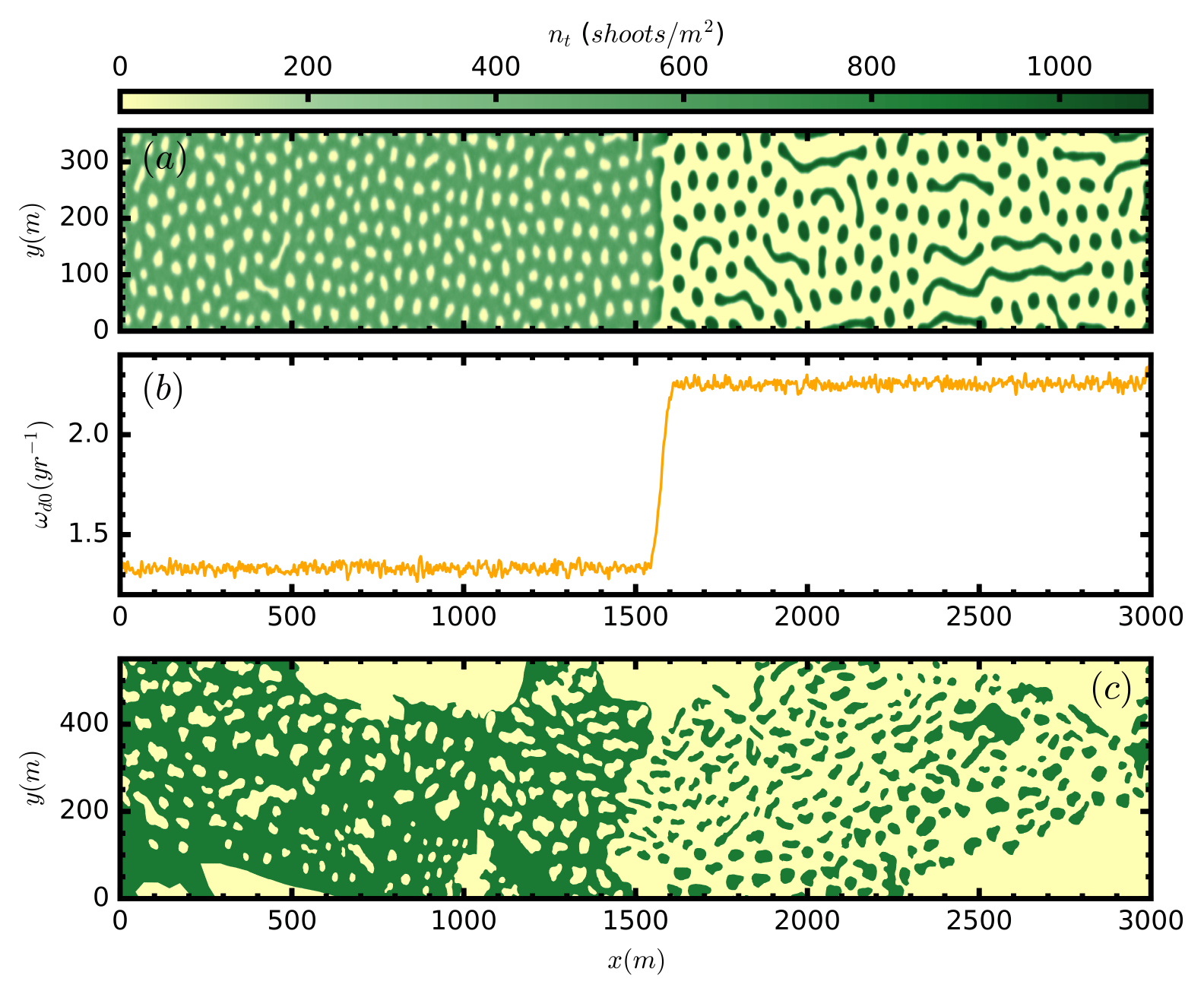
The model also reproduces the decline of shoot density and its variability with depth observed in meadows along the littoral of the Balearic Islands (Fig. 4h). Shoot density was measured by scuba divers at random positions in the meadows without previous knowledge of their spatial distribution. The results consistently showed low shoot density variability at depths 10 compared to high variability at shallower depths ( 10 ), ranging from close to 0 to 2000 , a variability much larger than that in deeper regions (thick blue dots Fig. 4h). Our model suggests that high shoot density variability in shallow waters is a consequence of the presence of complex spatial patterns near the coast. Simulations using noisy and depth-dependent mortality and carrying capacity, (see Fig. 4g), account for the decrease in shoot density with depth and generate patterns of shoot density that capture the dispersion of the density close to the coast where patterns form (Fig. 4 e to h, and movie S5). The model also reproduces complex patterns in meadows of C. nodosa, such as the transition from holes to patches observed in one of the meadows (Figs. 1, and 5c). Because this transition occurs parallel to the coast, that is, at a uniform depth, we inferred this pattern to be derived from a sudden increase in the mortality rate along the shore (see Fig. 5b). The resulting simulated pattern (Fig. 5a) reproduces very well the observed features of the real meadow, further confirming that the complex seascape of fairy circle patterns observed in Mediterranean seagrass meadows can be reproduced parsimoniously as a consequence of variability in the seagrass demographic balance caused by spatial interaction and nonlinearity.
DISCUSSION
We have demonstrated that complex landscape patterns, such as those dotted by fairy circles characteristic of arid grasslands, are also common features of seagrass seascapes in the Mediterranean and have also been reported in seagrass meadows elsewhere (?, ?, ?, ?). The parsimonious model developed here demonstrates that fairy circle seascapes emerge as consequences of nonlinearity and spatial interactions in seagrass meadows at critical levels of demographic imbalances, typically met in relatively shallow nearshore areas of seagrass meadows. In contrast, comparatively low mortality rates in deeper areas lead to a prevalence of stable continuous meadows toward the deeper ranges of seagrass meadows. The model developed here, based on simple inherent growth traits of the seagrass species and variable mortality due to nonlocal interaction and nonlinearity, is able to reproduce the range of complex landscape configurations, including striped, hexagon, and soliton- dominated landscapes encountered between the bare sediments and continuous meadow end members for these landscapes. The model results are robust enough as to allow inferences on the demographic status of the meadows on the basis of observed landscape configurations. In particular, positive hexagons signal the proximity of tipping points where further increase in seagrass mortality relative to growth may lead to catastrophic loss of seagrass meadows (?, ?). Because seagrass ecosystems rank among the most threatened ecosystems globally (?), the capacity to diagnose the proximity of seagrass meadows to tipping points for catastrophic loss based on landscape configurations provides a tool to guide conservation measures aimed at preventing further losses.
MATERIALS AND METHODS
Derivation of the Advection-Branching-Death model
Focusing on the three main mechanisms involved in the growth of clonal plants, namely, apices’ linear growth, branching, and death, we developed a set of partial differential equations (PDEs; or, more precisely, integro-differential equations) for the density of shoots and apices. These mechanisms were identified and implemented in a previous model, which focused on individual shoots (?, ?). Here, we formulated these mechanisms in terms of upscaled continuous densities, thus allowing for the description of much larger spatial and temporal scales. The spatial density of shoots at position of the sea bottom at time is , and the density of apices growing in the direction given by the angle is . Note that the magnitude of the apices’ growth velocity is assumed constant, and a growth velocity vector can be written as . The total density of shoots, , considering for simplicity that an apex is carrying a shoot, is the sum of shoots and apices growing in all directions, .
Two PDEs describing the evolution of the densities of shoots and apices can be derived in terms of the contributions of the three growth mechanisms to the number of shoots in an infinitesimal surface. First, the number of apices growing in direction at in an infinitesimal surface of area located at will be the sum of two contributions: (i) the apices that remain alive coming from because of rhizome elongation and (ii) new apices that appear because of branching from directions of growth and , which are the only directions contributing to the growth in direction . is the branching angle. Note that those apices that go away due to rhizome elongation are contributing to position . Then, we obtain
| (3) |
where and are branching and death rates, respectively. Making a Taylor expansion of Eq. Derivation of the Advection-Branching-Death model and neglecting second-order terms and higher, we obtain
| (4) |
Rewriting Eq. Derivation of the Advection-Branching-Death model, we obtain the PDE that describes the growth of apices in the direction
| (5) |
where .
The same procedure can be used to obtain the equation for the
shoot density. The first contribution is the shoots that remain
alive at the same position, and the second contribution is due
to the apices that survive and go away in any direction leaving
a shoot behind
| (6) |
where is the distance between shoots. Using the Taylor expansion and keeping first-order terms only, we have
| (7) |
which leads to the PDE for the shoot population density
| (8) |
The time evolution of a meadow can then be described by two coupled PDEs, Eqs. Derivation of the Advection-Branching-Death model and 8, one for each population density. We name this set of two equations the ABD model. The first term in Eqs. Derivation of the Advection-Branching-Death model and 8 corresponds to death of shoots and apices. The same death rate is considered. The second term in Eq. Derivation of the Advection-Branching-Death model is an advection in the direction of the elongation of the rhizome, describing the movement of the apices. The last term in Eq. Derivation of the Advection-Branching-Death model corresponds to the branching process. Finally, the second term in Eq. 8 accounts for the shoots left behind by the apices. The death rate is given by
| (9) |
| (10) |
where for simplicity and . Both interaction terms in Eq. 10 are considered to have a Gaussian shape , where . Other kernels have been considered in the literature in different contexts (?), although qualitatively, the pattern formation feature does not depend strongly on the precise shape of the kernel (?, ?), provided it decays faster or equal than exponential (?). Figure S5 shows the form of the kernel used in this work. Thus, the interaction is stronger for short distances and decreases exponentially fast with . Because is normalized to 1, if (), then the interaction is overall competitive (facilitative). Depending on the values of and , competition or facilitation may dominate at short or long distances. The term be expanded for low densities as , leading to the usual nonlocal term in Lotka-Volterraâ like models (?). The exponential has been introduced to saturate the interaction strength for high densities, such that the mortality rate cannot become negative because of the facilitative interaction leading to the local creation of plants, which is unreal because a new shoot can be created only through the growth of the rhizomes or a branching event. For low densities, then, parameter multiplies the strength of the nonlocal interaction. However, the larger the parameter , the faster the saturation of the interaction as the density grows. Varying and , one can change the relative strength between competition and facilitation. Here, we chose a kernel that is facilitative at short ranges and competitive at larger scales (Fig. S5).
References and Notes
- 1. M. Rietkerk, S. C. Dekker, P. C. de Ruiter, J. van de Koppel, Self-organized patchiness and catastrophic shifts in ecosystems. Science 305, 1926–1929 (2004).
- 2. N. Barbier, P. Couteron, J. Lejoly, V. Deblauwe, O. Lejeune, Self-organized vegetation patterning as a fingerprint of climate and human impact on semi-arid ecosystems. Journal of Ecology 94, 537–547 (2006).
- 3. R. Sole, J. Bascompte, Self-Organization in Complex Ecosystems (Princeton University Press, 2006).
- 4. M. Rietkerk, J. Van de Koppel, Regular pattern formation in real ecosystems. Trends in Ecology & Evolution 23, 169–175 (2008).
- 5. R. Lefever, O. Lejeune, On the origin of tiger bush. Bulletin of Mathematical Biology 59, 263–294 (1997).
- 6. J. Thiery, J.-M. d’Herbes, C. Valentin, A model simulating the genesis of banded vegetation patterns in Niger. Journal of Ecology pp. 497–507 (1995).
- 7. E. Gilad, J. von Hardenberg, A. Provenzale, M. Shachak, E. Meron, A mathematical model of plants as ecosystem engineers. Journal of Theoretical Biology 244, 680 - 691 (2007).
- 8. M. Scheffer, et al., Early-warning signals for critical transitions. Nature 461, 53–9 (2009).
- 9. J. Von Hardenberg, E. Meron, M. Shachak, Y. Zarmi, Diversity of vegetation patterns and desertification. Physical Review Letters 87, 198101 (2001).
- 10. E. Meron, E. Gilad, J. von Hardenberg, M. Shachak, Y. Zarmi, Vegetation patterns along a rainfall gradient. Chaos, Solitons & Fractals 19, 367–376 (2004).
- 11. E. Meron, Pattern-formation approach to modelling spatially extended ecosystems. Ecological Modelling 234, 70–82 (2012).
- 12. C. Fernandez-Oto, M. Tlidi, D. Escaff, M. Clerc, Strong interaction between plants induces circular barren patches: fairy circles. Philosophical Transactions of the Royal Society of London A: Mathematical, Physical and Engineering Sciences 372, 20140009 (2014).
- 13. T. M. Scanlon, K. K. Caylor, S. A. Levin, I. Rodriguez-Iturbe, Positive feedbacks promote power-law clustering on Kalahari vegetation. Nature 449, 209 (2007).
- 14. M. D. Cramer, N. N. Barger, Are Namibian fairy circles the consequence of self-organizing spatial vegetation patterning? PloS one 8, e70876 (2013).
- 15. N. Juergens, The biological underpinnings of Namib desert fairy circles. Science 339, 1618–1621 (2013).
- 16. S. Getzin, et al., Discovery of fairy circles in Australia supports self-organization theory. Proceedings of the National Academy of Sciences 113, 3551–3556 (2016).
- 17. C. E. Tarnita, et al., A theoretical foundation for multi-scale regular vegetation patterns. Nature 541, 398–401 (2017).
- 18. V. Pasqualini, C. Pergent-Martini, G. Pergent, Environmental impact identification along the Corsican coast (Mediterranean sea) using image processing. Aquatic Botany 65, 311–320 (1999).
- 19. M. Bonacorsi, C. Pergent-Martini, N. Breand, G. Pergent, Is Posidonia oceanica regression a general feature in the Mediterranean Sea? Mediterranean Marine Science 14, 193–203 (2013).
- 20. J. Borum, et al., Eelgrass fairy rings: sulfide as inhibiting agent. Marine Biology 161, 351–358 (2014).
- 21. C. Den Hartog, The dynamic aspect in the ecology of seagrass communities. Thalassia Jugoslavica 7, 101–1127 (1971).
- 22. M. Frederiksen, D. Krause-Jensen, M. Holmer, J. S. Laursen, Spatial and temporal variation in eelgrass (Zostera marina) landscapes: influence of physical setting. Aquatic Botany 78, 147–165 (2004).
- 23. T. Van Der Heide, et al., Spatial self-organized patterning in seagrasses along a depth gradient of an intertidal ecosystem. Ecology 91, 362–369 (2010).
- 24. N. Marbà, C. M. Duarte, Coupling of seagrass (Cymodocea nodosa) patch dynamics to subaqueous dune migration. Journal of Ecology pp. 381–389 (1995).
- 25. N. Marbà, J. Cebrian, S. Enriquez, C. M. Duarte, Migration of large-scale subaqueous bedforms measured with seagrasses (Cymodocea nodosa) as tracers. Limnology and Oceanography 39, 126–133 (1994).
- 26. M. J. Christianen, et al., Habitat collapse due to overgrazing threatens turtle conservation in marine protected areas. Proceedings of the Royal Society of London B: Biological Sciences 281, 20132890 (2014).
- 27. M. A. Hemminga, C. M. Duarte, Seagrass ecology (Cambridge University Press, 2000).
- 28. M. Waycott, et al., Accelerating loss of seagrasses across the globe threatens coastal ecosystems. Proceedings of the National Academy of Sciences 106, 12377–12381 (2009).
- 29. C. M. Duarte, T. Sintes, N. Marbà, Assessing the CO2 capture potential of seagrass restoration projects. Journal of Applied Ecology 50, 1341–1349 (2013).
- 30. N. Marbà, E. Díaz-Almela, C. M. Duarte, Mediterranean seagrass (Posidonia oceanica) loss between 1842 and 2009. Biological Conservation 176, 183–190 (2014).
- 31. We have used side-scan sonar cartography produced by the LIFE Posidonia project http://lifeposidonia.caib.es.
- 32. T. Sintes, N. Marbà, C. M. Duarte, G. A. Kendrick, Nonlinear processes in seagrass colonisation explained by simple clonal growth rules. Oikos 108, 165–175 (2005).
- 33. T. Sintes, N. Marbà, C. M. Duarte, Modeling nonlinear seagrass clonal growth: assessing the efficiency of space occupation across the seagrass flora. Estuaries and Coasts 29, 72–80 (2006).
- 34. C. M. Duarte, Temporal biomass variability and production/biomass relationships of seagrass communities. Marine Ecology Progress Series. Oldendorf 51, 269–276 (1989).
- 35. C. M. Duarte, J. Kalff, Latitudinal influences on the depths of maximum colonization and maximum biomass of submerged angiosperms in lakes. Canadian Journal of Fisheries and Aquatic Sciences 44, 1759–1764 (1987).
- 36. C. M. Duarte, Seagrass depth limits. Aquatic Botany 40, 363–377 (1991).
- 37. O. Invers, J. Romero, M. Pérez, Effects of ph on seagrass photosynthesis: a laboratory and field assessment. Aquatic Botany 59, 185–194 (1997).
- 38. D. Patriquin, â œmigrationâ of blowouts in seagrass beds at barbados and carriacou, west indies, and its ecological and geological implications. Aquatic Botany 1, 163–189 (1975).
- 39. J. Gutiérrez, et al., Physical ecosystem engineers and the functioning of estuaries and coasts. Treatise on Estuarine and Coastal Science pp. 53–81 (2011).
- 40. M. S. Fonseca, M. Koehl, B. S. Kopp, Biomechanical factors contributing to self-organization in seagrass landscapes. Journal of Experimental Marine Biology and Ecology 340, 227–246 (2007).
- 41. C. Boström, E. L. Jackson, C. A. Simenstad, Seagrass landscapes and their effects on associated fauna: a review. Estuarine, Coastal and Shelf Science 68, 383–403 (2006).
- 42. C. D. Cornelisen, F. I. Thomas, Water flow enhances ammonium and nitrate uptake in a seagrass community. Marine Ecology Progress Series 312, 1–13 (2006).
- 43. R. Martínez-García, J. M. Calabrese, E. Hernández-García, C. López, Vegetation pattern formation in semiarid systems without facilitative mechanisms. Geophysical Research Letters 40, 6143–6147 (2013).
- 44. D. Walgraef, Spatio-temporal pattern formation (Springer-Verlag, New York, 1997).
- 45. K. Gowda, H. Riecke, M. Silber, Transitions between patterned states in vegetation models for semiarid ecosystems. Physical Review E 89, 022701 (2015).
- 46. N. Akhmediev, A. Ankiewicz, Dissipative Solitons: From Optics to Biology and Medicine (Springer-Verlag, 2008).
- 47. P. Woods, A. Champneys, Heteroclinic tangles and homoclinic snaking in the unfolding of a degenerate reversible Hamiltonian-Hopf bifurcation. Physica D 129, 147 (1999).
- 48. P. Coullet, C. Riera, C. Tresser, Stable static localized structures in one dimension. Physical Review Letters 84, 3069 (2000).
- 49. S. Arnaud-Haond, et al., Implications of extreme life span in clonal organisms: millenary clones in meadows of the threatened seagrass Posidonia oceanica. PLoS One 7, e30454 (2012).
- 50. C. M. Duarte, Submerged aquatic vegetation in relation to different nutrient regimes. Ophelia 41, 87–112 (1995).
- 51. G. A. Kendrick, N. Marbà, C. M. Duarte, Modelling formation of complex topography by the seagrass Posidonia oceanica. Estuarine, Coastal and Shelf Science 65, 717–725 (2005).
- 52. K. Siteur, et al., Beyond turing: The response of patterned ecosystems to environmental change. Ecological Complexity 20, 81–96 (2014).
- 53. S. Pigolotti, C. López, E. Hernández-García, K. H. Andersen, How Gaussian competition leads to lumpy or uniform species distributions. Theoretical Ecology 3, 89 (2010).
- 54. P. Colet, M. A. Matías, L. Gelens, D. Gomila, Formation of localized structures in bistable systems through nonlocal spatial coupling. I. General framework. Physical Review E 89, 012914 (2014).
- 55. L. Gelens, M. A. Matías, D. Gomila, T. Dorissen, P. Colet, Formation of localized structures in bistable systems through nonlocal spatial coupling. II. The nonlocal Ginzburg-Landau equation. Physical Review E 89, 012915 (2014).
- 56. C. Fernandez-Oto, M. Clerc, D. Escaff, M. Tlidi, Strong nonlocal coupling stabilizes localized structures: An analysis based on front dynamics. Physical Review Letters 110, 174101 (2013).
- 57. S. Pigolotti, C. López, E. Hernández-García, Species clustering in competitive Lotka-Volterra models. Physical Review Letters 98, 258101 (2007).
- 58. R. Montagne, E. Hernández-García, A. Amengual, M. San Miguel, Wound-up phase turbulence in the complex Ginzburg-Landau equation. Physical Review E 56, 151 (1997).
Acknowledgements:
-
•
We acknowledge helpful discussions with C. López. Funding: D.R.-R., D.G., T.S., E.H.-G., and N.M. acknowledge financial support from AEI/FEDER [Agencia Estatal de InvestigacioÌ n/Fondo Europeo de Desarrollo Regional, European Union (EU)] (FIS2015-63628-C2-1-R, FIS2015-63628-C2-2-R, and CGL2015-71809-P). C.M.D. was supported by King Abdullah University of Science and Technology through the baseline funding.
-
•
Author contributions: D.G., E.H.-G., and T.S. conceived and designed the research. D.R.-R., D.G., E.H.-G., and T.S. derived the ABD model. D.R.-R. performed the numerical simulations supervised by D.G.. N.M. and C.M.D. provided the experimental data. D.R.-R. processed and analyzed the experimental data. All authors contributed to scientific discussions and to the writing of the paper.
-
•
Competing interests: The authors declare that they have no competing interests.
-
•
Data and materials availability: All data needed to evaluate the conclusions in the paper are present in the paper and/or the Supplementary Materials. Additional data related to this paper may be requested from the authors.
SUPPLEMETNARY MATERIALS
MATERIALS AND METHODS
Homogeneous solutions and linear stability analysis
To simplify the calculations it is convenient to work with dimensionless units, such that time, space and density of shoots and apices in the new units are given by: , , and . We note that the branching rate fixes the temporal scale, the spatial scale is determined by the velocity of the rhizome elongation, and the scale of the number of shoots is determined by the saturation parameter . In the following we drop the primes from the variables and parameters expressed in the new units.
The homogeneous stationary solutions can be obtained from Eqs. Derivation of the Advection-Branching-Death model and 8 on the main text by setting the temporal and spatial derivatives equal to zero. Two solutions can be found, the trivial zero solution, which we will refer to as the unpopulated solution, and the populated solution, given by following implicit equation:
| (11) |
where . Here we consider that the density of apices is the same for all the growing directions, and therefore . We focus in the positive-density solutions. Mathematical solutions with negative density exist, but we neglect them as they have no biological meaning. We are mainly interested in the dependence of the populated solution on , that controls the external stress which the plant is exposed to. Therefore, in the following, we consider as the main control parameter. The dependence of the populated solution on is shown in the bifurcation diagrams, where the homogeneous solution is represented in red (see Fig. 2). We can distinguish two different regimes depending on the value of the ratio . When , the interaction is overall cooperative. In this case, the bifurcation from the unpopulated to the populated states (occurring at ) is subcritical, and the populated solution coexist with the unpopulated stated in a certain range of values of , as can be seen in Fig. 2. When , the interaction is overall competitive and there is no coexistence, as can be seen in Fig. S1. The populated solutions is said to be supercritical. A priory both scenarios are good candidates to reproduce the behavior of P. oceanica, however the existence of localized structures is associated to subcritical parameter sets, and this is the reason why we chose in this work.
To study the stability of the homogeneous solutions we consider perturbations of the form , . The linearized systems reads:
| (12) | |||
| (13) |
where and is a unit vector in direction . Since the advection term is periodic in [], Eqs. 12-13 are a set of linear differential equations with periodic coefficients of periodicity . Because the dependence in should be periodic, perturbations can be written in the following form:
| (14) |
| (15) |
where is the imaginary unit, and . Introducing Eqs. 14-15 in 12-13 we obtain the following set of coupled linear ordinary differential equations for the components , :
| (16) |
| (17) |
| (18) |
where .
Eqs. 16-18 describe the linear evolution of the
perturbation of the homogeneous solutions. The rsh of this
system of equations can be written in a matrix form of infinite
dimension. Truncating the matrix operator at order
(neglecting contributions with )
111This truncation is equivalent to the numerical
discretization of that has been used for the numerical
simulations. and diagonalizing numerically we find the growth
rate of perturbations with wavenumber . The
diagonalization leads to 10 eigenvalues for each . The
solution is stable if all eigenvalues have
negative real part. On the contrary, if the real part of the
eigenvalue for a given wave number becomes positive,
the homogeneous solution becomes unstable to perturbations with
the corresponding spatial periodicity, and a spatial patterns
forms (see Fig. S1).
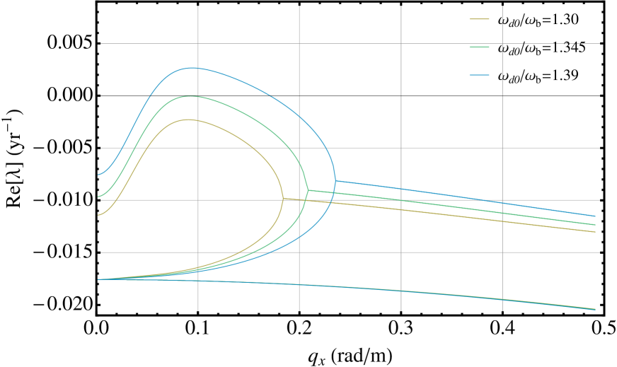
Figure S2 shows the dispersion relation of the branch of eigenvalues with largest real part. For the parameter values considered here, the first eigenvalue that become positive is a real eigenvalue with , the critical wavenumber. This is a pattern-forming instability known as Turing or modulational instability (MI).
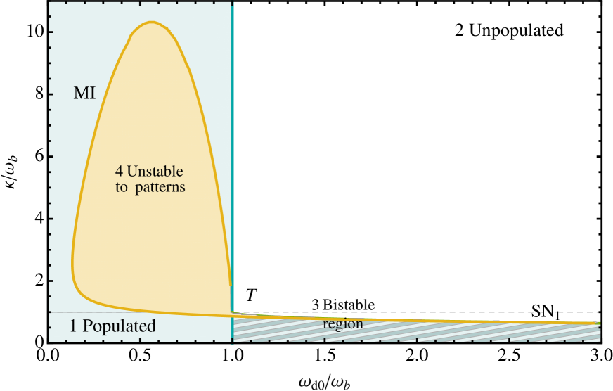
With this procedure we can determine the regions in the parameter space (, ) where the populated and unpopulated homogeneous solutions are stable or unstable. This is summarized in the phase diagram shown in Fig. S3. The unpopulated solution is stable if the branching rate is smaller than the mortality rate (region 2). If the density of shoots grows exponentially in the linear regime, and the systems goes to the populated solution. corresponds to a transcritical bifurcation indicated by T in Fig. S3.
The populated solution exist for and it is stable in blue region 1. However, if (interaction overall cooperative) the population solution extends to mortalities larger than the branching rate , and it coexists with the unpopulated solution until the saddle-node bifurcation line indicated as SN1 (shaded region 3). The populated solution is unstable to periodic patterns in the yellow region 4. Region 4 is delimited by the MI line.
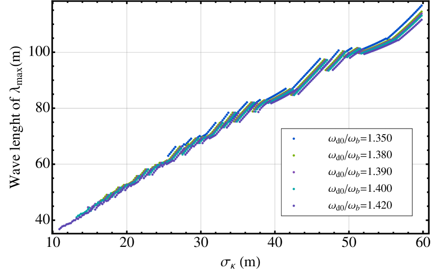
The linear stability analysis allows us to obtain the critical wavenumber of the MI, which determines the typical periodicity of the pattern () arising from the bifurcation. Fig. S4 shows the dependence of the corresponding wavelength of the wavenumber with maximum growth rate as function of the range of the competitive interaction . At the MI this wavenumber coincides with . From these results, and using the typical periodicity of real patterns (), we can find an estimation of the value of around . Although the exact number depends on the precise value of , the dependence on this parameter is small and the wavenumber is mainly determined by the value of .
Numerical simulations
Pseudospectral method
The ABD model is a system of two coupled nonlinear integro-diferential equations with partial derivatives. A pseudo-spectral method is used to integrate the time evolution of the model equations Derivation of the Advection-Branching-Death model and 8 on the main text. The model is effectively three dimensional, two spatial dimensions (, ), and one angular dimension () corresponding to the direction of growth of the apices. Since we are mainly interested in the spatial distribution of the population densities, we use the minimum number of grid points in space compatible with the branching angle. In this case, then, we consider angles multiple of , which describes well the branching angle both for P. oceanica as for C. nodosa (?, ?). This means that we describe the apices growing only in eight different directions. We have checked that increasing the number of directions does not qualitative changes the results and it considerable increases the computational needs. In practice we have then nine two-dimensional fields: one for the density of shoots and 8 for the density of apices growing in each corresponding direction. The nine fields, that depend on (, ), are coupled through the branching and the total density in the nonlocal term. We consider a square grid with and grid points and we integrate the time evolution using a pseudo-spectral method where the linear terms in Fourier space are integrated exactly, while the nonlinear terms are integrated using a second-order in time scheme described in Ref. (?).
Numerical simulations provide information about the nonlinear behavior of the system that can not be predicted by the linear stability analysis. Typical simulations start with the homogeneous solution with a superimposed small random perturbation. In stable regions of parameter space perturbations decay, and the solution remains, while in regions where the homogeneous solution is unstable, perturbations grow, and the nonlinear dynamics send the system to a different stable solution. In the region unstable to patterns, initial homogeneous solutions develop modulations that grow until a pattern forms. Different patterns appear depending on the parameters, as we can see in Fig. 2 and in Fig. S1. The regions of stability of positive and negative hexagons and stripes change with , as well as the prevalence of one over another. To study the stability of the different spatial patterns changing mortality we have performed simulations continuing . We start with an initial condition of a pattern, we add small white noise, and we change the mortality a small amount, letting the system evolve to reach a new stationary state. We use then, the final state as initial condition for the next parameter step. Repeating this procedure we can generate the stable branches shown in the bifurcation diagrams, where the average densities of each final state is plotted.
Mortality profiles
In order to introduce a mortality profile in the simulations we have to take into account two things. First we have to introduce a matrix with the values of the mortality at each position. Second, since the pseudospectral method needs periodic boundary conditions the introduced profile must be periodic, in the center the profile can have the desired shape but opposite boundaries must connect smoothly. The easiest way to produce a profile is to design it using straight lines and apply a filter to smooth out the corners. For the last step we use a diffusion operator in Fourier space. We apply the Fourier transform to our array and we multiply each component by the diffusion operator, given by , where controls the softness level. After that we anti-transform to real space. The resulting profile will preserve the initial qualitative shape, but it will be smooth and periodic.
Including the mortality profile in the simulations, the corresponding patterns can be seen in Fig. S6. However, the unreal conditions of a mortality profile changing smoothly produce ideally circular bare holes that do not resemble those present in the real meadows shown in Fig. S6 (c). It is clear that some variability have to be included to better reproduce the empirical observations.
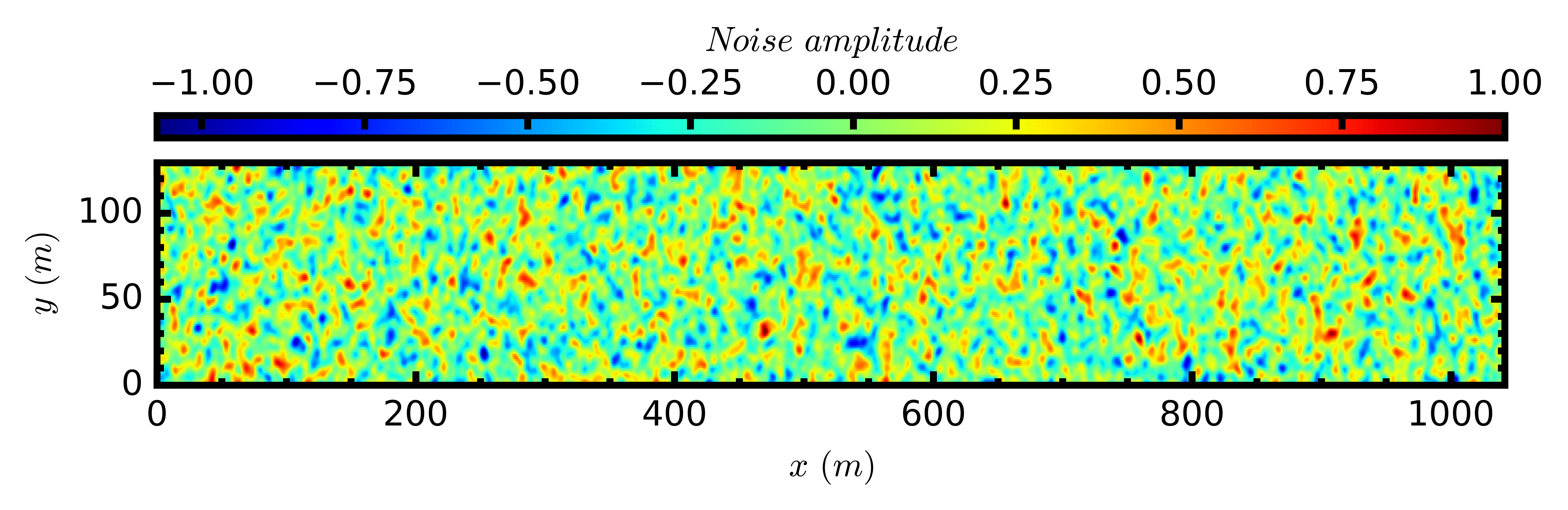
Noise generation
To account for irregularities of the sea bottom we introduce variability on top of the mortality profile. We add a noise with a typical spatial scale to . This noise is generated using the following expression:
| (19) |
where is the inverse Fourier transform, is the modulus of the wavevector of each Fourier component, and is random number between 0 and 1 with a flat probability distribution. The parameter controls the typical spatial scale of noise. The Gaussian shape in Fourier space inhibits long wavelength contributions, in such a way the noise is reasonably smooth. In our simulations we take . Fig. S7 shows the spatial variability of the noise that is added to the mortality profile with a certain amplitude.
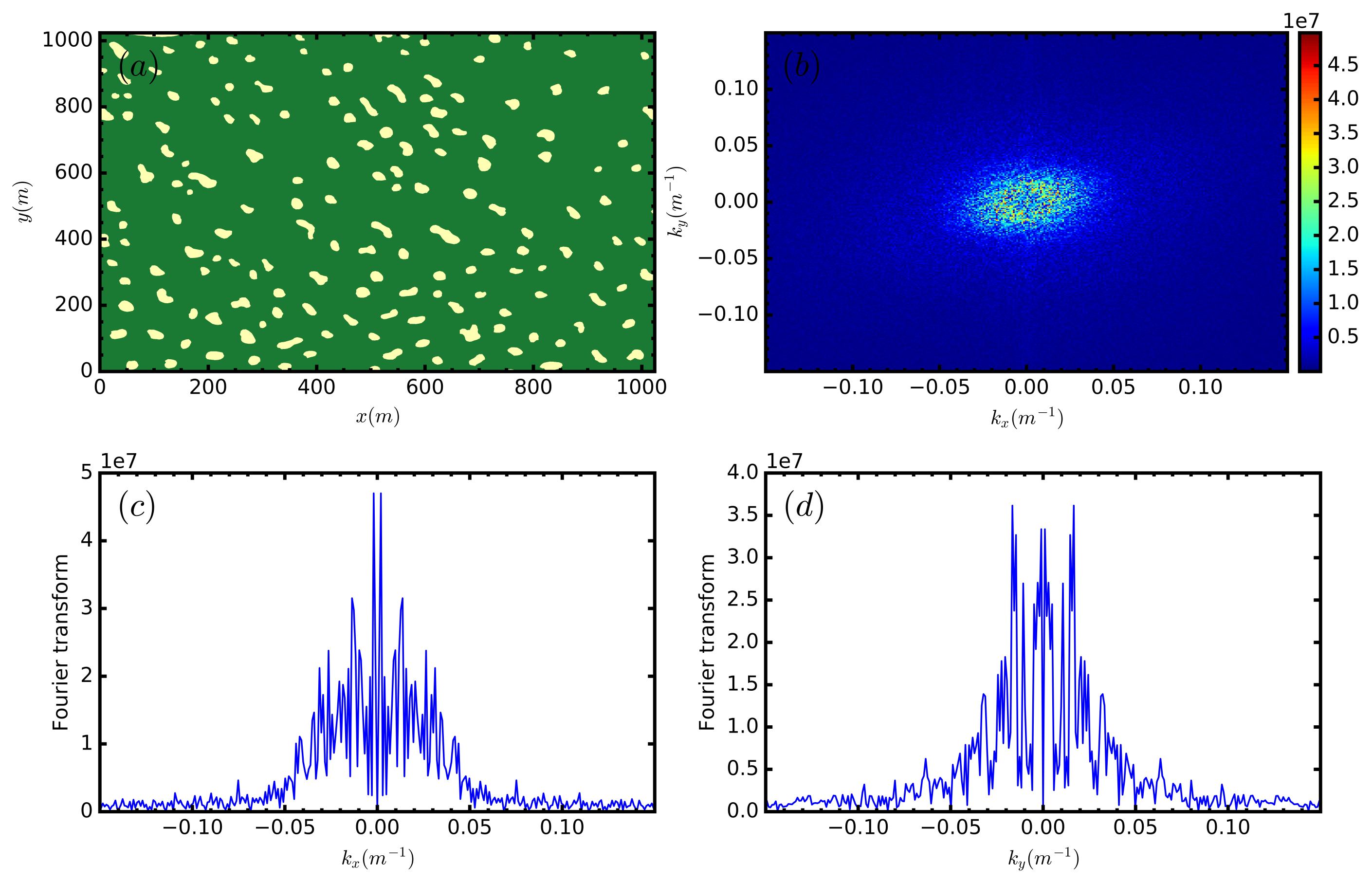
Determination of the characteristic length scale of real
patterns in P. oceanica meadows
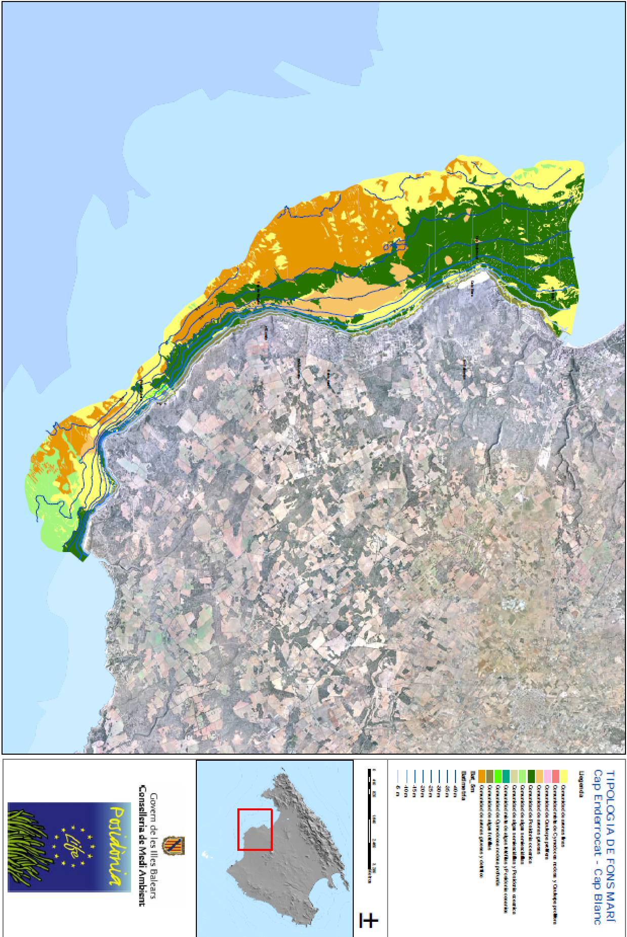
The LIFE Posidonia project realized a mapping of the Posidonia meadows as well as other species such as C. nodosa by using side-scan sonar. As a result, high-resolution images determining the presence/absence of plants are available. These maps, available in low resolution in (http://lifeposidonia.caib.es) show the spatial distribution of the P. oceanica and C. nodosa meadows displaying patterns. Although there are many irregularities, bare holes have a typical size and are separated a characteristic distance. In order to determine the predominant scale of the pattern we analyze the Fourier transform of different regions. In some of them it is difficult to identify a typical length scale. However, a peak indicating a typical length scale is often clearly visible in the Fourier transform. Tables 1 and 2 report the 11 cases that we have used to compute the average wavelength of the patterns. The coordinates of two vertexes of the selected rectangular regions are given in table 1, and the wavenumber of the peak in the Fourier transform is given in table 2. Fig. S11 shows an example of the Fourier transform of a cartography image corresponding to the first row of table 1. The average wavenumber is corresponding to a typical wavelength of 63 .

| 39∘52’58.5”N | 3∘07’43.2”E | 39∘52’25.2”N | 3∘08’26.2”E |
| 39∘53’31.8”N | 3∘05’33.9”E | 39∘52’58.6”N | 3∘06’16.9”E |
| 39∘53’31.8”N | 3∘06’17.0”E | 39∘52’58.5”N | 3∘07’00.1”E |
| 39∘49’55.6”N | 3∘09’52.1”E | 39∘49’22.4”N | 3∘10’35.1”E |
| 39∘48’49.2”N | 3∘10’13.4”E | 39∘48’15.9”N | 3∘10’56.4”E |
| 39∘47’09.6”N | 3∘09’08.6”E | 39∘46’36.4”N | 3∘09’51.6”E |
| 39∘47’09.6”N | 3∘09’51.7”E | 39∘46’36.3”N | 3∘10’34.6”E |
| 39∘47’11.0”N | 3∘10’34.7”E | 39∘46’36.2”N | 3∘11’17.7”E |
| 39∘45’46.4”N | 3∘11’39.1”E | 39∘45’13.1”N | 3∘12’22.0”E |
| 39∘45’29.7”N | 3∘12’22.1”E | 39∘44’56.4”N | 3∘13’05.0”E |
| 39∘45’46.3”N | 3∘12’22.1”E | 39∘45’13.0”N | 3∘13’05.0”E |
| Wave number () |
|---|
| 0.017 |
| 0.018 |
| 0.015 |
| 0.016 |
| 0.015 |
| 0.020 |
| 0.019 |
| 0.019 |
| 0.011 |
| 0.01 |
| 0.015 |
Movie S1
Formation of negative hexagons. Movie showing the formation of a pattern of negative hexagons or fairy circles starting from a noisy populated solution as initial condition. The parameters are the same than in Fig. 2 with . The fast evolution of the system at the beginning is slowed down, as the time indicates, in order to perceive the changes in the pattern as it forms.
Movie S2
Formation of stripes. Movie showing the formation of a stripe pattern starting from a pattern of unstable negative hexagons. The parameters are the same as in Fig. 2 with . The fast evolution of the system at the beginning is slowed down, as the time indicates, in order to perceive the changes in the pattern as it forms.
Movie S3
Formation of positive hexagons. Movie showing the formation of positive hexagons starting from a pattern of unstable negative hexagons. The parameters are the same as in Fig. 2 with . The fast evolution of the system at the beginning is slowed down, as the time indicates, in order to perceive the changes in the pattern as it forms.
Movie S4
Temporal evolution of Fig. 4a. Movie showing the time evolution of Fig. 4a starting from a noisy homogeneous initial condition. The evolution of the system, fast at the beginning of the movie, is slowed down in order to perceive the changes in the pattern as it forms.
Movie S5
Temporal evolution of Fig. 4 (e, f, and h). Movie showing the time evolution of Fig. 4(e, f, and h) starting from a noisy homogeneous initial condition. The evolution of the system, fast at the beginning of the movie, is slowed down in order to perceive the changes in the pattern as it forms.
Movie S6
Temporal evolution of Fig. 5a. Movie showing the time evolution of Fig. 5a starting from a noisy homogeneous initial condition. The evolution of the system, fast at the beginning of the movie, is slowed down in order to perceive the changes in the pattern as it forms.