Explaining Dark Matter and Neutrino Mass in the light of TYPE-II Seesaw Model

Abstract

With the motivation of simultaneously explaining dark matter and neutrino masses, mixing angles, we have invoked the Type-II seesaw model extended by an extra $SU(2)$ doublet $\Phi$. Moreover, we have imposed a $\mathbb{Z}_{2}$ parity on $\Phi$ which remains unbroken as the vacuum expectation value of $\Phi$ is zero.  Consequently, the lightest neutral component of $\Phi$ becomes naturally stable and can be a viable dark matter candidate.  On the other hand, light Majorana masses for neutrinos have been generated following usual Type-II seesaw mechanism. Further in this framework, for the first time we have derived the full set of vacuum stability and unitarity conditions, which must be satisfied to obtain a stable vacuum as well as to preserve the unitarity of the model respectively. Thereafter, we have performed extensive phenomenological studies of both dark matter and neutrino sectors considering all possible theoretical and current experimental constraints. Finally, we have also discussed a qualitative collider signatures of dark matter and associated odd particles at the 13 TeV Large Hadron Collider.

I Introduction

The observation of various satellite borne experiments namely WMAP Hinshaw:2012aka and more recently Planck Ade:2015xua , establish firmly the existence of dark matter in the Universe over the ordinary luminous matter. The results of these experiments are indicating that more than 80% matter content of our Universe has been made of an unknown non-luminous matter or dark matter. In terms of cosmological language, the amount of dark matter present at the current epoch is expressed as $\Omega\,h^{2}=0.1199\pm 0.0027$ Ade:2015xua where $\Omega$ is known as the relic density of dark matter and $h$ is the present value of Hubble parameter $H_{0}$ normalised by 100. In spite of this precise measurement, the particle nature of dark matter still remains an enigma. The least we can say about a dark matter candidate is that it is electrically neutral and must have a lifetime greater than the present age of the Universe. Moreover, N-body simulation requires dark matter candidate to be non-relativistic (cold) at the time of its decoupling from the thermal plasma to explain small scale structures of the Universe Frenk:2012ph . Unfortunately, none of the Standard Model (SM) particles can fulfil all these properties and hence there exist various beyond Standard Model (BSM) theories in the literature Jungman:1995df ; Bertone:2004pz ; Hooper:2007qk ; ArkaniHamed:2008qn ; Kusenko:2009up ; Feng:2010gw containing either at least one or more dark matter candidates. Among the different kinds of dark matter candidates, Weakly Interacting Massive Particle (WIMP) Gondolo:1990dk ; Srednicki:1988ce is the most favourite class and so far, neutralino Jungman:1995df in the supersymmetric extension of the SM is the well studied WIMP candidate. There are also a plethora of well motivated non-supersymmetric BSM theories which have dealt with WIMP type dark matter candidate Silveira:1985rk ; Burgess:2000yq ; McDonald:1993ex ; Barbieri:2006dq ; LopezHonorez:2006gr ; Kim:2008pp ; Hambye:2008bq . Since the interaction strength of a WIMP is around week scale hence various experimental groups Akerib:2016vxi ; Amole:2017dex ; Armengaud:2016cvl ; Agnese:2014aze have been trying to detect it directly over the last two decades by measuring the recoil energies of detector nuclei scattered by WIMPs. However, no such event has been found and as a result, dark matter nucleon elastic scattering cross section is getting severely constrained. Currently most stringent bounds on dark matter spin independent scattering cross section have been reported by the XENON 1T collaboration Aprile:2017iyp . Future direct detection experiment like DARWIN Aalbers:2016jon is expecting to detect or ruled out the WIMP hypothesis by exploring the entire experimentally accessible parameter space of a WIMP (just above the neutrino floor).

On the other hand, neutrinos remain massless in the SM as there is no right handed counterpart of each ${\nu_{\alpha}}_{L}$ where $\alpha$ is the generation index. However, the existence of a tiny nonzero mass difference between $\nu_{\mu}$ and $\nu_{\tau}$ has been first confirmed by the atmospheric neutrino data of Super-kamiokande collaboration Fukuda:1998mi from neutrino oscillation. Thereafter, many experimental groups Ahmad:2002jz ; Araki:2004mb ; Abe:2011sj ; Ahn:2012nd have precisely measured the mass squared differences and mixing angles among different generations of neutrinos. In spite of these wonderful experimental achievements, we still have not properly understood the exact method of neutrino mass generation. There exist various mechanisms for generating tiny neutrino masses at tree level (via seesaw mechanisms) Minkowski:1977sc ; Mohapatra:1979ia ; Magg:1980ut ; Ma:1998dx ; Foot:1988aq ; Ma:2002pf ; Mohapatra:1986bd and beyond Zee:1985id ; Ma:2006km ; Gustafsson:2012vj by adding extra bosonic or fermionic degrees of freedom in the particle spectrum of SM. Moreover, the exact flavour structure in the neutrino sector, which is responsible for generating such a mixing pattern, still remains unknown to us. Furthermore, there are other important issues which are yet to be resolved. For example the particle nature of neutrinos (i.e. Dirac or Majorana fermion), mass hierarchy (i.e. Normal or Inverted), determination of octant for the atmospheric mixing angle $\theta_{23}$, CP violation in the leptonic sector (i.e. measurement of Dirac CP phase $\delta$) etc. More recently, T2K collaboration Abe:2017vif has reported their analysis of neutrino and antineutrino oscillations where they have excluded the hypothesis of CP conservation in the leptonic sector (i.e. $\delta=0$ or $\pi$) at 90% C.L. Their preliminary result indicate a range for $\delta$ lies in between third and fourth quadrant. Other neutrino experiments like DUNE Acciarri:2015uup , NO$\nu$A Adamson:2017gxd etc. will address some of these issues in near future.

In the present article we try to cure both of these lacunae of the SM by introducing a Higgs triplet and an extra Higgs doublet to the particle spectrum of SM. Furthermore, we impose a discrete $\mathbb{Z}_{2}$ symmetry in addition to the SM gauge symmetry. Under this $\mathbb{Z}_{2}$ symmetry the triplet field and the SM particles are even while the extra doublet field is odd. This kind of BSM scenario has been studied earlier in Chen:2014lla . To the best of our knowledge in such set up first time we derive the vacuum stability and unitarity constraints and use these constraints in our phenomenological study. This set up can serve our two fold motivations. First of all, as we have demanded that the extra doublet is odd under $\mathbb{Z}_{2}$ symmetry, consequently the lightest particle of neutral component of this doublet can play the role of viable dark matter candidate in this scenario. Secondly, with the small vacuum expectation value (VEV) of Higgs triplet field, required to satisfy the electroweak precision test, we can explain small neutrino masses by the Type-II seesaw mechanism Magg:1980ut ; Cheng:1980qt ; Lazarides:1980nt ; Mohapatra:1980yp ; Dev:2013ff ; Dev:2013hka without introducing heavy right handed neutrinos. In the present work, we have explored both the normal and inverted hierarchies of neutrino mass spectra. At this point, we would like to mention that all the possible current experimental constraints have been taken into account while we investigate the dark matter related issues as well as the generation of neutrino masses and their mixings.

Apart from providing a viable solution to dark matter problem and neutrino mass generation, this scenario contains several non-standard scalars which can be classified into two categories. In one class we have $\mathbb{Z}_{2}$ even scalars originate from the mixing between triplet fields and SM scalar doublet fields while the three different components of the extra scalar doublet can be represented as $\mathbb{Z}_{2}$ odd scalars. Therefore, one has the opportunity to explore these non-standard scalars at the current and future collider experiments. In literature one can find several articles where the search of $\mathbb{Z}_{2}$ even scalars have been explored in context of the Large Hadron Collider (LHC) Chun:2003ej ; Han:2007bk ; Perez:2008ha ; Han:2015hba ; Han:2015sca ; Mitra:2016wpr as well as at the International Linear Collider (ILC) Shen:2015pih ; Cao:2016hvg ; Blunier:2016peh . However, in this work instead of $\mathbb{Z}_{2}$ even scalars, we have performed collider search of dark matter and the associated $\mathbb{Z}_{2}$ odd scalars at the 13 TeV LHC. Among the different final states, we find an optimistic result for $2\ell+E_{T}/\;\>$ signal at the 13 TeV LHC with an integrated luminosity of 3000$fb^{-1}$.

One should note that, relying on the value of triplet VEV, decay modes of different non-standard scalars show distinct behaviour. From the consideration of electroweak precision test the triplet VEV can not be larger than a few GeV Aoki:2012jj ; Patrignani:2016xqp . However, it can vary from $10^{-9}$ GeV to ${\cal O}(1)$ GeV. Within this range the non-standard Higgs bosons decay in several distinct channels. To be more specific, for ${\rm triplet\leavevmode\nobreak\ VEV}<10^{-4}\leavevmode\nobreak\ \rm GeV$, the doubly charged Higgs dominantly decays into two same-sign leptonic final state. The latest same-sign dilepton searches at the LHC have already put strong lower limit on doubly charged Higgs mass ($>$ 770 - 800 GeV) ATLAS:2017iqw . On the other hand for ${\rm triplet\leavevmode\nobreak\ VEV}>10^{-4}\leavevmode\nobreak\ \rm GeV$, only gauge boson final state or cascade decays of singly charged Higgs (if they are kinematically allowed) are possible Perez:2008ha ; Melfo:2011nx ; Aoki:2011pz ; Han:2015hba ; Han:2015sca . The collider search becomes more involved in this region of triplet VEV due to more complicated decay patterns of the doubly charged Higgs. As a result, the lower bound on the mass of the doubly charged Higgs is very relaxed. Therefore, in this region one can find scenarios where the mass of doubly charged Higgs may goes down to about 100 GeV Melfo:2011nx ; Chabab:2016vqn . In this article, for all practical purposes we have considered the triplet VEV greater than $10^{-4}$ GeV. For example, for the generation of neutrino mass we set triplet VEV at $10^{-3}$ GeV. Whereas, for the purpose of dark matter analysis we show our results for two different values of triplet VEV e.g., $10^{-3}$ GeV and 3 GeV respectively. This is in stark contrast to the Ref. Chen:2014lla where the triplet VEV has been considered less than $10^{-4}$ GeV. Further, for collider study we have fixed the value of triplet VEV at 3 GeV and hence the doubly charged Higgs decays into $W^{\pm}W^{\pm}$ with 100% branching ratio.

We organise this article as follows. First we introduce the model with possible interactions and set our conventions in Sec. II. Within this section we have also evaluated the vacuum stability and unitarity conditions in detail. In Sec. III, we discuss the neutrino mass generation via Type-II seesaw mechanism and explain neutrino oscillation data for normal and inverted hierarchies at $3\sigma$ range. The viability of dark matter candidate proposed in this work has been extensively studied in Sec. IV, considering all possible bounds from direct and indirect experiments. In Sec. V, we show the prospects of collider signature of the dark matter candidate of the present model at 13 TeV LHC. Finally in Sec. VI we summarize our results.

II Type-II Seesaw with Inert Doublet

In this section, we discuss the model briefly. In order to produce a viable dark matter candidate, we introduce a $\mathbb{Z}_{2}$ symmetry in the SM gauge symmetry $SU(2)_{\mathbb{L}}\times U(1)_{\mathbb{Y}}$. Moreover, to generate the neutrino masses and also having a stable dark matter candidate, we incorporate a scalar triplet $\Delta$ with hypercharge two and a scalar doublet $\Phi$ with hypercharge one in the SM fields. Further, we demand that the SM particles and the triplet $\Delta$ are even under $\mathbb{Z}_{2}$ parity while the new doublet $\Phi$ is odd under $\mathbb{Z}_{2}$ parity. The field $\Phi$ cannot develop a VEV at the time of electroweak symmetry breaking as this will break the $\mathbb{Z}_{2}$ symmetry spontaneously, which will jeopardize the dark matter stability. With this newly added $\mathbb{Z}_{2}$ symmetry, we discuss different interaction terms involving SM fields, $\Delta$ and $\Phi$. The total Lagrangian which incorporates all possible interactions can be written as:

$${\cal L}={\cal L}_{\rm Yukawa}+{\cal L}_{\rm Kinetic}-V(H,\Delta,\Phi),$$ (1)

where the relevant kinetic and Yukawa interaction terms are respectively

$${\cal L}_{\rm kinetic} = \left(D_{\mu}H\right)^{\dagger}\left(D^{\mu}H\right)+{\rm Tr}\left[\left(D_{\mu}\Delta\right)^{\dagger}\left(D^{\mu}\Delta\right)\right]+\left(D_{\mu}\Phi\right)^{\dagger}\left(D^{\mu}\Phi\right),$$ (2)

$${\cal L}_{\rm Yukawa} = {\cal L}_{\rm Yukawa}^{\rm SM}-\dfrac{Y^{\nu}_{ij}}{2}L_{i}^{\sf T}\mathcal{C}i\sigma_{2}\Delta L_{j}+{\rm h.c.}\,.$$ (3)

The first two terms of ${\cal L}_{\rm kinetic}$ generate the masses of gauge bosons $W^{\pm}$ and $Z$ by electroweak symmetry breaking mechanism (EWSB), however the third term does not contribute to gauge boson masses as $\Phi$ does not possess any VEV. Here $L_{i}$ represents $SU(2)_{\mathbb{L}}$ doublet of left handed leptons where $i$ being the generational index, $Y^{\nu}$ represents Yukawa coupling and $\mathcal{C}$ is the charge conjugation operator. Further, ${\cal L}_{\rm Yukawa}^{\rm SM}$ denotes the Yukawa interactions for all SM fermions. Later, we will discuss the second term of Yukawa interactions in detail in the neutrino section (Section III). There is no term which involves the coupling between $\Phi$ and the SM fermions as $\Phi$ is odd under $\mathbb{Z}_{2}$ parity while the SM fermions are even under $\mathbb{Z}_{2}$ symmetry. Representations for the doublets $H$ and $\Phi$ are chosen as $H^{\sf T}\equiv(h^{+}\leavevmode\nobreak\ \leavevmode\nobreak\ (v_{d}+\eta^{0}+iz_{1})/\sqrt{2})$ and $\Phi^{\sf T}\equiv(\phi^{+}\leavevmode\nobreak\ \leavevmode\nobreak\ (\phi^{0}+ia^{0})/\sqrt{2})$ respectively. The triplet field $\Delta^{\sf T}(\equiv(\Delta^{1}\leavevmode\nobreak\ \leavevmode\nobreak\ \Delta^{2}\leavevmode\nobreak\ \leavevmode\nobreak\ \Delta^{3}))$ transforms as $({\mathbf{3}},\,2)$ under the $SU(2)_{\mathbb{L}}\times U(1)_{\mathbb{Y}}$ gauge group, so one can write $\Delta=\frac{\sigma^{i}}{\sqrt{2}}\Delta^{i}\,\,(i=1,\,2,\,3)$, which gives a $2\times 2$ representation given in the following:

$$\Delta=\left(\begin{array}[]{cc}\delta^{+}/\sqrt{2}&\delta^{++}\\ \delta^{0}&-\delta^{+}/\sqrt{2}\\ \end{array}\right)\,.\$$ (6)

In the above $\Delta^{1}=(\delta^{++}+\delta^{0})/\sqrt{2},\leavevmode\nobreak\ \Delta^{2}=i(\delta^{++}-\delta^{0})/\sqrt{2},\leavevmode\nobreak\ \Delta^{3}=\delta^{+}$. The neutral component of the triplet field can be expressed as $\delta^{0}=(v_{t}+\xi^{0}+iz_{2})/\sqrt{2}$ where $v_{d}$ and $v_{t}$ are vacuum expectation values of the doublet $H$ and triplet $\Delta$ respectively. The covariant derivative of the scalar field $\Delta$ is given by,

$$D_{\mu}\Delta=\partial_{\mu}\Delta+i\frac{g_{2}}{2}[\sigma^{a}W_{\mu}^{a},\Delta]+ig_{1}B_{\mu}\Delta\qquad(a=1,\,2,\,3)\,.$$ (7)

Here $\sigma^{i}$’s are the Pauli matrices while $g_{2}$ and $g_{1}$ are coupling constants for the gauge groups $SU(2)_{\mathbb{L}}$ and $U(1)_{\mathbb{Y}}$ respectively.

Let us discuss the scalar potential given in the following Chen:2014lla :

$$V(H,\Delta,\Phi) = -m^{2}_{H}(H^{\dagger}H)+\frac{\lambda}{4}(H^{\dagger}H)^{2}+M^{2}_{\Delta}{\rm Tr}(\Delta^{\dagger}\Delta)+\left(\mu H^{\sf T}i\sigma_{2}\Delta^{\dagger}H+{\rm h.c.}\right)\,$$ (8)

$$+\lambda_{1}(H^{\dagger}H){\rm Tr}(\Delta^{\dagger}\Delta)+\lambda_{2}\left[{\rm Tr}(\Delta^{\dagger}\Delta)\right]^{2}+\lambda_{3}{\rm Tr}(\Delta^{\dagger}\Delta)^{2}+\lambda_{4}(H^{\dagger}\Delta\Delta^{\dagger}H)\,$$

$$+m^{2}_{\Phi}(\Phi^{\dagger}\Phi)+\lambda_{\Phi}(\Phi^{\dagger}\Phi)^{2}+\lambda_{5}(H^{\dagger}H)(\Phi^{\dagger}\Phi)+\lambda_{6}(H^{\dagger}\Phi\Phi^{\dagger}H)\,$$

$$+\lambda_{7}(\Phi^{\dagger}\Phi){\rm Tr}(\Delta^{\dagger}\Delta)+\lambda_{8}(\Phi^{\dagger}\Delta\Delta^{\dagger}\Phi)+\lambda_{9}\left[(\Phi^{\dagger}H)^{2}+{\rm h.c.}\right]\,$$

$$+\left(\tilde{\mu}\Phi^{\sf T}i\sigma_{2}\Delta^{\dagger}\Phi+{\rm h.c.}\right).$$

Here, $\lambda$, $\lambda_{\Phi}$ and $\lambda_{i}$ ($i=1,\ldots 9$) are dimensionless coupling constants, while $m_{H}$, $m_{\Phi}$, $M_{\Delta}$, $\mu$ and $\tilde{\mu}$ are mass parameters of the above potential. Whereas $\lambda_{9}$, $\mu$ and $\tilde{\mu}$ are the only terms which can generate CP phases, as the other terms of the potential are self-conjugate. However, two of them can be removed by redefining the fields $H$, $\Phi$ and $\Delta$. Furthermore, we assume that $m^{2}_{H}>0$ for the spontaneous breaking of above mentioned gauge group.

After EWSB we obtain a doubly charged scalar $H^{\pm\pm}$ including a singly charged scalar, $H^{\pm}$, a pair of neutral CP even Higgs ($h^{0},H^{0}$), a CP odd scalar ($A^{0}$) and as usual three massless Goldstone bosons ($G^{\pm},G^{0}$). Further, we also have three particles ($\phi^{\pm}$, $\phi^{0}$, and $a^{0}$) which are members of the inert $SU(2)$ doublet. The mass eigenvalues for the $\mathbb{Z}_{2}$ even physical scalar are given by Arhrib:2011uy :

$$M^{2}_{H^{\pm\pm}} = \frac{\sqrt{2}\mu v^{2}_{d}-\lambda_{4}v^{2}_{d}v_{t}-2\lambda_{3}v^{3}_{t}}{2v_{t}},$$ (9)

$$M^{2}_{H^{\pm}} = \frac{(v_{d}^{2}+2v^{2}_{t})(2\sqrt{2}\mu-\lambda_{4}v_{t})}{4v_{t}},$$ (10)

$$M^{2}_{A^{0}} = \frac{\mu(v_{d}^{2}+4v^{2}_{t})}{\sqrt{2}v_{t}},$$ (11)

$$M^{2}_{h^{0}} = \frac{1}{2}\left(A+C-\sqrt{(A-C)^{2}+4B^{2}}\right),$$ (12)

$$M^{2}_{H^{0}} = \frac{1}{2}\left(A+C+\sqrt{(A-C)^{2}+4B^{2}}\right),$$ (13)

with

$$A = \frac{\lambda}{2}v_{d}^{2},$$ (14)

$$B = v_{d}[-\sqrt{2}\mu+(\lambda_{1}+\lambda_{4})v_{t}],$$ (15)

$$C = \frac{\sqrt{2}\mu v^{2}_{d}+4(\lambda_{2}+\lambda_{3})v^{3}_{t}}{2v_{t}},$$ (16)

while the mass eigenvalues of $\mathbb{Z}_{2}$ odd scalars are:

$$M^{2}_{\phi^{0}} = m^{2}_{\Phi}+\frac{1}{2}(\lambda_{5}+\lambda_{6})v^{2}_{d}+\frac{1}{2}(\lambda_{7}+\lambda_{8})v^{2}_{t}+\lambda_{9}v^{2}_{d}-\sqrt{2}\tilde{\mu}v_{t},$$ (17)

$$M^{2}_{a^{0}} = m^{2}_{\Phi}+\frac{1}{2}(\lambda_{5}+\lambda_{6})v^{2}_{d}+\frac{1}{2}(\lambda_{7}+\lambda_{8})v^{2}_{t}-\lambda_{9}v^{2}_{d}+\sqrt{2}\tilde{\mu}v_{t},$$ (18)

$$M^{2}_{\phi^{\pm}} = m^{2}_{\Phi}+\frac{1}{2}\lambda_{5}v^{2}_{d}+\frac{1}{2}\lambda_{7}v^{2}_{t}.$$ (19)

The mixing between the SM doublet and the triplet scalar fields in the charged, CP even as well as CP odd scalar sectors are respectively given by:

$$\left(\begin{array}[]{c}G^{\pm}\\ H^{\pm}\end{array}\right) = \left(\begin{array}[]{cc}\cos\beta^{\prime}&\sin\beta^{\prime}\\ -\sin\beta^{\prime}&\cos\beta^{\prime}\end{array}\right)\left(\begin{array}[]{c}h^{\pm}\\ \delta^{\pm}\end{array}\right),$$ (26)

$$\left(\begin{array}[]{c}h^{0}\\ H^{0}\end{array}\right) = \left(\begin{array}[]{cc}\cos\alpha&\sin\alpha\\ -\sin\alpha&\cos\alpha\end{array}\right)\left(\begin{array}[]{c}\eta^{0}\\ \xi^{0}\end{array}\right),$$ (33)

$$\left(\begin{array}[]{c}G^{0}\\ A^{0}\end{array}\right) = \left(\begin{array}[]{cc}\cos\beta&\sin\beta\\ -\sin\beta&\cos\beta\end{array}\right)\left(\begin{array}[]{c}z_{1}\\ z_{2}\end{array}\right),$$ (40)

and the respective mixing angles are given by:

$$\tan\beta^{\prime} = \frac{\sqrt{2}\,v_{t}}{v_{d}},$$ (41)

$$\tan\beta = \frac{2\,v_{t}}{v_{d}}=\sqrt{2}\tan\beta^{\prime},$$ (42)

$$\tan{2\alpha} = \frac{2B}{A-C}\,,$$ (43)

where the expressions of $A$, $B$ and $C$ are already given in Eq. 13.

II.1 Different constraints

Before going to study the phenomenological aspects of neutrino and dark matter sectors, it is necessary to check various constraints from theoretical considerations like vacuum stability, unitarity of the scattering matrices and perturbativity. Further, the model parameters also need to satisfy the phenomenological constraints arising from electroweak precision test and Higgs signal strength. Therefore, to serve the purposes we need to choose a set of free parameters of this model. In practice, a convenient set of free parameters are given in the following, however some of them are not independent:

$$\{\tan{\alpha},M_{H^{\pm\pm}},M_{H^{\pm}},M_{H^{0}}(=M_{A^{0}}),M_{\phi^{0}},M_{\phi^{\pm}},\lambda_{\Phi},\lambda_{5},\lambda_{6},\lambda_{7},\lambda_{8},\lambda_{9}\}\,.$$ (44)

II.1.1 Vacuum stability bounds:

This section has been dedicated to derive the necessary and sufficient conditions for the stability of the vacuum. These conditions come from requiring that the potential given in Eq. 8 be bounded from below when the scalar fields become large in any direction of the field space. The constraints ensuring boundedness from below (BFB) of the present potential have not been studied in the literature so far. It would thus be very relevant to derive these constraints in the present model. For large field values, the potential given in Eq. 8 is generically dominated by the quartic part of the potential. Hence, in this limit we can ignore any terms with dimensionful couplings, mass terms or soft terms. So the general potential given in Eq. 8 can be written as in the following way which contains only the quartic terms,

$$V^{(4)}(H,\Delta,\Phi) = \frac{\lambda}{4}(H^{\dagger}H)^{2}+\lambda_{1}(H^{\dagger}H){\rm Tr}(\Delta^{\dagger}\Delta)+\lambda_{2}\left[{\rm Tr}(\Delta^{\dagger}\Delta)\right]^{2}+\lambda_{3}{\rm Tr}(\Delta^{\dagger}\Delta)^{2}$$ (45)

$$+\lambda_{4}(H^{\dagger}\Delta\Delta^{\dagger}H)\,+\lambda_{\Phi}(\Phi^{\dagger}\Phi)^{2}+\lambda_{5}(H^{\dagger}H)(\Phi^{\dagger}\Phi)+\lambda_{6}(H^{\dagger}\Phi\Phi^{\dagger}H)\,$$

$$+\lambda_{7}(\Phi^{\dagger}\Phi){\rm Tr}(\Delta^{\dagger}\Delta)+\lambda_{8}(\Phi^{\dagger}\Delta\Delta^{\dagger}\Phi)+\lambda_{9}\left[(\Phi^{\dagger}H)^{2}+{\rm h.c.}\right].$$

To determine the BFB conditions we have used copositivity criteria as given in Ref. Kannike:2012pe . For this purpose we need to express the scalar potential $V^{(4)}$ in a biquadratic form $A_{ij}\psi^{2}_{i}\psi^{2}_{j}$, where $\psi_{i}\equiv H,\Delta,\Phi$. If the matrix $A_{ij}$ is copositive then we can demand that the potential is bounded from below. Let us write down the matrix in our case:

$$A=\left(\begin{array}[]{ccc}\frac{1}{4}{\lambda}&\frac{1}{2}{(\lambda_{1}+\xi\lambda_{4})}&\frac{1}{2}{[\lambda_{5}+\rho^{2}(\lambda_{6}-2|\lambda_{9}|)]}\\ \frac{1}{2}{(\lambda_{1}+\xi\lambda_{4})}&(\lambda_{2}+\zeta\lambda_{3})&\frac{1}{2}{(\lambda_{7}+\xi^{\prime}\lambda_{8})}\\ \frac{1}{2}{[\lambda_{5}+\rho^{2}(\lambda_{6}-2|\lambda_{9}|)]}&\frac{1}{2}{(\lambda_{7}+\xi^{\prime}\lambda_{8})}&\lambda_{\Phi}\end{array}\right)\,.$$ (46)

The parameters $\xi$, $\xi^{\prime}$, $\zeta$ and $\rho$ appearing in the matrix elements are required to determine all the necessary and sufficient BFB conditions. The detail illustrations of the parameters can be found in Arhrib:2011uy where two fields (one doublet and a triplet) have been considered. However, in our case we have three different fields (two doublets and a triplet). Using the prescription given in Ref. Arhrib:2011uy , we have defined the parameters in the following way,

$$\zeta\equiv{\rm Tr}(\Delta^{\dagger}{\Delta})^{2}/[{\rm Tr}(\Delta^{\dagger}{\Delta})]^{2},$$ (47)

$$\rho\equiv|H^{\dagger}\Phi|/|H||\Phi|,$$ (48)

$$\xi\equiv(H^{\dagger}\Delta\Delta^{\dagger}H)/(H^{\dagger}{H}\leavevmode\nobreak\ {\rm Tr}(\Delta^{\dagger}{\Delta})),$$ (49)

$$\xi^{\prime}\equiv(\Phi^{\dagger}\Delta\Delta^{\dagger}\Phi)/(\Phi^{\dagger}{\Phi}\leavevmode\nobreak\ {\rm Tr}(\Delta^{\dagger}{\Delta})).$$ (50)

The $upper$ and $lower$ limits of these parameters are given as [$\frac{1}{2},1$], [$0,1$], [$0,1$] and [$0,1$] respectively Arhrib:2011uy . To determine the all possible BFB conditions of the scalar potential, we consider both the limits of these parameters and respect the copositivity criteria. Finally, we can write down the following BFB conditions by demanding the symmetric matrix $A_{ij}$ is copositive Kannike:2012pe .

$$\lambda\geq 0,$$ (51)

$$(\lambda_{2}+\zeta\lambda_{3})\geq 0,$$ (52)

$$\lambda_{\Phi}\geq 0,$$ (53)

$${(\lambda_{1}+\xi\lambda_{4})}+\sqrt{\lambda(\lambda_{2}+\zeta\lambda_{3})}\geq 0,$$ (54)

$${\lambda_{5}+\rho^{2}(\lambda_{6}-2|\lambda_{9}|)}+\sqrt{\lambda\lambda_{\Phi}}\geq 0,$$ (55)

$${(\lambda_{7}+\xi^{\prime}\lambda_{8})}+2\sqrt{(\lambda_{2}+\zeta\lambda_{3})\lambda_{\Phi}}\geq 0,$$ (56)

$$\sqrt{\lambda(\lambda_{2}+\zeta\lambda_{3})\lambda_{\Phi}}+(\lambda_{1}+\xi\lambda_{4})\sqrt{\lambda_{\Phi}}+[\lambda_{5}+\rho^{2}(\lambda_{6}-2|\lambda_{9}|)]\sqrt{\lambda_{2}+\zeta\lambda_{3}}+\frac{(\lambda_{7}+\xi^{\prime}\lambda_{8})}{2}\sqrt{\lambda}$$ (57)

$$+{\tiny\sqrt{\left\{(\lambda_{1}+\xi\lambda_{4})+\sqrt{\lambda(\lambda_{2}+\zeta\lambda_{3})}\right\}\left\{(\lambda_{7}+\xi^{\prime}\lambda_{8})+2\sqrt{\lambda_{\Phi}(\lambda_{2}+\zeta\lambda_{3})}\right\}\left\{[\lambda_{5}+\rho^{2}(\lambda_{6}-2|\lambda_{9}|)]+\sqrt{\lambda\lambda_{\Phi}}\right\}}\geq 0}.$$

Substituting the lower and upper limits of the parameters, one can get the full set of vacuum stability conditions given in Appendix B (see Eq. B-3 to Eq. B-10h).

II.1.2 Unitarity bounds:

In this section we discuss the unitarity constraints on the parameters of scalar potential by using the tree-level unitarity of various scattering processes. One can find the scalar-scalar scattering, gauge boson-gauge boson scattering and scalar-gauge boson scattering in the context of SM in Appelquist:1971yj ; Cornwall:1974km ; Lee:1977eg . In the case of various extended Higgs sector scenario, the generalizations of such constraints can be found in literature Kanemura:1993hm ; Akeroyd:2000wc ; Aoki:2007ah ; Gogoladze:2008ak . It has been a well known fact that in the high energy limit using equivalence theorem Lee:1977eg ; Cornwall:1973tb ; Chanowitz:1985hj one can replace longitudinal gauge bosons by those of the corresponding Nambu-Goldstone bosons in $2\rightarrow 2$ scattering. Hence, following this prescription in the current model, our main focus is to consider only the Higgs-Goldstone interactions of the scalar potential given in Eq. 8. Furthermore, under this situation the $2$-body scalar scattering processes are dominated by the quartic interactions only.

To determine the unitarity constraints, it has been a usual trend to calculate the $\mathcal{S}$-matrix amplitude in the basis of unrotated states, corresponding to the fields before electroweak symmetry breaking. Because, in this situation the quartic scalar vertices have a much simpler form with respect to the complicated functions of $\lambda_{i}$, $\lambda_{\Phi}$, $\alpha$ and $\beta$ involved in the physical basis ($H^{\pm\pm}$, $H^{\pm}$, $G^{\pm}$, $h^{0}$, $H^{0}$, $A^{0}$, $G^{0}$, $\phi^{0}$, $\phi^{\pm}$ and $a^{0}$). So in the unrotated basis ($\delta^{\pm\pm}$, $\delta^{\pm}$, $h^{\pm}$, $\phi^{\pm}$, $\eta^{0}$, $\xi^{0}$, $z_{1}$, $z_{2}$, $\phi^{0}$ and $a^{0}$), we study full set of $2$-body scalar scattering processes which lead to a $68\times 68$ $\mathcal{S}$-matrix. This matrix can be decomposed into 7 block submatrices with definite charge. For example, $\mathcal{M}_{1}(18\times 18)$, $\mathcal{M}_{2}(10\times 10)$ and $\mathcal{M}_{3}(3\times 3)$ corresponding to neutral charged states, $\mathcal{M}_{4}(21\times 21)$ corresponding to the singly charged states, $\mathcal{M}_{5}(12\times 12)$ corresponding to the doubly charged states, $\mathcal{M}_{6}(3\times 3)$ corresponding to the triply charged states and finally $\mathcal{M}_{7}(1\times 1)$ corresponding to the unique quartic charged state. These submatrices are hermitian, so the eigenvalues will always be real-valued.

To this end, we would like to mention that in the following cases we will determine the eigenvalues of the above mentioned submatrices. However, there is a caveat. The structure of some of the submatrices are very challenging, so it is not possible to find out the analytic form of all the eigenvalues of those matrices. However, using numerical technique given in Adhikary:2013bma we can derive the remaining eigenvalues. Eventually, we will have all the full set of eigenvalues by which we will put the unitarity constraints on the model parameters.

The first submatrix ${\mathcal{M}}_{1}$ corresponds to the scatterings whose initial and final states are one of the following:

$$\bigg{\{}h^{+}\delta^{-},\delta^{+}h^{-},\phi^{+}\delta^{-},\delta^{+}\phi^{-},h^{+}\phi^{-},\phi^{+}h^{-},\eta^{0}z_{2},\xi^{0}z_{1},z_{1}z_{2},\eta^{0}\xi^{0},\phi^{0}\eta^{0},\phi^{0}z_{1},\eta^{0}a^{0},a^{0}z_{1},\phi^{0}\xi^{0},\phi^{0}z_{2},$$

$$a^{0}\xi^{0},a^{0}z_{2}\bigg{\}},$$

Eigenvalues of ${\mathcal{M}}_{1}$ are:

$$\bigg{\{}\lambda_{1},\lambda_{1},\lambda_{1}+\lambda_{4},\lambda_{1}+\lambda_{4},\lambda_{1}+\frac{3\lambda_{4}}{2},\lambda_{1}+\frac{3\lambda_{4}}{2},\lambda_{5}+\lambda_{6},\lambda_{5}+\lambda_{6},\lambda_{7},\lambda_{7},\lambda_{7}+\lambda_{8},$$

$$\lambda_{7}+\lambda_{8},\lambda_{7}+\frac{3\lambda_{8}}{2},\lambda_{7}+\frac{3\lambda_{8}}{2},\lambda_{5}+2\lambda_{6}-6\lambda_{9},\lambda_{5}-2\lambda_{9},\lambda_{5}+2\lambda_{9},\lambda_{5}+2\lambda_{6}+6\lambda_{9}\bigg{\}}.$$

The second submatrix ${\mathcal{M}}_{2}$ corresponds to the scatterings whose initial and final states are one of the following:

$$\bigg{\{}h^{+}h^{-},\delta^{+}\delta^{-},\frac{z_{1}z_{1}}{\sqrt{2}},\frac{z_{2}z_{2}}{\sqrt{2}},\frac{\eta^{0}\eta^{0}}{\sqrt{2}},\frac{\xi^{0}\xi^{0}}{\sqrt{2}},\phi^{+}\phi^{-},\frac{\phi^{0}\phi^{0}}{\sqrt{2}},\frac{a^{0}a^{0}}{\sqrt{2}},\delta^{++}\delta^{--}\bigg{\}},$$

Eigenvalues of ${\mathcal{M}}_{2}$ are:

$$\bigg{\{}2\lambda_{2},2(\lambda_{2}+\lambda_{3}),\frac{1}{4}\left(\lambda-\sqrt{64\lambda^{2}_{9}+(\lambda-4\lambda_{\Phi})^{2}}+4\lambda_{\Phi}\right),\frac{1}{4}\left(\lambda+\sqrt{64\lambda^{2}_{9}+(\lambda-4\lambda_{\Phi})^{2}}+4\lambda_{\Phi}\right)\bigg{\}}.$$

Rest of the six eigenvalues have been obtained by numerically solving the cubic Eqs. A-1 and A-2 given in Appendix A.

The third submatrix ${\mathcal{M}}_{3}$ corresponds to the scatterings whose initial and final states are one of the following:

$$\bigg{\{}\eta^{0}z_{1},\xi^{0}z_{2},\phi^{0}a^{0}\bigg{\}},$$

Eigenvalues of ${\mathcal{M}}_{3}$ are:

$$\bigg{\{}2(\lambda_{2}+\lambda_{3}),\frac{1}{4}\left(\lambda-\sqrt{64\lambda^{2}_{9}+(\lambda-4\lambda_{\Phi})^{2}}+4\lambda_{\Phi}\right),\frac{1}{4}\left(\lambda+\sqrt{64\lambda^{2}_{9}+(\lambda-4\lambda_{\Phi})^{2}}+4\lambda_{\Phi}\right)\bigg{\}}.$$

The fourth submatrix ${\mathcal{M}}_{4}$ corresponds to the scatterings, where one charge channels occur for $2\rightarrow 2$ scattering between the 20 charged states:

$$\bigg{\{}\eta^{0}h^{+},\xi^{0}h^{+},z_{1}h^{+},z_{2}h^{+},h\delta^{+},\xi^{0}\delta^{+},z_{1}\delta^{+},z_{2}\delta^{+},\eta^{0}\phi^{0},\xi^{0}\phi^{+},z_{1}\phi^{+}z_{2}\phi^{+},h^{+}\phi^{0},h^{+}a^{0},\delta^{+}\phi^{0},\delta^{+}a^{0},$$

$$\phi^{+}\phi^{0},\phi^{+}a^{0},\delta^{++}\delta^{-},\delta^{++}h^{-},\delta^{++}\phi^{-}\bigg{\}},$$

Eigenvalues of ${\mathcal{M}}_{4}$ are:

$$\bigg{\{}\text{$\lambda_{1}$},\text{$\lambda_{1}$},2\text{$\lambda_{2}$},2(\text{$\lambda_{2}$}+\text{$\lambda_{3}$}),\text{$\lambda_{1}$}-\frac{\text{$\lambda_{4}$}}{2},\text{$\lambda_{1}$}+\text{$\lambda_{4}$},\text{$\lambda_{1}$}+\frac{3\text{$\lambda_{4}$}}{2},\text{$\lambda_{5}$}-\text{$\lambda_{6}$},\text{$\lambda_{5}$}+\text{$\lambda_{6}$},\text{$\lambda_{7}$},\text{$\lambda_{7}$},\text{$\lambda_{7}$}-\frac{\text{$\lambda_{8}$}}{2},$$

$$\text{$\lambda_{7}$}+\text{$\lambda_{8}$},\text{$\lambda_{7}$}+\frac{3\text{$\lambda_{8}$}}{2},\text{$\lambda_{5}$}-2\text{$\lambda_{9}$},\text{$\lambda_{5}$}+2\text{$\lambda_{9}$},\frac{1}{4}\left(\lambda+\sqrt{64\text{$\lambda^{2}_{9}$}+(\lambda-4\lambda_{\Phi})^{2}}+4\lambda_{\Phi}\right),$$

$$\frac{1}{4}\left(\lambda-\sqrt{64\text{$\lambda^{2}_{9}$}+(\lambda-4\lambda_{\Phi})^{2}}+4\lambda_{\Phi}\right)\bigg{\}}.$$

Remaining three eigenvalues have been obtained from the cubic Eq. A-2 (see Appendix A) using numerical technique.

The fifth submatrix ${\mathcal{M}}_{5}$ corresponds to the scatterings, where double charge channels occur for $2\rightarrow 2$ scattering between the 12 charged states:

$$\bigg{\{}\frac{h^{+}h^{+}}{\sqrt{2}},\frac{\delta^{+}\delta^{+}}{\sqrt{2}},\delta^{+}h^{+},\frac{\phi^{+}\phi^{+}}{\sqrt{2}},\phi^{+}\delta^{+},\phi^{+}h^{+},\delta^{++}\xi^{0},\delta^{++}z_{2},\delta^{++}z_{1},\delta^{++}\eta^{0},\delta^{++}\phi^{0},\delta^{++}a^{0}\bigg{\}},$$

Eigenvalues of ${\mathcal{M}}_{5}$ are:

$$\bigg{\{}\text{$\lambda_{1}$},2\text{$\lambda_{2}$},2\text{$\lambda_{2}$}-\text{$\lambda_{3}$},2(\text{$\lambda_{2}$}+\text{$\lambda_{3}$}),\text{$\lambda_{1}$}-\frac{\text{$\lambda_{4}$}}{2},\text{$\lambda_{1}$}+\text{$\lambda_{4}$},\text{$\lambda_{5}$}+\text{$\lambda_{6}$},\text{$\lambda_{7}$},\text{$\lambda_{7}$}-\frac{\text{$\lambda_{8}$}}{2},\text{$\lambda_{7}$}+\text{$\lambda_{8}$},$$

$$\frac{1}{4}\left(\lambda+\sqrt{64\text{$\lambda^{2}_{9}$}+(\lambda-4\lambda_{\Phi})^{2}}+4\lambda_{\Phi}\right),\frac{1}{4}\left(\lambda-\sqrt{64\text{$\lambda^{2}_{9}$}+(\lambda-4\lambda_{\Phi})^{2}}+4\lambda_{\Phi}\right)\bigg{\}}.$$

The sixth submatrix ${\mathcal{M}}_{6}$ corresponds to the scatterings, where triple charge channels occur for $2\rightarrow 2$ scattering between the 3 charged states:

$$\bigg{\{}\delta^{++}h^{+},\delta^{++}\delta^{+},\delta^{++}\phi^{+}\bigg{\}},$$

Eigenvalues of ${\mathcal{M}}_{6}$ are: {2($\lambda_{2}$+$\lambda_{3}$),  $\lambda_{1}$+$\lambda_{4}$,  $\lambda_{7}$+$\lambda_{8}$}. Finally, there is unique quadruple charged state $\frac{\delta^{++}\delta^{++}}{\sqrt{2}}$ which leads to eigenvalue

$${\mathcal{M}}_{7}=2(\lambda_{2}+\lambda_{3}).$$

These eigenvalues, can be labelled as $a_{i}$, then the $\mathcal{S}$-matrix unitarity constraint for elastic scattering demands $|{\rm Re}(a_{i})|\leq\frac{1}{2}$ Lee:1977eg . Using this condition we generate the following relations. However, these conditions are not the full set of unitarity conditions as we have already mentioned that some of the eigenvalues of few submatrices are evaluated numerically. Hence, using the following conditions,

$$|\lambda_{1}|\leq 8\pi,\,|2\lambda_{2}|\leq 8\pi,\,|\lambda_{1}+\lambda_{4}|\leq 8\pi,\,|2(\lambda_{2}+\lambda_{3})|\leq 8\pi,\,\left|\lambda_{1}+\frac{3\lambda_{4}}{2}\right|\leq 8\pi,\,\left|\lambda_{1}-\frac{\lambda_{4}}{2}\right|\leq 8\pi,$$

$$|2\lambda_{2}-\lambda_{3}|\leq 8\pi,\,|\lambda_{5}+2\lambda_{6}-6\lambda_{9}|\leq 8\pi,\,|\lambda_{5}+2\lambda_{6}+6\lambda_{9}|\leq 8\pi,\,|\lambda_{5}+2\lambda_{9}|\leq 8\pi,\,|\lambda_{5}-2\lambda_{9}|\leq 8\pi,$$

$$|\lambda_{5}-\lambda_{6}|\leq 8\pi,\,|\lambda_{5}+\lambda_{6}|\leq 8\pi,\,|\lambda_{7}|\leq 8\pi,\,|\lambda_{7}+\lambda_{8}|\leq 8\pi,\,\left|\lambda_{7}+\frac{3\lambda_{8}}{2}\right|\leq 8\pi,\,\left|\lambda_{7}-\frac{\lambda_{8}}{2}\right|\leq 8\pi,$$

$$\bigg{|}\frac{1}{4}\left(\lambda+\sqrt{64\text{$\lambda^{2}_{9}$}+(\lambda-4\lambda_{\Phi})^{2}}+4\lambda_{\Phi}\right)\bigg{|}\leq 8\pi,\,\bigg{|}\frac{1}{4}\left(\lambda-\sqrt{64\text{$\lambda^{2}_{9}$}+(\lambda-4\lambda_{\Phi})^{2}}+4\lambda_{\Phi}\right)\bigg{|}\leq 8\pi,$$ (58)

and numerically evaluated six eigenvalues (whose absolute value should be $\leq 8\pi$) we have imposed full set of unitarity constraints on the model parameters.

II.1.3 Perturbativity:

If we demand that the model in the present work behaves as a perturbative quantum field theory at any energy scale, then we have to ensure the following conditions. For the scalar quartic coupling $\lambda,\lambda_{\Phi},\lambda_{i}(i=1-9)$, the perturbativity criterion is,

$$|\lambda|,|\lambda_{\Phi}|,|\lambda_{i}|<4\pi.$$ (59)

The corresponding constraints for the gauge and Yukawa interactions are,

$$g_{i},y_{i}<\sqrt{4\pi},$$ (60)

where, $g_{i}$’s and $y_{i}$’s are the gauge and Yukawa coupling constants respectively.

II.1.4 Constraints from electroweak precision test:

Electroweak precision test (EWPT) can be considered as a very useful tool in constraining any BSM scenario. As the current scenario contains several non-standard scalars, hence they contribute to the electroweak precision observables, the $S,T,U$ parameters Lavoura:1993nq ; Barbieri:2006dq ; Chun:2012jw ; Aoki:2012jj . The stringent bound comes from the $T$-parameter which imposes strict limit on the mass splitting between the non-standard scalars. Therefore, we tune the relative mass splitting between the non-standard scalars in such a way for which the present scenario satisfy the constraints from EWPT Baak:2014ora . Further, the electroweak precision data constraint the $\rho$-parameter to be very close to its SM value of unity and from the latest data Patrignani:2016xqp one gets an upper bound on $v_{t}\mathrel{\mathchoice{\vbox{\offinterlineskip\halign{\hfil$\displaystyle#$\hfil\cr<\cr\sim\cr}}}{\vbox{\offinterlineskip\halign{\hfil$\textstyle#$\hfil\cr<\cr\sim\cr}}}{\vbox{\offinterlineskip\halign{\hfil$\scriptstyle#$\hfil\cr<\cr\sim\cr}}}{\vbox{\offinterlineskip\halign{\hfil$\scriptscriptstyle#$\hfil\cr<\cr\sim\cr}}}}4$ GeV which we maintain in our analysis.

II.1.5 Constraints from Higgs signal strength ($\mu_{\gamma\gamma}=\frac{\sigma(pp\rightarrow h)_{\rm BSM}\times{\rm BR}(h\rightarrow\gamma\gamma)_{\rm BSM}}{\sigma(pp\rightarrow h)_{\rm SM}\times{\rm BR}(h\rightarrow\gamma\gamma)_{\rm SM}}$):

Moreover, apart from the above mentioned theoretical constraints, it is necessary to incorporate the constraints from LHC data in the model. As in the present model all the decay widths and cross sections are modified with respect to that of the SM predictions so in our analysis we have constrained the parameter space of this model by the present LHC Higgs data ATLAS:2016nke .

III Neutrino masses and mixings

In this section, we have tried to explain the origin of neutrino masses and their intergenerational mixing angles. In the present model, as we have one $SU(2)_{\mathbb{L}}$ scalar triplet $\Delta$ (Eq. 6), hence one can generate Majorana mass term for the SM neutrinos using Type-II seesaw mechanism Magg:1980ut ; Ma:1998dx . The Yukawa interaction term which is responsible for the Majorana masses of SM neutrinos is given by

$${\cal L}_{\rm Yukawa}\supset-\dfrac{Y^{\nu}_{ij}}{2}L_{i}^{\sf T}\mathcal{C}\,i\sigma_{2}\,\Delta\,L_{j}+{\rm h.c.}\,$$ (61)

where $Y^{\nu}_{ij}$ is the Yukawa coupling and $i,\,j=1,2,3$ are generational indices of the SM leptons. When the scalar triplet acquires a VEV $v_{t}$, Majorana masses for the SM neutrinos are generated at tree level, which is

$${M_{\nu}}_{ij}=\frac{Y^{\nu}_{ij}}{\sqrt{2}}\,v_{t}\,.$$ (62)

Since this a Majorana type mass term for the SM neutrinos, ${M_{\nu}}_{ij}$ must be a symmetric matrix. Therefore, for three generations of the SM neutrinos the Majorana mass matrix $M_{\nu}$ has the following form

$$M_{\nu}=\frac{v_{t}}{\sqrt{2}}\left(\begin{array}[]{ccc}y_{1}\nobreak\leavevmode\nobreak\leavevmode&\leavevmode\nobreak\ \leavevmode\nobreak\ y_{2}\nobreak\leavevmode\nobreak\leavevmode&\leavevmode\nobreak\ \leavevmode\nobreak\ y_{3}\\ \nobreak\leavevmode\nobreak\leavevmode\hfil&\nobreak\leavevmode\nobreak\leavevmode\hfil\\ y_{2}\nobreak\leavevmode\nobreak\leavevmode&\leavevmode\nobreak\ \leavevmode\nobreak\ y_{4}\nobreak\leavevmode\nobreak\leavevmode&\leavevmode\nobreak\ \leavevmode\nobreak\ y_{5}\\ \nobreak\leavevmode\nobreak\leavevmode\hfil&\nobreak\leavevmode\nobreak\leavevmode\hfil\\ y_{3}\nobreak\leavevmode\nobreak\leavevmode&\leavevmode\nobreak\ \leavevmode\nobreak\ y_{5}\nobreak\leavevmode\nobreak\leavevmode&\leavevmode\nobreak\ \leavevmode\nobreak\ y_{6}\\ \end{array}\right)\,,$$ (68)

where, for notational simplicity we have redefined the Yukawa couplings as $Y^{\nu}_{11}=y_{1}$, $Y^{\nu}_{12}=Y^{\nu}_{21}=y_{2}$, $Y^{\nu}_{13}=Y^{\nu}_{31}=y_{3}$, $Y^{\nu}_{22}=y_{4}$, $Y^{\nu}_{23}=Y^{\nu}_{32}=y_{5}$ and $Y^{\nu}_{33}=y_{6}$. Now, our goal is to diagonalise the above mass matrix and find the mass eigenvalues and mixing angles. To diagonalise a complex symmetric matrix $M_{\nu}$ (all six independent elements of $M_{\nu}$ can be in general complex) we need a unitary matrix $U$ so that $U^{\dagger}M_{\nu}U^{\star}$ is a diagonal matrix ($M_{dia}$). This is however not the eigenvalue equation, which has usually been solved for the case of matrix diagonalisation. Therefore, instead of diagonalising a complex symmetric matrix $M_{\nu}$, one can easily construct a hermitian matrix $h=M^{\dagger}_{\nu}M_{\nu}$ using $M_{\nu}$, such that $U^{\dagger}hU=M^{2}_{dia}$ is a diagonal matrix with real non-negative entities at the diagonal positions. The unitary matrix $U$ is the usual PMNS matrix which has the following form

$$U_{\rm PMNS}=U_{\rm CKM}\left(\begin{array}[]{ccc}1\nobreak\leavevmode&\leavevmode\nobreak\ 0\nobreak\leavevmode&\leavevmode\nobreak\ 0\\ 0\nobreak\leavevmode&\leavevmode\nobreak\ \exp{i\frac{\alpha}{2}\nobreak\leavevmode}&\leavevmode\nobreak\ 0\\ 0\nobreak\leavevmode&\leavevmode\nobreak\ 0\nobreak\leavevmode&\leavevmode\nobreak\ \exp{i\frac{\beta}{2}}\\ \end{array}\right)\,,$$ (72)

where $U_{\rm CKM}$ is the usual CKM matrix containing three mixing angles $\theta_{12}$, $\theta_{23}$, $\theta_{23}$ and one phase $\delta$, called the Dirac CP phase while $\alpha$, $\beta$ are known as the Majorana phases. If SM neutrinos are Dirac fermions then $\alpha=\beta=0$.

We have diagonalised the hermitian matrix $h$ by the unitary matrix $U_{\rm PMNS}$ and find the mass square differences and mixing angles between different generations of SM neutrinos. Dirac phase $\delta$ can be found by using a quantity known as Jarlskog Invariant ($J_{\rm CP}$) Jarlskog:1985ht , which is related to the elements of $h$ matrix as,

$$J_{\rm CP}=\dfrac{{\rm Im}(h_{12}\,h_{23}\,h_{31})}{\Delta m^{2}_{21}\,\Delta m^{2}_{32}\,\Delta m^{2}_{31}\,}\,,$$ (73)

where numerator represents the imaginary part of the product $h_{12}\,h_{23}\,h_{31}$ while in the denominator $\Delta m^{2}_{ij}=m^{2}_{j}-m^{2}_{i}$. One the other hand $J_{\rm CP}$ can also be written in terms of mixing angles and Dirac CP phases, i.e.

$$J_{\rm CP}={\rm Im}(U_{\mu 3}U^{\star}_{e3}U_{e2}U^{\star}_{\mu 2})=\dfrac{1}{8}\sin 2\theta_{12}\sin 2\theta_{23}\sin 2\theta_{13}\cos\theta_{13}\sin\delta\,.$$ (74)

Equating Eq. 73 and Eq. 74, one can easily find the value of Dirac CP phase $\delta$.

As mentioned earlier, Yukawa couplings in the neutrino mass matrix $M_{\nu}$ (Eq. 68) can be in general complex numbers. Therefore, in Eq. 68 we have 12 independent parameters. We have varied all Yukawa couplings (both real and imaginary parts) in the following range

$$10^{-13}\,{\rm GeV} \leq {\rm Re}(y_{i})\times{v_{t}},\,\leq\,10^{-9}\,{\rm GeV}\,,(i=1\,{\rm to}\,6)\,,$$ (75)

$$10^{-13}\,{\rm GeV} \leq {\rm Im}(y_{i})\times{v_{t}}\,\leq\,10^{-9}\,{\rm GeV}\,,(i=1\,{\rm to}\,6)\,,$$ (76)

where we have chosen $v_{t}=10^{-3}$ GeV, which is consistent with all the present bounds Baak:2014ora . To find the allowed values of Yukawa couplings by diagonalising the neutrino mass matrix ($M_{\nu}$), we have considered following experimental/observational results.

• Allowed values of three mixing angles in $3\sigma$ range Capozzi:2016rtj from neutrino oscillation data,
  i.e. $30^{\circ}\leq\theta_{12}\leq 36.51^{\circ}$, $37.99^{\circ}(38.23^{\circ})\leq\theta_{23}\leq 51.71^{\circ}(52.95^{\circ})$
  and $7.82^{\circ}(7.84^{\circ})\leq\theta_{13}\leq 9.02^{\circ}(9.06^{\circ})$ for NH(IH).

• Allowed values of mass squared differences in $3\sigma$ range Capozzi:2016rtj from neutrino oscillation data,
  i.e. $6.93\,\,{\rm eV}^{2}\leq\dfrac{\Delta m^{2}_{21}}{10^{-5}}\leq 7.97\,\,{\rm eV}^{2}$ and $2.37(2.33)\,\,{\rm eV}^{2}\leq\left|\dfrac{\Delta m^{2}_{31}}{10^{-3}}\right|\leq 2.63(2.60)\,\,{\rm eV}^{2}$
  for NH(IH).

• Cosmological upper limit on sum over all three neutrino masses in $2\sigma$ range,
  i.e. $\sum_{i}m_{i}<0.23$ eV Ade:2015xua .

• Current values of mixing angles from neutrino oscillation data also put upper limit on the absolute value of $J_{\rm CP}$ which is $|J_{\rm CP}|\leq 0.039$ Petcov:2013poa .

• Allowed region of Dirac CP phase $\delta$ obtain from the T2K experiment at 90% C.L. Abe:2017vif ,
  i.e. $-2.789(-2.296)\leq\delta\,({\rm rad})\leq-0.764(-0.524)$ with best fit value $\delta=-1.791(-1.382)$ rad for NH(IH).

• Upper bound on effective Majorana mass $m_{\beta\beta}<(0.15-0.33)\,{\rm eV}$ at 90% C.L. from GERDA phase II experiment Agostini:2017iyd . The bound on $m_{\beta\beta}$ is obtained from the non-observation of neutrinoless double beta decay from ⁷⁶Ge (${}^{76}{\rm Ge}\rightarrow^{76}{\rm Se}+2\,e^{-}$) source at GERDA phase II Agostini:2017iyd experiment and thus consequently reported a lower limit on the half life $T^{0\nu}_{1/2}(^{76}{\rm Ge})>5.3\times 10^{25}$ yr at 90% C.L.

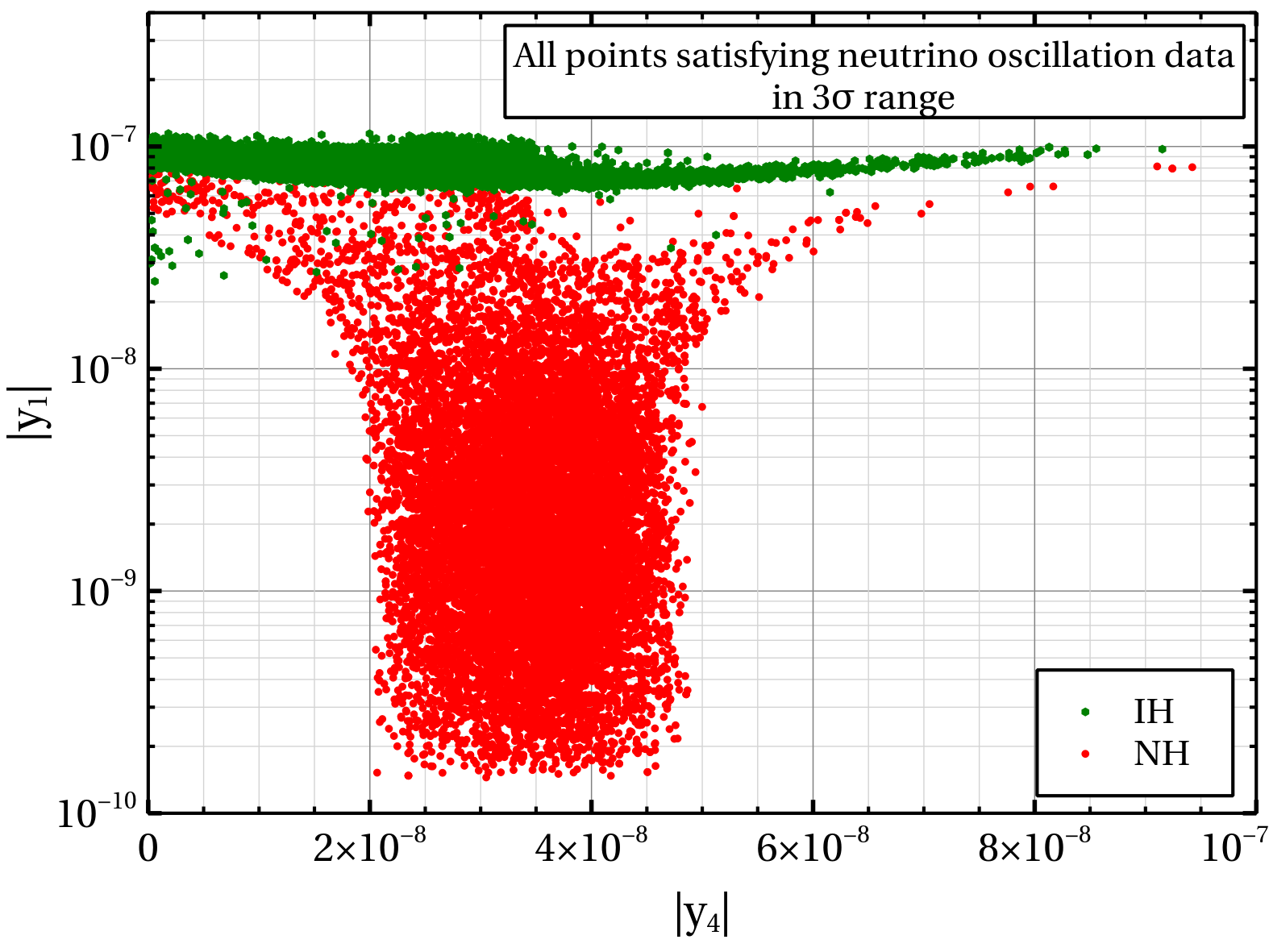
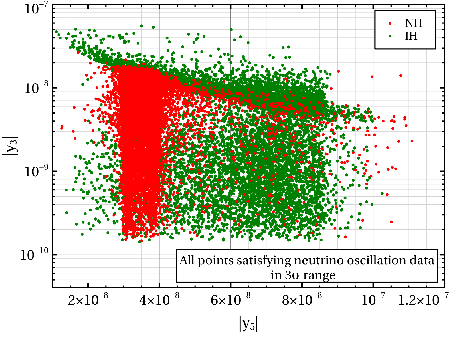
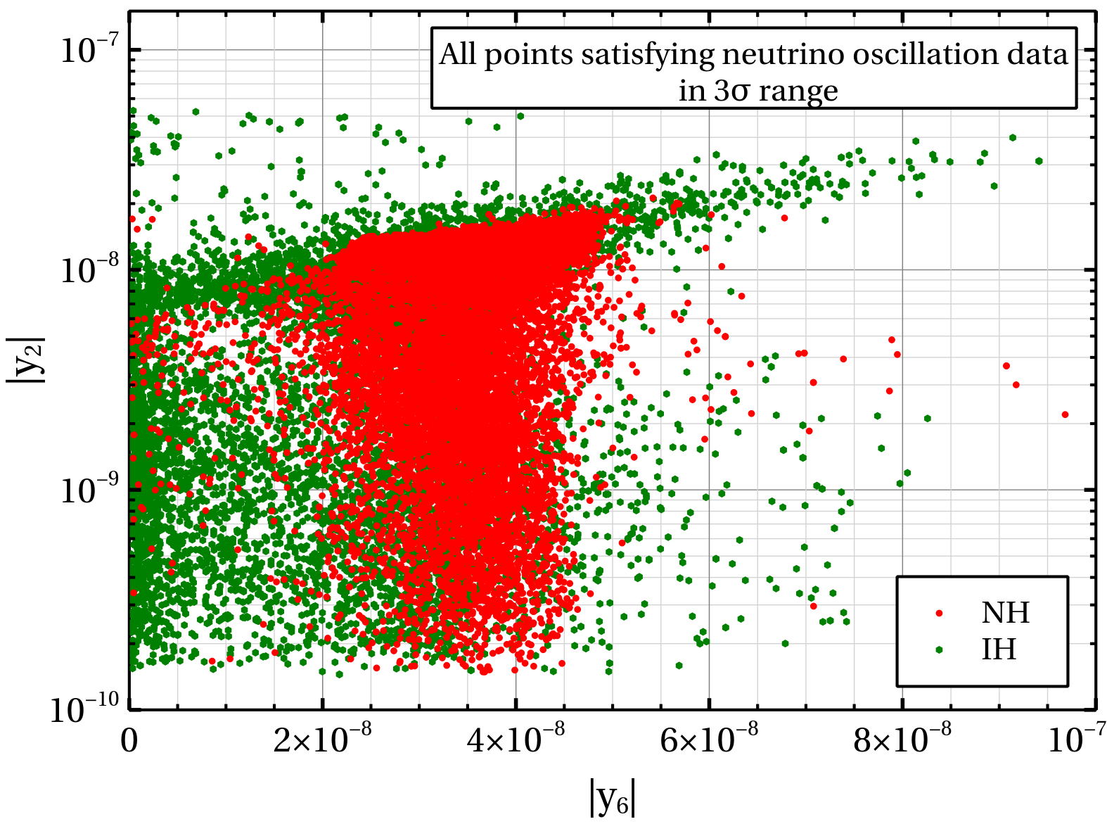
Figure 1: Allowed ranges of absolute values of Yukawa couplings satisfying neutrino oscillation data in 3$\sigma$ limit for both normal (red coloured region) and inverted (green coloured region) hierarchies. All three plots have been generated for $v_{t}=10^{-3}$ GeV.

In order to obtain the allowed values of Yukawa couplings, defined in Eq. 61, we have diagonalised the neutrino mass matrix Eq. 68 following the diagonalisation procedure given in Ref. Adhikary:2013bma and find the physical masses and intergenerational mixing angles of SM neutrinos. The corresponding ranges for the absolute values of Yukawa couplings which reproduce the neutrino oscillation data in $3\sigma$ range and other experimental results as well (mentioned above) are shown in all the three panels of Fig. 1. The red coloured patches in Fig. 1 representing the allowed regions for the normal hierarchical scenario while the green coloured regions are for the inverted mass ordering of neutrinos. All three plots of Fig. 1 and also other plots in the present section (Section III) have been generated for the triplet scalar VEV $v_{t}=10^{-3}$ GeV.

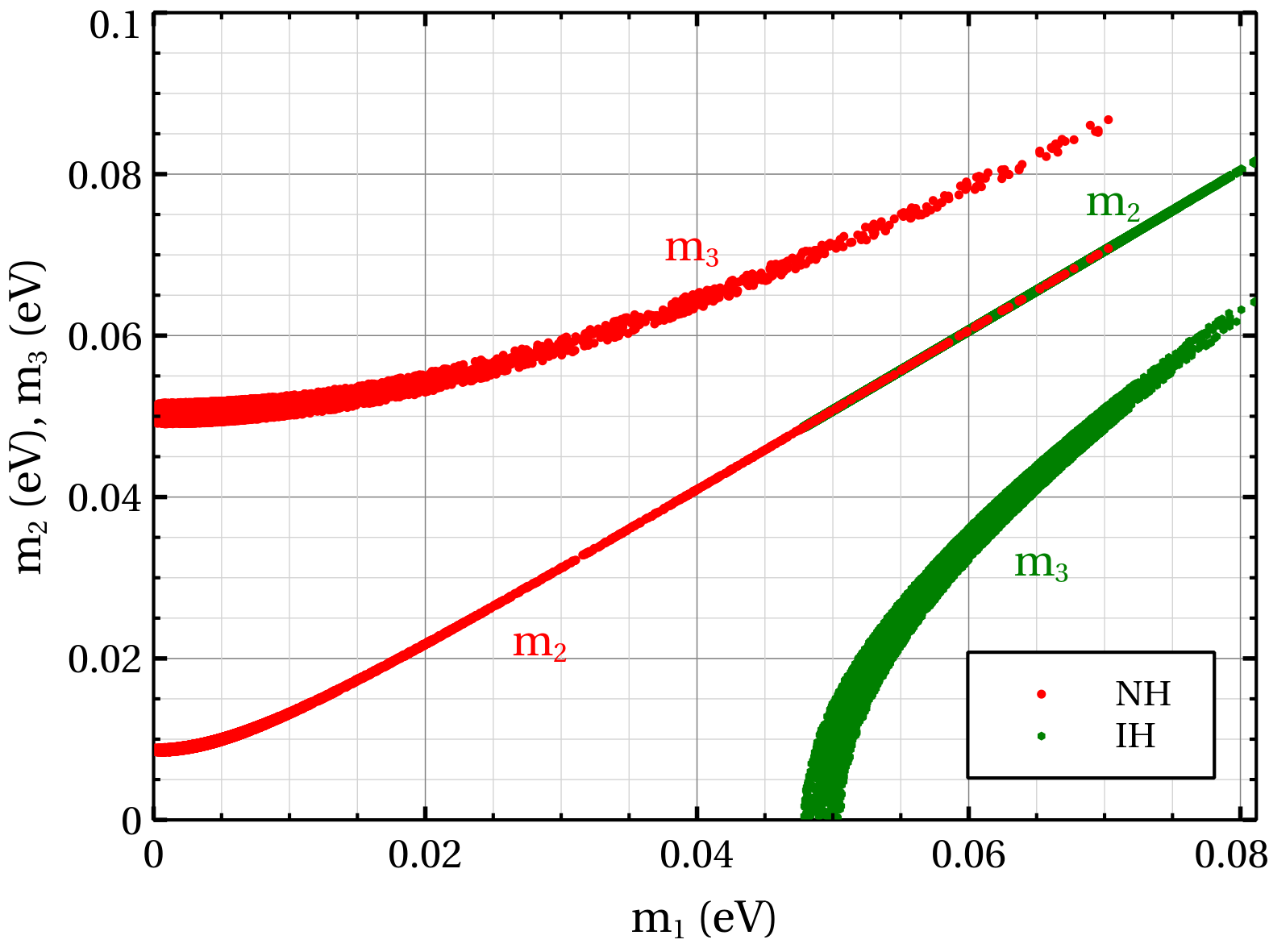
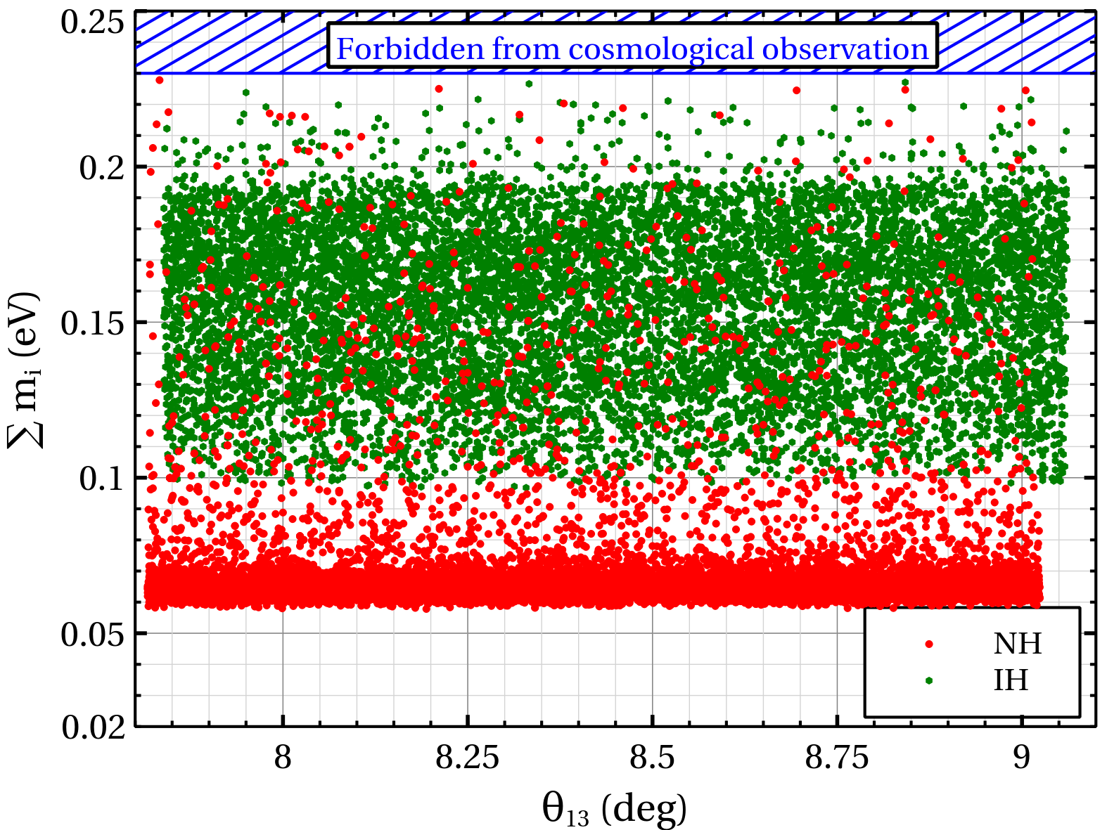
Figure 2: Left panel: Absolute values of neutrino masses allowed by neutrino oscillation data. Right panel: Allowed values of $\sum m_{i}$ with respected to the measured values of $\theta_{13}$.

In the left panel of Fig. 2, we show the absolute values of neutrino masses allowed from the neutrino oscillation data for both normal (red coloured points) and inverted (green coloured points) hierarchies. As the solar neutrino data suggests extremely small splitting between $m_{2}$ and $m_{1}$ ($\Delta m^{2}_{21}\sim 10^{-5}$ eV²), the $m_{1}-m_{2}$ parameter space is very narrow and almost aligned along the line $m_{1}=m_{2}$ for both hierarchical scenarios. Moreover, as expected for the case of inverted mass ordering ($m_{2}\mathrel{\mathchoice{\vbox{\offinterlineskip\halign{\hfil$\displaystyle#$\hfil\cr>\cr\sim\cr}}}{\vbox{\offinterlineskip\halign{\hfil$\textstyle#$\hfil\cr>\cr\sim\cr}}}{\vbox{\offinterlineskip\halign{\hfil$\scriptstyle#$\hfil\cr>\cr\sim\cr}}}{\vbox{\offinterlineskip\halign{\hfil$\scriptscriptstyle#$\hfil\cr>\cr\sim\cr}}}}m_{1}>m_{3}$), the allowed values of $m_{1}$ is larger compared to that of normal mass ordering ($m_{3}>m_{2}\mathrel{\mathchoice{\vbox{\offinterlineskip\halign{\hfil$\displaystyle#$\hfil\cr>\cr\sim\cr}}}{\vbox{\offinterlineskip\halign{\hfil$\textstyle#$\hfil\cr>\cr\sim\cr}}}{\vbox{\offinterlineskip\halign{\hfil$\scriptstyle#$\hfil\cr>\cr\sim\cr}}}{\vbox{\offinterlineskip\halign{\hfil$\scriptscriptstyle#$\hfil\cr>\cr\sim\cr}}}}m_{1}$). Furthermore, from the left panel of Fig. 2, it is also seen that for NH, the allowed values of $m_{3}$ lie above the line $m_{1}=m_{3}$ in $m_{1}-m_{3}$ parameter space indicating $m_{3}>m_{1}$ while the exactly opposite nature has been observed for the inverted hierarchical case. In the right panel of Fig. 2, we plot the sum over all three neutrino masses ($\sum m_{i}$) with the allowed values of reactor mixing angle $\theta_{13}$. From this figure one can clearly see that for the normal hierarchical scenario, $\sum m_{i}$ in the present case is mainly concentrated around $\sim$ 0.06 eV to 0.1 eV. On the other hand, the sum of all three neutrino masses for the inverted ordering mostly lie between 0.1 eV to 0.2 eV. The blue dashed region corresponds to $\sum m_{i}>0.23$ eV which is excluded from the cosmological observation at 95% C.L. Also, in the present model irrespective of neutrino mass ordering, we find that $\sum m_{i}$ is uniformly distributed over the entire experimentally allowed values of $\theta_{13}$.

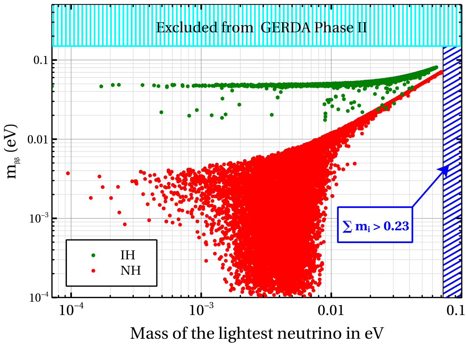
Figure 3: Left panel: Variation of effective neutrino mass parameter with mass of the lightest neutrino for both normal and inverted hierarchies. Right panel: Predicted values of $J_{CP}$ and $\delta$ from the present model. Current limits on $\delta$ from the T2K experiment are indicated by the dashed regions.

Variation of effective Majorana mass $m_{\beta\beta}$ with respect to the lightest neutrino mass has been shown in the left panel of Fig. 3. The effective Majorana mass parameter $m_{\beta\beta}=\left|\sum_{k}m_{k}\,(U_{\rm PMNS})^{2}_{1k}\right|=(M_{\nu})_{11}$ is an important quantity as it enters into the expression of lifetime of neutrinoless double $\beta$ decay i.e. $2n\rightarrow 2p+2e^{-}$. This process violates lepton number by 2 units and is possible only if the neutrinos are Majorana fermions. Like the previous plots, here also we have indicated the values of $m_{\beta\beta}$ by red(green) coloured points for NH(IH) in $m_{1(3)}-m_{\beta\beta}$ plane. The most stringent bound on $m_{\beta\beta}$ comes from GERDA phase II experiments which has reported an upper bound on the effective Majorana mass $m_{\beta\beta}<0.15-0.33$ eV at 90% C.L. Agostini:2017iyd . This upper bound on $m_{\beta\beta}$ has been shown by the turquoise dashed region in $m_{1(3)}-m_{\beta\beta}$ plane while the blue dashed region indicating the upper bound on the mass of the lightest neutrino $m_{1}\mathrel{\mathchoice{\vbox{\offinterlineskip\halign{\hfil$\displaystyle#$\hfil\cr<\cr\sim\cr}}}{\vbox{\offinterlineskip\halign{\hfil$\textstyle#$\hfil\cr<\cr\sim\cr}}}{\vbox{\offinterlineskip\halign{\hfil$\scriptstyle#$\hfil\cr<\cr\sim\cr}}}{\vbox{\offinterlineskip\halign{\hfil$\scriptscriptstyle#$\hfil\cr<\cr\sim\cr}}}}0.0713$ eV (for NH) obtained by combining the cosmological upper limit on $\sum m_{i}$ and neutrino oscillation data. Moreover, from this plot it also appears that the allowed values of $m_{\beta\beta}$ for IH are larger compared to that of NH. This can be understood from the right panel of Fig. 2, where one can easily see that for most of the allowed region of $\theta_{13}$, the values of $\sum m_{i}$ are larger for the case of inverted mass ordering. Consequently, the effective Majorana mass parameter $m_{\beta\beta}=\left|\sum_{k}m_{k}\,(U_{\rm PMNS})^{2}_{1k}\right|$ for IH appears to be large as the elements of $U_{\rm PMNS}$ matrix are nearly identical for both the mass hierarchies. Furthermore, since the effective Majorana mass parameter is related to the $(1,1)$ elements of neutrino mass matrix $M_{\nu}$, absolute values of the Yukawa coupling $y_{1}$ ($(1,1)$ element of $M_{\nu}$, Eq. 68) are large for IH and mainly concentrated around $\sim 10^{-7}$ (see left most plot of Fig. 1).

In the right panel of Fig. 3, we show the predicted values of $J_{\rm CP}$ and Dirac CP phase $\delta$ from the present model, which have been computed using the relevant model parameters satisfying neutrino oscillation data and other experimental bounds mentioned above. From this plot it is clearly seen the Dirac CP phase $\delta$ has two allowed regions regardless of neutrino mass hierarchies. However, for the normal ordering the predicted ranges of $\delta$ are larger compared to that for the inverted mass ordering. For NH, $\delta$ spans the entire first and fourth quadrant while it lies between $90^{\circ}-140^{\circ}$ and $220^{\circ}-270^{\circ}$ for IH. Recently T2K experiment has reported a 90% C.L. allowed region for $\delta$ which is $200.20^{\circ}<\delta<316.23^{\circ}$($228.45^{\circ}<\delta<329.98^{\circ}$) for normal(inverted) mass ordering Abe:2017vif . In the right panel of Fig. 3, these results have been indicated by the blue and pink dashed regions respectively. This plot indicates that the T2K results prefer the values of Dirac CP phase $\delta$ lying in the third and fourth quadrant instead of other two remaining quadrants. Moreover, for these values of $\delta$ we have also computed $J_{CP}$ and from the right panel of Fig. 3 one can easily notice that irrespective of neutrino mass ordering the absolute values of $J_{CP}$ always lie below 0.039 Petcov:2013poa .

On top of these, the neutrino mixing matrix ($U_{\rm PMNS}$, Eq. 72) introduces flavour violating decays in the leptonic sector such as $\mu\rightarrow e\,\gamma$ etc., which remain absent in the SM and occur at one loop level in the present model due to contributions from virtual $W^{\pm}$, $H^{\pm}$ and $H^{\pm\pm}$ loops. The expression for the Branching ratio of $\mu\rightarrow e\,\gamma$ in the present scenario is given by 1205.4671 ,

$${\rm BR}(\mu\rightarrow e\,\gamma) \simeq \dfrac{\Gamma(\mu\rightarrow e\,\gamma)}{\Gamma(\mu\rightarrow e\,\nu_{\mu}\,\bar{\nu}_{e})}\,,$$ (77)

$$= \dfrac{\alpha_{\rm em}}{48\,\pi}\dfrac{\left|\left(M^{\dagger}_{\nu}\,M_{\nu}\right)_{e\,\mu}\right|^{2}}{G_{F}^{2}\,v^{4}_{t}}\,\left(\dfrac{1}{M^{2}_{H^{\pm}}}+\dfrac{8}{M^{2}_{H^{\pm\pm}}}\right)^{2}\,,$$

where $G_{F}$ is the Fermi constant and $\alpha_{\rm em}=\dfrac{{\bf e}^{2}}{4\,\pi}$, ${\bf e}$ being the magnitude of electric charge of electron. The non-observation of this flavour violating decay imposes a strong upper limit on the branching ratio of this decay mode. Currently the most stringent upper bound on ${\rm BR}(\mu\rightarrow e\,\gamma)$ has been reported by the MEG collaboration TheMEG:2016wtm which is ${\rm BR}(\mu\rightarrow e\,\gamma)<4.2\times 10^{-13}$ at 90% C.L. We have checked that for our allowed parameter space, which reproduces the neutrino oscillation data and also satisfies all the other relevant constraints considered in this section, the quantity ${\rm BR}(\mu\rightarrow e\,\gamma)$ comes out to be many orders of magnitude less than the present experimental bound.

IV Dark Matter

We have already mentioned in the Section II that besides the usual SM gauge symmetry we have introduced an additional $\mathbb{Z}_{2}$ symmetry in the present model. Under this newly added $\mathbb{Z}_{2}$ symmetry all the fields present in the model except $\Phi$ are even. Moreover, since the doublet $\Phi$ does not acquire any VEV, $\mathbb{Z}_{2}$ symmetry remains preserved i.e. all the interactions are $\mathbb{Z}_{2}$ conserving. This automatically ensures that all heavier $\mathbb{Z}_{2}$ odd particles will decay to the lightest odd particle (LOP). Hence, the LOP becomes naturally stable over the cosmological time scale and can be treated as a viable dark matter candidate of the Universe. In the present scenario anyone between the two neutral components of $\Phi$ namely, $\phi^{0}$, $a^{0}$ can be an LOP. For definiteness, in this work we have considered $\phi^{0}$ as LOP. Now to test the viability of $\phi^{0}$ as a cold dark matter candidate, the primary task is to calculate its relic abundance at the present epoch. In order to compute the relic abundance of a thermal dark matter candidate, we need to solve the Boltzmann equation involving comoving number density $Y_{i}=\dfrac{n_{\phi^{0}}}{\rm s}$, where $n_{i}$ is the actual number density of a species $i$ while ${\rm s}$ is the entropy density of the Universe. The relevant Boltzmann equation for the computation of comoving number density of dark matter at the present epoch is given byGriest:1990kh ; Edsjo:1997bg ,

$$\dfrac{dY}{dx}=-\left(\dfrac{45\,G}{\pi}\right)^{-\frac{1}{2}}\dfrac{M_{\phi^{0}}\,\sqrt{g_{\star}}}{x^{2}}\sum_{i\,j}\langle{\sigma_{i\,j}{\rm v}_{i\,j}}\rangle\,(Y_{i}\,Y_{j}-Y_{i}^{\rm eq}\,Y_{j}^{\rm eq})\,,$$ (78)

where $Y=\sum_{i}Y_{i}$ is the comoving number density of dark matter and the summation is over all three $\mathbb{Z}_{2}$ odd particles, i.e. $\phi^{+}$, $a^{0}$ and $\phi^{0}$. The dimensionless variable $x$ is defined as $x=\dfrac{M_{\phi^{0}}}{T}$, where $M_{\phi^{0}}$ is the mass of the LOP $\phi^{0}$ and $T$ is the temperature of the Universe. The expression for the mass of $\phi^{0}$ in terms of parameters appearing in the Lagrangian is given in Eq. 17. Moreover, $G=M^{-2}_{pl}$ is the Newton’s gravitational constant and $M_{pl}=1.22\times 10^{19}$ GeV, is the Planck mass. The expression of $g_{\star}$ is given by

$$\sqrt{g_{\star}}=\dfrac{{g_{\rm s}}}{\sqrt{g_{\rho}}}\left(1+\dfrac{1}{3}\,\dfrac{d\ln g_{\rm s}}{d\ln T}\right)\,,$$ (79)

where $g_{\rm s}$ and $g_{\rho}$ are degrees of freedom related to the entropy density (${\rm s}$) and energy density ($\rho$) of the Universe.

Now, the above Eq. 78 will be in a simplified form, if we use an approximation $\dfrac{Y_{i}}{Y}\simeq\dfrac{Y^{\rm eq}_{i}}{Y^{\rm eq}}$ Griest:1990kh ; Edsjo:1997bg i.e. the fraction of a species $i$ to the total comoving number density $Y$ of odd sector particles always maintains its equilibrium value. Using this relation, the Boltzmann equation can be written in the following form Griest:1990kh ; Edsjo:1997bg

$$\dfrac{dY}{dx}=-\left(\dfrac{45\,G}{\pi}\right)^{-\frac{1}{2}}\dfrac{M_{\phi^{0}}\,\sqrt{g_{\star}}}{x^{2}}\langle{\sigma{\rm v}}\rangle_{\rm eff}\,(Y^{2}-(Y^{\rm eq})^{2})\,.$$ (80)

The quantity $\langle{\sigma{\rm v}}\rangle_{\rm eff}$ is defined as

$$\langle{\sigma{\rm v}}\rangle_{\rm eff}=\sum_{i\,j}\langle{\sigma_{i\,j}{\rm v}_{i\,j}}\rangle\times r_{i}\,r_{j}\,,$$ (81)

where

$$r_{i}=\dfrac{Y^{\rm eq}_{i}}{Y}=\dfrac{n^{\rm eq}_{i}}{n}=\dfrac{g_{i}\left(1+\Delta_{i}\right)^{3/2}\exp[-\Delta_{i}\,x]}{\sum_{i}g_{i}\left(1+\Delta_{i}\right)^{3/2}\exp[-\Delta_{i}\,x]}\,.$$ (82)

Here $\Delta_{i}=\dfrac{M_{i}-M_{\phi^{0}}}{M_{\phi^{0}}}$, $g_{i}$ is the internal degrees of freedom of odd sector particle $i$ ($i=\phi^{\pm},\,a^{0},\,\phi^{0}$) and $n=\sum_{i}n_{i}$ is the total number density of $\mathbb{Z}_{2}$ odd particles. For equilibrium number density $n^{\rm eq}_{i}$ of a species $i$, one can use the Maxwell Boltzmann distribution. Finally, the quantity $\langle{\sigma_{i\,j}{\rm v}_{i\,j}}\rangle$ in the above equations represents the thermally averaged annihilation cross section between the odd sector particles and ${\rm v}_{i\,j}$ is the relative velocity between the two annihilating initial state particles. For two identical initial state particles ($i=j$), $\sigma_{ii}$ denotes the self-annihilation cross section of a species $i$ to all possible final state particles allowed by the symmetries of the Lagrangian while the co-annihilation between these particles occurs when annihilating particles are not identical i.e. $i\neq j$. Besides the self annihilation processes of LOP ($i=j=\phi^{0}$), the co-annihilation between an odd sector particle $i$ and LOP as well as the self annihilation of the species $i$ will have a significant effect on dark matter relic abundance at the present epoch if the mass splitting between LOP and other odd sector particle $i$ is very small i.e. $\Delta_{i}=\dfrac{M_{i}-M_{\phi^{0}}}{M_{\phi^{0}}}<0.1$ Griest:1990kh . The expression of $\langle{\sigma_{i\,j}{\rm v}_{i\,j}}\rangle$ is given by Biswas:2016yjr

$$\langle{\sigma_{i\,j}{\rm v}_{i\,j}}\rangle=\frac{1}{8\,M^{2}_{i}\,M^{2}_{j}\,T\,{\rm K}_{2}\left(\dfrac{M_{i}}{T}\right)\,{\rm K}_{2}\left(\dfrac{M_{j}}{T}\right)}\times\int^{\infty}_{(M_{i}+M_{j})^{2}}\dfrac{\sigma_{ij}}{\sqrt{s}}\,f_{1}\,f_{2}\,{\rm K}_{1}\left(\frac{\sqrt{s}}{T}\right)\,ds\,,$$ (83)

with

$$f_{1}=\sqrt{s^{2}+(M^{2}_{i}-M^{2}_{j})^{2}-2\,s\,(M^{2}_{i}+M^{2}_{j})}\,,$$

$$f_{2}=\sqrt{s-(M^{2}_{i}-M^{2}_{j})^{2}}\sqrt{s-(M^{2}_{i}+M^{2}_{j})^{2}}\,.$$ (84)

In the above, $s$ is the Mandelstam variable and ${\rm K}_{i}$ is the $i$th order Modified Bessel function of second kind. All the relevant couplings required to calculate $\sigma_{i\,j}$ are given in Appendix C. To compute relic density of dark matter we need the value of comoving number density $Y$ at the present epoch $T=T_{0}$, which can be found by solving the Boltzmann equation given in Eq. 80. We have solved this equation using micrOMEGAs Belanger:2014vza package where the information about the present model has been implemented using FeynRules Alloul:2013bka package. After finding the value of $Y(T_{0})$, the dark matter relic density can now be obtained from the following relation Edsjo:1997bg

$$\Omega h^{2}=2.755\times 10^{8}\,\left(\dfrac{M_{\phi^{0}}}{\rm GeV}\right)\,Y(T_{0})\,.$$ (85)

In addition to all the theoretical as well as experimental constraints mentioned in previous sections, we have also considered few more experimental bounds which are indispensable to the dark matter phenomenology. These are discussed below,

• Relic density of dark matter: Various satellite borne experiments viz. WMAP Hinshaw:2012aka , Planck Ade:2015xua have precisely measured the abundance of dark matter in the Universe at the present epoch, which is

  $$0.1172\leq\Omega h^{2}\leq 0.1226\,\,\,\,{\rm at}\,\,68\%\,\,{\rm C.L.}\,.$$ (86)

• Spin independent elastic scattering cross section: In the present model dark matter candidate $\phi^{0}$ can elastically scatter off the terrestrial detector nuclei by exchanging CP even scalar bosons $h^{0}$ and $H^{0}$. This is known as the spin independent elastic scattering cross section of $\phi^{0}$ which is assumed to be responsible for its direct signature in the earth based detectors. The spin independent elastic scattering cross section for the process $\phi^{0}+N\rightarrow\phi^{0}+N$ with $N$ being a nucleon is given by

  $$\sigma_{\rm SI}=\dfrac{\mu^{2}_{\rm red}}{4\pi}\left[\dfrac{M_{N}\,f_{N}}{M_{\phi^{0}}\,v_{d}}\left(\dfrac{\,g_{\phi^{0}\phi^{0}h^{0}}}{M^{2}_{h^{0}}}-\dfrac{\,g_{\phi^{0}\phi^{0}H^{0}}}{M^{2}_{H^{0}}}\right)\right]^{2}\,,$$ (87)

  where $\mu_{\rm red}=\frac{M_{N}M_{\phi^{0}}}{M_{N}+M_{\phi^{0}}}$ is the reduced mass of nucleon $N$ and $\phi^{0}$ while $f_{N}$ is the nuclear form factor for scalar mediated interactions and its value is $\sim 0.3$ 1306.4710 . In Eq. 87, the negative sign arises due to the opposite sign of couplings of $h^{0}$ and $H^{0}$ with quarks $q$ (i.e. $h^{0}(H^{0})\bar{q}q$ coupling). The coupling between two dark matter particles and a CP even scalar $h^{0}$($H^{0}$) is represented by $g_{\phi^{0}\phi^{0}h^{0}(H^{0})}$, which can be decomposed into two parts. One is coming form the $\mathbb{Z}_{2}$ even doublet $H$ while other part is from the triplet $\Delta$. These coupling can be written as

  $$g_{\phi^{0}\phi^{0}h^{0}} = -\bar{\lambda}_{1}\,v_{d}-\bar{\lambda}_{2}\,v_{t}\,,$$ (88)

  $$g_{\phi^{0}\phi^{0}H^{0}} = \tilde{\lambda}_{1}\,v_{d}-\tilde{\lambda}_{2}\,v_{t}\,,$$ (89)

  with

  $$\bar{\lambda}_{1} = \left(\lambda_{5}+\lambda_{6}+2\lambda_{9}\right)\,\cos\alpha\,,$$ (90)

  $$\bar{\lambda}_{2} = \left(\lambda_{7}+\lambda_{8}-\frac{\sqrt{2}\,\tilde{\mu}}{v_{t}}\right)\,\sin\alpha\,,$$ (91)

  $$\tilde{\lambda}_{1} = \left(\lambda_{5}+\lambda_{6}+2\lambda_{9}\right)\,\sin\alpha\,,$$ (92)

  $$\tilde{\lambda}_{2} = \left(\lambda_{7}+\lambda_{8}-\frac{\sqrt{2}\,\tilde{\mu}}{v_{t}}\right)\,\cos\alpha\,,$$ (93)

  and the quantity $\tilde{\mu}$ can be defined in terms free parameters of the present model as

  $$\tilde{\mu}=\dfrac{(\lambda_{6}+2\lambda_{9})\,v^{2}_{d}+\lambda_{8}v^{2}_{t}+2\,\Delta M^{2}_{\pm}}{2\sqrt{2}\,v_{t}}\,,$$ (94)

  while $\Delta M^{2}_{\pm}$ is the mass squared difference between the LOP and inert charged scalar $\phi^{\pm}$ i.e.

  $$\Delta M^{2}_{\pm}=M^{2}_{\phi^{\pm}}-M^{2}_{\phi^{0}}\,.$$ (95)

  Later, we will see that $g_{\phi^{0}\phi^{0}h^{0}}$ coupling will play a significant role in the freeze-out process for low mass range of $\phi^{0}$ ($\phi^{0}<80$ GeV).

  The non-observation of any dark matter signal in direct detection experiments has severely constrained the dark matter-nucleon spin independent scattering cross section and at present the most stringent bound on $\sigma_{\rm SI}$ has been reported by XENON 1T collaboration Aprile:2017iyp . Therefore, a viable dark matter model requires $\sigma_{\rm SI}<\sigma_{exp}$ where $\sigma_{exp}$ being the upper bound on $\sigma_{\rm SI}$ obtained from the XENON 1T direct detection experiment.

• Lower bounds on BSM scalar masses: Precise measurement of $Z$ boson decay width at LEP ALEPH:2005ab forbids any additional invisible decay modes of $Z$ boson i.e. $Z\rightarrow\phi^{0}\,a^{0}$. This puts a lower bound on the sum of the two masses i.e.

  $$M_{\phi^{0}}+M_{a^{0}}>M_{Z}\,.$$ (96)

  Apart from this, the LEP II data also ruled out a significant portion of odd sector scalar masses which satisfy following inequalities 0810.3924

  $$M_{\phi^{0}}<80\,\,{\rm GeV},M_{a^{0}}<100\,\,{\rm GeV}\,\,{\rm and}\,\,M_{a^{0}}-M_{\phi^{0}}>8\,\,{\rm GeV}\,.$$ (97)

  Moreover, there exists a lower bound of 80 GeV at 95% C.L. Patrignani:2016xqp on charged scalar mass from LEP. Keeping in mind all these experimental results, in this work we have considered the masses of $\phi^{\pm}$ and $a^{0}$ larger than 100 GeV i.e. $M_{\phi^{\pm}}\,,M_{a^{0}}>100$ GeV.

• Invisible decay width of SM Higgs boson: In the present model, since we have $h^{0}\phi^{0}\phi^{0}$ coupling, a pair of $\phi^{0}$ can be produced from the decay of SM-like Higgs boson $h^{0}$ at LHC, if the kinematical condition $M_{h^{0}}\geq 2\,M_{\phi^{0}}$ holds. This non-standard decay channel is known as the invisible decay mode of SM-like Higgs boson. Current experimental lower limits on the masses of $\mathbb{Z}_{2}$ particles allow only one invisible decay mode of $h^{0}$ in the present scenario which is $h^{0}\rightarrow\phi^{0}\phi^{0}$. The decay width of this process is given by

  $$\Gamma_{h^{0}\rightarrow\phi^{0}\phi^{0}}=\dfrac{g^{2}_{h^{0}\rightarrow\phi^{0}\phi^{0}}}{32\pi M_{h^{0}}}\sqrt{1-\dfrac{4\,M^{2}_{\phi^{0}}}{M^{2}_{h^{0}}}}\,.$$ (98)

  Throughout this work we have restricted ourselves to that portion of the parameter space where the invisible decay width of SM-like Higgs boson is less than $20\%$ of its total decay width (invisible branching ratio ${\rm BR}_{\rm inv}<0.2$) Khachatryan:2016whc .

Now, we will present the results of dark matter phenomenology of the present model considering $\phi^{0}$ as our dark matter candidate. In this work, we have varied the mass of $\phi^{0}$ between 10 GeV to 1 TeV. In order to determine the allowed parameter space of this model which will satisfy both theoretical as well as experimental constraints we have scanned the free parameters (mentioned in Eq. 44) in the following ranges

$$\begin{array}[]{cccccc}1.0\times 10^{-5}&\leq&\left|\lambda_{i}\right|\,(i=5-9)&\leq&1.0\,\,,\\ 1.0\times 10^{-4}&\leq&\lambda_{\Phi}&\leq&1.0\,\,,\\ 1.0\times 10^{-6}&\leq&\left|\alpha\right|\,({\rm rad})&<&1.0\times 10^{-2}\,\,,\\ 120&\leq&M_{H^{\pm\pm}}\,\text{(GeV)}&\leq&350\,\,,\\ 110&\leq&M_{H^{\pm}}\,\text{(GeV)}&\leq&330\,\,,\\ 100&\leq&M_{H^{0}}\,\text{(GeV)}&\leq&300\,\,,\\ 10&\leq&M_{\phi^{0}}\,\text{(GeV)}&\leq&1000\,\,,\\ 100&<&M_{\phi^{\pm}}\,\text{(GeV)}&\leq&1050\,,\end{array}$$ (107)

with $M_{\phi^{\pm}}>M_{\phi^{0}}$. Furthermore, in the present scenario mass of the inert CP odd scalar $a^{0}$ is not a free parameter as one can easily express $M_{a^{0}}$ in terms of our chosen free parameters, i.e.

$$M^{2}_{a^{0}}=\lambda_{8}v^{2}_{t}+\lambda_{6}v^{2}_{d}+(2\,M^{2}_{\phi^{\pm}}-M^{2}_{\phi^{0}})\,.$$ (108)

Throughout this work, we have used the condition $M_{a^{0}}>M_{\phi^{0}}$, in other word, $\phi^{0}$ is the lightest particle of the odd sector (LOP). Using the above ranges of model parameters, we have found that the dark matter relic density satisfies the Planck limit ($0.1172\leq\Omega h^{2}\leq 0.1226$ Ade:2015xua ) only in two distinct mass ranges of $\phi^{0}$. One of them is the low mass region where $M_{\phi^{0}}$ lies below 90 GeV ($M_{\phi^{0}}<90$ GeV) while in the high mass region $M_{\phi^{0}}$ is larger than 535 GeV ($M_{\phi^{0}}>535\text{ GeV}$). The allowed region in $M_{\phi^{0}}-\sigma_{\rm SI}$ plane for the low mass range of $\phi^{0}$ is shown Fig. 4. The left panel of Fig. 4 has been generated for the triplet VEV $v_{t}=3$ GeV while the right panel is for $v_{t}=1$ MeV. In both panels, all red colours points in $M_{\phi^{0}}-\sigma_{\rm SI}$ plane satisfy the relic density bound as well as the other theoretical constraints considered in this work like unitarity, vacuum stability etc. The green solid line denotes the most severe upper bounds on the dark matter spin independent scattering cross section till date. This experimental upper limits on $\sigma_{\rm SI}$ has been reported recently by the XENON 1T collaboration Aprile:2017iyp . From both panels of Fig. 4, one can see that the current limits on $\sigma_{\rm SI}$ from XENON 1T have ruled out maximum portion of the region with $M_{\phi^{0}}\mathrel{\mathchoice{\vbox{\offinterlineskip\halign{\hfil$\displaystyle#$\hfil\cr<\cr\sim\cr}}}{\vbox{\offinterlineskip\halign{\hfil$\textstyle#$\hfil\cr<\cr\sim\cr}}}{\vbox{\offinterlineskip\halign{\hfil$\scriptstyle#$\hfil\cr<\cr\sim\cr}}}{\vbox{\offinterlineskip\halign{\hfil$\scriptscriptstyle#$\hfil\cr<\cr\sim\cr}}}}50$ GeV.

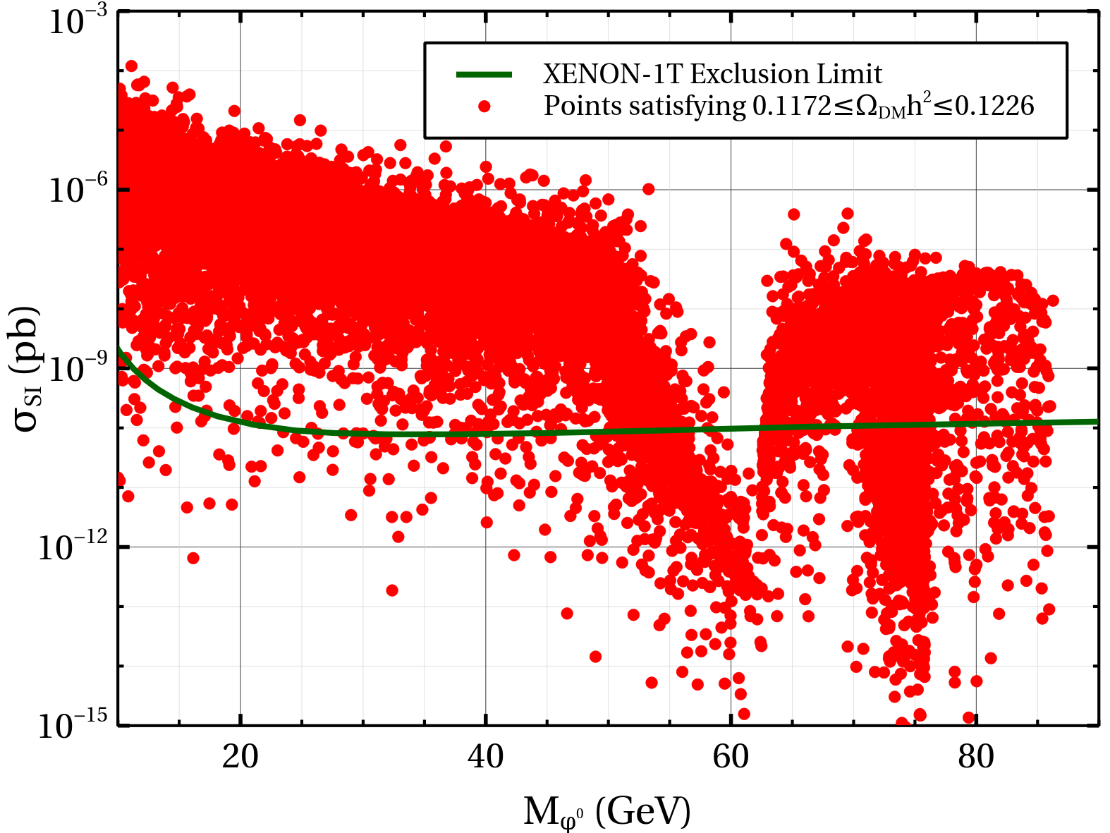
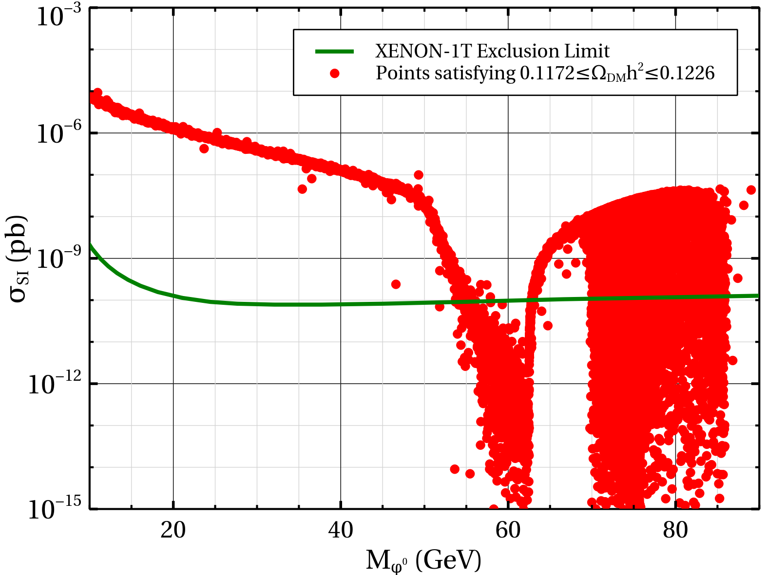
Figure 4: Variation of spin independent scattering cross section $\sigma_{\rm SI}$ with the mass of $\phi^{0}$ for two different values of triplet VEV namely $v_{t}=3$ GeV (left panel) and $v_{t}=1$ MeV (right panel).

Although, for $v_{t}=3$ GeV there are still some allowed parameter space with $M_{\phi^{0}}\mathrel{\mathchoice{\vbox{\offinterlineskip\halign{\hfil$\displaystyle#$\hfil\cr<\cr\sim\cr}}}{\vbox{\offinterlineskip\halign{\hfil$\textstyle#$\hfil\cr<\cr\sim\cr}}}{\vbox{\offinterlineskip\halign{\hfil$\scriptstyle#$\hfil\cr<\cr\sim\cr}}}{\vbox{\offinterlineskip\halign{\hfil$\scriptscriptstyle#$\hfil\cr<\cr\sim\cr}}}}50$ GeV, however those regions will be forbidden if we impose the constraint on invisible branching ratio of the SM-like Higgs boson $h^{0}$ (see Fig. 5). In the low mass region, the dark matter particle $\phi^{0}$ annihilates to SM fermion and antifermion, $W^{+}W^{-}$ pairs. Most of the contribution to $\langle\sigma{\rm v}\rangle$ arises from $\phi^{0}\phi^{0}\rightarrow b\bar{b}$ ($W^{+}W^{-}$) channel for $M_{\phi^{0}}\mathrel{\mathchoice{\vbox{\offinterlineskip\halign{\hfil$\displaystyle#$\hfil\cr<\cr\sim\cr}}}{\vbox{\offinterlineskip\halign{\hfil$\textstyle#$\hfil\cr<\cr\sim\cr}}}{\vbox{\offinterlineskip\halign{\hfil$\scriptstyle#$\hfil\cr<\cr\sim\cr}}}{\vbox{\offinterlineskip\halign{\hfil$\scriptscriptstyle#$\hfil\cr<\cr\sim\cr}}}}70$ GeV ($\mathrel{\mathchoice{\vbox{\offinterlineskip\halign{\hfil$\displaystyle#$\hfil\cr>\cr\sim\cr}}}{\vbox{\offinterlineskip\halign{\hfil$\textstyle#$\hfil\cr>\cr\sim\cr}}}{\vbox{\offinterlineskip\halign{\hfil$\scriptstyle#$\hfil\cr>\cr\sim\cr}}}{\vbox{\offinterlineskip\halign{\hfil$\scriptscriptstyle#$\hfil\cr>\cr\sim\cr}}}}70$ GeV). Since we have always considered $M_{\phi^{\pm}},M_{a^{0}}>100$ GeV, the co-annihilations among the inert sector particles have no significant effect on the dark matter relic density in the low mass region of $\phi^{0}$. The sudden dip in $\sigma_{\rm SI}$ around $M_{\phi^{0}}\simeq 60$ GeV is due to the resonance effect of SM-like Higgs boson $h^{0}$ of mass 125.5 GeV. In the resonance region of $h^{0}$ ($M_{\phi^{0}}\sim M_{h^{0}}/2$), the annihilation cross section of $\phi^{0}$ mediated by $h^{0}$ increases sharply, which has an inverse effect on $\Omega h^{2}$. Hence, to generate dark matter relic density within the desired ballpark of Plank limit, the $\phi^{0}\phi^{0}h^{0}$ coupling (defined in Eq. 88) has to be decreased accordingly. As the same coupling also enters into the expression of $\sigma_{\rm SI}$ (see Eq. 87), there exits a sharp decrease in $\sigma_{\rm SI}$ around the resonance region of $h^{0}$.

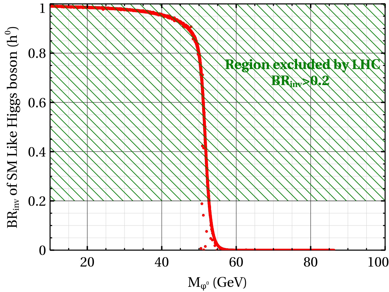
Figure 5: Variation of invisible branching ratio of SM-like Higgs boson $h^{0}$ with the mass of LOP $\phi^{0}$.

It has been already mentioned that in the present scenario, the only source of invisible decay mode of $h^{0}$ is $h^{0}\rightarrow\phi^{0}\phi^{0}$. Therefore, in Fig. 5 invisible branching ratio of the SM-like Higgs boson has been plotted with respect to the mass of $\phi^{0}$. Here the green dashed region represents ${\rm BR}_{\rm inv}\geq 0.2$, which is excluded by the current LHC data Khachatryan:2016whc . All the red points in $M_{\phi^{0}}-{\rm BR}_{\rm inv}$ plane reproduce the dark matter relic density within the allowed ballpark of the Planck limit. It is also evident from Fig. 5 that initially when $M_{\phi^{0}}<40$ GeV, the invisible branching ratio of $h^{0}$ is very high and thereafter there is a sharp fall of ${\rm BR}_{\rm inv}$ for $M_{\phi^{0}}$ lying between 40 GeV to 60 GeV. This nature of ${\rm BR}_{\rm inv}$ is due to the phase space suppression i.e. the available phase space for this decay mode deceases as the mass of $\phi^{0}$ increases and eventually when $M_{\phi^{0}}$ becomes larger than $M_{h^{0}}/2\sim 62.5$ GeV the decay mode $h^{0}\rightarrow\phi^{0}\phi^{0}$ becomes kinematically forbidden and hence ${\rm BR}_{\rm inv}$ of $h^{0}$ vanishes. Most importantly, from this plot it is clearly evident that the dark matter mass $M_{\phi^{0}}\mathrel{\mathchoice{\vbox{\offinterlineskip\halign{\hfil$\displaystyle#$\hfil\cr<\cr\sim\cr}}}{\vbox{\offinterlineskip\halign{\hfil$\textstyle#$\hfil\cr<\cr\sim\cr}}}{\vbox{\offinterlineskip\halign{\hfil$\scriptstyle#$\hfil\cr<\cr\sim\cr}}}{\vbox{\offinterlineskip\halign{\hfil$\scriptscriptstyle#$\hfil\cr<\cr\sim\cr}}}}50$ GeV is excluded by the invisible decay width constraint of $h^{0}$.

Next, in order to illustrate the effects of some relevant parameters on dark matter relic density, we show the variation of $\Omega h^{2}$ with respect to the mass of $\phi^{0}$ in Fig. 6 for three different values of model parameters namely $\alpha$, $\bar{\lambda}_{1}$ and $\bar{\lambda}_{2}$ respectively. In each panel of Fig. 6, three lines represent the variation of relic density for three different values of a chosen model parameter while the horizontal black solid line denotes the central value of dark matter relic density i.e. $\Omega h^{2}=0.1199$ as observed by the Planck satellite. In the leftmost panel, we have considered three different values of CP even scalar mixing angle $\alpha=2.0\times 10^{-4}$ (red dashed line), $1.2\times 10^{-3}$ (green dashed dot line) and $2.0\times 10^{-3}$ (blue dashed dot dot line) respectively. The values of other free parameters have been kept fixed at $M_{H^{\pm\pm}}=156.90$ GeV, $M_{H^{\pm}}=203.39$ GeV, $M_{H^{0}}=M_{A^{0}}=241.03$ GeV, $\Delta M_{\pm}=150$ GeV, $\lambda_{\Phi}=0.0203$, $\lambda_{5}=0.02$, $\lambda_{6}=0.4\times 10^{-4}$, $\lambda_{7}=0.41\times 10^{-3}$, $\lambda_{8}=-0.646\times 10^{-2}$, $\lambda_{9}=0.4\times 10^{-4}$ and $v_{t}=3$ GeV.

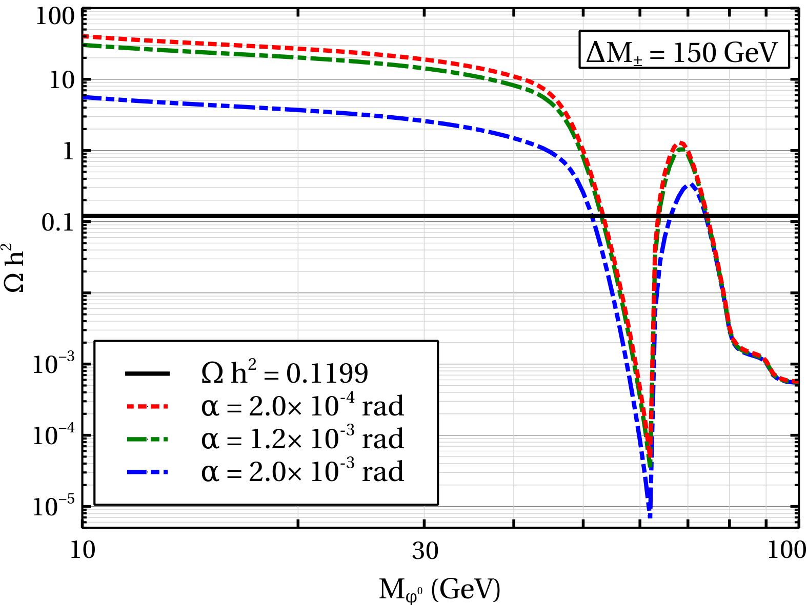
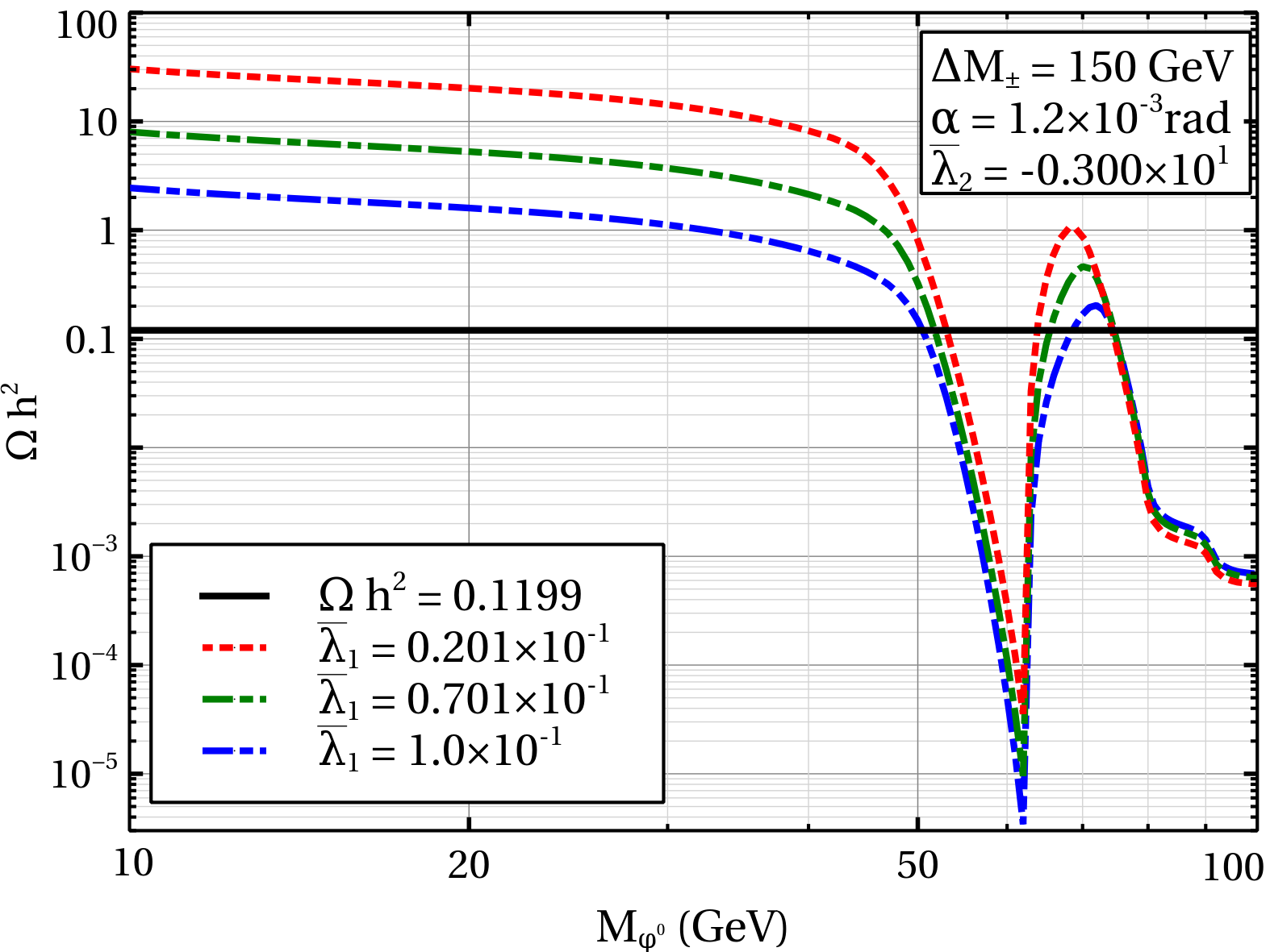
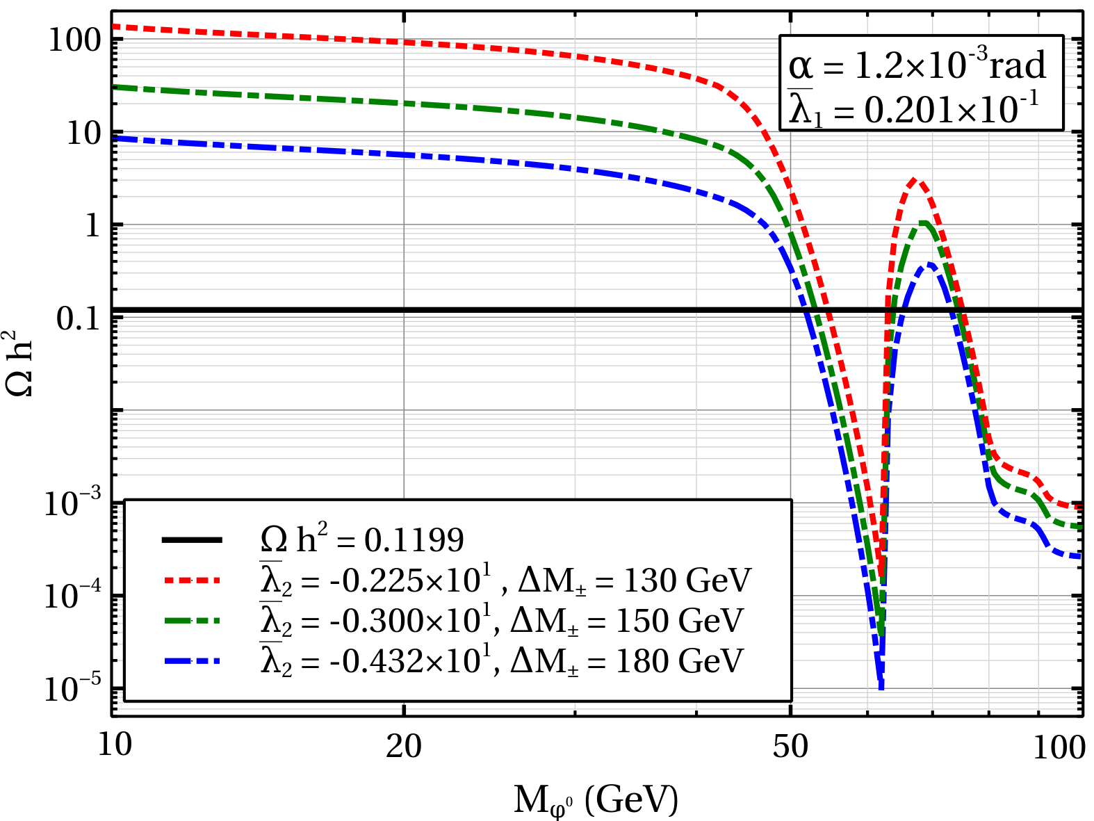
Figure 6: Variation of $\Omega h^{2}$ with $M_{\phi^{0}}$ for three different values of model parameters namely, $\alpha$ (left panel), $\bar{\lambda}_{1}$ (central panel) and $\bar{\lambda}_{2}$ (right panel).

From the leftmost panel one can see that relic density decreases when we increase $\alpha$. This can be understood in the following way. As mentioned earlier, in the low dark matter mass region where $M_{\phi^{0}}\mathrel{\mathchoice{\vbox{\offinterlineskip\halign{\hfil$\displaystyle#$\hfil\cr<\cr\sim\cr}}}{\vbox{\offinterlineskip\halign{\hfil$\textstyle#$\hfil\cr<\cr\sim\cr}}}{\vbox{\offinterlineskip\halign{\hfil$\scriptstyle#$\hfil\cr<\cr\sim\cr}}}{\vbox{\offinterlineskip\halign{\hfil$\scriptscriptstyle#$\hfil\cr<\cr\sim\cr}}}}70$ GeV, the main annihilation channel is $\phi^{0}\phi^{0}\rightarrow b\bar{b}$ mediated by the SM-like Higgs boson $h^{0}$. The coupling $g_{\phi^{0}\phi^{0}h^{0}}$ (Eq. 88) has two parts one of them is proportional to $\cos\alpha$ while other part has $\sin\alpha$. In this plot we have varied $\alpha$ between $2.0\times 10^{-4}$ rad to $2.0\times 10^{-3}$ rad. In this small range of $\alpha$, the coupling $g_{\phi^{0}\phi^{0}h^{0}}$ as well as $\langle\sigma{\rm v}\rangle$ increase with $\alpha$ and hence the relic density behaves oppositely as it is inversely proportional to $\langle\sigma{\rm v}\rangle$. However, beyond the $h^{0}$ resonance region i.e for $M_{\phi^{0}}\mathrel{\mathchoice{\vbox{\offinterlineskip\halign{\hfil$\displaystyle#$\hfil\cr>\cr\sim\cr}}}{\vbox{\offinterlineskip\halign{\hfil$\textstyle#$\hfil\cr>\cr\sim\cr}}}{\vbox{\offinterlineskip\halign{\hfil$\scriptstyle#$\hfil\cr>\cr\sim\cr}}}{\vbox{\offinterlineskip\halign{\hfil$\scriptscriptstyle#$\hfil\cr>\cr\sim\cr}}}}70$ GeV, $\phi^{0}\phi^{0}\rightarrow W^{+}W^{-}$ becomes the main annihilation channel and in this case dominant contribution comes from the diagrams mediated by $H^{0}$ instead of $h^{0}$. The coupling $g_{\phi^{0}\phi^{0}H^{0}}$ has exactly opposite angular dependence compared to $g_{\phi^{0}\phi^{0}h^{0}}$ (Eq. 89). Now for the considered values of model parameters $\left|\left(\lambda_{7}+\lambda_{8}-\dfrac{\sqrt{2}\,\tilde{\mu}}{v_{t}}\right)\right|>>\left|\left(\lambda_{5}+\lambda_{6}+2\,\lambda_{9}\right)\right|$, hence the dominant process becomes practically independent of $\alpha$. As a result we have not observed any significant change in $\Omega h^{2}$ for three different values of $\alpha$ when $M_{\phi^{0}}\mathrel{\mathchoice{\vbox{\offinterlineskip\halign{\hfil$\displaystyle#$\hfil\cr>\cr\sim\cr}}}{\vbox{\offinterlineskip\halign{\hfil$\textstyle#$\hfil\cr>\cr\sim\cr}}}{\vbox{\offinterlineskip\halign{\hfil$\scriptstyle#$\hfil\cr>\cr\sim\cr}}}{\vbox{\offinterlineskip\halign{\hfil$\scriptscriptstyle#$\hfil\cr>\cr\sim\cr}}}}70$ GeV. Similarly, the effects of $\bar{\lambda}_{1}$ and $\bar{\lambda}_{2}$ on $\Omega h^{2}$ can be easily understood using Eqs. 88-93. One should note that in the present model the parameter $\tilde{\mu}$ (defined in Eq. 94) has a profound effect on relic density, e.g. for the particular benchmark point both the couplings $g_{\phi^{0}\phi^{0}h^{0}}$ and $g_{\phi^{0}\phi^{0}H^{0}}$ enhance with the $\tilde{\mu}$ for $10\text{ GeV}\leq M_{\phi^{0}}\leq 100\text{ GeV}$ while $\tilde{\mu}$ itself increases with $\Delta M_{\pm}$.

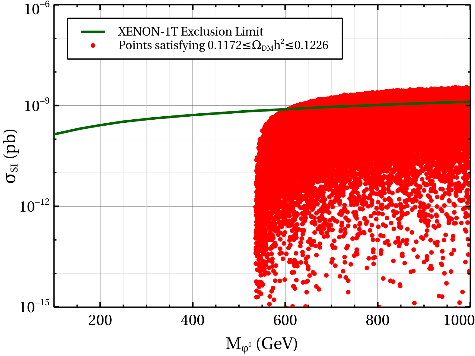
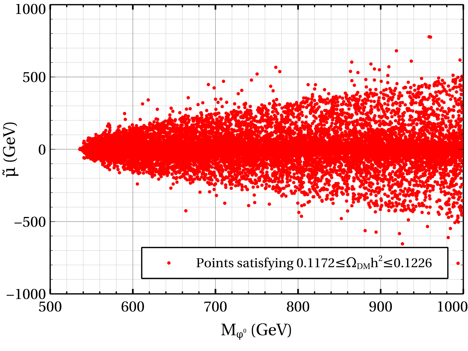
Figure 7: Left panel: Allowed region in $M_{\phi^{0}}-\sigma_{\rm SI}$ plane for the high mass range of $\phi^{0}$, Right panel: Allowed values of trilinear coupling $\tilde{\mu}$, which satisfy Planck relic density bound.

Instead of low mass region of $\phi^{0}$, let us now concentrate on the high mass region. Therefore, in the left panel of Fig. 7 we show the variation $\sigma_{\rm SI}$ with $M_{\phi^{0}}$ for the high mass region. Analogous to the previous case, here also all the red coloured points in $M_{\phi^{0}}-\sigma_{\rm SI}$ plane satisfy the Plank limit of relic density while green solid line represents the current exclusion limit on $\sigma_{\rm SI}$ from the XENON 1T collaboration. From this plot it is evidently seen that the high mass region starts from $M_{\phi^{0}}\simeq 535$ GeV. Therefore, in the present model we have not found any parameter space for the dark matter mass lies between $\sim 90$ GeV to $\sim 534$ GeV. A possible reason is that in this intermediated mass region the main dark matter annihilation channels are $\phi^{0}\phi^{0}\rightarrow W^{+}W^{-}\,,ZZ$ and the annihilation cross sections for these processes are too high to maintain relic abundance in the right ballpark. On the other hand, in the higher mass region, one can only satisfy the Planck bound for low values of $\tilde{\mu}$ i.e. $|\tilde{\mu}|\mathrel{\mathchoice{\vbox{\offinterlineskip\halign{\hfil$\displaystyle#$\hfil\cr<\cr\sim\cr}}}{\vbox{\offinterlineskip\halign{\hfil$\textstyle#$\hfil\cr<\cr\sim\cr}}}{\vbox{\offinterlineskip\halign{\hfil$\scriptstyle#$\hfil\cr<\cr\sim\cr}}}{\vbox{\offinterlineskip\halign{\hfil$\scriptscriptstyle#$\hfil\cr<\cr\sim\cr}}}}500$ GeV (see plot in the right panel of Fig. 7). Otherwise, $\phi^{0}$ will dominantly self annihilate to the components of scalar triplet $\Delta$, which will jeopardise the viability $\phi^{0}$ as a DM candidate by reducing its relic density severely. Therefore, one has to lower the value of $\tilde{\mu}$ by properly adjusting the parameters $\Delta M_{\pm}$ and $\lambda$’s (mainly $\lambda_{6}$ and $\lambda_{9}$), which critically constrain $\Delta M_{\pm}=\sqrt{M^{2}_{\phi^{\pm}}-M^{2}_{\phi^{0}}}$ within a very small range. As a result for the low value of $\tilde{\mu}$ ($\Delta M^{2}_{\pm}$), similar to the intermediate mass range of $M_{\phi^{0}}$ ($90\text{ GeV}\leq M_{\phi^{0}}\leq 534$ GeV), the annihilation channels $W^{+}W^{-}$ and $ZZ$ again become the dominant processes in the higher mass region as well. However, in this case low value of $\Delta M^{2}_{\pm}$ induces significant self annihilation as well as co-annihilation among the odd sector particles which substantially increase the relic density $\Omega h^{2}$ so that it satisfies the Plank limit.

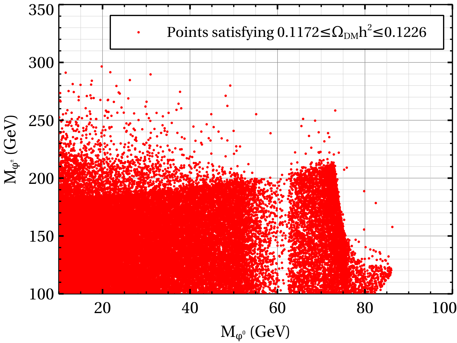
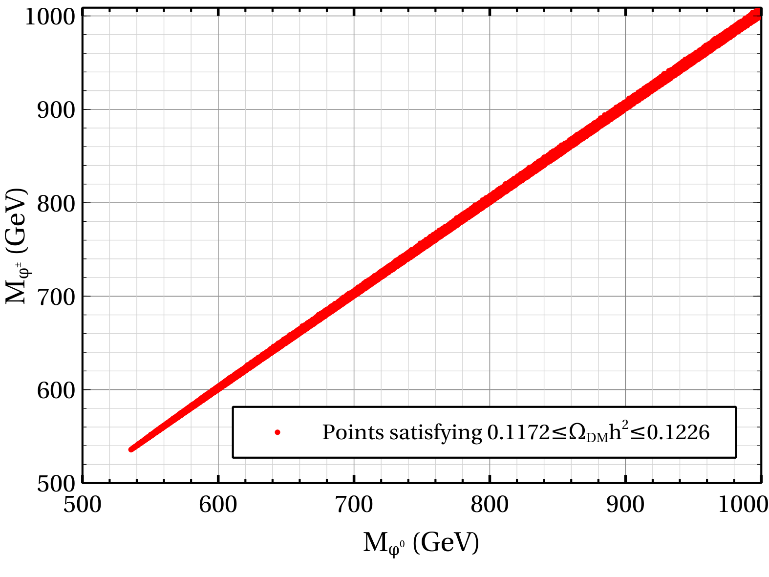
Figure 8: Allowed values of inert charged scalar mass with respect to the mass of $\phi^{0}$ for low mass region (left panel) and high mass region (right panel).

The effect of co-annihilation can be clearly understood by comparing plots in both the panels of Fig. 8. The left panel shows the allowed values of $\phi^{\pm}$ which satisfy the relic density for the low mass region of $\phi^{0}$. It is seen that for a particular value of $M_{\phi^{0}}$, mass of $\phi^{\pm}$ can vary between its lowest possible value of 100 GeV to $\sim 250$ GeV and for such a large mass difference between $\phi^{0}$ and $\phi^{\pm}$ there is practically no effect of co-annihilation. On the other hand, the right panel of Fig. 8 clearly depicts that to satisfy the Planck limit on dark matter relic density, one needs very small mass difference between LOP and $\phi^{\pm}$, which evidently illustrate the effect of co-annihilation on $\Omega h^{2}$ in the high mass region of $\phi^{0}$.

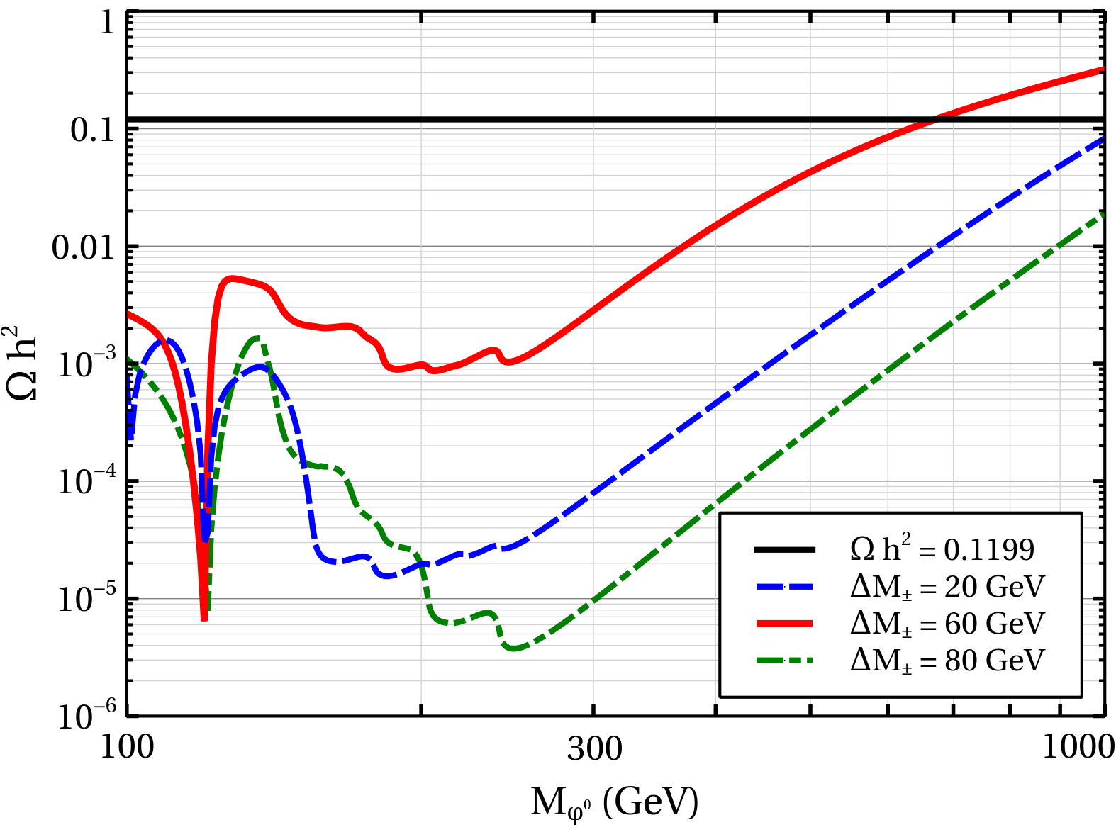
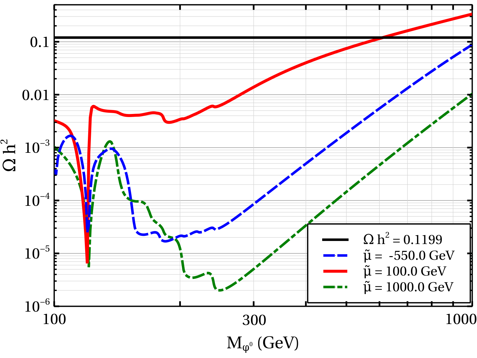
Figure 9: Variation of dark matter relic density with the mass of $\phi^{0}$ for three different values of $\Delta M_{\pm}$ (left panel) and $\tilde{\mu}$ (right panel).

Now, to understand the effects of the trilinear scalar coupling $\tilde{\mu}$ and mass splitting $\Delta M_{\pm}$ on the dark matter relic density we have plotted the variation $\Omega h^{2}$ with $M_{\phi^{0}}$ for three different values of $\tilde{\mu}$ and $\Delta M_{\pm}$ respectively in Fig. 9. In the left panel, three different coloured lines in $M_{\phi^{0}}-\Omega h^{2}$ plane represent three differently chosen values of $\Delta M_{\pm}$ i.e. $\Delta M_{\pm}=20$ GeV (blue dashed line), 60 GeV (red solid line) and 80 GeV (green dashed dot line). This figure has been generated for $M_{H^{\pm\pm}}=156.90$ GeV, $M_{H^{\pm}}=203.39$ GeV, $M_{H^{0}}=M_{A^{0}}=241.03$ GeV, $\lambda_{\Phi}=0.0203$, $\lambda_{5}=0.02$, $\lambda_{6}=-0.1\times 10^{-1}$, $\lambda_{7}=0.41\times 10^{-3}$, $\lambda_{8}=0.1\times 10^{-1}$, $\lambda_{9}=0.41\times 10^{-1}$ and $v_{t}=3$ GeV. From this plot it appears that for the above mentioned set of model parameters there is a unique value of $\Delta M_{\pm}=60$ GeV for which dark matter relic density satisfies Planck limit when $M_{\phi^{0}}=671$ GeV. In this particular situation, $\Delta M_{\pm}=60$ GeV corresponds to a mass difference of $2.677$ GeV between $\phi^{\pm}$ and LOP ($\phi^{0}$) while the mass of CP odd inert scalar $a^{0}$ is 675.896 GeV. In this case, the annihilation and co-annihilation channels which have dominant contributions to the dark matter relic density are $\phi^{0}\phi^{0}\rightarrow W^{+}W^{-},\,ZZ$, $\phi^{0}\phi^{+}\rightarrow W^{+}\gamma,\,W^{+}Z$, $\phi^{+}\phi^{-}\rightarrow W^{+}W^{-},\,\gamma\gamma,\,Z\gamma,\,H^{++}H^{--}$, $a^{0}a^{0}\rightarrow W^{+}W^{-},\,ZZ$, $\phi^{+}a^{0}\rightarrow W^{+}\gamma$. Now if we fix the mass of LOP to a particular value then one can not reproduce the observed relic density by lowering the mass gap between $\phi^{0}$ and $\phi^{\pm}$ arbitrarily small. This can well be understood if we see the expression of trilinear scalar coupling between the triplet $\Delta$ and inert doublet $\Phi$ given in Eq. 94. From this equation, one can notice that for a particular chosen values of $\lambda_{6}$, $\lambda_{8}$, $\lambda_{9}$ and $M_{\phi^{0}}$ there exists a definite range of $\Delta M_{\pm}$ for which the absolute value of $\tilde{\mu}$ lies within the limit specified by the plot in the right panel of Fig. 7. The value of $\Delta M_{\pm}$ beyond this range will enhance the absolute value of $\tilde{\mu}$, which will eventually reduce the dark matter relic density by increasing the annihilation cross section. This feature has been illustrated in the right panel of Fig. 9, where three adopted values of $\tilde{\mu}$ correspond to $\Delta M_{\pm}=21.21$ GeV (blue dashed line), 56.64 GeV (red solid line) and 83.82 GeV (green dashed dot line). Moreover, for a particular set of model parameters one can easily find the allowed values of $\Delta{M_{\pm}}$ for $535\text{ GeV}\leq M_{\phi^{0}}\leq 1000\text{ GeV}$ by setting $|\tilde{\mu}|\mathrel{\mathchoice{\vbox{\offinterlineskip\halign{\hfil$\displaystyle#$\hfil\cr<\cr\sim\cr}}}{\vbox{\offinterlineskip\halign{\hfil$\textstyle#$\hfil\cr<\cr\sim\cr}}}{\vbox{\offinterlineskip\halign{\hfil$\scriptstyle#$\hfil\cr<\cr\sim\cr}}}{\vbox{\offinterlineskip\halign{\hfil$\scriptscriptstyle#$\hfil\cr<\cr\sim\cr}}}}500$ GeV (from the right panel of Fig. 9). Using this upper limit on the absolute value of $\tilde{\mu}$, we find a range of allowed values of $\Delta M_{\pm}$ lying between 25.8 GeV to 70.03 GeV which satisfy the Planck limit on relic density for the chosen set of model parameters mention above. Now both panels of Fig. 7 reveal that, this range of $\Delta M_{\pm}$ is indeed true for this set of model parameters as in both panels the blue and green lines do not satisfy the Planck limit since the parameter $\Delta M_{\pm}$ corresponding to these lines lie outside the above specified range.

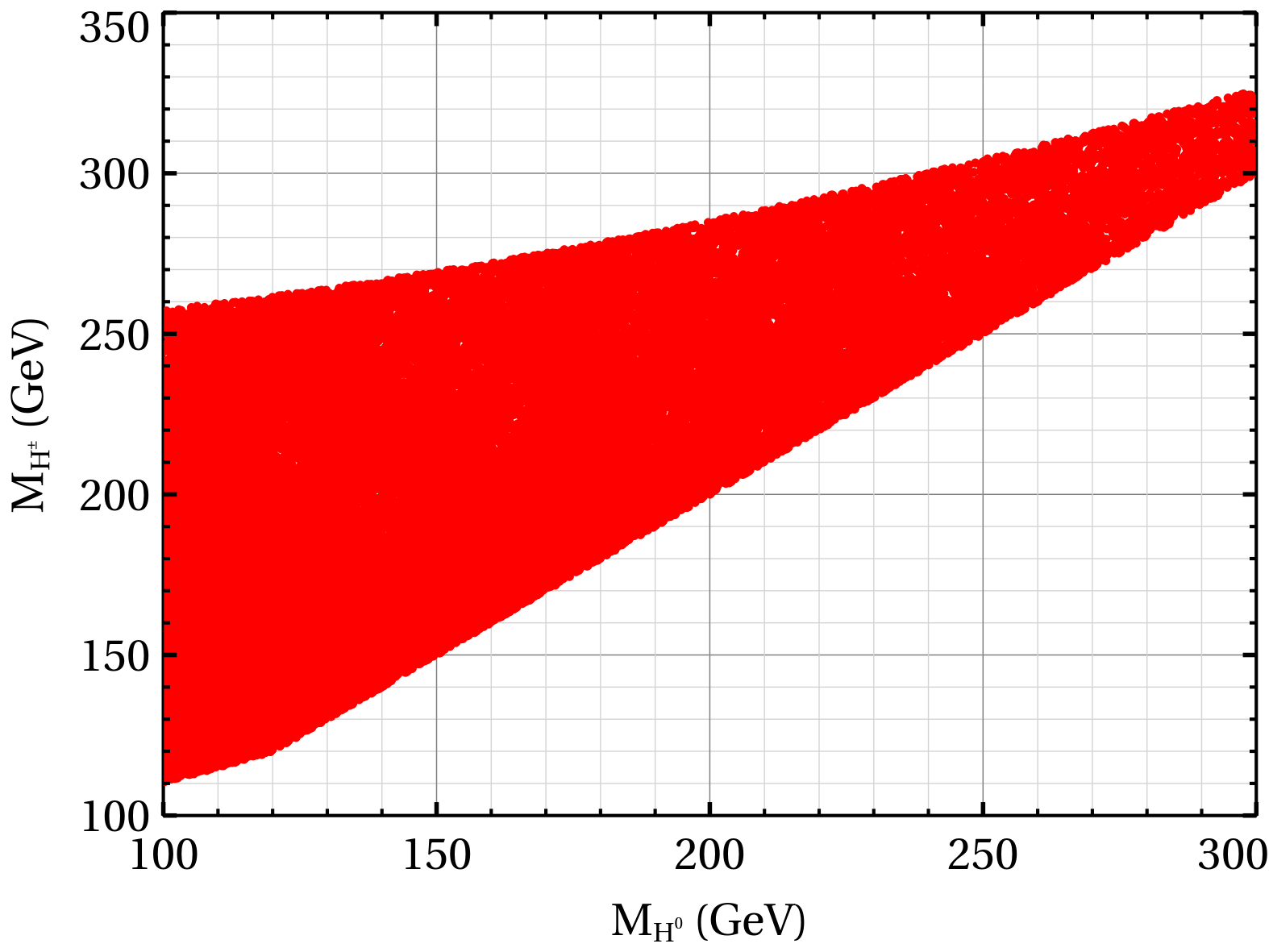
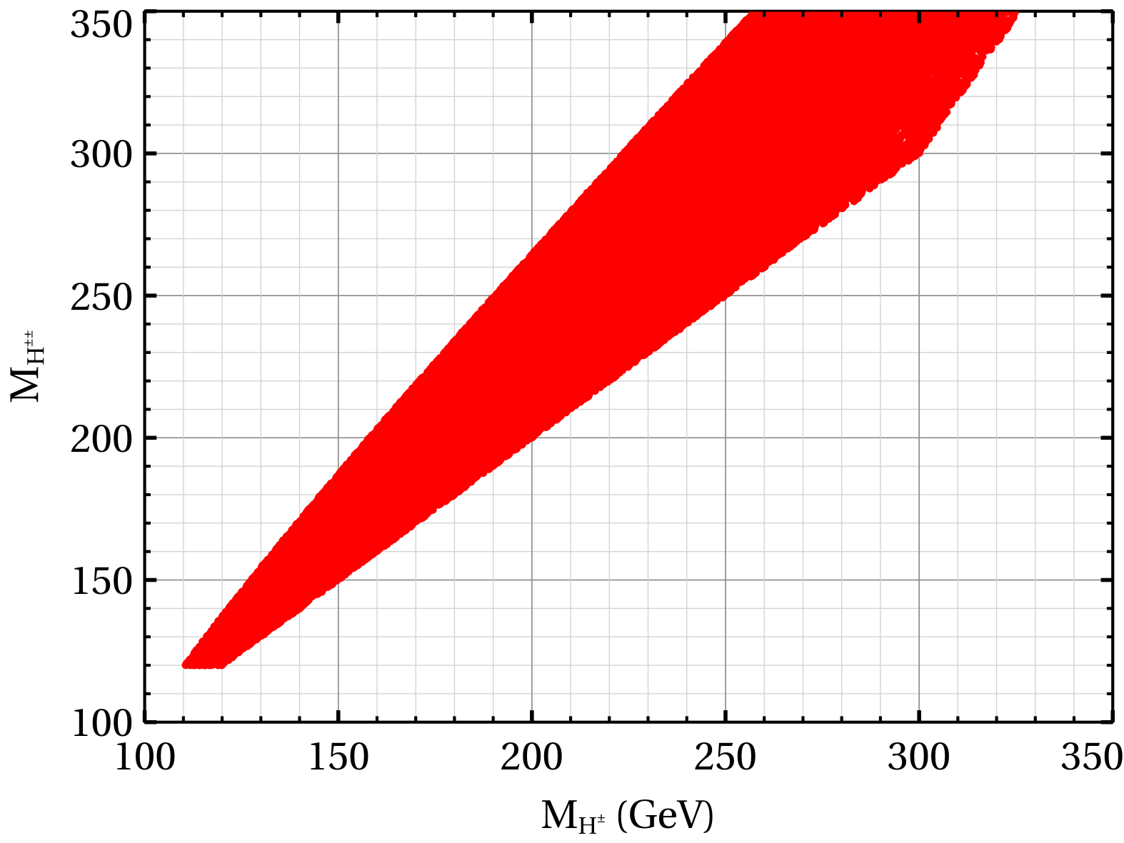
Figure 10: Allowed mass ranges for the BSM scalars, which satisfy all the theoretical and experimental constrains considered in this work.

Next, in the both panels of Fig. 10 we demonstrate the allowed mass ranges of the components of triplet scalar $\Delta$, which satisfy all the theoretical constrains such as unitarity, vacuum stability etc. and the relevant experimental bounds mainly from LEP, LHC etc. In the left panel, we have presented the allowed ranges of $M_{H^{0}}$ and $M_{H^{\pm}}$ while the region allowed in $M_{H^{0}}-M_{H^{\pm\pm}}$ plane has been shown in the right panel. We have checked that these allowed mass ranges of BSM scalars also satisfy the dark matter relic density (in both the allowed regions) and the experimental upper bound obtain from the non-observation of flavour violating decay like $\mu\rightarrow e\,\gamma$ (see Eq. 77 and related discussions in Section III). Note that the nature of these two plots (aligned around a line with slope $45^{\circ}$) mainly arise due to the unitarity constrains discussed in Section II.1.2.

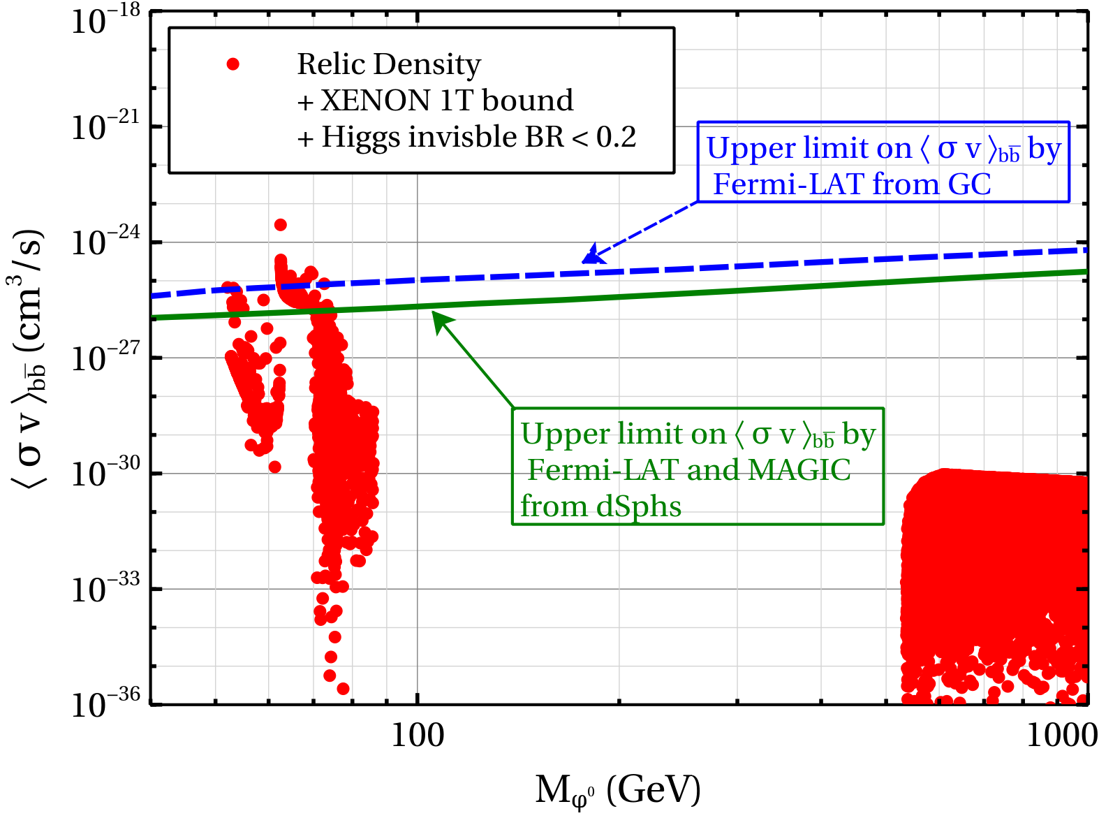
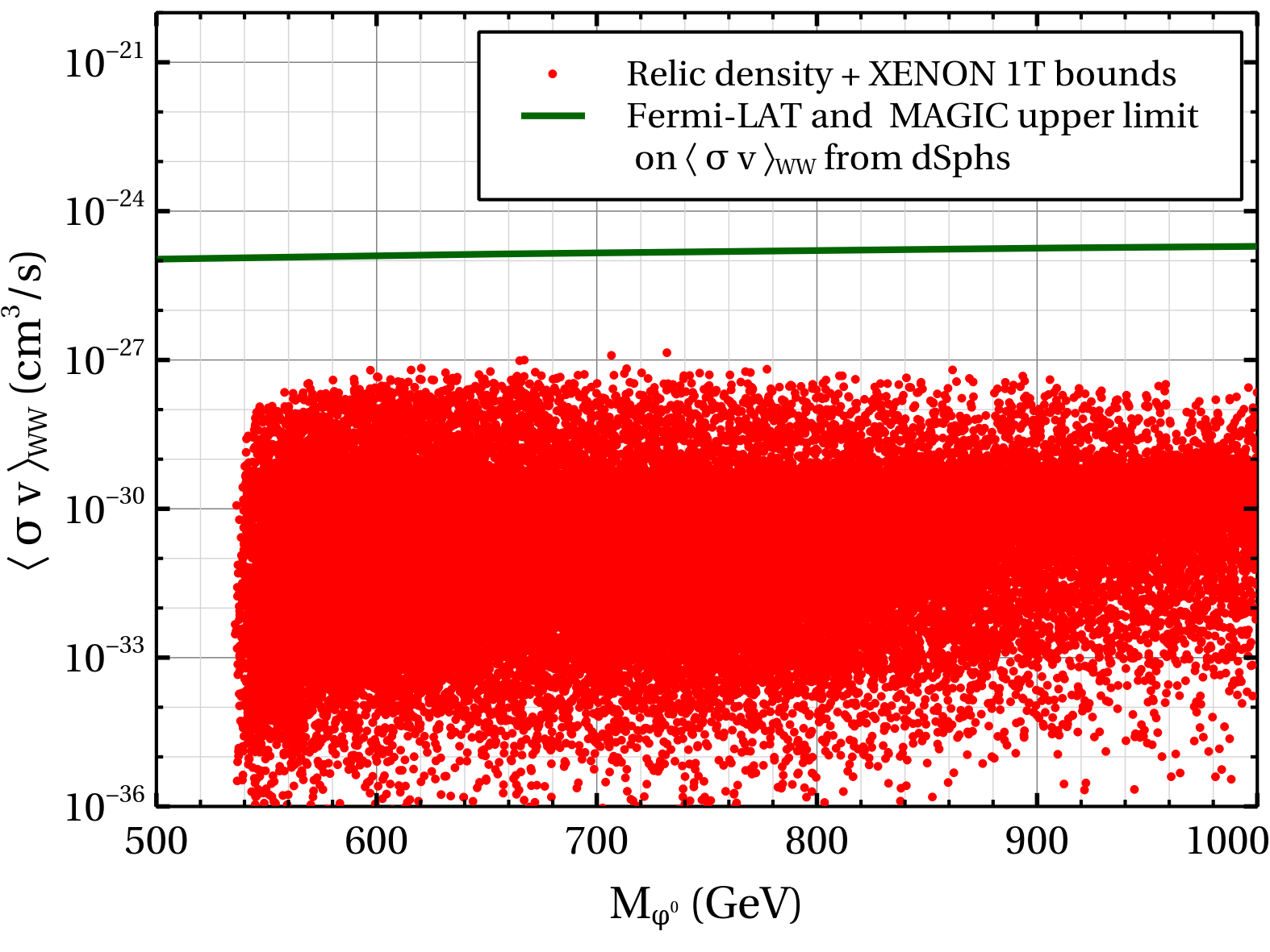
Figure 11: Annihilation cross sections of $\phi^{0}$ at the present epoch for $b\bar{b}$ (left panel) and $W^{+}W^{-}$ (right panel) final states.

Finally, we have computed the annihilation cross section of LOP ($\phi^{0}$) at the present epoch for $b\bar{b}$ and $W^{+}W^{-}$ final states and these are plotted in the left and right panels of Fig. 11 respectively. In each panel, annihilation cross section for a particular channel is computed for the model parameter space which has satisfied all the theoretical and experimental constraints i.e. unitarity, vacuum stability, Planck limit on relic density, bounds on $\sigma_{\rm SI}$ from the XENON 1T collaboration, constrains on the invisible decay width and signal strength of $h^{0}$ from LHC etc. The dark matter annihilation cross sections computed in the present model for two different final states are compared with the existing observational bounds on the same quantities. The non-observation of any significant gamma-ray excess from the dwarf spheroidal galaxies (dSphs) has put an upper limit on the dark matter annihilation cross sections for various final states. Recently a joint analysis 1601.06590 by the Fermi-LAT and the MAGIC collaborations have provided upper limits on dark matter annihilation cross section for different final states like $b\bar{b}$, $W^{+}W^{-}$, $\mu^{+}\mu^{-}$, $\tau^{+}\tau^{-}$ from the observations of 15 dSphs by the Fermi-LAT for 6 years and also 158 hours of observation of Segue 1 satellite galaxy by the MAGIC collaboration. These upper limits on a specific final state are indicated in each panel by a green solid line. On the other hand, a more recent analysis by the Fermi-LAT collaboration 1704.03910 on the Galactic centre gamma-ray excess (GCE) disfavours the dark matter interpretation of this long standing puzzle as they have also found gamma-ray excess from a region where the dark matter signal is not expected i.e. along the Galactic plane. Thus considering a different astrophysical origin of this gamma-ray excess (other than dark matter), they have also reported upper limits on the dark matter annihilation cross sections for $b\bar{b}$ and $\tau^{+}\tau^{-}$ channels. In the left panel, for comparison, we have also plotted the upper limits on $b\bar{b}$ final state (blue dashed line) from the GCE. From the left panel of Fig. 11, it appears that some portions of the allowed parameter space are already ruled by these indirect observations. However, in the high mass region for both $b\bar{b}$ and $W^{+}W^{-}$ final states the limits from indirect detection are not as strong as in the low mass region.

V Collider signature of dark matter at the 13 TeV LHC

In this section we perform dark matter searches in a qualitative way at the LHC of centre of momentum energy ($\sqrt{s}$) 13 TeV. Since the dark matter particles are invisible, therefore they reveal their presence only as missing transverse energy ($E_{T}/\;\>\,\,$). Furthermore, the inert sector is odd under $\mathbb{Z}_{2}$ symmetry, consequently the inert scalars are produced in pairs e.g. $\phi^{+}\phi^{-}$, $\phi^{0}a^{0}$, $\phi^{\pm}a^{0}$, $\phi^{\pm}\phi^{0}$ and $a^{0}a^{0}$, where $\phi^{0}$ is the stable cold dark matter candidate. For the purpose of collider study we set the triplet VEV $v_{t}$ at 3 GeV. In the following, we consider some benchmark points (given in Table 1) which we have chosen from the parameter space permitted by the all constraints including dark matter relic abundance and direct detection data. Further, it is evident from the earlier discussions given in the introduction that the masses of the non-standard scalars of the chosen benchmark points also satisfy the present collider bounds obtained from the LHC data. Moreover, with these given benchmark points we are trying to show the variation of significance of dark matter search at the future LHC experiments. For the selected benchmark points $\phi^{\pm}$ and $a^{0}$ decay into $W^{\pm}\phi^{0}$ and $Z\phi^{0}$ respectively with 100% branching ratio. Based on the decay channels of $W^{\pm}$, $Z$, several final states (e.g. ${\rm jets}+E_{T}/\;\>$, ${\rm leptons}+E_{T}/\;\>$, ${\rm jets}+{\rm leptons}+E_{T}/\;\>$) can be observed at future LHC experiments.

Benchmark Points

$\tan{\alpha}$

$M_{H^{\pm\pm}}$

$M_{H^{\pm}}$

$M_{H^{0}}(=M_{A^{0}})$

$M_{\phi^{0}}$

$M_{\phi^{\pm}}$

$M_{a^{0}}$

$\lambda_{\Phi}$

$\lambda_{5}$

$\lambda_{6}$

$\lambda_{7}$

$\lambda_{8}$

$\lambda_{9}$

$\Omega h^{2}$

$\sigma_{\rm SI}$

$(\rm GeV)$

$(\rm GeV)$

$(\rm GeV)$

$(\rm GeV)$

$(\rm GeV)$

$(\rm GeV)$

($pb$)

BP1

$-1.6\times 10^{-5}$

130.96

196.05

244.42

56.08

151.73

207.54

$0.15\times 10^{-2}$

$-0.23\times 10^{-3}$

$0.28\times 10^{-2}$

0.43

$0.55\times 10^{-1}$

$0.28\times 10^{-3}$

0.1212

$3.46\times 10^{-11}$

BP2

$2.1\times 10^{-3}$

161.82

191.16

216.65

52.24

157.90

222.83

$0.12\times 10^{-3}$

$-0.16\times 10^{-3}$

$0.42\times 10^{-1}$

-0.20

$-0.54\times 10^{-1}$

$-0.60\times 10^{-4}$

0.1217

$2.65\times 10^{-11}$

BP3

$2.0\times 10^{-6}$

187.07

204.95

221.34

74.00

178.00

240.62

$0.14$

$0.86\times 10^{-3}$

$0.70\times 10^{-4}$

$0.40\times 10^{-4}$

$0.17$

$-0.14\times 10^{-2}$

0.1177

$6.01\times 10^{-12}$

Table 1: Benchmark points for dark matter searches at the LHC with corresponding dark matter relic density and direct detection cross section.

On the basis of best possible decay modes and production cross sections we have selected the following processes (Eq. 109a-109d). After that depending on the significance we have studied some final states at the LHC. At this point we would like to mention that due to the mixing of the triplet scalar fields with the SM doublet fields, in each of the following processes there are extra contributions coming from $\mathbb{Z}_{2}$ even non-standard scalars which are absent in typical Inert Doublet Model (IDM). However, their contributions have no practical significance in the processes.

$$a)\leavevmode\nobreak\ p\leavevmode\nobreak\ p \rightarrow \phi^{+}\phi^{-}\rightarrow W^{+}\phi^{0}+W^{-}\phi^{0}\equiv W^{+}W^{-}E_{T}/\;\>\,,$$ (109a)

$$b)\leavevmode\nobreak\ p\leavevmode\nobreak\ p \rightarrow \phi^{0}a^{0}\rightarrow Z\phi^{0}\phi^{0}\equiv ZE_{T}/\;\>\,,$$ (109b)

$$c)\leavevmode\nobreak\ p\leavevmode\nobreak\ p \rightarrow \phi^{\pm}a^{0}\rightarrow W^{\pm}Z\phi^{0}\phi^{0}\equiv W^{\pm}ZE_{T}/\;\>\,,$$ (109c)

$$d)\leavevmode\nobreak\ p\leavevmode\nobreak\ p \rightarrow \phi^{\pm}\phi^{0}\rightarrow W^{\pm}\phi^{0}\phi^{0}\equiv W^{\pm}E_{T}/\;\>\,.$$ (109d)

In Table. 2 we have alluded the gross production cross sections at 13 TeV LHC for different processes (given in above) for the chosen benchmark points. Note that the values of cross sections for the signal events have been calculated at leading order (LO) therefore in this sense our choice is conservative as the $K$-factors for the next to leading order (NLO) corrections are larger than unity.

Benchmark Points	process (a) ($pb$)	process (b) ($pb$)	process (c) ($pb$)	process (d) ($pb$)
BP1	0.04333	0.05861	0.04009	0.2756
BP2	0.03738	0.04787	0.03204	0.2570
BP3	0.02390	0.03105	0.02236	0.1394

Table 2: LO cross sections (in $pb$) for the processes given in Eq. 109a-109d at $\sqrt{s}=13$ TeV.

In our analysis, we use FeynRules Alloul:2013bka from which we have produced UFO model files required in Madgraph5 Alwall:2014hca to generate the signal events at the LO parton level. For the purpose of SM background processes, we have generated events using Madgraph5. To simulate showering and hadronisation effects, we have passed the unweighted parton level through the Pythia(v6.4) Sjostrand:2006za , including fragmentation. We have done the detector simulation using the Delphes(v3) deFavereau:2013fsa . Jets are constructed using Fastjet Cacciari:2011ma with anti-$k_{T}$ Cacciari:2008gp jet clustering algorithm with proper MLM matching scheme chosen for background processes. The production cross sections are calculated using the NNPDF3.0 parton distributions. Finally, we perform the cut analyses using MadAnalysis5 Conte:2012fm .

Before we proceed to simulate the events we should impose some basic cuts as our final states under consideration may also result from hard subprocesses associated with initial and final state radiation, or soft decays. Hence, we demand that

$$\Delta R_{jj}>0.4,\leavevmode\nobreak\ \leavevmode\nobreak\ \leavevmode\nobreak\ \leavevmode\nobreak\ \Delta R_{\ell\ell}>0.7,\leavevmode\nobreak\ \leavevmode\nobreak\ \leavevmode\nobreak\ \leavevmode\nobreak\ \Delta R_{j\ell}>0.7,$$ (110a)

$$\Delta R_{bj}>0.7,\leavevmode\nobreak\ \leavevmode\nobreak\ \leavevmode\nobreak\ \leavevmode\nobreak\ \Delta R_{b\ell}>0.2,$$ (110b)

$$p_{T}^{j}>20\leavevmode\nobreak\ {\rm GeV},\leavevmode\nobreak\ \leavevmode\nobreak\ \leavevmode\nobreak\ \leavevmode\nobreak\ |\eta_{j}|<2.5,$$ (110c)

$$p_{T}^{\ell}>10\leavevmode\nobreak\ {\rm GeV},\leavevmode\nobreak\ \leavevmode\nobreak\ \leavevmode\nobreak\ \leavevmode\nobreak\ |\eta_{\ell}|<2.5,$$ (110d)

$$p_{T}^{\gamma}>10\leavevmode\nobreak\ {\rm GeV},\leavevmode\nobreak\ \leavevmode\nobreak\ \leavevmode\nobreak\ \leavevmode\nobreak\ |\eta_{\gamma}|<2.5.$$ (110e)

Moreover, we consider the following $p_{T}$-dependent $b$-tagging efficiency given by the ATLAS collaboration ATLAS:2014pla ,

$$\epsilon_{b}=\begin{cases}0&p_{T}^{b}\leq 30\leavevmode\nobreak\ \rm GeV\;,\\ 0.6&30\leavevmode\nobreak\ {\rm GeV}<p_{T}^{b}<50\leavevmode\nobreak\ {\rm GeV}\;,\\ 0.75&50\leavevmode\nobreak\ {\rm GeV}<p_{T}^{b}<400\leavevmode\nobreak\ {\rm GeV}\;,\\ 0.5&p_{T}^{b}>400\leavevmode\nobreak\ \rm GeV\;.\end{cases}$$ (111)

Apart from this, we also introduce a mistagging probability of 10% (1%) for charm-jets (light-quark and gluon jets). Further, the absolute rapidity of $b$-jets are demanded to be less than 2.5 $(|\eta_{b}|<2.5)$.

V.1 Cut Analysis:

All processes given in Eq. 109a-109d may contribute to several final states which we are going to study in this work. These final sates can be tagged as $Signal$ while the SM processes which mimic the signal are considered as $Background$. In order to improve the signal to background ratio we will impose some selection cuts in addition to the basic cuts given in Eq. 110. After imposing the selection cuts, if there exists $N_{S}$ and $N_{B}$ number of events for signal and background respectively, then we can calculate the significance ($S$) of any particular final states using the following relation

$$S = \frac{N_{S}}{\sqrt{N_{S}+N_{B}}}\,\ .$$ (112)

Now we are in a position where we can study some final states which arise from four sub-processes given in Eq. 109a-109d,

$$(i) 2\ell+E_{T}/\;\>\,,$$ (113a)

$$(ii) 2j+E_{T}/\;\>\,,$$ (113b)

$$(iii) 3\ell+E_{T}/\;\>\,,$$ (113c)

where $\ell\equiv e,\mu$ and $j$ represents ordinary light jets. For the practical purpose we need to consider the following SM subprocesses as backgrounds to the aforementioned final states.

• $W^{\pm}+\rm jets$: We consider this process with up to two hard jets as this process serves as the dominant background for the signal which contains hard $E_{T}/\;\>$ in the final state and ordinary light jets.

• $Z+\rm jets$: This can be considered as significant background for the signal with two charged leptons in the final state. In this case also we consider two hard jets for semi-inclusive cross section.

• $VV+\rm jets$ (where $V=W^{\pm},Z$): We have estimated the processes with two hard jets because they exactly mimic some of the gross production channels.

• $t\bar{t}(+\rm jets)$: $t\bar{t}$ production with two additional hard jets, can play as one of the major dominant background for some of the three final states.

• Single top + jets: This will contribute mainly to final state $(ii)$.

• $t\bar{t}+(W^{\pm}/Z/\gamma)$: Analogous to $t\bar{t}(+\rm jets)$, these processes could also contribute to the total SM background, but with much smaller production cross sections.

• $VVV$ (where $V=W^{\pm},Z$): In the case of leptonic decays of $W^{\pm},Z$ we could consider this process in the SM background.

• QCD($\leq 3$ jets): Pure QCD processes play as the most dominant SM-background for hadronic final states such as multi-jet production where $E_{T}/\;\>$ comes either from the jets fragmenting into neutrinos or simply from the mismeasurement of the jet energy.

(i) ${\underline{2\ell+E_{T}/\;\>}}$  : This final state can be produced from the processes (109a), (109b) and (109c). In this final state we have two charged leptons with $E_{T}/\;\>$. Therefore, this signal is relatively clean however production cross section is small. Here in the background events, the $E_{T}/\;\>$  comes only from the neutrinos, while for the signal events, it arises from $\phi^{0}$. The mass difference between $\phi^{0}$ and the decaying $a^{0}$ significantly enhances the $E_{T}/\;\>$. Therefore, by choosing $E_{T}/\;\>>100$ GeV we may inhibit the background and consequently improve the signal significance. Below we mention the selection criteria for this signal.

Cuts Name	Selection Criteria
C1-1	Reject number of $b$-tagged jets with $p_{T}(b)>20$ GeV
C1-2	Select lepton with $p_{T}(\ell_{2})>10$ GeV
C1-3	Reject lepton with $p_{T}(\ell_{3})>10$ GeV
C1-4	Select $\Delta R(\ell_{i}\ell_{j})<$ 2.8
C1-5	Reject additional jet with $p_{T}(j_{1})>20$ GeV
C1-6	Select $E_{T}/\;\>>100$ GeV

Table 3: Required selection cuts for $2\ell+E_{T}/\;\>$ final state.

With the above mentioned criteria, we have obtained the following significance for this signal for the chosen benchmark points.

Benchmark Points	process (a) ($fb$)	process (b) ($fb$)	process (c) ($fb$)	Total ($fb$)	Significance ($S$)
BP1	0.0618	0.3516	0.0307	0.4441	3.72
BP2	0.0537	0.3128	0.0264	0.3929	3.29
BP3	0.0388	0.2192	0.0201	0.2781	2.33

Table 4: After imposing all cuts the cross sections (in $fb$) for the processes given in Eq. 109a-109d which are contributed in this signal at $\sqrt{s}=13$ TeV. Also the corresponding statistical significances for an integrated luminosity of 3000 $fb^{-1}$ are given for all benchmark points. The total background cross section for this signal after all cuts is 42.33 $fb$.

After passing the signal and background events through the selection criteria (given in Table  3) we estimate the corresponding significance reach at the highest plausible integrated luminosity that can be achieved at the LHC. It can be seen from this Table 4, the maximum significance greater than $3.5\sigma$ is attained for the BP1, due to the largest production cross section. The signal significance is small for the benchmark BP3. This analysis shows that there will be a finite chances to search dark matter via this signal at the future LHC running at 13 TeV of integrated luminosity 3000$fb^{-1}$.

(ii) ${\underline{2j+E_{T}/\;\>}}$  : This final state comes from the processes (109b), (109c) and (109d). The same signal has been studied in the context of IDM in Poulose:2016lvz at the 13 TeV LHC. As far as the cross section is concerned, this final state possesses larger value with respect to other final states. However pure QCD process with large cross section which we have considered in the SM background suppress the significance. Nevertheless, in the following we are trying to probe the signal by imposing some judicious criteria which may improve the signal efficiencies with respect to the SM background.

Cuts Name	Selection Criteria
C2-1	Reject number of $b$-tagged jets with $p_{T}(b)>20$ GeV
C2-2	Select $2^{nd}$ jet with $p_{T}(j_{2})>30$ GeV
C2-3	Reject $3^{rd}$ jet with $p_{T}(j_{3})>20$ GeV
C2-4	Reject $1^{st}$ lepton with $p_{T}(\ell_{1})>10$ GeV
C2-5	Select $E_{T}/\;\>>110$ GeV

Table 5: Required selection cuts for $2j+E_{T}/\;\>$ final state.

These criteria (given in Table 5) ensure that in the signal we have two leading jets with $p_{T}(j)$ greater than 30 GeV. Fourth cut ensures that we have no leptons in our signal. Also the selection of $E_{T}/\;\>$  greater than 110 GeV helps us to reduce the dominant backgrounds along with pure QCD background significantly. Below we have given the statistics for the signal for the selected benchmark points with respect to SM backgrounds. Specifically we have given (in Table 6) the cross sections for the individual channel after the selection cuts for the selected benchmark points and also the corresponding significances. For the first two benchmark points we can have the significance up to $\gtrsim 1.4\sigma$ but require high luminosity 3000 $fb^{-1}$. So it is hard to probe this model via this signal at the LHC even with very high luminosity.

Benchmark Points	process (b) ($fb$)	process (c) ($fb$)	process (d) ($fb$)	Total ($fb$)	Significance ($S$)
BP1	4.204	1.392	13.464	19.06	1.49
BP2	3.786	1.271	12.824	17.88	1.40
BP3	2.637	0.885	8.206	11.73	0.92

Table 6: After using all cuts the cross sections (in $fb$) for the processes given in Eq. 109a-109d which are contributed in this signal at $\sqrt{s}=13$ TeV. Also the corresponding statistical significances for an integrated luminosity of 3000 $fb^{-1}$ are given for all benchmark points. The total background cross section for this signal after all cut is 492728.60 $fb$.

(iii) ${\underline{3\ell+E_{T}/\;\>}}$  : Finally we consider this signal which arises from the process (109c) only. In Ref. Datta:2016nfz one can find the multilepton signature of IDM including trilepton +$E_{T}/\;\>$  signal at the 13 TeV LHC. In our present model we are also trying to search dark matter at the LHC via this final state. By considering the all relevant SM-backgrounds we have calculated the significance the for this final state.

In the following (Table 7) we have shown the selection criteria by which we can extract signal with respect to background.

Cuts Name	Selection Criteria
C3-1	Reject number of $b$-tagged jets with $p_{T}(b)>20$ GeV
C3-2	Select $3^{rd}$ lepton with $p_{T}(\ell_{3})>10$ GeV
C3-3	Reject $1^{st}$ lepton with $p_{T}(j_{1})>20$ GeV
C3-4	Select $E_{T}/\;\>>100$ GeV

Table 7: Required selection cuts for ${3\ell+E_{T}/\;\>}$ final state.

As we demand that in our signal we require only three lepton so we have select third leading lepton with $p_{T}({l})>$ 10 GeV. We have also rejected any jet with $p_{T}({j})>$ 20 GeV as the signal does not contain any jet. Finally selection of $E_{T}/\;\>>100$ GeV reduces the background substantially.

Benchmark Points	process (c) ($fb$)	Significance ($S$)
BP1	0.0320	1.09
BP2	0.0313	1.07
BP3	0.0235	0.80

Table 8: After implementing all cuts the cross sections (in $fb$) for the processes given in Eq. 109a-109d which are contributed in this signal at $\sqrt{s}=13$ TeV. Also the corresponding statistical significances for an integrated luminosity of 3000 $fb^{-1}$ are given for all benchmark points. The total background cross section for this signal is 2.54 $fb$.

Finally with the above selection criteria we have significance $\gtrsim 1\sigma$ for the first two benchmark points. Hence in this case also, to find the dark matter at LHC through this signal is less attractive at LHC even for high integrated luminosity 3000 $fb^{-1}$.

Before we conclude, it would be relevant to discuss some issues on a region of parameter space which we have not considered in our collider analysis. In general, one can have the region of parameter space (which satisfies all the theoretical constraints as well as dark matter relic abundance and direct detection data) where $\phi^{\pm}$ and $a^{0}$ decay into $H^{\pm}\phi^{0}$ and $A^{0}\phi^{0}$ respectively, in fact with 100% branching ratio. However, we have not considered this region of parameter space in our collider study. First of all in this region of parameter space, the production cross sections of the $\mathbb{Z}_{2}$ odd scalars at the 13 TeV LHC are lower than that of given in the Table 2 due to phase space suppression. Because, in this case for the above decay modes to become kinematically feasible one requires $M_{\phi^{\pm}}>(M_{H^{\pm}}+M_{\phi^{0}})$ and $M_{a^{0}}>(M_{A^{0}}+M_{\phi^{0}})$. Hence, the masses of $\phi^{\pm}$ and $a^{0}$ are larger with respect to the values of masses given in the Table 1. This will drop the signal efficiency.

Additionally, in this region of parameter space, the non-standard scalars $H^{\pm}$ or $A^{0}$ which are produced from the decay of inert scalars are dominantly decaying to various three body decay modes each of which possesses small branching fraction. Moreover, the remaining two body decay modes of these triplet scalars also acquire very tiny branching fractions. Because in the case of leptonic decay modes, the coupling between singly charged Higgs ($H^{\pm}$) and leptons are suppressed due to the tiny neutrino Yukawa coupling while for the hadronic decay modes the coupling of $H^{\pm}$ with quarks are suppressed by the small mixing angle $\beta^{\prime}$. Therefore, if we consider the two body decay modes of $H^{\pm}$ for any particular final state then we will end up with a very small effective cross section due to small branching fractions. Consequently, the signal significance will be very low even at the very high luminosity future collider experiment.

Further, in the case of three body decay modes one may consider the following process (for our chosen value of $v_{t}$)

$$\leavevmode\nobreak\ p\leavevmode\nobreak\ p\rightarrow\phi^{+}\phi^{-} \rightarrow H^{+}\phi^{0}+H^{-}\phi^{0}$$

$$H^{\pm} \hookrightarrow H^{\pm\pm}q\bar{q^{\prime}}\to W^{\pm}W^{\pm}(W^{\pm}W^{*\pm})+q\bar{q^{\prime}}\;.$$

Now, the $W^{\pm}$ produced from $H^{\pm\pm}$ will further decays to either leptons or jets. Hence, in this situation one can reach a stable final state after several decay steps and for each step there will be a suppression due to small branching fraction. We have already mentioned earlier that in this region of parameter space the production cross sections are small and also the small branching fractions (at each decay step) will further suppress the effective cross section for any particular final state. Consequently, in the case of three body decay modes one has the very small signal significances in comparison to the values what we have obtained from our analysis.

Due to the above mentioned facts we have considered the region of parameter space where the $\mathbb{Z}_{2}$ odd scalars $\phi^{\pm}$ and $a^{0}$ decay into $W^{\pm}\phi^{0}$ and $Z\phi^{0}$ with 100% branching ratio.

VI Conclusions

In order to convey the existence of the non-luminous dark matter of the Universe and the origin of tiny neutrino masses, we have considered an extension of the Type-II seesaw model by adding a $\mathbb{Z}_{2}$ odd doublet $\Phi$. We ensure that the CP even component of $\Phi$ is the WIMP dark matter candidate which is stable due to the $\mathbb{Z}_{2}$ symmetry. On the other hand, Higgs triplet scalar field generates the masses of neutrinos via the Type-II seesaw mechanism. Furthermore, in this framework we have derived the full set of unitarity and vacuum stability conditions which have always been very important if one deals with the scalar sector.

In the Type-II seesaw scenario the triplet VEV is very small ($10^{-9}$ GeV to ${\cal O}(1)$ GeV) by the electroweak precision constraint. Hence, for the purpose of neutrino mass generation we set the value of triplet VEV at $10^{-3}$ GeV. We have alluded the absolute values of neutrino masses allowed by the neutrino oscillation data at 3$\sigma$ range. Then we have shown that the sum of masses of three neutrinos for the normal(inverted) hierarchical scenario is around $\sim$ 0.06 eV to 0.1 eV(0.1 eV to 0.2 eV) which respects the bound from cosmological observations (i.e. $\sum m_{\nu}<0.23$ eV). Furthermore, we have calculated the effective Majorana mass parameter $m_{\beta\beta}$ associated with the neutrinoless double $\beta$ decay process. We have derived the upper limit on the mass of the lightest neutrino $m_{1}(m_{3})$ of normal(inverted) hierarchy by satisfying the combined results of cosmological upper bound and neutrino oscillation data. We have also computed the Dirac CP phase $\delta$ that resides in the first and fourth quadrant for the normal hierarchy while it lies between $90^{\circ}-140^{\circ}$ and $220^{\circ}-270^{\circ}$ for the inverted hierarchical scenario. However, the recent results of T2K experiment are favourable for the values of $\delta$ which lie in the third and fourth quadrant instead of the first two quadrants. Finally, we also evaluated the Jarlskog invariant $J_{CP}$ using the model parameters which satisfy the neutrino oscillation data in $3\sigma$ range. We find that it lies below 0.039 irrespective of the neutrino mass hierarchy.

We have also explored the dark matter phenomenology in a great detail by considering $\phi^{0}$ as a WIMP type dark matter candidate of the present scenario. We have considered all possible annihilation channels while calculating the dark matter relic abundance. One should note that, in our case the dark matter particle satisfies the Planck limit ($0.1172\leq\Omega h^{2}\leq 0.1226$ Ade:2015xua ) of relic density only for two distinct mass ranges of $\phi^{0}$. For example, in the low mass range where $M_{\phi^{0}}$ lies below 90 GeV while in the high mass range $M_{\phi^{0}}$ is larger than 535 GeV. For the low mass region we have done our analysis for two different values of triplet scalar VEV $v_{t}$, e.g., $10^{-3}$ GeV and 3 GeV. When $v_{t}=3$ GeV, we have observed that the dark matter with mass $\mathrel{\mathchoice{\vbox{\offinterlineskip\halign{\hfil$\displaystyle#$\hfil\cr<\cr\sim\cr}}}{\vbox{\offinterlineskip\halign{\hfil$\textstyle#$\hfil\cr<\cr\sim\cr}}}{\vbox{\offinterlineskip\halign{\hfil$\scriptstyle#$\hfil\cr<\cr\sim\cr}}}{\vbox{\offinterlineskip\halign{\hfil$\scriptscriptstyle#$\hfil\cr<\cr\sim\cr}}}}50$ GeV also satisfies the relic density. However, those regions are forbidden if one imposes the constraint of invisible branching ratio of the SM-like Higgs boson $h^{0}$. In the low mass range, the dominant contribution to $\langle\sigma{\rm v}\rangle$ comes from $\phi^{0}\phi^{0}\rightarrow b\bar{b}$ ($W^{+}W^{-}$) channel for $M_{\phi^{0}}\mathrel{\mathchoice{\vbox{\offinterlineskip\halign{\hfil$\displaystyle#$\hfil\cr<\cr\sim\cr}}}{\vbox{\offinterlineskip\halign{\hfil$\textstyle#$\hfil\cr<\cr\sim\cr}}}{\vbox{\offinterlineskip\halign{\hfil$\scriptstyle#$\hfil\cr<\cr\sim\cr}}}{\vbox{\offinterlineskip\halign{\hfil$\scriptscriptstyle#$\hfil\cr<\cr\sim\cr}}}}70$ GeV ($\mathrel{\mathchoice{\vbox{\offinterlineskip\halign{\hfil$\displaystyle#$\hfil\cr>\cr\sim\cr}}}{\vbox{\offinterlineskip\halign{\hfil$\textstyle#$\hfil\cr>\cr\sim\cr}}}{\vbox{\offinterlineskip\halign{\hfil$\scriptstyle#$\hfil\cr>\cr\sim\cr}}}{\vbox{\offinterlineskip\halign{\hfil$\scriptscriptstyle#$\hfil\cr>\cr\sim\cr}}}}70$ GeV). Also in the low mass range the co-annihilations among the inert sector particles have no considerable effect on the dark matter relic density, as we have taken $M_{\phi^{\pm}},M_{a^{0}}>100$ GeV. Furthermore, we would like to mention that, there is a distinct feature of the present scenario, with respect to the conventional Inert Doublet Model. The trilinear coupling ($\tilde{\mu}$) between triplet scalar field and inert doublet plays a crucial role in our dark matter analysis. The parameter $\tilde{\mu}$ effectively proportional to the mass difference between the dark matter and the inert charged scalar. Therefore, depending on the mass gap, $\tilde{\mu}$ controls the dark matter annihilation processes. For example, in the low mass region the absolute values of $\tilde{\mu}$ can vary from 0 to $\sim 10^{4}$ GeV as in this case the mass difference between $\phi^{+}$ and $\phi^{0}$ varies between $\sim(20-270)$ GeV. On the other hand, in the high mass region the mass gaps between the inert scalars are required to be very small as a consequence of the significant contributions of different co-annihilation channels to dark matter relic density. Hence, in this case to satisfy the Plank limit one should vary the relevant model parameters in a fine tune way which in turn controls the trilinear coupling $\tilde{\mu}$ (i.e. $|\tilde{\mu}|\mathrel{\mathchoice{\vbox{\offinterlineskip\halign{\hfil$\displaystyle#$\hfil\cr<\cr\sim\cr}}}{\vbox{\offinterlineskip\halign{\hfil$\textstyle#$\hfil\cr<\cr\sim\cr}}}{\vbox{\offinterlineskip\halign{\hfil$\scriptstyle#$\hfil\cr<\cr\sim\cr}}}{\vbox{\offinterlineskip\halign{\hfil$\scriptscriptstyle#$\hfil\cr<\cr\sim\cr}}}}500$ GeV). Apart from that, we have also evaluated the spin-independent scattering cross section of dark matter off the detector nuclei. Our estimations indicate that a major portion of dark matter parameter space in the low mass region has already been ruled out by the XENON 1T experiment. However, there are still some region left which can be tested by the ongoing and future direct detection experiments. Further, we have also noticed that the high mass region is still comparatively less constrained by the exclusion limits from XENON 1T experiments and this region can be a potential dark matter search region for the future “ton scale” direct detection experiments. On the other hand, we have found the similar results from the perspective of indirect search of dark matter. Here also some portions of the allowed parameter space in the low dark mass region has been excluded by the recent analyses of gamma-ray flux from dwarf spheroidal galaxies and also from the Galactic Centre by the Fermi-LAT and MAGIC collaborations. However, similar to the case of direct search, the limits from the indirect detection are also much more relaxed in the high mass region.

Finally, we have investigated the collider signature of the dark matter in terms of missing transverse energy ( $E_{T}/\;\>$ ) at the 13 TeV LHC. Due to the $\mathbb{Z}_{2}$ symmetry the odd particles are produced in pairs. Furthermore, for our chosen benchmark points, satisfying all theoretical and experimental constraints including dark matter relic density, the heavier odd particles decay into the SM gauge bosons and dark matter. Depending on the production channels and the branching fractions of the odd particles one has several final states which can be probed at the current and the future colliders. In our case, we have analysed three final states namely, $2\ell+E_{T}/\;\>\,,\leavevmode\nobreak\ 2j+E_{T}/\;\>\,$ and $3\ell+E_{T}/\;\>\,,$ at the 13 TeV LHC. For each of the final states we have calculated relevant SM backgrounds. With judicious cut selection, we have evaluated the signal significance for an integrated luminosity 3000$fb^{-1}$. From our simulation study it is clearly evident that for the two benchmark point we can have the significance greater than $3\sigma$ for the final state $2\ell+E_{T}/\;\>\,$. Hence, with this signal there will be a finite chance to search dark matter at the future LHC running at 13 TeV of integrated luminosity 3000$fb^{-1}$.

Acknowledgments Both the authors A.B. and A.S. thank Abhisek Dey for computational help. They are also grateful to Subhadeep Mondal for the useful discussions regarding collider study. One of the authors A.B. would like to acknowledge the cluster computing facility (http://cluster.hri.res.in) of Harish-Chandra Research Institute. A.B. would also like to thank the Department of Atomic Energy (DAE), Govt. of INDIA for financial assistance.

Appendix A The eigenvalue equations which are being solved using numerical technique

$$4\mathbb{X}^{3}-\bigg{(}6\lambda+32\lambda_{2}+24\lambda_{3}+24\lambda_{\Phi}\bigg{)}\mathbb{X}^{2}+\bigg{(}-24\lambda^{2}_{1}+48\lambda\lambda_{2}+36\lambda\lambda_{3}-24\lambda_{1}\lambda_{4}-6\lambda^{2}_{4}-16\lambda^{2}_{5}$$

$$-16\lambda_{5}\lambda_{6}-4\lambda^{2}_{6}-24\lambda^{2}_{7}-24\lambda_{7}\lambda_{8}-6\lambda^{2}_{8}+36\lambda\lambda_{\Phi}+192\lambda_{2}\lambda_{\Phi}+144\lambda_{3}\lambda_{\Phi}\bigg{)}\mathbb{X}$$

$$+\bigg{(}128\lambda_{2}\lambda^{2}_{5}+96\lambda_{3}\lambda^{2}_{5}+128\lambda_{2}\lambda_{5}\lambda_{6}+96\lambda_{3}\lambda_{5}\lambda_{6}+32\lambda_{2}\lambda^{2}_{6}+24\lambda_{3}\lambda^{2}_{6}-96\lambda_{1}\lambda_{5}\lambda_{7}-48\lambda_{4}\lambda_{5}\lambda_{7}$$

$$-48\lambda_{1}\lambda_{6}\lambda_{7}-24\lambda_{4}\lambda_{6}\lambda_{7}+36\lambda\lambda^{2}_{7}-48\lambda_{1}\lambda_{5}\lambda_{8}-24\lambda_{4}\lambda_{5}\lambda_{8}-24\lambda_{1}\lambda_{6}\lambda_{8}-12\lambda_{4}\lambda_{6}\lambda_{8}+36\lambda\lambda_{7}\lambda_{8}$$

$$+9\lambda\lambda^{2}_{8}+144\lambda^{2}_{1}\lambda_{\Phi}-288\lambda\lambda_{2}\lambda_{\Phi}-216\lambda\lambda_{3}\lambda_{\Phi}+144\lambda_{1}\lambda_{4}\lambda_{\Phi}+36\lambda^{2}_{4}\lambda_{\Phi}\bigg{)}=0.$$ (A-1)

$$2\mathbb{X}^{3}-\bigg{(}\lambda+4\lambda_{2}+8\lambda_{3}+4\lambda_{\Phi}\bigg{)}\mathbb{X}^{2}+\bigg{(}2\lambda\lambda_{2}+4\lambda\lambda_{3}-2\lambda^{2}_{4}-2\lambda^{2}_{6}-2\lambda^{2}_{8}+2\lambda\lambda_{\Phi}+8\lambda_{2}\lambda_{\Phi}$$

$$+16\lambda_{3}\lambda_{\Phi}\bigg{)}\mathbb{X}+\bigg{(}4\lambda_{2}\lambda^{2}_{6}+8\lambda_{3}\lambda^{2}_{6}-4\lambda_{4}\lambda_{6}\lambda_{8}+\lambda\lambda^{2}_{8}-4\lambda\lambda_{2}\lambda_{\Phi}-8\lambda\lambda_{3}\lambda_{\Phi}+4\lambda^{2}_{4}\lambda_{\Phi}\bigg{)}=0.$$ (A-2)

By solving the above cubic Eqs. A-1 and A-2 using numerical technique we have obtained the eigenvalues of $\mathcal{M}_{2}$. Whereas, from the Eq. A-2 we have evaluated the eigenvalues of $\mathcal{M}_{4}$ using the same numerical technique.

Appendix B Explicit form of BFB conditions

$$\lambda\geq 0,\leavevmode\nobreak\ \leavevmode\nobreak\ \lambda_{2}+\lambda_{3}\geq 0,\leavevmode\nobreak\ \leavevmode\nobreak\ \lambda_{2}+\frac{\lambda_{3}}{2}\geq 0,\lambda_{\Phi}\geq 0,$$ (B-3)

$$\lambda_{1}+\sqrt{\lambda(\lambda_{2}+\lambda_{3})}\geq 0,\leavevmode\nobreak\ \leavevmode\nobreak\ \lambda_{1}+\sqrt{\lambda\left(\lambda_{2}+\frac{\lambda_{3}}{2}\right)}\geq 0,$$ (B-4)

$$\lambda_{1}+\lambda_{4}+\sqrt{\lambda(\lambda_{2}+\lambda_{3})}\geq 0,\leavevmode\nobreak\ \leavevmode\nobreak\ \lambda_{1}+\lambda_{4}+\sqrt{\lambda\left(\lambda_{2}+\frac{\lambda_{3}}{2}\right)}\geq 0,$$ (B-5)

$$\lambda_{7}+2\sqrt{\lambda_{\Phi}(\lambda_{2}+\lambda_{3})}\geq 0,\lambda_{7}+2\sqrt{\lambda_{\Phi}\left(\lambda_{2}+\frac{\lambda_{3}}{2}\right)}\geq 0,$$ (B-6)

$$\lambda_{7}+\lambda_{8}+2\sqrt{\lambda_{\Phi}(\lambda_{2}+\lambda_{3})}\geq 0,\leavevmode\nobreak\ \leavevmode\nobreak\ \lambda_{7}+\lambda_{8}+2\sqrt{\lambda_{\Phi}\left(\lambda_{2}+\frac{\lambda_{3}}{2}\right)}\geq 0,$$ (B-7)

$$\lambda_{5}+\sqrt{\lambda\lambda_{\Phi}}\geq 0,\leavevmode\nobreak\ \leavevmode\nobreak\ (\lambda_{5}+\lambda_{6}-2|\lambda_{9}|+\sqrt{\lambda\lambda_{\Phi}})\geq 0,$$ (B-8)

$$\sqrt{\frac{\lambda}{4}(\lambda_{2}+\frac{\lambda_{3}}{2})\lambda_{\Phi}}+\frac{\lambda_{1}}{2}\sqrt{\lambda_{\Phi}}+\frac{\lambda_{5}}{2}\sqrt{\lambda_{2}+\frac{\lambda_{3}}{2}}+\frac{\lambda_{7}}{2}\sqrt{\frac{\lambda}{4}}+$$

$${\tiny\sqrt{2\left\{\frac{\lambda_{1}}{2}+\sqrt{\frac{\lambda}{4}(\lambda_{2}+\frac{\lambda_{3}}{2})}\right\}\left\{\frac{\lambda_{7}}{2}+\sqrt{\lambda_{\Phi}(\lambda_{2}+\frac{\lambda_{3}}{2})}\right\}\left\{\frac{\lambda_{5}}{2}+\sqrt{\frac{\lambda}{4}\lambda_{\Phi}}\right\}}\geq 0},$$ (B-9a)

$$\sqrt{\frac{\lambda}{4}(\lambda_{2}+\lambda_{3})\lambda_{\Phi}}+\frac{\lambda_{1}}{2}\sqrt{\lambda_{\Phi}}+\frac{\lambda_{5}}{2}\sqrt{\lambda_{2}+\lambda_{3}}+\frac{\lambda_{7}}{2}\sqrt{\frac{\lambda}{4}}+$$

$${\tiny\sqrt{2\left\{\frac{\lambda_{1}}{2}+\sqrt{\frac{\lambda}{4}(\lambda_{2}+\lambda_{3})}\right\}\left\{\frac{\lambda_{7}}{2}+\sqrt{\lambda_{\Phi}(\lambda_{2}+\lambda_{3})}\right\}\left\{\frac{\lambda_{5}}{2}+\sqrt{\frac{\lambda}{4}\lambda_{\Phi}}\right\}}\geq 0},$$ (B-9b)

$$\sqrt{\frac{\lambda}{4}(\lambda_{2}+\frac{\lambda_{3}}{2})\lambda_{\Phi}}+\frac{\lambda_{1}}{2}\sqrt{\lambda_{\Phi}}+\frac{\lambda_{5}}{2}\sqrt{\lambda_{2}+\frac{\lambda_{3}}{2}}+\frac{(\lambda_{7}+\lambda_{8})}{2}\sqrt{\frac{\lambda}{4}}+$$

$${\tiny\sqrt{2\left\{\frac{\lambda_{1}}{2}+\sqrt{\frac{\lambda}{4}(\lambda_{2}+\frac{\lambda_{3}}{2})}\right\}\left\{\frac{(\lambda_{7}+\lambda_{8})}{2}+\sqrt{\lambda_{\Phi}(\lambda_{2}+\frac{\lambda_{3}}{2})}\right\}\left\{\frac{\lambda_{5}}{2}+\sqrt{\frac{\lambda}{4}\lambda_{\Phi}}\right\}}\geq 0},$$ (B-9c)

$$\sqrt{\frac{\lambda}{4}(\lambda_{2}+\lambda_{3})\lambda_{\Phi}}+\frac{\lambda_{1}}{2}\sqrt{\lambda_{\Phi}}+\frac{\lambda_{5}}{2}\sqrt{\lambda_{2}+\lambda_{3}}+\frac{(\lambda_{7}+\lambda_{8})}{2}\sqrt{\frac{\lambda}{4}}+$$

$${\tiny\sqrt{2\left\{\frac{\lambda_{1}}{2}+\sqrt{\frac{\lambda}{4}(\lambda_{2}+\lambda_{3})}\right\}\left\{\frac{(\lambda_{7}+\lambda_{8})}{2}+\sqrt{\lambda_{\Phi}(\lambda_{2}+\lambda_{3})}\right\}\left\{\frac{\lambda_{5}}{2}+\sqrt{\frac{\lambda}{4}\lambda_{\Phi}}\right\}}\geq 0},$$ (B-9d)

$$\sqrt{\frac{\lambda}{4}(\lambda_{2}+\frac{\lambda_{3}}{2})\lambda_{\Phi}}+\frac{(\lambda_{1}+\lambda_{4})}{2}\sqrt{\lambda_{\Phi}}+\frac{\lambda_{5}}{2}\sqrt{\lambda_{2}+\frac{\lambda_{3}}{2}}+\frac{\lambda_{7}}{2}\sqrt{\frac{\lambda}{4}}+$$

$${\tiny\sqrt{2\left\{\frac{(\lambda_{1}+\lambda_{4})}{2}+\sqrt{\frac{\lambda}{4}(\lambda_{2}+\frac{\lambda_{3}}{2})}\right\}\left\{\frac{\lambda_{7}}{2}+\sqrt{\lambda_{\Phi}(\lambda_{2}+\frac{\lambda_{3}}{2})}\right\}\left\{\frac{\lambda_{5}}{2}+\sqrt{\frac{\lambda}{4}\lambda_{\Phi}}\right\}}\geq 0},$$ (B-9e)

$$\sqrt{\frac{\lambda}{4}(\lambda_{2}+\lambda_{3})\lambda_{\Phi}}+\frac{(\lambda_{1}+\lambda_{4})}{2}\sqrt{\lambda_{\Phi}}+\frac{\lambda_{5}}{2}\sqrt{\lambda_{2}+\lambda_{3}}+\frac{\lambda_{7}}{2}\sqrt{\frac{\lambda}{4}}+$$

$${\tiny\sqrt{2\left\{\frac{(\lambda_{1}+\lambda_{4})}{2}+\sqrt{\frac{\lambda}{4}(\lambda_{2}+\lambda_{3})}\right\}\left\{\frac{\lambda_{7}}{2}+\sqrt{\lambda_{\Phi}(\lambda_{2}+\lambda_{3})}\right\}\left\{\frac{\lambda_{5}}{2}+\sqrt{\frac{\lambda}{4}\lambda_{\Phi}}\right\}}\geq 0},$$ (B-9f)

$$\sqrt{\frac{\lambda}{4}(\lambda_{2}+\frac{\lambda_{3}}{2})\lambda_{\Phi}}+\frac{(\lambda_{1}+\lambda_{4})}{2}\sqrt{\lambda_{\Phi}}+\frac{\lambda_{5}}{2}\sqrt{\lambda_{2}+\frac{\lambda_{3}}{2}}+\frac{(\lambda_{7}+\lambda_{8})}{2}\sqrt{\frac{\lambda}{4}}+$$

$${\tiny\sqrt{2\left\{\frac{(\lambda_{1}+\lambda_{4})}{2}+\sqrt{\frac{\lambda}{4}(\lambda_{2}+\frac{\lambda_{3}}{2})}\right\}\left\{\frac{(\lambda_{7}+\lambda_{8})}{2}+\sqrt{\lambda_{\Phi}(\lambda_{2}+\frac{\lambda_{3}}{2})}\right\}\left\{\frac{\lambda_{5}}{2}+\sqrt{\frac{\lambda}{4}\lambda_{\Phi}}\right\}}\geq 0},$$ (B-9g)

$$\sqrt{\frac{\lambda}{4}(\lambda_{2}+\lambda_{3})\lambda_{\Phi}}+\frac{(\lambda_{1}+\lambda_{4})}{2}\sqrt{\lambda_{\Phi}}+\frac{\lambda_{5}}{2}\sqrt{\lambda_{2}+\lambda_{3}}+\frac{(\lambda_{7}+\lambda_{8})}{2}\sqrt{\frac{\lambda}{4}}+$$

$${\tiny\sqrt{2\left\{\frac{(\lambda_{1}+\lambda_{4})}{2}+\sqrt{\frac{\lambda}{4}(\lambda_{2}+\lambda_{3})}\right\}\left\{\frac{(\lambda_{7}+\lambda_{8})}{2}+\sqrt{\lambda_{\Phi}(\lambda_{2}+\lambda_{3})}\right\}\left\{\frac{\lambda_{5}}{2}+\sqrt{\frac{\lambda}{4}\lambda_{\Phi}}\right\}}\geq 0},$$ (B-9h)

$$\sqrt{\frac{\lambda}{4}(\lambda_{2}+\frac{\lambda_{3}}{2})\lambda_{\Phi}}+\frac{\lambda_{1}}{2}\sqrt{\lambda_{\Phi}}+\frac{(\lambda_{5}+\lambda_{6}-2|\lambda_{9}|)}{2}\sqrt{\lambda_{2}+\frac{\lambda_{3}}{2}}+\frac{\lambda_{7}}{2}\sqrt{\frac{\lambda}{4}}+$$

$${\tiny\sqrt{2\left\{\frac{\lambda_{1}}{2}+\sqrt{\frac{\lambda}{4}(\lambda_{2}+\frac{\lambda_{3}}{2})}\right\}\left\{\frac{\lambda_{7}}{2}+\sqrt{\lambda_{\Phi}(\lambda_{2}+\frac{\lambda_{3}}{2})}\right\}\left\{\frac{(\lambda_{5}+\lambda_{6}-2|\lambda_{9}|)}{2}+\sqrt{\frac{\lambda}{4}\lambda_{\Phi}}\right\}}\geq 0},$$ (B-10a)

$$\sqrt{\frac{\lambda}{4}(\lambda_{2}+\lambda_{3})\lambda_{\Phi}}+\frac{\lambda_{1}}{2}\sqrt{\lambda_{\Phi}}+\frac{(\lambda_{5}+\lambda_{6}-2|\lambda_{9}|)}{2}\sqrt{\lambda_{2}+\lambda_{3}}+\frac{\lambda_{7}}{2}\sqrt{\frac{\lambda}{4}}+$$

$${\tiny\sqrt{2\left\{\frac{\lambda_{1}}{2}+\sqrt{\frac{\lambda}{4}(\lambda_{2}+\lambda_{3})}\right\}\left\{\frac{\lambda_{7}}{2}+\sqrt{\lambda_{\Phi}(\lambda_{2}+\lambda_{3})}\right\}\left\{\frac{(\lambda_{5}+\lambda_{6}-2|\lambda_{9}|)}{2}+\sqrt{\frac{\lambda}{4}\lambda_{\Phi}}\right\}}\geq 0},$$ (B-10b)

$$\sqrt{\frac{\lambda}{4}(\lambda_{2}+\frac{\lambda_{3}}{2})\lambda_{\Phi}}+\frac{\lambda_{1}}{2}\sqrt{\lambda_{\Phi}}+\frac{(\lambda_{5}+\lambda_{6}-2|\lambda_{9}|)}{2}\sqrt{\lambda_{2}+\frac{\lambda_{3}}{2}}+\frac{(\lambda_{7}+\lambda_{8})}{2}\sqrt{\frac{\lambda}{4}}+$$

$${\tiny\sqrt{2\left\{\frac{\lambda_{1}}{2}+\sqrt{\frac{\lambda}{4}(\lambda_{2}+\frac{\lambda_{3}}{2})}\right\}\left\{\frac{(\lambda_{7}+\lambda_{8})}{2}+\sqrt{\lambda_{\Phi}(\lambda_{2}+\frac{\lambda_{3}}{2})}\right\}\left\{\frac{(\lambda_{5}+\lambda_{6}-2|\lambda_{9}|)}{2}+\sqrt{\frac{\lambda}{4}\lambda_{\Phi}}\right\}}\geq 0},$$ (B-10c)

$$\sqrt{\frac{\lambda}{4}(\lambda_{2}+\lambda_{3})\lambda_{\Phi}}+\frac{\lambda_{1}}{2}\sqrt{\lambda_{\Phi}}+\frac{(\lambda_{5}+\lambda_{6}-2|\lambda_{9}|)}{2}\sqrt{\lambda_{2}+\lambda_{3}}+\frac{(\lambda_{7}+\lambda_{8})}{2}\sqrt{\frac{\lambda}{4}}+$$

$${\tiny\sqrt{2\left\{\frac{\lambda_{1}}{2}+\sqrt{\frac{\lambda}{4}(\lambda_{2}+\lambda_{3})}\right\}\left\{\frac{(\lambda_{7}+\lambda_{8})}{2}+\sqrt{\lambda_{\Phi}(\lambda_{2}+\lambda_{3})}\right\}\left\{\frac{(\lambda_{5}+\lambda_{6}-2|\lambda_{9}|)}{2}+\sqrt{\frac{\lambda}{4}\lambda_{\Phi}}\right\}}\geq 0},$$ (B-10d)

$$\sqrt{\frac{\lambda}{4}(\lambda_{2}+\frac{\lambda_{3}}{2})\lambda_{\Phi}}+\frac{(\lambda_{1}+\lambda_{4})}{2}\sqrt{\lambda_{\Phi}}+\frac{(\lambda_{5}+\lambda_{6}-2|\lambda_{9}|)}{2}\sqrt{\lambda_{2}+\frac{\lambda_{3}}{2}}+\frac{\lambda_{7}}{2}\sqrt{\frac{\lambda}{4}}+$$

$${\tiny\sqrt{2\left\{\frac{(\lambda_{1}+\lambda_{4})}{2}+\sqrt{\frac{\lambda}{4}(\lambda_{2}+\frac{\lambda_{3}}{2})}\right\}\left\{\frac{\lambda_{7}}{2}+\sqrt{\lambda_{\Phi}(\lambda_{2}+\frac{\lambda_{3}}{2})}\right\}\left\{\frac{(\lambda_{5}+\lambda_{6}-2|\lambda_{9}|)}{2}+\sqrt{\frac{\lambda}{4}\lambda_{\Phi}}\right\}}\geq 0},$$ (B-10e)

$$\sqrt{\frac{\lambda}{4}(\lambda_{2}+\lambda_{3})\lambda_{\Phi}}+\frac{(\lambda_{1}+\lambda_{4})}{2}\sqrt{\lambda_{\Phi}}+\frac{(\lambda_{5}+\lambda_{6}-2|\lambda_{9}|)}{2}\sqrt{\lambda_{2}+\lambda_{3}}+\frac{\lambda_{7}}{2}\sqrt{\frac{\lambda}{4}}+$$

$${\tiny\sqrt{2\left\{\frac{(\lambda_{1}+\lambda_{4})}{2}+\sqrt{\frac{\lambda}{4}(\lambda_{2}+\lambda_{3})}\right\}\left\{\frac{\lambda_{7}}{2}+\sqrt{\lambda_{\Phi}(\lambda_{2}+\lambda_{3})}\right\}\left\{\frac{(\lambda_{5}+\lambda_{6}-2|\lambda_{9}|)}{2}+\sqrt{\frac{\lambda}{4}\lambda_{\Phi}}\right\}}\geq 0},$$ (B-10f)

$$\sqrt{\frac{\lambda}{4}(\lambda_{2}+\frac{\lambda_{3}}{2})\lambda_{\Phi}}+\frac{(\lambda_{1}+\lambda_{4})}{2}\sqrt{\lambda_{\Phi}}+\frac{(\lambda_{5}+\lambda_{6}-2|\lambda_{9}|)}{2}\sqrt{\lambda_{2}+\frac{\lambda_{3}}{2}}+\frac{(\lambda_{7}+\lambda_{8})}{2}\sqrt{\frac{\lambda}{4}}$$

$$+{\tiny\sqrt{2\left\{\frac{(\lambda_{1}+\lambda_{4})}{2}+\sqrt{\frac{\lambda}{4}(\lambda_{2}+\frac{\lambda_{3}}{2})}\right\}\left\{\frac{(\lambda_{7}+\lambda_{8})}{2}+\sqrt{\lambda_{\Phi}(\lambda_{2}+\frac{\lambda_{3}}{2})}\right\}\left\{\frac{(\lambda_{5}+\lambda_{6}-2|\lambda_{9}|)}{2}+\sqrt{\frac{\lambda}{4}\lambda_{\Phi}}\right\}}\geq 0},$$ (B-10g)

$$\sqrt{\frac{\lambda}{4}(\lambda_{2}+\lambda_{3})\lambda_{\Phi}}+\frac{(\lambda_{1}+\lambda_{4})}{2}\sqrt{\lambda_{\Phi}}+\frac{(\lambda_{5}+\lambda_{6}-2|\lambda_{9}|)}{2}\sqrt{\lambda_{2}+\lambda_{3}}+\frac{(\lambda_{7}+\lambda_{8})}{2}\sqrt{\frac{\lambda}{4}}$$

$$+{\tiny\sqrt{2\left\{\frac{(\lambda_{1}+\lambda_{4})}{2}+\sqrt{\frac{\lambda}{4}(\lambda_{2}+\lambda_{3})}\right\}\left\{\frac{(\lambda_{7}+\lambda_{8})}{2}+\sqrt{\lambda_{\Phi}(\lambda_{2}+\lambda_{3})}\right\}\left\{\frac{(\lambda_{5}+\lambda_{6}-2|\lambda_{9}|)}{2}+\sqrt{\frac{\lambda}{4}\lambda_{\Phi}}\right\}}\geq 0},$$ (B-10h)

Appendix C Relevant couplings of dark matter field with other other fields

$\bullet$ Trilinear coupling of dark matter with other scalar fields:

$$\phi^{0}\phi^{0}h^{0} : -\left(\lambda_{5}+\lambda_{6}+2\lambda_{9}\right)\cos\alpha\,v_{d}-\bigg{(}\lambda_{7}+\lambda_{8}-\frac{\sqrt{2}\tilde{\mu}}{v_{t}}\bigg{)}\sin\alpha\,v_{t}$$ (C-11)

$$\phi^{0}\phi^{0}H^{0} : -\left(\lambda_{5}+\lambda_{6}+2\lambda_{9}\right)\sin\alpha\,v_{d}-\bigg{(}\lambda_{7}+\lambda_{8}-\frac{\sqrt{2}\tilde{\mu}}{v_{t}}\bigg{)}\cos\alpha\,v_{t}$$ (C-12)

$$\phi^{0}a^{0}A^{0} : (4\lambda_{9}v_{t}+\sqrt{2}\tilde{\mu})\cos\beta$$ (C-13)

$$\phi^{0}\phi^{\pm}H^{\mp} : \frac{\cos\beta^{\prime}\left(4\tilde{\mu}+\sqrt{2}(2\lambda_{6}-\lambda_{8}+4\lambda_{9})v_{t}\right)}{4}$$ (C-14)

$\bullet$ Quartic coupling of dark matter with other scalar fields:

$$\phi^{0}\phi^{0}h^{0}h^{0} : -(\lambda_{5}+\lambda_{6}+2\lambda_{9})\cos^{2}\alpha-(\lambda_{7}+\lambda_{8})\sin^{2}\alpha$$ (C-15)

$$\phi^{0}\phi^{0}H^{0}H^{0} : -(\lambda_{5}+\lambda_{6}+2\lambda_{9})\sin^{2}\alpha-(\lambda_{7}+\lambda_{8})\cos^{2}\alpha$$ (C-16)

$$\phi^{0}\phi^{0}A^{0}A^{0} : -(\lambda_{5}+\lambda_{6}+2\lambda_{9})\sin^{2}\beta-(\lambda_{7}+\lambda_{8})\cos^{2}\beta$$ (C-17)

$$\phi^{0}\phi^{0}H^{+}H^{-} : -\lambda_{5}\sin^{2}\beta^{\prime}-(\lambda_{7}+\frac{\lambda_{8}}{2})\cos^{2}\beta^{\prime}$$ (C-18)

$$\phi^{0}\phi^{0}H^{++}H^{--} : -\lambda_{7}$$ (C-19)

$$\phi^{0}\phi^{0}h^{0}H^{0} : -(\lambda_{5}+\lambda_{6}+2\lambda_{9})\sin\alpha\cos\alpha-(\lambda_{7}+\lambda_{8})\sin\alpha\cos\alpha$$ (C-20)

$$\phi^{0}\phi^{\pm}h^{0}H^{\mp} : -\frac{\bigg{(}\lambda_{8}\sin\alpha\cos\beta^{\prime}-\sqrt{2}(\lambda_{6}+2\lambda_{9})\sin\beta^{\prime}\cos\alpha\bigg{)}}{2\sqrt{2}}$$ (C-21)

$$\phi^{0}\phi^{\pm}H^{0}H^{\mp} : -\frac{\bigg{(}\lambda_{8}\cos\alpha\cos\beta^{\prime}+\sqrt{2}(\lambda_{6}+2\lambda_{9})\sin\beta^{\prime}\sin\alpha\bigg{)}}{2\sqrt{2}}$$ (C-22)

$$\phi^{0}\phi^{\pm}A^{0}H^{\mp} : \mp\frac{i\bigg{(}\lambda_{8}\cos\beta\cos\beta^{\prime}+\sqrt{2}(\lambda_{6}-2\lambda_{9})\sin\beta^{\prime}\sin\beta\bigg{)}}{2\sqrt{2}}$$ (C-23)

$$\phi^{0}a^{0}h^{0}A^{0} : 2\lambda_{9}\sin\beta\cos\alpha$$ (C-24)

$$\phi^{0}a^{0}H^{0}A^{0} : -2\lambda_{9}\sin\beta\sin\alpha$$ (C-25)

$$\phi^{0}\phi^{\pm}H^{\pm}H^{\mp\mp} : \mp\frac{\lambda_{8}}{2}\cos\beta^{\prime}$$ (C-26)

$$\phi^{0}\phi^{0}\phi^{0}\phi^{0} : -6\lambda_{\Phi}$$ (C-27)

$$\phi^{0}\phi^{0}a^{0}a^{0} : -2\lambda_{\Phi}$$ (C-28)

$$\phi^{0}\phi^{0}\phi^{+}\phi^{-} : -2\lambda_{\Phi}$$ (C-29)

$\bullet$ Trilinear coupling of dark matter with gauge fields:

$$\phi^{0}\phi^{\pm}W^{\mp}_{\mu} : \mp\frac{e}{2\sin\theta_{W}}(p_{1}-p_{2})_{\mu}$$ (C-30)

$$\phi^{0}a^{0}Z_{\mu} : i\frac{e}{2\sin\theta_{W}\cos\theta_{W}}(p_{1}-p_{2})_{\mu}$$ (C-31)

$\bullet$ Quartic coupling of dark matter with gauge fields:

$$\phi^{0}\phi^{0}W^{+}_{\mu}W^{-}_{\nu} : \frac{e^{2}}{2\sin^{2}\theta_{W}}g_{\mu\nu}$$ (C-32)

$$\phi^{0}\phi^{0}W^{\pm}_{\mu}Z_{\nu} : -\frac{e^{2}}{2\cos\theta_{W}}g_{\mu\nu}$$ (C-33)

$$\phi^{0}\phi^{0}Z_{\mu}Z_{\nu} : \frac{e^{2}}{2\sin^{2}\theta_{W}\cos^{2}\theta_{W}}g_{\mu\nu}$$ (C-34)

References

- (1) WMAP collaboration, G. Hinshaw et al., Nine-Year Wilkinson Microwave Anisotropy Probe (WMAP) Observations: Cosmological Parameter Results, Astrophys. J. Suppl. 208 (2013) 19, [1212.5226].
- (2) Planck collaboration, P. A. R. Ade et al., Planck 2015 results. XIII. Cosmological parameters, Astron. Astrophys. 594 (2016) A13, [1502.01589].
- (3) C. S. Frenk and S. D. M. White, Dark matter and cosmic structure, Annalen Phys. 524 (2012) 507–534, [1210.0544].
- (4) G. Jungman, M. Kamionkowski and K. Griest, Supersymmetric dark matter, Phys. Rept. 267 (1996) 195–373, [hep-ph/9506380].
- (5) G. Bertone, D. Hooper and J. Silk, Particle dark matter: Evidence, candidates and constraints, Phys. Rept. 405 (2005) 279–390, [hep-ph/0404175].
- (6) D. Hooper and S. Profumo, Dark matter and collider phenomenology of universal extra dimensions, Phys. Rept. 453 (2007) 29–115, [hep-ph/0701197].
- (7) N. Arkani-Hamed, D. P. Finkbeiner, T. R. Slatyer and N. Weiner, A Theory of Dark Matter, Phys. Rev. D79 (2009) 015014, [0810.0713].
- (8) A. Kusenko, Sterile neutrinos: The Dark side of the light fermions, Phys. Rept. 481 (2009) 1–28, [0906.2968].
- (9) J. L. Feng, Dark Matter Candidates from Particle Physics and Methods of Detection, Ann. Rev. Astron. Astrophys. 48 (2010) 495–545, [1003.0904].
- (10) P. Gondolo and G. Gelmini, Cosmic abundances of stable particles: Improved analysis, Nucl. Phys. B360 (1991) 145–179.
- (11) M. Srednicki, R. Watkins and K. A. Olive, Calculations of Relic Densities in the Early Universe, Nucl. Phys. B310 (1988) 693.
- (12) V. Silveira and A. Zee, SCALAR PHANTOMS, Phys. Lett. 161B (1985) 136–140.
- (13) C. P. Burgess, M. Pospelov and T. ter Veldhuis, The Minimal model of nonbaryonic dark matter: A Singlet scalar, Nucl. Phys. B619 (2001) 709–728, [hep-ph/0011335].
- (14) J. McDonald, Gauge singlet scalars as cold dark matter, Phys. Rev. D50 (1994) 3637–3649, [hep-ph/0702143].
- (15) R. Barbieri, L. J. Hall and V. S. Rychkov, Improved naturalness with a heavy Higgs: An Alternative road to LHC physics, Phys. Rev. D74 (2006) 015007, [hep-ph/0603188].
- (16) L. Lopez Honorez, E. Nezri, J. F. Oliver and M. H. G. Tytgat, The Inert Doublet Model: An Archetype for Dark Matter, JCAP 0702 (2007) 028, [hep-ph/0612275].
- (17) Y. G. Kim, K. Y. Lee and S. Shin, Singlet fermionic dark matter, JHEP 05 (2008) 100, [0803.2932].
- (18) T. Hambye, Hidden vector dark matter, JHEP 01 (2009) 028, [0811.0172].
- (19) LUX collaboration, D. S. Akerib et al., Results from a search for dark matter in the complete LUX exposure, Phys. Rev. Lett. 118 (2017) 021303, [1608.07648].
- (20) PICO collaboration, C. Amole et al., Dark Matter Search Results from the PICO-60 C3F8 Bubble Chamber, Phys. Rev. Lett. 118 (2017) 251301, [1702.07666].
- (21) EDELWEISS collaboration, E. Armengaud et al., Constraints on low-mass WIMPs from the EDELWEISS-III dark matter search, JCAP 1605 (2016) 019, [1603.05120].
- (22) SuperCDMS collaboration, R. Agnese et al., Search for Low-Mass Weakly Interacting Massive Particles with SuperCDMS, Phys. Rev. Lett. 112 (2014) 241302, [1402.7137].
- (23) XENON collaboration, E. Aprile et al., First Dark Matter Search Results from the XENON1T Experiment, 1705.06655.
- (24) PandaX-II collaboration, : et al., Dark Matter Results From 54-Ton-Day Exposure of PandaX-II Experiment, 1708.06917.
- (25) DARWIN collaboration, J. Aalbers et al., DARWIN: towards the ultimate dark matter detector, JCAP 1611 (2016) 017, [1606.07001].
- (26) Super-Kamiokande collaboration, Y. Fukuda et al., Evidence for oscillation of atmospheric neutrinos, Phys. Rev. Lett. 81 (1998) 1562–1567, [hep-ex/9807003].
- (27) SNO collaboration, Q. R. Ahmad et al., Direct evidence for neutrino flavor transformation from neutral current interactions in the Sudbury Neutrino Observatory, Phys. Rev. Lett. 89 (2002) 011301, [nucl-ex/0204008].
- (28) KamLAND collaboration, T. Araki et al., Measurement of neutrino oscillation with KamLAND: Evidence of spectral distortion, Phys. Rev. Lett. 94 (2005) 081801, [hep-ex/0406035].
- (29) T2K collaboration, K. Abe et al., Indication of Electron Neutrino Appearance from an Accelerator-produced Off-axis Muon Neutrino Beam, Phys. Rev. Lett. 107 (2011) 041801, [1106.2822].
- (30) RENO collaboration, J. K. Ahn et al., Observation of Reactor Electron Antineutrino Disappearance in the RENO Experiment, Phys. Rev. Lett. 108 (2012) 191802, [1204.0626].
- (31) P. Minkowski, at a Rate of One Out of Muon Decays?, Phys. Lett. 67B (1977) 421–428.
- (32) R. N. Mohapatra and G. Senjanovic, Neutrino Mass and Spontaneous Parity Violation, Phys. Rev. Lett. 44 (1980) 912.
- (33) M. Magg and C. Wetterich, Neutrino Mass Problem and Gauge Hierarchy, Phys. Lett. 94B (1980) 61–64.
- (34) E. Ma and U. Sarkar, Neutrino masses and leptogenesis with heavy Higgs triplets, Phys. Rev. Lett. 80 (1998) 5716–5719, [hep-ph/9802445].
- (35) R. Foot, H. Lew, X. G. He and G. C. Joshi, Seesaw Neutrino Masses Induced by a Triplet of Leptons, Z. Phys. C44 (1989) 441.
- (36) E. Ma and D. P. Roy, Heavy triplet leptons and new gauge boson, Nucl. Phys. B644 (2002) 290–302, [hep-ph/0206150].
- (37) R. N. Mohapatra and J. W. F. Valle, Neutrino Mass and Baryon Number Nonconservation in Superstring Models, Phys. Rev. D34 (1986) 1642.
- (38) A. Zee, Quantum Numbers of Majorana Neutrino Masses, Nucl. Phys. B264 (1986) 99–110.
- (39) E. Ma, Verifiable radiative seesaw mechanism of neutrino mass and dark matter, Phys. Rev. D73 (2006) 077301, [hep-ph/0601225].
- (40) M. Gustafsson, J. M. No and M. A. Rivera, Predictive Model for Radiatively Induced Neutrino Masses and Mixings with Dark Matter, Phys. Rev. Lett. 110 (2013) 211802, [1212.4806].
- (41) T2K collaboration, K. Abe et al., Measurement of neutrino and antineutrino oscillations by the T2K experiment including a new additional sample of interactions at the far detector, 1707.01048.
- (42) DUNE collaboration, R. Acciarri et al., Long-Baseline Neutrino Facility (LBNF) and Deep Underground Neutrino Experiment (DUNE), 1512.06148.
- (43) NOvA collaboration, P. Adamson et al., Constraints on Oscillation Parameters from Appearance and Disappearance in NOvA, Phys. Rev. Lett. 118 (2017) 231801, [1703.03328].
- (44) C.-H. Chen and T. Nomura, Inert Dark Matter in Type-II Seesaw, JHEP 09 (2014) 120, [1404.2996].
- (45) T. P. Cheng and L.-F. Li, Neutrino Masses, Mixings and Oscillations in SU(2) x U(1) Models of Electroweak Interactions, Phys. Rev. D22 (1980) 2860.
- (46) G. Lazarides, Q. Shafi and C. Wetterich, Proton Lifetime and Fermion Masses in an SO(10) Model, Nucl. Phys. B181 (1981) 287–300.
- (47) R. N. Mohapatra and G. Senjanovic, Neutrino Masses and Mixings in Gauge Models with Spontaneous Parity Violation, Phys. Rev. D23 (1981) 165.
- (48) P. S. Bhupal Dev, D. K. Ghosh, N. Okada and I. Saha, 125 GeV Higgs Boson and the Type-II Seesaw Model, JHEP 03 (2013) 150, [1301.3453].
- (49) P. S. B. Dev, D. K. Ghosh, N. Okada and I. Saha, Neutrino Mass and Dark Matter in light of recent AMS-02 results, Phys. Rev. D89 (2014) 095001, [1307.6204].
- (50) E. J. Chun, K. Y. Lee and S. C. Park, Testing Higgs triplet model and neutrino mass patterns, Phys. Lett. B566 (2003) 142–151, [hep-ph/0304069].
- (51) T. Han, B. Mukhopadhyaya, Z. Si and K. Wang, Pair production of doubly-charged scalars: Neutrino mass constraints and signals at the LHC, Phys. Rev. D76 (2007) 075013, [0706.0441].
- (52) P. Fileviez Perez, T. Han, G.-y. Huang, T. Li and K. Wang, Neutrino Masses and the CERN LHC: Testing Type II Seesaw, Phys. Rev. D78 (2008) 015018, [0805.3536].
- (53) Z.-L. Han, R. Ding and Y. Liao, LHC Phenomenology of Type II Seesaw: Nondegenerate Case, Phys. Rev. D91 (2015) 093006, [1502.05242].
- (54) Z.-L. Han, R. Ding and Y. Liao, LHC phenomenology of the type II seesaw mechanism: Observability of neutral scalars in the nondegenerate case, Phys. Rev. D92 (2015) 033014, [1506.08996].
- (55) M. Mitra, S. Niyogi and M. Spannowsky, Type-II Seesaw Model and Multilepton Signatures at Hadron Colliders, Phys. Rev. D95 (2017) 035042, [1611.09594].
- (56) J.-F. Shen, Y.-P. Bi and Z.-X. Li, Pair production of scalars at the ILC in the Higgs triplet model under the non-degenerate case, Europhys. Lett. 112 (2015) 31002.
- (57) J. Cao and X.-Y. Tian, Doubly and singly charged Higgs pair production at high-energy linear colliders, Int. J. Mod. Phys. A31 (2016) 1650056.
- (58) S. Blunier, G. Cottin, M. A. Díaz and B. Koch, Phenomenology of a Higgs triplet model at future colliders, Phys. Rev. D95 (2017) 075038, [1611.07896].
- (59) M. Aoki, S. Kanemura, M. Kikuchi and K. Yagyu, Radiative corrections to the Higgs boson couplings in the triplet model, Phys. Rev. D87 (2013) 015012, [1211.6029].
- (60) Particle Data Group collaboration, C. Patrignani et al., Review of Particle Physics, Chin. Phys. C40 (2016) 100001.
- (61) ATLAS collaboration, T. A. collaboration, Search for doubly-charged Higgs boson production in multi-lepton final states with the ATLAS detector using proton-proton collisions at , ATLAS-CONF-2017-053 (2017) .
- (62) A. Melfo, M. Nemevsek, F. Nesti, G. Senjanovic and Y. Zhang, Type II Seesaw at LHC: The Roadmap, Phys. Rev. D85 (2012) 055018, [1108.4416].
- (63) M. Aoki, S. Kanemura and K. Yagyu, Testing the Higgs triplet model with the mass difference at the LHC, Phys. Rev. D85 (2012) 055007, [1110.4625].
- (64) M. Chabab, M. C. Peyranere and L. Rahili, On Naturalness in type II seesaw models and the heavy Higgs masses, PoS ICHEP2016 (2016) 794, [1612.08770].
- (65) A. Arhrib, R. Benbrik, M. Chabab, G. Moultaka, M. C. Peyranere, L. Rahili et al., The Higgs Potential in the Type II Seesaw Model, Phys. Rev. D84 (2011) 095005, [1105.1925].
- (66) K. Kannike, Vacuum Stability Conditions From Copositivity Criteria, Eur. Phys. J. C72 (2012) 2093, [1205.3781].
- (67) T. Appelquist and J. D. Bjorken, ON WEAK INTERACTIONS AT HIGH-ENERGIES, Phys. Rev. D4 (1971) 3726.
- (68) J. M. Cornwall, D. N. Levin and G. Tiktopoulos, Derivation of Gauge Invariance from High-Energy Unitarity Bounds on the s Matrix, Phys. Rev. D10 (1974) 1145.
- (69) B. W. Lee, C. Quigg and H. B. Thacker, Weak Interactions at Very High-Energies: The Role of the Higgs Boson Mass, Phys. Rev. D16 (1977) 1519.
- (70) S. Kanemura, T. Kubota and E. Takasugi, Lee-Quigg-Thacker bounds for Higgs boson masses in a two doublet model, Phys. Lett. B313 (1993) 155–160, [hep-ph/9303263].
- (71) A. G. Akeroyd, A. Arhrib and E.-M. Naimi, Note on tree level unitarity in the general two Higgs doublet model, Phys. Lett. B490 (2000) 119–124, [hep-ph/0006035].
- (72) M. Aoki and S. Kanemura, Unitarity bounds in the Higgs model including triplet fields with custodial symmetry, Phys. Rev. D77 (2008) 095009, [0712.4053].
- (73) I. Gogoladze, N. Okada and Q. Shafi, Higgs Boson Mass Bounds in the Standard Model with Type III and Type I Seesaw, Phys. Lett. B668 (2008) 121–125, [0805.2129].
- (74) J. M. Cornwall, D. N. Levin and G. Tiktopoulos, Uniqueness of spontaneously broken gauge theories, Phys. Rev. Lett. 30 (1973) 1268–1270.
- (75) M. S. Chanowitz and M. K. Gaillard, The TeV Physics of Strongly Interacting W’s and Z’s, Nucl. Phys. B261 (1985) 379–431.
- (76) B. Adhikary, M. Chakraborty and A. Ghosal, Masses, mixing angles and phases of general Majorana neutrino mass matrix, JHEP 10 (2013) 043, [1307.0988].
- (77) L. Lavoura and L.-F. Li, Making the small oblique parameters large, Phys. Rev. D49 (1994) 1409–1416, [hep-ph/9309262].
- (78) E. J. Chun, H. M. Lee and P. Sharma, Vacuum Stability, Perturbativity, EWPD and Higgs-to-diphoton rate in Type II Seesaw Models, JHEP 11 (2012) 106, [1209.1303].
- (79) Gfitter Group collaboration, M. Baak, J. Cúth, J. Haller, A. Hoecker, R. Kogler, K. Mönig et al., The global electroweak fit at NNLO and prospects for the LHC and ILC, Eur. Phys. J. C74 (2014) 3046, [1407.3792].
- (80) ATLAS collaboration, T. A. collaboration, Measurement of fiducial, differential and production cross sections in the decay channel with 13.3 fb-1 of 13 TeV proton-proton collision data with the ATLAS detector, .
- (81) E. K. Akhmedov, Neutrino physics, in Proceedings, Summer School in Particle Physics: Trieste, Italy, June 21-July 9, 1999, pp. 103–164, 1999, hep-ph/0001264.
- (82) C. Jarlskog, Commutator of the Quark Mass Matrices in the Standard Electroweak Model and a Measure of Maximal CP Violation, Phys. Rev. Lett. 55 (1985) 1039.
- (83) F. Capozzi, E. Lisi, A. Marrone, D. Montanino and A. Palazzo, Neutrino masses and mixings: Status of known and unknown parameters, Nucl. Phys. B908 (2016) 218–234, [1601.07777].
- (84) S. T. Petcov, The Nature of Massive Neutrinos, Adv. High Energy Phys. 2013 (2013) 852987, [1303.5819].
- (85) M. Agostini et al., Background free search for neutrinoless double beta decay with GERDA Phase II, 1703.00570.
- (86) D. N. Dinh, A. Ibarra, E. Molinaro and S. T. Petcov, The Conversion in Nuclei, Decays and TeV Scale See-Saw Scenarios of Neutrino Mass Generation, JHEP 08 (2012) 125, [1205.4671].
- (87) MEG collaboration, A. M. Baldini et al., Search for the lepton flavour violating decay with the full dataset of the MEG experiment, Eur. Phys. J. C76 (2016) 434, [1605.05081].
- (88) K. Griest and D. Seckel, Three exceptions in the calculation of relic abundances, Phys. Rev. D43 (1991) 3191–3203.
- (89) J. Edsjo and P. Gondolo, Neutralino relic density including coannihilations, Phys. Rev. D56 (1997) 1879–1894, [hep-ph/9704361].
- (90) A. Biswas, S. Choubey and S. Khan, FIMP and Muon () in a U Model, JHEP 02 (2017) 123, [1612.03067].
- (91) G. Bélanger, F. Boudjema, A. Pukhov and A. Semenov, micrOMEGAs4.1: two dark matter candidates, Comput. Phys. Commun. 192 (2015) 322–329, [1407.6129].
- (92) A. Alloul, N. D. Christensen, C. Degrande, C. Duhr and B. Fuks, FeynRules 2.0 - A complete toolbox for tree-level phenomenology, Comput. Phys. Commun. 185 (2014) 2250–2300, [1310.1921].
- (93) J. M. Cline, K. Kainulainen, P. Scott and C. Weniger, Update on scalar singlet dark matter, Phys. Rev. D88 (2013) 055025, [1306.4710].
- (94) SLD Electroweak Group, DELPHI, ALEPH, SLD, SLD Heavy Flavour Group, OPAL, LEP Electroweak Working Group, L3 collaboration, S. Schael et al., Precision electroweak measurements on the resonance, Phys. Rept. 427 (2006) 257–454, [hep-ex/0509008].
- (95) E. Lundstrom, M. Gustafsson and J. Edsjo, The Inert Doublet Model and LEP II Limits, Phys. Rev. D79 (2009) 035013, [0810.3924].
- (96) CMS collaboration, V. Khachatryan et al., Searches for invisible decays of the Higgs boson in pp collisions at sqrt(s) = 7, 8, and 13 TeV, JHEP 02 (2017) 135, [1610.09218].
- (97) Fermi-LAT, MAGIC collaboration, M. L. Ahnen et al., Limits to dark matter annihilation cross-section from a combined analysis of MAGIC and Fermi-LAT observations of dwarf satellite galaxies, JCAP 1602 (2016) 039, [1601.06590].
- (98) Fermi-LAT collaboration, M. Ackermann et al., The Fermi Galactic Center GeV Excess and Implications for Dark Matter, Astrophys. J. 840 (2017) 43, [1704.03910].
- (99) J. Alwall, R. Frederix, S. Frixione, V. Hirschi, F. Maltoni, O. Mattelaer et al., The automated computation of tree-level and next-to-leading order differential cross sections, and their matching to parton shower simulations, JHEP 07 (2014) 079, [1405.0301].
- (100) T. Sjostrand, S. Mrenna and P. Z. Skands, PYTHIA 6.4 Physics and Manual, JHEP 05 (2006) 026, [hep-ph/0603175].
- (101) DELPHES 3 collaboration, J. de Favereau, C. Delaere, P. Demin, A. Giammanco, V. Lemaître, A. Mertens et al., DELPHES 3, A modular framework for fast simulation of a generic collider experiment, JHEP 02 (2014) 057, [1307.6346].
- (102) M. Cacciari, G. P. Salam and G. Soyez, FastJet User Manual, Eur. Phys. J. C72 (2012) 1896, [1111.6097].
- (103) M. Cacciari, G. P. Salam and G. Soyez, The Anti-k(t) jet clustering algorithm, JHEP 04 (2008) 063, [0802.1189].
- (104) E. Conte, B. Fuks and G. Serret, MadAnalysis 5, A User-Friendly Framework for Collider Phenomenology, Comput. Phys. Commun. 184 (2013) 222–256, [1206.1599].
- (105) ATLAS collaboration, T. A. collaboration, Calibration of the performance of -tagging for and light-flavour jets in the 2012 ATLAS data, .
- (106) P. Poulose, S. Sahoo and K. Sridhar, Exploring the Inert Doublet Model through the dijet plus missing transverse energy channel at the LHC, Phys. Lett. B765 (2017) 300–306, [1604.03045].
- (107) A. Datta, N. Ganguly, N. Khan and S. Rakshit, Exploring collider signatures of the inert Higgs doublet model, Phys. Rev. D95 (2017) 015017, [1610.00648].