Abstraction of Linear Consensus Networks with Guaranteed Systemic Performance Measures

Abstract

A proper abstraction of a large-scale linear consensus network with a dense coupling graph is one whose number of coupling links is proportional to its number of subsystems and its performance is comparable to the original network. Optimal design problems for an abstracted network are more amenable to efficient optimization algorithms. From the implementation point of view, maintaining such networks are usually more favorable and cost effective due to their reduced communication requirements across a network. Therefore, approximating a given dense linear consensus network by a suitable abstract network is an important analysis and synthesis problem. In this paper, we develop a framework to compute an abstraction of a given large-scale linear consensus network with guaranteed performance bounds using a nearly-linear time algorithm. First, the existence of abstractions of a given network is proven. Then, we present an efficient and fast algorithm for computing a proper abstraction of a given network. Finally, we illustrate the effectiveness of our theoretical findings via several numerical simulations.

I Introduction

Reducing design complexity in interconnected networks of dynamical systems by means of abstraction are central in several real-world applications [1, 2, 3, 4, 5, 6]. Various notions of abstractions for dynamical systems have been widely used by researchers in the context of control systems in past decades, see [7, 8, 9, 10] and references in there, where the notion of reduction mainly implies projecting dynamics of a system to lower dimensional state spaces. In this paper, we employ a relevant notion of abstraction in the context of interconnected dynamical network: for a given dynamical network that is defined over a coupling graph, find another dynamical system whose coupling graph is significantly sparser and its performance quality remains close to that of the original network. In this definition, abstraction can be regarded as a notion of network reduction. There are several valid reasons why reduction in this sense is useful in design, maintenance, and implementation of dynamical networks. Real-time generation of state estimation in large-scale dynamical networks can be done much more efficiently and faster if proper abstractions are utilized. Optimal control problems that involve controller design, feedback gain adjustments, rewiring existing feedback loops, and etc. are more amenable to efficient computational tools that are specifically tailored for optimization problems with sparse structures. In security- or privacy-sensitive applications such as formation control of group of autonomous drones, it is usually required to minimize communication requirements across the network to reduce risk of external intrusions. In power network applications, network authorities periodically provide access to their network data and parameters for academic (or public) studies and evaluations. In order to reduce possibility of planned malicious attacks, network authorities can perform abstractions in order to hide actual values of parameters in their networks by preserving all other important characteristics of the network that interest researchers.

The goal of this paper is to address the abstraction problem for the class of linear consensus networks. In [1], we introduce a class of operators, so called systemic performance measure, for linear consensus networks that provides a unified framework for network-wide performance assessment. Several existing and popular performance measures in the literature, such as $\mathcal{H}_{2}$ and $\mathcal{H}_{\infty}$ norms of a consensus network from a disturbance input to its output, are examples of systemic performance measures. This class of operators is obtained through our close examination of functional properties of several existing gold standard measures of performance in the context of network engineering and science. An important contribution of this reference paper is that it enables us to optimize performance of a consensus network solely based on its intrinsic features. The authors formulate several optimal design problems, such as weight adjustment as well as rewiring of coupling links, with respect to this general class of systemic performance measures and propose efficient algorithms to solve them. In [11, 12], we quantify several fundamental tradeoffs between a $\mathcal{H}_{2}$-based performance measure and sparsity measures of a linear consensus network. The problem of sparse consensus network design has been considered before in [5, 13, 14, 15], where they formulate an $\ell_{0}$-regularized $\mathcal{H}_{2}$ optimal control problem. The main common shortcoming of existing works in this area is that they are heavily relied on computational tools with no analytical performance guarantees for the resulting solution. More importantly, the proposed methods in these papers mainly suffer from high computational complexity as network size grows.

For a given linear consensus network with an undirected connected graph, the network abstraction problem seeks to construct a new network with a reasonably sparser graph compared to the original network such that the dynamical behavior of the two networks remains similar in an appropriately defined sense. We develop a methodology that computes abstractions of a given consensus network using a nearly-linear time $\tilde{\mathcal{O}}(m)$ algorithm with guaranteed systemic performance bounds, where $m$ is the number of links. Unlike other existing work on this topic in the literature, our proposed framework: (i) works for a broad class of systemic performance measures including $\mathcal{H}_{2}$-based performance measures, (ii) does not involve any sort of relaxations such as $\ell_{0}$ to $\ell_{1}$, (iii) provides guarantees for the existence of a sparse solution, (iv) can partially sparsify predetermined portions of a given network; and most importantly, (v) gives guaranteed levels of performance. While our approach is relied on several existing works in algebraic graph theory [16, 17], our control theoretic contributions are threefold. First, we show that there exist proper abstractions for every given linear consensus network. Second, we develop a framework to compute a proper abstraction of a network using a fast randomized algorithm. One of the main features of our method is that while the coupling graph of the abstracted network is a subset of the coupling graph of the original network, the link weights (the strength of each coupling) in the sparsified network are adjusted accordingly to reach predetermined levels of systemic performance. Third, we prove that our method can also be applied for partial abstraction of large-scale networks, which means that we can abstract a prespecified subgraph of the original network. This is practically plausible as our algorithm can obtain an abstraction using only spatially localized information. Moreover, this allows parallel implementation of the abstraction algorithm in order to achieve comparably lower time complexity.

II Notation and Preliminaries

The set of real, positive real, and strictly positive real numbers are represented by ${\mathbb{R}}$, ${\mathbb{R}}_{+}$ and ${\mathbb{R}}_{++}$, respectively. A matrix is generally represented by an upper case letter, say $X=[x_{ij}]$, where $x_{ij}$ is the $(i,j)$ element of matrix $X$ and $X^{\text{T}}$ indicates its transposition. We assume that $\mathbbm{1}_{n}$ and $I_{n}$ denote the $n\times 1$ vector of all ones and the $n\times n$ identity matrix, respectively. The centering matrix is defined by $M_{n}=I_{n}-\frac{1}{n}J_{n}$ in which $J_{n}$ is the $n\times n$ matrix of all ones. Notation $X\succeq Y$ is equivalent to matrix $X-Y$ being positive semi-definite. A graph is represented by ${\mathcal{G}}~{}=~{}({\mathcal{V}},{\mathcal{E}},w)$, where ${\mathcal{V}}$ is the set of nodes, ${\mathcal{E}}\subset{\mathcal{V}}\times{\mathcal{V}}$ is the set of links, and $w:{\mathcal{V}}\times{\mathcal{V}}\rightarrow{\mathbb{R}}_{+}$ is the weight function. The value of the weight function is zero for $e\in{\mathcal{V}}\times{\mathcal{V}}\,\backslash\,{\mathcal{E}}$ and positive for $e\in{\mathcal{E}}$. The weighted degree of node $i\in{\mathcal{V}}$ is defined by

$$d_{i}~{}:=~{}\sum_{e=\{i,j\}\in{\mathcal{E}}}w(e).$$ (1)

The neighborhood of node $i$ is denoted by set $\mathcal{N}(i)$ that consists of all adjacent nodes to $i$ and its cardinality $|\mathcal{N}(i)|$ is equal to the number of neighbors of node $i$. In unweight graphs, $|\mathcal{N}(i)|$ is equal to the degree of node $i$. The adjacency matrix $A=[a_{ij}]$ of graph ${\mathcal{G}}$ is defined by setting $a_{ij}=w(e)$ if $e=\{i,j\}\in{\mathcal{E}}$, and $a_{ij}=0$ otherwise. The Laplacian matrix of graph ${\mathcal{G}}$ with $n$ nodes is defined by

$$L:={\text{diag}}[d_{1},\ldots,d_{n}]-A.$$

A $n$-by-$m$ oriented incidence matrix $E=[\mathfrak{e}_{ij}]$ for $1\leq i\leq n$ and $1\leq j\leq m$ can be formed by assigning an arbitrary direction for every link of ${\mathcal{G}}$, labeling every link by a number $1\leq j\leq m$, and letting $\mathfrak{e}_{ij}=1$ whenever node $i$ is the head of (directed) link $j$, $\mathfrak{e}_{ij}=-1$ if node $i$ is the tail of (directed) link $j$, and $\mathfrak{e}_{ij}=0$ when link $j$ is not attached to node $i$ for all possible orientations of links. The weight matrix $W=[w_{kk}]$ is the $m$-by-$m$ diagonal matrix with diagonal elements $w_{kk}=w(e_{k})$ for $1\leq k\leq m$. It follows that

$$L~{}=~{}EWE^{\text{T}}.$$

Assumption 1

All graphs in this paper are assumed to be finite, simple, undirected, and connected.

According to this assumption, every considered Laplacian matrix in this paper has exactly $n-1$ positive eigenvalues and one zero eigenvalue, which allow us to index them in ascending order $0=\lambda_{1}\leq\lambda_{2}\leq\cdots\leq\lambda_{n}$. The set of Laplacian matrices of all connected weighted graphs over $n$ nodes is represented by ${\mathfrak{L}_{n}}$. The Moore-Penrose pseudo-inverse of $L$ is denoted by $L^{{\dagger}}=[l_{ji}^{{\dagger}}]$ which is a square, symmetric, doubly-centered and positive semi-definite matrix. The corresponding resistance matrix $R=[r_{ij}]$ to Laplacian matrix $L$ is defined by setting

$$r_{ij}\,=\,l_{ii}^{{\dagger}}+l_{jj}^{{\dagger}}-2l_{ij}^{{\dagger}}$$

in which $r_{ij}$ is called the effective resistance between nodes $i$ and $j$. Moreover, we denote the effective resistance of link $e=\{i,j\}$ by $r(e)=r_{ij}=r_{ji}$. The $\ell_{0}$ sparsity measure of matrix $A=[a_{ij}]\in{\mathbb{R}}^{n\times n}$ is defined by

$$\|A\|_{\ell_{0}}:=\mathrm{card}\big{\{}(i,j)~{}\big{|}~{}a_{ij}\neq 0\big{\}}.$$ (2)

The $\mathcal{S}_{0,1}$ sparsity measure of matrix $A$ is defined by

$$\|A\|_{\mathcal{S}_{0,1}}:=\max\Big{\{}\max_{1\leq i\leq n}\|A(i,.)\|_{0},\max_{1\leq j\leq n}\|A(.,j)\|_{0}\Big{\}},$$ (3)

where $A(i,.)$ represents the $i$’th row and $A(.,j)$ the $j$’th column of matrix $A$. The value of the $\mathcal{S}_{0,1}$-measure of a matrix is the maximum number of nonzero elements among all rows and columns of that matrix [18].

III Problem Statement

III-A Network model

We consider a class of consensus networks that consist of a group of subsystems whose state variables $x_{i}$, control inputs $u_{i}$, and output variables $y_{i}$ are scalar and their dynamics evolve with time according to

$$\dot{x}_{i}(t) = u_{i}(t)+\xi_{i}(t)$$ (4)

$$y_{i}(t) = x_{i}(t)-\bar{x}(t)$$ (5)

for all $i=1,\ldots,n$, where $x_{i}(0)=x_{0}^{i}$ is the initial condition and

$$\bar{x}(t)=\frac{1}{n}\big{(}x_{1}(t)+\ldots+x_{n}(t)\big{)}$$

is the average of all states at time instant $t$. The impact of the uncertain environment on each agent’s dynamics is modeled by the exogenous noise/disturbance input $\xi_{i}$. By applying the following linear feedback control law to the agents of this network

$$u_{i}(t)~{}=~{}\sum_{j=1}^{n}k_{ij}\big{(}x_{j}(t)-x_{i}(t)\big{)},$$ (6)

where $k_{ij}$ is the feedback gain between subsystems $i$ and $j$, the closed-loop dynamics of network (4)-(6) can be written in the following compact form

$$\mathfrak{N}(L):\begin{cases}\dot{x}(t)~{}=~{}-Lx(t)+\xi(t)\\ y(t)~{}=~{}M_{n}x(t)\end{cases}$$ (7)

with initial condition $x(0)~{}=~{}x_{0}$, where $x$, $\xi$ and $y$ denote the state vector of the entire network, the exogenous disturbance input and the output vector of the network, respectively. The Laplacian matrix $L=[l_{ij}]$ is defined by

$$l_{ij}:=\left\{\begin{array}[]{ccc}-k_{ij}&\textrm{if}&i\neq j\\ &&\\ k_{i1}+\ldots+k_{in}&\textrm{if}&i=j\end{array}\right..$$ (8)

The coupling graph of the consensus network (7) is a graph ${\mathcal{G}}=({\mathcal{V}},\mathcal{E},w)$ with node set ${\mathcal{V}}=\{1,\ldots,n\}$, link set

$${\mathcal{E}}=\Big{\{}\{i,j\}~{}\Big{|}~{}\forall~{}i,j\in{\mathcal{V}}:~{}k_{ij}\neq 0\Big{\}},$$ (9)

and weight function

$$w(e)=\left\{\begin{array}[]{ccc}k_{ij}&\textrm{if}&e=\{i,j\}\in{\mathcal{E}}\\ &&\\ 0&\textrm{if}&e\notin{\mathcal{E}}\end{array}\right..$$ (10)

One may verify that the Laplacian matrix of graph ${\mathcal{G}}$ is equal to $L$.

Assumption 2

All feedback gains (weights) satisfy the following properties for all $i,j\in{\mathcal{V}}$:

(i) non-negativity: $k_{ij}\geq 0$,
(ii) symmetry: $k_{ij}=k_{ji}$,
(iii) simpleness: $k_{ii}=0$.

Property (ii) implies that feedback gains are symmetric and (iii) means that there is no self-feedback loop in the network.

Assumption 3

The coupling graph ${\mathcal{G}}$ of the consensus network (7) is time-invariant.

Based on Assumption 3, the corresponding eigenvector to the only marginally stable mode of the network is $\mathbbm{1}_{n}$. This mode is unobservable from the performance output as the output matrix of the network satisfies $M_{n}\mathbbm{1}_{n}=0$.

III-B Homogeneous Systemic Performance Measures

\psfrag{A}[h][h]{ \footnotesize{$\Omega$}}\psfrag{B}[t][t]{ \footnotesize{$\Omega_{s}$}}\psfrag{C}[t][t]{ \footnotesize{$\Omega_{h}$}}\includegraphics[trim=0.0pt 0.0pt 0.0pt 0.0pt,clip,width=86.72267pt]{gray-venn-color.eps}

Figure 1: A Venn diagram that shows the relationship among sets $\Omega$, $\Omega_{s}$, and $\Omega_{h}$. The set of general systemic measures $\Omega$ is a superset of both the set of homogeneous systemic measures $\Omega_{h}$ and the set of spectral systemic measures $\Omega_{s}$. While the intersection of sets $\Omega_{s}$ and $\Omega_{h}$ is nonempty, there are some systemic measures that belong only to one of these sets.

A systemic measure in this paper refers to a real-valued operator over the set of all consensus networks governed by (7) with the purpose of quantifying performance of this class of networks in presence exogenous uncertainties. Since every network with dynamics (7) is uniquely determined by its Laplacian matrix, it is reasonable to define a systemic performance measure as an operator on set ${\mathfrak{L}_{n}}$.

Definition 1

An operator ${\rho}:\mathfrak{L}_{n}\rightarrow{\mathbb{R}}_{+}$ is called a homogeneous systemic measure of order $-\alpha$, where $\alpha>0$, if it satisfies the following properties for all matrices in $\mathfrak{L}_{n}$:

1. Homogeneity: For all $\kappa>1$,

$${\rho}(\kappa L)~{}=~{}\kappa^{-\alpha}{\rho}(L);$$

2. Monotonicity: If $L_{2}\preceq L_{1}$, then

$${\rho}(L_{1})~{}\leq~{}{\rho}(L_{2});$$

3. Convexity: For all $0\leq c\leq 1$,

$${\rho}(cL_{1}+(1-c)L_{2})~{}\leq~{}c{\rho}(L_{1})+{(1-c)}{\rho}(L_{2});$$

The set of all homogeneous systemic performance measures is denoted by $\Omega_{h}$. We adopt an axiomatic approach to introduce and categorize a general class of performance measures that captures the quintessence of a meaningful measure of performance in large-scale dynamical networks [19]. Property 1 implies that intensifying the coupling weights by ratio $\kappa>1$ results in $\kappa^{\alpha}$ times better performance. Property 2 guarantees that strengthening couplings in a consensus network never worsens the network performance with respect to a given systemic measure. The monotonicity property induces a partial ordering on all linear consensus networks with dynamics (7). Adding new coupling links or strengthening the existing couplings will result in better performance. Property 3 is imposed for the pure purpose of having favorable (convex) network design optimization problems.

The class of systemic performance measures can be classified based on their functional properties according to Definition 1. Let us denote the set of spectral systemic performance measures by $\Omega_{s}$. This class consists of all measures that satisfy properties 2, 3 and orthogonal invariance. We refer to [20] for a comprehensive study of this class of performance measures. It is proven that all measures in $\Omega_{s}$ depend only on Laplacian eigenvalues. Let us represent the set of all general systemic performance measures that only satisfy properties 2 and 3 by $\Omega$. Fig. 1 shows the relationship between the sets of spectral, homogeneous, and general systemic performance measures.

Definition 2

For a given linear consensus network $\mathfrak{N}(L)$ endowed with a homogeneous systemic measure $\rho:{\mathfrak{L}_{n}}\rightarrow{\mathbb{R}}_{+}$ of order $-\alpha$, its corresponding normalized performance index is defined by

$$\Pi_{\rho}(L):=\sqrt[\alpha]{\rho(L)}.$$ (11)

III-C Network Abstraction Problem

Our goal is to develop a framework to compute an abstraction of a given linear consensus network with predetermined levels of performance and sparsity (i.e., link reduction).

Definition 3

Let us consider network $\mathfrak{N}(L)$ that is governed by (7). For a properly chosen pair of design parameters $d\in{\mathbb{R}}_{++}$ and $\epsilon\in(0,1)$, another $\mathfrak{N}(L_{s})$ is said to be an $(\epsilon,d)$-abstraction of $\mathfrak{N}(L)$ if and only if

(i) $\mathfrak{N}(L_{s})$ has at most $dn/2$ feedback links;

(ii) $\mathfrak{N}(L_{s})$ is an $\epsilon$-approximation of $\mathfrak{N}(L)$ in the following sense

$$\left|\frac{\Pi_{\rho}(L)-\Pi_{\rho}(L_{s})}{\Pi_{\rho}(L_{s})}\right|\leq\epsilon$$ (12)

for every homogeneous systemic performance measure $\rho:{\mathfrak{L}_{n}}\rightarrow{\mathbb{R}}_{+}$.

Property (i) implies that the average number of neighbors for every node in $\mathfrak{N}(L_{s})$ is less than $d$, i.e.,

$$\bar{d}~{}=~{}\frac{1}{n}\sum_{i=1}^{n}|\mathcal{N}(i)|~{}=~{}2\frac{|{\mathcal{E}}_{s}|}{n}~{}\leq~{}d,$$

where $\mathcal{N}(i)$ and $\mathcal{E}_{s}$ denote the set of all adjacent nodes to $i$ and the set of all links in the abstraction, respectively. Therefore, one can think of design parameter $d$ as an upper bound on the desired average number of neighbors of nodes in the abstracted network which is independent of the network size. For Property (ii), inequality (12) indicates that the resulting abstracted network $\mathfrak{N}(L_{s})$ has guaranteed performance bounds with respect to $\mathfrak{N}(L)$. The design constant $\epsilon$ is referred to as permissible performance loss parameter.

Homogeneous Systemic Performance Measure	Symbol	Representation
Spectral Riemann zeta function	${\zeta}_{q}(L)$	$\displaystyle\Big{(}\sum_{i=2}^{n}\lambda_{i}^{-q}\Big{)}^{1/q}$
Gamma entropy	$I_{\gamma}(L)$	$\displaystyle\gamma^{2}\sum_{i=2}^{n}\Big{(}\lambda_{i}-\big{(}\lambda_{i}^{2}-\gamma^{-2}\big{)}^{\frac{1}{2}}\Big{)}$
System Hankel norm	$\eta(L)$	$\displaystyle\frac{1}{2}\lambda_{2}^{-1}$
Hardy-Schatten or $\mathcal{H}_{p}$ system norm	$\theta_{p}(L)$	$\displaystyle\left\{\frac{1}{2\pi}\int_{-\infty}^{\infty}\sum_{k=1}^{n}\sigma_{k}(G(j\omega))^{p}\hskip 1.42271ptd\omega\right\}^{1/p}$ $=\alpha_{0}\left(\operatorname{{Tr}}\left(L^{\dagger}\right)^{p-1}\right)^{\frac{1}{p}}$
Local Deviation Error for First Order Consensus Networks	$\Delta(L)$	$\frac{1}{2}\sum_{i=1}^{n}{d_{i}}^{-1}$
Local Deviation Error for Second Order Consensus Networks with $\beta>0$	$\Upsilon(L)$	$\frac{1}{2\beta}\sum_{i=1}^{n}{d_{i}}^{-2}$
$\mathcal{H}_{2}$-norm of Second Order Consensus Networks with $\beta>0$	$\Theta_{2}(L)$	$\left(\frac{1}{2\beta}\sum_{i=1}^{n}{\lambda_{i}}^{-2}\right)^{1/2}$

TABLE I: Some important examples of homogeneous systemic performance measures.

IV Examples of Relevant Homogeneous Systemic Performance Measures

We now present some existing and widely-used systemic performance measures for linear consensus networks; a list of these measures are summarized in Table I.

IV-A Sum of Homogeneous Spectral Functions

This class of performance measures is generated by forming summation of a given function of Laplacian eigenvalues. For a given matrix $L\in\mathfrak{L}_{n}$, suppose that $\varphi:{\mathbb{R}}_{+}\rightarrow{\mathbb{R}}_{+}$ is a decreasing homogeneous convex function. Then, the following spectral function

$${\rho}(L)~{}=~{}\sum_{i=2}^{n}\varphi(\lambda_{i})$$ (13)

is a homogeneous systemic measure [20]. Moreover, if $\varphi$ is a homogeneous function of order $-\alpha$ where $\alpha>1$, then its corresponding normalized index

$$\Pi_{\rho}(L)~{}=~{}\left(\sum_{i=2}^{n}\varphi(\lambda_{i})\right)^{\frac{1}{\alpha}}$$ (14)

is also a homogeneous systemic performance measure [20]. Some notable examples of this class of measures are discussed in the following parts.

IV-A1 Spectral Riemann Zeta Measures

For a given network (7), its corresponding spectral Riemann zeta function of order $q\geq 1$ is defined by

$${\zeta}_{q}(L)~{}:=~{}\bigg{(}\sum_{i=2}^{n}\lambda_{i}^{-q}\bigg{)}^{1/q},$$ (15)

where $\lambda_{2},\ldots,\lambda_{n}$ are eigenvalues of $L$ [21]. According to Assumption 3, all Laplacian eigenvalues are strictly positive and, as a result, function (15) is well-defined. According to the result presented in Subsection IV-A, since $\varphi(\lambda)=\lambda^{-q}$ for $q\geq 1$ is a decreasing homogeneous convex function, the spectral function (15) is a homogeneous systemic performance measure. The homogeneous systemic performance measure $\frac{1}{2}{\zeta}_{1}(L)$ is equal to the ${\mathcal{H}}_{2}$-norm squared of a first-order consensus network (7) and ${\frac{1}{\sqrt{2}}\zeta}_{2}(L)$ equal to the ${\mathcal{H}}_{2}$-norm of a second-order consensus model of a network of multiple agents (c.f. [11]).

IV-A2 Gamma Entropy

The notion of gamma entropy arises in various applications such as the design of minimum entropy controllers and interior point polynomial-time methods in convex programming with matrix norm constraints [22]. As it is shown in [23], the notion of gamma entropy can be interpreted as a performance measure for linear time-invariant systems with random feedback controllers by relating the gamma entropy to the mean-square value of the closed-loop gain of the system. The $\gamma$-entropy of network (7) is defined as

$${I_{\gamma}(L):=\begin{cases}\frac{-\gamma^{2}}{2\pi}\int_{-\infty}^{\infty}\log\det\big{(}I-\gamma^{-2}G(j\omega)G^{*}(j\omega)\big{)}d\omega~{}\\ ~{}~{}~{}~{}~{}~{}~{}~{}~{}~{}~{}~{}~{}~{}~{}~{}~{}~{}~{}~{}~{}~{}~{}~{}~{}~{}~{}~{}~{}~{}~{}~{}~{}~{}~{}~{}~{}~{}~{}~{}~{}~{}~{}~{}~{}~{}\text{for}~{}\gamma\geq\|G\|_{\mathcal{H}_{\infty}}\\ \\ \infty~{}~{}~{}~{}~{}~{}~{}~{}~{}~{}~{}~{}~{}~{}~{}~{}~{}~{}~{}~{}~{}~{}~{}~{}~{}~{}~{}~{}~{}~{}~{}~{}~{}~{}~{}~{}~{}~{}~{}~{}~{}~{}~{}~{}~{}~{}~{}~{}~{}~{}~{}\text{otherwise}\end{cases}}$$

where $G(j\omega)$ is the transfer matrix of network (7) from $\xi$ to $y$ [23]. In [20], it is shown that the value of the $\gamma$-entropy for a given linear consensus network (7) can be explicitly computed in terms of Laplacian spectrum as follows

$${I_{\gamma}(L)=\begin{cases}\displaystyle\sum_{i=2}^{n}~{}f_{\gamma}(\lambda_{i})~{}~{}~{}~{}~{}\gamma\geq\lambda_{2}^{-1}\\ \\ \infty~{}~{}~{}~{}~{}~{}~{}~{}~{}~{}~{}~{}~{}~{}~{}\text{otherwise}\end{cases}},$$ (16)

where $f_{\gamma}(\lambda_{i})=\gamma^{2}\left(\lambda_{i}-\left(\lambda_{i}^{2}-\gamma^{-2}\right)^{\frac{1}{2}}\right)$. Furthermore, the $\gamma$-entropy $I_{\gamma}(L)$ is a homogeneous systemic performance measure.

IV-B Uncertainty volume

The uncertainty volume of the steady-state output covariance matrix of network (7) is defined by

$$|\Sigma|:=\det\Big{(}Y_{\infty}+{\frac{1}{n}J_{n}}\Big{)}$$ (17)

in which

$$Y_{\infty}=\lim_{t\rightarrow\infty}\mathbb{E}\big{[}y(t)y^{\text{T}}(t)\big{]}.$$

This quantity is widely used as an indicator of the network performance [2] and [24]. Since $y(t)$ is the error vector that shows distance from consensus, the quantity (17) can be interpreted as volume of the steady-state error ellipsoid. It is straightforward to show this measure satisfies all properties of Definition 1.

IV-C Hankel Norm

The Hankel norm of network (7) and transfer matrix $G(j\omega)$ from $\xi$ to $y$ is defined as the $\mathcal{L}_{2}$-gain from past inputs to the future outputs, i.e.,

$$\|G\|_{H}^{2}~{}:=~{}\sup_{\xi\in L_{2}(-\infty,0]}\frac{\int_{0}^{\infty}y^{\rm T}(t)y(t)dt}{\int_{-\infty}^{0}\xi^{\rm T}(t)\xi(t)dt}.$$

The value of the Hankel norm of network (7) can be equivalently computed using the Hankel norm of its disagreement form [3] that is given by

$$\dot{x}_{d}(t) = -L_{d}\,x_{d}(t)+M_{n}\,\xi(t),$$ (18)

$$y(t) = M_{n}\hskip 1.42271ptx_{d}(t),$$ (19)

where the disagreement vector is defined by

$$x_{d}(t)~{}:=~{}M_{n}\,x(t)~{}=~{}x(t)-\frac{1}{n}J_{n}\,x(t).$$ (20)

The disagreement network (18)-(19) is stable as the real part of every eigenvalue of the state matrix $-L_{d}=-(L+\frac{1}{n}J_{n})$ is strictly negative. One can verify that the transfer matrices from $\xi(t)$ to $y(t)$ in both realizations are identical. Therefore, the Hankel norm of the system from $\xi(t)$ to $y(t)$ in both representations are well-defined and equal, and is given by [25]

$$\eta(L):=\|G\|_{H}=\sqrt{\lambda_{\max}(PQ)},$$ (21)

where the controllability Gramian $P$ is the unique solution of

$$\Big{(}L+\frac{1}{n}J_{n}\Big{)}P+P\Big{(}L+\frac{1}{n}J_{n}\Big{)}-M_{n}=0$$

and the observability Gramian $Q$ is the unique solution of

$$Q\Big{(}L+\frac{1}{n}J_{n}\Big{)}+\Big{(}L+\frac{1}{n}J_{n}\Big{)}Q-M_{n}=0.$$

It is shown in [20] that the value of the Hankel norm of network (7) is equal to

$$\eta(L)~{}=~{}\frac{1}{2}\lambda_{2}^{-1}.$$

One can verify that this measure is a homogeneous systemic performance measure.

Remark 1

One may also consider the sum of the $k$ largest eigenvalues of $L^{\dagger}$ as a performance measure. This is equivalent to evaluate the $k$ slowest modes of the network, which are the most energetic modes. This measure satisfies properties of Definition 1 as it is convex and symmetric with respect to Laplacian eigenvalues (c.f. [26, Ch. 5.2] and [27]).

IV-D Hardy-Schatten or $\mathcal{H}_{p}$ System Norms

The $\mathcal{H}_{p}$-norm of networks (7) for $2\leq p\leq\infty$ is defined by

$$\|G\|_{\mathcal{H}_{p}}~{}:=~{}\left(\frac{1}{2\pi}\int_{-\infty}^{\infty}\sum_{k=1}^{n}\sigma_{k}(G(j\omega))^{p}\hskip 1.42271ptd\omega\right)^{\frac{1}{p}},$$ (22)

where $G$ is the transfer matrix from $\xi(t)$ to $y(t)$ and $\sigma_{k}(j\omega)$ for $k=1,\ldots,n$ are singular values of $G(j\omega)$. To ensure well-definedness of performance measure (22), the marginally stable mode of the network must be unobservable through the output. Thus, this performance measure remains well-defined as long as the coupling graph of the network stays connected. This class of system norms captures several important performance and robustness features of linear control systems. For instance, a direct calculation reveals that the $\mathcal{H}_{2}$-norm of network (7) is

$$\|G\|_{\mathcal{H}_{2}}~{}=~{}\left(\frac{1}{2}\sum_{i=2}^{n}\lambda_{i}^{-1}\right)^{\frac{1}{2}}.$$ (23)

This system norm quantifies the quality of noise propagation throughout the network [12]. The $\mathcal{H}_{\infty}$-norm of a network is an input-output system norm and its value for network (7) is

$$\|G\|_{\mathcal{H}_{\infty}}~{}=~{}\lambda_{2}^{-1},$$ (24)

where $\lambda_{2}$ is known as the algebraic connectivity of the network [3]. The value of $\mathcal{H}_{\infty}$-norm of network (7) can be interpreted as the worst attainable performance for all square integrable disturbance inputs.

In [20], the authors prove that the $\mathcal{H}_{p}$-norm of a given network $\mathfrak{N}(L)$ is given by

$$\theta_{p}(L)~{}:=~{}\|G\|_{\mathcal{H}_{p}}=\alpha_{0}\Big{(}\zeta_{p-1}(L)\Big{)}^{1-\frac{1}{p}}$$ (25)

in which $\alpha_{0}^{-1}=\sqrt[p]{-\beta(\frac{p}{2},-\frac{1}{2})}$ and ${\beta}:\mathbb{R}\times\mathbb{R}\rightarrow\mathbb{R}$ is the well-known Beta function. Moreover, this measure is a homogeneous systemic performance measure for all $2\leq p\leq\infty$.

IV-E Local deviation error:

In network (7), the local deviation of subsystem $i$ is equal to the deviation of the state of subsystem $i$ from the weighted average of states of its immediate neighbors, which can be formally defined by

$$\varepsilon_{i}(t)~{}:=~{}x_{i}(t)-\frac{1}{d_{i}}\sum_{e=\{i,j\}\in\mathcal{E}}w(e)\hskip 1.42271ptx_{j}(t).$$ (26)

The expected cumulative local deviation is then defined by

$$\Delta(L)~{}=~{}\lim_{t\rightarrow\infty}\operatorname{\mathbb{E}}\left[\sum_{i=1}^{n}\varepsilon_{i}(t)^{2}\right]$$ (27)

with respect to input $\xi$ being a white noise process with identity covariance. The notion of local deviation can be extended and defined for velocity variables in the second-order consensus network (106)-(107) (c.f., [11]) as follows

$$\varsigma_{i}(t)~{}:=~{}v_{i}(t)-\frac{1}{d_{i}}\sum_{e=\{i,j\}\in\mathcal{E}}w(e)\hskip 1.42271ptv_{j}(t)$$ (28)

that is equal to the deviation of the velocity of subsystem $i$ from the weighted average of velocities of its neighbors. The expected cumulative local deviation is then given by

$$\Upsilon(L)~{}=~{}\lim_{t\rightarrow\infty}\operatorname{\mathbb{E}}\left[\sum_{i=1}^{n}\varsigma_{i}(t)^{2}\right],$$ (29)

where it is assumed that input $\xi$ in network model (106)-(107) is a white noise process with identity covariance.

Theorem 1

The operators $\Delta,\Upsilon:{\mathfrak{L}_{n}}\rightarrow{\mathbb{R}}_{+}$ defined by (27) and (29) are homogeneous systemic performance measures. Moreover, they can also be characterized as

$$\Delta(L)=\frac{1}{2}\sum_{i=1}^{n}{d_{i}}^{-1}$$ (30)

and

$$\Upsilon(L)=\frac{1}{2\beta}\sum_{i=1}^{n}{d_{i}}^{-2}$$ (31)

in which $d_{i}$ is the degree of node $i\in\mathcal{V}$.

Proof 1

Let us define the total local deviation at time $t$ by

$$\varepsilon_{\rm total}(t)~{}:=~{}\sum_{i\in\mathcal{V}}\varepsilon_{i}(t)^{2}.$$ (32)

We reformulate (26) as

$$\varepsilon_{i}(t) = d_{i}^{-1}\left(d_{i}x_{i}(t)-\sum_{e=\{i,j\}\in\mathcal{E}}w(e)\hskip 1.42271ptx_{j}(t)\right)$$ (33)

$$= d_{i}^{-1}\sum_{e=\{i,j\}\in\mathcal{E}}w(e)\left(x_{i}(t)-x_{j}(t)\right).$$

Therefore, we get

$$\varepsilon(t)={\text{diag}}\big{[}d_{1}^{-1},\cdots,d_{n}^{-1}\big{]}L\,x(t).$$

where $\varepsilon(t)$ is concatenation of elements $\varepsilon_{i}(t)$ for $i=1,\ldots,n$. Also, we can rewrite (32) as follows

$$\varepsilon_{\rm total}(t)~{}=~{}\varepsilon^{\rm T}(t)\varepsilon(t)~{}=~{}x^{\rm T}(t)Qx(t)$$

with

$$Q~{}=~{}L\,{\text{diag}}\left[d_{1}^{-2},\cdots,d_{n}^{-2}\right]\,L.$$

Thus, according to [12, Thm. 5] the steady-state of $\varepsilon_{\rm total}$ is given by

$$\Delta(L) = \lim_{t\rightarrow\infty}\operatorname{\mathbb{E}}\left[\varepsilon_{\rm total}(t)\right]=\frac{1}{2}\operatorname{{Tr}}\big{(}L^{{\dagger}}Q\big{)}$$ (34)

$$= \frac{1}{2}\sum_{i\in\mathcal{V}}{d_{i}}^{-1}.$$

Now we show this measure is a homogeneous systemic performance measure. We first show that (34) has property 1, which means

$$\Delta(\kappa L)~{}=~{}\frac{1}{2}\sum_{i\in\mathcal{V}}{(\kappa d_{i})}^{-1}~{}=~{}\kappa^{-1}\Delta(L).$$

Furthermore, it is monotone, because if $L_{1}\preceq L_{2}$ then we have

$$e_{i}^{\rm T}L_{1}e_{i}\leq e_{i}^{\rm T}L_{2}e_{i},$$

where $e_{i}$ for $i=1,\ldots,n$ are the standard basis for the $n$-dimensional Euclidean space. Therefore, we have $L_{1}(i,i)\leq L_{2}(i,i)$ that guarantees the monotonicity of $\Delta$. Moreover, its convexity follows from convexity of function $1/x$ for all $x\in{\mathbb{R}}_{+}$. Because consider two Laplacian matrices $L_{1}$ and $L_{2}$ with node degrees $d^{(1)}_{i}$ and $d^{(2)}_{i}$, respectively, for $i=1,\ldots,n$. Then, we get

$$\Delta(cL_{1}+(1-c)L_{2}) = \sum_{i\in\mathcal{V}}\frac{1}{c\,d_{i}^{(1)}+(1-c)\,d_{i}^{(2)}}$$

$$\leq \sum_{i\in\mathcal{V}}\left(\frac{c}{d_{i}^{(1)}}+\frac{1-c}{d_{i}^{(2)}}\right)$$

$$= \sum_{i\in\mathcal{V}}\frac{c}{d_{i}^{(1)}}+\sum_{i\in\mathcal{V}}\frac{1-c}{d_{i}^{(2)}}$$

$$= {c}\Delta(L_{1})+(1-c)\Delta(L_{2})$$

for all $0\leq c\leq 1$. This completes the proof of the first part. For the second part, let us define the total local deviation error at time $t$ by

$$\varsigma_{\rm total}(t)~{}:=~{}\sum_{i\in\mathcal{V}}\varsigma_{i}(t)^{2}.$$ (35)

We similarly reformulate (28) as

$$\varsigma_{i}(t) = d_{i}^{-1}\left(d_{i}v_{i}(t)-\sum_{e=\{i,j\}\in\mathcal{E}}w(e)\hskip 1.42271ptv_{j}(t)\right)$$

$$= d_{i}^{-1}\sum_{e=\{i,j\}\in\mathcal{E}}w(e)\left(v_{i}(t)-v_{j}(t)\right).$$

Therefore, we have

$$\varsigma(t)={\text{diag}}\big{[}d_{1}^{-1},\cdots,d_{n}^{-1}\big{]}L\,v(t),$$

where $\varsigma(t)$ is concatenation of elements $\varsigma_{i}(t)$ for all $1\leq i\leq n$. Moreover, we can rewrite (35) as follows

$$\varsigma_{\rm total}(t) = \varsigma^{\rm T}(t)\varsigma(t)$$ (36)

$$= v^{\rm T}(t)Qv(t),$$

where $Q$ is given by $Q~{}=~{}L\,{\text{diag}}\left[d_{1}^{-2},\cdots,d_{n}^{-2}\right]\,L$. Therefore, the steady-state of $\varsigma_{\rm total}$ can be characterized as

$$\Upsilon(L) = \lim_{t\rightarrow\infty}\operatorname{\mathbb{E}}\left[\varsigma_{\rm total}(t)\right]=\frac{1}{2\beta}\operatorname{{Tr}}\big{(}(L^{{\dagger}})^{2}Q\big{)}$$ (37)

$$= \frac{1}{2\beta}\sum_{i\in\mathcal{V}}{d_{i}}^{-2}.$$

This measure is a homogeneous systemic performance measure. It is straightforward to show that (37) satisfies property 1 by verifying that

$$\Upsilon(\kappa L)~{}=~{}\frac{1}{2\beta}\sum_{i\in\mathcal{V}}{(\kappa d_{i})}^{-2}~{}=~{}\kappa^{-2}\Upsilon(L).$$

It is monotone, as if $L_{1}\preceq L_{2}$, then we have

$$e_{i}^{\rm T}L_{1}e_{i}\leq e_{i}^{\rm T}L_{2}e_{i}.$$

As a result, it follows that $L_{1}(i,i)\leq L_{2}(i,i)$ that guarantees the monotonicity of $\Upsilon$. Finally, its convexity can be concluded from convexity of function $1/x^{2}$ for all $x\in{\mathbb{R}}_{+}$.

Remark 2

For first-order consensus network (7) that are defined over $d$-regular coupling graphs, the corresponding microscopic measure (30) scales linearly with network size. For regular lattices that are $d$-regular graphs, our result assumes the reported result of [28] as its special case.

Figure 2: Two isospectral graphs with six nodes [29].

Remark 3

Fig. 2 shows example of two isospectral graphs that are not isometric. While the value of a spectral systemic performance measure is equal for both graphs, the value of an expected cumulative local deviation measure is different for each of these graphs and depend on their specific interconnection topology. This simple observation implies that systemic performance measures (30) and (31) are suitable tools to differentiate among networks with isospectral coupling graphs.

V Abstraction with Guaranteed Bounds

In this section, we develop a fast abstraction algorithm for the class of linear consensus networks (7) with guaranteed bounds with respect to the class of homogeneous systemic performance measures.

V-A Intrinsic Tradeoffs on the Best Achievable Abstractions

The abstraction goals are to reduce the number of feedback links while preserving a desired level of performance. From notation (3), one can easily verify that the value of $\mathcal{S}_{0,1}$-measure is equal to the maximum of $|\mathcal{N}(i)|$ for all nodes $i=1,\ldots,n$, which makes it a suitable surrogate for design parameter $d$. The next result reveals an inherent interplay between sparsity and performance.

Theorem 2

For a given network (7) that is endowed with a homogenous systemic performance measure $\rho:{\mathfrak{L}_{n}}\rightarrow{\mathbb{R}}_{+}$ of order $-\alpha$, suppose that $w_{*}=\max_{e\in\mathcal{E}}w(e)$. Then, there are fundamental tradeoffs between normalized performance and graph sparsity measures in the following sense

$$\Pi_{\rho}(L)~{}\|A\|_{\ell_{0}}~{}\geq~{}2\varrho^{*}(n-1),$$ (38)

and

$$\Pi_{\rho}(L)~{}\|A\|_{\mathcal{S}_{0,1}}\geq~{}2\varrho^{*}$$ (39)

when $n>2$, in which $A$ is the adjacency matrix of the coupling graph and $\varrho^{*}=w_{*}^{-1}\Pi_{\rho}(L_{\mathcal{K}_{n}})$, where $L_{\mathcal{K}_{n}}$ is Laplacian matrix of the unweighted complete graph.

Proof 2

Since it is assumed that the coupling graph of the network is connected, the sparsity measure $\|A\|_{\ell_{0}}$ is always bounded from below by $2(n-1)$; with equality sign if the coupling graph is a tree. Thus, the following inequality holds on the cone of positive semidefinite matrices

$$L~{}\preceq~{}\frac{\|A\|_{\ell_{0}}}{2(n-1)}\hskip 1.42271ptL~{}\preceq~{}\frac{w_{*}\|A\|_{\ell_{0}}}{2(n-1)}\hskip 1.42271ptL_{\mathcal{K}_{n}}.$$

From monotonicity property, it follows that

$$\rho(L)\hskip 1.42271pt\|A\|_{\ell_{0}}^{\alpha}~{}\geq~{}{2^{\alpha}}(n-1)^{\alpha}w_{*}^{-\alpha}\hskip 1.42271pt\rho(L_{\mathcal{K}_{n}}).$$

By taking $\alpha$’th root from both sides, one can conclude the desired inequality (38). When $n>2$, the localized sparsity measure $\|A\|_{\mathcal{S}_{0,1}}$ is always greater of equal to $2$. Therefore, the following relation holds

$$L~{}\preceq~{}\frac{1}{2}\hskip 1.42271pt\|A\|_{\mathcal{S}_{0,1}}\hskip 1.42271ptL~{}\preceq~{}\frac{1}{2}\hskip 1.42271ptw_{*}\|A\|_{\mathcal{S}_{0,1}}\hskip 1.42271ptL_{\mathcal{K}_{n}}.$$

By utilizing the monotonicity property, we get

$$\rho(L)\hskip 1.42271pt\|A\|_{\mathcal{S}_{0,1}}^{\alpha}~{}\geq~{}2^{\alpha}w_{*}^{-\alpha}\hskip 1.42271pt\rho(L_{\mathcal{K}_{n}}).$$

The desired inequality (39) follows from taking $\alpha$’th root from both sides of the inequality.

The monotonicity property of a systemic performance measure implies that link removal will lead to performance deterioration. Theorem 2 quantifies this inherent interplay by saying that sparsity and performance cannot be improved indefinitely both at the same time. As we will see in the following subsection, this is exactly why we need to perform reweighing after link elimination procedure in order to achieve an approximation that meets (12).

V-B Existence and Algorithms

The next theorem enables us to harness the monotonicity property of homogeneous systemic measures in our network approximations.

Theorem 3

Suppose that two linear consensus networks $\mathfrak{N}(L)$ and $\mathfrak{N}(L_{s})$ are endowed with a homogeneous systemic performance measure ${\rho}:{\mathfrak{L}_{n}}\rightarrow{\mathbb{R}}_{+}$ of order $-\alpha$. For a given constant $\epsilon\in(0,1)$, the two networks are $\epsilon$-approximation of each other, i.e., property (12) holds, if and only if their state matrices satisfy

$$(1-\epsilon)L~{}\preceq~{}L_{s}~{}\preceq~{}(1+\epsilon)L.$$ (40)

Proof 3

According to the monotonicity and homogeneity properties of system measures, it follows that if (40) holds then we have

$$(1+\epsilon)^{-\alpha}{\rho}(L)~{}\leq~{}{\rho}(L_{s})~{}\leq~{}(1-\epsilon)^{-\alpha}{\rho}(L).$$ (41)

Therefore, according to (41) and (12), $\mathfrak{N}(L_{s})$ is an $\epsilon$-approximation of $\mathfrak{N}(L)$. Let us consider the following measures

$${\rho}_{v}(L)\,=\,v^{\rm T}L^{{\dagger}}v$$ (42)

for all $v\in{\mathbb{R}}^{n}$. This operator is a homogeneous systemic performance measure of order $-1$. For all $v\notin\text{Span}\{\mathbbm{1}\}$, inequality (12) yields

$$-\epsilon\,\leq\,\frac{\rho_{v}(L)-\rho_{v}(L_{s})}{\rho_{v}(L_{s})}\,\leq\,\epsilon.$$

Thus, it follows that

$$(1+\epsilon)^{-1}\,\leq\,\frac{v^{\rm T}L_{s}^{{\dagger}}v}{v^{\rm T}L^{{\dagger}}v}\,\leq\,(1-\epsilon)^{-1}.$$ (43)

Since $v^{\rm T}L^{{\dagger}}v>0$, inequalities (43) can be rewritten as

$$(1+\epsilon)^{-1}{v^{\rm T}L^{{\dagger}}v}\,\leq\,{v^{\rm T}L_{s}^{{\dagger}}v}\,\leq\,(1-\epsilon)^{-1}{v^{\rm T}L^{{\dagger}}v}.$$ (44)

We know that $L$ and $L_{s}$ are Laplacian matrices and (44) holds for all $v\notin\text{Span}\{\mathbbm{1}\}$; therefore, we get

$$(1+\epsilon)^{-1}L^{{\dagger}}\,~{}\preceq~{}\,L_{s}^{{\dagger}}\,~{}\preceq~{}\,(1-\epsilon)^{-1}L^{{\dagger}}.$$

This inequality can be rewritten to obtain the desired result

$$(1-\epsilon)L\,~{}\preceq~{}\,L_{s}\,~{}\preceq~{}\,(1+\epsilon)L.$$

The result of the above theorem is crucial as it enables us to take advantage of monotonicity property of systemic performance measures in our approximations. For two given networks $\mathfrak{N}(L_{1})$ and $\mathfrak{N}(L_{2})$, inequality $\rho(L_{2})\leq\rho(L_{1})$ can be realized through several possible scenarios; for example, network $\mathfrak{N}(L_{2})$ can be constructed by (i) adding new weighted edges to the coupling graph of network $\mathfrak{N}(L_{1})$, (ii) increasing weights of some of the existing links in network $\mathfrak{N}(L_{1})$, (iii) rewiring topology of network $\mathfrak{N}(L_{1})$ while ensuring $L_{1}\preceq L_{2}$.

The next result proves existence of an abstraction for every given linear consensus network.

Theorem 4

Suppose that a network $\mathfrak{N}(L)$ with coupling graph ${\mathcal{G}}=({\mathcal{V}},{\mathcal{E}},w)$ endowed with a homogeneous systemic performance measure ${\rho}:{\mathfrak{L}_{n}}\rightarrow{\mathbb{R}}_{+}$ of order $-\alpha$ and a design parameter $d>2$ are given. Then, it is possible to construct another network $\mathfrak{N}(L_{s})$ with coupling graph ${\mathcal{G}}_{s}=({\mathcal{V}},{\mathcal{E}}_{s},w_{s})$ such that

(i) $\mathfrak{N}(L_{s})$ is a $({\frac{\sqrt{8d}}{d+2}},d)$-abstraction of network $\mathfrak{N}(L)$;
(ii) ${\mathcal{E}}_{s}\subset{\mathcal{E}}$.

Proof 4

It is well known that the characteristic polynomial of $A+vv^{\rm T}$ can be computed based on the characteristic polynomial of $A$, its eigenvalues $\mu_{i}$, and eigenvectors $u_{i}$ as follows

$$P_{A+vv^{\rm T}}(x)=P_{A}(x)\left(1-\sum_{i}\frac{\langle v,u_{i}\rangle^{2}}{x-\mu_{i}}\right)$$

in which $\langle v,u_{i}\rangle:=v^{\text{T}}u_{i}$. Moreover, we know that the eigenvalues of $A+vv^{\rm T}$ interlace those of $A$. Reference[17] suggests a framework which provides intuition as to where these new eigenvalues are located. If we start with an empty graph on $n$ nodes, then after $M=\lceil{d(n-1)/2}\rceil$ iterations of choosing links from the original graph and adjusting its weight, it is shown that the eigenvalues of the resulted graph are controlled by maintaining two barrier potential functions. According to [17, Th. 1.1], coupling graph ${\mathcal{G}}=({\mathcal{V}},{\mathcal{E}},w)$ has a weighted subgraph $\hat{\mathcal{G}}=({\mathcal{V}},\hat{\mathcal{E}},\hat{w})$ with $|\hat{\mathcal{E}}|=\lceil{d(n-1)}/2\rceil$ that satisfies

$$L~{}\preceq~{}L_{\hat{\mathcal{G}}}~{}\preceq~{}\left(\frac{1+\sqrt{d/2}}{1-\sqrt{d/2}}\right)^{2}L$$ (45)

where $L_{\hat{\mathcal{G}}}$ is the Laplacian matrix of graph $\hat{\mathcal{G}}$. We define $\mathcal{G}_{s}=({\mathcal{V}},\hat{\mathcal{E}},w_{s})$ by its Laplacian matrix, which is given by

$$L_{s}~{}:=~{}\frac{(1-\sqrt{d/2})^{2}}{1+d/2}L_{\hat{\mathcal{G}}}.$$ (46)

Therefore, according to (45) and (46), it follows that

$$\left(1-\frac{\sqrt{2d}}{d/2+1}\right)L~{}\preceq~{}L_{s}~{}\preceq~{}\left(1+\frac{\sqrt{2d}}{d/2+1}\right)L.$$ (47)

Using (47) and Theorem 3, it yields that $\mathfrak{N}(L_{s})$ is a $(\frac{\sqrt{2d}}{d/2+1},d)$-abstraction of $\mathfrak{N}(L)$. Since $\mathcal{E}_{s}=\hat{\mathcal{E}}$ and the fact that $\hat{\mathcal{E}}$ is obtained by taking samples from $\mathcal{E}$, one concludes that $\mathcal{E}_{s}\subset\mathcal{E}$.

In our next result, we show that every consensus network has a sparsification such that: (i) it yields a better systemic performance than the original network, and (ii) the total weight sum of the coupling graph of the spars network is controlled, i.e., it is less than a constant multiple, which is independent of the network size, of the total weight sum of the original network.

Proposition 1

For a given consensus network $\mathfrak{N}(L)$ with coupling graph ${\mathcal{G}}=({\mathcal{V}},{\mathcal{E}},w)$ and every $d>2$, there exists a consensus network $\mathfrak{N}(L_{s})$ with coupling graph ${\mathcal{G}}_{s}=({\mathcal{V}},{\mathcal{E}}_{s},w_{s})$ that has at most $dn/2$ links and ${\mathcal{E}}_{s}\subset{\mathcal{E}}$. Moreover, we have
(i) the total weight of coupling graph of $\mathfrak{N}(L_{s})$ is controlled, i.e.,

$$\sum_{e\in{\mathcal{E}}_{s}}w_{s}(e)~{}\leq~{}{\left(\frac{\sqrt{2d}+2}{\sqrt{2d}-2}\right)^{2}}\sum_{e\in{\mathcal{E}}}w(e);$$ (48)

(ii) $\mathfrak{N}(L_{s})$ has a superior performance with respect to $\mathfrak{N}(L)$, i.e.,

$${\rho}\left(L_{s}\right)~{}\leq~{}{\rho}\left(L\right),$$

for every homogeneous systemic performance measure ${\rho}:{\mathfrak{L}_{n}}\rightarrow{\mathbb{R}}_{+}$.

Proof 5

According to Theorem 4, $\mathfrak{N}(L)$ has a $(\frac{\sqrt{8d}}{d+2},d)$-abstraction, $\mathfrak{N}(L_{\hat{s}})$, with $\mathcal{E}_{\hat{s}}\subset{\mathcal{E}}$, which means that we have

$$\left(1-\frac{\sqrt{2d}}{d/2+1}\right)^{\alpha}~{}\leq~{}\frac{{\rho}\left(L\right)}{{\rho}\left(L_{\hat{s}}\right)}~{}\leq~{}\left(1+\frac{\sqrt{2d}}{d/2+1}\right)^{\alpha}$$ (49)

for every homogeneous systemic performance measure ${\rho}:{\mathfrak{L}_{n}}\rightarrow{\mathbb{R}}_{+}$ of order $-\alpha$. Let us define $L_{s}=\frac{d+2-\sqrt{8d}}{d+2}{L}_{\hat{s}}$. Then, it follows that

$${\rho}({L}_{\hat{s}})~{}=~{}\left(\frac{d+2}{d+2-\sqrt{8d}}\right)^{\alpha}{\rho}(L_{s}).$$ (50)

Finally, by substituting ${\rho}({L}_{\hat{s}})$ from (50) in the left-hand side inequality of (49), we obtain

$${\rho}\left(L_{s}\right)~{}\leq~{}{\rho}\left(L\right).$$

It is straightforward to verify that operator $\Xi(L)=\left(\sum_{e\in{\mathcal{E}}}w(e)\right)^{-1}$ is a homogeneous systemic performance measure with $\alpha=1$. From the left-hand side inequality of (49), we get the desired bound (48).

Remark 4

Proposition 1 demonstrates a tradeoff between the largest possible number of links in an abstraction, i.e., upper bound of $|{\mathcal{E}}_{s}|$, and the best achievable ratio of the total weights, i.e., upper bound of $\sum_{e\in{\mathcal{E}}_{s}}w_{s}(e)/\sum_{e\in{\mathcal{E}}}w(e)$. We have that

$$|{\mathcal{E}}_{s}|~{}\leq~{}\frac{1}{2}dn$$ (51)

and

$$\frac{\sum_{e\in{\mathcal{E}}_{s}}w_{s}(e)}{\sum_{e\in{\mathcal{E}}}w(e)}~{}\leq~{}\left(\frac{\sqrt{2d}+2}{\sqrt{2d}-2}\right)^{2}.$$ (52)

Let us fix $n$. By increasing the value of parameter $d$, the upper bound in (51) increases, but the upper bound in (52) decreases and gets closer to $1$. On the other hand, if $d\rightarrow 2$, then the upper bound in (52) tends to infinity.

We next employ a randomized algorithm to compute an $(\epsilon,d)$-abstraction of a given network. A randomized algorithm utilizes a degree of randomness as part of its logic. Randomization allows us to design provably accurate algorithms for problems that are massive and computationally expensive or NP-hard. For this aim based on [16], we sample low-connectivity coupling links with high probability and high-connectivity coupling links with low probability. For a given consensus network $\mathfrak{N}(L)$ with $n$ nodes, we sample links of the coupling graph of this network $M:=\lceil{dn}/2\rceil$ times in order to produce an $(\epsilon,d)$-abstraction. Let us denote probability of selecting a link $e\in\mathcal{E}$ by $\pi(e)$ that is proportional to $w(e)r(e)$, where $w(e)$ and $r(e)$ are the weight and the effective resistance of link $e$, respectively. In each step of sampling, we add the selected link $e$ to the abstraction with weight $w(e)/(M\pi(e))$. All details of our proposed algorithm are explained below. The following result, which is obtained based on a theorem in [16, Thm. 1], provides us with a certificate that the above randomized algorithm is capable of generating a proper abstraction of a given linear consensus network.

1

Input : $\mathcal{G}=(\mathcal{V},\mathcal{E},w)$ and $r(e)$ for all $e\in\mathcal{E}$

Output : $\mathcal{G}_{s}=(\mathcal{V},\mathcal{E}_{s},w_{s})$

2

3set $\mathcal{G}_{s}$ to be the empty graph on $\mathcal{V}$ (i.e., $\mathcal{E}_{s}:=\{\}$ and $w_{s}(.):=0$)

4 set $\pi(e)=\frac{w(e)r(e)}{n-1}$ for all $e\in\mathcal{E}$

5 for $j=1$ to $M:=\lceil{dn}/2\rceil$ do

6       sample a link from $\mathcal{E}$ with probability distribution $\pi$ $\rightarrow$ $\{e\}$

7       $\mathcal{E}_{s}=\mathcal{E}_{s}\cup\{e\}$

8       $w_{s}(e)=w_{s}(e)+\frac{w(e)}{M\pi(e)}$

9 end for

10return $\mathcal{G}_{s}$

11

Algorithm 1 Network Abstraction Algorithm

Theorem 5

Suppose that a linear consensus network $\mathfrak{N}(L)$ endowed with a homogeneous systemic performance measure ${\rho}:{\mathfrak{L}_{n}}\rightarrow{\mathbb{R}}_{+}$ of order $-\alpha$ is given and a permissible performance loss parameter $\epsilon\in({1}/{\sqrt{n}},1]$ is fixed. Let us pick a real number $d$ that is at the order of $\epsilon^{-2}\log n$. Then, Algorithm 1 produces an $(\epsilon,d)$-abstraction of network $\mathfrak{N}(L)$, whose coupling graph is a subgraph of $\mathfrak{N}(L)$, with probability at least $0.5$.

Proof 6

Let us consider the following projection matrix

$$P~{}=~{}W^{1/2}EL^{{\dagger}}E^{\rm T}W^{1/2},$$ (53)

where $E$ is $m$-by-$n$ incidence matrix and $W$ is a diagonal matrix with link weights on its diagonal such that $L=E^{\rm T}WE$. The $m$-by-$m$ matrix $P$ has eigenvalue at $0$ with multiplicity $m-n+1$ and eigenvalue at $1$ with multiplicity $n-1$ [16, Lemma 3]. Now, we show that the sampling of links in Algorithm 1 corresponds to selecting $M=\mathcal{O}(n\log n/\epsilon^{2})$ columns at random from matrix $P$. Then by a concentration lemma of Rudelson [30, Thm. 3.1] and Markov’s inequality, with probability at least $0.5$, we get

$$\|P-P\Gamma P\|_{2}~{}\leq~{}\epsilon,$$ (54)

where $\Gamma$ is a nonnegative diagonal matrix. Then, it is straightforward to show that for every homogeneous systemic performance measure $\rho:{\mathfrak{L}_{n}}\rightarrow{\mathbb{R}}_{+}$, we have

$$\left|\frac{\Pi_{\rho}(L)-\Pi_{\rho}(L_{s})}{\Pi_{\rho}(L_{s})}\right|\leq\epsilon$$

in which $L_{s}=EW^{1/2}\Gamma W^{1/2}E^{\rm T}$. One can show that the inequality (54) is equivalent to

$$\sup_{x\in{\mathbb{R}}^{m}\atop x\neq 0}\frac{|x^{\rm T}(P-P\Gamma P)x|}{x^{\rm T}x}~{}\leq~{}\epsilon.$$ (55)

Since $\text{Im}\{W^{1/2}E\}\subset{\mathbb{R}}^{m}$, it follows that

$$\sup_{x\in\text{Im}\{W^{1/2}E\}\atop x\neq 0}\frac{|x^{\rm T}(P-P\Gamma P)x|}{x^{\rm T}x} \leq \sup_{x\in{\mathbb{R}}^{m}\atop x\neq 0}\frac{|x^{\rm T}(P-P\Gamma P)x|}{x^{\rm T}x}$$

$$\leq \epsilon.$$

Let us define $x=W^{1/2}Ex^{\prime}$. Then, we can rewrite (55) as follows

$$\sup_{x^{\prime}\in{\mathbb{R}}^{n}\atop x^{\prime}\notin\text{ker}\{W^{1/2}E\}}\frac{|x^{\prime\rm T}(L-L_{s})x^{\prime}|}{x^{\prime\rm T}Lx^{\prime}}~{}\leq~{}\epsilon.$$ (56)

For all $x^{\prime}\in\text{ker}\{W^{1/2}E\}$, one gets $x^{\prime\rm T}Lx^{\prime}=x^{\prime\rm T}L_{s}x^{\prime}=0$. As a result, it follows that

$$\sup_{x^{\prime}\in{\mathbb{R}}^{n}\atop x^{\prime}\neq 0}\frac{|x^{\prime\rm T}(L-L_{s})x^{\prime}|}{x^{\prime\rm T}Lx^{\prime}}~{}\leq~{}\epsilon,$$ (57)

which implies that

$$(1-\epsilon)L~{}\preceq~{}L_{s}=EW^{1/2}\Gamma W^{1/2}E^{\rm T}~{}\preceq~{}(1+\epsilon)L.$$ (58)

Finally, using this and Theorem 3, we conclude the desired result.

Algorithm 1 produces a network abstraction with $\mathcal{O}(n\log n/\epsilon^{2})$ feedback links in expectation and runs in approximately linear time $\tilde{\mathcal{O}}(m)$, where $m$ is the number of links (c.f. [31]). This favorable almost-linear-time complexity is achieved by having access to good approximations of all effective resistances. In [16], the authors show that $\mathcal{O}(\log n)$ calls to a solver for a linear system of equations with symmetric diagonally dominant (SDD) matrix can provide sufficiently good approximations to all effective resistances. Moreover, it is shown in [17] that a spectral sparsification with $\mathcal{O}(n/\epsilon^{2})$ links can be computed in $\mathcal{O}(n^{3}m/\epsilon^{2})$ time by employing a slower deterministic algorithm for link selection. The best known classical algorithm for calculating effective resistances relies on solving a Laplacian linear system and takes $\tilde{\mathcal{O}}(m)$ time[17, 32].

Remark 5

By putting together results of Theorems 4 and 5, we observe an intrinsic tradeoff between the number of feedback links $M$ and the permissible performance loss parameter $\epsilon$. These two design factors move in opposite directions, i.e., if we decrease $M$, $\epsilon$ increases, and vice versa. According to Theorems 4 and 5, one can deduce that the number of feedback links $M$ decreases inversely with the square of $\epsilon$.

V-C Guaranteed Performance Bounds

In the following, we show that our proposed abstraction algorithm approximately preserves frequency characteristics of the original (dense) network (see Fig. 3). Our abstraction method shares some common roots with the classical model reduction techniques, where the objective is to find a reduced model that yields small $\mathcal{H}_{2}$-norm error (c.f., [8]). Our first result gives a tight upper bound on the $\mathcal{H}_{2}$-norm error of two linear consensus networks in terms of their Laplacian matrices.

Lemma 1

Suppose that $\mathfrak{N}(L)$ and $\mathfrak{N}(\hat{L})$ are two given consensus networks governed by dynamics (7). Then, we have

$$\frac{\|G-\hat{G}\|^{2}_{\mathcal{H}_{2}}}{\|G\|^{2}_{\mathcal{H}_{2}}}~{}\leq~{}\frac{\operatorname{{Tr}}\big{(}\hat{L}^{{\dagger}}+L^{{\dagger}}-4(L+\hat{L})^{{\dagger}}\big{)}}{\operatorname{{Tr}}\left(L^{\dagger}\right)},$$ (59)

where $G(s)$ and $\hat{G}(s)$ are transfer matrices of $\mathfrak{N}(L)$ and $\mathfrak{N}(\hat{L})$ from input $\xi$ to output $y$ , respectively.

Proof 7

In the first step, we define an augmented dynamical network $\mathfrak{N}^{*}$ using the two given networks

$$\begin{cases}\dot{z}(t)\,=\,-\begin{bmatrix}L+\frac{1}{n}J_{n}&0\\[1.99997pt] 0&L_{s}+\frac{1}{n}J_{n}\end{bmatrix}z(t)+\begin{bmatrix}M_{n}\\ M_{n}\end{bmatrix}\xi(t)\\ \\ y(t)\,=\,\begin{bmatrix}M_{n}&-M_{n}\end{bmatrix}z(t)\end{cases}$$ (60)

in which $z\in{\mathbb{R}}^{2n}$, $\xi\in{\mathbb{R}}^{n}$, $y\in{\mathbb{R}}^{n}$. If we denote the transfer matrix of network (60) from $\xi$ to $y$ by $G^{*}$, then one can show that

$$\|G^{*}\|_{\mathcal{H}_{2}}~{}=~{}\|G-G_{s}\|_{\mathcal{H}_{2}}.$$ (61)

It is known that calculating the $\mathcal{H}_{2}$-norm of a linear time-invariant system reduces to solving an Algebraic Lyapunov Equation (ALE) [33]. Let us form the corresponding ALE to (61) using the state matrices of the augmented network

$$\mathfrak{A}X~{}+~{}X\mathfrak{A}~{}=~{}\begin{bmatrix}M_{n}&-M_{n}\\ -M_{n}&M_{n}\end{bmatrix},$$ (62)

where

$$\mathfrak{A}~{}=~{}-\begin{bmatrix}L+\frac{1}{n}J_{n}&0_{n\times n}\\[3.00003pt] 0_{n\times n}&L_{s}+\frac{1}{n}J_{n}\end{bmatrix}$$

and

$$X~{}=~{}\begin{bmatrix}X_{1}&X_{2}\\ X_{2}^{\text{T}}&X_{3}\end{bmatrix}.$$

The matrix equation (62) can be decomposed into three Sylvester equations as follow. The first equation is

$$\left(L+\frac{1}{n}J_{n}\right)X_{1}~{}+~{}X_{1}\left(L+\frac{1}{n}J_{n}\right)~{}=~{}M_{n}$$

and its solution is given by

$$X_{1}~{}=~{}\frac{1}{2}L^{{\dagger}}.$$ (63)

The second equation is

$$\left(L_{s}+\frac{1}{n}J_{n}\right)X_{3}~{}+~{}X_{3}\left(L_{s}+\frac{1}{n}J_{n}\right)~{}=~{}M_{n}$$

and its unique solution is given by

$$X_{3}~{}=~{}\frac{1}{2}L_{s}^{{\dagger}}.$$ (64)

Finally, the third one is

$$\left(L+\frac{1}{n}J_{n}\right)X_{2}~{}+~{}X_{2}\left(L_{s}+\frac{1}{n}J_{n}\right)~{}=~{}-M_{n}$$ (65)

with unique solution

$$X_{2}~{}=~{}-\int_{0}^{\infty}e^{-(L+\frac{1}{n}J_{n})t}M_{n}e^{-(L_{s}+\frac{1}{n}J_{n})t}dt,$$

where the integrand can be reformulated as

$$e^{-(L+\frac{1}{n}J_{n})t}M_{n}e^{-(L_{s}+\frac{1}{n}J_{n})t} = e^{-(L+\frac{1}{n}J_{n})t}e^{-(L_{s}+\frac{1}{n}J_{n})t}$$

$$+~{}~{}\frac{1}{n}e^{-(L+\frac{1}{n}J_{n})t}J_{n}e^{-(L_{s}+\frac{1}{n}J_{n})t}$$

$$= e^{-(L+\frac{1}{n}J_{n})t}e^{-(L_{s}+\frac{1}{n}J_{n})t}+\frac{e^{-2t}}{n}J_{n}.$$

By utilizing the Golden-Thompson inequality for Hermitian matrices, it follows that

$$\operatorname{{Tr}}\left(e^{-(L+\frac{1}{n}J_{n})t}M_{n}e^{-(L_{s}+\frac{1}{n}J_{n})t}\right)$$

$$\hskip 56.9055pt=~{}\operatorname{{Tr}}\left(e^{-(L+\frac{1}{n}J_{n})t}e^{-(L_{s}+\frac{1}{n}J_{n})t}+\frac{e^{-2t}}{n}J_{n}\right)$$

$$\hskip 56.9055pt\geq~{}\operatorname{{Tr}}\left(e^{-(L+L_{s}+\frac{2}{n}J_{n})t}+\frac{e^{-2t}}{n}J_{n}\right)$$ (66)

Therefore, the trace of $X_{2}$ can be bounded by

$$\operatorname{{Tr}}(X_{2}) = -\operatorname{{Tr}}\left(\int_{0}^{\infty}e^{-(L+\frac{1}{n}J_{n})t}M_{n}e^{-(L_{s}+\frac{1}{n}J_{n})t}dt\right)$$ (67)

$$= -\int_{0}^{\infty}\operatorname{{Tr}}\left(e^{-(L+\frac{1}{n}J_{n})t}M_{n}e^{-(L_{s}+\frac{1}{n}J_{n})t}\right)dt$$

$$\leq -\int_{0}^{\infty}\operatorname{{Tr}}\left(M_{n}e^{-(L_{s}+L+\frac{2}{n}J_{n})t}\right)dt$$

$$= -\operatorname{{Tr}}\left((L+L_{s})^{{\dagger}}\right).$$

Putting all these pieces together, the $\mathcal{H}_{2}$-norm of the augmented network can be written as

$$\|G^{*}\|^{2}_{{\mathcal{H}}_{2}} = \operatorname{{Tr}}\left(\begin{bmatrix}M_{n}&M_{n}\end{bmatrix}\begin{bmatrix}X_{1}&X_{2}\\ X_{2}&X_{3}\end{bmatrix}\begin{bmatrix}M_{n}\\ M_{n}\end{bmatrix}\right)$$ (68)

$$= \operatorname{{Tr}}\left(\begin{bmatrix}X_{1}&X_{2}\\ X_{2}&X_{3}\end{bmatrix}\begin{bmatrix}M_{n}&M_{n}\\ M_{n}&M_{n}\end{bmatrix}\right).$$

From (63), (64) and (68), it follows that

$$\|G^{*}\|^{2}_{{\mathcal{H}}_{2}} = \frac{1}{2}\operatorname{{Tr}}(L^{{\dagger}}+L_{s}^{{\dagger}})~{}-~{}\operatorname{{Tr}}((X_{2}+X_{2}^{\text{T}})M_{n})$$

$$\leq \frac{1}{2}\operatorname{{Tr}}(L^{{\dagger}}+L_{s}^{{\dagger}})~{}-~{}2\operatorname{{Tr}}\left((L+L_{s})^{{\dagger}}\right),$$

where (67) is used in the last inequality. Finally, from this and (61), we conclude the desired result

$$\|G-G_{s}\|^{2}_{{\mathcal{H}}_{2}}\,\leq\,\frac{1}{2}\operatorname{{Tr}}\left(\hat{L}^{{\dagger}}+L^{{\dagger}}-4(L+\hat{L})^{{\dagger}}\right).$$

The right-hand side of inequality (59) is always non-negative, i.e.,

$$0~{}\leq~{}{\operatorname{{Tr}}\left(\hat{L}^{{\dagger}}+L^{{\dagger}}-4(L+\hat{L})^{{\dagger}}\right)}.$$

This is because of the fact that $\operatorname{{Tr}}(L^{{\dagger}})$ is convex on ${\mathfrak{L}_{n}}$ and the following inequality holds

$$\operatorname{{Tr}}\left((L+\hat{L})^{\dagger}\right)~{}\leq~{}\frac{1}{4}\operatorname{{Tr}}\big{(}L^{\dagger}\big{)}+\frac{1}{4}\operatorname{{Tr}}\big{(}\hat{L}^{\dagger}\big{)}.$$

The inequality (40) implies proximity of state matrices of the original and its abstraction on the cone of positive semidefinite matrices. In the following result, it is proven that the frequency specifications of two $\epsilon$-approximations are indeed very similar in $\mathcal{H}_{2}$ sense.

\psfrag{e}[t][t]{~{}~{}~{}{\color[rgb]{0,0,1}$\mathfrak{N}(L)$:}}\psfrag{f}[t][t]{~{}~{}~{}{\color[rgb]{0,0,1}$\mathfrak{N}(L_{s})$:}}\psfrag{a}[t][t]{~{}~{}$\xi(t)$}\psfrag{b}[t][t]{~{}~{}~{}~{}~{}~{}~{}~{}$y(t)-y_{s}(t)$}\psfrag{c}[t][t]{$y(t)$}\psfrag{d}[t][t]{~{}~{}~{}$y_{s}(t)$}\includegraphics[trim=200.74998pt 150.5625pt 100.37498pt 100.37498pt,clip,width=216.81pt]{Schem_diff_eps_new}

Figure 3: The block diagram of the augmented network (60).

Theorem 6

If $\mathfrak{N}(L_{s})$ is an $\epsilon$-approximation of $\mathfrak{N}(L)$ for some $0\leq\epsilon<1$, then

$$\frac{\|G-G_{s}\|_{\mathcal{H}_{2}}}{\|G\|_{\mathcal{H}_{2}}}~{}\leq~{}{\sqrt{\frac{\epsilon(4-\epsilon)}{(1-\epsilon)(2+\epsilon)}}},$$ (69)

where $G(s)$ and $G_{s}(s)$ represent the transfer matrices from input $\xi$ to output $y$ of $\mathfrak{N}(L)$ and $\mathfrak{N}(L_{s})$, respectively.

Proof 8

According to the definition of $\epsilon$-approximation and the fact that $\operatorname{{Tr}}(L^{{\dagger}})$ is a homogeneous systemic performance measure of order $-1$, we get

$$\operatorname{{Tr}}(L_{s}^{{\dagger}})~{}\leq~{}\frac{1}{1-\epsilon}\operatorname{{Tr}}(L^{{\dagger}}).$$ (70)

Moreover, it follows from Theorem 3 that

$$(2+\epsilon)^{-1}(L)^{{\dagger}}~{}\leq~{}(L+L_{s})^{{\dagger}}.$$ (71)

By taking trace from both sides of (71), one obtains

$$\operatorname{{Tr}}\left((L+L_{s})^{{\dagger}}\right)~{}\geq~{}\frac{1}{2+\epsilon}\operatorname{{Tr}}\big{(}L^{{\dagger}}\big{)}.$$ (72)

By applying result of Lemma 1, we can conclude that

$$\frac{\|G-{G_{s}}\|^{2}_{\mathcal{H}_{2}}}{\|G\|_{\mathcal{H}_{2}}^{2}} \leq \frac{\operatorname{{Tr}}\left(\hat{L}^{{\dagger}}+L^{{\dagger}}-4(L+\hat{L})^{{\dagger}}\right)}{\operatorname{{Tr}}(L^{\dagger})}$$ (73)

$$= \frac{\operatorname{{Tr}}\left({L_{s}}^{{\dagger}}\right)+\operatorname{{Tr}}\left(L^{{\dagger}}\right)-4\operatorname{{Tr}}\left((L+{L_{s}})^{{\dagger}}\right)}{\operatorname{{Tr}}(L^{\dagger})}$$

$$\leq \frac{\epsilon(4-\epsilon)}{(1-\epsilon)(2+\epsilon)},$$

where the last inequality is obtained after using (70) and (72).

Fig. 4 depicts the upper bound in inequality (69) for the relative $\mathcal{H}_{2}$-norm error of a linear consensus network and its $\epsilon$-approximation.

Corollary 1

Suppose that $y$ is the output of network $\mathfrak{N}(L)$ and $y_{s}$ is the output of its corresponding $\epsilon$-approximation $\mathfrak{N}(L_{s})$ for some $0\leq\epsilon<1$. Then, the steady-state expected value of their output error can be bounded by

$$\lim_{t\rightarrow\infty}\operatorname{\mathbb{E}}\Big{\{}\|y(t)-y_{s}(t)\|_{2}^{2}\Big{\}}~{}\leq~{}\frac{\epsilon(4-\epsilon)}{2(1-\epsilon)(2+\epsilon)}\operatorname{{Tr}}\big{(}L^{{\dagger}}\big{)}.$$

The proof of this corollary is based on the proof of Theorem 6.

Remark 6

In [15], the authors consider a similar problem of identifying a sparse representation of a given dense linear consensus network. Their proposed method has two steps. First, an optimal sparse network topology is obtained by adding the $\mathcal{H}_{2}$-norm error (c.f., Fig. 3) with another penalizing term that accounts for sparsity. Then, the optimal link weights are chosen over the identified topology. For both cases, approximation methods based on the Broyden-Fletcher-Goldfarb-Shanno method are employed in [15]. This method chooses a descent direction based on an approximation of the Hessian matrix. Therefore each update requires $\mathcal{O}(n^{6})$ operations[15]. In comparison with Algorithm 1 in Section V, the proposed method in [15] is computationally expensive. Furthermore, it does not provide any guaranteed performance certificates.

\psfrag{x}[t][t]{ \footnotesize{$\epsilon$}}\psfrag{y}[b][b]{\footnotesize{${\sqrt{{\epsilon(4-\epsilon)}/{(1-\epsilon)(2+\epsilon)}}}$}}\includegraphics[trim=5.01874pt 5.01874pt 5.01874pt 5.01874pt,clip,width=208.13574pt]{C-new.eps}

Figure 4: This plot presents the upper bound given by Theorem 6 on the $\mathcal{H}_{2}$-norm error of a consensus network and its $\epsilon$-approximation network.

VI Localized Network Abstraction

Our methodology can be extended further to explore several interesting network design problems, such as partial or localized abstraction of a given large-scale consensus network. In this section, we only look at one of such design problems. Let us consider a slightly modified version of (7) by involving a predesigned state feedback controller

$$\mathfrak{N}(L_{0}+L_{1}):\begin{cases}\dot{x}(t)\,=\,-L_{0}x(t)\,+\,u(t)\,+\,\xi(t)\\ u(t)\,=\,-L_{1}x(t)\\ y(t)\,=M_{n}x(t)\end{cases}$$ (74)

with initial condition $x(0)=x_{0}$, where $L_{0}$ is the Laplacian matrix of the open-loop network and the Laplacian matrix $L_{1}$ is the predesigned state feedback gain matrix. Let us represent the corresponding coupling graph to $L_{1}$ by ${\mathcal{G}}_{1}$. If $L_{1}$ is obtained via traditional optimal control methods without incorporating sparsity measures, then one should expect to get a dense interconnection topology for ${\mathcal{G}}_{1}$; we refer to [18] for discussions on spatially decaying structure of optimal controllers. Therefore, our design objective is to compute a localized abstraction for the closed-loop network $\mathfrak{N}(L_{0}+L_{1})$ that only sparsifies ${\mathcal{G}}_{1}$. Let us represent such an abstraction by $\hat{{\mathcal{G}}}_{1}$ with Laplacian $\hat{L}_{1}$.

Theorem 7

Suppose that a linear consensus network with structure (74), a homogeneous systemic performance measure ${\rho}:{\mathfrak{L}_{n}}\rightarrow{\mathbb{R}}_{+}$ of order $-\alpha$, and a design parameter $d>2$ are given. For $\epsilon=\frac{\sqrt{8d}}{d+2}$, there exists a subgraph abstraction $\hat{{\mathcal{G}}}_{1}=({\mathcal{V}},\hat{{\mathcal{E}}},\hat{w})$ of ${\mathcal{G}}_{1}=({\mathcal{V}},{\mathcal{E}},w)$ with at most $dn/2$ links that satisfies $\hat{{\mathcal{E}}}\subset{\mathcal{E}}$ and

$$\left|\frac{\Pi_{\rho}(L_{0}+{L}_{1})-\Pi_{\rho}(L_{0}+\hat{L}_{1})}{\Pi_{\rho}(L_{0}+\hat{L}_{1})}\right|\leq\epsilon.$$ (75)

Furthermore, it follows that

$$w_{\text{total}}(\hat{L}_{1})~{}\leq~{}(1+\epsilon)\hskip 1.42271ptw_{\text{total}}(L_{1})$$

in which $w_{\text{total}}(L)=\frac{1}{2}\operatorname{{Tr}}(L)$.

Proof 9

According to [17, Th. 1.1], coupling graph ${\mathcal{G}}_{1}=({\mathcal{V}},{\mathcal{E}},w)$ has a weighted subgraph $\mathcal{H}=({\mathcal{V}},\hat{\mathcal{E}},\hat{w})$ with $|\hat{\mathcal{E}}|=\lceil{d(n-1)/2}\rceil$ that satisfies

$$L_{1}\,\preceq\,L_{\mathcal{H}}\,\preceq\,\frac{d+2+\sqrt{8d}}{d+2-\sqrt{8d}}~{}L_{1}$$ (76)

where $L_{\mathcal{H}}$ is the Laplacian matrix of graph $\mathcal{H}$. We define $\hat{\mathcal{G}}_{1}=({\mathcal{V}},\hat{\mathcal{E}},\hat{w})$ based on the following Laplacian matrix

$$\hat{L}_{1}~{}:=~{}\frac{(1-\sqrt{d/2})^{2}}{1+d/2}~{}L_{\mathcal{H}}.$$ (77)

From (76) and (77), it follows that

$$\left(1-\frac{\sqrt{2d}}{d/2+1}\right)L_{1}\,\preceq\,\hat{L}_{1}\,\preceq\,\left(1+\frac{\sqrt{2d}}{d/2+1}\right)L_{1}.$$ (78)

Moreover, we know that

$$\left(1-\frac{\sqrt{2d}}{d/2+1}\right)L_{0}\,\preceq\,L_{0}\,\preceq\,\left(1+\frac{\sqrt{2d}}{d/2+1}\right)L_{0}.$$ (79)

From (78) and (79), we have

$$\left(1-\frac{\sqrt{8d}}{d+2}\right)(L_{0}+L_{1}) \preceq (L_{0}+\hat{L}_{1})$$ (80)

$$\preceq \left(1+\frac{\sqrt{8d}}{d+2}\right)(L_{0}+L_{1}).$$

Using (80) and the result of Theorem 3, it yields that $\mathfrak{N}(L_{0}+\hat{L}_{1})$ is a $(\frac{\sqrt{8d}}{d+2},d)$-abstraction of $\mathfrak{N}(L_{0}+L_{1})$.

This result is particularly useful is abstraction of large-scale consensus networks where the control objective is to abstract only desired parts of a network without drastically affecting the global performance.

VII Parallel Network Abstraction

Building upon the results of the previous section, we introduce a distributed and parallel implementation of our proposed localized algorithm. The main advantage of parallel abstraction is that several localized abstraction problems can be solved simultaneously by dividing a large-scale network abstraction problem into smaller in size localized problems.

Definition 4

A base subgraph $\mathcal{G}_{0}$ of a network is a subgraph which is formed by those feedback links that will stay unchanged throughout the abstraction process.

Let us denote Laplacian matrix of a base subgraph $\mathcal{G}_{0}$ by $L_{0}$. For a given natural number $p$, the original coupling graph can be partitioned as the union of a base subgraph and $p$ other subgraphs ${\mathcal{G}}_{1},\ldots,{\mathcal{G}}_{p}$, i.e.,

$$L~{}=~{}L_{0}+\sum_{i=1}^{p}L_{i},$$ (81)

where $L_{i}$ is Laplacian matrix of subgraph ${\mathcal{G}}_{i}$. Without loss of generality, one may assume that the node set of all subgraphs is ${\mathcal{V}}$, where ${\mathcal{V}}$ is the node set of the original graph. This assumption implies that the corresponding Laplacian matrices are compatible $n$-by-$n$ matrices. The network setup for parallel implementation of abstraction takes the following form

$$\begin{cases}\dot{x}(t)\,=\,-L_{0}x(t)\,+\,u(t)\,+\,\xi(t)\\ \displaystyle u(t)\,=\,-\sum_{i=1}^{p}L_{i}\hskip 1.42271ptx(t)\\ y(t)\,=M_{n}x(t)\end{cases}$$ (82)

with initial condition $x(0)=x_{0}$.

Assumption 4

The corresponding subgraphs to $L_{i}$ for $i=1,\ldots,p$ are link-disjoint and dense.

Theorem 8

Suppose that a linear consensus network with structure (82), a homogeneous systemic performance measure ${\rho}:{\mathfrak{L}_{n}}\rightarrow{\mathbb{R}}_{+}$ of order $-\alpha$, and a number $d>2$ are given. If the coupling graph of the network can be decomposed as (81), then for $\epsilon=\frac{\sqrt{8d}}{d+2}$ there exists a set of subgraph sparsifier $\{\hat{{\mathcal{G}}}_{i}\}_{i=1}^{p}$ for $\{{\mathcal{G}}_{i}\}_{i=1}^{p}$ where each sparsifier subgraph has at most $dn/2$ links and the global performance index satisfies

$$\left|\frac{\Pi_{\rho}(L_{0}+\sum_{i=1}^{p}{L}_{i})-\Pi_{\rho}(L_{0}+\sum_{i=1}^{p}\hat{L}_{i})}{\Pi_{\rho}(L_{0}+\sum_{i=1}^{p}\hat{L}_{i})}\right|~{}\leq~{}\epsilon.$$ (83)

Furthermore, it follows that

$$w_{\text{total}}(\hat{L}_{i})~{}\leq~{}(1+\epsilon)\hskip 1.42271ptw_{\text{total}}(L_{i}),$$

for $i=1,2,\cdots,p$.

Proof 10

For every $i=1,\cdots,p$, coupling subgraph ${\mathcal{G}}_{i}=({\mathcal{V}},{\mathcal{E}}_{i},w_{i})$ has a weighted subgraph $\mathcal{H}_{i}=({\mathcal{V}},\hat{\mathcal{E}}_{i},\hat{w}_{i})$ with $|\hat{\mathcal{E}}_{i}|=\lceil{d(n-1)}/2\rceil$ whose Laplacian satisfies

$$L_{i}~{}\preceq~{}L_{\mathcal{H}_{i}}~{}\preceq~{}\frac{d+1+2\sqrt{d}}{d+1-2\sqrt{d}}L_{i}$$ (84)

where $L_{\mathcal{H}_{i}}$ is the Laplacian matrix of graph $\mathcal{H}_{i}$ [17, Th. 1.1]. We define every $\hat{\mathcal{G}}_{i}=({\mathcal{V}},\hat{\mathcal{E}}_{i},\hat{w}_{i})$ according to the following Laplacian matrix

$$\hat{L}_{i}~{}:=~{}\frac{(1-\sqrt{d/2})^{2}}{1+d/2}L_{\mathcal{H}_{i}}.$$ (85)

By putting (84) and (85) together, it follows that

$$\left(1-\frac{\sqrt{8d}}{d+2}\right)L_{i}~{}\preceq~{}\hat{L}_{i}~{}\preceq~{}\left(1+\frac{\sqrt{8d}}{d+2}\right)L_{i}.$$ (86)

Moreover, we know that

$$\left(1-\frac{\sqrt{8d}}{d+2}\right)L_{0}~{}\preceq~{}L_{0}~{}\preceq~{}\left(1+\frac{\sqrt{8d}}{d+2}\right)L_{0}.$$ (87)

From (86) and (87), we get

$$\left(1-\frac{\sqrt{2d}}{d/2+1}\right)(L_{0}+\sum_{i=1}^{p}L_{i})\,\preceq L_{0}+\sum_{i=1}^{p}\hat{L}_{i}$$

$$~{}~{}~{}~{}~{}~{}~{}~{}~{}~{}~{}~{}~{}~{}~{}~{}~{}~{}~{}~{}\preceq\,\left(1+\frac{\sqrt{2d}}{d/2+1}\right)(L_{0}+\sum_{i=1}^{p}L_{i}).$$ (88)

From (88) and the result of Theorem 3, one can conclude that $\mathfrak{N}(L_{0}+\sum_{i=1}^{p}\hat{L}_{i})$ is a $(\frac{\sqrt{8d}}{d+2},d)$-abstraction of $\mathfrak{N}(L_{0}+\sum_{i=1}^{p}L_{i})$.

Algorithm 1 can be implemented on several parallel localized processing units to abstract every ${\mathcal{G}}_{i}$ for $i=1,\cdots,p$. This parallelization scheme cuts the time complexity of solving an abstraction problem down to  $\tilde{\mathcal{O}}(m_{\max})$, where $m_{\max}$ is the number of links of the densest graph among ${\mathcal{G}}_{1},\ldots,{\mathcal{G}}_{p}$.

VIII Shortcomings of $\ell_{0}$/$\ell_{1}$-Regularized Sparsification Methods

In order to put our proposed methodology into perspective, we discuss some of the shortcomings of the $\ell_{0}$/$\ell_{1}$-regularization based sparsification methods. The common approach is to formulate an optimal control problem that is augmented by a penalty term to promote sparsity. The resulting optimal control problem can be usually cast as a bilinear matrix optimization problem and convexified using alternating methods [5, 34]. While $\ell_{0}$/$\ell_{1}$-regularization based methods generally do not scale with network size and suffer from high time complexities, we would like to accentuate a more important issue by means of an example that shows $\ell_{0}$/$\ell_{1}$-regularized methods do not always return sparse solutions. Let us consider a linear consensus network that is governed by (7) whose feedback structure is represented by a complete graph with identical link weights $w_{0}$, Laplacian matrix $L_{0}$, link set $\mathcal{E}_{0}$, and incidence matrix $E_{0}$. The control objective is to eliminate or reweigh some links of the network while minimizing $\mathcal{H}_{2}$-norm of the network from $\xi$ to $y$. This problem can be formulated as the following $\ell_{0}$-problem

$$\underset{w(e)}{\textrm{Minimize}}~{}~{}\|G_{F}\|^{2}_{\mathcal{H}_{2}}~{}+~{}{\frac{\gamma}{2}}\hskip 1.42271pt\|A_{F}\|_{\ell_{0}}$$ (89)

subject to:

$$\displaystyle F~{}=~{}\sum_{e\in\mathcal{E}_{0}}w(e)b_{e}b_{e}^{\rm T}$$ (90)

$$w(e)\leq w_{0}$$ (91)

$$L_{0}-F\in{\mathfrak{L}_{n}}$$ (92)

in which $G_{F}(s)$ is the transfer matrix of network $\mathfrak{N}(L_{0}-F)$ from $\xi$ to $y$, $A_{F}$ is the adjacency matrix of $\mathfrak{N}(L_{0}-F)$, and $b_{e}$ is the column of incidence matrix $E_{0}$ that corresponds to link $e$. Boundedness of the cost function as well as constraint (92) ensures connectivity of the coupling graph and positive semi-definiteness of the Laplacian matrix of $\mathfrak{N}(L_{0}-F)$. In the penalty term, $\gamma>0$ is a design parameter and $\ell_{0}$ sparsity measure of matrix $A_{F}$ is equal to the total number of nonzero elements of $A_{F}$, which is defined by (2). For an undirected graph, the value of this sparsity measure is equal to twice the number of the edges. The value of cost function (89) is greater than or equal to $\gamma(n-1)$. One can get arbitrarily close to this lower bound through the following steps. Let us select a spanning tree $\mathcal{T}_{0}$ from link set $\mathcal{E}_{0}$ and set elements of $F$ in a way that $L_{0}-F$ becomes the Laplacian matrix of $\mathcal{T}_{0}$ with link weights $w_{0}-w(e)$. It is known that quantity $\|G_{F}\|_{\mathcal{H}_{2}}$ is bounded if and only if the corresponding coupling graph to $L_{0}-F$ has at least $n-1$ links [12], which in our case $\mathcal{T}_{0}$ does have $n-1$ links. Therefore, the value of $\|G_{F}\|_{\mathcal{H}_{2}}$ can be made arbitrarily close to $0$ by letting $w(e)$ get closer to $-\infty$.

After relaxing $\ell_{0}$-measure by $\ell_{1}$-norm and representing the $\mathcal{H}_{2}$-norm in terms of Laplacian spectrum, the objective function (89) can be rewritten as

$$\frac{1}{2}\sum_{i=2}^{n}\lambda_{i}(L_{0}-F)^{-1}~{}+~{}\frac{\gamma}{2}\hskip 1.42271pt\|A_{F}\|_{\ell_{1}}$$ (93)

where $\|A_{F}\|_{\ell_{1}}$ is equal to the sum of the absolute values of all elements of $A_{F}$ and

$$\|A_{F}\|_{\ell_{1}}=2\sum_{e\in\mathcal{E}_{0}}(w_{0}-w(e))=\operatorname{{Tr}}(L_{0}-F).$$

The cost function (93) can be simplified further to obtain

$$\frac{1}{2}\sum_{i=2}^{n}\lambda_{i}(L_{0}-F)^{-1}~{}+~{}\frac{\gamma}{2}\hskip 1.42271pt\sum_{i=2}^{n}\lambda_{i}(L_{0}-F).$$ (94)

Thus, the $\ell_{1}$-problem is the minimization problem with cost function (94) and constraints (90)-(92). This problem is convex and has a unique solution. This follows from the following facts that $\mathcal{H}_{2}$-norm is a systemic measure and convex, trace is a linear operator and convex, and sum of these two convex functions results in a convex cost function (94). The inequality (91) also represents a convex set. Moreover, positive semi-definiteness of $L_{0}-F$ and connectivity of the resulting network $\mathfrak{N}(L_{0}-F)$ are both convex constraints; therefore, constraint (92) is convex. By applying the arithmetic and geometric means inequality, one can show that the spectral function (94) is lower bounded by constant $(n-1)\sqrt{2\gamma}$. By respecting all the constraints and for all design parameters $\gamma>\frac{1}{8n^{2}w_{0}^{2}}$, this lower bound can be achieved by a complete graph with identical link weights $w(e)^{*}=\frac{1}{n\sqrt{2\gamma}}-w_{0}$. An interesting scenario happens when $\gamma=2$ and $w_{0}>\frac{1}{4}n^{-1}$ where the lower bounds on the least achievable cost values for both $\ell_{0}$-problem and its relaxed $\ell_{1}$-problem coincide and become $2(n-1)$. In this case, the optimal networks from solving the $\ell_{0}$-problem and $\ell_{1}$-problem have very different sparsity patterns: the $\ell_{0}$-problem solution is a network with a spanning tree topology and arbitrarily large link weights, while $\ell_{1}$-problem identifies a network whose coupling graph is complete with identical link weights. This shows that $\ell_{1}$-relaxation of a $\ell_{0}$-regularized optimal control does not always provide sparse solutions.

IX Illustrative Examples

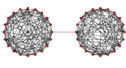
(a)

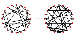
(b)

Figure 5: (a) An unweighted coupling graph with $40$ nodes, $201$ links, $\|G\|_{\mathcal{H}_{2}}=2.7837$, and $w_{\text{total}}(L)=201$. (b) An abstraction of Fig. 5(a) with $40$ nodes, $61$ links, $\|G_{s}\|_{\mathcal{H}_{2}}=3.0805$, and $w_{\text{total}}(L_{s})=199.88$.

In this section, we present several numerical examples to illustrate our theoretical findings.

\psfrag{y}[c][c]{\small Probability}\psfrag{x}[c][c]{\small Label of links}\includegraphics[trim=7.02625pt 7.02625pt 7.02625pt 7.02625pt,clip,width=225.48424pt]{probability_40_nodes_new.eps}

Figure 6: The probability of selecting a link of the coupling graph given by Fig. 5(a) as an important link. A cut edge is the most important link with the highest probability: if we throw out the cut edge, the coupling graph of the resulting abstraction will be disconnected for sure.

Example 1

We first consider a consensus network with $40$ agents defined over an unweighted coupling graph with two dense components which are connected by a single link, i.e., a cut edge. Each of the components is obtained by adding $100$ uniformly and randomly selected links to an empty graph with $20$ nodes; see Fig. 5(a). Based on Algorithm 1, we sample low-connectivity coupling links (i.e.,  feedback gains) with high probability and high-connectivity coupling links with low probability. The probability of selecting a link from the coupling graph is depicted in Fig. 6. One observes that the probability of selecting the cut edge as an important link is much higher than the probability of choosing other links. Fig. 5(b) shows a (0.5, 3.05)-abstraction of the network after applying Algorithm 1 that has $61$ links and meets all requirements of Definition 3. The coupling graph of the abstraction is weighted and has about 70% fewer links than the original network. Although, we set $\epsilon=0.5$ when running Algorithm 1, the performance loss of the resulting abstraction is less than $24$% according to Table II.

Systemic Performance Measure	$\frac{|{\Pi_{\rho}(L_{s})}-{\Pi_{\rho}(L)}|}{\Pi_{\rho}(L_{s})}\times 100$
System Hankel Norm: $\frac{1}{2}{\lambda_{2}}^{-1}$	19.65 %
Squared $\mathcal{H}_{2}$ Norm: $\frac{1}{2}\sum_{i=2}^{n}{\lambda_{i}}^{-1}$	18.34 %
Zeta Spectral Norm: $\Big{(}\sum_{i=2}^{n}{\lambda_{i}}^{-2}\Big{)}^{\frac{1}{2}}$	15.26 %
Local Deviation Error: $\frac{1}{2}\sum_{i\in\mathcal{V}}{d_{i}}^{-1}$	23.16 %

TABLE II: Relative performance loss percentage of network Fig. 5(a) with respect to its abstraction Fig. 5(b).

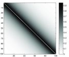
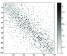
(a)	(b)

Figure 7: (a) This plot demonstrates the sparsity pattern of adjacency matrix of network in Example 2 with coupling parameters $c=1$ and $\gamma=0.05$. This network has $100$ agents and $4,950$ links and the color intensity at each pixel of this plot shows magnitude of the corresponding element in the adjacency matrix. (b) This plot depicts the sparsity pattern of adjacency matrix of an abstraction that has $1114$ links. The relative $\mathcal{H}_{2}$ error of these two networks is $\|G-G_{s}\|_{\mathcal{H}_{2}}/\|G\|_{\mathcal{H}_{2}}=0.18$ and the ratio of their total weights is $w_{\text{total}}(L_{s})/w_{\text{total}}(L)=1.0028$.

Systemic Performance Measure	$\frac{|{\Pi_{\rho}(L_{s})}-{\Pi_{\rho}(L)}|}{\Pi_{\rho}(L_{s})}\times 100$
System Hankel Norm: $\frac{1}{2}\lambda_{2}^{-1}$	10.72 %
Squared $\mathcal{H}_{2}$ Norm: $\frac{1}{2}\sum_{i=2}^{n}{\lambda_{i}}^{-1}$	6.44 %
Zeta Spectral Norm: $\Big{(}\sum_{i=2}^{n}{\lambda_{i}^{-2}}\Big{)}^{\frac{1}{2}}$	9.69 %
Local Deviation Error: $\frac{1}{2}\sum_{i\in\mathcal{V}}{d_{i}^{-1}}$	3.07 %

TABLE III: Relative performance loss percentage of network Fig. 7(a) with respect to its abstraction Fig. 7(b) that has $77.49$ % fewer links.

Example 2

Let us consider a consensus network with 100 agents and exponentially decaying couplings that are defined by

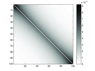
Figure 8: This plot presents the probability distribution of the sampling process to choose important links in Example 2. The color intensity of each pixel shows importance of that link for sampling.

$$w(\{i,j\})~{}=~{}\left\{\begin{array}[]{l l}c\hskip 1.42271pte^{-\gamma|i-j|}&\quad\text{if $i\neq j$}\\ 0&\quad\text{if $i=j$}\end{array}\right.$$ (97)

where $c$ and $\gamma$ are positive numbers and $i,j\in\mathcal{V}$. This class of networks arises in various applications where there is a notion of spatial distance between the subsystems; we refer to [18] for more details. Fig. 7(a) shows the adjacency matrix of the coupling graph of this network. According to Theorem 4, this network has a $(0.5,27.85)$-abstraction. Fig. 7(b) illustrates a $(0.5,22.28)$-abstraction of the network after applying Algorithm 1, where the design parameter $\epsilon$ is set to $0.5$. The original network has $4,950$ links, while its abstraction has $1,114$ coupling links and meets all requirements of Definition 3. As a result, abstraction achieves $77.49$ % sparsification. Although, in this example, we allow $50$% performance loss, numerous simulation examples assert that the resulting bounds for performance loss can be comparably smaller. As it is seen from Table III, the relative performance loss percentage is less than $11$%. Fig. 8 depicts the probability distribution of sampling process to select important links in Algorithm 1, where the color intensity of pixels show how important that link is. According to Algorithm 1, low-connectivity coupling links are sampled with higher probability than high-connectivity coupling links.

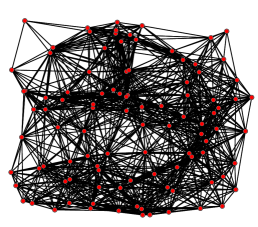
(a)

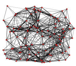
(b)

Figure 9: (a) An unweighted coupling (proximity) graph of a consensus network with $100$ agents is presented. Every agent is connected to all of its spatial neighbors within a closed ball of radius $r=10$. This graph has $1,291$ links and $w_{\text{total}}(L)=1,291$. (b) This graph shows a $(0.5,16.62)$-abstraction of the network. Our abstraction algorithm results in a network with a weighted coupling graph that has $831$ links and $w_{\text{total}}(L_{s})=1293.4$. The relative $\mathcal{H}_{2}$ error of these two networks is $\|G-G_{s}\|_{\mathcal{H}_{2}}/\|G\|_{\mathcal{H}_{2}}=0.17$.

Example 3

Let us consider a dynamical network consists of $100$ agents which are randomly distributed in a $30\times 30$ square-shape area in space and are coupled over a proximity graph. Every agent is connected to all of its spatial neighbors within a closed ball of radius $r=10$. Fig. 9(a) shows the resulting coupling graph of this dynamical network that has $100$ nodes and $1,291$ links and Fig. 9(b) depicts an$(0.5,16.62)$-abstraction of this network, which is obtained using Algorithm 1 with $\epsilon=0.5$. The number of coupling links in this abstraction is $831$, which is $35.63\%$ sparsification, and meets all requirements of Definition 3. Table IV summarizes the percentage of the relative performance loss with respect to some systemic performance measures.

Systemic Performance Measure	$\frac{|{\Pi_{\rho}(L_{s})}-{\Pi_{\rho}(L)}|}{\Pi_{\rho}(L_{s})}\times 100~{}$
Hankel Norm: $\frac{1}{2}{\lambda_{2}}^{-1}$	19.65 %
Squared $\mathcal{H}_{2}$-Norm: $\frac{1}{2}\sum_{i=2}^{n}{\lambda_{i}}^{-1}$	18.34 %
Zeta Spectral Norm: $\Big{(}\sum_{i=2}^{n}{\lambda_{i}^{-2}}\Big{)}^{\frac{1}{2}}$	15.26 %
Local Deviation Error: $\frac{1}{2}\sum_{i\in\mathcal{V}}{d_{i}^{-1}}$	23.16 %

TABLE IV: Relative performance loss percentage of network Fig. 9(a) with respect to its abstraction Fig. 9(b) that has $35.63\%$ fewer links.

Example 4

Let us consider a simple model for the formation control of a group of autonomous vehicles, which is given by

$$\left[\begin{array}[]{ccc}\dot{x}(t)\\ \dot{v}(t)\end{array}\right] = \left[\begin{array}[]{ccc}0&I\\ -L&-\beta L\end{array}\right]\left[\begin{array}[]{ccc}x(t)\\ v(t)\end{array}\right]+\left[\begin{array}[]{ccc}0\\ I\end{array}\right]\xi(t)$$ (106)

$$y(t) = M_{n}v(t)$$ (107)

where $\beta>0$ is a design parameter. Each vehicle has a position and a velocity variable. The state variable of the entire network is denoted by $[\begin{array}[]{cc}x(t)&v(t)\end{array}]^{\text{T}}$ and is measured relative to a pre-specified desired trajectory $x_{d}(t)$ and velocity $v_{d}(t)$. Without loss of generality, we may assume that the position and velocity of each vehicle are scalar variables. The reason is that one can decouple higher $D$-dimensional models into $D$ decoupled (106)-(107) models. The overall objective is for the network to reach a desired formation pattern, where each autonomous vehicle travels at the constant desired velocity $v_{d}$ while preserving a pre-specified distance between itself and each of its neighbors. In this model, the state feedback controller uses both position and velocity measurements and $L$ is, in fact, the corresponding feedback gain, which represents the coupling topology in the controller array, and constant $\beta$ is a design parameter [35, 28]. We consider the steady-state variance of the performance output of this network as the performance measure. This quantity is indeed equivalent to the square of the $\mathcal{H}_{2}$-norm of the system from the exogenous disturbance input to the performance output [28, 36, 37, 35, 38, 39]. The squared $\mathcal{H}_{2}$-norm of (106)-(107) can be characterized in terms of Laplacian eigenvalues of the coupling graph as follows

$$\Theta_{2}^{2}(L):=\lim_{t\rightarrow\infty}\mathbb{E}\left[y^{\text{T}}(t)y(t)\right]\,=\,\frac{1}{2\beta}\sum_{i=2}^{n}\lambda_{i}^{-2}\,=\,\frac{1}{2\beta}\,\zeta_{2}^{2}(L).$$ (108)

We refer to [11] for more details. This quantity is a homogeneous systemic performance measure; therefore, we can apply our abstraction algorithm. Suppose that the coupling graph of network (106)-(107) is given by Fig. 9(a). Then, as we mentioned in Example 3, Fig. 9(b) illustrates one example of $(0.5,16.62)$-abstraction of this network that is obtained using Algorithm 1. As shown in Example 3, this network has fewer coupling links ($831$ links) compare to the original network. Table V presents the percentage of the relative performance loss, where both systemic performance measures are homogeneous of order $-2$. This example shows that our proposed abstraction algorithm can be successfully applied to second-order linear consensus networks as well.

Systemic Performance Measure	$\frac{|{\Pi_{\rho}(L)}-{\Pi_{\rho}(L_{s})}|}{\Pi_{\rho}(L_{s})}\times 100~{}$
Squared $\mathcal{H}_{2}$-Norm: $\frac{1}{2\beta}\sum_{i=2}^{n}{\lambda_{i}^{-2}}$	17.58 %
Local Deviation Error: $\frac{1}{2\beta}\sum_{i=1}^{n}{d_{i}}^{-2}$	11.38 %

TABLE V: Relative performance loss percentage of network (106)-(107) with coupling graph Fig. 9(a) with respect to its abstraction Fig. 9(b).

X Discussion

We have introduced a notion of abstraction for a class of linear consensus networks based on notions of spectral sparsification. There have been several close-in-spirit notions of graph sparsifications in the context of theoretical computer science. While these other notions are interesting for their own sake from a combinatorial standpoint, their connections to performance analysis and synthesis of dynamical networks are not trivial and require further scrutiny. In this context, for a given graph there are several ways to define sparse subgraphs, namely, distance sparsifiers that approximate all pairwise distances up to a multiplicative and/or additive error (see [40] and subsequent research on spanners), cut sparsifiers that approximate every cut to an arbitrarily small multiplicative error [41], spectral sparsifier that approximate every eigenvalue to an arbitrarily small multiplicative error [31], and many more. It is shown that sparsifiers can be constructed by sampling links according to their strength, effective resistance [16], edge connectivity [32], or by sampling random spanning trees [42]. Benczúr and Karger propose a randomized algorithm to construct a cut sparsifier in $\mathcal{O}(m\log^{2}n)$ time for unweighted graphs and $\mathcal{O}(m\log^{3}n)$ time for weighted graphs [41, 32]. The notion of spectral sparsifier is stronger than cut sparsifier, which implies spectral sparsifiers are also cut sparsifiers. One of our current research directions is to investigate all these methods of sparsification and explore their connections to dynamical networks.

In our analysis, we assumed that the input matrix of the network is an identity matrix. Further extension of the current work includes linear consensus networks over directed coupling graphs with arbitrary input matrices. However, this generalization is challenging and even the problem formulation demands some appropriate conditions to guarantee the boundedness of performance measures.

Milad Siami received his dual B.Sc. degrees in electrical engineering and pure mathematics from Sharif University of Technology in 2009, M.Sc. degree in electrical engineering from Sharif University of Technology in 2011, and M.Sc. and Ph.D. degrees in mechanical engineering from Lehigh University in 2014 and 2017 respectively. From 2009 to 2010, he was a research student at the Department of Mechanical and Environmental Informatics at the Tokyo Institute of Technology, Tokyo, Japan. He is currently a postdoctoral associate in the Institute for Data, Systems, and Society at MIT. His research interests include distributed control systems, distributed optimization, and applications of fractional calculus in engineering. He received a Gold Medal of National Mathematics Olympiad, Iran (2003) and the Best Student Paper Award at the 5th IFAC Workshop on Distributed Estimation and Control in Networked Systems (2015). Moreover, he was awarded RCEAS Fellowship (2012), Byllesby Fellowship (2013), Rossin College Doctoral Fellowship (2015), and Graduate Student Merit Award (2016) at Lehigh University.

Nader Motee (S’99-M’08-SM’13) received his B.Sc. degree in Electrical Engineering from Sharif University of Technology in 2000, M.Sc. and Ph.D. degrees from University of Pennsylvania in Electrical and Systems Engineering in 2006 and 2007 respectively. From 2008 to 2011, he was a postdoctoral scholar in the Control and Dynamical Systems Department at Caltech. He is currently an Associate Professor in the Department of Mechanical Engineering and Mechanics at Lehigh University. His current research area is distributed dynamical and control systems with particular focus on issues related to sparsity, performance, and robustness. He is a past recipient of several awards including the 2008 AACC Hugo Schuck best paper award, the 2007 ACC best student paper award, the 2008 Joseph and Rosaline Wolf best thesis award, a 2013 Air Force Office of Scientific Research Young Investigator Program award (AFOSR YIP), a 2015 NSF Faculty Early Career Development (CAREER) award, and a 2016 Office of Naval Research Young Investigator Program award (ONR YIP).

References

- [1] M. Siami and N. Motee, “Systemic measures for performance and robustness of large–scale interconnected dynamical networks,” in Proceedings of the 53rd IEEE Conference on Decision and Control, Dec. 2014, pp. 5119–5124.
- [2] ——, “Schur–convex robustness measures in dynamical networks,” in Proceedings of the 2014 American Control Conference, 2014, pp. 5198–5203.
- [3] R. Olfati-Saber and R. Murray, “Consensus problems in networks of agents with switching topology and time-delays,” IEEE Transactions on Automatic Control, vol. 49, no. 9, pp. 1520–1533, Sept 2004.
- [4] M. Siami and N. Motee, “Robustness and performance analysis of cyclic interconnected dynamical networks,” in Proceedings of the 2013 SIAM Conference on Control and Its Application, Jan. 2013, pp. 137–143.
- [5] M. Fardad, F. Lin, and M. R. Jovanović, “Design of optimal sparse interconnection graphs for synchronization of oscillator networks,” IEEE Transactions on Automatic Control, vol. 59, no. 9, pp. 2457–2462, 2014.
- [6] T. H. Summers, F. L. Cortesi, and J. Lygeros, “On submodularity and controllability in complex dynamical networks,” IEEE Transactions on Control of Network Systems, vol. 3, no. 1, pp. 91–101, March 2016.
- [7] A. Girard and G. J. Pappas, “Approximation metrics for discrete and continuous systems,” IEEE Transactions on Automatic Control, vol. 52, no. 5, pp. 782–798, May 2007.
- [8] S. Gugercin, A. C. Antoulas, and C. Beattie, “ model reduction for large-scale linear dynamical systems,” SIAM Journal on Matrix Analysis and Applications, vol. 30, no. 2, pp. 609–638, 2008.
- [9] B. Moore, “Principal component analysis in linear systems: Controllability, observability, and model reduction,” IEEE Transactions on Automatic Control, vol. 26, no. 1, pp. 17–32, Feb 1981.
- [10] M. Johansson and A. Rantzer, “Computation of piecewise quadratic lyapunov functions for hybrid systems,” IEEE Transactions on Automatic Control, vol. 43, no. 4, pp. 555–559, Apr 1998.
- [11] M. Siami and N. Motee, “Fundamental limits on robustness measures in networks of interconnected systems,” in Proceedings of the 52nd IEEE Conference on Decision and Control, Dec. 2013, pp. 67–72.
- [12] ——, “Fundamental limits and tradeoffs on disturbance propagation in linear dynamical networks,” IEEE Transactions on Automatic Control, vol. 61, no. 12, pp. 4055–4062, 2016.
- [13] X. Wu and M. R. Jovanović, “Sparsity-promoting optimal control of consensus and synchronization networks,” in Proceedings of the 2014 American Control Conference, 2014, pp. 2948–2953.
- [14] S. Hassan-Moghaddam and M. R. Jovanović, “An interior point method for growing connected resistive networks,” in Proceedings of the 2015 American Control Conference, Chicago, IL, 2015, pp. 1223–1228.
- [15] N. Dhingra, F. Lin, M. Fardad, and M. R. Jovanović, “On identifying sparse representations of consensus networks,” IFAC Proceedings Volumes, vol. 45, no. 26, pp. 305 – 310, 2012.
- [16] D. A. Spielman and N. Srivastava, “Graph sparsification by effective resistances,” in Proceedings of the 14th Annual ACM Symposium on Theory of Computing, ser. STOC ’08. New York, NY, USA: ACM, 2008, pp. 563–568.
- [17] J. Batson, D. Spielman, and N. Srivastava, “Twice-ramanujan sparsifiers,” SIAM Review, vol. 56, no. 2, pp. 315–334, 2014.
- [18] N. Motee and Q. Sun, “Sparsity and spatial localization measures for spatially distributed systems,” SIAM Jounal on Control and Optimization, vol. 55, no. 1, pp. 200–235, 2017.
- [19] C. Chen, G. Iyengar, and C. C. Moallemi, “An axiomatic approach to systemic risk,” Management Science, vol. 59, no. 6, pp. 1373–1388, 2013.
- [20] M. Siami and N. Motee, “Growing linear consensus networks via systemic performance measures,” IEEE Transactions on Automatic Control, Submitted, 2016.
- [21] S. Hawking, “Zeta function regularization of path integrals in curved space-time,” Communications in Mathematical Physics, vol. 133, no. 55, 1977.
- [22] V. D. Blondel, E. D. Sontag, M. Vidyasagar, and J. C. Willems, Open Problems in Mathematical Systems and Control Theory. Springer Verlag, 1999.
- [23] S. Boyd, L. E. Ghaoui, E. Feron, and V. Balakrishnan, Linear Matrix Inequalities in System and Control Theory. Society for Industrial Mathematics, 1997.
- [24] M. H. de Badyn, A. Chapman, and M. Mesbahi, “Network entropy: A system-theoretic perspective,” in Proceedings of 54th IEEE Conference Decision and Control, Dec 2015, pp. 5512–5517.
- [25] K. Glover, “All optimal hankel-norm approximations of linear multivariable systems and their l, ∞ -error bounds†,” International Journal of Control, vol. 39, no. 6, pp. 1115–1193, 1984.
- [26] J. Borwein and A. Lewis, Convex Analysis and Nonlinear Optimization: Theory and Examples, ser. CMS Books in Mathematics. Springer New York, 2005.
- [27] S. Boyd., “Convex optimization of graph laplacian eigenvalues,” in Proceedings International Congress of Mathematicians, 2006, pp. 1311–1319.
- [28] B. Bamieh, M. Jovanović, P. Mitra, and S. Patterson, “Coherence in large-scale networks: Dimension-dependent limitations of local feedback,” IEEE Transactions on Automatic Control, vol. 57, no. 9, pp. 2235 –2249, sept. 2012.
- [29] M. Newman, The Laplacian Spectrum of Graphs. University of Manitoba, 2001.
- [30] M. Rudelson and R. Vershynin, “Sampling from large matrices: An approach through geometric functional analysis,” Journal of the ACM, vol. 54, no. 4, Jul. 2007. [Online]. Available: http://doi.acm.org/10.1145/1255443.1255449
- [31] D. A. Spielman and S.-H. Teng, “Nearly-linear time algorithms for graph partitioning, graph sparsification, and solving linear systems,” in Proceedings of the Thirty-sixth Annual ACM Symposium on Theory of Computing, ser. STOC ’04. New York, NY, USA: ACM, 2004, pp. 81–90.
- [32] W. S. Fung, R. Hariharan, N. J. Harvey, and D. Panigrahi, “A general framework for graph sparsification,” in Proceedings of the Forty-third Annual ACM Symposium on Theory of Computing, ser. STOC ’11. New York, NY, USA: ACM, 2011, pp. 71–80. [Online]. Available: http://doi.acm.org/10.1145/1993636.1993647
- [33] J. Doyle, K. Glover, P. Khargonekar, and B. Francis, “State-space solutions to standard and control problems,” IEEE Transactions on Automatic Control, vol. 34, no. 8, pp. 831–847, Aug 1989.
- [34] R. Arastoo, M. Bahavarnia, M. V. Kothare, and N. Motee, “Closed-loop feedback sparsification under parametric uncertainties,” in 2016 IEEE 55th Conference on Decision and Control (CDC), Dec 2016, pp. 123–128.
- [35] S. Patterson and B. Bamieh, “Network coherence in fractal graphs,” in Decision and Control and European Control Conference (CDC-ECC), 2011 50th IEEE Conference on, Dec. 2011, pp. 6445–6450.
- [36] G. F. Young, L. Scardovi, and N. E. Leonard, “Robustness of noisy consensus dynamics with directed communication,” in American Control Conference (ACC), 2010, July 2010, pp. 6312–6317.
- [37] A. Jadbabaie and A. Olshevsky, “Combinatorial bounds and scaling laws for noise amplification in networks,” in European Control Conference (ECC), July 2013, pp. 596–601.
- [38] B. Bamieh and D. Gayme, “The price of synchrony: Resistive losses due to phase synchronization in power networks,” in American Control Conference (ACC), 2013, September 2012, pp. 5815–5820.
- [39] E. Lovisari, F. Garin, and S. Zampieri, “Resistance-based performance analysis of the consensus algorithm over geometric graphs,” SIAM Journal on Control and Optimization, vol. 51, no. 5, pp. 3918–3945, 2013.
- [40] D. Peleg and A. A. Schäffer, “Graph spanners,” Journal of Graph Theory, vol. 13, no. 1, pp. 609–638, 1989.
- [41] A. A. Benczúr and D. R. Karger, “Approximating s-t minimum cuts in Õ(n2) time,” in Proceedings of the Twenty-eighth Annual ACM Symposium on Theory of Computing, ser. STOC ’96. New York, NY, USA: ACM, 1996, pp. 47–55. [Online]. Available: http://doi.acm.org/10.1145/237814.237827
- [42] N. Goyal, L. Rademacher, and S. Vempala, “Expanders via random spanning trees,” in Proceedings of the Twentieth Annual ACM-SIAM Symposium on Discrete Algorithms, ser. SODA ’09. Philadelphia, PA, USA: Society for Industrial and Applied Mathematics, 2009, pp. 576–585.