CMB anisotropies from patchy reionisation and diffuse Sunyaev-Zel’dovich effects

Abstract

Anisotropies in the Cosmic Microwave Background (CMB) can be induced during the later stages of cosmic evolution, and in particular during and after the Epoch of Reionisation. Inhomogeneities in the ionised fraction, but also in the baryon density, in the velocity fields and in the gravitational potentials are expected to generate correlated CMB perturbations. We present a complete relativistic treatment of all these effects, up to second order in perturbation theory, that we solve using the numerical Boltzmann code Song. The physical origin and relevance of all second order terms are carefully discussed. In addition to collisional and gravitational contributions, we identify the diffuse analogue of the blurring and kinetic Sunyaev-Zel’dovich (SZ) effects. Our approach naturally includes the correlations between the imprint from patchy reionisation and the diffuse SZ effects thereby allowing us to derive reliable estimates of the induced temperature and polarisation CMB angular power spectra. In particular, we show that the $B$-modes generated at intermediate length-scales ($\ell\simeq 100$) have the same amplitude as the $B$-modes coming from primordial gravitational waves with a tensor-to-scalar ratio $r=10^{-4}$.

1 Introduction

The cosmic microwave background (CMB) has been exploited with great success in the past decades and remains the main pillar of precision cosmology. Beyond the linear physics in the era of recombination, a large range of secondary effects are present which are crucial for the analysis of current and future missions [1, 2, 3, 4, 5, 6]. In addition to constituting a “background” to the purely linear physics, they also carry information about the cosmic evolution itself [7]. Secondary effects appear both at linear and non-linear order in the theory of the cosmological perturbations. The linear ones are the late Integrated Sachs-Wolfe effect (ISW) and Doppler effect from collisions after reionisation. These ones are implemented in most linear Boltzmann codes currently available and will not be discussed in the following [8, 9, 10]. Non-linear secondaries can be separated into different classes:

1. Gravitational dynamics. General Relativity induces CMB perturbations going beyond the linear ISW and SW effects. These are called the Rees-Sciama effects [11] and are typically negligible compared to the remaining secondaries [12, 13].

2. Line-of-sight distortions. Gravitational effects bend the light rays. This includes the gravitational lensing [14, 15, 16], but also time-delay [17] and redshift effects as discussed in Refs. [18, 19, 20]. Lensing is an important and observable effect, while the latter ones are subleading [21, 20].

3. Collisional dynamics at recombination. Contributions beyond the linear collision term, as for example higher order phase-space enhancements [22, 18, 19]. The effect is of intermediate size and is slightly below the Planck satellite detection sensitivity [23].

4. Collisional dynamics at the Epoch of Reionisation. The same physics at work during recombination becomes relevant again during the Epoch of Reionisation (EoR) [24, 25]. Since reionisation is a completely inhomogeneous process, the impact of second-order corrections is enhanced. The two main contributions are the blurring of existing CMB anisotropies due to the ionised gas [26] and the induction of perturbations by collisions [27, 28]. This signal is expected to be a direct probe of the EoR [29].

5. Collisional dynamics after EoR. Once reionisation is completed, the Universe is fully ionised and CMB photons may scatter with the free electrons. Collisions are most likely in overdense regions and the resulting imprints in the CMB are known as the Sunyaev-Zel’dovich (SZ) effects. As for the reionisation contribution, we distinguish between the less studied blurring effects [30] and the well-known collision-induced CMB perturbations [31, 32, 33]. Of especial interest is the generation of polarisation from the SZ effects [34]. Let us stress that, in our case, collisions are not only occurring in dense galactic clusters but are diffuse over the whole Universe.

In this paper we attempt to include these CMB secondaries in the theory of the cosmological perturbations at second order. Such a treatment has originally been proposed by Hu, Scott and Silk in Ref. [35], but this work was dedicated to the small scale temperature anisotropies, considering only the most dominant contributions. Our work therefore extends these results to the full sky, encompassing the entire range of second order sources and, more importantly, to the $E$- and $B$-mode polarisation.

In the past years several second-order Boltzmann codes have been developed [22, 18, 19] that can accurately compute the effects discussed in point 1) and 3), plus the redshift effects from point 2). Lensing is already treated in linear codes such as Camb [8] or Class [10]. However, the terms discussed in the points 4) and 5) have not be considered. We focus on their implementation in the Boltzmann code Song [19], in full General Relativity and only employing the assumption of neglecting third and higher order corrections.

The paper is organised as follows. Key results from second-order perturbation theory are reviewed in section 2 while we detail our numerical implementation in section 3. Numerical calculations of the temperature and polarisation power spectra are presented in section 4. We conclude in section 5.

2 Second order perturbation theory

In the following we introduce our notation and review some results from the theory of the cosmological perturbations at second-order.

2.1 Notation

Greek indices $\mu,\nu$ label a relativistic 4-vector, while indices $\alpha,\beta$ describe a special relativistic 4-vector (for example in the local inertial frame). Latin indices $i,j$ refer to the spatial parts of both relativistic and special relativistic vectors, while the temporal index is labelled by a $0$. Latin indices $a,b$ are helicity indices and run over $a=\pm$ for photons.

The metric is assumed to be of the form

$$ds^{2}=a^{2}\left\{(1+2A){\mathrm{d}}\eta^{2}+2B_{i}{\mathrm{d}}\eta{\mathrm{d}}x^{i}-\left[(1+2D)\delta_{ij}+2E_{ij}\right]{\mathrm{d}}x^{i}{\mathrm{d}}x^{j}\right\},$$ (2.1)

with the lapse perturbation $A$, the shift ${\boldsymbol{B}}\equiv\{B^{i}\}$, the spatial trace perturbation $D$ and the symmetric spatial tensor perturbation $E_{ij}$. Einstein equations, stress tensor and Boltzmann equations are then expanded to second-order in perturbation theory $X=X^{(1)}+X^{(2)}+\cdots$. We further assume that $B_{i}^{(1)}=E^{(1)}_{ij}=0$, corresponding to the so-called Poisson gauge at linear order, plus the assumption that vector and tensor modes, for example due to primordial gravitational waves, are counted as a second-order perturbation.

The stress tensor is decomposed as

$$T_{\mu\nu}=(\rho+P)u_{\mu}u_{\nu}-Pg_{\mu\nu}+\Sigma_{\mu\nu}\,,$$ (2.2)

where $\rho$ is the density, $P$ the pressure, $\Sigma_{\mu\nu}$ the anisotropic stress tensor and $u_{\mu}$ the rest-frame 4-velocity.

We characterise the species in the Universe by their distribution function $f_{ab}(\eta,{\boldsymbol{x}},{\boldsymbol{p}})$; the probability of finding a particle of a given species with 3-momentum ${\boldsymbol{p}}$ at the position ${\boldsymbol{x}}$ and conformal time $\eta$. The stress tensor can be built from the distribution function by evaluating the first kinetic moments

$$T_{\mu\nu}=[e^{\alpha}]_{\mu}[e^{\beta}]_{\nu}\int\dfrac{{\mathrm{d}}{\boldsymbol{p}}}{(2\pi)^{3}}f(\eta,{\boldsymbol{x}},{\boldsymbol{p}})\frac{p_{\alpha}p_{\beta}}{p_{0}}\,,$$ (2.3)

where $[e^{\alpha}]_{\mu}$ stands for the tetrad and $p_{0}$ is the rest frame energy.

Cold species, such as massive particles, have a trivial phase-space and all information is contained in the first moments: the density $\rho$ and the 3-velocity ${\boldsymbol{v}}$. The latter being defined as the spatial part of $u$ at linear order $v^{(1)}_{i}\equiv au^{(1)}_{i}$. Relativistic species, however, require the knowledge of the distribution function. When not interested in the spectral information, one may integrate over the momentum and we define

$$\Delta_{ab}(\eta,{\boldsymbol{x}},{\boldsymbol{n}})\equiv\dfrac{\int{\mathrm{d}}qq^{3}f_{ab}(\eta,x,q{\boldsymbol{n}})}{\int{\mathrm{d}}qq^{3}f_{I}^{(0)}(q)}\,,$$ (2.4)

where $q_{i}=ap_{i}$ is the comoving momentum of direction ${\boldsymbol{n}}$ and magnitude $q$. These quantities are sufficient to evaluate the stress tensor and to provide a closed set of equations. The $\Delta_{ab}$ can be related to the temperature of an equivalent blackbody spectrum.

We use the Fourier conventions

$$A({\boldsymbol{x}})=\int\frac{{\mathrm{d}}^{3}{\boldsymbol{k}}}{(2\pi)^{3}}e^{i{\boldsymbol{k}}\cdot{\boldsymbol{x}}}A({\boldsymbol{k}})\,,$$ (2.5)

while all multiplications involving different wavenumbers in Fourier space are implicitly assumed to be convolution integrals, namely

$$A({\boldsymbol{k}}_{1})B({\boldsymbol{k}}_{2})\equiv\int\dfrac{{\mathrm{d}}^{3}{\boldsymbol{k}}_{1}}{(2\pi)^{3}}\int\dfrac{{\mathrm{d}}^{3}{\boldsymbol{k}}_{2}}{(2\pi)^{3}}(2\pi)^{3}\delta^{3}({\boldsymbol{k}}-{\boldsymbol{k}}_{1}-{\boldsymbol{k}}_{2})A({\boldsymbol{k}}_{1})B({\boldsymbol{k}}_{2})\,.$$ (2.6)

Multipole decomposition is assumed to be a decomposition over the spin-weighted spherical harmonics as

$$f_{ab}(\eta,{\boldsymbol{x}},{\boldsymbol{q}})=\sum\limits_{l,m}(-i)^{l}\sqrt{\frac{4\pi}{2l+1}}f_{ab,lm}(\eta,{\boldsymbol{k}},q)Y_{lm}^{s}({\boldsymbol{n}})\,.$$ (2.7)

Here, $s$ is the spin associated with the helicity state $ab$ and $Y_{lm}^{s}$ are the spin-weighted spherical harmonics. Note that $ab$ is usually decomposed into the Stokes parameters $X=I,V,Q,U$ before multipole decomposition, or into $X=I,V,E,B$ after multipole decomposition.

Similarly to our notation for the convolutions, an implicit summation at fixed $m$ is assumed over all multipole coefficients labelled with $m_{1}$ or $m_{2}\equiv m-m_{1}$. Finally, indices within square bracket refer to helicity states. Further details are given in Refs. [36, 37].

2.2 Line-of-Sight integration

The line-of-sight integration is an important tool for solving the Boltzmann equations. It analytically describes the generation of the large present-day multipoles from sources active at much lower multipoles. Thereby it makes possible the truncation of the Boltzmann hierarchy at a given multipole $l$; higher multipole moments being compensated by using an analytical expression [38, 39]. Let us assume a differential equation in Fourier space of the form

$$\dot{\Delta}_{ab}+i{\boldsymbol{n}}\cdot{\boldsymbol{k}}\Delta_{ab}=-|\dot{\kappa}|\Delta_{ab}+\rho_{ab}\,,$$ (2.8)

where the term $i{\boldsymbol{n}}\cdot{\boldsymbol{k}}\Delta_{ab}$ describes the free propagation of photons, $|\dot{\kappa}|$ is the chance for interactions and consequently $-|\dot{\kappa}|\Delta_{ab}$ describes collisions knocking the photons out of our line-of-sight. The rightmost quantity, $\rho_{ab}$, contains all remaining terms that are found in the full second-order equations. The solution to this equation is formally given by

$$\Delta_{ab}(\eta,{\boldsymbol{k}},{\boldsymbol{n}})=\int\limits_{\eta_{\mathrm{ini}}}^{\eta}{\mathrm{d}}\eta^{\prime}e^{-i{\boldsymbol{n}}\cdot{\boldsymbol{k}}(\eta-\eta^{\prime})-\kappa(\eta,\eta^{\prime})}\rho_{ab}(\eta^{\prime},{\boldsymbol{k}},{\boldsymbol{n}})\,,$$ (2.9)

where $\kappa$ is the integrated optical depth and the exponential $e^{-i{\boldsymbol{n}}\cdot{\boldsymbol{k}}(\eta-\eta^{\prime})}$ describes the generation of a more complex angular distribution by the free propagation of photons. The multipole decomposition of this equation is non-trivial and can be found in Ref. [36].

2.3 Collision terms at second order

The polarised second-order Boltzmann equations have been derived in Refs. [40, 36] and contain numerous sources, including the lensing and gravitational ones. In the following, we explicitly write the source terms that are only due to interactions, namely, the ones appearing in the second-order collision term [37]. For the intensity, they read

$$C^{(2)}_{Ilm} =|\dot{\kappa}|\bigg{(}-\Delta_{I,lm}^{(2)}({\boldsymbol{k}})+\delta_{l0}\Delta_{I,00}^{(2)}({\boldsymbol{k}})+4\delta_{l1}v_{\mathrm{b},[m]}^{(2)}({\boldsymbol{k}})+\delta_{l2}\frac{1}{10}\left[\Delta_{I,2m}^{(2)}({\boldsymbol{k}})-\sqrt{6}\Delta_{E,2m}^{(2)}({\boldsymbol{k}})\right]$$

$$+\left[A^{(1)}({\boldsymbol{k}}_{1})+\delta_{\mathrm{b}}^{(1)}({\boldsymbol{k}}_{1})+\delta_{x_{\mathrm{e}}}^{(1)}({\boldsymbol{k}}_{1})\right]$$

$$\times\bigg{\{}-\Delta_{I,lm}^{(1)}({\boldsymbol{k}}_{2})+\delta_{l0}\Delta_{I,00}^{(1)}({\boldsymbol{k}}_{2})+4\delta_{l1}v_{\mathrm{b},[m]}^{(1)}({\boldsymbol{k}}_{2})+\delta_{l2}\frac{1}{10}\left[\Delta_{I,2m}^{(1)}({\boldsymbol{k}}_{2})-\sqrt{6}\Delta_{E,2m}^{(1)}({\boldsymbol{k}}_{2})\right]\bigg{\}}$$

$$+\sum_{\epsilon=\pm}(-\epsilon)v^{(1)}_{\mathrm{b},[m_{2}]}({\boldsymbol{k}}_{1})\Delta_{I,(l+\epsilon)m_{1}}^{(1)}({\boldsymbol{k}}_{2})C^{\epsilon,l}_{m_{1}m}$$

$$+\delta_{l0}\,v^{(1)}_{\mathrm{b},[m_{2}]}({\boldsymbol{k}}_{1})\left[2\Delta_{I,1m_{1}}^{(1)}({\boldsymbol{k}}_{2})-4v^{(1)}_{\mathrm{b},[m_{1}]}({\boldsymbol{k}}_{2})\right]C^{+,0}_{m_{1}m}$$

$$+3\delta_{l1}\,v^{(1)}_{\mathrm{b},[m_{2}]}({\boldsymbol{k}}_{1})\Delta_{I,0m_{1}}^{(1)}({\boldsymbol{k}}_{2})C^{-,1}_{m_{1}m}+\delta_{l2}\,v^{(1)}_{\mathrm{b},[m_{2}]}({\boldsymbol{k}}_{1})\left[7v^{(1)}_{\mathrm{b},[m_{1}]}({\boldsymbol{k}}_{2})-\frac{1}{2}\Delta_{I,1m_{1}}^{(1)}({\boldsymbol{k}}_{2})\right]C^{-,2}_{m_{1}m}$$

$$+\frac{1}{2}\delta_{l3}\,v^{(1)}_{\mathrm{b},[m_{2}]}({\boldsymbol{k}}_{1})\left[\Delta_{I,2m_{1}}^{(1)}({\boldsymbol{k}}_{2})-\sqrt{6}\Delta_{E,2m_{1}}^{(1)}({\boldsymbol{k}}_{2})\right]C^{-,3}_{m_{1}m}\bigg{)}.$$ (2.10)

For the $E$-mode polarisation, they are

$$C^{(2)}_{Elm} =|\dot{\kappa}|\bigg{(}-\Delta_{E,lm}^{(2)}({\boldsymbol{k}})-\delta_{l2}\frac{\sqrt{6}}{10}\left[\Delta_{I,2m}^{(2)}({\boldsymbol{k}})-\sqrt{6}\Delta_{E,2m}^{(2)}({\boldsymbol{k}})\right]$$ (2.11)

$$+\left[A^{(1)}({\boldsymbol{k}}_{1})+\delta_{\mathrm{b}}^{(1)}({\boldsymbol{k}}_{1})+\delta_{x_{\mathrm{e}}}^{(1)}({\boldsymbol{k}}_{1})\right]$$

$$\times\bigg{\{}-\Delta_{E,lm}^{(1)}({\boldsymbol{k}}_{2})-\delta_{l2}\frac{\sqrt{6}}{10}\left[\Delta_{I,2m}^{(1)}({\boldsymbol{k}}_{2})-\sqrt{6}\Delta_{E,2m}^{(1)}({\boldsymbol{k}}_{2})\right]\bigg{\}}$$

$$+\sum_{\epsilon=\pm}(-\epsilon)v^{(1)}_{\mathrm{b},[m_{2}]}({\boldsymbol{k}}_{1})\Delta_{E,(l+\epsilon)m_{1}}^{(1)}({\boldsymbol{k}}_{2})D^{\epsilon,l}_{m_{1}m}$$

$$+\delta_{l2}\frac{\sqrt{6}}{2}v^{(1)}_{\mathrm{b},[m_{2}]}({\boldsymbol{k}}_{1})\left[\Delta_{I,1m_{1}}^{(1)}({\boldsymbol{k}}_{2})-2v^{(1)}_{\mathrm{b},[m_{1}]}({\boldsymbol{k}}_{2})\right]C_{m_{1}m}^{-,2}$$

$$-\delta_{l3}\frac{\sqrt{6}}{2}v^{(1)}_{\mathrm{b},[m_{2}]}({\boldsymbol{k}}_{1})\left[\Delta_{I,2m_{1}}^{(1)}({\boldsymbol{k}}_{2})-\sqrt{6}\Delta_{E,2m_{1}}^{(1)}({\boldsymbol{k}}_{2})\right]D^{-,3}_{m_{1}m}\bigg{)},$$

while the $B$-mode terms read

$$C^{(2)}_{Blm} =|\dot{\kappa}|\bigg{\{}-\Delta_{B,lm}^{(2)}({\boldsymbol{k}})+v^{(1)}_{\mathrm{b},[m_{2}]}({\boldsymbol{k}}_{1})\Delta_{E,lm_{1}}^{(1)}({\boldsymbol{k}}_{2})D^{0,l}_{m_{1}m}$$ (2.12)

$$-\delta_{l2}\frac{\sqrt{6}}{5}v^{(1)}_{\mathrm{b},[m_{2}]}({\boldsymbol{k}}_{1})\left[\Delta_{I,2m_{1}}^{(1)}({\boldsymbol{k}}_{2})-\sqrt{6}\Delta_{E,2m_{1}}^{(1)}({\boldsymbol{k}}_{2})\right]D^{0,2}_{m_{1}m}\,\bigg{\}}.$$

In the previous three equations, the quantities $C^{\pm,l}_{mm^{\prime}}$, $D^{\pm,l}_{mm^{\prime}}$ and $D^{0,l}_{mm^{\prime}}$ are the coupling functions, which are specific combinations of the Clebsch-Gordan coefficients. They are given in the appendix A of Ref. [37]. Note that we have assumed a cold ensemble of electrons and are therefore not considering thermal contributions, such as the thermal Sunyaev-Zel’dovich effect.

In Eqs. (2.10), (2.11), and (2.12), the first terms, of the form $-|\dot{\kappa}|\Delta^{(2)}_{Xlm}$, describe scatterings out of the line-of-sight and are straightforwardly integrated as an exponential term in Eq. (2.9). All the other terms however have to be accounted for as new collisional sources and add-up to form the term $\rho_{ab}$ in Eq. (2.9). In addition, while the sources are very different for the $E$- and $B$-mode polarisation, these modes do mix in free-streaming. For practical purposes we therefore do not refer to $E$- or $B$-mode sources separately, instead they will be referred to as the polarised sources.

In the following, we discuss the origin of all these quantities and this allows us to distinguish three categories.

2.3.1 Pure terms

We label as “pure” the terms which contain only a single second-order perturbation. These ones assume a functional form identical to the linear collision term, $C^{(1)}_{X,lm}$, but with the second-order perturbations instead of the first order ones. For the intensity, one obtains from Eq. (2.10)

$$C^{(2)}_{I,\mathrm{pure}}=|\dot{\kappa}|\,\left\{-\Delta_{I,lm}^{(2)}({\boldsymbol{k}})+\delta_{l0}\Delta_{I,00}^{(2)}({\boldsymbol{k}})+4\delta_{l1}v_{\mathrm{b},[m]}^{(2)}({\boldsymbol{k}})+\delta_{l2}\frac{1}{10}\left[\Delta_{I,2m}^{(2)}({\boldsymbol{k}})-\sqrt{6}\Delta_{E,2m}^{(2)}({\boldsymbol{k}})\right]\right\}.$$ (2.13)

As above-mentioned, the first term accounts for collisions out of our line-of-sight and has to be discarded from $\rho_{ab}$ as it is already included in the line-of-sight integration. Next we have a monopole term and the generation of a dipole aligned with the second-order baryon velocity. Finally, there is a quadrupole emission that also generates $E$-mode polarisation.

Although the pure terms describe the same physics as the well-known linear collision terms, they do involve the cosmological perturbations at second order. As such, they can be affected by more complex phenomena than their linear counterparts. For instance, lensing might change the multipole moments before reionisation and thereby change the likelihood of collisions at reionisation and later. As a result, the pure terms can be affected by all possible second-order sources prior to the collision and this requires a different numerical treatment than the other terms discussed below. Let us remark that the pure terms are defined due to these numerical considerations and do not represent a specific physical process.

2.3.2 Gain terms

The gain terms describe the generation of perturbations by outgoing photons that end up being scattered into our line-of-sight. Ignoring the pure terms in $C^{(2)}_{X}$, the gain terms can be identified by remarking that they should be quadratic in the linear perturbations and linked to a given low multipole. The reason being that photons emitted after a collision follow a simple angular distribution, dictated by the kinematics of the collision. For Compton scattering this corresponds to a dipole aligned with the direction of the electron velocity.

During the evolution of the Universe, the photon power streams to smaller scales, suppressing the low multipoles, while the baryon perturbations grow. As a consequence, terms that are quadratic in the linear baryon perturbations are expected to dominate over the remaining sources. As such, the most important gain terms are the ones that involve the baryon density contrast $\delta_{\mathrm{b}}$. These represent the Sunyaev-Zel’dovich (SZ) effect [31]

$$C^{(2)}_{I,\mathrm{SZ}}=|\dot{\kappa}|\delta^{(1)}_{\mathrm{b}}({\boldsymbol{k}}_{1})\left\{\delta_{l0}\Delta_{I,00}^{(1)}({\boldsymbol{k}})+4\delta_{l1}v_{\mathrm{b},[m]}^{(1)}({\boldsymbol{k}})+\delta_{l2}\frac{1}{10}\left[\Delta_{I,2m}^{(1)}({\boldsymbol{k}})-\sqrt{6}\Delta_{E,2m}^{(1)}({\boldsymbol{k}})\right]\right\}.$$ (2.14)

The SZ effect describes the inhomogeneously increased likelihood of collisions in overdense regions of the Universe. It is particularly enhanced for very massive, isolated structures, such as the galaxy clusters [41]. Here we only treat the second-order part of this effect, also known as the Ostriker-Vishniac effect [32, 42, 33], while the sources are all the inhomogeneities in the late-time Universe. For this reason, we will be referring to it as the diffuse SZ effect.

The structure of the diffuse SZ effect is a convolution between the baryon overdensity and the linear collision gain term. The most important contribution is the second term involving the baryon velocity $v_{\mathrm{b}}$. This is the so-called kinematic Sunyaev-Zel’dovich effect (kSZ), which describes an alignment of the outgoing photons with the baryon velocity. The remaining terms are the generation of a homogeneous monopole radiation (0SZ) and a quadrupole (2SZ). For the $E$-mode polarisation we find a similar quadrupole contribution (pSZ), which describes that an already existing temperature quadrupole may be re-scattered in the late Universe and converted into polarisation. The pSZ terms are the diffuse version of the exact same polarization induced signals that have been discussed for galaxy clusters, see for instance Refs. [34, 43, 44, 45, 46].

In the standard treatment, the SZ effect is usually first evaluated in the local rest frame of a galaxy cluster and one has to correct from its local motion with respect to the CMB frame. For the diffuse SZ effect, this is not the case as we simulate the entire Universe already. The above equations have been derived in the frame in which the CMB dipole has no expectation value. As such, the corrections describing the impact of the relative motion compared to the local CMB dipole are very small and would only appear at third-order in perturbation theory.

As it can be seen from the full Eq. (2.10), the exact same terms multiplying $\delta_{\mathrm{b}}^{(1)}$ in Eq. (2.14) appear convolved with the gravitational potential perturbation $A^{(1)}$ and the inhomogeneities in the ionised fraction $\delta_{x_{\mathrm{e}}}^{(1)}$. For the intensity, in addition to SZ, we therefore have the following gain terms

$$C^{(2)}_{I,\mathrm{EoR}} =|\dot{\kappa}|\delta_{x_{\mathrm{e}}}^{(1)}({\boldsymbol{k}}_{1})\left\{\delta_{l0}\Delta_{I,00}^{(1)}({\boldsymbol{k}})+4\delta_{l1}v_{\mathrm{b},[m]}^{(1)}({\boldsymbol{k}})+\delta_{l2}\frac{1}{10}\left[\Delta_{I,2m}^{(1)}({\boldsymbol{k}})-\sqrt{6}\Delta_{E,2m}^{(1)}({\boldsymbol{k}})\right]\right\},$$ (2.15)

$$C^{(2)}_{I,\mathrm{GR}} =|\dot{\kappa}|A^{(1)}({\boldsymbol{k}}_{1})\left\{\delta_{l0}\Delta_{I,00}^{(1)}({\boldsymbol{k}})+4\delta_{l1}v_{\mathrm{b},[m]}^{(1)}({\boldsymbol{k}})+\delta_{l2}\frac{1}{10}\left[\Delta_{I,2m}^{(1)}({\boldsymbol{k}})-\sqrt{6}\Delta_{E,2m}^{(1)}({\boldsymbol{k}})\right]\right\}.$$

The quantity $C^{(2)}_{I,\mathrm{EoR}}$ comes from the increased likelihood for collisions in the regions where more free electrons are available due to patchy reionisation. By analogy with the diffuse SZ gain terms, we employ the same notation and label the four quantities convolved with $\delta_{x_{\mathrm{e}}}^{(1)}$ by 0EoR, kEoR, 2EoR, pEoR, respectively.

Although the kinetic and polarisation terms appearing in $C^{(2)}_{I,\mathrm{SZ}}+C^{(2)}_{I,\mathrm{EoR}}$ have been previously discussed [47, 48, 49, 28, 26, 50, 51, 29], purely gravitational effects contained in $C^{(2)}_{I,\mathrm{GR}}$ are usually omitted. Because they multiply the lapse perturbation $A^{(1)}$, they describe a mismatch between the local Minkowski time, corresponding to the physics of the interaction, and the general relativistic time coordinate governing the evolution of the photon fluid. Regions of large, or small, $A$ therefore have a time-accelerated or decelerated interaction rate. By analogy with the previous expressions, we label the corresponding relativistic effects as 0GR, kGR, 2GR and pGR.

Finally, there are other gain terms which are not related to an overall change of the interaction rate. They involve the baryon velocity multiplying either itself or the photon perturbations at low multipoles. These terms describe higher order corrections to the collisional dynamics and encode phase space enhancements for the outgoing photons beyond the linear structure. Up to our knowledge, they have been discussed for the first time in Ref. [35] (for the intensity only) and represent a correction to the linear Collision term, especially to the dominant late time enhanced Doppler term. Consequently we labelled them DOP in the following. Equivalent terms also appear in the polarised hierarchies where they generate polarisation in the outgoing radiation field and we will refer to these as pDOP.

2.3.3 Loss terms

We define the loss terms as those given by the remaining contributions which are therefore not uniquely bounded to a given multipole $l$. They describe collisions out of our line-of-sight and are thus proportional to the incoming radiation distribution, involving all multipoles that are present at the moment of interaction. Their structure is simpler before performing any multipole decomposition when they are given by

$$C^{(2)}_{ab,\mathrm{loss}}=-|\dot{\kappa}|\left(A^{(1)}+\delta_{\mathrm{b}}^{(1)}+\delta^{(1)}_{x_{\mathrm{e}}}\right)\Delta^{(1)}_{ab}+|\dot{\kappa}|{\boldsymbol{n}}\cdot{\boldsymbol{v}}^{(1)}_{\mathrm{b}}\Delta^{(1)}_{ab}\,.$$ (2.16)

The baryon density appears since in overdense regions there are more potential electrons available for Compton scattering out of the line-of-sight. For galaxy clusters, this effect is known as the blurring Sunyaev-Zel’dovich effect [30, 41] and we are dealing with the diffuse version of it. It will be referred to as bSZ.

The perturbation to the ionisation rate $\delta_{x_{\mathrm{e}}}$ describes the same effect, but now due to a higher level of ionised fraction in certain regions of the Universe. It will be refereed to as the blurring reionisation effect, bEoR.

The term convolved with the lapse function $A$ describes fluctuations in the relativistic accelerated collision rate, and will be labelled as the relativistic blurring effect, bGR.

The remaining term is originating from second order phase space enhancements in the Compton scattering. Collisions out of our line-of-sight end up being more likely when the velocities of the baryons are anti-aligned with that direction. We label this novel contribution as the blurring Doppler effect, bDOP.

All combined, the loss terms account for an effective interaction rate out of our line-of-sight. As such, all these blurring effects can only reduce the observed photon intensity but they are still able to generate polarisation. In particular, when the linear $E$-mode polarisation is inhomogeneously suppressed, one expects the resulting photon distribution to acquire a new $B$-mode contribution. As we show below, the blurring effects significantly contribute to the overall $B$-mode power spectrum.

3 Numerical implementation

The previous equations have been solved using the second order numerical Boltzmann code Song [19]. Before presenting our results, in this section, we discuss the numerical challenges that underlay the calculations of the pure, gain and loss contributions and how they have been practically overcome.

3.1 Pure terms

As discussed in section 2.3.1, the pure terms require a special analysis since they depend on the full second-order perturbations, which themselves include the response of all prior non-linear sources. Even though we are dealing with collisions in the late Universe in this work, these terms necessarily carry information about various non-collisional sources, such as weak lensing. For this reason, a direct integration of the pure terms is very challenging.

Employing the line-of-sight integration of Eq. (2.9), all suppression terms of the form $-|\dot{\kappa}|\Delta_{X,lm}^{(2)}$ in Eqs. (2.10) to (2.12) can be removed from the pure source terms and the remaining ones are bound to the low multipoles $l=0$, $l=1$ and $l=2$ only. This observation is crucial because it is currently not numerically feasible to solve the second-order Boltzmann hierarchy up to very large multipole moments. Instead we employ Song to solve the full second-order Boltzmann equations, including all sources, by cutting the hierarchy at a low multipole, namely $l_{\rm max}=12$. Such a cut is accurate on small scales as the relevant low multipoles ($l=0,1,2$) are suppressed by free streaming and could equally be assumed to be zero. On the large scales, multipoles are only generated slowly and the lowest multipoles remain accurate over the whole history of the Universe, independent of the cut value. On the intermediate scales, where the low multipoles are still relevant but at the same time dynamically affected by the larger multipoles, we close the hierarchy at $l_{\rm max}$ to minimise unphysical reflections. Accuracy can be checked by ensuring the stability of the results with respect to the multipole at which the cut has been performed.

Once the second-order perturbations have been extracted, induced from both collisional and gravitational contributions, we build the line-of-sight sources for the pure terms and perform the second-order line-of-sight integration with the Song code.

3.2 Gain terms

As described in section 2.3.2, the gain terms are convolutions over the linear perturbations and are the diffuse version of the SZ, EoR, GR and DOP effects. All the involved quantities are bounded to the lowest multipoles and, as a consequence, are in all points similar to sources that are already included in the Song code for the study of recombination. First-order perturbations in Song are computed from the linear solver Class and we have employed already existing routines to build the line-of-sight sources and integrate them to the present time. The numerical properties of the gain terms are however very different from the recombination sources included in Song and some code optimisations have been required to actually perform the computations around the EoR.

3.3 Loss terms

The loss terms are not generating new perturbations but modify the existing linear ones. The line-of-sight sources presented in section 2.3.3 involve, a priori, all multipole moments at the EoR or later. Including the loss terms directly in Song, as we have done for the gain terms, ends up being numerically not feasible due to the large multipole moments present in the late Universe. However, one can notice that the blurring effects act in a very similar way to lensing and this allows us to derive an analytical expression for them.

3.3.1 Blurring potential

Before multipole decomposition, the differential equation for the loss terms reads

$$\dot{\Delta}^{(2)}_{\mathrm{loss},ab}+i{\boldsymbol{n}}\cdot{\boldsymbol{k}}\Delta^{(2)}_{\mathrm{loss},ab}=-|\dot{\kappa}|\Delta^{(2)}_{\mathrm{loss},ab}+\rho^{(2)}_{\mathrm{loss},ab}\,,$$ (3.1)

where $\rho^{(2)}_{\mathrm{loss}}$ encompasses all the collisional sources for the loss terms that run over all multipole moments. From Eq. (2.16), one gets

$$\rho^{(2)}_{\mathrm{loss},ab}=-|\dot{\kappa}|\left(A^{(1)}+\delta_{\mathrm{b}}^{(1)}+\delta^{(1)}_{x_{\mathrm{e}}}-{\boldsymbol{n}}\cdot{\boldsymbol{v}}^{(1)}_{\mathrm{b}}\right)\Delta^{(1)}_{ab}\,.$$ (3.2)

Employing the line-of-sight integration (2.9), we find

$$\Delta^{(2)}_{\mathrm{loss},ab}(\eta,k)=\int_{\eta_{\mathrm{ini}}}^{\eta}{\mathrm{d}}\eta^{\prime}e^{-i{\boldsymbol{n}}\cdot{\boldsymbol{k}}(\eta-\eta^{\prime})-\kappa(\eta,\eta^{\prime})}C^{(2)}_{\mathrm{loss},ab}(\eta^{\prime},{\boldsymbol{k}}_{1},{\boldsymbol{k}}_{2})$$ (3.3)

$$=\int_{\eta_{\mathrm{ini}}}^{\eta}{\mathrm{d}}\eta^{\prime}e^{-i{\boldsymbol{n}}\cdot{\boldsymbol{k}}(\eta-\eta^{\prime})-\kappa(\eta,\eta^{\prime})}\left|\dot{\kappa}(\eta^{\prime})\right|\left[{\boldsymbol{n}}\cdot{\boldsymbol{v}}_{\mathrm{b}}^{(1)}({\boldsymbol{k}}_{1})-A^{(1)}({\boldsymbol{k}}_{1})-\delta^{(1)}_{\mathrm{b}}({\boldsymbol{k}}_{1})-\delta^{(1)}_{x_{\mathrm{e}}}({\boldsymbol{k}}_{1})\right]\Delta^{(1)}_{ab}({\boldsymbol{k}}_{2})\,.$$

Next we replace the distribution function $\Delta^{(1)}_{ab}({\boldsymbol{k}}_{2})$ by its own linear line-of-sight integration. In order to obtain a tractable final expression, one can make the approximation of considering only the recombination sources for the linear perturbations. In other words, the impact of the late-ISW effect is relocated to recombination. Notice that the same approximation is employed in the lensing analysis and found to slightly distort only the largest angular scales. Doing so, one gets

$$\Delta^{(1)}_{ab}(\eta,k,{\boldsymbol{n}})\simeq\int_{\eta_{\mathrm{ini}}}^{\eta}{\mathrm{d}}\eta^{\prime}e^{-i{\boldsymbol{n}}\cdot{\boldsymbol{k}}(\eta-\eta^{\prime})-\kappa(\eta,\eta^{\prime})}\rho^{(1)}_{\mathrm{rec},ab}(\eta^{\prime},{\boldsymbol{k}})\,.$$ (3.4)

Making the convolution explicit and disentangling both line-of-sight integrations yields

$$\Delta^{(2)}_{\mathrm{loss},ab}(\eta,k) =\int_{\eta_{\mathrm{ini}}}^{\eta}\negthinspace{\mathrm{d}}\eta^{\prime}\int_{\eta_{\mathrm{ini}}}^{\eta^{\prime}}\negthinspace{\mathrm{d}}\eta^{\prime\prime}\int\negthinspace\dfrac{{\mathrm{d}}^{3}{\boldsymbol{k}}_{1}}{(2\pi)^{3}}\dfrac{{\mathrm{d}}^{3}{\boldsymbol{k}}_{2}}{(2\pi)^{3}}\left|\dot{\kappa}(\eta^{\prime})\right|e^{-i{\boldsymbol{n}}\cdot{\boldsymbol{k}}(\eta-\eta^{\prime})-\kappa(\eta,\eta^{\prime})}e^{-i{\boldsymbol{n}}\cdot{\boldsymbol{k}}_{2}(\eta^{\prime}-\eta^{\prime\prime})-\kappa(\eta^{\prime},\eta^{\prime\prime})}$$ (3.5)

$$\times(2\pi)^{3}\delta^{3}\left({\boldsymbol{k}}-{\boldsymbol{k}}_{1}-{\boldsymbol{k}}_{2}\right)\bigg{[}{\boldsymbol{n}}\cdot{\boldsymbol{v}}^{(1)}_{\mathrm{b}}(\eta^{\prime},{\boldsymbol{k}}_{1})-A^{(1)}(\eta^{\prime},{\boldsymbol{k}}_{1})-\delta^{(1)}_{\mathrm{b}}(\eta^{\prime},{\boldsymbol{k}}_{1})$$

$$-\delta^{(1)}_{x_{\mathrm{e}}}(\eta^{\prime},{\boldsymbol{k}}_{1})\bigg{]}\rho^{(1)}_{\rm{rec},ab}(\eta^{\prime\prime},{\boldsymbol{k}}_{2})$$

$$=\int_{\eta_{\mathrm{ini}}}^{\eta}\negthinspace{\mathrm{d}}\eta^{\prime}\int_{\eta_{\mathrm{ini}}}^{\eta^{\prime}}\negthinspace{\mathrm{d}}\eta^{\prime\prime}\int\negthinspace\dfrac{{\mathrm{d}}^{3}{\boldsymbol{k}}_{1}}{(2\pi)^{3}}\dfrac{{\mathrm{d}}^{3}{\boldsymbol{k}}_{2}}{(2\pi)^{3}}\left|\dot{\kappa}(\eta^{\prime})\right|e^{-i{\boldsymbol{n}}\cdot{\boldsymbol{k}}_{1}(\eta-\eta^{\prime})}e^{-i{\boldsymbol{n}}\cdot{\boldsymbol{k}}_{2}(\eta-\eta^{\prime\prime})-\kappa(\eta,\eta^{\prime\prime})}$$

$$\times(2\pi)^{3}\delta^{3}({\boldsymbol{k}}-{\boldsymbol{k}}_{1}-{\boldsymbol{k}}_{2})\bigg{[}{\boldsymbol{n}}\cdot{\boldsymbol{v}}^{(1)}_{\mathrm{b}}(\eta^{\prime},{\boldsymbol{k}}_{1})-A^{(1)}(\eta^{\prime},{\boldsymbol{k}}_{1})-\delta^{(1)}_{\mathrm{b}}(\eta^{\prime},{\boldsymbol{k}}_{1})$$

$$-\delta^{(1)}_{x_{\mathrm{e}}}(\eta^{\prime},{\boldsymbol{k}}_{1})\bigg{]}\rho^{(1)}_{\mathrm{rec},ab}(\eta^{\prime\prime},{\boldsymbol{k}}_{2})\,.$$

This equation can be separated into one integration over ${\boldsymbol{k}}_{1}$, taking into account the perturbations to the collision rate ${\boldsymbol{n}}\cdot{\boldsymbol{v}}^{(1)}_{\mathrm{b}}-A^{(1)}-\delta^{(1)}_{\mathrm{b}}-\delta^{(1)}_{x_{\mathrm{e}}}$ and a second integration over ${\boldsymbol{k}}_{2}$ involving the usual linear collision sources $\rho^{(1)}_{\mathrm{rec},ab}$. A further simplification is to extend the integration domain of $\eta^{\prime\prime}$ to the final time $\eta$ since the linear sources are only present around recombination and are assumed to vanish afterwards. One may now replace the second line-of-sight integration with $\Delta_{ab}$, running up to the final time $\eta$ instead of stopping at $\eta^{\prime}$ (or reionisation), i.e.

$$\Delta^{(2)}_{\mathrm{loss},ab}(\eta,k) =\int\dfrac{{\mathrm{d}}^{3}{\boldsymbol{k}}_{1}}{(2\pi)^{3}}\dfrac{{\mathrm{d}}^{3}{\boldsymbol{k}}_{2}}{(2\pi)^{3}}\int_{\eta_{\mathrm{ini}}}^{\eta}{\mathrm{d}}\eta^{\prime}e^{-i{\boldsymbol{n}}\cdot{\boldsymbol{k}}_{1}(\eta-\eta^{\prime})}(2\pi)^{3}\delta^{3}({\boldsymbol{k}}-{\boldsymbol{k}}_{1}-{\boldsymbol{k}}_{2})\left|\dot{\kappa}(\eta^{\prime})\right|$$ (3.6)

$$\times\left[{\boldsymbol{n}}\cdot{\boldsymbol{v}}^{(1)}_{\mathrm{b}}(\eta^{\prime},{\boldsymbol{k}}_{1})-A^{(1)}(\eta^{\prime},{\boldsymbol{k}}_{1})-\delta^{(1)}_{\mathrm{b}}(\eta^{\prime},{\boldsymbol{k}}_{1})-\delta^{(1)}_{x_{\mathrm{e}}}(\eta^{\prime},{\boldsymbol{k}}_{1})\right]\Delta^{(1)}_{ab}(\eta,{\boldsymbol{k}}_{2})\,.$$

This naturally leads to the definition of a blurring potential (by analogy with the lensing potential), dependant on the blurring sources

$$\kappa^{(1)}_{\mathrm{blur}}(\eta,{\boldsymbol{k}}_{1}) \equiv-\int_{\eta_{\mathrm{ini}}}^{\eta}{\mathrm{d}}\eta^{\prime}e^{-i{\boldsymbol{n}}\cdot{\boldsymbol{k}}_{1}(\eta-\eta^{\prime})}\left|\dot{\kappa}(\eta^{\prime})\right|$$ (3.7)

$$\times\left[{\boldsymbol{n}}\cdot{\boldsymbol{v}}^{(1)}_{\mathrm{b}}(\eta^{\prime},{\boldsymbol{k}}_{1})-A^{(1)}(\eta^{\prime},{\boldsymbol{k}}_{1})-\delta^{(1)}_{\mathrm{b}}(\eta^{\prime},{\boldsymbol{k}}_{1})-\delta^{(1)}_{x_{\mathrm{e}}}(\eta^{\prime},{\boldsymbol{k}}_{1})\right],$$

from which we find the simple relation

$$\Delta^{(2)}_{\mathrm{loss},ab}(\eta,k)=-\int\dfrac{{\mathrm{d}}^{3}{\boldsymbol{k}}_{1}}{(2\pi)^{3}}\dfrac{{\mathrm{d}}^{3}{\boldsymbol{k}}_{2}}{(2\pi)^{3}}(2\pi)^{3}\delta^{3}({\boldsymbol{k}}-{\boldsymbol{k}}_{1}-{\boldsymbol{k}}_{2})\kappa^{(1)}_{\rm blur}(\eta,{\boldsymbol{k}}_{1})\Delta^{(1)}_{ab}(\eta,{\boldsymbol{k}}_{2})\,,$$ (3.8)

or in real space

$$\Delta^{(2)}_{\mathrm{loss},ab}=-\kappa^{(1)}_{\mathrm{blur}}\Delta^{(1)}_{ab}.$$ (3.9)

The blurring potential $\kappa^{(1)}_{\mathrm{blur}}$ allows us to keep track of the likelihood of collisions in the late Universe out of our line-of-sight and we can then apply it directly on the linear present day photon distribution function. The blurring potential can be seen as the inhomogeneous extension of the homogeneous background optical depth $\kappa$ and may be included in the line-of-sight integration in the exact same way, i.e.

$$\Delta_{\mathrm{loss},ab}=\exp\left(-\kappa^{(1)}_{\mathrm{blur}}\right)\Delta^{(1)}_{ab}\approx\Delta^{(1)}_{ab}-\kappa^{(1)}_{\mathrm{blur}}\Delta^{(1)}_{ab}.$$ (3.10)

The first term reproduces the linear result while the second term is the correction due to the non-linear collisional loss terms. Our relation encompasses the expression employed in Ref. [26] for the study of the bEoR effect. Here it also contains the bSZ, bGR and bDOP contributions.

As noted before, we have neglected the impact of the late-ISW effect on the collisional loss term at reionisation. This may distort the largest multipoles but it should be noted that the very same approximation is used in the usual lensing treatment [16, 20]. In principle, since the late-ISW affects only the largest moments, we could have included it directly in the Song code together with the gain terms. We have however not done so as comparable contributions in the gain terms turn out to be suppressed.

3.3.2 Structural similarity with weak lensing

In real space, Eq. (3.9) is structurally similar to the one involved in weak lensing, where a lensing potential deflects photons. The blurring potential does not change the photon direction, but reduces the intensity of the photons (scattering out of the line-of-sight). Hence the derivatives present in the lensing framework are absent here. Apart from this difference, we may employ almost the same weak lensing equations for the blurring [52, 16, 20].

More precisely, for weak lensing, the leading order expression reads

$$\Delta^{(2)}_{\mathrm{lens}}=\nabla^{a}\Psi^{(1)}_{\mathrm{lens}}\nabla_{a}\Delta^{(1)},$$ (3.11)

while for the blurring we have a similar relation but without the angular derivatives $\nabla_{a}$, i.e.,

$$\Delta^{(2)}_{\mathrm{loss}}=-\kappa^{(1)}_{\mathrm{blur}}\Delta^{(1)}.$$ (3.12)

In the flat sky limit, which is accurate enough on scales $l>10$, one gets for the intensity

$$\Delta_{\mathrm{loss},I}^{(2)}(l)=-\int\frac{{\mathrm{d}}^{2}l^{\prime}}{2\pi}\kappa^{(1)}_{\mathrm{blur}}(l-l^{\prime})\Delta^{(1)}_{I}(l^{\prime})\,.$$ (3.13)

Assuming that the correlations between $\kappa_{\mathrm{blur}}$ and $\Delta$ are suppressed, we obtain the angular power spectra

$$\mathcal{C}_{\mathrm{loss},I}(l)=\int\frac{{\mathrm{d}}^{2}l^{\prime}}{2\pi}\mathcal{C}^{\kappa}(l-l^{\prime})\mathcal{C}_{I}(l^{\prime}).$$ (3.14)

For polarisation, in the flat sky limit, we may also employ the lensing results after minimal modifications to obtain

$$\mathcal{C}_{\mathrm{loss},E}(l) =\int\dfrac{{\mathrm{d}}^{2}l^{\prime}}{2\pi}\mathcal{C}^{\kappa}(l-l^{\prime})\mathcal{C}_{E}(l^{\prime})\cos^{2}\left[2\left(\phi_{l^{\prime}}-\phi_{l}\right)\right],$$ (3.15)

$$\mathcal{C}_{\mathrm{loss},B}(l) =\int\dfrac{{\mathrm{d}}^{2}l^{\prime}}{2\pi}\mathcal{C}^{\kappa}(l-l^{\prime})\mathcal{C}_{B}(l^{\prime})\sin^{2}\left[2\left(\phi_{l^{\prime}}-\phi_{l}\right)\right],$$

where $\phi_{l}$ denotes angular coordinate on the flat sky and governs the conversion of $E$- into $B$-modes.

In lensing, the intensity $I$ and $E$-mode polarisation receive a correction from a first-order times third-order (1$\times$3) term [52, 16]. By expanding the exponential of the blurring potential up to second order, we obtain an analogous term for the blurring effect. It represents multiple (correlated) interactions during reionisation and we find

$$\mathcal{C}_{\mathrm{loss},I}(l) =\int\dfrac{{\mathrm{d}}^{2}l^{\prime}}{2\pi}\mathcal{C}^{\kappa}(l-l^{\prime})\mathcal{C}_{I}(l^{\prime})-\mathcal{C}_{I}(l)\int\dfrac{{\mathrm{d}}^{2}l^{\prime}}{2\pi}\mathcal{C}^{\kappa}(l^{\prime})\,,$$ (3.16)

$$\mathcal{C}_{\mathrm{loss},E}(l) =\int\dfrac{{\mathrm{d}}^{2}l^{\prime}}{2\pi}\mathcal{C}^{\kappa}(l-l^{\prime})\mathcal{C}_{E}(l^{\prime})\cos^{2}\left[2\left(\phi_{l^{\prime}}-\phi_{l}\right)\right]-\mathcal{C}_{E}(l)\int\dfrac{{\mathrm{d}}^{2}l^{\prime}}{2\pi}\mathcal{C}^{\kappa}(l^{\prime})\,,$$

$$\mathcal{C}_{\mathrm{loss},B}(l) =\int\dfrac{{\mathrm{d}}^{2}l^{\prime}}{2\pi}\mathcal{C}^{\kappa}(l-l^{\prime})\mathcal{C}_{B}(l^{\prime})\sin^{2}\left[2\left(\phi_{l^{\prime}}-\phi_{l}\right)\right].$$

In addition to the power spectra we may also derive the induced bispectrum

$$\left\langle\Delta_{I}(l_{1})\Delta_{I}(l_{2})\Delta_{I}(l_{3})\right\rangle_{\mathrm{loss}}=\dfrac{1}{2\pi}\delta^{2}(l_{1}+l_{2}+l_{3})\left(C_{l_{1}}^{I\kappa}C^{I}_{l_{2}}\,l_{1}\cdot l_{2}+\circlearrowleft\right),$$ (3.17)

where $\circlearrowleft$ denotes permutations of $l_{1}$, $l_{2}$ and $l_{3}$. It should be noted that, as for lensing, the bispectrum is suppressed from the weak correlation between the late time blurring potential and the early Universe linear photon perturbations.

In conclusion, the blurring potential can be computed in the same way as the lensing potential in a typical linear Boltzmann code. The only complication comes from the ${\boldsymbol{n}}\cdot{\boldsymbol{v}}_{\mathrm{b}}$ term which enters as a dipole source, as opposed to the monopole sources for the lensing potential. We have implemented the modifications required to compute the blurring potential $\kappa_{\mathrm{blur}}$ in the linear Boltzmann code Class.

3.4 Epoch of Reionisation

Although most of the new sources can be computed directly from the Song and Class codes, the only exception is the perturbation of the ionisation fraction $\delta_{x_{\mathrm{e}}}$. The physics of reionisation is intrinsically non-linear and beyond the scope of these codes [25]. The details of the epoch of reionisation have been explored using numerical simulations, see for instance Refs. [53, 54, 55, 56, 57, 58, 59]. These techniques are out of the scope of the present work although we still need order of magnitude accurate predictions for the power spectra involving perturbations in the ionised fraction. For this reason, we have employed the same method as in Refs. [60, 61], namely the use of analytic fitting formulae to the numerical simulations of Refs. [53, 56]. In particular, for the power spectrum of the ionised fraction, we have used the following expression

$$\tilde{x_{\mathrm{e}}}^{2}P_{\delta_{x_{\mathrm{e}}}}(\eta,k)=N(\tilde{x_{\mathrm{e}}})\left(1-\tilde{x_{\mathrm{e}}}\right)^{2}\left\{1+\alpha(\tilde{x_{\mathrm{e}}})kR(\tilde{x_{\mathrm{e}}})+\left[kR(\tilde{x_{\mathrm{e}}})\right]^{2}\right\}^{-\gamma(\tilde{x_{\mathrm{e}}})/2}P_{\delta_{\mathrm{b}}}(\eta,k),$$ (3.18)

which is parametrised by the background normalised ionised fraction $\tilde{x_{\mathrm{e}}}(\eta)\equiv x_{\mathrm{e}}(\eta)/x_{\mathrm{e}}(\eta_{0})$, $x_{\mathrm{e}}(\eta_{0})$ being the total ionised fraction once the Universe is completely reionised. The length scale $R(x_{\mathrm{e}})$ typically keeps track of the ionised bubble size while $P_{\delta_{\mathrm{b}}}(\eta,k)$ is the baryon power spectrum whose evolution is solved employing Class. Notice that $x_{\mathrm{e}}(\eta)$ is also completely determined by the homogeneous reionisation model implemented in the Class and Camb codes [62]. The functional form for the amplitude $N(x_{\mathrm{e}})$, bubble sizes $R(x_{\mathrm{e}})$, the shape parameters $\alpha(x_{\mathrm{e}})$ and $\gamma(x_{\mathrm{e}})$, have been chosen as minimal power law expansions in $x_{\mathrm{e}}$ to be regular enough and to match the values reported in Ref [60]. Let us stress that only $P_{\delta_{x_{\mathrm{e}}}}(\eta,k)$ is required in Eqs. (2.10) to (2.12) and we do not need to specify the cross-spectrum $P_{\delta_{x_{\mathrm{e}}}\delta_{\mathrm{b}}}(\eta,k)$.

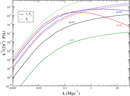
Figure 1: Left panel: total background ionised fraction as a function of redshift used. The right panel shows the power spectra for $x_{\mathrm{e}}\delta_{x_{\mathrm{e}}}$ as modelled in our analysis at different redshifts (thick solid). For comparison, we have also represented the power spectra for the baryon overdensity (dashed thin curves), which steadily grows in the late Universe.

As an illustration, we have represented in figure 1 the evolution of $x_{\mathrm{e}}(\eta)$, $x_{\mathrm{e}}^{2}P_{\delta_{x_{\mathrm{e}}}}(\eta,k)$ and $P_{\delta_{\mathrm{b}}}(\eta,k)$ at different times during the EoR for the currently favoured $\Lambda\textrm{CDM}$ model by the Planck satellite collaboration [63, 64].

4 Results

As above-mentioned, all the $\Lambda\textrm{CDM}$ cosmological parameters have been fixed to their currently favoured values by the Planck satellite collaboration [63, 64], and we have only considered primordial scalar perturbations. We have used the Song code to compute the late Universe collisional sources.

At second-order in perturbation theory we may compute the sources in isolation when studying individual perturbations $\Delta^{(2)}_{Xlm}$. However, when computing power spectra, correlations between the different effects may become relevant. This is the case for the various parts of the collision terms, and more generally, also between collision sources and other secondaries. For this reason, we have fully included the correlations between the gain and pure terms and, separately, the correlations within the loss terms. However, correlations with non-collisional secondaries, and between the gain and loss term, have been neglected so far.

Let us notice that, in principle, the power spectra are given by a genuine second-order perturbation (2$\times$2) and the correlation of a linear perturbation with a third order one (1$\times$3). Third order perturbations are beyond the scope of the Song code and cannot be straightforwardly computed. However, we expect the (2$\times$2) part to dominate the power spectra for the following reasons. For some effects, such as the kSZ or DOP for example, the second-order perturbations introduce new structures that are enhanced compared to the linear order. If the related third-order terms are not further enhanced compared to the already large second order ones, we find that $(\textrm{2$\times$2})\gg(\textrm{1$\times$3})$. See also the related discussion based on geometrical considerations in Ref. [35]. On the other hand, for the blurring effects, the potentially dominant third-order terms would be multiple blurring events along the line-of-sight, generated by the same structures that already exist at second order. We have been able to include these higher order contributions by performing multiple applications of the blurring potential, which is equivalent to what is performed in the more usual lensing computation (see section. 3.3.1).

Finally, let us stress that for the most interesting $B$-mode polarisation calculations, the linear part vanishes and the (1$\times$3) part is thus completely absent. Our derivation of the $B$-mode power spectrum is therefore exact.

4.1 Loss terms

In the literature the EoR loss term has been discussed in details, while we provide an unified approach further including the bSZ, bGR and bDOP effects. We first summarise our results for the blurring potential, followed by the calculation of the induced non-linear power spectra.

4.1.1 Blurring potential

The loss terms are accounted for by the blurring potential, which has been represented in figure 2, separated into its diverse components. As can be checked on this figure, the relativistic (bGR) and second order phase space enhancements (bDOP) effects have a negligible impact on $\kappa_{\mathrm{blur}}$, which is entirely dominated by the blurring Sunyaev-Zel’dovich and blurring reionisation effects, bSZ and bEoR, respectively.

This is expected for the relativistic blurring, bGR, sourced by the lapse function $A$ that is much smaller than the late Universe baryon densities responsible for the bSZ effect. The bDOP depends on the orientation of the velocity and tends to cancel along the line-of-sight, at least on the larger scales studied in this work. Concerning the bEoR contribution, as can be seen in figure 1, $\delta_{x_{\mathrm{e}}}$ can become larger than the baryon overdensity at EoR, but vanishes later on. After integrating along the line-of-sight, we find that bSZ and bEoR are comparable in amplitude. Only on the largest length scales the contribution from reionisation appears to be suppressed with respect to bSZ and this can be explained by the power streaming to smaller multipoles after the EoR.

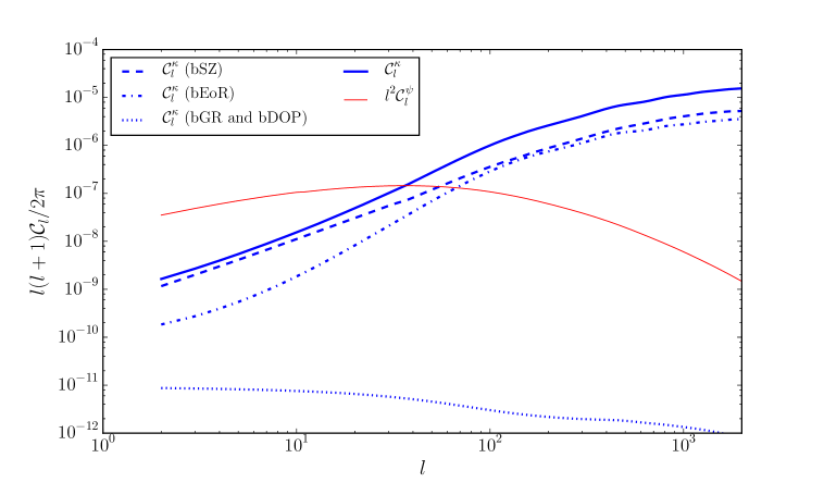
Figure 2: Angular power spectrum $\mathcal{C}_{l}^{\kappa}$ of the blurring potential $\kappa_{\mathrm{blur}}$ in blue together with its main components. For comparison, we have represented the lensing power spectrum $\mathcal{C}_{l}^{\Psi}$, multiplied by $l^{2}$. It should be noted that the lensing does act on the derivatives of the linear perturbations while the optical depth acts on the perturbations themselves and an absolute comparison cannot be drawn from this plot.

As previously mentioned, the bEoR contribution has been studied in some details in Ref. [26]. Our result shows that it is a good approximation to not include the bGR and bDOP contributions. In addition, we find that the bSZ and bEoR effects are about $50\%$ correlated. The reason is that the physics of reionisation is directly linked to the baryon over-densities, which are also responsible for the bSZ effect. A separate analysis of the bSZ and bEoR contributions would find the total blurring power spectrum significantly smaller.

The angular power spectrum of the blurring potential is almost featureless (blue solid curve in figure 2). All existing structures in the baryon overdensities, such as the baryon acoustic oscillations, are smoothed out by the integration along the line-of-sight.

Whereas the lensing potential is peaked at scales around $l\simeq 10$ to $100$, we find the blurring potential to have support up to much smaller scales. Lensing does locally distort the linear CMB fluctuations according to the large scale gravitational potentials, while blurring represents a reduction of power from regions where collisions out of the line-of-sight are more likely, tracing the distribution of matter in the Universe. This imprints a small scale signature onto the already inhomogeneous incoming CMB leading to a rise of power on the very small scales. As a consequence, the blurring must eventually dominate over lensing in the damping tail where the primary CMB does not posses much power.

4.1.2 Blurring induced CMB anisotropies

As discussed in section 2.3.3, we have integrated equations (3.16) to compute the temperature and $B$-mode angular power spectra induced by the blurring effects. They have been represented in figure 3.

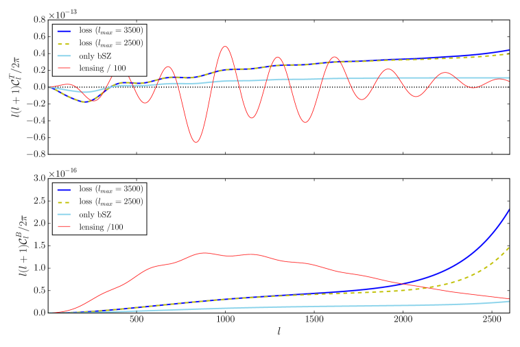
Figure 3: The blurring temperature ($\mathcal{C}_{l}^{T})$ and $B$-mode ($\mathcal{C}_{l}^{B}$) angular power spectra. The light blue line shows the bSZ effect in isolation. It has to be compared to the entire blurring spectrum (dark blue curve). Correlations cannot be neglected, in particular between bSZ and bEoR. We have also represented the lensing power spectra (divided by a factor $100$) in red. The blurring effects appear to be relatively enhanced on the smaller scales while the lensing becomes suppressed. This plot also shows the impact of the multipole moment cuts, either at $l=3500$ or $l=2500$.

Let us notice that all signatures of the linear spectra are washed out and the spectra extends far into the Silk damping tail. As previously mentioned, this is due to the support of $\kappa_{\mathrm{blur}}$ on the small scales. The light blue curve in figure 3 represents the angular spectra obtained by considering only the bSZ contribution, while the dark blue line includes all blurring contributions. As we have already seen in the blurring potential, the bSZ and bEoR effects are of comparable magnitude and strongly correlated.

For the temperature power spectra, the blurring effects are comparable in amplitude to one percent of the lensing up to $l\simeq 2000$. Let us notice that the lensing and blurring effects are possibly strongly correlated as they are sourced by the same density fields. The only difference is that the lensing depends, via the potential, on the inverse Laplacian of the density. Such a correlation might affect the lensing up to the $10\%$ level, especially towards the smaller scales and could potentially be responsible of some of the Planck lensing anomalies [65]. As previously discussed, we have kept the collision term in isolation and cannot currently compute this effect. We leave a combined lensing and blurring analysis for a future work.

Since we only perform the analysis to second order, we test the dependence of our results on the small scales by cutting the integration of Eq. (3.16) at $l=2500$ instead of $l=3500$. The temperature power spectrum is relatively stable under this cut, which suggests that our analysis should not be affected by unaccounted small scale non-linear physics beyond second order.

In addition to modifying the intensity, the blurring terms also generate polarisation. By locally reducing the linear $E$-modes due to collisions out of the line-of-sight, the blurring induces a mix of $E$- and $B$-modes. The $B$-mode angular power spectrum has been represented in the lower panel of figure 3. As for the temperature, the blurring $B$-modes spectrum is almost featureless and comparable to a percent of the lensing generated $B$-modes. Interestingly, $B$-modes are more significantly affected by non-linear corrections, as visible deviations appear by changing the multipole cut around $l=1500$. This is caused by the lack of large scale power in the linear $E$-mode polarisation, enhancing the signal’s dependence on the smaller scales. Again, unaccounted correlations between lensing and blurring $B$-modes might contaminate the $B$-modes after lensing has been cleaned and we let their derivation for a future work.

4.2 Pure and Gain terms

The pure and gain terms can be evaluated with the Song code (see sections 2.3.1 and 2.3.2). Up to our knowledge, the computation of the pure terms has not been performed so far and we find that they remain always negligible compared to the much larger gain terms, typically by at least two orders of magnitude. As long as the perturbative approach is applicable, the second-order perturbations remain smaller than their linear counterparts, at least when the later are not vanishing. This also holds for the growing baryon perturbations. The pure terms have the same structure as the linear collision ones and are therefore bound to be perturbatively small, provided we remain focused on the large and mildly non-linear scales.

For the first time we provide a full analysis of all second order gain sources. While many of the gain terms are comparable in amplitude to the pure terms, a few are significantly larger and dominate the signal. For the intensity these are the kSZ and the kEoR effects. Polarisation is not directly induced by the kSZ effect and various other contributions then become relevant. We find the polarisation gain terms to be driven by the pSZ, pDOP and pEoR effects. As one could have intuitively guessed, the dominant sources end up being the ones that contain the maximum number of baryon perturbations.

4.2.1 Accuracy tests

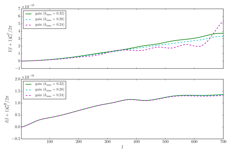
Figure 4: Accuracy tests for the gain terms angular power spectra associated with a truncation of the Fourier decomposition at different wavenumber values $k_{\max}$ (in $\mathrm{Mpc}^{-1}$). Since Song is a second-order perturbation code, the fully non-linear corrections expected at small scales are not accounted for and one can trust the numerical results only when these ones decouple from the small scale modes. We find that multipoles larger than $l=500$ already receive significant power from the small scale modes and are beyond the capabilities of a second-order perturbative analysis. It should be noted that we have optimised our numerical parameters for the range $l<500$ and the output cannot be trusted on smaller scales.

In Fig. 4, we analyse how much power is transferred from the very small and non-linear scales into our large scale angular power spectra by cutting the Fourier integrations at a given wavenumber $k_{\max}$.

For the temperature (upper panel), rather small multipoles, of the order $l\simeq 500$, appear to be already affected by small scale physics. This comes from the kSZ effect, which is given by a convolution over the baryon density contrast and velocity perturbations. Both are present over the entire range of scales but gravitational instability make them of larger amplitude at the smaller scales. When evaluating the convolution product at large scales, the small scale modes do contribute significantly and physically describe the transfer of power from two small scale modes into a large scale perturbation. We conclude that a second-order code is not suitable to compute kSZ and kEoR effects for multipoles larger than $l\gtrsim 500$, where non-linear corrections become relevant. Our result can therefore be trusted for $l<500$.

As can be seen in the $B$-mode power spectrum in figure 4, for polarisation, the situation is improved and non-linearities are not expected to play a significant role up to $l=700$. Contributing to polarisation, the pSZ and pEoR effects, depend on the linear photon quadrupoles, and consequently one Fourier mode is evaluated at very large scales. Even though the baryon density is then evaluated at a smaller scale, the transfer of power from small scales into large scales is suppressed. However, polarisation is also generated by the phase space enhancement terms (pDOP), which involve the baryon velocities squared and allow a transfer of power similar to the kSZ terms.

4.2.2 Gain induced CMB anisotropies

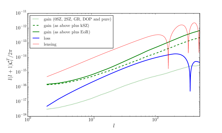
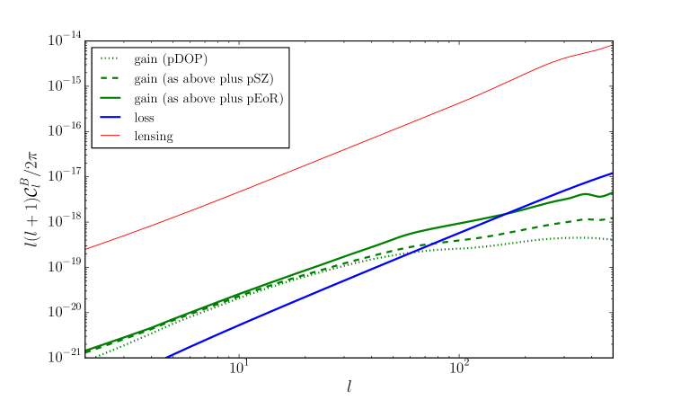
Figure 5: Temperature (upper panel) and $B$-mode (lower panel) angular power spectrum for the gain terms, separated into their main components. For comparison, the blurring (loss terms) and lensing have been reported. For temperature, the signal is dominated by the kSZ and kEoR effects, while the relativistic (GR), pure and phase space enhancement (DOP) contributions remain two orders of magnitude smaller. For polarisation, the large scales are dominated by the pDOP effect, while on smaller scales the pSZ and pEoR effects become relevant. The signal is comparable in size to the loss contributions.

The temperature angular power spectrum $l(l+1)\mathcal{C}_{l}^{T}/(2\pi)$ generated by the gain and pure terms has been represented in the upper panel of figure 5. We find that the contributions due to the relativistic (GR), phase space enhancement (DOP) and pure terms are subleading, and the signal is essentially made up of the kSZ and kEoR effects [48, 49, 51, 50]. The kEoR is smaller than the kSZ on very large scales as it tends to be erased during the post EoR period. As for the blurring, we find a strong correlation between kSZ and kEoR increasing their combined power spectrum. Overall, the gain contribution for the temperature power spectrum is about one order of magnitude larger than the blurring. It remains smaller than the lensing over the entire range of analysed scales, but not by much. It is possible that correlations between the gain and loss terms, or the gain and lensing terms are important and these have not been considered here.

The lower panel of figure 5 shows the induced $B$-mode angular power spectrum $l(l+1)\mathcal{C}_{l}^{B}/(2\pi)$ induced by the gain terms. In addition to the pSZ and pEoR effects, which have been studied in isolation in Refs. [34, 47, 28], we have been able to compute for the first time the pGR, pDOP and pure contributions together with their correlations. As opposed to the temperature power spectra, which are dominated by the kSZ and kEoR effects, we find the pDOP contributions to be important for the $B$-modes, where they actually dominate the signal on the large scales. This can be understood by remarking that, contrary to the pSZ effect, the pDOP terms can transfer power from the small scales to the large scales. In parallel, the pSZ and pEoR effects become more important on the smaller scales and are, again, strongly correlated.

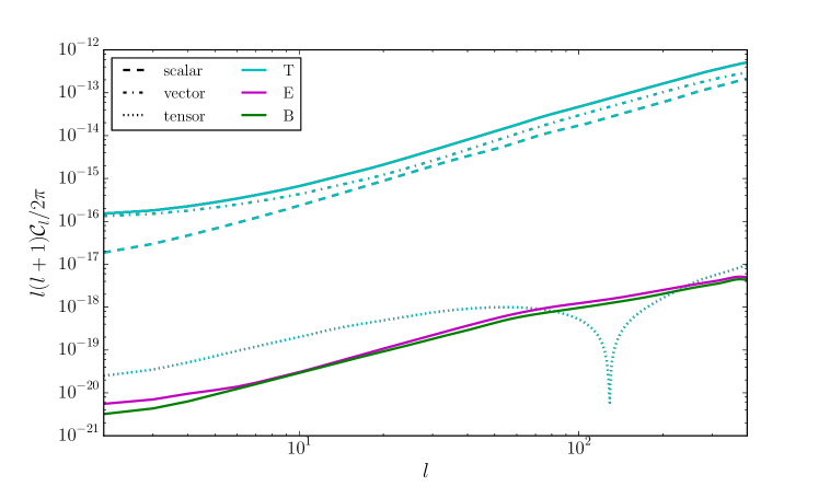
Figure 6: Temperature and polarisation spectra induced from the collisional gain terms. The scalar, vector and tensor contributions of $\mathcal{C}_{l}^{T}$ are represented. Temperature dominates over polarisation due to the kSZ and kEoR effects, which are able to generate scalar and vector modes only. The much smaller tensor modes are however comparable to both $E$ and $B$ polarisation which mix in free streaming.

Figure 6 finally shows the temperature, $E$- and $B$-mode angular power spectra induced by the gain terms and we have separated $\mathcal{C}_{l}^{T}$ into its scalar ($m=0$), vector ($m=\pm 1$) and tensor ($m=\pm 2$) contributions. The dominant kSZ and kEoR effects driving $\mathcal{C}_{l}^{T}$ only induce scalars and vectors, while the tensors are sourced by the subleading 2SZ and DOP terms. Polarisation is also not induced from the kSZ and kEoR effects, which explains why $\mathcal{C}_{l}^{E}$ and $\mathcal{C}_{l}^{B}$ are of similar magnitude as the temperature’s tensors. The $E$- and $B$-modes mix in free-streaming and consequently have a similar shape and amplitude. This is reason why we have not represented the $E$-mode signal in the previous plots. Only on very large scales, one can see that $\mathcal{C}_{l}^{B}$ is slightly lower than $\mathcal{C}_{l}^{E}$. On these scales, there is indeed not enough time after EoR to convert all of the induced $E$-mode polarisation into $B$-modes.

4.3 Combined result of collisional secondaries

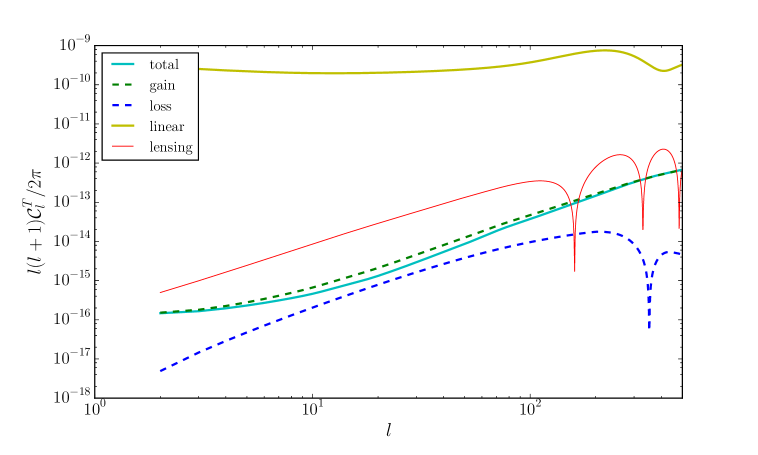
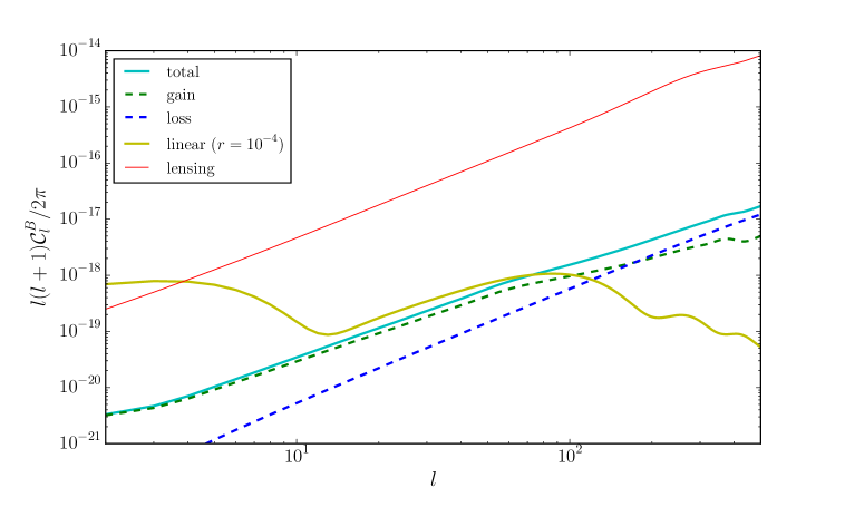
Figure 7: Temperature (upper panel) and $B$-mode (lower panel) angular power spectra induced by all terms. For comparison, we have represented the lensing power spectra as well as primordial $B$-modes that would be generated by a tensor-to-scalar ratio $r=10^{-4}$. For temperature, $C_{l}^{T}$ remains smaller than lensing but only by a factor of a few. For polarisation, the induced $B$-modes remain always smaller than lensing but match the primordial ones all over the range $l\in[10,100]$.

In figure 7, we have summarized our results and plotted the total temperature and $B$-mode polarisation angular power spectra for all collisional secondaries. For comparison, the lensing induced signals and the primordial $B$-modes associated with a tensor-to-scalar ratio of $r=10^{-4}$ have been represented. The temperature power spectrum $\mathcal{C}_{l}^{T}$ is essentially driven by the gain contributions on all scales and remains smaller than lensing, but only by a factor of a few. The polarisation spectra $\mathcal{C}_{l}^{E}$ and $\mathcal{C}_{l}^{B}$ are always of comparable amplitude due to their mixing by free streaming and we have represented only $\mathcal{C}_{l}^{B}$. They are sourced by the gain terms on large scales and by the blurring on small scales. On all the multipole range studied, the polarisation power spectra remain much smaller than the lensing induced ones.

Let us stress however that the $B$-mode signal we have computed is of comparable amplitude to the primordial one induced by a tensor-to-scalar ratio of $r=\mathcal{O}\!\left(10^{-4}\right)$, all over the range $l=10$ to $100$. Various experiments have been proposed to target very small tensor-to-scalar ratios [1, 66], and they would rely on our ability to perform delensing on the foreground-cleaned $B$-modes [67, 68, 69, 70]. Our result shows that, from $l=10$ to $100$, all of the late Universe diffuse secondaries are important, and especially the pDOP contribution. Interestingly, it remains a clean window for primordial $B$-modes on the very large scales, $l<10$, favouring the case for full sky experiments [71, 6, 72].

Finally, as already mentioned, the $B$-modes presented in our plots are not subject to (1$\times$3) terms and the approximation of including all possible contributions up to second order is very accurate on the large scales; fully non-linear corrections eventually appearing for $l\gtrsim 800$. Nevertheless, some uncertainties remain from the physics of reionisation and the currently neglected correlations between gain, loss and lensing, which will be investigated in a future work.

5 Conclusions

We have employed the second-order Boltzmann code Song to obtain an unified framework to compute the CMB anisotropies induced by late-time collisional secondaries. These were the last missing pieces of a complete second order Boltzmann treatment of the cosmological perturbations [23]. Our results show that the collisional sources in the late Universe are significantly larger than the second order recombination effects already implemented in Song and studied in Refs. [37, 23]. While the likelihood for a CMB photon to have an interaction in the late Universe is much smaller than the chance of having last scattered at recombination, the imprint in the CMB is nevertheless enhanced. This is due to the baryon perturbations, which grow during the evolution of the Universe and are much larger at reionisation compared to recombination.

For the first time, we have included all collisional secondaries in a relativistic non-linear Boltzmann code. Our sources include the diffuse versions of the Sunyaev-Zel’dovich effect for the temperature and polarisation, the impact of patchy reionisation, but also the blurring Sunyaev-Zel’dovich. Our framework naturally encompasses a range of novel relativistic and pure second order effects, plus some phase space enhancement terms which have only been discussed for temperature in Ref. [35].

Among these novel contributions, the pure terms are structurally very complex as they include non-linear effects from the evolution of the Universe before the EoR. However, we have found that they are of the expected size for second-order perturbative effects and thus remain subleading compared to the others. The same holds for the relativistic corrections, labelled as bGR, 0GR, 2GR and pGR, that depend on the gravitational potentials. We further show that the polarised phase space enhancement terms, referred to as pDOP, are relevant and even dominate the large scale B-mode polarisation power spectrum.

The kinetic and blurring Sunyaev-Zel’dovich and reionisation effects describe the inhomogeneously increased likelihood of collisions in overdense regions and due to patchy reionisation. While the kSZ, kEoR and bEoR effects are well-known in the literature (see section 1), we also compute the polarised blurring and find that it provides a significant contribution to the induced $B$-mode polarisation.

Reionisation and SZ effects are often discussed in isolation. Having both effects implemented in the Song code allows us to study their correlations. The SZ and EoR contributions have been shown to be strongly correlated, by no less than $50\%$, which significantly affects the resulting power spectra compared to a separate analysis.

Due to the similarities between lensing and blurring that we have pointed out, one may expect a comparable correlation between the lensing and blurring effects. We have found that the blurring is typically comparable to a percent of the lensing signal but correlations could possibly be as large as $10\%$ of the lensing signal. These ones have however not been computed and will be pursued in a future work.

In summary, we have shown that the $B$-modes generated at, and after, EoR, including the novel effects discussed above, are of the same amplitude than the primordial ones stemming from a tensor-to-scalar ratio of $r=10^{-4}$ over a large range of scales. They may become relevant in future CMB experiments. Potential correlations of these with the lensing $B$-modes might further enhance the signal.

Concerning the numerics, we have tested the impact of the non-resolved small scale perturbations in Song on the larger scale power spectra and find that our accuracy is maintained up to $l\simeq 500$ for the gain sources, while the blurring is accurate up to $l\simeq 1500$. The ability to compute all late Universe collisional secondaries will be soon added to the publicly available Song code [19]. In the meanwhile the code is available upon request.

References

- [1] T. Matsumura et al., Mission design of LiteBIRD, 1311.2847.
- [2] Planck collaboration, R. Adam et al., Planck intermediate results. XLVII. Planck constraints on reionization history, Astron. Astrophys. 596 (2016) A108, [1605.03507].
- [3] CORE Collaboration, F. Finelli, M. Bucher, A. Achúcarro, M. Ballardini, N. Bartolo et al., Exploring Cosmic Origins with CORE: Inflation, ArXiv e-prints (Dec., 2016) , [1612.08270].
- [4] Planck collaboration, N. Aghanim et al., Planck intermediate results. LIII. Detection of velocity dispersion from the kinetic Sunyaev-Zeldovich effect, 1707.00132.
- [5] M. Remazeilles, A. J. Banday, C. Baccigalupi, S. Basak, A. Bonaldi, G. De Zotti et al., Exploring Cosmic Origins with CORE: B-mode Component Separation, ArXiv e-prints (Apr., 2017) , [1704.04501].
- [6] J. Delabrouille, P. de Bernardis, F. R. Bouchet, A. Achúcarro, P. A. R. Ade, R. Allison et al., Exploring Cosmic Origins with CORE: Survey requirements and mission design, ArXiv e-prints (June, 2017) , [1706.04516].
- [7] A.-S. Deutsch, E. Dimastrogiovanni, M. C. Johnson, M. Münchmeyer and A. Terrana, Reconstruction of the remote dipole and quadrupole fields from the kinetic Sunyaev Zel’dovich and polarized Sunyaev Zel’dovich effects, 1707.08129.
- [8] A. Lewis, A. Challinor and A. Lasenby, Efficient computation of CMB anisotropies in closed FRW models, Astrophys. J. 538 (2000) 473–476, [astro-ph/9911177].
- [9] J. Lesgourgues, The Cosmic Linear Anisotropy Solving System (CLASS) I: Overview, ArXiv e-prints (Apr., 2011) , [1104.2932].
- [10] D. Blas, J. Lesgourgues and T. Tram, The Cosmic Linear Anisotropy Solving System (CLASS) II: Approximation schemes, JCAP 1107 (2011) 034, [1104.2933].
- [11] M. J. Rees and D. W. Sciama, Large-scale density inhomogeneities in the universe, Nature 217 (1968) 511–516.
- [12] U. Seljak, Rees-Sciama effect in a CDM universe, Astrophys. J. 460 (1996) 549, [astro-ph/9506048].
- [13] A. Cooray, Nonlinear integrated Sachs-Wolfe effect, Phys. Rev. D65 (2002) 083518, [astro-ph/0109162].
- [14] A. Blanchard and J. Schneider, Gravitational lensing effect on the fluctuations of the cosmic background radiation, Astronomy and Astrophysics 184 (1987) 1–6.
- [15] A. Kashlinsky, Small-scale fluctuations in the microwave background radiation and multiple gravitational lensing, The Astrophysical Journal 331 (1988) L1–L4.
- [16] A. Lewis and A. Challinor, Weak gravitational lensing of the cmb, Phys. Rept. 429 (2006) 1–65, [astro-ph/0601594].
- [17] U. Seljak, Large scale structure effects on the gravitational lens image positions and time delay, Astrophys. J. 436 (1994) 509–516, [astro-ph/9405002].
- [18] Z. Huang and F. Vernizzi, Cosmic Microwave Background Bispectrum from Recombination, Phys. Rev. Lett. 110 (2013) 101303, [1212.3573].
- [19] G. W. Pettinari, C. Fidler, R. Crittenden, K. Koyama and D. Wands, The intrinsic bispectrum of the Cosmic Microwave Background, JCAP 1304 (2013) 003, [1302.0832].
- [20] C. Fidler, K. Koyama and G. W. Pettinari, A new line-of-sight approach to the non-linear Cosmic Microwave Background, JCAP 1504 (2015) 037, [1409.2461].
- [21] R. Saito, A. Naruko, T. Hiramatsu and M. Sasaki, Geodesic curve-of-sight formulae for the cosmic microwave background: a unified treatment of redshift, time delay, and lensing, Journal of Cosmology and Astroparticle Physics 2014 (2014) 051.
- [22] S. C. Su, E. A. Lim and E. P. S. Shellard, CMB Bispectrum from Non-linear Effects during Recombination, 1212.6968.
- [23] G. W. Pettinari, C. Fidler, R. Crittenden, K. Koyama, A. Lewis and D. Wands, Impact of polarization on the intrinsic cosmic microwave background bispectrum, Phys. Rev. D90 (2014) 103010, [1406.2981].
- [24] A. Loeb and R. Barkana, The Reionization of the Universe by the First Stars and Quasars, Ann. Rev. Astron. Astrophys. 39 (2001) 19–66, [astro-ph/0010467].
- [25] R. Barkana and A. Loeb, The Physics and Early History of the Intergalactic Medium, Rept. Prog. Phys. 70 (2007) 627, [astro-ph/0611541].
- [26] C. Dvorkin and K. M. Smith, Reconstructing Patchy Reionization from the Cosmic Microwave Background, Phys. Rev. D79 (2009) 043003, [0812.1566].
- [27] W. Hu, Reionization revisited: secondary cmb anisotropies and polarization, Astrophys. J. 529 (2000) 12, [astro-ph/9907103].
- [28] O. Dore, G. Holder, M. Alvarez, I. T. Iliev, G. Mellema, U.-L. Pen et al., The Signature of Patchy Reionization in the Polarization Anisotropy of the CMB, Phys. Rev. D76 (2007) 043002, [astro-ph/0701784].
- [29] K. M. Smith and S. Ferraro, Detecting Patchy Reionization in the Cosmic Microwave Background, Phys. Rev. Lett. 119 (2017) 021301, [1607.01769].
- [30] C. Hernandez-Monteagudo and R. A. Sunyaev, Galaxy Clusters as mirrors of the distant Universe. Implications for the kSZ and ISW effects, Astron. Astrophys. 509 (2010) A82, [0905.3001].
- [31] R. A. Sunyaev and I. B. Zeldovich, The velocity of clusters of galaxies relative to the microwave background - The possibility of its measurement, Mon. Not. R. Astron. Soc. 190 (Feb., 1980) 413–420.
- [32] J. P. Ostriker and E. T. Vishniac, Generation of microwave background fluctuations from nonlinear perturbations at the ERA of galaxy formation, Astrophys. J.Lett. 306 (July, 1986) L51–L54.
- [33] A. H. Jaffe and M. Kamionkowski, Calculation of the Ostriker-Vishniac effect in cold dark matter models, Phys. Rev. D58 (1998) 043001, [astro-ph/9801022].
- [34] S. Y. Sazonov and R. A. Sunyaev, Microwave polarization in the direction of galaxy clusters induced by the CMB quadrupole anisotropy, Mon. Not. Roy. Astron. Soc. 310 (1999) 765–772, [astro-ph/9903287].
- [35] W. Hu, D. Scott and J. Silk, Reionization and cosmic microwave background distortions: A Complete treatment of second order Compton scattering, Phys. Rev. D49 (1994) 648–670, [astro-ph/9305038].
- [36] M. Beneke and C. Fidler, Boltzmann hierarchy for the cosmic microwave background at second order including photon polarization, Phys. Rev. D82 (2010) 063509, [1003.1834].
- [37] M. Beneke, C. Fidler and K. Klingmuller, B polarization of cosmic background radiation from second-order scattering sources, JCAP 1104 (2011) 008, [1102.1524].
- [38] U. Seljak and M. Zaldarriaga, A line of sight approach to cosmic microwave background anisotropies, Astrophys. J. 469 (1996) 437–444, [astro-ph/9603033].
- [39] W. Hu and M. J. White, CMB anisotropies: Total angular momentum method, Phys. Rev. D56 (1997) 596–615, [astro-ph/9702170].
- [40] C. Pitrou, The Radiative transfer at second order: A Full treatment of the Boltzmann equation with polarization, Class. Quant. Grav. 26 (2009) 065006, [0809.3036].
- [41] S. Yasini and E. Pierpaoli, Kinetic Sunyaev Zeldovich effect in an anisotropic CMB model: measuring low multipoles of the CMB at higher redshifts using intensity and polarization spectral distortions, Phys. Rev. D94 (2016) 023513, [1605.02111].
- [42] E. T. Vishniac, Reionization and small-scale fluctuations in the microwave background, Astrophys. J. 322 (Nov., 1987) 597–604.
- [43] A. Challinor, M. Ford and A. Lasenby, Thermal and kinematic corrections to the microwave background polarization induced by galaxy clusters along the line of sight, Mon. Not. Roy. Astron. Soc. 312 (2000) 159–165, [astro-ph/9905227].
- [44] A. R. Cooray and D. Baumann, CMB polarization towards clusters as a probe of the integrated Sachs-Wolfe effect, Phys. Rev. D67 (2003) 063505, [astro-ph/0211095].
- [45] E. F. Bunn, Probing the universe on gigaparsec scales with remote cosmic microwave background quadrupole measurements, Phys. Rev. D73 (2006) 123517, [astro-ph/0603271].
- [46] A. Hall and A. Challinor, Detecting the polarization induced by scattering of the microwave background quadrupole in galaxy clusters, Phys. Rev. D90 (2014) 063518, [1407.5135].
- [47] M. G. Santos, A. Cooray, Z. Haiman, L. Knox and C.-P. Ma, Small-Scale Cosmic Microwave Background Temperature and Polarization Anisotropies Due to Patchy Reionization, Astrophys. J. 598 (Dec., 2003) 756–766, [arXiv:astro-ph/0305471].
- [48] M. McQuinn, S. R. Furlanetto, L. Hernquist, O. Zahn and M. Zaldarriaga, The Kinetic Sunyaev-Zel’dovich effect from reionization, Astrophys. J. 630 (2005) 643–656, [astro-ph/0504189].
- [49] I. T. Iliev, U.-L. Pen, J. R. Bond, G. Mellema and P. R. Shapiro, The Kinetic Sunyaev-Zel’dovich Effect from Radiative Transfer Simulations of Patchy Reionization, Astrophys. J. 660 (2007) 933–944, [astro-ph/0609592].
- [50] H. Park, P. R. Shapiro, E. Komatsu, I. T. Iliev, K. Ahn and G. Mellema, The Kinetic Sunyaev-Zel’dovich effect as a probe of the physics of cosmic reionization: the effect of self-regulated reionization, Astrophys. J. 769 (2013) 93, [1301.3607].
- [51] M. A. Alvarez, The Kinetic Sunyaev–Zel’dovich Effect From Reionization: Simulated Full-sky Maps at Arcminute Resolution, Astrophys. J. 824 (2016) 118, [1511.02846].
- [52] M. Bartelmann and P. Schneider, Weak gravitational lensing, Phys. Rept. 340 (2001) 291–472, [astro-ph/9912508].
- [53] M. McQuinn, L. Hernquist, M. Zaldarriaga and S. Dutta, Studying Reionization with Ly-alpha Emitters, Mon.Not.Roy.Astron.Soc. 381 (2007) 75–96, [0704.2239].
- [54] O. Zahn, A. Lidz, M. McQuinn, S. Dutta, L. Hernquist, M. Zaldarriaga et al., Simulations and Analytic Calculations of Bubble Growth During Hydrogen Reionization, Astrophys. J. 654 (2006) 12–26, [astro-ph/0604177].
- [55] V. Jelic et al., Foreground simulations for the LOFAR - Epoch of Reionization Experiment, Mon.Not.Roy.Astron.Soc. 389 (2008) 1319–1335, [0804.1130].
- [56] O. Zahn, A. Mesinger, M. McQuinn, H. Trac, R. Cen and L. E. Hernquist, Comparison Of Reionization Models: Radiative Transfer Simulations And Approximate, Semi-Numeric Models, Mon. Not. Roy. Astron. Soc. 414 (2011) 727, [1003.3455].
- [57] I. T. Iliev, M. G. Santos, A. Mesinger, S. Majumdar and G. Mellema, Epoch of Reionization modelling and simulations for SKA, PoS AASKA14 (2015) 007, [1501.04213].
- [58] Y. Lin, S. P. Oh, S. R. Furlanetto and P. M. Sutter, The Distribution of Bubble Sizes During Reionization, Mon. Not. Roy. Astron. Soc. 461 (2016) 3361–3374, [1511.01506].
- [59] A. Bauer, V. Springel, M. Vogelsberger, S. Genel, P. Torrey, D. Sijacki et al., Hydrogen Reionization in the Illustris universe, Mon. Not. Roy. Astron. Soc. 453 (2015) 3593–3610, [1503.00734].
- [60] Y. Mao, M. Tegmark, M. McQuinn, M. Zaldarriaga and O. Zahn, How accurately can 21 cm tomography constrain cosmology?, Phys. Rev. D78 (2008) 023529, [0802.1710].
- [61] S. Clesse, L. Lopez-Honorez, C. Ringeval, H. Tashiro and M. H. G. Tytgat, Background reionization history from omniscopes, Phys. Rev. D86 (2012) 123506, [1208.4277].
- [62] A. Lewis, Cosmological parameters from WMAP 5-year temperature maps, Phys. Rev. D78 (2008) 023002, [0804.3865].
- [63] Planck collaboration, P. A. R. Ade et al., Planck 2013 results. XVI. Cosmological parameters, Astron. Astrophys. 571 (2014) A16, [1303.5076].
- [64] Planck collaboration, D. Paoletti, Planck 2015 Cosmological Results, in Proceedings, Magellan Workshop: Connecting Neutrino Physics and Astronomy: Hamburg, Germany, March 17-18, 2016, pp. 71–86, 2016. DOI.
- [65] Planck collaboration, P. A. R. Ade et al., Planck 2015 results. XV. Gravitational lensing, Astron. Astrophys. 594 (2016) A15, [1502.01591].
- [66] CMB-S4 collaboration, K. N. Abazajian et al., CMB-S4 Science Book, First Edition, 1610.02743.
- [67] K. M. Smith, D. Hanson, M. LoVerde, C. M. Hirata and O. Zahn, Delensing CMB Polarization with External Datasets, JCAP 1206 (2012) 014, [1010.0048].
- [68] J. Errard, S. M. Feeney, H. V. Peiris and A. H. Jaffe, Robust forecasts on fundamental physics from the foreground-obscured, gravitationally-lensed CMB polarization, JCAP 1603 (2016) 052, [1509.06770].
- [69] J. Carron, A. Lewis and A. Challinor, Internal delensing of Planck CMB temperature and polarization, JCAP 1705 (2017) 035, [1701.01712].
- [70] M. Millea, E. Anderes and B. D. Wandelt, Bayesian delensing of CMB temperature and polarization, 1708.06753.
- [71] H. Ishino, LiteBIRD, Int. J. Mod. Phys. Conf. Ser. 43 (2016) 1660192.
- [72] CMB-S4 collaboration, M. H. Abitbol et al., CMB-S4 Technology Book, First Edition, 1706.02464.