The response of the terrestrial bow shock and magnetopause to the long term decline in solar polar fields

Abstract

The location of the terrestrial magnetopause (MP) and it’s subsolar stand-off distance depends not only on the solar wind dynamic pressure and the interplanetary magnetic field (IMF), both of which play a crucial role in determining it’s shape, but also on the nature of the processes involved in the interaction between the solar wind and the magnetosphere. The stand-off distance of the earth’s MP and bow shock (BS) also define the extent of terrestrial magnetic fields into near-earth space on the sunward side and have important consequences for space weather. However, asymmetries due to the direction of the IMF are hard to account for, making it nearly impossible to favour any specific model over the other in estimating the extent of the MP or BS. Thus, both numerical and empirical models have been used and compared to estimate the BS and MP stand-off distances as well as the MP shape, in the period Jan. 1975$-$Dec. 2016, covering solar cycles 21–24. The computed MP and BS stand-off distances have been found to be increasing steadily over the past two decades, since $\sim$1995, spanning solar cycles 23 and 24. The increasing trend is consistent with earlier reported studies of a long term and steady decline in solar polar magnetic fields and solar wind micro-turbulence levels. The present study, thus, highlights the response of the terrestrial magnetosphere to the long term global changes in both solar and solar wind activity, through a detailed study of the extent and shape of the terrestrial MP and BS over the past four solar cycles, a period spanning the last four decades.

1 Introduction

It is well known that energetic events on the sun such as CMEs, flares, prominences, and high speed solar wind streams, gives rise to geomagnetic disturbances on the earth. Even during events known as solar wind disappearance events (Balasubramanian et al., 2003; Janardhan et al., 2005, 2008a, 2008b), when the earth was engulfed by the extremely low densities observed at 1 AU ($<$ 0.1 $\textrm{cm}^{-3}$) for periods exceeding 24 hours, the earth’s magnetosphere and the bow shock (BS) expanded dramatically. During the well known and studied 11 May 1999 disappearance event, it was estimated that the bow shock moved outward to distances beyond 45 earth radii (R_E) (Fairfield et al., 2001), compared to their normal value of $\sim$14 R_E. recent study (Rout et al., 2017) has shown that the lateral extent of the earth’s magnetopause (MP) plays a crucial role in determining the geoeffectiveness of solar wind outflows, with flows deviating by more than 6^∘ from the radial direction being non-geoeffective, as such flows will entirely miss the MP. Also, the BS and MP are essential in determining the behaviour of the magnetosheath, which plays a major role in the solar wind $-$ magnetosphere coupling (Lopez et al., 2011). The importance of the size and shape of the MP and BS cannot therefore be underestimated as they play a key role in space weather studies

It is known that the solar wind dynamic pressure and the IMF play a crucial role in determining the shape of the earth’s magnetosphere, which is basically parametrized by the position and the shape of the BS and MP. The BS forms in the upstream region of the magnetosphere, followed by the magnetosheath, bounded below by the MP. The extent of the BS and MP can be known by estimating stand-off distances of the BS and MP. McComas et al. (2013) calculated the canonical stand-off distance of the BS, which is about 11 earth radii (R_E), for the period 2009 to 2013, covering the minimum of cycle 23 to the early rise phase of cycle 24, compared to about 10 R_E for the period 1974 to 1994, covering cycles 21–22. These changes are in keeping with the observed decline in solar wind dynamic pressure from $\sim$2.4 nPa (1974$-$1994) to $\sim$1.4 nPa (2009$-$2013). The cycle 23 minimum in 2008$-$2009 experienced the slowest solar wind with the weakest solar wind dynamic pressure and IMF as compared to the earlier three cycles and observations by Ulysses, the out-of-ecliptic spacecraft which explored the mid and high latitude heliospheric solar wind, have also reported a significant global decrease in the solar wind dynamic pressure and in the IMF during the minimum of cycle 23, as compared to the minima of the earlier two cycles (Richardson et al., 2001; McComas et al., 2003; Jian et al., 2011). The changing shape of the MP and BS with time is therefore important in understanding space weather and in planetary exploration because much like the earth, other planetary magnetosphere would have also undergone changes in their MP shape as a result of the observed global reduction in solar wind dynamic pressure.

Equally, the long term variability in the solar magnetic fields can induce changes in the terrestrial magnetosphere, with the solar wind providing the complex link through which the effect is mediated. It is now well established that the near-earth space environment, at 1 AU, is strongly linked to the changes in the cyclic magnetic activity of the sun, driven essentially by the magnetic changes occurring in it’s interior. This link has been of particular interest to the solar and space science community due to the peculiar behavior seen in solar cycles 23 and 24 and in view of the long term changes taking place on the sun and in the solar wind (Janardhan et al., 2010, 2011; Bisoi et al., 2014a). The solar cycle 24, was preceded not only by one of the deepest minima in the past 100 years but the peak smoothed sunspot number (V2.0) was $\sim$116 in April 2014, making it the weakest sunspot cycle since cycle 14, which had a smoothed peak sunspot number (V2.0) of $\sim$107 in February 1906. It must be clarified here that as of July 2015 a revised and updated list of the (Wolf) sunspot numbers has been adopted, referred to as V2.0 (Clette & Lefèvre, 2016; Cliver, 2016). Also, the cycle 24 is the third successive cycle in a trend of diminishing sunspot cycles.

Our studies (Janardhan et al., 2011; Bisoi et al., 2014a; Janardhan et al., 2015) have shown a steady and continuous decline of solar high-latitude photospheric fields since mid-1990’s, and also in solar wind micro-tubulence levels in the inner heliosphere, spanning heliocentric distances from 0.2 to 0.8 AU (Bisoi et al., 2014b), in sync with photospheric magnetic fields. The long term declining trends seen in both photospheric magnetic fields and solar wind micro-turbulence levels over the entire inner-heliosphere, coupled with the unusually deep solar minimum in cycle 23 and the very unusual solar polar field conditions in cycle 24 (Gopalswamy et al., 2016), implies that these changes would directly affect the size and shape of the terrestrial magnetosphere. By estimating the variations in the stand-off distances of the BS and MP, one can actually quantify the effect of solar wind dynamic pressure and IMF on the earth’s magnetosphere and in turn link it to the solar cycle activity.

In the present paper, we have examined the solar wind dynamic pressure and the IMF at 1 AU over the last four decades, from 1975$-$2016 and estimated the stand-off distances of the BS and MP in order to study the behaviour of earth’s magnetosphere over time. In addition to the direct dependence of the stand-off distance on solar wind dynamic pressure, it has long been predicted and observed that the location and shape of the BS and MP depends on various solar wind conditions (Spreiter et al., 1966; Fairfield, 1971; Cairns & Lyon, 1995; Verigin et al., 1999; Fairfield et al., 2001). However, accurate theoretical as well as observational models for the BS and MP do not exist at present. We have therefore used both empirical and numerical models together to exploit this dependence and estimate the position of BS and MP as a function of time.

Earlier studies of sunspot activity reveal periods like the Maunder minimum (1645-1715) when the sunspot activity was extremely low or almost non-existent. Using records of ¹⁴C from tree rings over the past 1000 solar cycles or 11,000 years, (Usoskin et al., 2007) have identified 27 such prolonged or grand solar minima, each lasting on average $\sim$6–7 solar cycles. The recent observations of anomalies in solar cycle activity in solar cycle 23 and 24, as mentioned earlier, have caught the attention of many researchers who have predicted future solar cycle activity to be heading towards a Maunder minimum like situation (Zolotova & Ponyavin, 2014; Zachilas & Gkana, 2015; Sánchez-Sesma, 2016). From a study of decadal group sunspot number, a maximum group sunspot number of $\sim$60 was predicted Usoskin et al. (2014), just prior to the onset of the Maunder minimum. Another study (Janardhan et al., 2015), predicted a solar maximum for cycle 25, of 62$\pm$12 similar to conditions prior to the onset of the Maunder minimum. Recent reports have claimed that the sun may move into a period of very low sunspot activity comparable with the Dalton (Zolotova & Ponyavin, 2014) or even the Maunder minimum (Sánchez-Sesma, 2016; Zachilas & Gkana, 2015; Janardhan et al., 2015). It is therefore necessary to access the possible impact of such unusually low solar activity on the earth’s magnetosphere.

2 Observations

2.1 Solar photospheric magnetic fields

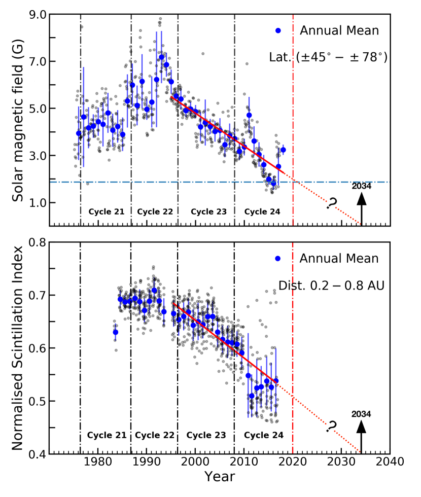
Figure 1: Photospheric magnetic fields in the latitude range $45^{\circ}-78^{\circ}$ for the period Feb1975$-$Dec2016 (upper panel) and solar wind micro-turbulence levels from 327 MHz IPS observations in the period 1983$-$2016 and in the distance range 0.2$-$0.8 AU (lower panel). The filled gray dots in both panels are actual measurements of magnetic fields (top) and solar wind micro-turbulence (bottom), while the filled blue circles are annual means shown with 1$\sigma$ error bars. The solid red line in both panels is a best fit to the declining trends for the annual means while the dotted red lines are extrapolations of the best fit until 2034 for the photospheric fields (top) and the IPS observations (bottom). The ’?’ and the horizontal light blue dot-dashed line at 1.8 G are explained in the text. The vertical red dashed line in both panels indicates the expected minimum of the current solar cycle 24 in 2020.

Solar activity has been steadily decreasing over the past two decades and Figure 1 shows the decline observed in both solar photospheric magnetic fields (upper panel) and solar wind micro-turbulence levels (lower panel). The upper panel uses observations for the period Feb.1975$-$Dec.2016 in the latitude range $45^{\circ}$-$78^{\circ}$. Magnetic fields were computed using synoptic magnetograms from the National Solar Observatory, Kitt Peak (NSO/KP), the Synoptic Optical Long-term Investigations of the Sun (NSO/SOLIS) facility and the Global Oscillation Network Group (GONG). Each synoptic magnetogram used, is available in standard FITS format and represents one Carrington rotation or 27.2753 day averaged photospheric magnetic fields in units of Gauss. Further details about the computation of magnetic fields can be referred to in Janardhan et al. (2010).

The filled grey dots in Fig.1 are actual measurements while the filled blue circles are annual means shown with 1$\sigma$ error bars. The solid red line is a least square fit to the declining trend for the annual means while the dotted red line is an extrapolation of the best fit until 2034, when the high latitude field strength will presumably drop to zero. The least square fit to the magnetic field observations is statistically significant with a Pearson correlation coefficient of $r=0.91$, at a significance level of $99\%$. It is clear from Fig.1 that the steady decline in the high latitude photospheric magnetic field strength has been continuing since $\sim$1995 and it has dropped by $\sim$40% from its peak value in the period 1995$-$2016.

An estimate of the polar or high latitude field strength at the minimum of a given solar cycle can be used to predict the strength of the next cycle maximum (Cliver & Ling, 2011). An earlier study (Janardhan et al., 2015), had estimated the value of the high-latitude solar magnetic field in 2020, the expected minimum of the current solar cycle 24 to be $1.8\pm 0.08$ G. Using this value, shown in the upper panel of Fig.1 by a horizontal dot-dashed line, a sunspot maximum of 62$\pm$12 was predicted for cycle 25 on the old un-revised sunspot count scale.

2.2 Solar wind micro-turbulence levels

IPS measurements essentially provide one with an idea of the large scale structure of the solar wind (Ananthakrishnan et al., 1980, 1995). Early, IPS measurements however, were employed in determining angular sizes of radio sources (Readhead & Hewish, 1972; Janardhan & Alurkar, 1993). More recent observations have provided deep insights into the global structure of the solar wind and heliospheric magnetic field (HMF) all the way out to the solar wind termination shock at $\sim$90 AU, where 1 AU is the sun-earth distance (Fujiki et al., 2016).

The lower panel in Fig.1 shows the decline in micro-turbulence levels as measured by 327 MHz interplanetary scintillation (IPS) observations for the period 1983 to the end of 2016 and in the distance range 0.2$-$0.8 AU. These measurements were made using the three station IPS observatory of the Institute for Space-Earth Environmental research (ISEE), Nagoya, Japan. As in the upper panel, the filled gray dots in the lower panel of Fig. 1 are actual measurements of scintillation index for a number of compact, point-like extra-galactic radio sources, normalized in a manner such that they should show a scintillation index of unity (for more details see Janardhan et al. (2011)). The filled blue circles are annual means shown with 1$\sigma$ error bars. The solid red line is a least square fit to the declining trend for the annual means with a Pearson correlation coefficient of $r=0.93$, at a significance level of $99\%$. The dotted red line is an extrapolation of the best fit until 2034.

The implication of the scintillation index dropping to 0.4 by 2034, if the decline continues, is that a strongly scintillating point-like, extra-galactic Radio source at 327 MHz will appear to scintillate like a much weaker and extended source having an angular diameter of $\sim$210 mas. This is due to the significant decrease in the rms electron density fluctuations $\Delta$N in the solar wind over time. As can be seen from the lower panel of Fig.1, the scintillation level, as of Dec. 2016, has already dropped to around 0.5, equivalent to IPS observations of a source with an angular diameter of $\sim$150 mas. Details of the scintillation levels expected from 327 MHz IPS observations of radio sources having different angular diameters can be seen in Janardhan et al. (2011). The vertical red dashed line in both panels of Fig. 1 is marked at the expected minimum of solar cycle 24 in 2020, until which time it will be reasonable to assume that the decline will continue.

The decline seen in both solar photospheric magnetic fields and solar wind micro-turbulence levels begs the question (indicated by a ’?’ in both panels of Fig.1) as to whether we are headed towards a Maunder type ”Grand” solar minimum beyond cycle 25 wherein, the sun was devoid of sunspots in the period 1645$-$1715. In fact, recent theoretical modeling of sunspot number counts derived using the cosmogenic isotope ¹⁰Be, retrieved from deep polar ice cores that date back 140 thousand years, suggests the onset of a grand solar minimum in the period 2050$-$2200 (Sánchez-Sesma, 2016), while another study (Zachilas & Gkana, 2015) suggests significantly reduced levels of solar activity starting beyond cycle 25 lasting up to 2100.

3 Data and methodology

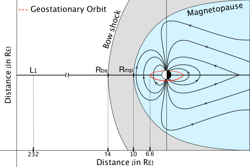
Figure 2: A schematic of the stand-off distance of the MP ($R_{\textrm{mp}}$) and BS ($R_{\textrm{bs}}$) in the GSM coordinate system. The dotted red circle in the equatorial plane represents the geostationary orbit at 6.6 earth radii. The L1 Lagrangian point of the sun-earth system is at 232 earth radii.

Figure 2 shows a schematic representation (not to scale) of the position and the shape of the MP and BS in the GSM coordinate system wherein, the earth is considered to be at the origin. The x-axis is along the sun-earth line, the z-axis is perpendicular to the plane of the earth’s orbit. $R_{\textrm{bs}}$ and $R_{\textrm{mp}}$ represent stand-off distances of the BS and MP, respectively. The nominal positions of the stand-off distances of the MP and BS at 10 and 14 earth radii (R_E) respectively, are indicated. Also shown, by a red circle at 6.6 R_E, is the geostationary orbit in the earth’s equatorial plane and the location of the Lagrangian point, L1, of the sun-earth system at 232 R_E.

In order to compute the stand-off distance of the BS and the MP, we used daily averaged data of solar wind proton density, solar wind velocity, and IMF from Jan. 1975$-$Dec. 2016. The solar wind dynamic pressure was then derived using solar wind proton density ($N_{p}$) and velocity($v_{\textrm{sw}}$). The data sets were obtained from the OMNI data base, a compilation of near-earth magnetic field data and various other plasma parameters from several spacecraft at geocentric or L1 orbit which have been extensively cross compared and normalized (http://gsfc.nasa.gov/omniweb). In the OMNI data base for high resolution data (1-min and 5-min average), interpolations are usually performed on the phase front normal directions (for gap intervals of less than 3 hours), and the time shift (for gap intervals of less than one hour). For the purpose of this study we used low resolution (daily average) data, for which no interpolation was performed. Therefore, after obtaining the OMNI data set, we replaced bad or missing values by the method of index aware interpolation, where the time of observation serves as index.

Various numerical/analytical as well as empirical models have been developed and used to estimate the location and shape of the MP and BS. Numerical models (Nemecek & Safrankova, 1991; Cairns & Lyon, 1995; Peredo et al., 1995; Elsen & Winglee, 1997; Chapman & Cairns, 2003; GarcíA & Hughes, 2007) in general are evaluated using the condition of pressure balance between the solar wind dynamic pressure and the pressure due to the earth’s dipole magnetic field (Chapman & Ferraro, 1931; Zhigulevsk & Romishevskii, 1959; Beard, 1960; Spreiter & Briggs, 1962; Mead & Beard, 1964; Olson, 1969). While most of the empirical models, (Fairfield, 1971; Formisano, 1979; Sibeck et al., 1991; Shue et al., 1997, 1998; Boardsen et al., 2000; Lin et al., 2010; Jelínek et al., 2012) with few exceptions (Wang et al., 2013; Shukhtina & Gordeev, 2015), assume a functional form for the MP and then estemate the corresponding free parameters using available MP crossing database.

Each approach has several limitations, e.g., numerical/analytical models often use an impermeable, infinitely conducting MP as an obstacle, which is far from reality. On the other hand most of the empirical models are restricted to low latitudes. Also, models that use upstream parameters to describe the location and the shape of the MP and BS, implicitly assume proportionality between upstream parameters and their downstream values. This in turn, may lead to significant inaccuracies in cases of extreme solar wind conditions.

While empirical models provide the average values of MP and BS, which are in good agreement with their observational values, it is important to note that since our principle aim is to study the response of the MP and BS to the long term and steady decline in activity seen on the sun and in th solar wind (Janardhan et al., 2010, 2011; Bisoi et al., 2014a; Janardhan et al., 2015), our approach is concentrated on estimating the long term trend and changes in the MP and BS stand-off distance and the MP shape. Therefore, in what follows we estimate the MP stand-off distance using models due to Lin et al. (2010), and Lu et al. (2011), as being representative of empirical and numerical models, respectively. Similarly, the BS stand-off distance has been estimated using Jelínek et al. (2012) and Chapman & Cairns (2003) as being representative of empirical and numerical models, respectively.

3.1 MP stand-off distance

The boundary between the solar wind and magnetosphere can be derived using the pressure balance condition. This condition supposes that the MP and BS can be described as second order surfaces i.e. a surface described by an algebraic equation of degree two. Most of the time therefore, elliptic or parabolic functional forms are used to represent the shape of the MP and BS. However elliptic or parabolic functional forms are generally, not appropriate in describing the MP tail and Shue et al. (1997) proposed the following functional form,

$$r=r_{mp}\left(\frac{2}{1+\cos\theta}\right)^{\alpha}\,\,\,R_{E}.$$ (1)

Equation (1) has two parameters ${\it{viz.}}$ r_mp, the MP stand-off distance and $\alpha$, the flaring parameter. Angle $\theta$ is the solar zenith angle (the angle between the Sun-Earth line and the radial direction) of the point of interest (Shue & Song, 2002). Eq. (1) represents an open MP tail for $\alpha>0.5$ and a closed MP tail for $\alpha<0.5$.

We now briefly describe the models we used in the calculations of the of the MP stand-off distance and MP shape. The first one is due to Lin et al. (2010) which represents an empirical approach, whereas second model, Lu et al. (2011) is representative of a numerical approach.

3.1.1 Empirical model (Using Lin et al., 2010)

Lin et al. (2010), abbreviated as L10 hereafter, extended the assumptions of Shue et al. (1998) to address asymmetries and indentations near the polar cusps. Employing a database of nearly 2708 MP crossings from observations by Cluster, Geotail, Goes, IMP8, Interball, LANL, Polar, TC1, THEMIS, WIND and Hawkeye, along with corresponding solar wind parameters from ACE, Wind and OMNI, they obtained a model for the MP which was parametrised by the solar wind dynamic and magnetic pressure (P_d + P_m), IMF B_z and dipole tilt angle ($\psi$), which is the dipole magnetic latitude of the subsolar point. Based on the relation between P_d and r_mp, the influence of IMF B_z on r₀ (Shue et al., 1998) and the saturation effect of a southward IMF B_z on r_mp (Yang et al., 2003), L10 expressed the stand-off distance for MP as:

$$r_{mp}=a_{0}(P_{d}+P_{m})^{a_{1}}\left(1+a_{2}\frac{\textrm{exp}(a_{3}B_{z})-1}{\textrm{exp}(a_{4}B_{z})-1}\right)\,\,\,R_{E}$$ (2)

The coefficients ($a_{0}$, $a_{1}$, $a_{2}$, $a_{3}$ and $a_{4}$) in equation (2) are obtained by using nonlinear multi parameter fitting (Levenberg $-$ Marquardt method) based on observations of 247 MP crossings that were found near the stand-off distance. The coefficients are listed in Table$-$2 of L10.

To obtain the MP shape, L10 expanded the eq. (1) as,

$$r=r_{mp}\left\{\mathrm{cos}\frac{\theta}{2}+a_{5}\cdot\mathrm{sin}(2\theta)[1+\mathrm{exp}(-\theta)]\right\}^{\beta}\,\,R_{E}.$$ (3)

Where the factor $1-exp(-\theta)$ smooths out the MP shape near the subsolar point. The asymmetries and indentations are introduced through the azimuthal angle $\phi$, the angle between the projection of r in Y-Z plane and the direction of positive Y axis. The flaring parameter $\beta$ (given by equation (5) of L10) is,

$$\beta=\beta_{0}+\beta_{1}\mathrm{cos}(\phi)+\beta_{2}\mathrm{sin}(\phi)+\beta_{3}\mathrm{sin}^{2}(\phi).$$ (4)

We considered the simpler case: $\phi=0$ (meridional plane) for which equation (4) reduces to $\beta=\beta_{0}+\beta_{1}$. $\beta_{0}$ and $\beta_{1}$ (eq. 16 and 17 of L10) are obtained using observations of 422 MP crossings. The relevant values of the parameters are listed in table$-$6 of L10.

The L10 model (eqs 2 and 3) yields good results in predicting MP stand-off distance and MP shape respectively. When compared with the observed low latitude MP crossings, the standard deviation of the L10 model is the least (0.54 $R_{E}$) among several other models.

3.1.2 Numerical model (using Lu et al., 2011)

The second model we used is due to Lu et al. (2011), abbreviated as L11 hereafter, based on global MHD simulations to estimate the MP stand-off distance and the MP shape. L11 analyses the relation between the MP and the IMF B_z and P_d using numerical results from a global MHD model Space Weather Modelling and Framework (SWMF), a framework for physics-based space weather simulations (Tóth et al., 2005). A streamline technique was used to identify the location and shape of the MP. The functional form of Shue et al. (1997) was extended to describe the global MP size and shape using the method of multi-parameter fitting. L11 included azimuthal asymmetry via ($\phi$) and extended the functional form in eq. (1). The dayside MP is given by,

$$r=r_{mp}\left(\frac{2}{1+\mathrm{cos}\theta}\right)^{\alpha+\beta_{1}\mathrm{cos}\phi}\,\,R_{E}.$$ (5)

Where $\beta_{1}$ characterises the azimuthal asymmetry with respect to $\phi$. Using fitting results from Shue et al. (1997), the relationship between the (r₀, $\alpha$, $\beta_{1}$) and solar wind conditions (P_d, B_z) was evaluated. The multiple parameter fitting results in the following best-fit functions (eq., 18, 19, 20 of L11):

$$r_{mp}=\begin{cases}(11.494+0.0371B_{z})P_{d}^{-1/5.2},\,\,B_{z}\geq 0\\ (11.494+0.0983B_{z})P_{d}^{-1/5.2},\,\,B_{z}<0\end{cases}$$ (6)

$$\alpha=\begin{cases}(0.543-0.0225B_{z}+0.00528P_{d}+\\ 0.00261B_{z}P_{d}),\,\,B_{z}\geq 0\\ (0.543-0.0079B_{z}+0.00528P_{d}+\\ 0.00019B_{z}P_{d}),\,\,B_{z}<0\end{cases}$$ (7)

$$\beta_{1}=\begin{cases}(-0.263+0.0045B_{z}-0.00924P_{d}-\\ 0.00059B_{z}P_{d}),\,\,B_{z}\geq 0\\ (-0.263-0.0259B_{z}-0.00924P_{d}+\\ 0.00256B_{z}P_{d}),\,\,B_{z}<0\end{cases}$$ (8)

The model due to L11 yields good matching when compared with the high and low latitude MP crossings.

3.2 BS stand-off distance

The shape and the location of the BS mainly depends on the location of the MP as well as various solar wind parameters, for example the magnetosonic and Alfvén Mach numbers. In general, the shape of the BS is assumed to be a paraboloid along the Earth $-$ Sun line. We now briefly describe the models we used in the calculations of the BS stand-off distance. The first model, Jelínek et al. (2012) represents an empirical approach and the second one, Chapman & Cairns (2003), is a representative of numerical approach.

3.2.1 Empirical model (Jeĺinek et al. 2012)

Jelínek et al. (2012), hereafter abbreviated as J12, investigated the solar wind (SW), magnetosheath (MSH) and magnetosphere (MS) using measurements from the THEMIS spacecraft between March 2007 and September 2009. The orbits of the five THEMIS spacecraft spans all three regions of interest: SW, MSH and MS. The ACE spacecraft at L1 was used as a solar wind monitor. The ratio of the measurements of the magnetic field and density from THEMIS with those from ACE enables one to identify SW, MSH and MS and the boundaries between these regions for the entire day-side part. Since BS and MP are often described as second order surfaces, J12 expected a parabolic shape for both of the boundaries that responds to the upstream dynamic pressure, P_d as,

$$r\sim P_{d}^{-1/\epsilon}.$$ (9)

J12 assumes rotationally symmetric BS and MP around the $X_{GSM}$. An analytic expression for the BS and MP is used and the free parameters are determined using least square fitting to the full data set. However the MP model due to Jelínek et al. (2012) does not include the effect of the dipole tilt angle, which is the dipole magnetic latitude of the subsolar point, and is therefore severely restricted to the low latitudes, whereas the L10 model described in §3.1.1 is applicable in more general situations. We therefore only considered the model of the BS stand-off distance from the Jelínek et al. (2012), given by.

$$r_{bs}=15.02P_{d}^{-1/6.55}\,\,\,R_{E}.$$ (10)

Although the equation (10) does not take into account the Mach number, this simple model was found in good agreement when compared with more than 6000 BS crossings.

3.2.2 Numerical model (Chapman & Cairns 2003)

The model due to Chapman & Cairns (2003), hereafter abbreviated as CC03, uses 3D ideal MHD simulations (Cairns & Lyon, 1995), which in turn uses an impermeable infinitely conducting magnetopause (given by Farris et al. (1991)) as an obstacle. This model is parametrised by P_d, the Alfvén Mach number (M_A) and the orientation of the IMF ($\theta_{IMF}$) with respect to the direction of the solar wind velocity ($v_{sw}$). Chapman & Cairns (2003) considers two special cases of $\theta_{IMF}=45^{\circ}$ and $90^{\circ}$, of which we use $\theta_{IMF}=90^{\circ}$ to estimate the BS stand-off distance given by

$$r_{bs}=\left(\alpha_{0}+\frac{\alpha_{1}}{M_{A}}\right)\left(\frac{P_{d}}{1.87}\right)^{-1/6}\,\,\textrm{$R_{E}$}.$$ (11)

Here, ($\alpha_{0},\alpha_{1}$) are the fitting parameters obtained by least square fitting to the simulated shock locations. The CC03 model has been compared with available spacecraft data close to the nose region of the BS and it was found that for the near-Earth regime ($-20R_{E}<x<35R_{E}$), the model does well in predicting the BS location.

4 Results

One of the key parameters in determining the shape and location of the BS and MP is their stand-off distance, which depends principally on P_d and the strength of the IMF. Therefore, the variations in the stand-off distances as a function of P_d and IMF gives one a good handle in understanding the response of the earth’s magnetosphere to the changes in solar wind conditions and in turn to the global variability in solar activity. We now present and compare the results for the BS stand-off distance obtained by using empirical (Jelínek et al., 2012) and numerical (MHD) model (Chapman & Cairns, 2003), described in (§3.2.1) and (§3.2.2 respectively.)

We have computed the BS stand-off distance and normalised it to its average value subjected to the typical solar wind conditions at 1 AU. This has been done to show the excursions of the BS beyond the average stand-off distance for cycles $21-24$. For typical solar wind conditions at 1 AU (P_d $\sim$1.87 nPa, B = 7 nT, N_p = 6.6 cm^-3; M_a = 8), the average BS stand-off distance according to J12 is $13R_{E}$ and that of due to CC03 is $18R_{E}$. The difference in the magnitude of the BS stand-off distance estimated by these two models can be understood in the following way. Both the models,

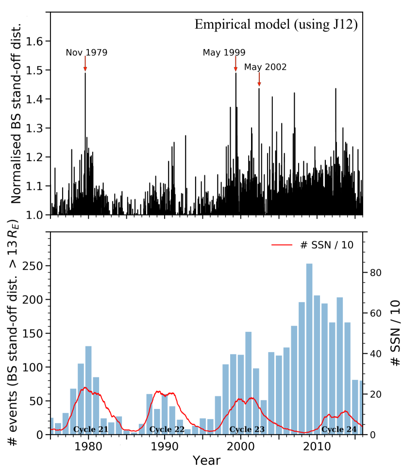
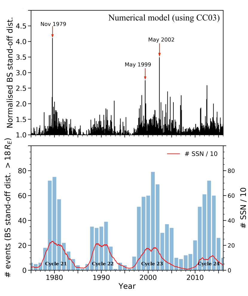
Figure 3: Daily average of the normalized BS stand-off distance between January 1975 and December 2016. Left (top and bottom) panels uses J12, while Right (top and bottom) panels uses CC03. Three extreme events, designated as solar wind disappearance events in the literature, have been labeled with the event dates (upper panels). The distribution of the number of events or instances for which the BS stand-off distance $>$ average stand-off distance between 1975 and 2016 (bottom panels). A 12 month moving average of the sunspot numbers, scaled down by a factor of 10 is shown over plotted (in red) on the histogram.

CC03 and J12 relates BS stand-off distance with solar wind dynamic pressure as a power law, but with different power law indices. Also CC03 model includes the effect of the Alvén Mach number (M_A), which is neglected in J12.

In Figure 3 left panels (top and bottom) shows the results obtained by using an empirical model (J12, §3.2.1) and right panels (top and bottom) shows results obtained by using a numerical model (CC03, §3.2.2). The upper panel (top left and right) of Fig. 3 shows the daily average of the normalized BS stand-off distance from 1975 to December 2016, derived using J12 (top left) and CC03 (top right). It is clear that the normalized BS stand-off distance, on an average, follows the eleven year solar cycle. Surprisingly though, such excursions of the BS well beyond average stand-off distance are not rare and are much more frequent than expected. From the upper panel of Fig.3 it is clear that, irrespective of the model used there are a large number of cases of the BS stand-off distance extending well beyond the average value. Three such events are indicated in the Fig.3 (upper panel). These events have been well studied and are referred to as solar wind disappearance events (Balasubramanian et al., 2003; Janardhan et al., 2005, 2008a, 2008b) due to the extremely low densities observed at 1 AU ($<$ 0.1 $\textrm{cm}^{-3}$) for periods exceeding 24 hours. During all three events, a sharp decrease in $P_{d}(<0.02~{}\textrm{nPa}$) was seen indicating sensitive response of the BS stand-off distance to solar wind conditions.

To quantify the effect of the solar wind conditions on the BS, we selected events for which the BS stand-off distance increases more than 1$\sigma$ of the average value of the BS stand-off distance. The lower panel of Fig. 3 (lower left and right) shows the histogram of the distribution of the number of events for the years between 1975 and 2016 obtained using J12 (lower left) and CC03 (lower right). As stated earlier, it is clear that BS excursions beyond average distance are not rare but are observed consistently in each solar cycle. However, there is a significant increase in the number of events since $\sim$1995 when solar photospheric magnetic fields began declining. The increase was found to be more than 40% when compared with the number of events before 1995. Note that the increase in the number of events is irrespective of the models used.

We now turn to the discussion of the MP stand-off distance and the MP shape obtained by empirical (Lin et al., 2010) and numerical (MHD) models (Lu et al., 2011), described in (§3.1.1) and (§3.1.2) respectively. The MP stand-off distance for the years Jan. 1975$-$Dec. 2016 is shown in Figure 4. The top panel shows the result obtained by using L10 whereas, the results in the lower panel are derived using L11. The grey dots are monthly averages of the MP stand-off distance. The blue circles represent annual averages shown with 1$\sigma$ error bars. The monthly averaged sunspot number, scaled down by a factor of 10, is shown by a grey solid line with the smoothed value (one year moving average) over plotted in blue. It is clear from the figure that the MP stand-off distance is sensitive to and is modulated, with a periodicity of 11 years, by the solar cycle.

To remove this periodicity and investigate the trend, daily average of the MP stand-off distance was smoothed using a eleven year running mean, shown by the over plotted solid red curve in Fig. 4, which shows a clear increasing trend in the MP stand-off distance starting in $\sim$1995, and monotonically increasing till 2015. The increase is $\sim 15\%$, irrespective of the models used.

We also determined the shape of the MP. Following the standard GSM coordinate system we computed position of the MP, $X_{s}=rsin(\theta)$ and $R_{s}=rcos(\theta)=\sqrt{(}Y^{2}+Z^{2})$, where $\theta$ is the solar zenith angle. $R_{s}$ is interpreted as the transverse radius. We refer to the plot of $R_{s}$ v/s $X_{s}$, averaged over 11 years, as the shape of the MP or MP shape.

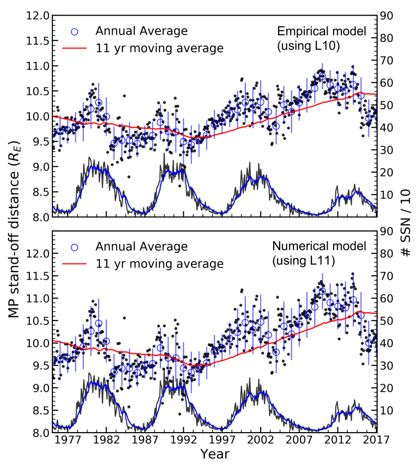
Figure 4: Monthly averages of the MP stand-off distance for the period Jan. 1975$-$Dec. 2016 (grey filled circles) derived using Lin et al. (2010) (L10) (upper panel) and Lu et al. (2011) (L11) (lower panel). The blue circles represent annual averages shown with 1$\sigma$ error bars. The red line is a eleven year moving average of the daily average of the MP stand-off distance. The monthly averaged sunspot number, scaled down by a factor of 10, is shown by the solid curve in grey with the smoothed value (one year moving average) over plotted in blue.

Figure 5 shows the plot of $R_{s}$, the transverse radius against $X_{s}$ the stand-off distance along the earth-sun line for the day-side MP and for a solar zenith angle between $\theta$ = 0^∘ and $\theta$ = 90^∘. Upper panel of the Fig. 5 shows the MP shape obtained using eq. (3) (§3.1.1), whereas lower panel shows the MP shape derived using eq. (5) (§3.1.2).

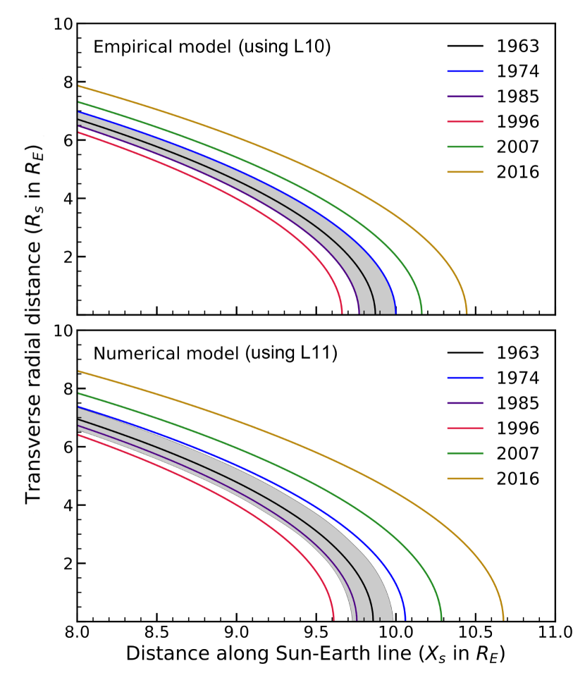
Figure 5: The 11 year averaged MP shape shown by a plot of the transverse radial distance of the MP, $R_{s}$ against the extent of the MP along the sun-earth line, $X_{s}$. The upper panel uses Lin et al. (2010) (L10) (§3.1.1) and the lower panel uses Lu et al. (2011) (L11) (§3.1.2). The black line is the eleven year average starting from 1963, with shaded gray band having a 1$\sigma$ width. The blue, indigo, red, green and gold curves represent 11 year averaged MP shapes for years 1974, 1985, 1996, 2007 and 2016, respectively.

The average MP shape is labeled by the starting year, e.g. the MP shape of 1963, shown by the black curve, refers to the MP shape that is averaged over the eleven years starting from 1963. The gray band in Fig. 5 signifies the region of 1$\sigma$ around the MP shape of 1963. It is important to note that, in case of L10 (upper panel), the MP shape of 1974 and 1985 falls within this gray band. Whereas, in case of L11 (lower panel) the average MP shape for the year 1974 is slightly outside the 1$\sigma$ region of the MP shape of 1963. However, in both cases (L10 and L11) the average MP shape in 1996 falls well below the average MP shape of 1974, and then bounces forward significantly in 2007 and continues to expand till 2016. It can be seen that the expansion of the MP is different at different MP positions but there is an overall expansion in MP with the maximum expansion being at the stand-off point. For the period between 1996 and 2016, the stand-off point expanded by nearly 1 R_E from $\sim$9.6 R_E to $\sim$10.5 R_E, irrespective of the model used.

5 Discussion and conclusions

We have carried out an extensive study based on IMF and solar wind data between January 1975 and December 2016. Owing to the complex nature of the solar wind - magnetosphere interaction, determining the boundaries (BS and MP) is an open question. At the present time accurate theoretical and observational models for the shape and location of the BS and MP do not exist. However, our aim was to investigate the response of the stand-off distance of the BS and MP to the observed decline in solar activity - characterised by the change in the high latitude magnetic field (Janardhan et al., 2015) and micro-turbulence levels over the heliocentric distance between 0.2 to 0.8 AU (Janardhan et al., 2011). We therefore carried out the calculations and compared the results for several available models. We presented the results for the MP stand-off distance and the MP shape using L10 (empirical model, §3.1.1) and compared them with the results obtained from L11 (global MHD simulations, §3.1.2). For the BS stand-off distance we presented the results using CC03 (Global MHD simulations, §3.2.1) and compared them with the results obtained by J12 (empirical model, §3.2.2). We found that the long term trend in the BS and MP as a response to solar wind conditions and IMF is, in general, independent of the model used.

The stand-off distance of the MP and BS are sensitive to variations in P_d and IMF B_z. They are also affected by the Alfvén and magnetosonic Mach numbers. The angle between the magnetic field and the solar wind velocity vector is critical in determining the shock location of the BS (Cairns & Lyon, 1995). The shape of the magnetopause is asymmetric due to the cusp in the polar regions, this asymmetry can be accounted if the dipole tilt angle ($\psi$) is taken into consideration (Lin et al., 2010; Shukhtina & Gordeev, 2015). To simplify the analysis we considered MP and BS symmetric about the sun-earth line (i.e. the X-axis of the GSM coordinate system) and neglected the dipole tilt angle. For calculating BS stand-off distance using CC03 we kept IMF angle ($\theta$) fixed at $90^{\circ}$.

A decrease in P_d and IMF causes an expansion of the BS and MP, resulting in an increase in their sub-solar distances. The stand-off distance of the MP, in general, exhibits a power law dependence on the dynamic pressure, with power law index $\sim-1/6$ (Mead & Beard, 1964; Petrinec & Russell, 1996). A self-similar scaling suggests an identical power law dependence for the stand-off distance of the BS (Cairns & Lyon, 1996). However, the power law index found in several empirical as well as numerical studies is little less than $-1/6$. This reduced value might be the effect of the pressure due to earth’s dipole field (Jelínek et al., 2012). It is worth noting here that both approaches numerical/analytical and empirical either implicitly or directly include the earth’s dipole field. Zhong et al. (2014) have shown that the earth’s dipole moment has been decaying over the past 1.5 centuries. Assuming linear rate of decay to persist their results suggests, the average stand-off distance of the MP would move $\sim 0.3R_{E}$ towards the earth per century. We are looking for trend in the MP stand-off distance averaged over the eleven years and computing eleven year average of the MP shape so the modification to the MP shape at subsolar point due to the change in the pressure caused by declining dipole field will be very small and hence negligible.

The main conclusions of the paper are:

1. Corresponding to the observed decrease of $\sim$40% in P_d, a steady increase of $\sim$15% was observed in the stand-off distance of the MP which can be attributed to the power law dependence.

2. We also observed a significant increase of more than 40% in the number of events (after 1995) where the stand-off distance of the BS exceeded the average stand-off distance over the past $\sim$20 years, when compared with the number of events prior to 1995. This indicates that the earth’s magnetosphere is very sensitive to the changes in solar wind conditions.

3. From our study of the variation in the 11 year average shape of MP, we found that the MP, since 1996, has undergone a significant expansion which is highest at the stand-off point and narrows down towards the transverse radius. Our result for the shape of the MP is consistent with the increase in the stand-off distance of the MP reported by McComas et al. (2013) wherein, they found an increase in the stand-off distance of the MP from 10 $R_{E}$ in 1974$-$1994 to 11 $R_{E}$ in 2007–2013. The values of P_d and the stand-off distance of MP, from 1974$-$1994, were respectively, $\sim$2.9 nPa and 9.7 R_E. In contrast, these values, from 1995$-$2017, were found to be respectively, $\sim$2.0 nPa and 10.7 R_E. So our results of the increase in the MP stand-off distance ($\sim$9.3%) are consistent with the increase in stand-off distance of MP ($\sim$10%) reported by McA13. Our results also showed an increase in MP shape ($>$ 10 $R_{E}$) for the period from 2007$-$2016.

4. During solar minimum, photospheric high latitude magnetic fields extend to low latitudes and are then pulled into the heliosphere by the solar wind thereby, forming the IMF (Schatten & Pesnell, 1993). The changes in the solar wind conditions such as decline in P_d and IMF strength can thus be interpreted as being induced by global changes in the solar magnetic fields. Our study underlines the causal relation between solar activity changes and the corresponding global response of the earth’s magnetosphere via the variations quantified by the stand-off distances of the BS and MP.

5. The present work quantifies the response of the earth’s magnetosphere via the variations in the stand-off distance of the MP and BS subjected to the lomg term changes in P_d and IMF. We have found that both the P_d and the IMF have been steadily declining since $\sim$1995 with the reduction in their average values over the last 20 years being $\sim$40%. This is consistent with the ongoing declining trend in high-latitude photospheric magnetic fields and solar wind micro-turbulence levels, both of which showed a decrease in their strength beginning around $\sim$1995.

6. We find that the steady decline in high-latitude photospheric fields and solar wind micro-turbulence levels are still continuing implying low sunspot activity in future, a condition akin to the Maunder minimum. Using a global thermodynamic model, Riley et al. (2015) reported the likely state of the solar corona, during the later period of the Maunder minimum, devoid of any large scale structure and driven by a reduced photospheric magnetic field strength. The photospheric field strength during the last two solar cycles has been steadily decreasing (since $\sim$1995) and the trends indicate that it is likely to decline in the same manner in future solar cycles. This implies a state of corona with no large scale structure much alike Maunder minimum period, which in turn, leads to a highly bulged terrestrial magnetosphere with an increased stand-off distance for the bow shock and the magnetopause.

Continued investigation to understand and forecast the influence of solar activity on the near earth environment and the ecosystem is therefore of considerable importance.

References

- Ananthakrishnan et al. (1995) Ananthakrishnan, S., Balasubramanian, V., & Janardhan, P. 1995, Space Sci. Rev., 72, 229
- Ananthakrishnan et al. (1980) Ananthakrishnan, S., Coles, W. A., & Kaufman, J. J. 1980, J. Geophys. Res., 85, 6025
- Balasubramanian et al. (2003) Balasubramanian, V., Janardhan, P., Srinivasan, S., & Ananthakrishnan, S. 2003, J. Geophys. Res., 108, 1121
- Beard (1960) Beard, D. B. 1960, J. Geophys. Res., 65, 3559
- Bisoi et al. (2014a) Bisoi, S. K., Janardhan, P., Chakrabarty, D., Ananthakrishnan, S., & Divekar, A. 2014a, Sol. Phys., 289, 41
- Bisoi et al. (2014b) Bisoi, S. K., Janardhan, P., Ingale, M., et al. 2014b, ApJ, 793, 8
- Boardsen et al. (2000) Boardsen, S. A., Eastman, T. E., Sotirelis, T., & Green, J. L. 2000, J. Geophys. Res., 105, 23,193?23,219
- Cairns & Lyon (1995) Cairns, I. H., & Lyon, J. G. 1995, J. Geophys. Res., 100, 17173
- Cairns & Lyon (1996) —. 1996, Geophys. Res. Lett., 23, 2883
- Chapman & Cairns (2003) Chapman, J. F., & Cairns, I. H. 2003, Journal of Geophysical Research (Space Physics), 108, 1174
- Chapman & Ferraro (1931) Chapman, S., & Ferraro, V. C. A. 1931, Terr. Magn. Atmos. Electr., 36, 77
- Clette & Lefèvre (2016) Clette, F., & Lefèvre, L. 2016, Sol. Phys., 291, 2629
- Cliver (2016) Cliver, E. W. 2016, Sol. Phys., 291, 2891
- Cliver & Ling (2011) Cliver, E. W., & Ling, A. G. 2011, Sol. Phys., 274, 285
- Elsen & Winglee (1997) Elsen, R. K., & Winglee, R. M. 1997, J. Geophys. Res., 102, 4799
- Fairfield (1971) Fairfield, D. H. 1971, J. Geophys. Res., 76, 6700
- Fairfield et al. (2001) Fairfield, D. H., Cairns, I. H., Desch, M. D., et al. 2001, J. Geophys. Res., 106, 25361
- Farris et al. (1991) Farris, M. H., Petrinec, S. M., & Russell, C. T. 1991, Geophys. Res. Lett., 18, 1821
- Formisano (1979) Formisano, V. 1979, Nuovo Cimento C Geophysics Space Physics C, 2, 681
- Fujiki et al. (2016) Fujiki, K., Tokumaru, M., Hayashi, K., Satonaka, D., & Hakamada, K. 2016, ApJ, 827, L41
- GarcíA & Hughes (2007) GarcíA, K. S., & Hughes, W. J. 2007, Journal of Geophysical Research (Space Physics), 112, A06229
- Gopalswamy et al. (2016) Gopalswamy, N., Yashiro, S., & Akiyama, S. 2016, ApJ, 823, L15
- Janardhan & Alurkar (1993) Janardhan, P., & Alurkar, S. K. 1993, A&A, 269, 119
- Janardhan et al. (2011) Janardhan, P., Bisoi, S. K., Ananthakrishnan, S., Tokumaru, M., & Fujiki, K. 2011, Geophys. Res. Lett., 38, L20108
- Janardhan et al. (2015) Janardhan, P., Bisoi, S. K., Ananthakrishnan, S., et al. 2015, Journal of Geophysical Research (Space Physics), 120, 5306
- Janardhan et al. (2010) Janardhan, P., Bisoi, S. K., & Gosain, S. 2010, Sol. Phys., 267, 267
- Janardhan et al. (2005) Janardhan, P., Fujiki, K., Kojima, M., Tokumaru, M., & Hakamada, K. 2005, J. Geophys. Res., 110, 8101
- Janardhan et al. (2008a) Janardhan, P., Fujiki, K., Sawant, H. S., et al. 2008a, J. Geophys. Res., 113, 3102
- Janardhan et al. (2008b) Janardhan, P., Tripathi, D., & Mason, H. E. 2008b, å, 488, L1
- Jelínek et al. (2012) Jelínek, K., Němeček, Z., & Šafránková, J. 2012, Journal of Geophysical Research (Space Physics), 117, A05208
- Jian et al. (2011) Jian, L. K., Russell, C. T., & Luhmann, J. G. 2011, Sol. Phys., 274, 321
- Lin et al. (2010) Lin, R. L., Zhang, X. X., Liu, S. Q., Wang, Y. L., & Gong, J. C. 2010, Journal of Geophysical Research (Space Physics), 115, A04207
- Lopez et al. (2011) Lopez, R. E., Merkin, V. G., & Lyon, J. G. 2011, Annales Geophysicae, 29, 1129
- Lu et al. (2011) Lu, J. Y., Liu, Z.-Q., Kabin, K., et al. 2011, Journal of Geophysical Research (Space Physics), 116, A09237
- McComas et al. (2013) McComas, D. J., Angold, N., Elliott, H. A., et al. 2013, ApJ, 779, 2
- McComas et al. (2003) McComas, D. J., Elliott, H. A., Schwadron, N. A., et al. 2003, Geophys. Res. Lett., 30, 1517
- Mead & Beard (1964) Mead, G. D., & Beard, D. B. 1964, J. Geophys. Res., 69, 1169?1179
- Nemecek & Safrankova (1991) Nemecek, Z., & Safrankova, J. 1991, Journal of Atmospheric and Terrestrial Physics, 53, 1049
- Olson (1969) Olson, W. P. 1969, J. Geophys. Res., 74, 5642
- Peredo et al. (1995) Peredo, M., Slavin, J. A., Mazur, E., & Curtis, S. A. 1995, J. Geophys. Res., 100, 7907
- Petrinec & Russell (1996) Petrinec, S. M., & Russell, C. T. 1996, J. Geophys. Res., 101, 137
- Readhead & Hewish (1972) Readhead, A. C. S., & Hewish, A. 1972, Nature, 236, 440
- Richardson et al. (2001) Richardson, J. D., Wang, C., & Paularena, K. I. 2001, Advances in Space Research, 27, 471
- Riley et al. (2015) Riley, P., Lionello, R., Linker, J. A., et al. 2015, ApJ, 802, 105
- Rout et al. (2017) Rout, D., Chakrabarty, D., Janardhan, P., et al. 2017, Geophys. Res. Lett., L
- Sánchez-Sesma (2016) Sánchez-Sesma, J. 2016, Earth System Dynamics, 7, 583
- Schatten & Pesnell (1993) Schatten, K. H., & Pesnell, W. D. 1993, Geophys. Res. Lett., 20, 2275
- Shue et al. (1997) Shue, J.-H., Chao, J. K., Fu, H. C., et al. 1997, J. Geophys. Res., 102, 9497
- Shue & Song (2002) Shue, J.-H., & Song, P. 2002, Planet. Space Sci., 50, 549
- Shue et al. (1998) Shue, J.-H., Song, P., Russell, C. T., et al. 1998, J. Geophys. Res., 103, 17691
- Shukhtina & Gordeev (2015) Shukhtina, M. A., & Gordeev, E. 2015, Annales Geophysicae, 33, 769
- Sibeck et al. (1991) Sibeck, D. G., Lopez, R. E., & Roelof, E. C. 1991, J. Geophys. Res., 96, 5489
- Spreiter & Briggs (1962) Spreiter, J. R., & Briggs, B. R. 1962, J. Geophys. Res., 67, 37
- Spreiter et al. (1966) Spreiter, J. R., Summers, A. L., & Alksne, A. Y. 1966, Planet. Space Sci., 14, 223
- Tóth et al. (2005) Tóth, G., Sokolov, I. V., Gombosi, T. I., et al. 2005, J. Geophys. Res., 110, 12226
- Usoskin et al. (2007) Usoskin, I. G., Solanki, S. K., & Kovaltsov, G. A. 2007, A&A, 471, 301
- Usoskin et al. (2014) Usoskin, I. G., Hulot, G., Gallet, Y., et al. 2014, A&A, 562, L10
- Verigin et al. (1999) Verigin, M. I., Kotova, G. A., Remizov, A. P., et al. 1999, Cosmic Research, 37, 34
- Wang et al. (2013) Wang, Y., Sibeck, D. G., Merka, J., et al. 2013, Journal of Geophysical Research (Space Physics), 118, 2173
- Yang et al. (2003) Yang, Y.-H., Chao, J. K., Dmitriev, A. V., Lin, C.-H., & Ober, D. M. 2003, Journal of Geophysical Research (Space Physics), 108, 1104
- Zachilas & Gkana (2015) Zachilas, L., & Gkana, A. 2015, Sol. Phys., 290, 1457
- Zhigulevsk & Romishevskii (1959) Zhigulevsk, V. N., & Romishevskii, E. A. 1959, Soviet Phys. Doklady, 5, 1001
- Zhong et al. (2014) Zhong, J., Wan, W. X., Wei, Y., et al. 2014, Journal of Geophysical Research (Space Physics), 119, 9816
- Zolotova & Ponyavin (2014) Zolotova, N. V., & Ponyavin, D. I. 2014, Journal of Geophysical Research (Space Physics), 119, 3281