Abstract

We present an effective method to model empirical action potentials of specific patients in the human atria based on the minimal model of Bueno-Orovio, Cherry and Fenton adapted to atrial electrophysiology. In this model, three ionic are currents introduced, where each of it is governed by a characteristic time scale. By applying a nonlinear optimization procedure, a best combination of the respective time scales is determined, which allows one to reproduce specific action potentials with a given amplitude, width and shape. Possible applications for supporting clinical diagnosis are pointed out.

1 Introduction

Detailed reaction-diffusion models to describe human atrial electrophysiology were first developed in the late 1990s [1, 2, 3, 4] and are further developed until now. Important steps forward have been made to include specific ionic currents [5, 6, 7, 8, 9, 10], which in particular allow one to investigate specific effects of pharmaceuticals in treatments of atrial fibrillation and other heart failures. Complementary to these detailed models, Bueno-Orovio, Cherry and Fenton introduced in 2008 a minimal reaction-diffusion model (BOCF model) for action potentials (AP) in ventricular electrophysiology, where the large number of ionic currents through cell membranes is reduced to three net currents [11]. This model has four state variables, one describing the transmembrane voltage (TMV), and the other three describing the gating of ionic currents. The TMV, as in detailed reaction models, satisfies a partial differential equation of diffusion type with the currents acting as source terms, and the time evolution of the gating variables is described by three ordinary differential equations coupled to the TMV. By fitting the action potential duration (APD), the effective refractory period and the conduction velocity to the detailed model of Courtemanche, Ramirez and Nattel [1] (CRN model), the BOCF model was recently adapted to atrial electrophysiology (BOCF model) [12].

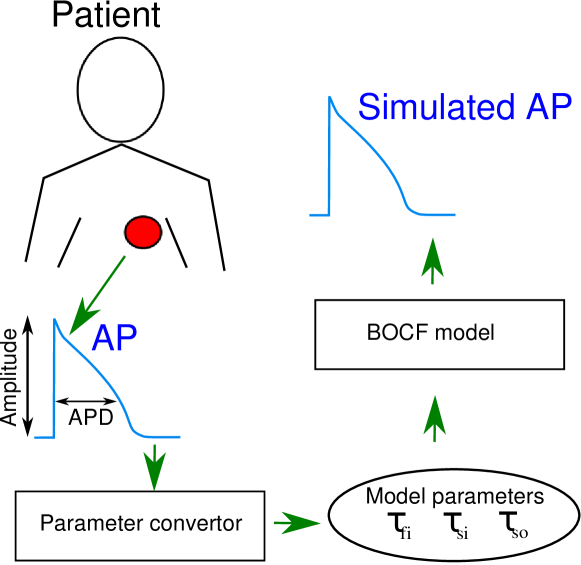
Figure 1: Schematic illustration of the optimized adjustment of the BOCF model by a parameter converter that determines the set of parameter values ($\tau_{\rm fi}$, $\tau_{\rm si}$, and $\tau_{\rm so1}$) giving a best match with the amplitude and duration of the action potential for a specific patient.

In this work we develop a method to model specific AP based on the BOCF model as it is aimed in the clinical context in connection with improved and extended possibilities of diagnosis [13]. Compared to the detailed models, the BOCF model has the advantage that it is better amenable to some analytical treatment. This allows us to identify a small set of relevant model parameters for capturing the main features of a specific AP. Our methodology is sketched in Fig. 1 and can be summarized as follows. We start by labeling each given AP with its amplitude APA and with four APD, namely at 90%, 50%, 40% and 20% repolarization, denoted as APD₉₀, APD₅₀, APD₄₀, and APD₂₀ respectively. These APD_n ($n=20$, 40, 50, 90) together with the amplitude APA are suitable to catch a typical shape of a specific AP, see Fig. 2.

The APD_n taken for a specific patient are given to a parameter convertor that retrieves specific parameter values of the BOCF model. As relevant parameters, we adjust three time scales governing the closing and opening of the ionic channels. The parameter convertor consists of an optimization algorithm that searches for the best set of parameter values consistent with the measured AP properties.

Figure 2: Illustration of an action potential with amplitude APA and four AP durations at 90$\%$, 50$\%$, 40$\%$ and 20$\%$ of the total amplitude. These five values are used to determine three characteristic time scales of the BOCF model (see text).

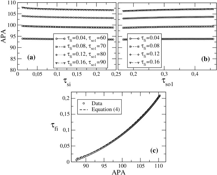
Figure 3: (a) Amplitude APA as a function of $\tau_{\textrm{si}}$ for four different pairs of fixed values $\tau_{\textrm{fi}}$ and $\tau_{\textrm{so1}}$. (b) Dependence of the amplitude APA on time $\tau_{\textrm{so1}}$ for $\tau_{\textrm{si}}=10.7$ ms and four different values of $\tau_{\textrm{fi}}$. (c) Time $\tau_{\textrm{fi}}$ as a function of APA for $\tau_{\rm si}=10.7$ ms and $\tau_{\rm so1}=73.7$ ms.

The paper is organized as follows. In Section 2 we shortly summarize the BOCF model and discuss the role of the three fit parameters that we selected to model specific AP. In Section 3 we show how these parameters can be adjusted to obtain a a faithful representation of the AP properties APA, APD_n, and in Section 4 we demonstrate the specific AP modeling for surrogate data generated with the CRN model [1]. A summary of our main findings and discussion of their relevance is given in Section 5 In the Appendix, we provide analytical calculations for the BOCF model that motivated our choice of fit parameters for the AP modeling.

2 BOCF model for atrial physiology

The BOCF model has four state variables, which are the scaled TMV $u$, and three variables $v$, $w$ and $s$ describing the gating of (effective) net currents through the cell membrane. The TMV $V$ is obtained from $u$ via the linear relation $V=V_{R}(1+\alpha u)$, where for atrial tissue we set $V_{R}=-84.1$ mV for the resting potential and $\alpha=1.02$ [12]. The time-evolution of $u$ is given by the reaction-diffusion equation

$$\partial_{t}u=D\Delta u+J(u,v,w,s)+J_{\textrm{stim}}\,,$$ (1)

where $J=J(u,v,w,s)$ is the total ionic current and $J_{\textrm{stim}}$ an external stimulus current. For modeling of single-cell action potentials, as considered in this work, we set $D=0$. The total ionic current decomposes into three net currents, a fast inward sodium current $J_{\rm fi}=J_{\rm fi}(u,v)$, a slow inward calcium current $J_{\rm si}(u,w,s)$, and a slow outward potassium current $J_{\rm so}=J_{\rm so}(u)$,

$$J(u,v,w,s)=J_{\rm fi}(u,v)+J_{\rm si}(u,w,s)+J_{\rm so}(u)\,.$$ (2)

These currents are controlled by the gating variables, which evolve according to

$$\partial_{t}(v,w,s)=(E(u,v),F(u,w),G(u,s))\,,$$ (3)

where the nonlinear functions $F$, $G$ and $H$, are specified in Section A. There we show that the four differential equations (1) and (3) can be reduced to a system of two differential equations. This reduction shows that the three characteristic times $\tau_{\rm fi}$, $\tau_{\rm si}$ and $\tau_{\rm so1}$, which fix the typical duration of the respective currents, govern the shape of the AP [cf. Eq. (15a) in the Appendix]. We take these three time scales as parameters for fitting a specific AP and keep all other parameters fixed. For the values of the fixed parameters we here consider the set determined for the electrically remodeled tissue due to atrial fibrillation [14, 12].

3 Parameter dependence of BOCF action potentials

In this section we show that in the BOCF model the amplitude APA can be expressed by a quadratic polynomial of the times $\tau_{\rm fi}$, and the APD_n by cubic polynomials of $\tau_{\rm si}$ and $\tau_{\rm so1}$.

The dependence of APA and the APD_n on the characteristic times, was determined from generated AP in single-cell simulations of the BOCF model by applying periodically, with a frequency $f=3$ Hz, a constant stimulus current of $40$ pA, corresponding to an amplitude of $4.76$ s^-1 for the current $J_{\rm stim}$ in Eq. (1), for a time period of $3.5$ ms. The resulting time evolution of the TMV in response to this stimulus was calculated by integrating Eqs. (1) and (3) for the initial conditions $u_{0}=0$, $v_{0}=1$, $w_{0}=1$ and $s_{0}=0$. This was done for $(\tau_{\textrm{fi}},\tau_{\textrm{si}},\tau_{\textrm{so1}})\in[0.002,0.210]\times[5.9,22.4]\times[40,110]$ (in ms) with a resolution $\Delta\tau_{\rm fi}=0.0021$ ms ($100$ values), $\Delta\tau_{\rm si}=0.3$ ms ($56$ values) and $\Delta\tau_{\rm so1}=1$ ms ($71$ values). The AP was recorded after a transient time of 10 s.

As shown for a few representative pairs of fixed values of $\tau_{\rm fi}$ and $\tau_{\rm so1}$ in Fig. 3(a) and 3(b), the APA depends only very weakly on $\tau_{\rm si}$ and $\tau_{\rm so1}$. Neglecting these weak dependencies, on $\tau_{\rm si}$ and $\tau_{\rm so1}$, we find the APA to increase monotonically with $\tau_{\rm fi}$ in the range $[85,110]$ mV relevant for human atria. In Fig. 3(c) we show that the parameter $\tau_{\rm fi}$ can be well described by the quadratic polynomial

$$\tau_{\rm fi}=c_{0}\hbox{APA}^{2}+c_{1}\hbox{APA}+c_{2}\,,$$ (4)

where the coefficients $c_{i}$ and the coefficient of determination $R^{2}$ of the fit are given in Table 1.

Likewise, as demonstrated in Fig. 4(a) for one fixed pair of values of $\tau_{\rm si}$ and $\tau_{\rm so1}$, the APD_n are almost independent of $\tau_{\textrm{fi}}$. Their dependence on $\tau_{\rm si}$ and $\tau_{\rm so1}$, shown in Figs. 4(b)-(e), can be well fitted by the polynomials

$$\hbox{APD}_{n}(\tau_{\rm si},\tau_{\rm so1})=\sum_{m=0}^{3}\sum_{k=0}^{3-m}c^{(n)}_{mk}\tau_{\rm si}^{m}\tau_{\rm so1}^{k}\,.$$ (5)

where the coefficients $c^{(n)}_{mk}$ are listed in Table 1 together with the $R^{2}$ values of the fits.

Table 1: Polynomial coefficients and $R^{2}$ values of the fits of APA to Eq. (4) and of the surfaces APD${}_{n}(\tau_{\rm si},\tau_{\rm so1})$ to Eq. (5). The values of coefficients $c_{mk}^{(n)}$ are given in units of $\hbox{mV}/\hbox{(ms)}^{m+k}$.

Coeffs.	$\mathbf{APA}$	Coeffs.	$\mathbf{APD_{90}}$	$\mathbf{APD_{50}}$	$\mathbf{APD_{40}}$	$\mathbf{APD_{20}}$
Eq. (4)		Eq. (5)
$c_{0}$	2.35	$c^{(n)}_{00}$	$98$	$85$	$84$	$82$
$\pm\Delta c_{0}$	$\pm 0.06$	$\pm\Delta c^{(n)}_{00}$	$\pm 10$	$\pm 10$	$\pm 10$	$\pm 10$
$c_{1}$	-3.8	$c^{(n)}_{10}$	$5.4$	$5.0$	$4.7$	$3.8$
$\pm\Delta c_{1}$	$\pm 0.1$	$\pm\Delta c^{(n)}_{10}$	$\pm 0.3$	$\pm 0.3$	$\pm 0.4$	$\pm 0.3$
$c_{2}$	1.52	$c^{(n)}_{01}$	$-33$	$-33$	$-33$	$-32$
$\pm\Delta c_{2}$	$\pm 0.05$	$\pm\Delta c^{(n)}_{01}$	$\pm 1$	$\pm 1$	$\pm 1$	$\pm 1$
$\mathbf{R^{2}}$	$\mathbf{0.9996}$	$c^{(n)}_{20}$	$0.0001$	$-0.0010$	$0.0001$	$0.003$
		$\pm\Delta c^{(n)}_{20}$	$\pm 0.004$	$\pm 0.004$	$\pm 0.004$	$\pm 0.004$
		$c^{(n)}_{11}$	$-0.40$	$-0.41$	$-0.41$	$-0.43$
		$\pm\Delta c^{(n)}_{11}$	$\pm 0.01$	$\pm 0.01$	$\pm 0.01$	$\pm 0.01$
		$c^{(n)}_{02}$	$2.47$	$2.56$	$2.61$	$2.85$
		$\pm\Delta c^{(n)}_{02}$	$\pm 0.06$	$\pm 0.06$	$\pm 0.07$	$\pm 0.06$
		$c^{(n)}_{30}$	$-0.0000721$	$-0.00005$	$-0.00004$	$-0.00002$
		$\pm\Delta c^{(n)}_{30}$	$\pm 0.00002$	$\pm 0.00002$	$\pm 0.00002$	$\pm 0.00002$
		$c^{(n)}_{21}$	$0.0012591$	$0.00096$	$0.00079$	$0.00018$
		$\pm\Delta c^{(n)}_{21}$	$\pm 0.00007$	$\pm 0.00007$	$\pm 0.00007$	$\pm 0.00007$
		$c^{(n)}_{12}$	$0.0027$	$0.0045$	$0.0057$	$0.0103$
		$\pm\Delta c^{(n)}_{12}$	$\pm 0.0003$	$\pm 0.0003$	$\pm 0.0003$	$\pm 0.0003$
		$c^{(n)}_{03}$	$-0.045$	$-0.050$	$-0.053$	$-0.069$
		$\pm\Delta c^{(n)}_{03}$	$\pm 0.001$	$\pm 0.001$	$\pm 0.001$	$\pm 0.001$
		$\mathbf{R^{2}}$	$\mathbf{0.9956}$	$\mathbf{0.9938}$	$\mathbf{0.9926}$	$\mathbf{0.9866}$

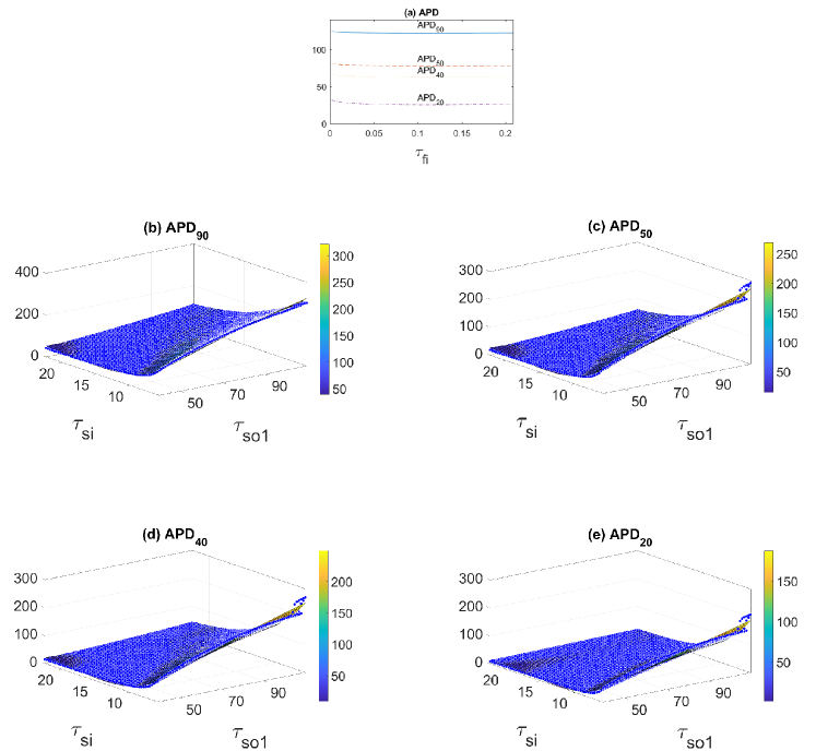
Figure 4: (a) APD_n as a function of $\tau_{\textrm{fi}}$ for a pair of fixed values $\tau_{\textrm{si}}=10.7$ ms and $\tau_{\textrm{so1}}=73.675$ ms. (b)-(e) Dependence of the APD_n on $\tau_{\rm si}$ and $\tau_{\rm so1}$ for fixed $\tau_{\textrm{fi}}=0.0835$ ms. The meshes of points (black bullets) indicate the simulation results, and the surfaces refer to the fits of the meshes, according to Eq. (5). All quantities are given in ms.

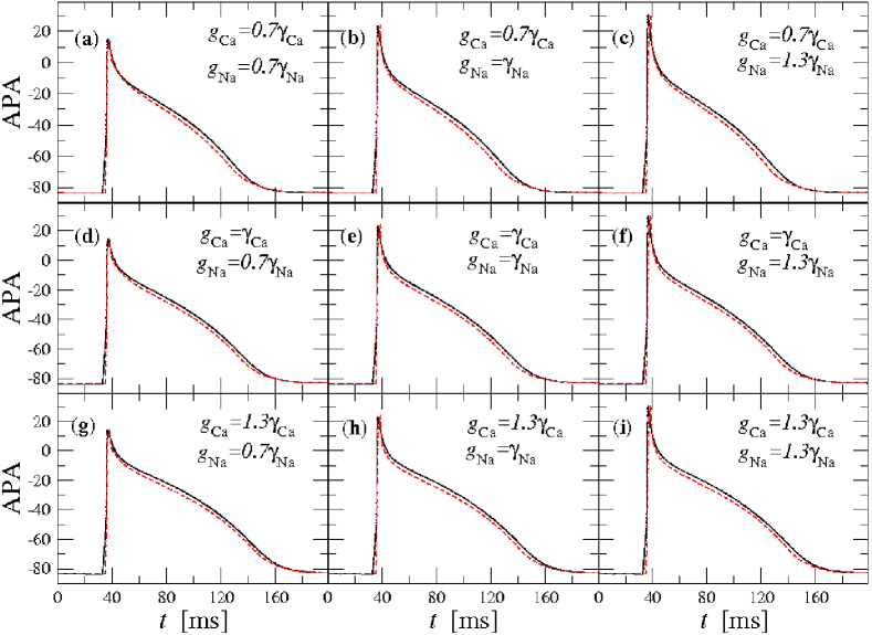
Figure 5: Nine surrogate AP generated with the CRN model (solid lines) for different $g_{\rm Na}$ and $g_{\rm Ca}$ in comparison with the corresponding AP modeled with the BOCF model (dashed lines). The reference values are the ones corresponding to the remodeling case, namely $\gamma_{\rm Ca}=0.0433$ nS$/$ps and $\gamma_{\rm Na}=7.8$ nS$/$ps.

4 Modeling of patient-specific action potentials with the BOCF model

Let us denote by $\mathcal{V}$ the APA and by $\mathcal{D}_{n}$ the values of the APD_n of a specific patient. To model the corresponding AP with the BOCF model, we determine $\tau_{\rm fi}$ by inserting $\hbox{APA}=\mathcal{V}$ in Eq. (4) and $(\tau_{\textrm{si}},\tau_{\textrm{so1}})$ by minimizing the sum of the squared deviations between the the APD_n, i. e. the function

$$\mathcal{F}(\tau_{\rm si},\tau_{\rm so1})=\sum_{n}\big{[}\hbox{APD}_{n}(\tau_{\rm si},\tau_{\rm so1})-\mathcal{D}_{n}\big{]}^{2}\,.$$ (6)

For the numerical procedure we used the Levenberg-Marquardt algorithm [15]. As one sees from Figs. 4(b)-(e), the APD vary monotonically with the time scales in the ranges fixed above. We checked that the Hessian is positive definite in the corresponding region, implying unique solutions when minimizing $\mathcal{F}$.

To demonstrate the adaptation procedure, we generated surrogate AP with the CRN model[1] for electrically remodeled tissue due to atrial fibrillation [14]. Specifically, we consider the maximal conductances, $g_{\rm Ca}$ and $g_{\rm Na}$ of the calcium and sodium currents to vary, while keeping all other parameters fixed to the values corresponding to the electrically remodeled tissue. The conductance $g_{\rm Ca}$ affects both the AP plateau and the repolarization phase and the $g_{\rm Na}$ controls mainly the amplitude of the AP [1].

Figure 5 shows nine examples of AP generated with the CRN model, which cover a wide range of APA and APD. In Figs. 5(a)-(e) we allow $g_{\rm Na}$ and $g_{\rm Ca}$ to differ by factors between $70\%$ and $130\%$ from their values $\gamma_{\rm Na}=7.8$ nS/pF and $\gamma_{\rm Ca}=0.0433$ nS/pF for the electrically remodelled tissue[14]. The corresponding AP modeled with the BOCF, i. e. for $\tau_{\rm fi}$ from Eq. (4), and $\tau_{\rm si}$ and $\tau_{\rm so1}$ obtained from the minimization of $\mathcal{F}(\tau_{\rm si},\tau_{\rm so1})$ in Eq. (6), are shown as dashed lines in the figures. In all cases these reproduce well the AP shapes generated with the CRN model.

Table 2: APA $\mathcal{V}$ and APD_n values $\mathcal{D}_{n}$ for the examples shown in Fig. 5. The $\Delta$ values give the deviations of the individual form parameters according to Eq. (9) and $\Delta\mathcal{A}$ is the deviation between both AP based in their $L_{2}$-norms, as defined in Eq. (7).

		$\mathcal{D}_{90}$	$\mathcal{D}_{50}$	$\mathcal{D}_{40}$	$\mathcal{D}_{20}$	$\mathcal{V}$	$\Delta\mathcal{A}$
		(ms)	(ms)	(ms)	(ms)	(mV)	($\times 10^{-2}$)
Fig.5a	CRN	107.7	66.36	53.07	21.77	98.43
	BOCF	102.9	61.44	48.09	19.26	98.15	4.5
	$\Delta$ ($\times 10^{-2}$)	4.5	7.4	9.4	11.5	0.3
Fig.5b	CRN	106.8	66.02	53.19	23.21	107.14
	BOCF	101.1	60.75	47.73	19.10	107.0	6.0
	$\Delta$ ($\times 10^{-2}$)	5.3	8.0	10.3	17.7	0.15
Fig.5c	CRN	105.9	65.59	53.08	24.04	114.1
	BOCF	100.25	60.71	48.02	19.99	112.9	7.3
	$\Delta$ ($\times 10^{-2}$)	5.3	7.4	9.5	16.8	1.0
Fig.5d	CRN	115.7	72.57	59.03	26.03	98.44
	BOCF	110.5	68.02	53.85	21.59	98.18	4.6
	$\Delta$ ($\times 10^{-2}$)	4.5	6.3	8.8	17.1	0.26
Fig.5e	CRN	114.3	71.75	58.67	27.18	107.1
	BOCF	108.3	66.94	53.17	21.40	107.0	5.9
	$\Delta$ ($\times 10^{-2}$)	5.3	6.7	9.4	21.3	0.08
Fig.5f	CRN	113.2	71.08	58.30	27.84	113.9
	BOCF	107.3	66.64	53.21	22.24	112.9	7.1
	$\Delta$ ($\times 10^{-2}$)	5.3	6.2	8.7	20.1	0.9
Fig.5g	CRN	124.5	81.00	67.44	31.92	98.24
	BOCF	119.6	76.76	62.02	25.66	98.00	4.9
	$\Delta$ ($\times 10^{-2}$)	3.9	5.2	8.0	19.6	0.2
Fig.5h	CRN	122.6	79.69	66.56	32.82	106.9
	BOCF	117.0	75.25	60.92	25.42	106.9	6.2
	$\Delta$ ($\times 10^{-2}$)	4.6	5.6	8.5	22.5	0.02
Fig.5i	CRN	121.2	78.68	65.86	33.30	113.7
	BOCF	115.6	74.59	60.63	26.63	112.8	7.5
	$\Delta$ ($\times 10^{-2}$)	4.7	5.2	7.9	21.2	0.8

To quantify the difference between the AP, we denote by $\mathcal{A}_{\rm CRN}(t)$ and $\mathcal{A}_{\rm BOCF}(t)$ their time course, and compute their relative deviation based on the $L_{2}$-norm,

$$\Delta\mathcal{A}=\frac{||\mathcal{A}_{\rm BOCF}(t)-\mathcal{A}_{\rm CRN}(t)||_{L_{2}}}{||\mathcal{A}_{\rm CRN}(t)||_{L_{2}}}\,,$$ (7)

where

$$||\mathcal{A}(t)||_{L_{2}}\equiv\left(\int_{t_{i}}^{t_{f}}\mathcal{A}^{2}(t)dt\right)^{1/2}\,.$$ (8)

The initial time $t_{i}$ and final time $t_{f}$ are defined as the times for which $u(t_{i})=u(t_{f})=\theta_{0}$ with $\theta_{0}=0.015473$ (see Appendix), with opposite signs of the corresponding time derivatives, i.e. $\tfrac{du}{dt}|_{t_{i}}>0$ and $\tfrac{du}{dt}|_{t_{f}}<0$.

For the examples in Fig. 5, Table 2 gives the values of APA and the APD_n for surrogate AP generated with CRN model and the adapted BOCF model, together with the deviations $\Delta\mathcal{A}$. The largest differences between both AP correspond to deviations of the order of $5\%$ to $7\%$.

The relative errors of the APA and APD_n

$$\Delta=\frac{|X_{\rm BOCF}-X_{\rm CRN}|}{X_{\rm CRN}}\,,$$ (9)

with $X$ representing either $\mathcal{V}$ or $\mathcal{D}_{n}$ are also given in Table 2. The APA show deviations up to $1\%$ and the APD_n up to around $10\%$ for all $n$ except $20$. The APD₂₀ refers to the TMV level closest to the maximum and exhibits larger deviations of about $20\%$ for even small shape deviations.

5 Conclusions

In this work we showed how to model patient-specific action potentials by adjusting three characteristic time scales, which are associated with the net sodium, calcium and potassium ionic currents. The framework explores the possibilities of parameter adjustment of an atrial physiology model, namely the BOCF model[11], to reproduce AP shapes with a given amplitude, width and duration. The BOCF model is defined through a reaction-diffusion equation, coupled to three equations for gating variables that describe the opening and closing of ionic channels. It is simple enough to guarantee low computational costs for even extensive simulations of spatio-temporal dynamics [18]. Through a semi-analytical approach given in the Appendix we showed why the three ionic currents suffice to derive the main features of empirical AP.

The high flexibility for case-specific applications can be used for clinical purposes. Using the optimization procedure for AP shape adjustment, the three characteristic times are retrieved, which are directly connected to the ion-type specific net currents. AP shapes showing pathological features will be reflected in the values of one (or more) times outside acceptable ranges. Accordingly, one can associate a corresponding net current and therefore identify the class of membrane currents, where pathologies should be present. In this sense the clinical diagnosis can be supported by the modeling.

Furthermore, in case information is obtained about AP shapes from different places of the atria, e. g. by using a lasso catheter, a corresponding AP shape modeling would allow one to construct a patient-specific model with spatial heterogeneities. Based on this, it could become possible to generate spatio-temporal activation pattern and to identify possible pathologies associated in the dynamics of the action potential propagation.

Appendix A Appendix: Dynamical features of the BOCF model: a semi-analytical approach.

Figure 6: Time evolution of one AP together with each ionic current: (a) AP variable $u$ with the stimulus current $J_{\rm stim}$, with (b) a close-up for a time interval of $3.5$ ms. Vertical dashed lines intersect the AP at one specific dotted line, thus bounding the time intervals corresponding to each region of $u$-values (see text). The ionic currents correspond to (c) the Na channel ($J_{\rm fi}$), (d) the Ca channel ($J_{\rm si}$), and (e) the K channel ($J_{\rm so}$), see Eqs. (3) and (10). All currents are given in (ms)^-1.

Figure 7: Ionic current (a) $J_{\rm fi}$ and (b) $J_{\rm si}(u,w)$ as a function of the respective gating variables. The red circles indicate the path corresponding to Eqs. (1) and (3) and sketched in Fig. 6 as a function of time. (c) Dependence of ionic current $J_{\rm so}$ on variable $u$.

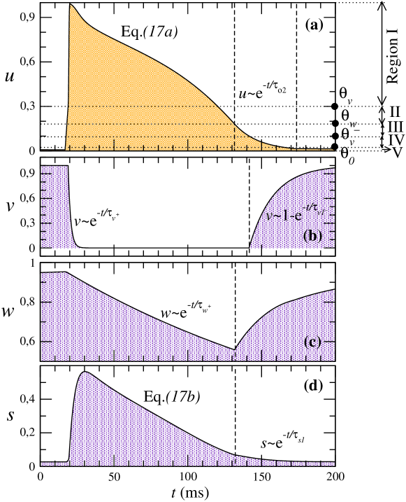
Figure 8: Time evolution of the four variables of the BOCF model: (a) AP variable $u$ and the three gating variables (b) $v$, (c) $w$ and (d) $s$. The horizontal dotted lines in (a) indicate the ranges of $u$-values, where the evolution of the set of variables changes discontinuously. Vertical dashed lines intersect the AP at one specific dotted line, thus bounding the time intervals corresponding to each region of $u$-values. In several of such time intervals, some of the variables decay exponentially and independently from the other variables, which simplifies the model considerably. In the regions where no exponential evolution is indicated the model follows the reduced system of equations in (15): in plot (a) one sees the integration of Eq. (15a) and in plot (d) the integration of Eq. (15b).

Here, we discuss in detail the reaction-diffusion model in Eqs. (1) and (3). We start by considering the terms of the total ionic current $J$, already discussed in Eq. (2. These ionic currents are given by

$$J_{\rm fi} = \frac{v}{\tau_{\rm fi}}(u-\theta_{v})(u_{u}-u)H_{\theta_{v}}(u),$$ (10a)

$$J_{\rm si} = \frac{ws}{\tau_{\rm si}}H_{\theta_{w}}(u),$$ (10b)

$$J_{\rm so} = -\frac{u}{T_{o}(u)}H^{\theta_{w}}(u)-\frac{1}{\tau_{\rm so1}+(\tau_{\rm so2}-\tau_{\rm so1})Q_{\rm so}(u)}H_{\theta_{w}}(u)\,,$$ (10c)

together with the stimulus current

$$J_{\rm stim} = j_{\rm stim}(H_{0}(t^{\ast})-H_{0}(t^{\ast}+T))\,,$$ (11)

where $t^{\ast}=t\hbox{ mod}(1/f)$, $f$ being the frequency of the stimulus signal, $0<T<1/f$ is the duration of the stimulus and $j_{\rm stim}$ being its amplitude. Figure 6 illustrates each of the ionic current together with the stimulus current and the normalized transmembrane voltage. In our simulations we fix $j_{\rm stim}=-40$ pA and $T=3.5$ ms, but similar results are obtained for other stimulus conditions. Function $H_{x}(z)$ is the Heaviside function, equal to $1$ for non-negative $z$ and zero otherwise, and $H^{x}(z)=1-H_{x}(z)$.

Equations (10) (a)-(c) contain further the functions

$$T_{x}(u) = \tau_{x1}H^{\theta_{x}}(u)+\tau_{x2}H_{\theta_{x}}(u)\,,$$ (12a)

$$Q_{x}(u) = \frac{1}{2}\left(1+\tanh{(k_{x}(u-u_{x}))}\right)\,,$$ (12b)

where $u_{u}=1.0089$ and $u_{\rm so}=0.592093$ are reference values, $\theta_{v}=0.3$ and $\theta_{w}=0.18171$ are threshold values of $u$ corresponding to the opening and closing of the ion channels, $\tau_{\rm o1}=250.03$, $\tau_{\rm o2}=16.632$, $\tau_{\rm so2}=6.5537$, and $k_{\rm so}=2.9748$.

As discussed in the main text, current $J_{\rm fi}$ is a fast inward current mediated by sodium channels and controlled by the time scale $\tau_{\rm fi}$, current $J_{\rm si}$ is a slow inward current mediated by calcium channels and controlled by $\tau_{\rm si}$ and current $J_{\rm so}$ is the slow outward current mediated by potassium channels controlled by the time scale $\tau_{\rm so1}$. Figures 6 illustrates each ionic current as a function of time, whereas in Fig. 7 we plot each current as a function of the scaled potential $u$ and the three gating variables.

Both Figs. 6 and 7 may help understanding why the set of the three time scales is suitable for characterizing the full shape of one AP. From Eq. (10a) one sees that for voltages $u>\theta_{v}$ the fast inward current $J_{\rm fi}$ depends linearly on $v$ and quadraticaly on $u$. This current in time shows a very narrow spike (Fig. 6c) which results from a projection over $u$ (Fig. 7a). Thus, the quadratic dependence in $u$ is not as dominant as the linear dependence on $v$ whose slope $1/\tau_{\rm fi}$ parameterizes the height of the spike and consequently the amplitude of the AP. This also explains why the amplitude $V_{A}$ depends more strongly on $\tau_{\rm fi}$ than on the other time scales.

The slow inward current $J_{\rm si}$, Eq. (10b), is only relevant in the range $u>\theta_{w}$ (Fig. 6d) and, for that range, it depends linearly on both $w$ and $s$ gating variables (Fig. 7b) with a slope given by $1/\tau_{\rm si}$.

As for the slow outward current $J_{\rm so}$, Eq. (10b), it depends on $u$ exclusively. It has two mutually exclusive regimes, one for $u<\theta_{w}$ and another for $u>\theta_{w}$. As illustrated in Fig. 7c, for $u<\theta_{w}$ the slow outward current evolves linearly to the transmembrane current, with a slope given by a time scale, $\tau_{o1}$ or $\tau_{o2}$ depending if $u>\theta_{o}$ or $u<\theta_{o}$ respectively. For $u>\theta_{w}$, the current $J_{\rm so}$ varies monotonically with $u$, since it is a bounded step function of $u$ in the range $[0,1]$, and consequently in this range of voltages $J_{\rm so}$ is governed by one of the time scales, $\tau_{\rm so1}$ or $\tau_{\rm so2}$, which we choose to be $\tau_{\rm so1}$.

These three time scales together with the three ionic currents play also a role for defining the full model. As we will see next the set of four equations can be reduced to only two nonlinear equations, which include the dominant parts of each ionic current, and consequently are tunnable through their three time scales.

To see this we start by writing explicitly the three additional functions defining the evolution of the gating variables in Eqs. (1) and (3):

$$E(u,v) = -\frac{v-H^{\theta_{v}^{-}}(u)}{T^{-}_{v}(u)}H^{\theta_{v}}(u)-\frac{v}{\tau^{+}_{v}}H_{\theta_{v}}(u)\,,$$ (13a)

$$F(u,w) = -\frac{w-w_{\infty}}{\tau^{-}_{w1}+(\tau^{-}_{w2}-\tau^{-}_{w1})Q^{-}_{w}(u)}H^{\theta_{w}}(u)-\frac{w}{\tau^{+}_{w}}H_{\theta_{w}}(u)\,,$$ (13b)

$$G(u,s) = \frac{1}{T_{\theta_{w}}(u)}\left(Q_{s}(u)-s\right),$$ (13c)

with

$$w_{\infty}=\left(1-\frac{u}{\tau_{w\infty}}\right)H^{\theta_{o}}(u)+w^{*}_{\infty}H_{\theta_{o}}(u)\,,$$ (14)

$T_{x}(u)$ and $Q_{x}(u)$ are given by Eqs. (12), and $\tau_{v1}^{-}=16.3$, $\tau_{v2}^{-}=1150$, $\tau_{v}^{+}=1.7026$, $\tau_{w1}^{-}=79.963$, $\tau_{w2}^{-}=28.136$, $\tau_{w}^{+}=213.55$, $\tau_{w\infty}=0.2233$, $\tau_{\rm s1}=9.876$, and $\tau_{\rm s2}=4.2036$ are characteristic time scales for the opening ($+$) and closing ($-$) of the ionic channels (all in units of ms); $w^{\ast}_{\infty}=0.902$, $k_{s}=2.2268$, and $k_{w}^{-}=60.219$ are scaling parameters and $u_{s}=0.81568$ and $u_{w}^{-}=9.991\times 10^{-3}$ are the respective shape parameters for the hyperbolic tangent in function $Q_{x}(u)$, and $\theta_{v}^{-}=0.1007$ and $\theta_{s}=\theta_{2}$ are additional threshold values for the opening and closing of the ionic channels.

Figure 8 shows the typical co-evolution of all variables in the BOCF model, the scaled potential $u$ and the three gating variables.

Next we will show that the BOCF model in Eqs. (1) and (3) can be treated in a semi-analytically way for $D=0$ (single cell case), by properly introducing approximations of the equations in the $u$-regions defined through the Heaviside functions (cf. Fig. 8a), namely

• Region I where $\theta_{v}<u<1$,

• Region II where $\theta_{w}<u<\theta_{v}=0.3$,

• Region III where $\theta_{v}^{-}<u<\theta_{w}=0.18171$,

• Region IV where $\theta_{o}<u<\theta_{v}^{-}=0.1007$ and

• Region V where $0<u<\theta_{o}=0.015473$.

Substituting the limiting values above in the currents defined in Eqs. (10) and in the functions defined in Eqs. (13) yields a system of four differential equations for each region.

At the beginning of each AP, the stimulus current $J_{\rm stim}$ is applied bringing $u$ to its maximum value, $u\sim 1$, i.e. in region I. From there on, the systems evolves according to Eqs. (1) and (3) till the next stimulus (see inset of Fig. 8a).

In region I the dynamical equations read

$$\frac{du}{dt} = -\frac{1}{\tau_{\rm so1}+(\tau_{\rm so2}-\tau_{\rm so1})Q_{\rm so}(u)}+\frac{ws}{\tau_{\rm si}}+\frac{v}{\tau_{\rm fi}}(u-\theta_{v})(u_{u}-u)\,,$$ (15a)

$$\frac{ds}{dt} = \frac{Q_{s}(u)-s}{\tau_{s2}}\,,$$ (15b)

where $v=V_{u=1}\exp{\left(-t/\tau_{v}^{+}\right)}$ and $w=W_{u=1}\exp{\left(-t/\tau_{w}^{+}\right)}$ decay exponentially and independently of all other variables. In other words, the evolution of the four dimensional systems reduces to a nonlinear and non-autonomous two-dimensional system of coupled variables, $u$ and $s$.

As will become clear below, this dynamical system (15) is the only part of the model equations that cannot be solved in closed analytical form, while the behavior in other regions becomes analytically tractable after proper approximations. Notice that the Eq. (15a), defining the time evolution of the normalized action potential $u$, is composed by three contributions, each on corresponding to one of the three ionic currents and being parameterized by one of the three time scales. See Eq. (10) and the discussion above.

In region II, both variables $w$ and $s$ are governed by the same equations as in region I, while the potential variable $u$ has no longer the quadratic term (see Eq. (15a)). As for the variable $v$, it decays exponentially with a different constant $\tau_{v2}^{-}$. Since in region I the decay of $v$ is strong enough for bringing $v$ close to zero, one can approximate $v=0$ in region II and consequently the time evolution of $u$ is approximated by Eq. (15a).

In region III, $u$ and $v$ decay exponentially as $u=\theta_{w}\exp{\left(-t/\tau_{\rm o2}\right)}$ and $v=V_{u=\theta_{w}}\exp{\left(-t/\tau_{v2}^{-}\right)}$, and $w$ and $s$ are coupled to each other according to the two-dimensional system

$$\frac{dw}{dt} = -\frac{w-w_{\infty}^{\ast}}{\tau_{w1}^{-}+(\tau_{w2}^{-}-\tau_{w1}^{-})Q_{w}^{-}(u)}\,,$$ (16a)

$$\frac{ds}{dt} = \frac{Q_{s}(u)-s}{\tau_{s1}}\,.$$ (16c)

For this range of $u$ values, $Q_{w}^{-}(u)\sim 1$ and $Q_{s}(u)$ is almost constant. Therefore, we can set $Q_{s}(u)\sim\langle Q_{s}(u)\rangle_{\theta_{v}^{-}<u<\theta_{w}}\equiv\langle Q\rangle=0.0475$ and consequently $w$ and $s$ are approximately given by

$$w(t) = w_{\infty}^{\ast}+\left(W_{u=\theta_{w}}-w_{\infty}^{\ast}\right)\exp{\left(-t/\tau_{w2}^{-}\right)}\,,$$ (17a)

$$s(t) = \langle Q\rangle+\left(S_{u=\theta_{w}}-\langle Q\rangle\right)\exp{\left(-t/\tau_{s1}\right)}\,.$$ (17c)

In region IV, $u$ and $v$ decay exponentially as $u=\theta_{v}^{-}\exp{\left(-t/\tau_{\rm o2}\right)}$ and

$$v=1+\left(V_{u=\theta_{v}^{-}}-1\right)\exp{\left(-t/\tau_{v1}^{-}\right)},$$ (18)

respectively. The gate variable $s$ follows the same approximation as in Region III, Eq. (17c). The variable $w$ follows the same Eq. (16a), but now with a different approximation, namely

$$R(t)\equiv\frac{1}{\tau_{w1}^{-}+(\tau_{w2}^{-}-\tau_{w1}^{-})Q_{w}^{-}(u)}\sim 1-\alpha\hbox{\large{e}}^{-2k_{w}^{-}(u-u_{w}^{-})}\,,$$ (19)

with

$$\alpha=\frac{\tau_{w1}^{-}+(\tau_{w2}^{-}-\tau_{w1}^{-})Q_{w}^{-}(\theta_{o})-1}{\tau_{w1}^{-}+(\tau_{w2}^{-}-\tau_{w1}^{-})Q_{w}^{-}(\theta_{o})}\hbox{\large{e}}^{2k_{w}^{-}(\theta_{o}-u_{w}^{-})}\,.$$ (20)

Since in this region, the values of $u$ are small and the time-window is also small, the exponential decay of $u$ can be linearized, $u\sim\theta_{v}^{-}(1-t/\tau_{o2})$, which gives

$$R(t)\sim 1-\alpha\Gamma_{1}\hbox{\large{e}}^{\Gamma_{2}t}\sim 1-\alpha\Gamma_{1}-\alpha\Gamma_{1}\Gamma_{2}t\,$$ (21)

with

$$\Gamma_{1} = \hbox{\large{e}}^{-2k_{w}^{-}\theta_{v}^{-}(1-u_{w}^{-})}\,,$$ (22a)

$$\Gamma_{2} = 2\frac{k_{w}^{-}\theta_{v}^{-}}{\tau_{o2}}\,.$$ (22b)

This approximation yields for the evolution of $w$ in this region

$$w(t)=w_{\infty}^{\ast}+(W_{u=\theta_{v}^{-}}-w_{\infty}^{\ast})\exp{\left(-(1-\alpha\Gamma_{1})t+\frac{\alpha\Gamma_{1}\Gamma_{2}}{2}t^{2}\right)}\,.$$ (23)

Finally, in region V, variables $u$, $v$ and $s$ follow the same solution as in region IV but for different constants, namely $u$ decays exponentially with decay time $\tau_{\rm o1}$ instead of $\tau_{\rm o2}$, and $Q_{s}(u)\sim\langle Q_{s}(u)\rangle_{0<u<\theta_{o}}=0.02665$. The remaining gate variable $w$ is approximated by observing (see Fig. 8a) that in this range $u\sim 0$ and $Q_{s}(u)$ can be set to a constant $Q_{s}(0)$, yielding

$$w(t)=1+\left(W_{u=\theta_{o}}-1\right)\exp{\left(-t/T\right)}$$ (24)

with

$$T=\tau_{w1}^{-}+(\tau_{w2}^{-}-\tau_{w1}^{-})Q_{w}^{-}(0).$$ (25)

Altogether, we arrive to the conclusion that the problem of solving the single-cell dynamics of the BOCF model (1) and (3) can be reduced to the two-dimensional non-linear system in Eqs. (15), which involves the three time scales controlling each ionic current considered in the BOCF model.

References

- [1] Courtemanche M, Ramirez RJ, Nattel S. Ionic mechanisms underlying human atrial action potential properties: insights from a mathematical model. The American Journal of Physiology. 1998;275:H301–21.
- [2] Nygren A, Fiset C, Firek L, Clark JW, Lindblad DS, Clark RB, et al. Mathematical Model of an Adult Human Atrial Cell: The Role of K+ Currents in Repolarization. Circulation Research. 1998;82(1):63–81.
- [3] Luo CH, Rudy Y. A dynamic model of the cardiac ventricular action potential. I. Simulations of ionic currents and concentration changes. Circulation Research. 1994;74(6):1071–96. doi:10.1161/01.RES.74.6.1071.
- [4] Lindblad DS, Murphey CR, Clark JW, Giles WR. A model of the action potential and underlying membrane currents in a rabbit atrial cell. American Journal of Physiology - Heart and Circulatory Physiology. 1996;271(4):H1666–H1696.
- [5] Courtemanche M, Ramirez RJ, Nattel S. Ionic targets for drug therapy and atrial fibrillation-induced electrical remodeling: insights from a mathematical model. Cardiovascular Research. 1999;42(2):477–489.
- [6] Zhang H, Garratt CJ, Zhu J, Holden AV. Role of up-regulation of IK1 in action potential shortening associated with atrial fibrillation in humans. Cardiovascular Research. 2005;66(3):493–502.
- [7] Maleckar MM, Greenstein JL, Trayanova NA, Giles WR. Mathematical simulations of ligand-gated and cell-type specific effects on the action potential of human atrium. Progress in Biophysics and Molecular Biology. 2008;98:161–170.
- [8] Tsujimae K, Murakami S, Kurachi Y. In silico study on the effects of IKur block kinetics on prolongation of human action potential after atrial fibrillation-induced electrical remodeling. American Journal of Physiology - Heart and Circulatory Physiology. 2008;294(2):H793–H800.
- [9] Cherry EM, Hastings HM, Evans SJ. Dynamics of human atrial cell models: Restitution, memory, and intracellular calcium dynamics in single cells. Progress in Biophysics and Molecular Biology. 2008;98(1):24 – 37.
- [10] Koivumäki JT, Korhonen T, Tavi P. Impact of sarcoplasmic reticulum calcium release on calcium dynamics and action potential morphology in human atrial myocytes: a computational study. PLoS Computational Biology. 2011;7.
- [11] Bueno-Orovio A, Cherry EM, Fenton FH. Minimal model for human ventricular action potentials in tissue. Journal of Theoretical Biology. 2008;253:544–560.
- [12] Lenk C, Weber FM, Bauer M, Einax M, Maass P, Seeman G. Initiation of atrial fibrillation by interaction of pacemakers with geometrical constraints. Journal of Theoretical Biology. 2015;366:13–23.
- [13] Weber FM, Luik A, Schilling C, Seemann G, Krueger MW, Lorenz C, et al. Conduction velocity restitution of the human atrium – an efficient measurement protocol for clinical electrophysiological studies. IEEE Trans Biomedical Engineering. 2011;58:2648–2655.
- [14] Seemann G, Carrillo Bustamante P, Ponto S, Wilhelms M, Scholz EP, Dössel O. Atrial Fibrillation-based Electrical Remodeling in a Computer Model of the Human Atrium. Computing in Cardiology. 2010;37:417–20.
- [15] Press WH, Teukolsky SA, Vetterling WT, Flannery BP. Numerical Recipes 3rd Edition: The Art of Scientific Computing. Cambridge University Press; 2017.
- [16] Lin J. Divergence measures based on the shannon entropy. IEEE Transactions on Information Theory. 1991;37:145–151.
- [17] Wilhelms M, Hettmann H, Maleckar MM, Koivumäki JT, Dössel O, Seemann G. Benchmarking electrophysiological models of human atrial myocytes. Frontiers in Physiology. 2013;3(487).
- [18] Richter Y, Lind PG, Seemann G, Maass P. Anatomical and spiral wave reentry in a simplified model for atrial electrophysiology. Journal of Theoretical Biology. 2017;419:100–107.