2D Weyl Fermi gas model of Superconductivity in the Surface state of a Topological Insulator at High Magnetic fields

Abstract

The Nambu-Gorkov Green’s function approach is applied to strongly type-II superconductivity in a 2D spin-momentum locked (Weyl) Fermi gas model at high perpendicular magnetic fields. When the chemical potential is sufficiently close to the branching (Dirac) point, such that the cyclotron effective mass, $m^{\ast}$, is a very small fraction of the free electron mass, $m_{e}$, relatively large portion of the $H-T$ phase diagram is exposed to magneto-quantum oscillation effects. This model system is realized in the 2D superconducting state, observed recently on the surface of the topological insulator Sb₂Te₃, for which high field measurements were reported at low carrier densities with $m^{\ast}=0.065m_{e}$. Calculations of the pairing condensation energy in such a system, as a function of $H$ and $T$, using both the Weyl model and a reference standard model, that exploits a simple quadratic dispersion law, are found to yield indistinguishable results in comparison with the experimental data.  Significant deviations from the predictions of the standard model are found only for very small carrier densities, when the cyclotron energy becomes very large, the Landau level filling factors are smaller than unity, and the Fermi energy shrinks below the cutoff energy.

I Introduction

The recent discoveries of surface and interface superconductivity with exceptionally high superconducting (SC) transition temperatures in several material structures BosovicNphys14 ,FengGeNmat15 , MannaArXive16 have drawn much attention to the phenomenon of strong type-II superconductivity in two-dimensional (2D) electron systems, in which the application of high magnetic fields can lead to exotic phenomena both in the normal and SC statesManiv01 . Of special interest is the unique situation of the 2D superconductivity realized in surface states of topological insulators, e.g. Sb₂Te₃ Zhao15 , where the chemical potential $E_{F}$ is close to a Dirac point Zhang09  (with Fermi velocity $v$) and the cyclotron effective mass, $m^{\ast}=E_{F}/v^{2}$Katsnelson12 is a small fraction (e.g. 0.065 in Sb₂Te₃, see also Arnold16 ) of the free electron mass $m_{e}$, resulting in a dramatic enhancement of the cyclotron frequency, $\omega_{c}=eH/m^{\ast}c$, and the corresponding Landau level (LL) energy spacing. In a recent paper ZDMPRB17 we have exploited a standard electron gas model, with a quadratic energy-momentum dispersion and an effective band mass $m^{\ast}={0.065}m_{e}$, in a systematic investigation of the quasi-particle states and the SC pair-potential in the vortex lattice state of this system under high perpendicular magnetic fields, by solving self-consistently the corresponding Bogoliubov de Gennes (BdG) equations. The results account reasonably well for the 2D SC state observed on the surface of Sb₂Te₃ under magnetic fields of up to 3 T Zhao15 , revealing a strong type-II superconductivity at unusually low carrier density and small cyclotron effective mass, which can be realized only in the strong coupling ($\lambda\sim 1$) superconductor limit. This unique situation is due to the proximity of the Fermi energy to a Dirac point, which implies that other materials in the emerging field of surface superconductivity, with metallic surface states and Dirac dispersion law around the Fermi energy, can show similar features.

It should be noted, however, that the use of the standard LL spectrum, arising from a parabolic band-structure, in the self-consistent BdG theory, presented in Ref.ZDMPRB17 , has been done heuristically, without actual derivation from the effective 2D Weyl Hamiltonian describing the helical surface states observed in these topological insulators Tkachov16 , Zhao15 . Such a derivation is particularly necessary for the spin-momentum locked model under study here, since SC pairing involves certain spin-orbital correlations.

Our purpose in the present paper is, therefore, two-fold: First, to develop the formal framework for solving the self consistency equation for the SC order parameter in the 2D Weyl model Hamiltonian under a strong perpendicular magnetic field, and then exploit the developed formalism in a study of the transition to superconductivity in comparison with the well known results of the standard modelManiv01 . The SC transition in helical surface states of topological insulators, such as those reported, e.g. in Ref.Zhao15 , is then comparatively studied with respect to both models. It is found that, similar to the well known solution of the linearized self consistency equation, derived by Helfand and Werthamer for the standard model HW64 , ZDMPRB17 the desired solution of the corresponding integral equation in the 2D Weyl model is greatly facilitated by initially finding analytical solutions of the eigenvalue equation for the SC order parameter.  Furthermore, the calculated $H-T$ phase diagram for the Weyl model in the semiclassical limit (i.e. for LL filling factors $n_{F}>1$) can be directly mapped onto that found for the standard model, having the same Fermi surface parameters $E_{F}$ and $v$, and a cyclotron effective mass equal to $m^{\ast}=E_{F}/2v^{2}$. Significant deviations from the predicted mapping are found only for very small carrier densities, when the cyclotron energy becomes very large, the LL filling factors are smaller than unity, and the Fermi energy shrinks below the cutoff energy.

II The 2D spin-momentum locked (Weyl) Fermion gas model

To describe the underlying normal surface state electron, with charge $-e$ , in a topological insulator under a magnetic field $\mathbf{H=}\left(0,0,H\right)$ (vector potential in the Landau gauge, $\mathbf{A=}\left(-Hy,0,0\right)$), we exploit the Weyl Hamiltonian: Tkachov16

$$\widehat{h}\left(\mathbf{r}\right)=\hbar v\left(\widehat{\sigma}_{x}\widetilde{p}_{x}+\widehat{\sigma}_{y}\widetilde{p}_{y}\right)-E_{F}\widehat{\sigma}_{0}$$ (1)

with the Pauli matrices: $\ \widehat{\sigma}_{x}=\left(\begin{array}[]{cc}0&1\\ 1&0\end{array}\right);\widehat{\sigma}_{y}=\left(\begin{array}[]{cc}0&-i\\ i&0\end{array}\right);\widehat{\sigma}_{0}=\left(\begin{array}[]{cc}1&0\\ 0&1\end{array}\right)$, and the gauge invariant momentum $\widetilde{\mathbf{p}}\mathbf{\equiv}\left(-i\mathbf{\nabla+}\left(e/\hbar c\right)\mathbf{A}\right)$, such that:

$$\widehat{h}\left(\mathbf{r}\right)=\left(\begin{array}[]{cc}0&-\hbar v\frac{\partial}{\partial y}-\hbar v\left(i\frac{\partial}{\partial x}+\frac{y}{a_{H}^{2}}\right)\\ \hbar v\frac{\partial}{\partial y}-\hbar v\left(i\frac{\partial}{\partial x}+\frac{y}{a_{H}^{2}}\right)&0\end{array}\right).$$ (2)

In these equations $v$ is the Fermi velocity and $a_{H}\equiv\sqrt{\frac{\hbar c}{eH}}$ is the magnetic length. Note that Zeeman spin-splitting is neglected with respect to the cyclotron energy in Eq.1 due to the very small cyclotron effective mass considered here.

The corresponding Weyl equation for the spinor $\left(\begin{array}[]{c}\psi_{\uparrow}\left(\mathbf{r}\right)\\ \psi_{\downarrow}\left(\mathbf{r}\right)\end{array}\right)$ takes the form:

$$\ \left(\begin{array}[]{cc}-E_{F}&-\hbar v\frac{\partial}{\partial y}-\hbar v\left(i\frac{\partial}{\partial x}+\frac{y}{a_{H}^{2}}\right)\\ \hbar v\frac{\partial}{\partial y}-\hbar v\left(i\frac{\partial}{\partial x}+\frac{y}{a_{H}^{2}}\right)&-E_{F}\end{array}\right)\left(\begin{array}[]{c}\psi_{\uparrow}\left(\mathbf{r}\right)\\ \psi_{\downarrow}\left(\mathbf{r}\right)\end{array}\right)=E\left(\begin{array}[]{c}\psi_{\uparrow}\left(\mathbf{r}\right)\\ \psi_{\downarrow}\left(\mathbf{r}\right)\end{array}\right)$$ (3)

Expressing all length variables in units of the magnetic length $a_{H}$, and introducing the dimensionless energy variable $\mu\equiv\frac{E_{F}a_{H}}{\sqrt{2}\hbar v}$, where all other energy symbols refer in what follows to quantities measured in units of the cyclotron energy $\hbar\omega_{c}\equiv\frac{\sqrt{2}\hbar v}{a_{H}}$, we write the corresponding mean-field Hamiltonian for singlet pairing in Nambu representation:

$$\widehat{H}=\left(\begin{array}[]{cc}\frac{1}{\sqrt{2}}\widehat{\boldsymbol{\mathbf{\sigma}}}\cdot\widetilde{\mathbf{p}}-\mu&i\widehat{\sigma}_{y}\Delta\left(\mathbf{r}\right)\\ -i\widehat{\sigma}_{y}\Delta^{\ast}\left(\mathbf{r}\right)&-\frac{1}{\sqrt{2}}\widehat{\boldsymbol{\mathbf{\sigma}}}^{\ast}\cdot\widetilde{\mathbf{p}}^{\ast}+\mu\end{array}\right)$$ (4)

where the spin-singlet order parameter is defined by: $\Delta^{\ast}\left(\mathbf{r}\right)\equiv-\left(\left|V\right|/\hbar\omega_{c}\right)\left\langle\psi_{\downarrow}^{\dagger}\left(\mathbf{r}\right)\psi_{\uparrow}^{\dagger}\left(\mathbf{r}\right)\right\rangle\equiv\Delta_{\uparrow\downarrow}^{\ast}\left(\mathbf{r}\right)=-\Delta_{\downarrow\uparrow}^{\ast}\left(\mathbf{r}\right)$ InducedTriplet and $\widehat{\boldsymbol{\mathbf{\sigma}}}\equiv\left(\sigma_{x},\sigma_{y}\right)$.

The corresponding Nambu field operators:

$$\widehat{\Psi}\left(\mathbf{r};t\right)\equiv\left[\begin{array}[]{c}\psi_{\uparrow}\left(\mathbf{r};t\right)\\ \psi_{\downarrow}\left(\mathbf{r};t\right)\\ \psi_{\uparrow}^{\dagger}\left(\mathbf{r};t\right)\\ \psi_{\downarrow}^{\dagger}\left(\mathbf{r};t\right)\end{array}\right],\widehat{\Psi}^{\dagger}\left(\mathbf{r};t\right)\equiv\left[\begin{array}[]{cccc}\psi_{\uparrow}^{\dagger}\left(\mathbf{r};t\right)&\psi_{\downarrow}^{\dagger}\left(\mathbf{r};t\right)&\psi_{\uparrow}\left(\mathbf{r};t\right)&\psi_{\downarrow}\left(\mathbf{r};t\right)\end{array}\right]$$

satisfy the equation of motion $i\partial_{t}\widehat{\Psi}\left(\mathbf{r};t\right)=\widehat{H}\widehat{\Psi}\left(\mathbf{r};t\right)$ , resulting in the corresponding equations for the Nambu-Gorkov time-ordered Green’s functions $4\times 4$ matrix, $\widehat{G}\left(\mathbf{r,r}^{\prime};t-t^{\prime}\right)\equiv-i\left\langle T\widehat{\Psi}\left(\mathbf{r};t\right)\widehat{\Psi}^{\dagger}\left(\mathbf{r}^{\prime};t^{\prime}\right)\right\rangle$:

$$\left[i\partial_{t}-\left(\begin{array}[]{cc}\frac{1}{\sqrt{2}}\widehat{\mathbf{\sigma}}\cdot\widetilde{\mathbf{p}}-\mu&i\widehat{\sigma}_{y}\Delta^{\ast}\left(\mathbf{r}\right)\\ -i\widehat{\sigma}_{y}\Delta^{\ast}\left(\mathbf{r}\right)&-\frac{1}{\sqrt{2}}\widehat{\mathbf{\sigma}}^{\ast}\cdot\widetilde{\mathbf{p}}^{\ast}+\mu\end{array}\right)\right]\left(\begin{array}[]{cc}\widehat{G}_{11}\left(\mathbf{r,r}^{\prime};t-t^{\prime}\right)&\widehat{G}_{12}\left(\mathbf{r,r}^{\prime};t-t^{\prime}\right)\\ \widehat{G}_{21}\left(\mathbf{r,r}^{\prime};t-t^{\prime}\right)&\widehat{G}_{22}\left(\mathbf{r,r}^{\prime};t-t^{\prime}\right)\end{array}\right)=\delta\left(t-t^{\prime}\right)\delta\left(\mathbf{r}-\mathbf{r}^{\prime}\right)$$ (5)

Time-Fourier transforming with frequency $\omega$ and rewriting Eq.5 in its integral form, the relevant parts of these equations for our purpose here is written in the form:

$$\widehat{G}_{11}\left(\mathbf{r,r}^{\prime};\omega\right) = \widehat{G}_{11}^{\left(0\right)}\left(\mathbf{r,r}^{\prime};\omega\right)+\int d\mathbf{r}^{\prime\prime}\widehat{G}_{11}^{\left(0\right)}\left(\mathbf{r,r}^{\prime\prime};\omega\right)i\widehat{\sigma}_{y}\Delta\left(\mathbf{r}^{\prime\prime}\right)\widehat{G}_{21}\left(\mathbf{r}^{\prime\prime}\mathbf{,r}^{\prime};\omega\right),$$ (6)

$$\widehat{G}_{21}\left(\mathbf{r,r}^{\prime};\omega\right) = \int d\mathbf{r}^{\prime\prime}\widehat{G}_{11}^{\left(0\right)T}\left(\mathbf{r}^{\prime\prime}\mathbf{,r};-\omega\right)i\widehat{\sigma}_{y}\Delta^{\ast}\left(\mathbf{r}^{\prime\prime}\right)\widehat{G}_{11}\left(\mathbf{r}^{\prime\prime}\mathbf{,r}^{\prime};\omega\right)$$ (7)

where the upper-left block of the Normal state $2\times 2$ Green’s function matrix: $\widehat{G}_{11}^{\left(0\right)}\left(\mathbf{r,r}^{\prime};\omega\right)\equiv\left(\begin{array}[]{cc}G_{\uparrow\uparrow}^{\left(0\right)}\left(\mathbf{r,r}^{\prime};\omega\right)&G_{\uparrow\downarrow}^{\left(0\right)}\left(\mathbf{r,r}^{\prime};\omega\right)\\ G_{\downarrow\uparrow}^{\left(0\right)}\left(\mathbf{r,r}^{\prime};\omega\right)&G_{\downarrow\downarrow}^{\left(0\right)}\left(\mathbf{r,r}^{\prime};\omega\right)\end{array}\right)$, satisfies the equation:

$$\left(\omega+\mu-\frac{1}{\sqrt{2}}\widehat{\mathbf{\sigma}}\cdot\widetilde{\mathbf{p}}\right)\widehat{G}_{11}^{\left(0\right)}\left(\mathbf{r,r}^{\prime};\omega\right)=\delta\left(\mathbf{r}-\mathbf{r}^{\prime}\right)$$ (8)

and its transpose with frequency $-\omega$, $\widehat{G}_{11}^{\left(0\right)T}\left(\mathbf{r}^{\prime}\mathbf{,r};-\omega\right)$, satisfies the dual equation:

$$\left(\omega-\mu+\frac{1}{\sqrt{2}}\mathbf{\sigma}^{\ast}\cdot\widetilde{\mathbf{p}}^{\ast}\right)\widehat{G}_{11}^{\left(0\right)T}\left(\mathbf{r}^{\prime}\mathbf{,r};-\omega\right)=-\delta\left(\mathbf{r}-\mathbf{r}^{\prime}\right)$$ (9)

Expanding the above normal state Green’s functions in terms of the complete set of solutions, $\varphi_{n}\left(y-k_{x}\right)=\frac{1}{\pi^{1/4}\sqrt{2^{n}n!}}e^{-\frac{1}{2}\left(y-k_{x}\right)^{2}}H_{n}\left(y-k_{x}\right)$ , of the eigenstate equation:$\frac{1}{2}\left[-\partial_{y}^{2}+\left(y-k_{x}\right)^{2}-1\right]\varphi_{n}\left(y-k_{x}\right)=n\varphi_{n}\left(y-k_{x}\right)$, where $H_{n}\left(y\right)$ is Hermite polynomial of order $n=0,1,2,...,$ we find:

$$G_{\uparrow\uparrow}^{\left(0\right)}\left(\mathbf{r,r}^{\prime};\omega\right)=\frac{1}{L_{x}}\sum\limits_{k_{x}}e^{ik_{x}\left(x-x^{\prime}\right)}\sum\limits_{n=0}^{\infty}\frac{\left(\omega+\mu\right)\varphi_{n}\left(y-k_{x}\right)\varphi_{n}\left(y^{\prime}-k_{x}\right)}{\left(\omega+\mu\right)^{2}-\left(n+1\right)}$$ (10)

$$G_{\uparrow\downarrow}^{\left(0\right)}\left(\mathbf{r,r}^{\prime};\omega\right)=\frac{1}{L_{x}}\sum\limits_{k_{x}}e^{ik_{x}\left(x-x^{\prime}\right)}\sum\limits_{n=0}^{\infty}\frac{\left(-\sqrt{n}\right)\varphi_{n-1}\left(y-k_{x}\right)\varphi_{n}\left(y^{\prime}-k_{x}\right)}{\left(\omega+\mu\right)^{2}-n}$$ (11)

$$G_{\downarrow\uparrow}^{\left(0\right)}\left(\mathbf{r,r}^{\prime};\omega\right)=\frac{1}{L_{x}}\sum\limits_{k_{x}}e^{ik_{x}\left(x-x^{\prime}\right)}\sum\limits_{n=0}^{\infty}\frac{\left(-\sqrt{n+1}\right)\varphi_{n+1}\left(y-k_{x}\right)\varphi_{n}\left(y^{\prime}-k_{x}\right)}{\left(\omega+\mu\right)^{2}-\left(n+1\right)}$$ (12)

$$G_{\downarrow\downarrow}^{\left(0\right)}\left(\mathbf{r,r}^{\prime};\omega\right)=\frac{1}{L_{x}}\sum\limits_{k_{x}}e^{ik_{x}\left(x-x^{\prime}\right)}\sum\limits_{n=0}^{\infty}\frac{\left(\omega+\mu\right)\varphi_{n}\left(y-k_{x}\right)\varphi_{n}\left(y^{\prime}-k_{x}\right)}{\left(\omega+\mu\right)^{2}-n}$$ (13)

where $L_{x}$ is the surface size along the x-axis (measured in units of $a_{H}$).

Leading order expansion of the integral equations Eq.7 in the order parameter $\Delta\left(\mathbf{r}\right)$ yields:

$$\widehat{G}_{21}\left(\mathbf{r,r}^{\prime};\omega\right)\equiv\left(\begin{array}[]{cc}F_{\uparrow\uparrow}^{+}\left(\mathbf{r,r}^{\prime};\omega\right)&F_{\uparrow\downarrow}^{+}\left(\mathbf{r,r}^{\prime};\omega\right)\\ F_{\downarrow\uparrow}^{+}\left(\mathbf{r,r}^{\prime};\omega\right)&F_{\downarrow\downarrow}^{+}\left(\mathbf{r,r}^{\prime};\omega\right)\end{array}\right)=\int d\mathbf{r}^{\prime\prime}\widehat{G}_{11}^{\left(0\right)T}\left(\mathbf{r}^{\prime\prime}\mathbf{,r};-\omega\right)i\sigma_{y}\Delta^{\ast}\left(\mathbf{r}^{\prime\prime}\right)\widehat{G}_{11}^{\left(0\right)}\left(\mathbf{r}^{\prime\prime}\mathbf{,r}^{\prime};\omega\right)$$

so that for the anomalous Green’s functions $F_{\downarrow\uparrow}^{+}\left(\mathbf{r,r}^{\prime};\omega\right)$ and $F_{\uparrow\downarrow}^{+}\left(\mathbf{r,r}^{\prime};\omega\right)$ we find, respectively:

$$F_{\downarrow\uparrow}^{+}\left(\mathbf{r,r}^{\prime};\omega\right)=\int d\mathbf{r}^{\prime\prime}\Delta^{\ast}\left(\mathbf{r}^{\prime\prime}\right)\left[G_{\uparrow\downarrow}^{\left(0\right)}\left(\mathbf{r}^{\prime\prime}\mathbf{,r};-\omega\right)G_{\downarrow\uparrow}^{\left(0\right)}\left(\mathbf{r}^{\prime\prime}\mathbf{,r}^{\prime};\omega\right)-G_{\downarrow\downarrow}^{\left(0\right)}\left(\mathbf{r}^{\prime\prime}\mathbf{,r};-\omega\right)G_{\uparrow\uparrow}^{\left(0\right)}\left(\mathbf{r}^{\prime\prime}\mathbf{,r}^{\prime};\omega\right)\right]$$ (14)

$$F_{\uparrow\downarrow}^{+}\left(\mathbf{r,r}^{\prime};\omega\right)=\int d\mathbf{r}^{\prime\prime}\Delta^{\ast}\left(\mathbf{r}^{\prime\prime}\right)\left[G_{\uparrow\uparrow}^{\left(0\right)}\left(\mathbf{r}^{\prime\prime}\mathbf{,r};-\omega\right)G_{\downarrow\downarrow}^{\left(0\right)}\left(\mathbf{r}^{\prime\prime}\mathbf{,r}^{\prime};\omega\right)-G_{\downarrow\uparrow}^{\left(0\right)}\left(\mathbf{r}^{\prime\prime}\mathbf{,r};-\omega\right)G_{\uparrow\downarrow}^{\left(0\right)}\left(\mathbf{r}^{\prime\prime}\mathbf{,r}^{\prime};\omega\right)\right]$$ (15)

The self-consistency condition for the singlet SC order parameter, in the imaginary (Matsubara) frequency representation, $\omega_{\nu}=\left(2\nu+1\right)\pi\tau\left(\tau\equiv k_{B}T/\hbar\omega_{c}\right),\nu=0,\pm 1,\pm 2,...$:

$$\Delta^{\ast}\left(\mathbf{r}\right)=-\left(\left|V\right|/\hbar\omega_{c}\right)\left\langle\widehat{\psi}_{\downarrow}^{\dagger}\left(\mathbf{r};\tau\right)\widehat{\psi}_{\uparrow}^{\dagger}\left(\mathbf{r};\tau\right)\right\rangle=\left(\left|V\right|/\hbar\omega_{c}\right)\tau\sum\limits_{\nu=-\infty}^{\infty}F_{\downarrow\uparrow}^{+}\left(\mathbf{r,r};\omega_{\nu}\right),\Delta^{\ast}\left(\mathbf{r}\right)\equiv\Delta_{\uparrow\downarrow}^{\ast}\left(\mathbf{r}\right)=-\Delta_{\downarrow\uparrow}^{\ast}\left(\mathbf{r}\right)$$ (16)

where $V$ is the effective electron-electron interaction potential responsible for the pairing instability.  Note that, unlike the dimensionless quantity $\Delta^{\ast}\left(\mathbf{r}\right)$, both $V$ and $k_{B}T$ are expressed here in their absolute energy dimensions.  Thus, to leading order in $\Delta^{\ast}\left(\mathbf{r}\right)$ Eq.16 takes the form:

$$\Delta^{\ast}\left(\mathbf{r}\right)=\left(\left|V\right|/\hbar\omega_{c}\right)\int d\mathbf{r}^{\prime}\Delta^{\ast}\left(\mathbf{r}^{\prime}\right)Q\left(\mathbf{r}^{\prime}\mathbf{,r}\right)$$ (17)

where the kernel $Q\left(\mathbf{r}^{\prime}\mathbf{,r}\right)$ is given by:

$$Q\left(\mathbf{r}^{\prime}\mathbf{,r}\right) = \tau\sum\limits_{\nu=-\infty}^{\infty}Q\left(\mathbf{r}^{\prime}\mathbf{,r};\omega_{\nu}\right),$$

$$Q\left(\mathbf{r}^{\prime}\mathbf{,r};\omega_{\nu}\right) = Q_{\downarrow\uparrow}^{\uparrow\downarrow}\left(\mathbf{r}^{\prime}\mathbf{,r};\omega_{\nu}\right)-Q_{\downarrow\downarrow}^{\uparrow\uparrow}\left(\mathbf{r}^{\prime}\mathbf{,r};\omega_{\nu}\right)$$ (18)

with:

$$Q_{\downarrow\uparrow}^{\uparrow\downarrow}\left(\mathbf{r}^{\prime}\mathbf{,r};\omega_{\nu}\right) = G_{\downarrow\uparrow}^{\left(0\right)}\left(\mathbf{r}^{\prime}\mathbf{,r};-\omega_{\nu}\right)G_{\uparrow\downarrow}^{\left(0\right)}\left(\mathbf{r}^{\prime}\mathbf{,r};\omega_{\nu}\right),$$

$$Q_{\downarrow\downarrow}^{\uparrow\uparrow}\left(\mathbf{r}^{\prime}\mathbf{,r};\omega_{\nu}\right) = G_{\downarrow\downarrow}^{\left(0\right)}\left(\mathbf{r}^{\prime}\mathbf{,r};-\omega_{\nu}\right)G_{\uparrow\uparrow}^{\left(0\right)}\left(\mathbf{r}^{\prime}\mathbf{,r};\omega_{\nu}\right)$$

Exploiting Eqs.10-13 for the normal state Green’s functions we derive the following explicit expressions for the kernels:

$$Q_{\downarrow\downarrow}^{\uparrow\uparrow}\left(\mathbf{r}^{\prime}\mathbf{,r};\omega_{\nu}\right) = \left(\frac{1}{2\pi}\right)^{2}\sum\limits_{n,n^{\prime}=0}^{\infty}\frac{\left(-i\omega_{\nu}+\mu\right)\left(i\omega_{\nu}+\mu\right)}{\left[\left(-i\omega_{\nu}+\mu\right)^{2}-n\right]\left[\left(i\omega_{\nu}+\mu\right)^{2}-\left(n^{\prime}+1\right)\right]}\times$$ (19)

$$e^{i\left(x^{\prime}-x\right)\left(y+y^{\prime}\right)}e^{-\frac{1}{2}\rho^{2}}L_{n^{\prime}}\left(\frac{1}{2}\rho^{2}\right)L_{n}\left(\frac{1}{2}\rho^{2}\right)$$

$$Q_{\downarrow\uparrow}^{\uparrow\downarrow}\left(\mathbf{r}^{\prime}\mathbf{,r};\omega_{\nu}\right) = -\frac{1}{2}\left(\frac{1}{2\pi}\right)^{2}\sum\limits_{n,n^{\prime}=1}^{\infty}\frac{1}{\left[\left(-i\omega_{\nu}+\mu\right)^{2}-n\right]}\frac{1}{\left[\left(i\omega_{\nu}+\mu\right)^{2}-n^{\prime}\right]}\times$$ (20)

$$e^{i\left(x^{\prime}-x\right)\left(y+y^{\prime}\right)}e^{-\frac{1}{2}\rho^{2}}\rho^{2}L_{n}^{\prime}\left(\frac{1}{2}\rho^{2}\right)L_{n^{\prime}}^{\prime}\left(\frac{1}{2}\rho^{2}\right),$$

where $\rho=|\mathbf{r}-\mathbf{r^{\prime}}|$. Similar to the situation in the standard, single band (with quadratic energy dispersion) 2D electron system, the order parameter of the Landau orbital form $\Delta^{\ast}\left(\mathbf{r}\right)\propto e^{-2iq_{x}x}\varphi_{m}\left[\sqrt{2}\left(y-q_{x}\right)\right],m=0,1,2,...$, is an eigenfunction of the integral operator $\int d\mathbf{r}^{\prime}Q\left(\mathbf{r}^{\prime}\mathbf{,r}\right)...,$

that is:

$$\int d\mathbf{r}^{\prime}Q\left(\mathbf{r}^{\prime}\mathbf{,r}\right)\Delta^{\ast}\left(\mathbf{r}^{\prime}\right)=A\Delta^{\ast}\left(\mathbf{r}\right)$$ (21)

This important result is obtained by showing that the above Landau orbital is also an eigenfunction of the integral operators $k_{B}T\sum\limits_{\nu=-\infty}^{\infty}\int d\mathbf{r}^{\prime}Q_{\downarrow\downarrow}^{\uparrow\uparrow}\left(\mathbf{r}^{\prime}\mathbf{,r};\omega_{\nu}\right)...,k_{B}T\sum\limits_{\nu=-\infty}^{\infty}\int d\mathbf{r}^{\prime}Q_{\downarrow\uparrow}^{\uparrow\downarrow}\left(\mathbf{r}^{\prime}\mathbf{,r};\omega_{\nu}\right)...$, so that, by exploiting Eqs.19,20, the eigenvalue $A$ in Eq.21 can be written in terms of the respective eigenvalues, $A_{\downarrow\uparrow}^{\uparrow\downarrow},A_{\downarrow\downarrow}^{\uparrow\uparrow}$ , as:

$$A=A_{\downarrow\uparrow}^{\uparrow\downarrow}-A_{\downarrow\downarrow}^{\uparrow\uparrow}$$ (22)

where:

$$A_{\downarrow\uparrow}^{\uparrow\downarrow} = -\tau\sum\limits_{\nu=-\infty}^{\infty}\sum\limits_{n,n^{\prime}=1}^{\infty}\frac{1}{\left[\left(-i\omega_{\nu}+\mu\right)^{2}-n\right]}\frac{1}{\left[\left(i\omega_{\nu}+\mu\right)^{2}-n^{\prime}\right]}\times$$

$$\frac{1}{2}\left(\frac{1}{2\pi}\right)\int_{0}^{\infty}\rho^{3}d\rho e^{-\rho^{2}}L_{n^{\prime}}^{\prime}\left(\frac{1}{2}\rho^{2}\right)L_{n}^{\prime}\left(\frac{1}{2}\rho^{2}\right)$$

$$A_{\downarrow\downarrow}^{\uparrow\uparrow} = \tau\sum\limits_{\nu=-\infty}^{\infty}\sum\limits_{n,n^{\prime}=0}^{\infty}\frac{\left(-i\omega_{\nu}+\mu\right)\left(i\omega_{\nu}+\mu\right)}{\left[\left(-i\omega_{\nu}+\mu\right)^{2}-n\right]\left[\left(i\omega_{\nu}+\mu\right)^{2}-\left(n^{\prime}+1\right)\right]}\times$$

$$\left(\frac{1}{2\pi}\right)\int_{0}^{\infty}\rho d\rho e^{-\rho^{2}}L_{n^{\prime}}\left(\frac{1}{2}\rho^{2}\right)L_{n}\left(\frac{1}{2}\rho^{2}\right)$$

and $\ \tau\equiv\frac{k_{B}T}{\hbar\omega_{c}}$.

Performing the integration over $\rho$ in both Eqs. II and II our results for the eigenvalues $A_{\downarrow\uparrow}^{\uparrow\downarrow},A_{\downarrow\downarrow}^{\uparrow\uparrow}$ take the forms:

$$A_{\downarrow\uparrow}^{\uparrow\downarrow}\equiv A_{0}=-\left(\frac{1}{2\pi}\right)\tau\sum\limits_{\nu=-\infty}^{\infty}\sum\limits_{n,n^{\prime}=1}^{\infty}\frac{\left(n+n^{\prime}\right)!}{2^{n+n^{\prime}}n^{\prime}!n!}\frac{\left(\frac{n^{\prime}n}{n+n^{\prime}}\right)}{\left[\left(-i\omega_{\nu}+\mu\right)^{2}-n\right]\left[\left(i\omega_{\nu}+\mu\right)^{2}-n^{\prime}\right]}$$ (25)

$$A_{\downarrow\downarrow}^{\uparrow\uparrow} = A_{1}+\Delta A_{1},$$ (26)

$$A_{1} = \left(\frac{1}{4\pi}\right)\tau\sum\limits_{\nu=-\infty}^{\infty}\sum\limits_{n,n^{\prime}=1}^{\infty}\frac{\left(n+n^{\prime}\right)!}{2^{n+n^{\prime}}n!n^{\prime}!}\frac{\left(-i\omega_{\nu}+\mu\right)\left(i\omega_{\nu}+\mu\right)}{\left[\left(-i\omega_{\nu}+\mu\right)^{2}-n\right]\left[\left(i\omega_{\nu}+\mu\right)^{2}-n^{\prime}\right]},$$ (27)

$$\Delta A_{1} = \left(\frac{1}{4\pi}\right)\tau\sum\limits_{\nu=-\infty}^{\infty}\sum\limits_{n=1}^{\infty}\frac{1}{2^{n}}\left\{\frac{\left(i\omega_{\nu}+\mu\right)}{\left(-i\omega_{\nu}+\mu\right)\left[\left(i\omega_{\nu}+\mu\right)^{2}-n\right]}+CC\right\}$$ (28)

Note that the pairing correlations of electrons, preserving their spin-up projection, with electrons preserving their spin-down projection, as expressed by $A_{\downarrow\downarrow}^{\uparrow\uparrow}$ in Eq.26, include contributions of correlations of the zero LL with nonzero LLs, as reflected by $\Delta A_{1}$ in Eq.28. On the other hand, the pairing correlations of electrons, flipping their spin-up to spin-down projections, due to spin orbit coupling, with electrons flipping their spin-down to spin-up projections, as expressed by $A_{\downarrow\uparrow}^{\uparrow\downarrow}$ in Eq.25, do not include any contributions involving zero LL states.

Combining the self-consistency integral equation, Eq.16, with the eigenvalue equation (for $A=A_{\downarrow\uparrow}^{\uparrow\downarrow}-A_{\downarrow\downarrow}^{\uparrow\uparrow}$), Eq.21, the former reduces to the simple algebraic equation, $1=\left|V\right|A$.  Performing the summation over the Matsubara frequencies $\omega_{\nu}$ we arrive at the following expression for $\left|V\right|A$:

$$\left|V\right|A = \frac{1}{32}\frac{\lambda}{\sqrt{n_{F}}}\sum\limits_{i,j=1}^{2}\sum\limits_{n=N_{l}^{\left(i\right)}}^{N_{u}^{\left(i\right)}}\sum\limits_{m=N_{l}^{\left(j\right)}}^{N_{u}^{\left(j\right)}}\frac{\left(m+n\right)!}{2^{m+n}n!m!}I_{nm}^{\left(ij\right)},$$ (29)

$$I_{nm}^{\left(ij\right)} = \frac{\left[\left(-1\right)^{j}\sqrt{m}+\left(-1\right)^{i}\sqrt{n}\right]^{2}}{n+m}\frac{\tanh\left(\frac{\mu+\left(-1\right)^{j}\sqrt{m}}{2\tau}\right)+\tanh\left(\frac{\mu+\left(-1\right)^{i}\sqrt{n}}{2\tau}\right)}{2\mu+\left(-1\right)^{j}\sqrt{m}+\left(-1\right)^{i}\sqrt{n}},\ \ I_{00}^{\left(ij\right)}=0$$

where:

$$\lambda=\frac{\sqrt{n_{F}}\left|V\right|}{\pi a_{H}^{2}\hbar\omega_{c}}=\left|V\right|N\left(E_{F}\right)=\left|V\right|\left(\frac{m^{\ast}}{2\pi\hbar^{2}}\right),n_{F}\equiv\mu^{2}$$

with $N\left(E_{F}\right)=\frac{E_{F}}{2\pi\left(\hbar v\right)^{2}}$ being the single electron density of states per spin projection per unit area and $m^{\ast}=\frac{E_{F}}{v^{2}}$ the effective cyclotron mass at the Fermi energy.

The different cutoff LL indices $N_{u}^{i}$ ($N_{l}^{i}$ ), indicated in Eqs.29, refer to the different branches, i.e. the conduction (positive), or valence (negative) energy bands of the Weyl model contributing to the pairing correlation. The different values arise due to the fact that the cutoff is introduced to the electron energy, by the mediating electron-phonon interaction, relative to the Fermi energy, rather than to the branching point (zero) energy of the Weyl bands structure.  Thus, assuming a (Debye) cutoff energy $\hbar\omega_{D}$, we should distinguish between two different situations. In the usual situation where $\hbar\omega_{D}<E_{F}$, pairing takes place only in a single band, so that, e.g. for a positive chemical potential, we find: $N_{u}^{\left(1\right)}=\left[n_{F}\left(1+\gamma\right)^{2}\right]$, $N_{l}^{\left(1\right)}=\left[n_{F}\left(1-\gamma\right)^{2}\right]$, $\ N_{u}^{\left(2\right)}=N_{l}^{\left(2\right)}=0$, where $\gamma=\hbar\omega_{D}/E_{F}$.  In the unusual situation where the cutoff energy, $\hbar\omega_{D}>E_{F}$, both inter and intra band pairing take place, so that the cutoff LL indices are different for energies in the valence (V) and conduction (C) bands. Thus, for CB pairing (corresponding to the energy denominator $2\mu-\sqrt{m}-\sqrt{n}$ in Eq.29), we have: $N_{u}^{\left(1\right)}=\left[n_{F}\left(1+\gamma\right)^{2}\right],N_{l}^{\left(1\right)}=0$. For the interband pairing (energy denominators $2\mu-\sqrt{m}+\sqrt{n}$ , or $2\mu+\sqrt{m}-\sqrt{n}$ in Eq.29) the cutoff indices are: $N_{u}^{\left(1\right)}=\left[n_{F}\left(1+\gamma\right)^{2}\right],N_{l}^{\left(1\right)}=0$, or: $N_{u}^{\left(2\right)}=\left[n_{F}\left(\gamma-1\right)^{2}\right],N_{l}^{\left(2\right)}=0$, respectively.

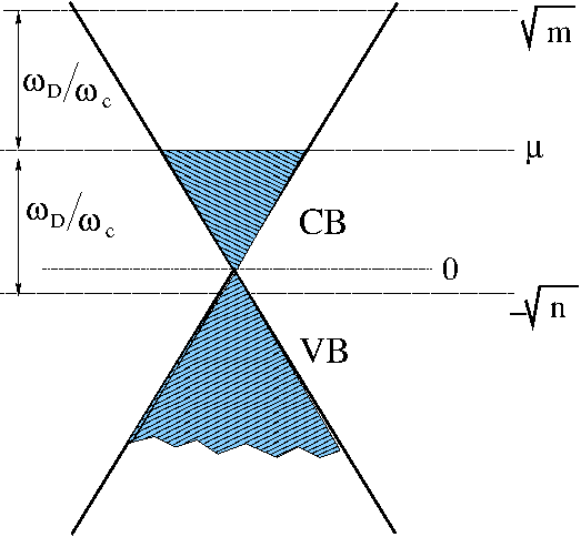
Figure 1: Schematic illustration of the Weyl model bands structure for a positive chemical potential, smaller than the cutoff energy, showing a pair of Landau levels in both subbands at the cutoff energy measured from the Fermi energy.

III Comparison with the standard (nonrelativistic) electron gas model: The semiclassical approximation

A useful reference model, for comparison with the 2D Weyl model developed above, starts with a nonrelativistic electron gas, characterized by a quadratic single-electron energy-momentum dispersion, $E=\frac{\hbar^{2}k^{2}}{2m_{S}^{\ast}}$, with band effective mass, $m_{S}^{\ast}$ , set equal to $\frac{1}{2}m_{0}^{\ast}=\frac{E_{F0}}{2v^{2}}$, and $E_{F0}$- the Fermi energy in the Weyl model at a certain doping level, to be determined in reference to a concrete experiment. Under these assumptions both the Fermi energy, $E_{F0}$ , and the Fermi wave number, $k_{F0}$ , are the same in both models:

$$E_{F0}=\frac{\hbar^{2}k_{F0}^{2}}{2m_{S}^{\ast}}=\hbar vk_{F0}$$ (30)

And in a perpendicular magnetic field $\mathbf{H=}\left(0,0,H\right)$ the cyclotron frequency, $\omega_{c}^{S}\equiv\left(\frac{eH}{m_{S}^{\ast}c}\right)$, is related to the Weyl cyclotron frequency, $\omega_{c}^{W}\equiv\frac{\sqrt{2}v}{a_{H}}$, via:

$$\omega_{c}^{W}=2\sqrt{n_{F0}}\left(\frac{eH}{m_{0}^{\ast}c}\right)=\sqrt{n_{F0}}\omega_{c}^{S}$$ (31)

where in both models

$$n_{F0}\equiv\frac{E_{F0}}{\hbar\omega_{c}^{S}}\equiv\left(\frac{E_{F0}}{\hbar\omega_{c}^{W}}\right)^{2}=\frac{\left(a_{H}k_{F0}\right)^{2}}{2}$$ (32)

Using the set of parameters defined above, the well known expression for the pairing energy eigenvalue obtained in the standard model takes the form:

$$\left|V\right|A_{S}=\frac{1}{4}\lambda_{S}\sum\limits_{m,n=n_{F0}\left(1-\gamma_{0}\right)}^{n_{F0}\left(1+\gamma_{0}\right)}\frac{\left(m+n\right)!}{2^{m+n}n!m!}\frac{\tanh\left(\frac{\mu_{0}-n-1/2}{2\tau_{S}}\right)+\tanh\left(\frac{\mu_{0}-m-1/2}{2\tau_{S}}\right)}{2\mu_{0}-n-m-1}$$ (33)

where $\mu_{0}=n_{F0},\tau_{S}=\frac{k_{B}T}{\hbar\omega_{c}^{S}},\lambda_{S}\equiv\left|V\right|\left(\frac{m_{S}^{\ast}}{2\pi\hbar^{2}}\right)$, and $\gamma_{0}=\hbar\omega_{D}/E_{F0}$.

The semiclassical limit of our theory in the Weyl model is basically established at sufficiently small magnetic fields for which the LL index at the Fermi energy, $n_{F}$, is sufficiently large compared to unity.  Thus, assuming that $n_{F}\gg 1$ , we may expand the CB energy appearing in the dominant contribution to $A$ (i.e. $I_{nm}^{\left(11\right)}$) in Eq.29 around $m=n_{F}$ , or $n=n_{F}$, e.g.: $\ \sqrt{m}\approx\mu+\frac{1}{2\sqrt{n_{F}}}\left(m-n_{F}\right)$, $\sqrt{n}\approx\mu+\frac{1}{2\sqrt{n_{F}}}\left(n-n_{F}\right)$,  such that to leading order: $I_{nm}^{\left(11\right)}\approx 4\sqrt{n_{F}}\frac{\tanh\left(\frac{n_{F}-m}{2\left(2\tau\sqrt{n_{F}}\right)}\right)+\tanh\left(\frac{n_{F}-n}{2\left(2\tau\sqrt{n_{F}}\right)}\right)}{2n_{F}-m-n}$, and:

$$\left|V\right|A_{W}\approx\left|V\right|A_{W}^{SC}=\frac{1}{8}\lambda\sum\limits_{m,n=N_{l}^{\left(1\right)}}^{N_{u}^{\left(1\right)}}\frac{\left(m+n\right)!}{2^{m+n}n!m!}\frac{\tanh\left(\frac{n_{F}-m}{2\left(2\sqrt{n_{F}}\tau_{W}\right)}\right)+\tanh\left(\frac{n_{F}-n}{2\left(2\sqrt{n_{F}}\tau_{W}\right)}\right)}{2n_{F}-m-n}$$ (34)

Note that, for $E_{F}=E_{F0}$, $A_{W}$ in Eq.34 is seen to be close to $\frac{1}{2}A_{S}$ in Eq.33, provided the dimensionless temperature scale $\tau_{W}\equiv\frac{k_{B}T}{\hbar\omega_{c}^{W}}$ is rescaled by the factor $2\sqrt{n_{F0}}$.  In fact, the rescaled value, $2\sqrt{n_{F0}}\tau_{W}=\frac{k_{B}T}{\hbar eH/m_{0}^{\ast}c}=2\left(\frac{k_{B}T}{\hbar\omega_{c}^{S}}\right)=2\tau_{S}$ , is consistent with Eq.31. It should be noted that the dimensionless zero-point energy, $1/2$ in Eq.33, characterizing the standard model, does not make any difference since it can always be absorbed into the chemical potential $\mu$.  The factor of $\frac{1}{2}$ between the expressions 34 and 33 is due to the spin-momentum locking, inherent to the Weyl model, and the consequent splitting of its spectrum into positive and negative energy subbands, as compared to the single band of the standard spectrum.

There is, however, an essential difference between the two models, and that is the cyclotron effective mass in the Weyl model is a function of the Fermi energy, whereas in the standard model it is a constant. The above comparison is, therefore, drastically modified in the ultimate quantum limit, when together with the doping level, the Fermi energy tends to zero, and the prefactor $\frac{\lambda}{\sqrt{n_{F}}}$ in Eq.29 nominally diverges as $n_{F}\rightarrow 0$.  The vanishing of $\lambda$ in the Weyl model with $E_{F}$ through the cyclotron effective mass, evidently removes this divergency, yielding: $\frac{\lambda}{\sqrt{n_{F}}}\rightarrow\frac{1}{\sqrt{2}\pi}\frac{\left|V\right|/\hbar v}{a_{H}},E_{F}\rightarrow 0$ .

It will be, therefore, helpful to extend the reference model expressed in Eq.33 for varying values of $E_{F}$, to account for the dependence of the parameters $n_{F}$ and $m^{\ast}$ in the Weyl model on $E_{F}$.  This can be done by replacing $n_{F0}=\mu_{0}$ in Eq.33 with $n_{F}$, defined in the Weyl model by:

$$n_{F}\equiv\left(\frac{E_{F}}{\hbar\omega_{c}^{W}}\right)^{2}=\frac{1}{2}\left(a_{H}k_{F}\right)^{2}$$ (35)

so that:

$$\left|V\right|A_{S}\rightarrow\frac{1}{4}\lambda_{S}\sum\limits_{m,n=n_{F}\left(1-\gamma\right)}^{n_{F}\left(1+\gamma\right)}\frac{\left(m+n\right)!}{2^{m+n}n!m!}\frac{\tanh\left(\frac{n_{F}-n-1/2}{2\tau_{S}}\right)+\tanh\left(\frac{n_{F}-m-1/2}{2\tau_{S}}\right)}{2n_{F}-n-m-1}$$ (36)

where  $\tau_{S}=\sqrt{n_{F0}}\tau_{W}$ and $\gamma=\hbar\omega_{D}/E_{F}$.    The standard coupling constant, $\lambda_{S}$ , is defined by fixing the value of the cyclotron mass at $m_{S}^{\ast}$ (i.e. at a certain value of the Fermi energy $E_{F0}$): $\lambda_{S}\equiv\left|V\right|\left(m_{S}^{\ast}/2\pi\hbar^{2}\right)=\frac{1}{2}\lambda_{0}$, so that the prefactor in Eq.29 is rewritten in a form showing its independence of $E_{F}$:

$$\frac{\lambda}{\sqrt{n_{F}}}=\frac{\lambda_{0}}{\sqrt{n_{F0}}}=2\frac{\lambda_{S}}{\sqrt{n_{F0}}}$$ (37)

Using this expression in Eq.29, together with the semiclassical approximation that yields Expression 34, the pre-factor, $\lambda/8$, in the latter becomes: $\left(\lambda_{S}/4\right)\left(\frac{k_{F}}{k_{F0}}\right)$, in full agreement with Eq.36 at the reference point $k_{F}=k_{F0}$. For doping levels away from the reference point, i.e. for $k_{F}\neq k_{F0}$, one finds the simple relation:

$$A_{W}^{SC}=\left(\frac{k_{F}}{k_{F0}}\right)A_{S}$$ (38)

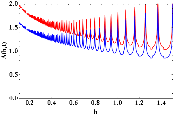
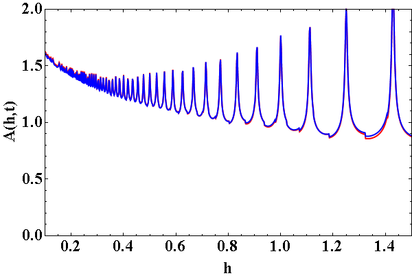
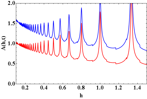
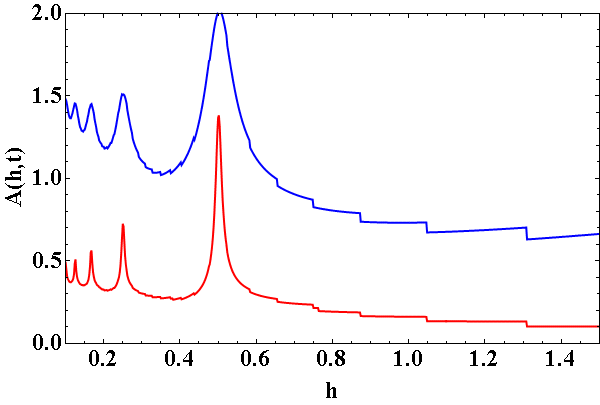
Figure 2: Pairing condensation energy eigenvalue, $A$, as a function of field, $h\equiv H/H_{0}$ , at temperature $t\equiv T/T_{0}=0.01$, calculated for the Weyl model, Eq.29 (red curves), and for the extended standard model, Eq.36 (blue curves), at various values of $\widetilde{n}_{F\text{ }}$($=15$ (a),$10$ (b), $5$ (c), $0.5$ (d)). The reference parameters, $H_{0},T_{0}$ , were selected in accord with the experiment, as discussed in the text. The cutoff was selected at: $\hbar\omega_{D}/E_{F0}=0.5$. Note that for $\widetilde{n}_{F\text{ }}<5$ the cutoff energy $\hbar\omega_{D}>E_{F}$.

IV Mapping between the two models and their comparison with experiment

Experimental evidence for the existence of strong type-II superconductivity in a surface state of a topological insulator under a strong magnetic field can be found in results of transport, magnetic susceptibility, de Haas van Alphen (dHvA) oscillations and scanning tunnelling spectroscopy measurements, reported recently on Sb₂Te₃ Zhao15 . Using a simple s-wave BCS model, similar to the standard model described in Sec.3, with the experimentally observed dHvA frequency, $F_{0}=36.5$ T (implying $n_{F0}\left(H\right)=\frac{F_{0}}{H}$), and cyclotron mass $m_{0}^{\ast}=0.065m_{e}$, it was shown in ZDMPRB17 that such an unusual SC state can exist only in the strong coupling superconductor limit. In particular, the zero field limit of the self-consistent order parameter amplitude, $\Delta_{SC}\left(n_{F0}\rightarrow\infty\right)\rightarrow\hbar\omega_{D}/\sinh\left(1/\lambda_{0}\right)$, calculated in ZDMPRB17 , was found, for $\lambda_{0}=1$ and $\hbar\omega_{D}=0.25E_{F0}$, to basically agree with the spatially average SC energy gap, derived from the STS measurements (i.e. $\simeq 13$ meV) Zhao15 , whereas the LL filling factor, calculated at the semiclassical $H_{c2}$ ( $n_{F0}\approx 14$), was found to agree with the experimentally determined field of the resistivity onset downshift $H_{R}$ ($\sim 2.5$ T, $n_{F0}\sim 14$) Zhao15 .

Such an agreement, between the standard model, outlined in Sec.3, and the experiment reported in Zhao15 , seems to imply that the peculiar features of the helical surface state bands structure distinguishing the 2D Weyl Fermion gas model from the standard model, are irrelevant in constructing its high-fields SC state, except for a single parameter:- its unusual cyclotron effective mass, which can be dramatically modified upon variation of the chemical potential (e.g. by doping or by changing the gate voltage). The analysis presented in Sec.3 supports this conclusion for carrier densities and magnetic fields in the semiclassical limit.

Here we study the relationships between the Weyl model and the extended standard model, described above, in the general parameters range, finding conditions for a complete mapping between the two models, and searching for physical situations in which they are qualitatively distinguishable. In Fig.2 we plot results of the pairing eigenvalue $A$, calculated within both the Weyl and the extended standard models, as a function of the reduced magnetic field, $h\equiv H/H_{0}$, for various values of Fermi energy $E_{F}$.  The temperature was selected sufficiently small to unfold the quantum oscillations associated with the Landau quantization.

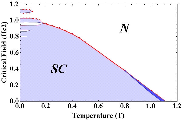
Figure 3: H-T Phase diagram, obtained by solving the self-consistency equation for both models at the reference point: $\widetilde{n}_{F}=\widetilde{n}_{F0}=10$, on the basis of the reference parameters $H_{0},T_{0}$ , as discussed in the text.The cutoff was selected at: $\hbar\omega_{D}/E_{F0}=0.5$. Deviations are seen only around the dark blue area, where the Weyl phase boundary is slightly above the standard one.  Mutual reentrances of the SC and N phases, due to strong magneto-oscillations effect, are seen around the upper-left corner of the phase diagram.

Selecting for the reference parameters the values extracted from the transport and magneto-oscillations measurements Zhao15 , as described above: $F_{0}=36.5T,H_{0}=2.5T$, $m_{0}^{\ast}=0.065m_{e}$, and from the magnetic susceptibility measurements Zhao15 the value: $T_{0}=100K$, we define the dimensionless reference parameters: $\widetilde{\tau}_{S}\equiv\left(k_{B}T_{0}/\hbar\widetilde{\omega}_{c}^{S}\right)$ and $\widetilde{\tau}_{W}\equiv\left(k_{B}T_{0}/\hbar\widetilde{\omega}_{c}^{W}\right)$, where $\widetilde{\omega}_{c}^{S}\equiv\left(eH_{0}/m_{S}^{\ast}c\right)$ and $\widetilde{\omega}_{c}^{W}\equiv\left(\sqrt{2}v/a_{H_{0}}\right)$, so that: $\tau_{S}=\widetilde{\tau}_{S}\left(t/h\right)$ and $\tau_{W}=\widetilde{\tau}_{W}\left(t/\sqrt{h}\right)$.  The two scales are therefore related via: $\widetilde{\tau}_{S}=\left(\widetilde{n}_{F0}\right)^{1/2}\widetilde{\tau}_{W}$ , where $\widetilde{n}_{F0}\equiv\left(a_{H_{0}}k_{F0}\right)^{2}/2\approx 10$.

The eigenvalues $A_{W},A_{S}$, plotted in Fig.2 as functions of $h$, for various values of $\widetilde{n}_{F}\equiv\left(a_{H_{0}}k_{F}\right)^{2}/2$, show at $\widetilde{n}_{F}=\widetilde{n}_{F0}$ complete agreement between the two models, including the fine structure of the quantum oscillations, provided $\widetilde{\tau}_{S}$ is re-scaled to $2\times\left(\widetilde{n}_{F0}\right)^{1/2}\widetilde{\tau}_{W}$, as found in the semiclassical approximation, Eq.34. Under these conditions, solutions of the self consistency equation, $1=\left|V\right|A$, for both models, yield nearly identical results for the H-T phase diagrams, as shown in Fig.3, except for a small deviation in the low fields region, due to the different ultraviolet divergency predicted by the two models. The two intersection points of the phase boundary with the axes, shown in Fig.3, are seen to be close to $t=1$ and $h=1$, thus indicating that the calculated $H_{c2}\left(T\rightarrow 0\right)$ and $T_{c}\left(H\rightarrow 0\right)$ values are close to the values of $H_{0}$ and $T_{0}$, respectively.

For values of $\widetilde{n}_{F}$ away from $\widetilde{n}_{F0}$ the baseline of $A_{W}$ is shifted with respect to that of $A_{S}$, depending on wether $\widetilde{n}_{F}>\widetilde{n}_{F0}$ (shift up), or $\widetilde{n}_{F}<\widetilde{n}_{F0}$ (shift down), thus reflecting the dependence of the pairing correlation in the Weyl model on the carrier density. This behavior is consistent with the relation 38 derived in the semiclassical limit. The oscillatory patterns remain nearly the same, except for slight relative narrowing of the Weyl peaks upon decreasing $\widetilde{n}_{F}$, which becomes quite significant in the quantum limit, e.g. at $\widetilde{n}_{F}=0.5$ in Fig.2d. It is also remarkable that in the ultimate quantum limit, i.e. when $\widetilde{n}_{F}\rightarrow 0$, the pairing correlation in the Weyl model, despite its vanishing normal electron density of states at the Fermi energy, does not vanish.

V Conclusion

In this paper we have developed a Nambu-Gorkov Green’s function approach to strongly type-II superconductivity in a 2D spin-momentum locked (Weyl) Fermi gas model at high perpendicular magnetic fields in order to study the transition to high field surface superconductivity observed recently on the topological insulator Sb₂Te₃Zhao15 . We have found that, for LL filling factors larger than unity, superconductivity in such a 2D Weyl Fermion gas can be mapped onto the standard 2D electron (or hole) gas model, having the same Fermi surface parameters, but with a cyclotron effective mass, $m^{\ast}=E_{F}/2v^{2}$ , which could be dramatically reduced below the free electron mass, $m_{e}$, by manipulating the doping level, or the gate voltage.  Our calculations for Sb₂Te₃ show that the SC helical surface state reported in Zhao15 was in the moderate semiclassical range ($n_{F}\geq 10$), so justifying the mapping with the standard model. They reveal a very unusual, strong type-II superconductivity at low carrier density and small cyclotron effective mass, $m^{\ast}={0.065}m_{e}$, which can be realized only in the strong coupling ($\lambda\sim 1$) superconductor limitZDMPRB17 . Further reduction of the carrier density in such a system could yield an effective cyclotron energy comparable to or larger than the Fermi energy, LL filling factors smaller than unity, and cutoff energy larger than the chemical potential, resulting in significant deviations from the predictions of the standard model.

Note, however, that for such a dilute fermion gas system the simple mean field BCS theoretical framework of superconductivity, exploited in this paper, should be drastically revised, particularly due to the neglect of both phase and amplitude fluctuations of the SC order parameter Emery-Kivel-Nat95 , and to the breakdown of the adiabatic approximation in the electron phonon system GorkovPRB16 . Several recent reports on superconductivity in very dilute fermion gas systems, such as that found in compensated semimetallic FeSe KasaharaNCom16 , or in the large-gap semiconductor SrTiO₃ EdgePRL15 , have drawn much attention to fluctuation superconductivity beyond the Gaussian approximation, which could lead to crossover between weak-coupling BCS and strong-coupling Bose-Einstein condensate limits RanderiaBCS-BEC14 . In the presence of strong magnetic fields the situation is further complicated due to complex interplay between vortex and SC amplitude fluctuations ManivPRB06 .

References

(1) Ivan Bozovic and Charles Ahn, ”A new frontier for
superconductivity”, nphys. 10, 893 (2014).
(2) Jian-Feng Ge et al., ”Superconductivity above 100 K
in single-layer FeSe films on doped SrTiO3”, nmat. 14, 285
(2015).
(3) S. Manna et al., ”Evidence for interfacial
superconductivity in a bi-collinear antiferromagnetically ordered FeTe
monolayer on a topological insulator”, arXiv: 1606.03249 [cond-mat.supr-con].
(4) T. Maniv, V. Zhuravlev, I. D. Vagner, and P. Wyder,”Vortex
states and quantum magnetic oscillations in conventional type-II
superconductors”, Rev. Mod. Phys. 73, 867 (2001).
(5) Lukas Zhao, Haiming Deng, Inna Korzhovska, Milan
Begliarbekov, Zhiyi Chen, Erick Andrade, Ethan Rosenthal, Abhay Pasupathy,
Vadim Oganesyan & Lia Krusin-Elbaum, ”Emergent surface superconductivity
in the topological insulator Sb2Te3”, nature communications DOI:
10.1038/ncomms9279 (2015).
(6) Haijun Zhang, Chao-Xing Liu, Xiao-Liang Qi, Xi Dai, Zhong
Fang and Shou-Cheng Zhang, ”Topological insulators in Bi2Se3,
Bi2Te3 and Sb2Te3 with a single Dirac cone on
the surface”, nphys. 5 , 438 (2009).
(7) M. I. Katsnelson, ”Graphen, Carbon in two
Dimensions”, Cambridge University Press, Cambridge (2012).
(8) F. Arnold, M. Naumann, S.-C. Wu, Y. Sun, M. Schmidt, H.
Borrmann, C. Felser, B. Yan, and E. Hassinger, ”Chiral Weyl Pockets and
Fermi Surface Topology of the Weyl Semimetal TaAs”, Phys. Rev. Lett. 117, 146401 (2016).
(9) V. Zhuravlev, W. Duan, and T. Maniv, ”Self-consistent
Bogoliubov–de Gennes theory of the vortex lattice state in a
two-dimensional strongly type-II superconductor at high magnetic fields”,
Phys. Rev. B 95, 024502 (2017).
(10) G. Tkachov, ”Topological Insulators, The Physics of Spin
Helicity in Quantum Transport”, San Stanford Publ. Singapore 038988 (2016).
(11) E. Helfand, and N. R. Werthamer, Phys. Rev. Lett. 13, 686 (1964); Phys. Rev. 147, 288 (1966).
(12) Note that the Hamiltonian in Eq.3, with a
spin-singlet , can also yield spin-triplet
pairing correlation, due to the spin-momentum locking term , which breaks the spin-rotation symmetry, as was first shown by L.
Fu and C. I. Kane, in Phys. Rev. Lett., 100, 096407 (2008) (see
also Tkachov16 ). However, a self-consistent triplet order parameter
requires also spin dependent pair coupling (e.g. via electronic exchange
interaction).
(13) V. J. Emery and S. A. Kivelson, ”Importance of
phase fluctuations in superconductors with small superfluid density”, Nature
374 , 434 (1995).
(14) L. P. Gor’kov, ”Superconducting transition
temperature: Interacting Fermi gas and phonon mechanisms in the nonadiabatic
regime”, Phys. Rev. B 93, 054517 (2016).
(15) S Kasahara, T Yamashita, A Shi, R Kobayashi, Y
Shimoyama, T Watashige, K Ishida, T Terashima, T Wolf, F Hardy, C Meingast,
H V Lőhneysen, A Levchenko, T Shibauchi, Y Matsuda, ”Giant
Superconducting Fluctuations in the Compensated Semimetal FeSe at the
BCS–BEC Crossover”, Nature Commun. 7, 12843 (2016).
(16) J. M. Edge, Y. Kedem, U. Aschauer, N. A. Spaldin, and A.
V. Balatsky, ”Quantum Critical Origin of the Superconducting Dome in SrTiO3”, Phys. Rev. Lett. 115, 247002 (2015). Erratum Phys. Rev.
Lett. 117, 219901 (2016).
(17) M. Randeria, and E. Taylor, ”Crossover from
Bardeen-Cooper-Schrieffer to Bose-Einstein condensation and the unitary
Fermi gas”, Annu. Rev. Condens. Matter Phys. 5, 209–232 (2014).
(18) T. Maniv, V. Zhuravlev, J. Wosnitza, O. Ignatchik, B.
Bergk, and P. C. Canfield, ”Broadening of the superconducting transition by
fluctuations in three-dimensional metals at high magnetic fields”, Phys.
Rev. B 73, 134521 (2006).