A multiplicative coalescent with asynchronous multiple mergers

Abstract

We define a Markov process on the partitions of $[n]=\{1,\ldots,n\}$ by drawing a sample in $[n]$ at each time of a Poisson process, by merging blocks that contain one of these points and by leaving all other blocks unchanged. This coalescent process appears in the study of the connected components of random graph processes in which connected subgraphs are added over time with probabilities that depend only on their size.
First, we determine the asymptotic distribution of the coalescent time. Then, we define a Bienaymé-Galton-Watson (BGW) process such that its total population size dominates the block size of an element. We compute a bound for the distance between the total population size distribution and the block size distribution at a time proportional to $n$. As a first application of this result, we establish the coagulation equations associated with this coalescent process. As a second application, we estimate the size of the largest block in the subcritical and supercritical regimes as well as in the critical window.

Keywords. Coalescent process, Poisson point process, branching process, random graph process, coagulation equations.
AMS MSC 2000. Primary 60C05. Secondary 05C80, 60J80, 60K35.

Introduction

The paper is devoted to studying a family of multiplicative coalescent processes on a finite set $S$ defined by a simple algorithm. To present this algorithm, let us fix a probability distribution $p$ on $\operatorname{\mathbb{N}}^{*}$. We construct a coalescent process denoted $(\Pi_{S,p}(t))_{t\geq 0}$ by the following algorithm:

1. $\Pi_{S,p}(0)$ is the partition defined by the singletons of $S$;

2. At each event $\tau$ of a Poisson process $(Z_{t})_{t}$ with intensity one, we choose a positive integer $k$ according to $p$ and we draw $k$ elements $x_{1},\ldots,x_{k}$ in $S$ by a simple random sampling with replacement. The partition at time $\tau$ is defined by merging blocks of $\Pi_{S,p}(\tau^{-})$ that contain $x_{1},\ldots,x_{k}$ into one block and by leaving all other blocks unchanged.

By construction, only one merger can occur at a given time but it may involve more than two blocks. The probability that blocks coalesce depends only on the product of their sizes. Such a coalescent process naturally appears when considering a random hypergraph process on the set of vertices $S$ of size $|S|=n$.

A random hypergraph process can be defined as a Markov process $(\mathcal{G}(t))_{t\geq 0}$ whose states are hypergraphs on $S$: it starts with the empty graph and hyperedges (i.e. subsets of $S$) are added over time according to a given rule. There are several possible definitions of hypergraph components. One way is to identify a hyperedge $A$ to a connected subgraph and then a hypergraph to a multigraph; the component of a vertex can be defined as usual in a graph. The process defined by the connected components of $\mathcal{G}(t)$ for $t\geq 0$ is a coalescent process. Here are two examples of classical random hypergraph processes.

• Erdös-Rényi random graph. If a pair, chosen with a uniform distribution on $S^{2}$, is added at each time of a Poisson process with intensity one, we obtain a variant of the Erdös-Rényi random graph process denoted $(\mathcal{H}(n,t))_{t\geq 0}$: the probability that ${e=(i,j)\in S^{2}}$ is an edge of $\mathcal{H}(n,t)$ is equal to $1-\exp(-\frac{2t}{n^{2}})$ and the coalescent process associated with $(\mathcal{H}(n,t))_{t\geq 0}$ has the same distribution as $(\Pi_{S,p}(t))_{t\geq 0}$ where $p$ is the Dirac measure on $2$ and $|S|=n$.

• Uniform random graph process. For a fixed $d>2$, if a subset of size $d$ chosen with a uniform distribution on $S^{d}$, is added at each time of a Poisson process with intensity one, it defines a random hypergraph process whose components have similar properties as a $d$-uniform random graph process. The partition defined by the connected components of this random hypergraph process has the same law as $(\Pi_{S,p}(t))_{t\geq 0}$ where $p$ is the Dirac measure on $d$.

More generally, if each new hyperedge $A$ added is chosen with a distribution $\nu$ that depends only on the number of vertices in $|A|$, then the associated coalescent process has the same distribution as $(\Pi_{S,p}(t))_{t}$, where $p(|A|)=\nu(A)$ for every $A\subset S$.

Let us present the properties of $\mathcal{H}(n,\frac{nt}{2})$ which are related to our study. For each property, we shall also review works done on random hypergraphs to introduce our contribution. Precise statements of our results will be described in Section 2.

1. Connectivity threshold
   Erdös and Rényi in [12] and independently Gilbert in [17] have studied the probability that the random graph models they introduced are connected. Erdös and Rényi results can be formulated for the random graph process $(\mathcal{H}(n,\frac{nt}{2}))_{t}$ as follows:

   Theorem.

   For every $c\in\operatorname{\mathbb{R}}$ and every $k\in\operatorname{\mathbb{N}}$, the probability that $\mathcal{H}(n,\frac{n}{2}(\log(n)+c))$ contains a connected component of size $n-k$ and $k$ isolated points converges to $\displaystyle{\exp(-e^{-c})\frac{e^{-ck}}{k!}}$ as $n\rightarrow$ tends to $+\infty$.

   This shows that $\frac{n}{2}\log(n)$ is a sharp threshold function for the connectivity property.

   Poole in his thesis [35], has extended this result for uniform random hypergraphs: the threshold for connectivity of a $d$-uniform random hypergraph is $\frac{n}{d}\log(n)$ for every $d\geq 2$. Kordecki in [23] has given a general formula for the probability that a random hypergraph is connected for non-uniform random hypergraph with bounded hyperedges.

   Poisson point processes of Markov loops on a finite graph give examples of random graph processes for which connected subgraphs (close walks here) are added over time (see [25] and [24] for a survey of their properties). Some general properties of the coalescent process induced by them have been presented by Le Jan and the author in [26]. In particular, it has been shown that when loops are constructed by a random walk killed at a constant rate on the complete graph $K_{n}$, the coalescent process associated with the Poissonian ensembles of loops can be constructed as $\Pi_{S,p}$, where $p$ is a logarithmic distribution with a parameter depending on the killing rate; the connectivity threshold function have been established.

   By a similar study, we extend the statement of the previous theorem for a large class of distributions for $p$ that contains probability distributions having a finite moment of order two showing in particular that the connectivity threshold for a random hypergraph whose components are described by $\Pi_{S,p}$ is $\displaystyle{\frac{|S|\log(|S|)}{\sum_{k\geq 2}kp(k)}}$ (Theorem Theorem).

2. Phase transition.
   The largest block size of $\mathcal{H}(n,\frac{nt}{2})$ undergoes a phase transition. It was first proved by Erdös and Rényi in [13]. The statement we present is taken from [42], where the proof is based on the use of Bienaymé-Galton-Watson (BGW) processes.

   Theorem ([42]).

   Let $c^{(n)}_{t}(x)$ denote the component size of a vertex $x$ of $\mathcal{H}(n,\frac{nt}{2})$ and let $c^{(n)}_{1,t}\geq c^{(n)}_{2,t}$ denote the two largest component sizes.

   1. Assume that $t<1$.

      • For every vertex $x$, $c^{(n)}_{t}(x)$ converges in distribution to the total population size of a BGW process with one progenitor and Poisson($t$) offspring distribution.

      • Let $I_{t}$ be the value at 1 of the Cramér function of the Poisson$(t)$-distribution: $I_{t}=t-1-\log(t)$.
        The sequence $\displaystyle{\left(\frac{c^{(n)}_{1,t}}{\log(n)}\right)_{n}}$ converges in probability to $1/I_{t}$.

   2. Assume that $t>1$ and denote by $q_{t}$ the extinction probability of a BGW process with one progenitor and Poisson($t$) offspring distribution.
      For every $a\in]1/2,1[$, there exist $b>0$ and $c>0$ such that

      $$\operatorname{\mathbb{P}}(|c^{(n)}_{1,t}-(1-q_{t})n|\geq n^{a})+\operatorname{\mathbb{P}}(c^{(n)}_{2,t}\geq c\log(n))=O(n^{-b}).$$

   3. Assume that $t=1+\theta n^{-1/3}$ for some $\theta\in\operatorname{\mathbb{R}}$. There exists a constant $b(\theta)>0$ such that for every $w>1$ and every $n\in\operatorname{\mathbb{N}}^{*}$,

      $$\operatorname{\mathbb{P}}(c^{(n)}_{1,1+\theta n^{-1/3}}>wn^{2/3})\leq\frac{w}{b(\theta)}\;\text{and}\;\operatorname{\mathbb{P}}(c^{(n)}_{1,1+\theta n^{-1/3}}<w^{-1}n^{2/3})\leq\frac{w}{b(\theta)}.$$

   In [40], Schmidt-Pruzan and Shamir studied the size of the largest component for non-uniform random hypergraphs: in their model, the size of hyperedges is bounded and the probability that the hypergraph has a fixed hyperedge depends only on the size of the hyperedge. They established similar statements for the largest component when the average degree of a vertex in the hypergraph is less than 1, equal to 1 and greater than 1. More precise results on the phase transition have been established later in the case of uniform random hypergraphs (see [21]). Bollobás, Janson and Riordan in [5] have studied the size of the connected components for a general model of random hypergraph: in their model a type is associated with each vertex and the probability to add a hyperedge $A$ depends on the types of the elements in $A$. From their study we can deduce that the size of the largest block of $\Pi_{S,p}(|S|t)$ is $o_{p}(|S|)$ if $t\sum_{k\geq 2}k(k-1)p(k)<1$ and $\rho|S|+o_{p}(|S|)$ if $t\sum_{k\geq 2}k(k-1)p(k)>1$, where $1-\rho$ is the smallest positive solution of the following equation:

   $$x=\exp\left(-t\sum_{k\geq 2}kp(k)(1-x^{k-1})\right).$$

   ($\rho$ can be seen as the survival probability of a BGW process with a compound Poisson offspring distribution). Janson in [20] proved a conjecture proposed by Durrett in [9] saying that for a random graph with a power law degree distribution with exponent $\gamma>3$, the largest component in the subcritical phase is of order $n^{\frac{1}{\gamma-1}}$. This result suggests that the size of the largest block of $\Pi_{S,p}(|S|t)$ in the subcritical phase would be also order $|S|^{\alpha}$ for some $0<\alpha$ if $p$ does not have all its power moments finite.

   Under the assumption that $p$ has a finite third moment, we give a bound for the distance between the cumulative distributions of the block size of an element and of the total population size of a BGW process with compound Poisson offspring distribution (Theorem 2.3). We deduce from this the asymptotic distribution of two block size as $|S|$ tends to $+\infty$ (Corollary 2.8). We also study the largest block size in three different regimes (Theorems 2.12 and 2.14): in the subcritical phase, we show that the size of the largest block is $\displaystyle{o_{p}(|S|^{\frac{1+\varepsilon}{u-1}})}$ for every $\varepsilon>0$, if $p$ has a finite moment of order $u\geq 3$ and is $O_{p}(\log(|S|))$, if $p$ is a light-tailed distribution. When $p$ is a regularly varying distribution with index smaller than $-3$, we also establish that the size of the largest block grows faster than a positive power of $|S|$ as $|S|$ tends to $+\infty$. In the critical window, we show that the size of the largest block is $O_{p}(n^{2/3})$. Although the supercritical regime is studied in [5], to complete the analysis of the largest block we present a simple proof of the property stated in (b) for our model.

3. Hydrodynamic behavior
   Let us now consider the average number of components of size $x$ in $\mathcal{H}(n,\frac{nt}{2})$.

   • For any $t>0$ and $x\in\operatorname{\mathbb{N}}^{*}$, the average number of components of size $x$ in $\mathcal{H}(n,\frac{nt}{2})$ converges in $L^{2}$ to

     $$v(x,t)=\frac{(tx)^{x-1}e^{-tx}}{x.x!}.$$

     The value $xv(x,t)$ is equal to the probability that $x$ is the total population size of a BGW process with one progenitor and Poisson($t$) offspring distribution.

   • $\{v(x,\cdot),\ x\in\operatorname{\mathbb{N}}^{*}\}$ is the solution on $\operatorname{\mathbb{R}}_{+}$ of the Flory’s coagulation equations with multiplicative kernel:

     $$\frac{d}{dt}v(x,t)=\frac{1}{2}\sum_{y=1}^{x-1}y(x-y)v(y,t)v(x-y,t)\\ -\sum_{y=1}^{+\infty}xyv(x,t)v(y,t)-xv(x,t)\sum_{y=1}^{+\infty}y\big{(}v(y,0)-v(y,t)\big{)}$$ (0.1)

     Up to time 1, this solution coincides with the solution of the Smoluchowski’s coagulation equations with multiplicative kernel starting from the monodisperse state:

     $$\frac{d}{dt}v(x,t)=\frac{1}{2}\sum_{y=1}^{x-1}y(x-y)v(y,t)v(x-y,t)-xv(x,t)\sum_{y=1}^{+\infty}yv(y,t).$$ (0.2)

     Equations (0.2) introduced by Smoluchowski in [41] are used for example to describe aggregations of polymers in an homogeneous medium where diffusion effects are ignored. The first term in the right-hand side describes the formation of a particle of mass $x$ by aggregation of two particles, the second sum describes the ways a particle of mass $x$ can be aggregated with another particle. If the total mass of particles decreases after a finite time, the system is said to exhibit a ‘phase transition’ called ‘gelation’: the loss of mass is interpreted as the formation of infinite mass particles called gel. Smoluchowski’s equations do not take into account interactions between gel and finite mass particles. Equations (0.1) introduced by Flory in [14] are a modified version of the Smoluchowski’s equations with an extra term describing the loss of a particle of mass $x$ by ‘absorption’ in the gel. Let $T_{gel}$ denote the largest time such that the Smoluchowski’s coagulation equations with monodisperse initial condition have a solution which has the mass-conserving property. Then, $T_{gel}=1$ and $T_{gel}$ coincides with the smallest time when the second moment $\sum_{x=1}^{+\infty}x^{2}v(x,t)$ diverges (see [30]). Let us note that the random graph process $(\mathcal{H}(n,\frac{nt}{2}))_{t\geq 0}$ is equivalent to the microscopic model introduced by Marcus [28] and further studied by Lushnikov [27] (see [7] for a first study of the relationship between these two models and [1] for a review, [33], [32] and [16] for convergence results of Marcus-Lushnikov’s model to (0.1)).

   Recently, Riordan and Warnke in [38] gave sufficient conditions under which the average number of blocks of size $x$ converges for a class of random graph processes in which a bounded number of edges can be added at each step according to a fixed rule. This class includes uniform random hypergraph processes. As far as we know such a result has not been established for more general random hypergraph processes.

   Under the assumption that $p$ has a finite third moment, we show that the average number of blocks of size $x$ in the coalescent process $\Pi_{S,p}$ converges in $L^{2}$ to the solution of coagulation equations in which more than two particles can collide at the same time at a rate that depends on the product of their masses (Theorem 2.9).

Remark. Let us note that Darling, Levin and Norris have introduced in [8] a random hypergraph model called Poisson$(\rho)$ random hypergraph process and denoted $(\Lambda_{t})_{t\geq 0}$. The process $(\Lambda_{t})_{t\geq 0}$ is defined as follows:

• Start with the set of vertices $S$;

• At each event $\tau$ of a Poisson process with intensity $1$, choose a positive integer $k\leq|S|$ with probability $\rho(k)$ and a subset $A$ uniformly at random from the subsets of $S$ of size $k$. Then, add $A$ in the hyperedges subset of $\Lambda_{\tau^{-}}$.

One can choose $\rho$ so that the coalescent process defined by the connected components of $(\Lambda_{t})_{t\geq 0}$ is described by $\Pi_{S,p}$. Indeed, $p(k)$ in the definition of $\Pi_{S,p}$ describes the probability to add a subset defined by $k$ elements of $S$ chosen by a simple random sampling with replacement. Hence, if we set

$$\rho(j)=\frac{\binom{|S|}{j}}{|S|}\sum_{k=j}^{+\infty}\frac{p(k)}{|S|^{k}}\sum_{\begin{subarray}{c}(k_{1},\ldots,k_{j})\in(\operatorname{\mathbb{N}}^{*})^{j},\\ k_{1}+\cdots+k_{j}=k\end{subarray}}\binom{k}{k_{1},\ldots,k_{|A|}}\;\text{for every}\;1\leq j\leq|S|,$$

then $\Pi_{S,p}$ is the coalescent process defined by the connected components of $(\Lambda_{t})_{t\geq 0}$. In [8], the object of study is not the connected components of $(\Lambda_{t})_{t\geq 0}$ as we have defined them in our study but identifiable vertices.

Organization of the paper. Section 1 is devoted to a presentation of general properties of the coalescent process we study. The main results are stated in Section 2. In Section 3, we first study the distribution of the number of singletons in the coalescent process and the first time $\tau^{(singl)}_{n}$ the coalescent $\Pi_{\llbracket{n}\rrbracket,p}$ does not have singleton. Next we show that the distribution of the coalescent time $\tau^{(coal)}_{n}$ coincides with the asymptotic distribution of $\tau^{(singl)}_{n}$ as $n$ tends to $+\infty$ which proves Theorem 2.1. In Section 4, we describe the exploration process used to compute the block size of an element and to construct the associated BGW process. The asymptotic distribution of the block size of an element is studied in Section 5: proofs of Theorem 2.3 and its corollaries are presented. Section 6 is devoted to the proof of Theorem 2.9 that describes the hydrodynamic behaviour of the coalescent process. In Section 7, we prove Theorems 2.12 and 2.14 which present some properties of the largest block size in the subcritical, critical and supercritical regimes. Appendix A contains some properties of BGW processes with a compound Poisson offspring distribution.

1 Description of the model and general properties

To study the properties of $(\Pi_{S,p}(t))_{t>0}$, it is useful to construct it by the mean of a Poisson point process instead of the algorithm presented in the introduction. Let us first introduce some notations associated with a finite set $S$:

• The number of elements of $S$ is denoted by $|S|$.

• $\mathcal{W}(S):=\cup_{k\in\operatorname{\mathbb{N}}^{*}}S^{k}$ denotes the set of nonempty tuples over $S$ and $\mathfrak{P}(S)$ is the set of nonempty subsets of $S$.

• A tuple is called nontrivial if it contains at least two different elements of $S$. We write $\mathcal{W}^{*}(S)$ for the set on nontrivial tuples over $S$.

• The length of a tuple $w\in\mathcal{W}(S)$ is denoted by $\ell(w)$.

1.1 The Poisson sample sets

Let $p=\sum_{i=1}^{+\infty}p(i)\delta_{i}$ be a probability measure on $\operatorname{\mathbb{N}}^{*}$ such that $p(1)<1$. We denote by $G_{p}$ its probability generating function: $G_{p}(s)=\sum_{k=1}^{+\infty}p(k)s^{k}$ for $|s|\leq 1$. The following algorithm ‘Choose an integer $K$ with probability distribution $p$ and sample with replacement $K$ elements of $S$’ defines a probability measure on $\mathcal{W}(S)$ denoted by $\mu_{S,p}$:

$$\mu_{S,p}(\{x\})=\frac{p(\ell(x))}{|S|^{\ell(x)}}\text{ for every }x\in\mathcal{W}(S).$$

We consider a Poisson point process $\mathcal{P}_{S,p}$ with intensity $\text{Leb}\times\mu_{S,p}$ on $\operatorname{\mathbb{R}}_{+}\times\mathcal{W}(S)$ and for $t\geq 0$, we define $\mathcal{P}_{S,p}(t)$ as the projection of the set $\mathcal{P}_{S,p}\cap([0,t]\times\mathcal{W}(S))$ on $\mathcal{W}(S)$: $\mathcal{P}_{S,p}(t)$ corresponds to the set of samples chosen before time $t$.

Remark 1.1.

Let $S^{\prime}$ be a subset of $S$.

1. The conditional probability $\mu_{S,p}(\cdot\mid\mathcal{W}(S^{\prime}))$ seen as a probability on $\mathcal{W}(S^{\prime})$ is equal to $\mu_{S^{\prime},p_{S|S^{\prime}}}$ where $p_{S|S^{\prime}}$ is the probability on $\operatorname{\mathbb{N}}^{*}$ defined by:

   $$p_{S|S^{\prime}}(k)=\Big{(}\frac{|S^{\prime}|}{|S|}\Big{)}^{k}\frac{p(k)}{G_{p}\big{(}\frac{|S^{\prime}|}{|S|}\big{)}}\text{ for every }k\in\operatorname{\mathbb{N}}^{*}.$$

   In particular, the restriction of $\mathcal{P}_{S,p}(t)$ to tuples in $\mathcal{W}(S^{\prime})$ before time $t$ has the same distribution as $\mathcal{P}_{S^{\prime},p_{S|S^{\prime}}}\Big{(}G_{p}\big{(}\frac{|S^{\prime}|}{|S|}\big{)}t\Big{)}$.
   

2. Let us also note that the pushforward measure of $\mu_{S,p}$ by the projection $\pi_{S,S^{\prime}}$ from $\mathcal{W}(S)$ to $\mathcal{W}(S^{\prime})$ is equal to $\mu_{S^{\prime},p^{\{S^{\prime}\}}}$ where $p^{\{S^{\prime}\}}$ is the probability on $\operatorname{\mathbb{N}}^{*}$ defined by:

   $$p^{\{S^{\prime}\}}(k)=\Big{(}\frac{|S^{\prime}|}{|S|}\Big{)}^{k}\sum_{\ell=0}^{+\infty}p(k+\ell)\binom{k+\ell}{k}\Big{(}1-\frac{|S^{\prime}|}{|S|}\Big{)}^{\ell}\text{ for every }k\in\operatorname{\mathbb{N}}^{*}.$$

Remark 1.2.

The order of elements in a tuple $w$ will play no role in the definition of the coalescent process, the main object is the subset of $S$ formed by the elements of $w$. The pushforward measure of $\mu_{S,p}$ on $\mathfrak{P}(S)$ is the probability measure $\bar{\mu}_{S,p}$ defined by

$$\bar{\mu}_{S,p}(\{A\})=\sum_{k=|A|}^{+\infty}\frac{p(k)}{|S|^{k}}\sum_{\begin{subarray}{c}(k_{1},\ldots,k_{|A|})\in(\operatorname{\mathbb{N}}^{*})^{|A|},\\ k_{1}+\cdots+k_{|A|}=k\end{subarray}}\binom{k}{k_{1},\ldots,k_{|A|}}\;\text{for every}\;A\in\mathfrak{P}(S).$$

We choose to work with the Poisson point process on $\operatorname{\mathbb{R}}_{+}\times\mathcal{W}(S)$ instead of the associated Poisson point process on $\operatorname{\mathbb{R}}_{+}\times\mathfrak{P}(S)$ because some proofs are simpler to write.

To shorten the description we use sometimes a tuple $w\in\mathcal{W}(S)$ as the subset formed by its elements and write $x\in w$ for $x\in S$ to mean that $x$ is an element of the tuple $w$ and $w\cap A\neq\emptyset$ for $A\subset S$ to mean that $w$ contains some elements of the subset $A$.

1.2 The coalescent process

If $A$ is a subset of $S$, we define the $\mathcal{P}_{S,p}(t)$-neighborhood of $A$ as follows:

$$\mathcal{V}_{A}(t)=A\cup\{i\in S,\;\exists w\in\mathcal{P}_{S,p}(t)\text{ such that }i\in w\text{ and }w\cap A\neq\emptyset\}.$$

We can iterate this definition by setting: $\mathcal{V}^{k}_{A}(t)=\mathcal{V}^{k-1}_{\mathcal{V}_{A}(t)}(t)$ for $k\in\operatorname{\mathbb{N}}^{*}$.
Given any $(i,j)\in S^{2}$, set $i\underset{t}{\sim}j\text{ if and only if }\exists k\in\operatorname{\mathbb{N}}^{*}\;\text{ such that }j\in\mathcal{V}^{k}_{\{i\}}(t)$. This defines an equivalence relation on $S$. We denote by $\Pi_{S,p}(t)$ the partition of $S$ defined by $\underset{t}{\sim}$. In other words, two elements $i$ and $j$ are in a same block of the partition $\Pi_{S,p}(t)$ if and only if there exists a finite number of tuples $w_{1},w_{2},\ldots,w_{k}\in\mathcal{P}_{S,p}(t)$ such that $i\in w_{1}$, $j\in w_{k}$ and $w_{i}\cap w_{i+1}\neq\emptyset$ for every $1\leq i\leq k-1$.

The evolution in $t$ of $\Pi_{S,p}(t)$ defines a coalescent process on $S$. Let us note that this coalescent process depends only on the restriction of $\mathcal{P}_{S,p}$ to $\operatorname{\mathbb{R}}_{+}\times\mathcal{W}^{*}(S)$.

1.2.1 Transition rates and semigroup of the coalescent process

Let us describe the transition rates and the semigroup of $\Pi_{S,p}$.

Proposition 1.3.

Let $\pi$ be a partition of $S$ into non-empty blocks $\{B_{i},\;i\in I\}$.

1. From state $\pi$, the only possible transitions of $(\Pi_{S,p}(t))_{t\geq 0}$ are to partitions $\pi^{\oplus J}$ obtained by merging blocks, indexed by some subset $J$ of $I$ of size greater than or equal to two, to form one block $B_{J}=\cup_{j\in J}B_{j}$ and leaving all other blocks unchanged. Its transition rate from $\pi$ to $\pi^{\oplus J}$ is equal to:

   $$\tau_{\pi,\pi^{\oplus J}} =\sum_{k\geq|J|}\frac{p(k)}{|S|^{k}}\sum_{\begin{subarray}{c}(k_{1},\ldots,k_{|J|})\in(\operatorname{\mathbb{N}}^{*})^{|J|},\\ k_{1}+\cdots+k_{|J|}=k\end{subarray}}\binom{k}{k_{1},\ldots,k_{|J|}}\prod_{j\in J}|B_{j}|^{k_{j}}$$ (1.1)

   $$=\sum_{H\subset J}(-1)^{|H|}G_{p}\Big{(}\frac{|B_{J\setminus H}|}{|S|}\Big{)}.$$ (1.2)

2. For every partition $\pi_{0}$ of $S$,

   $$\operatorname{\mathbb{P}}(\Pi_{S,p}(t)\text{ is finer than }\pi\mid\Pi_{S,p}(0)=\pi_{0})\\ =\exp\left(-t\left(1-\sum_{i\in I}G_{p}\left(\frac{|B_{i}|}{|S|}\right)\right)\right)\operatorname{\mathds{1}}_{\{\pi_{0}\;\text{is finer than}\;\pi\}}$$ (1.3)

Proof.

1. The transition rate $\tau_{\pi,\pi^{\oplus J}}$ is equal to the $\mu_{S,p}$-measure of tuples $w\in\mathcal{W}(B_{J})$ that contain elements of each block $B_{j}$ for $j\in J$. The first formula is obtained by enumerating such tuples ordered by their length. The inclusion-exclusion formula yields the second formula since

   $$\tau_{\pi,\pi^{\oplus J}}=\mu_{S,p}(\mathcal{W}(B_{J}))-\mu_{S,p}\left(\underset{i\in J}{\cup}\mathcal{W}(B_{J\setminus\{i\}})\right).$$

2. $\Pi_{S,p}(t)$ is finer than $\pi$ if and only if every tuple chosen before time $t$ is included in a block of the partition $\pi$. Therefore, if $\pi_{0}$ is finer than $\pi$,

   $$\operatorname{\mathbb{P}}(\Pi_{S,p}(t)\text{ is finer than }\pi\mid\Pi_{S,p}(0)=\pi_{0})=\exp\Big{(}-t\big{(}\mu_{S,p}(\mathcal{W}(S))-\sum_{i\in I}\mu_{S,p}(\mathcal{W}(B_{i}))\big{)}\Big{)}.$$

∎

Example 1.4.

If $p$ is the Dirac measure $\delta_{\{2\}}$, then the only possible transitions of $(\Pi_{S,p}(t))_{t}$ are from a partition $\pi=(B_{i},\;i\in I)$ to partitions obtained by merging two blocks $B_{i}$ and $B_{j}$; the transition rate for such a transition is: $\displaystyle{\tau_{\pi,\pi^{\oplus\{i,j\}}}=2\frac{|B_{i}||B_{j}|}{|S|^{2}}}$. Therefore, for a partition $\pi$ of $S$ into non-empty blocks $\{B_{i},\;i\in I\}$ coarser than a partition $\pi_{0}$ of $S$,

$$\operatorname{\mathbb{P}}(\Pi_{S,\delta_{\{2\}}}(t)\text{ is finer than }\pi\mid\Pi_{S,\delta_{\{2\}}}(0)=\pi_{0})=\exp\left(-2t\sum_{i,j\in I\text{ s.t. }i<j}\frac{|B_{i}||B_{j}|}{|S|^{2}}\right).$$

Example 1.5.

Let $p$ be the logarithmic distribution with parameter $a\in]0,1[$: $p(k)=c\frac{a^{k}}{k}$ with $\frac{1}{c}=-\log(1-a)$ for every $k\in\operatorname{\mathbb{N}}^{*}$. For a partition $\pi$ of $S$ into non-empty blocks $\{B_{i},\;i\in I\}$ coarser than a partition $\pi_{0}$ of $S$,

$$\operatorname{\mathbb{P}}(\Pi_{S,p}(t)\text{ is finer than }\pi\mid\Pi_{S,p}(0)=\pi_{0})=(1-a)^{ct}\prod_{i\in I}\left(1-a\frac{|B_{i}|}{|S|}\right)^{-ct}.$$ (1.4)

This shows that $\Pi_{S,p}(t)$ has the same distribution as a coalescent process describing the evolution of the clusters of Poissonian loop sets on a complete graph defined in [26].

Let us briefly present how these Poissonian loop sets are defined. Let $S$ stand for the vertices of a finite graph $\mathcal{G}$ with $n$ vertices and let consider a simple random walk on $\mathcal{G}$ killed at each step with probability $1-a$. In other words, $\mathcal{G}$ is endowed with unit conductances and a uniform killing measure with intensity $\kappa_{n}=n(\frac{1}{a}-1)$. A discrete based loop $\ell$ of length $k\in\operatorname{\mathbb{N}}^{*}$ on $\mathcal{G}$ is defined as an element of $\mathcal{G}^{k}$. To each element $\ell=(x_{1},\ldots,x_{k})$ of $\mathcal{G}^{k}$ of length $k\geq 2$ is assigned the weight $\dot{\mu}(\ell)=\frac{1}{k}P_{x_{1},x_{2}}\ldots P_{x_{k},x_{1}}$ where $P$ denotes the transition matrix of the random walk. When $\mathcal{G}$ is the complete graph $K_{n}$ then $\dot{\mu}(\ell)=\frac{a^{k}}{kn^{k}}$ for every $\ell\in K_{n}^{k}$. A based loop $\ell=(x_{1},\ldots,x_{k})$ is said to be equivalent to the based loop $(x_{i},\ldots,x_{k},x_{1},\ldots,x_{i-1})$ for every $i\in\{2,\ldots,k\}$. An equivalent class of based loops is called a loop. Let $\mathcal{DL}(\mathcal{G})$ denote the set of loops on $\mathcal{G}$. The measure $\dot{\mu}$ on the set of based loops of length at least two induces a measure on loops denoted by $\mu$. The Poisson loop sets on $\mathcal{G}$ is defined as a Poisson point process $\mathcal{DP}$ with intensity $\text{Leb}\times\mu$ on $\operatorname{\mathbb{R}}_{+}\otimes\mathcal{DL}(\mathcal{G})$. For $t>0$, let $\mathcal{DL}^{(n)}_{t}$ be the projection of the set $\mathcal{DP}\cap([0,t]\times\mathcal{DL}(\mathcal{G}))$ on $\mathcal{DL}(\mathcal{G})$. The loop set $\mathcal{DL}^{(n)}_{t}$ defines a subgraph of $\mathcal{G}$. The connected components of this subgraph form a partition of $S$ denoted by $\mathcal{C}_{t}$. the distribution of which is computed in [26]. It follows that if the graph $\mathcal{G}$ is the complete graph $K_{n}$ then $\mathcal{C}_{-t\log(1-a)}$ has the same distribution as $\Pi_{S,p}(t)$.

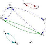
The loop set is formed of the equivalent classes of a based loop of length 5 $\ell_{1}=(8,9,3,4,9)$ and three based loops of length 2, $\ell_{2}=(1,2)$, $\ell_{3}=(8,4)$ and $\ell_{4}=(6,7)$. The partition of $S=\{1,\ldots,9\}$ associated with this loop set is $\pi=(\{1,2\},\{3,4,8,9\},\{5\},\{6,7\})$.

Figure 1: A loop set on the complete graph $K_{9}$

1.2.2 Restriction of the coalescent process to a subset

In our model:

1. each element of $S$ plays the same role,

2. for every subset $A$ of $S$, the Poisson tuple set inside $A$ at time $t$, $\mathcal{P}_{S}(t,A)$ has the same distribution as $\mathcal{P}_{A,p_{S|A}}\Big{(}G_{p}\big{(}\frac{|A|}{|S|}\big{)}t\Big{)}$ where

   $$p_{S|A}(k)=\Big{(}\frac{|A|}{|S|}\Big{)}^{k}\frac{p(k)}{G_{p}\big{(}\frac{|A|}{|S|}\big{)}}\text{ for every }k\in\operatorname{\mathbb{N}}^{*}$$

   and is independent of $\mathcal{P}_{S}(t)\setminus\mathcal{P}_{S}(t,A)$.

We can deduce from these properties a formula for the block size distribution of the coalescent process associated with $\mathcal{P}_{S}(t,A)$ for every subset $A$ of $S$:

Proposition 1.6.

For $x\in S$, let $\Pi_{S,p}^{(x)}(t)$ denote the block of the partition $\Pi_{S,p}(t)$ that contains $x$. Let $A$ be a subset of $S$ that contains $x$. For $k\in\{1,\ldots,|S|\}$,

$$\operatorname{\mathbb{P}}\left(\Big{\lvert}\Pi_{A,p_{S|A}}^{(x)}\Big{(}tG_{p}\big{(}\frac{|A|}{|S|}\big{)}\Big{)}\Big{\rvert}=k\right)=H_{p}(t,|S|,|A|,k)\operatorname{\mathbb{P}}(|\Pi_{S,p}^{(x)}(t))|=k)$$ (1.5)

where

$$H_{p}(t,n,m,k)=\left(\prod_{i=1}^{k-1}\frac{m-i}{n-i}\right)e^{t\big{(}1-G_{p}(1-\frac{k}{n})-G_{p}(\frac{m}{n})+G_{p}(\frac{m-k}{n})\big{)}}$$

with the convention $\prod_{i=1}^{0}=1$.
In particular,

$$\operatorname{\mathbb{E}}\big{(}H_{p}(t,|S|,j,|\Pi_{S,p}^{(x)}(t)|)\big{)}=1\quad\forall j\in\{1,\ldots,|S|\}.$$ (1.6)

Remark 1.7.

The system of equations (1.6) characterizes the distribution of $|\Pi_{S,p}^{(x)}(t))|$ since it can be written as a lower triangular linear system with positive coefficients and with $\operatorname{\mathbb{P}}(|\Pi_{S,p}^{(x)}(t))|=k)$ for $k\in\{1,\ldots,|S|\}$ as unknowns. When $p=\delta_{\{2\}}$, we recover a formula presented by Ràth in a recent preprint (formula (1.1) of [37]): as applications of this formula, Ràth proposes in [37] new proofs of some properties of the component sizes of the Erdös-Rényi random graph in the subcritical and supercritical phases.

Proof of Proposition 1.6.

Let $\Pi^{(x)}_{S,p}(t,A)$ denote the block of $x$ in the partition generated by $\mathcal{P}_{S}(t,A)$. Let $B$ be a subset of $A$ containing $x$:

$$\Pi^{(x)}_{S,p}(t)=B\iff \Pi^{(x)}_{S,p}(t,A)=B\operatorname{and}$$

$$\text{no tuple in}\;\mathcal{P}_{S}(t)\;\text{contains both }\;B\;\text{elements and}\;S\setminus A\;\text{elements}.$$

By property (II),

$$\operatorname{\mathbb{P}}(\Pi^{(x)}_{S,p}(t,A)=B)=\operatorname{\mathbb{P}}\left(\Pi^{(x)}_{A,p_{S|A}}\Big{(}tG_{p}\big{(}\frac{|A|}{|S|}\big{)}\Big{)}=B\right)\operatorname{and}$$

$$\operatorname{\mathbb{P}}(\Pi_{S,p}^{(x)}(t)=B)=\operatorname{\mathbb{P}}(\Pi^{(x)}_{S,p}(t,A)=B)e^{-tI_{S,A}(B)}$$

where

$$I_{S,A}(B) = \mu_{S}(\{\omega\in\mathcal{W}(S),\ \omega\cap B\neq\emptyset\operatorname{and}\omega\cap(S\setminus A)\neq\emptyset\})$$

$$= \mu_{S}(\mathcal{W}(S))-\mu_{S}(\mathcal{W}(S\setminus B))-\mu_{S}(\mathcal{W}(A))+\mu_{S}(\mathcal{W}(A\setminus B))$$

$$= 1-G_{p}\left(1-\frac{|B|}{|S|}\right)-G_{p}\left(\frac{|A|}{|S|}\right)+G_{p}\left(\frac{|A|-|B[}{|S|}\right).$$

Then, formula (1.5) follows from property (I). Indeed,

$$\operatorname{\mathbb{P}}(|\Pi^{(x)}_{S,p}(t,A)|=|B|) = \binom{|A|-1}{|B|-1}\operatorname{\mathbb{P}}(\Pi^{(x)}_{S,p}(t,A)=B)$$

$$= \binom{|A|-1}{|B|-1}\binom{|S|-1}{|B|-1}^{-1}\operatorname{\mathbb{P}}(\Pi_{S,p}^{(x)}(t)=|B|)e^{tI_{S,A}(B)}.$$

Let us note that $H_{p}(t,n,m,k)=0$ if $m$ and $k$ are two integers such that $k\geq m+1$. Therefore, equality (1.5) holds for every $k\in\{1,\ldots,|S|\}$. The sum of over $k\in\{1,\ldots,|S|\}$ of (1.5) yields equation (1.6). ∎

2 Main results

Let us recall that $p$ is a probability distribution on $\operatorname{\mathbb{N}}^{*}$ such that $p(1)<1$. To shorten the notations, we assume now that $S=\llbracket{n}\rrbracket$ and omit the reference to the probability $p$ in the notation: the shorten notations $\mu_{n}$, $\mathcal{P}_{n}$, $\mathcal{P}_{n}(t)$ and $\Pi_{n}(t)$ are used instead of $\mu_{S,p}$, $\mathcal{P}_{S,p}$, $\mathcal{P}_{S,p}(t)$ and $\Pi_{S,p}(t)$. Before stating the main results, let us introduce other notations.

• For $t>0$, $\mathcal{P}^{*}_{n}(t)$ denotes the projection of the set $\mathcal{P}_{n}([0,t]\times\mathcal{W}^{*}(S))$ on $\mathcal{W}^{*}(S)$.

• For $x\in\llbracket{n}\rrbracket$, $\Pi_{n}^{(x)}(t)$ designates the block of the partition $\Pi_{n}(t)$ that contains $x$.

• The $i$-th factorial moment of $p$ is denoted by $m_{p,i}=\sum_{k=i}^{+\infty}k(k-1)\ldots(k-i+1)p(k)$ (let us recall that its probability generating function is denoted by $G_{p}$).

• Let $\tilde{p}$ denote the size-biased probability measure defined on $\operatorname{\mathbb{N}}^{*}$ by $\tilde{p}(k)=\frac{(k+1)p(k+1)}{m^{*}_{p,1}}$ for every $k\in\operatorname{\mathbb{N}}^{*}$, where $m^{*}_{p,1}=m_{p,1}-p(1)$.

• For a positive real $\lambda$ and a probability distribution $\nu$ on $\operatorname{\mathbb{R}}$, let $\text{CPois}(\lambda,\nu)$ denote the compound Poisson distribution with parameters $\lambda$ and $\nu$: $\text{CPois}(\lambda,\nu)$ is the probability distribution of $\sum_{i=1}^{N}X_{i}$, where $N$ is a Poisson distributed random variable with expected value $\lambda$ and $(X_{i})_{i}$ is a sequence of independent random variables with law $\nu$, which is independent of $N$.

• For an integer $u\in\operatorname{\mathbb{N}}^{*}$, a positive real $a$ and a probability measure $\eta$ on $\operatorname{\mathbb{N}}$, we write $\text{BGW}(u,a,\eta)$ for a BGW process with family size distribution $\text{CPois}(a,\eta)$ and $u$ ancestors. Finally for $t>0$ and $u\in\operatorname{\mathbb{N}}^{*}$, we use $T^{(u)}_{p}(t)$ to denote the total number of descendants of a $\text{BGW}(u,tm^{*}_{p,1},\tilde{p})$ process.

2.1 Time to coalescence

The first result shows that the properties of having no singleton and of having only one block have the same sharp threshold function $\frac{n\log(n)}{m^{*}_{p,1}}$.

Theorem 2.1.

Assume that $p$ is a probability distribution on $\operatorname{\mathbb{N}}^{*}$ such that $p(1)<1$, $m_{p,1}$ is finite and $1-G_{p}(1-h)=hm_{p,1}+o(\frac{h}{\log(h)})$ as $h$ tends to $0^{+}$. Let $\tau^{(singl)}_{n}$ and $\tau^{(coal)}_{n}$ denote the first time $t$ for which the partition $\Pi_{n}(t)$ has no singleton and consists of a single block respectively. For every $n\in\operatorname{\mathbb{N}}^{*}$, set $t_{n}=\frac{n}{m^{*}_{p,1}}(\log(n)+a+o(1))$, where $a$ is a fixed real.

1. For every $k\in\operatorname{\mathbb{N}}$, the probability that $\Pi_{n}(t_{n})$ has $k$ singletons converges to $\displaystyle{\frac{e^{-ak}}{k!}}e^{-e^{-a}}$ as $n$ tends to $+\infty$.

2. For every $k\in\operatorname{\mathbb{N}}$, the probability that $\Pi_{n}(t_{n})$ consists of a block of size $n-k$ and $k$ singletons converges to $\displaystyle{\frac{e^{-ak}}{k!}e^{-e^{-a}}}$ as $n$ tends to $+\infty$.

In particular, $\Big{(}m^{*}_{p,1}\dfrac{\tau^{(singl)}_{n}}{n}-\log(n)\Big{)}_{n}$ and $\Big{(}m^{*}_{p,1}\dfrac{\tau^{(coal)}_{n}}{n}-\log(n)\Big{)}_{n}$ converge in distribution to the Gumbel distribution.

Remark 2.2.

• Assumptions on $p$ in Theorem 2.1 are satisfied by probability distributions on $\operatorname{\mathbb{N}}^{*}$ having a finite second moment but not only: the distribution $p$ on $\operatorname{\mathbb{N}}^{*}$ defined by $p(k)=\frac{4}{k(k+1)(k+2)}\;\text{for}\;k\in\operatorname{\mathbb{N}}^{*}$, satisfies the assumptions of Theorem 2.1 and has an infinite variance. Its generating function is

  $$G_{p}(z)=1+2(z-1)+2(z-1)^{2}\frac{1}{z^{2}}(-\log(1-z)-z)\;\forall z\in[0,1].$$

• When $p=\delta_{\{d\}}$ with $d\geq 2$, $\Pi_{n}$ corresponds to the partition made by the components of a random hypergraph process $\mathcal{G}_{n}$ that have similar properties as the $d$-uniform random hypergraph process. It is not surprising to recover the threshold function $\frac{n\log(n)}{d}$ for connectivity of a $d$-uniform random hypergraph (see [35]).

• When $p$ is a logarithmic distribution with parameter $a$ (example 1.5),

  $$m^{*}_{p,1}=\frac{-a^{2}}{(1-a)\log(1-a)}.$$

2.2 Block sizes

Let us turn to the study of the block size of an element at a time proportional to $n$:

Theorem 2.3.

Let $t$ be a positive real. Assume that $p$ has a finite third moment and that $p(1)<1$. Then there exists $C(t)>0$ such that for all $k,n\in\operatorname{\mathbb{N}}^{*}$ and $x\in\llbracket{n}\rrbracket$,

$$|\operatorname{\mathbb{P}}(|\Pi_{n}^{(x)}(nt)|\leq k)-\operatorname{\mathbb{P}}(T^{(1)}_{p}(t)\leq k)|\leq C(t)\frac{k^{2}}{n}.$$

Remark 2.4.

Let us present some properties of the distribution of $T^{(1)}_{p}(t)$ for $t>0$. A BGW process with family size distribution $\text{CPois}(tm^{*}_{p,1},\tilde{p})$ is subcritical if and only if $t<\frac{1}{m_{p,2}}$. Let $q_{p,t}$ denote the extinction probability of such a BGW process starting with one ancestor. It is a decreasing function of $t$.
Moreover,

$$\left\{\begin{array}[]{l}\operatorname{\mathbb{P}}(T^{(u)}_{p}(t)=u)=\displaystyle{e^{-tum^{*}_{p,1}}}\\ \operatorname{\mathbb{P}}(T^{(u)}_{p}(t)=k)=\displaystyle{\frac{u}{k}e^{-ktm^{*}_{p,1}}\sum_{j=1}^{k-u}\frac{(tkm^{*}_{p,1})^{j}}{j!}(\tilde{p})^{\star j}(k-u)}\quad\forall k\geq u+1.\end{array}\right.$$ (2.1)

For $t\leq\frac{1}{m_{p,2}}$, $T^{(u)}_{p}(t)$ is almost surely finite and for $t>\frac{1}{m_{p,2}}$, $\operatorname{\mathbb{P}}(T^{(u)}_{p}(t)<\infty)=(q_{p,t})^{u}<1$.
For $t<\frac{1}{m_{p,2}}$, the distribution of $T^{(u)}_{p}(t)$ has a light tail (that is there exists $s_{0}>0$ such that $\operatorname{\mathbb{E}}(e^{sT^{(u)}_{p}(t)})$ is finite for every $s\leq s_{0}$) if and only if $p$ is a light-tailed distribution (application of Theorem 1 in [19]).

The statement of Theorem 2.3 still holds if $|\Pi_{\llbracket{n}\rrbracket,p}^{(x)}(nt)|$ is replaced by $|\Pi_{\llbracket{n}\rrbracket,p_{n}}^{(x)}(nt_{n})|$ where $(t_{n})_{n}$ and $(p_{n})_{n}$ converge rapidly to $t$ and $p$ respectively:

Corollary 2.5.

Let $(t_{n})_{n}$ be a sequence of positive reals that converges to a real $t$ and let $(p_{n})_{n}$ be a sequence of probability measures on $\operatorname{\mathbb{N}}^{*}$ that converges weakly to a probability measure $p$ on $\operatorname{\mathbb{N}}^{*}$ such that $p(1)<1$. If $\sup_{n\in\operatorname{\mathbb{N}}^{*}}\sum_{k}k^{3}p_{n}(k)$ is finite, $t_{n}m^{*}_{p_{n},1}-tm^{*}_{p,1}=O(\frac{1}{n})$ and $\operatorname{d_{\text{TV}}}(\tilde{p}_{n},\tilde{p})=O(\frac{1}{n})$ then there exists $C(t)>0$ such that $\forall n,k\in\operatorname{\mathbb{N}}^{*}$ and $\forall x\in\llbracket{n}\rrbracket$,

$$|\operatorname{\mathbb{P}}(|\Pi_{\llbracket{n}\rrbracket,p_{n}}^{(x)}(nt_{n})|\leq k)-\operatorname{\mathbb{P}}(T^{(1)}_{p}(t)\leq k)|\leq C(t)\frac{k^{2}}{n}.$$

As a first application of Corollary 2.5, let us consider the block size distribution for the partition defined by the Poisson tuple set inside a macroscopic subset of $\llbracket{n}\rrbracket$ at time $t$:

Corollary 2.6.

Assume that $p$ is a probability distribution on $\operatorname{\mathbb{N}}^{*}$ such that $p(1)<1$. Let $a\in]0,1[$. Set $a_{n}=\lfloor an\rfloor$ and $p_{n}=p_{\llbracket{n}\rrbracket|\llbracket{a_{n}}\rrbracket}$ for $n\in\operatorname{\mathbb{N}}^{*}$. Let $\hat{p}_{a}$ denote the probability distribution on $\operatorname{\mathbb{N}}^{*}$ defined by $\hat{p}_{a}(k)=\frac{a^{k}p(k)}{G_{p}(a)}$ for every $k\in\operatorname{\mathbb{N}}^{*}$.

• There exists $C_{a}(t)>0$ such that for every $k,n\in\operatorname{\mathbb{N}}^{*}$,

  $$\Big{\lvert}\operatorname{\mathbb{P}}\left(|\Pi_{\llbracket a_{n}\rrbracket,p_{n}}^{(1)}\big{(}nG_{p}(\frac{a_{n}}{n})t\big{)}|\leq k\right)-\operatorname{\mathbb{P}}\left(T^{(1)}_{\hat{p}_{a}}\big{(}\frac{G_{p}(a)}{a}t\big{)}\leq k\right)\Big{\rvert}\leq C_{a}(t)\frac{k^{2}}{n}.$$

• For every $u,k\in\operatorname{\mathbb{N}}^{*}$ such that $k\geq u$,

  $$\operatorname{\mathbb{P}}\left(T^{(u)}_{\hat{p}_{a}}\big{(}\frac{G_{p}(a)}{a}t\big{)}=k\right)=a^{k-u}e^{tk(m_{p,1}-G_{p}^{\prime}(a))}\operatorname{\mathbb{P}}(T^{(u)}_{p}(t)=k).$$ (2.2)

Remark 2.7.

1. It is not necessary to assume that the first moments of $p$ are finite since $\hat{p}_{a}$ has finite moments of all order for every $a\in]0,1[$.

2. Formula (2.2) for $u=1$ corresponds to the limit as $n$ tends to $+\infty$ of the identity (1.5) satisfied by $|\Pi_{\llbracket a_{n}\rrbracket,p_{n}}^{(1)}(nG_{p}(\frac{a_{n}}{n})t)|$.

3. If $t\geq 1/m_{p,2}$ and $a$ is equal to the probability extinction $q_{p,t}$ of the BGW$(1,tm^{*}_{p,1},\tilde{p})$ process, then $T^{(1)}_{\hat{p}_{a}}(\frac{G_{p}(a)}{a}t)$ has the same distribution as the total population size of a BGW$(1,tm^{*}_{p,1},\tilde{p})$ process conditioned to become extinct.

Properties (I) and (II) stated in Subsection 1.2.2 and Corollary 2.5 allow to prove a joint limit theorem for the block sizes of two elements:

Corollary 2.8.

Let $x$ and $y$ be two distinct elements of $\llbracket{n}\rrbracket$. For every $t>0$, $j,k\in\operatorname{\mathbb{N}}^{*}$, $\operatorname{\mathbb{P}}(|\Pi_{n}^{(x)}(nt)|=j\operatorname{and}|\Pi_{n}^{(y)}(nt)|=k)$ converges to $\operatorname{\mathbb{P}}(T^{(1)}_{p}(t)=j)\operatorname{\mathbb{P}}(T^{(1)}_{p}(t)=k)$ as $n$ tends to $+\infty$.

2.3 Coagulation equations

Let us consider now the hydrodynamic behavior of the coalescent process $(\Pi_{n}(t))_{t\geq 0}$. A block of size $k$ can be seen as a cluster of $k$ particles of unit mass; at the same time, several clusters of masses $k_{1},\ldots,k_{j}$ can merge into a single cluster of mass ${k_{1}+\ldots+k_{j}}$ at a rate proportional to the product $k_{1}\ldots k_{j}$. The initial state corresponds to the monodisperse configuration ($n$ particles of unit mass). Corollary 2.8 is used to establish the convergence of the average number of blocks of size $k$ at time $nt$ as the number of particles $n$ tends to $+\infty$. The limit seen as a function of $k$ is a solution to coagulation equations:

Theorem 2.9.

Let $p$ be a probability measure on $\operatorname{\mathbb{N}}^{*}$ such that $p(1)<1$ and $m_{p,3}$ is finite.
For $k\in\operatorname{\mathbb{N}}^{*}$, $n\in\operatorname{\mathbb{N}}$ and $t>0$, let $\rho_{n,k}(t)=\frac{1}{nk}\sum_{x=1}^{n}\operatorname{\mathds{1}}_{\{|\Pi_{n}^{(x)}(nt)|=k\}}$ be the average number of blocks of size $k$ and let $\rho_{k}(t)=\frac{1}{k}P(T^{(1)}_{p}(t)=k)$.

1. $(\rho_{n,k}(t))_{n}$ converges to $\rho_{k}(t)$ in $L^{2}$ for every $t>0$.

2. $(\rho_{k}(t),\ k\in\operatorname{\mathbb{N}}^{*}\text{ and }t\geq 0)$ is a solution to the following coagulation equations:

   $$\frac{d}{dt}\rho_{k}(t)=\sum_{j=2}^{+\infty}p(j)\mathcal{K}_{j}(\rho(t),k)$$ (2.3)

   where

   $$\mathcal{K}_{j}(\rho(t),k)=\Big{(}\sum_{\begin{subarray}{c}(i_{1},\ldots,i_{j})\in(\operatorname{\mathbb{N}}^{*})^{j}\\ i_{1}+\cdots+i_{j}=k\end{subarray}}\prod_{u=1}^{j}i_{u}\rho_{i_{u}}(t)\Big{)}\operatorname{\mathds{1}}_{\{j\leq k\}}-jk\rho_{k}(t).$$ (2.4)

Remark 2.10.

1. Consider a medium with integer mass particles and let $\rho_{k}(t)$ denote the density of mass $k$ particles at time $t$. Equation (2.3) describes the evolution of $\rho_{k}(t)$ if for every $j\geq 2$ the number of aggregations of $j$ particles of mass $i_{1},\ldots,i_{j}$ in time interval $[t,t+dt]$ is assumed to be $p(j)\rho_{i_{1}}(t)\ldots\rho_{i_{j}}(t)\kappa_{j}(i_{1},\ldots,i_{j})dt$, where $\kappa_{j}(i_{1},\ldots,i_{j})=i_{1}\cdots i_{j}$ is the multiplicative kernel.
   The first term in $\mathcal{K}_{j}$ describes the formation of a particle of mass $k$ by aggregation of $j$ particles, the second term $jk\rho_{k}(t)$ can be decomposed into the sum of the following two terms:

   • ${\displaystyle jk\rho_{k}(t)\Big{(}\sum_{i=1}^{+\infty}i\rho_{i}(t)\Big{)}^{j-1}}$ that describes the ways a particle of mass $k$ can be aggregated with $j-1$ other particles.

   • ${\displaystyle jk\rho_{k}(t)\sum_{h=1}^{j-1}\binom{j-1}{h}\Big{(}\sum_{i=1}^{+\infty}i(\rho_{i}(0)-\rho_{i}(t))\Big{)}^{h}\Big{(}\sum_{u=1}^{+\infty}u\rho_{u}(t)\Big{)}^{j-1-h}}$. This term is null if the total mass is preserved. Otherwise, the decrease of the total mass can be interpreted as the appearance of a ‘gel’ and this term describes the different ways a particle of mass $k$ can be aggregated with the gel and other particles.

2. The system of equations

   $$\frac{d}{dt}\rho_{k}(t)=\mathcal{K}_{2}(\rho(t),k),\quad\forall k\in\operatorname{\mathbb{N}}^{*}$$

   corresponds to the Flory’s coagulation equations with the multiplicative kernel (see equation (0.1)).
   An application of Theorem 2.9 with $p=\delta_{\{j\}}$ for $j\geq 2$, shows that an approximation of the solution of the system of equations

   $$\frac{d}{dt}\rho_{k}(t)=\mathcal{K}_{j}(\rho(t),k),\quad\forall k\in\operatorname{\mathbb{N}}^{*}$$

   can be constructed by drawing tuples of fixed size $j$.

   Corollary 2.11.

   Let $j$ be an integer greater than or equal to $2$. For $k\in\operatorname{\mathbb{N}}^{*}$, $n\in\operatorname{\mathbb{N}}$ and $t>0$, let $\rho^{(j)}_{n,k}(t)$ be the average number of blocks of size $k$ in the partition $\Pi_{\llbracket{n}\rrbracket,\delta_{\{j\}}}(\frac{nt}{j})$.

   1. $(\rho^{(j)}_{n,k}(t))_{n}$ converges to $\rho^{(j)}_{k}(t)=e^{-tk}\dfrac{(tk)^{\frac{k-1}{j-1}}}{k^{2}(\frac{k-1}{j-1})!}\operatorname{\mathds{1}}_{\{k-1\in(j-1)\operatorname{\mathbb{N}}\}}$ in $L^{2}$ for every $t>0$.

   2. $(\rho^{(j)}_{k}(t),\ k\in\operatorname{\mathbb{N}}^{*}\text{ and }t\geq 0)$ is a solution to the following coagulation equations:

      $$\frac{d}{dt}\rho_{k}(t)=\mathcal{K}_{j}(\rho(t),k)$$ (2.5)

      where $\mathcal{K}_{j}$ is defined by equation (2.4).

3. The function $\rho(t)$ defined by $\rho_{k}(t)=\frac{1}{k}\operatorname{\mathbb{P}}(T^{(1)}_{p}(t)=k)$ for every $k\in\operatorname{\mathbb{N}}^{*}$ gives an explicit solution of (2.3) with mass-conserving property on the interval $[0;\frac{1}{m_{p,2}}]$. Its second moment $\displaystyle{\sum_{k=1}^{+\infty}k^{2}\rho_{k}(t)=(1-tm_{p,2})^{-1}}$ diverges as $t$ tends to $m_{p,2}$.

2.4 Phase transition

As a last application of Theorem 2.3, we show that the block sizes of $(\Pi_{n}(nt))_{t\geq 0}$ undergo a phase transition at $t=\frac{1}{m_{p,2}}$ similar to the phase transition of the Erdös-Rényi random graph process and present some bounds for the sizes of the two largest blocks in the three phases:

Theorem 2.12.

Let $p$ be a probability measure on $\operatorname{\mathbb{N}}^{*}$ such that $p(1)<1$. Let $B_{n,1}(nt)$ and $B_{n,2}(nt)$ denote the first and second largest blocks of $\Pi_{n}(nt)$.

1. Subcritical regime. Let $0<t<\frac{1}{m_{p,2}}$.

   1. Assume that $p$ has a finite moment of order $u$ for some $u\geq 3$. If $(a_{n})_{n}$ is a sequence of reals that tends to $+\infty$, then $\operatorname{\mathbb{P}}(|B_{n,1}(nt)|>a_{n}n^{\frac{1}{u-1}})$ converges to $0$ as $n$ tends to $+\infty$.

   2. Assume that $G_{p}$ is finite on $[0,r]$ for some $r>1$. Let $L_{t}$ denote the moment-generating function of the $\text{CPois}(tm^{*}_{p,1},\tilde{p})$-distribution. Set

      $$h(t)=\sup_{\theta>0}(\theta-\log(L_{t}(\theta))).$$

      Then $h(t)>0$ and for every $a>(h(t))^{-1}$, $\operatorname{\mathbb{P}}(|B_{n,1}(nt)|>a\log(n))$ converges to $0$ as $n$ tends to $+\infty$.

2. Supercritical regime. Assume that $p$ has a finite moment of order three and that $t>\frac{1}{m_{p,2}}$. Let $q_{t}$ denote the extinction probability of a BGW process with one progenitor and $\text{CPois}(tm_{p,1},\tilde{p})$ offspring distribution.
   For every $a\in]1/2,1[$, there exist $b>0$ and $c>0$ such that

   $$\operatorname{\mathbb{P}}\left(\big{\lvert}|B_{n,1}(nt)|-(1-q_{t})n\big{\rvert}\geq n^{a}\right)+\operatorname{\mathbb{P}}\left(|B_{n,2}(nt)|\geq c\log(n)\right)=O(n^{-b}).$$

3. Critical window. Assume that $p$ has a finite moment of order three. For every $\theta\geq 0$, there exists a constant $b>0$ such that for every $c>1$ and $n\in\operatorname{\mathbb{N}}^{*}$

   $$\operatorname{\mathbb{P}}\left(|B_{n,1}(\frac{n}{m_{p,2}}(1+\theta n^{-1/3}))|>cn^{2/3}\right)\leq\frac{c}{b}.$$ (2.6)

Remark 2.13.

Let us provide further information on the subcritical regime (${0<t<\frac{1}{m_{p,2}}}$).

• The upper bound for $|B_{n,1}(nt)|$ given in assertion 1.(b) is reached when ${p=\delta_{2}}$; Indeed, it is known since the Erdös and Rényi’s paper [13] that $\frac{1}{\log(n)}|B_{n,1}(\frac{ns}{2})|$ converges in probability to $(s-1-\log(s))^{-1}$ as $n$ tends to $+\infty$, when $0<s<1$.

• Let us assume now that $p$ is regularly varying with index $-\alpha<-3$: there exists a slowly varying function $\ell$ such that $\sum_{j>k}p(j)=k^{-\alpha}\ell(k)$ $\forall k\in\operatorname{\mathbb{N}}$. Assertion 1.(a) implies that for every $\varepsilon>0$, $\operatorname{\mathbb{P}}(|B_{n,1}(nt)|>n^{\frac{1}{\alpha-1}+\varepsilon})$ tends to $0$ as $n$ tends to $+\infty$. Let us note that $n^{\frac{1}{\alpha-1}}$ corresponds to the order of the largest size for the total progeny of $n$ independent BGW$(1,tm^{*}_{p,1},\tilde{p})$ processes. Indeed, one can show that:

  If $T_{1},\ldots,T_{n}$ are the total progeny of $n$ independent BGW$(1,tm^{*}_{p,1},\tilde{p})$ processes, then for every $1<\alpha_{1}<\alpha<\alpha_{2}$,

  $$\operatorname{\mathbb{P}}(\max_{i=1,\ldots,n}T_{i}>n^{\frac{1}{\alpha_{1}-1}})+\operatorname{\mathbb{P}}(\max_{i=1,\ldots,n}T_{i}<n^{\frac{1}{\alpha_{2}-1}})\underset{n\rightarrow+\infty}{\rightarrow 0}.$$

  An application of the second moment method allows to prove that the largest block size actually grows faster than a positive power of $n$ in the subcritical regime, but gives an exponent smaller than expected:

  Theorem 2.14.

  Assume that $p$ is regularly varying with index $-\alpha<-3$.
  If $t<\frac{1}{m_{p,2}}$ then for every $\alpha^{\prime}>\alpha$, $\operatorname{\mathbb{P}}(\max_{x\in\llbracket{n}\rrbracket}|\Pi_{n}^{(x)}(nt)|\leq n^{\frac{1}{1+\alpha^{\prime}}})$ converges to $0$ as $n$ tends to $+\infty$.

3 The number of singletons and the coalesence time

In a first part, we investigate the distribution of the number of singletons in the partition at time $t$ and the asymptotic distribution of the first time $t$ at which $\Pi_{n}(t)$ does not have singleton. In a second part, we show that the asymptotic distribution of the coalescence time as $n$ tends to $+\infty$ (that is the first time $t$ at which $\Pi_{n}(t)$ consists of a single block) coincides with the asymptotic distribution of the first time $\Pi_{n}$ does not have singleton.

3.1 Number of singletons

Let us observe that the block of an element $x$ in the partition $\Pi_{n}(t)$ is a singleton if and only if tuples in $\mathcal{P}^{*}_{n}(t)$ do not contain $x$. The model is thus a variant of a coupon collector’s problem with group drawings. The exclusion-inclusion lemma provides an exact formula for the number of singletons in $\Pi_{n}(t)$.

Proposition 3.1.

Let $Y_{n,p}(t)$ denote the number of singletons in $\Pi_{n}(t)$. For every ${k\in\{0,\ldots,n\}}$,

$$\operatorname{\mathbb{P}}(Y_{n,p}(t)=k)=\sum_{j=0}^{n-k}(-1)^{j}\frac{n!}{k!j!(n-k-j)!}\exp\Big{(}-t\big{(}1-G_{p}(1-\frac{k+j}{n})-(k+j)G_{p}(\frac{1}{n})\big{)}\Big{)}.$$

Proof.

Let $N_{n}^{(x)}(t)$ denote the number of tuples in $\mathcal{P}^{*}_{n}(t)$ that contain the element $x$.

$$\operatorname{\mathbb{P}}(Y_{n,p}(t)=k)=\sum_{F\subset\llbracket{n}\rrbracket,\ |F|=k}\operatorname{\mathbb{P}}\left(N_{n}^{(x)}(t)>0\;\forall x\not\in F\;\operatorname{and}\;\sum_{x\in F}N_{n}^{(x)}(t)=0\right).$$

By the exclusion-inclusion lemma,

$$\operatorname{\mathbb{P}}\left(N_{n}^{(x)}(t)>0\;\forall x\not\in F\;\operatorname{and}\;\sum_{x\in F}N_{n}^{(x)}(t)=0\right)=\sum_{K\subset\llbracket{n}\rrbracket\setminus F}(-1)^{|K|}\operatorname{\mathbb{P}}\left(\sum_{x\in F\cup K}N_{n}^{(x)}(t)=0\right).$$

We conclude by noting that for any subset $A\subset\llbracket{n}\rrbracket$,

$$\operatorname{\mathbb{P}}\left(\sum_{x\in A}N_{n}^{(x)}(t)=0\right)=\exp\Big{(}-t\mu(w\in\mathcal{W}^{*}(\llbracket{n}\rrbracket),\ w\cap A\neq\emptyset)\Big{)}$$

with

$$\mu\left(w\in\mathcal{W}^{*}(\llbracket{n}\rrbracket),\ w\cap A\neq\emptyset\right)=1-\mu\left(\mathcal{W}(\llbracket{n}\rrbracket\setminus A)\right)-\mu\left(\bigcup_{a\in A}\mathcal{W}(\{a\})\right)\\ =1-G_{p}\left(1-\frac{|A|}{n}\right)-|A|G_{p}\left(\frac{1}{n}\right).$$

∎

An analogy to the classical coupon collector’s problem provides an idea of the average time until $\Pi_{n}$ has no singleton: the number of tuples in $\mathcal{P}^{*}_{n}(t)$ is in average $t\mu_{n}(\mathcal{W}^{*}(\llbracket{n}\rrbracket))$ and the length of nontrivial tuples is in average

$$(\mu_{n}(\mathcal{W}^{*}(\llbracket{n}\rrbracket)))^{-1}\sum_{k=2}^{+\infty}kp(k)(1-\frac{1}{n^{k-1}}).$$

Therefore, the total number of elements drawing before time $t$ and belonging to nontrivial tuples is in average $t(m^{*}_{p,1}+O(\frac{1}{n}))$. If the elements are drawn one by one and not by groups of random sizes, then the solution of the classical coupon collector’s problem, suggests that the time until $\Pi_{n}$ has no singleton would be around $\frac{n\log(n)}{m^{*}_{p,1}}$. The following result shows that this analogy holds in particular when $p$ has a finite second moment.

Theorem (2.1.(i)).

Assume that $m_{p,1}$ is finite and $1-G_{p}(1-h)=hm_{p,1}+o(\frac{h}{\log(h)})$ as $h$ tends to $0^{+}$.

1. For every $a\in\operatorname{\mathbb{R}}$, the number of singletons in $\Pi_{n}$ at time $\frac{n}{m^{*}_{p,1}}(\log(n)+a+o(1))$ converges in distribution to the Poisson distribution with parameter $e^{-a}$ as $n$ tends to $+\infty$.

2. Let $\tau^{(singl)}_{n}$ denote the first time $t$ when $\Pi_{n}(t)$ has no singleton. The sequence

   $$\Big{(}m^{*}_{p,1}\frac{\tau^{(singl)}_{n}}{n}-\log(n)\Big{)}_{n}$$

   converges in distribution to the Gumbel distribution.

Proof.

Set $t_{n}=\frac{n}{m^{*}_{p,1}}(\log(n)+a+o(1))$. Using the notation introduced in proof of Proposition 3.1, the number of singletons in $\Pi_{n}(t_{n})$ is

$$Y_{n,p}(t_{n})=\sum_{x\in\llbracket{n}\rrbracket}\operatorname{\mathds{1}}_{\{N_{x}(t_{n})=0\}}.$$

By the theory of moments, it suffices to show that the factorial moments of any order of $Y_{n,p}(t_{n})$ converge to those of the Poisson distribution with parameter $e^{-a}$ to prove the convergence in distribution.
Let $k\in\operatorname{\mathbb{N}}^{*}$. The $k$-th factorial moment of $Y_{n,p}(t_{n})$ is

$$\operatorname{\mathbb{E}}(Y_{n,p}(t_{n}))_{k}:=\operatorname{\mathbb{E}}(Y_{n,p}(t_{n})(Y_{n,p}(t_{n})-1)\ldots(Y_{n,p}(t_{n})-k+1))\\ =\sum_{F\subset\llbracket{n}\rrbracket,\ |F|=k}k!\operatorname{\mathbb{P}}(\sum_{x\in F}N_{n}^{(x)}(t_{n})=0).$$

Therefore,

$$\operatorname{\mathbb{E}}(Y_{n,p}(t_{n}))_{k}=n^{k}\prod_{i=1}^{k-1}(1-\frac{i}{n})\exp\Big{(}-t_{n}(1-G_{p}(1-\frac{k}{n})-kG_{p}(\frac{1}{n}))\Big{)}.$$

Set $I_{n,k}=-t_{n}\Big{(}1-G_{p}(1-\frac{k}{n})-kG_{p}(\frac{1}{n})\Big{)}+k\log(n)$. It can be rewritten

$$I_{n,k}=-t_{n}\Big{(}1-G_{p}(1-\frac{k}{n})-\frac{k}{n}m_{p,1}-k(G_{p}(\frac{1}{n})-\frac{p(1)}{n})\Big{)}-ak+o(1).$$

Therefore, $I_{n,k}$ converges to $-ak$ as $n$ tends to $+\infty$ since $G_{p}(\frac{1}{n})=\frac{1}{n}p(1)+O(\frac{1}{n^{2}})$ and $1-G_{p}(1-\frac{k}{n})-\frac{k}{n}m_{p,1}=o((n\log(n))^{-1})$ by assumption. This shows that $\operatorname{\mathbb{E}}(Y_{n,p}(t_{n}))_{k}$ converges to $\exp(-ka)$ for every $k\in\operatorname{\mathbb{N}}^{*}$.
To deduce the assertion for $\tau^{(singl)}_{n}$, it suffices to note that for every $x\in\operatorname{\mathbb{R}}$,

$$m^{*}_{p,1}\frac{\tau^{(singl)}_{n}}{n}-\log(n)\leq x\;\iff\;Y_{n,p}(t_{n,x})=0.$$

where $t_{n,x}=\frac{n(\log(n)+x)}{m^{*}_{p,1}}$. ∎

3.2 Time to coalescence

Let $\tau^{(coal)}_{n}$ denote the first time $t$ for which the partition $\Pi_{n}(t)$ consists of a single block.

Theorem (2.1.(ii)).

Assume that $m_{p,1}$ is finite and $1-G_{p}(1-h)=hm_{p,1}+o(\frac{h}{\log(h)})$ as $h$ tends to $0^{+}$. For every $n\in\operatorname{\mathbb{N}}^{*}$, set $t_{n}=\frac{n}{m^{*}_{p,1}}(\log(n)+a+o(1))$ where $a$ is a fixed real.
For every $k\in\operatorname{\mathbb{N}}$, the probability that $\Pi_{n}(t_{n})$ consists of a block of size $n-k$ and $k$ singletons converges to $\displaystyle{\exp(-e^{-a})\frac{e^{-ak}}{k!}}$ as $n$ tends to $+\infty$.
In particular, $\Big{(}m^{*}_{p,1}\dfrac{\tau^{(coal)}_{n}}{n}-\log(n)\Big{)}_{n}$ converges in distribution to the Gumbel distribution.

Proof.

We adapt the proof of Theorem 5.6 given in [26] in the context of Markov loops in the complete graph (that is when $p$ is a logarithmic distribution). For $k\in\operatorname{\mathbb{N}}$, let $H_{n,k}$ denote the event ‘$\Pi_{n}(t_{n})$ consists only of a block of size $n-k$ and $k$ singletons’ and let $J_{n}$ be the event ‘$\Pi_{n}(t_{n})$ has at least two blocks of size greater or equal to $2$’. We have to prove that $\operatorname{\mathbb{P}}(H_{n,k})$ converges to $e^{-e^{-a}}\frac{e^{-ka}}{k!}$. As $\operatorname{\mathbb{P}}(Y_{n,p}=k)$ converges to $e^{-e^{-a}}\frac{e^{-ka}}{k!}$ and is equal to ${\operatorname{\mathbb{P}}(H_{n,k})+\operatorname{\mathbb{P}}(\{Y_{n,p}=k\}\cap J_{n})}$ for $n\geq k+2$, it suffices to prove that $\operatorname{\mathbb{P}}(J_{n})$ converges to $0$. For a subset $F$ of $\llbracket{n}\rrbracket$, let $b_{n}(F)$ denote the probability that $F$ is a block of $\Pi_{n}(t_{n})$ and set $S_{n,r}=\sum_{F\subset\llbracket{n}\rrbracket,|F|=r}b_{n}(F)$ for $r\in\llbracket{n}\rrbracket$. The proof consists in showing that $\sum_{r=2}^{\lfloor n/2\rfloor}S_{n,r}$, which is an upper bound of $\operatorname{\mathbb{P}}(J_{n})$, converges to $0$.
For every subset $A$ of $\llbracket{n}\rrbracket$, let $\mathcal{P}_{n}(t,A)$ denote the set of tuples $w\in\mathcal{P}_{n}(t)$ the elements of which are in $A$. Similarly, let $\mathcal{P}^{*}_{n}(t,A)$ denote the subset of nontrivial tuples of $\mathcal{P}^{*}_{n}(t,A)$. As $\mathcal{P}_{n}(t,F)$ is independent of $\mathcal{P}_{n}(t)\setminus\mathcal{P}_{n}(t,F)$, $b_{n}(F)=b^{(1)}_{n}(F)b^{(2)}_{n}(F)$ where:

• $b^{(1)}_{n}(F)$ is the probability that the partition associated with $\mathcal{P}_{n}(t_{n},F)$ consists of the block $\{F\}$,

• $b^{(2)}_{n}(F)$ is the probability that there is no tuple $w\in\mathcal{P}_{n}(t_{n})$ containing both elements of $F$ and $F^{c}$.

Let $\delta\in]0,1[$. For $|F|\geq n^{1-\delta}$, it is sufficient to replace $b^{(1)}_{n}(F)$ by $1$ as we show that $(b^{(2)}_{n}(F))_{n}$ converges to $0$ rapidly. For $2\leq|F|<n^{1-\delta}$, we use that $b^{(1)}_{n}(F)$ is bounded by the probability that the total number of elements in nontrivial tuples of $\mathcal{P}_{n}(t_{n},F)$ are greater or equal to $|F|$. The value of this upper bound depends only on $|F|$ and $n$. Let denote it $\bar{b}^{(1)}_{n}(|F|)$.

$$S_{n,r}\leq\left\{\begin{array}[]{ll}\sum_{\stackrel{{\scriptstyle F\subset\llbracket{n}\rrbracket}}{{|F|=r}}}b^{(2)}_{n}(F)&\text{if}\;r\geq n^{1-\delta}\\ \bar{b}^{(1)}_{n}(r)\sum_{\stackrel{{\scriptstyle F\subset\llbracket{n}\rrbracket}}{{|F|=r}}}b^{(2)}_{n}(F)&\text{if}\;2\leq r<n^{1-\delta}\end{array}\right.\text{where}\;\bar{b}^{(1)}_{n}(r)=\operatorname{\mathbb{P}}\Big{(}\sum_{w\in\mathcal{P}^{*}_{n}(t_{n},\llbracket{r}\rrbracket)}\ell(w)\geq r\Big{)}.$$

The expression of $b^{(2)}_{n}(F)$ is $\exp\Big{(}-t_{n}(1-G_{p}(\frac{|F|}{n})-G_{p}(1-\frac{|F|}{n}))\Big{)}$. Using that

$$\binom{n}{r}\leq\frac{1}{\sqrt{2\pi r}\sqrt{1-\frac{r}{n}}}(\frac{n}{r})^{r}(1-\frac{r}{n})^{-(n-r)}$$

(see for example [4], formula 1.5 page 4), we obtain:

$$\sum_{F\subset\llbracket{n}\rrbracket,|F|=r}b^{(2)}_{n}(F)\leq\frac{1}{\sqrt{r}}\exp(-nf_{n}(\frac{|F|}{n})),$$

where $f_{n}$ is the function defined by:

$$f_{n}(x)=x\log(x)+(1-x)\log(1-x)+\frac{t_{n}}{n}(1-G_{p}(x)-G_{p}(1-x))\;\text{for}\;x\in]0,1[.$$

To conclude, we need the following two lemmas:

Lemma 3.2.

Let $\delta$ and $\bar{\delta}$ be two positive reals such that $0<\bar{\delta}<\delta<1$. Let $a\in\operatorname{\mathbb{R}}$. Set $t_{n}=\frac{n}{m^{*}_{p,1}}(\log(n)+a+o(1))$ for every $n\in\operatorname{\mathbb{N}}$.
There exists $n_{\delta,\bar{\delta}}>0$ such that for every $n\geq n_{\delta,\bar{\delta}}$, and $F\subset\llbracket{n}\rrbracket$ with $2\leq|F|\leq n^{1-\delta}$,

$$\operatorname{\mathbb{P}}\Big{(}\sum_{w\in\mathcal{P}^{*}_{n}(t_{n},F)}\ell(w)\geq|F|\Big{)}\leq n^{-\frac{\bar{\delta}}{2}|F|}.$$

Lemma 3.3.

Let $f_{n}$ be the function defined by:

$$f_{n}(x)=x\log(x)+(1-x)\log(1-x)+\frac{t_{n}}{n}(1-G_{p}(x)-G_{p}(1-x))\;\forall x\in]0,1[.$$

Let $(u_{n})$ be a positive sequence such that $\liminf_{n}\frac{u_{n}}{\log(n)}>0$. For every $\delta\in]0,1[$, there is an integer $n_{\delta}>0$ such that for $n\geq n_{\delta}$,

• $f_{n}(x)\geq\frac{1-\delta}{2n^{\delta}}\log(n)$ for every $x\in[n^{-\delta},1/2]$,

• $f_{n}(x)+xu_{n}\geq\frac{u_{n}}{n}$ for every $x\in[\frac{2}{n},1/2]$.

Before presenting the proofs of the two lemmas, let us apply them to complete the proof of Theorem 2.1. By Lemma 3.3, for every $0<\bar{\delta}<\delta<1$, there exists $n_{\delta,\bar{\delta}}\in\operatorname{\mathbb{N}}$, such that for every $n>n_{\delta,\bar{\delta}}$,

$$S_{n,r}\leq\left\{\begin{array}[]{ll}\frac{1}{\sqrt{r}}\exp(-nf_{n}(\frac{r}{n}))&\text{ if }r\in[n^{1-\delta},\lfloor n/2\rfloor]\\ \frac{1}{\sqrt{r}}\exp\Big{(}-n\big{(}f_{n}(\frac{r}{n})+\frac{r}{n}\frac{\bar{\delta}}{2}\log(n)\big{)}\Big{)}&\text{ if }r\in[2,n^{1-\delta}].\\ \end{array}\right.$$

We deduce from Lemma 3.3 that for sufficiently large values of $n$,

$$S_{n,r}\leq\left\{\begin{array}[]{ll}\frac{1}{\sqrt{r}}\exp(-\frac{1-\delta}{2}n^{1-\delta}\log(n))&\text{ if }r\in[n^{1-\delta},\lfloor n/2\rfloor]\\ \frac{1}{\sqrt{r}}n^{-\frac{\bar{\delta}}{2}}&\text{ if }r\in[2,n^{1-\delta}].\end{array}\right.$$

Thus for sufficiently large values of $n$, $\operatorname{\mathbb{P}}(J_{n})\leq n^{1-\delta-\frac{\bar{\delta}}{2}}+n\exp(-\frac{1-\delta}{2}n^{1-\delta}\log(n))$. If we take $\delta=\frac{3}{4}$ and $\bar{\delta}=\frac{2}{3}$, we obtain that for sufficiently large values of $n$,

$${\operatorname{\mathbb{P}}(J_{n})\leq n^{-1/12}+ne^{-\frac{1}{8}n^{1/4}\log(n)}}.$$

It remains to prove Lemma 3.2 and Lemma 3.3.

Proof of Lemma 3.2

The random variable $N_{n}(F):=\displaystyle{\sum_{w\in\mathcal{P}^{*}_{n}(t_{n},F)}\ell(w)}$ has a compound Poisson distribution $\text{CPois}(t_{n}\beta_{n,F},\nu_{n,F})$, where

• $\beta_{n,F}=G_{p}(\frac{|F|}{n})-|F|G_{p}(\frac{1}{n})$,

• $\nu_{n,F}(j)=\frac{1}{\beta_{n,F}}\mu(w\in\mathcal{W}^{*}(F),\ \ell(w)=j)=\frac{p(j)}{\beta_{n,F}}\Big{(}(\frac{|F|}{n})^{j}-\frac{|F|}{n^{j}}\Big{)}\;\forall j\in\operatorname{\mathbb{N}}^{*}$.

Its probability generating function at $0\leq s\leq\frac{n}{|F|}$ is:

$$G_{N_{n}(F)}(s)=\exp\Big{(}-t_{n}\beta_{n,F}(1-G_{\nu_{n,F}}(s))\Big{)}\\ =\exp\Big{(}-t_{n}\big{(}G_{p}(\frac{|F|}{n})-G_{p}(s\frac{|F|}{n})-|F|(G_{p}(\frac{1}{n})-G_{p}(\frac{s}{n}))\big{)}\Big{)}.$$

For $2\leq r\leq n$ and $0<\theta\leq\log(\frac{n}{r})$, set

$$\psi_{n,r}(\theta)=\theta r+t_{n}\Big{(}G_{p}(\frac{r}{n})-rG_{p}(\frac{1}{n})-G_{p}(e^{\theta}\frac{r}{n})+rG_{p}(\frac{e^{\theta}}{n})\Big{)}.$$

By Markov’s inequality $\operatorname{\mathbb{P}}(N_{n}(F)\geq|F|)\leq\exp(-\psi_{n,|F|}(\theta))$ for every ${0<\theta\leq\log(\frac{n}{|F|})}$. As $G_{p}^{\prime}$ and $G_{p}^{\prime\prime}$ are increasing functions on $[0,1[$, for $s\in[1,\frac{n}{2r}]$,

$$G_{p}(s\frac{r}{n})-G_{p}(\frac{r}{n})-r(G_{p}(\frac{s}{n})-G_{p}(\frac{1}{n}))\\ \leq\frac{r}{n}(s-1)(G_{p}^{\prime}(s\frac{r}{n})-G_{p}^{\prime}(\frac{1}{n}))\leq\frac{r}{n^{2}}(s-1)(rs-1)G_{p}^{\prime\prime}(1/2).$$

Thus for every $0<\theta\leq\log(\frac{n}{2r})$, $\psi_{n,r}(\theta)\geq rh_{n,r}(\theta)$ with $h_{n,r}(\theta)=\theta-t_{n}\frac{r}{n^{2}}G_{p}^{\prime\prime}(1/2)e^{2\theta}$. The function $h_{n,r}$ has a maximum point at $\theta_{n,r}=\frac{1}{2}\log(\frac{n^{2}}{2t_{n}rG_{p}^{\prime\prime}(1/2)})$, which is less than $\log(\frac{n}{2r})$ for every $r\leq n$ when $n$ is large enough. Its value at $\theta_{n,r}$ is

$$h_{n,r}(\theta_{n,r})=\frac{1}{2}(\log(n)-\log(r)-\log(\frac{t_{n}}{n}))+O(1).$$

Therefore, for every $0<\bar{\delta}<\delta<1$, there exists $n_{\delta,\bar{\delta}}\in\operatorname{\mathbb{N}}$ such that for every $n\geq n_{\delta,\bar{\delta}}\in\operatorname{\mathbb{N}}$ and $2\leq r\leq n^{1-\delta}$, $h_{n,r}(\theta_{n,r})\geq\frac{\bar{\delta}}{2}\log(n)$ and thus $\operatorname{\mathbb{P}}(N_{n}(F)\geq|F|)\leq\exp(-|F|\frac{\bar{\delta}}{2}\log(n))$ for $2\leq|F|\leq n^{1-\delta}$.

Proof of Lemma 3.3

The proof consists in showing that for sufficiently large $n$, $f_{n}$ and $\bar{f}_{n}:x\mapsto f_{n}(x)+xu_{n}$ are increasing functions in $]n^{-\delta},\frac{1}{2}[$ and $]\frac{2}{n},\frac{1}{2}[$ respectively and to compute their values at $n^{-\delta}$ and $\frac{2}{n}$ respectively. Let us prove the result for the function $f_{n}$. By computations, we obtain that for every $x\in]0,1[$,

$$f_{n}^{\prime}(x)=\log(x)-\log(1-x)+\frac{t_{n}}{n}(G_{p}^{\prime}(1-x)-G_{p}(x))\;\operatorname{and}$$

$$f_{n}^{\prime\prime}(x)=\frac{1}{x(1-x)}\Big{(}1-\frac{t_{n}}{n}\sum_{k=2}^{+\infty}k(k-1)g_{k}(x)\Big{)}\;\text{where}\;g_{k}(x)=x(1-x)(x^{k-2}+(1-x)^{k-2}).$$

The first derivative of $g_{k}$ is positive on $]0,\frac{1}{2}[$. As the value of $1-\frac{t_{n}}{n}\sum_{k=2}^{+\infty}k(k-1)g_{k}$ at $0$ is $1$ and at $\frac{1}{2}$ is negative for sufficiently large $n$, we deduce that for sufficiently large $n$, there exists $a_{n}\in]0,\frac{1}{2}[$ such that $f_{n}^{\prime}$ is increasing in $]0,a_{n}[$ and decreasing in $]a_{n},\frac{1}{2}[$. As $f_{n}^{\prime}(\frac{1}{2})=0$ and $f_{n}^{\prime}(n^{-\delta})>0$ for sufficiently large $n$, $f_{n}$ is an increasing function in $]n^{-\delta},\frac{1}{2}[$ for sufficiently large $n$. Finally, using that $1-G_{p}(1-s)-G_{p}(s)=sm^{*}_{p,1}+o(\frac{s}{\log(s)})$ as $s$ tends to $0$, we obtain $f_{n}(\frac{1}{n^{\delta}})=\dfrac{1-\delta}{n^{\delta}}\log(n)+O(n^{-\delta})$. We deduce that for sufficiently large $n$, $f_{n}(x)\geq\dfrac{1-\delta}{2n^{\delta}}\log(n)$ $\forall x\in[\dfrac{1}{n^{\delta}},\frac{1}{2}]$.
As $\bar{f}^{\prime}_{n}=f^{\prime}_{n}+u_{n}$, $f^{\prime}_{n}(\frac{2}{n})=o(1)\log(n)$ and $\bar{f}_{n}(\frac{2}{n})=\frac{2}{n}(O(1)+u_{n})$, we obtain that $\bar{f}_{n}(x)\geq\frac{u_{n}}{n}$ $\forall x\in[\frac{2}{n},\frac{1}{2}]$ for sufficiently large $n$. ∎

4 Block exploration procedure and associated BGW process

In this section, we describe an exploration procedure modeled on the Karp [22] and Martin-Löf [29] exploration algorithm. The aim of this procedure is to find the block of an element $x$ in the partition $\Pi_{n}(t)$ (this block is denoted by $\Pi_{n}^{(x)}(t)$), and to construct a BGW process such that its total population size is an upper bound of $|\Pi_{n}^{(x)}(t)|$.

4.1 Block exploration procedure

For every subset $A$ of $\llbracket{n}\rrbracket$, and $x\in A$, let $\mathcal{P}_{n,x}(t,A)$ denote the set of tuples $w\in\mathcal{P}_{n}(t,A)$ that contain $x$ and let $\mathcal{P}^{*}_{n,x}(t,A)$ denote those that are nontrivial. Let define the set of ‘neighbours’ of $x$ in $A$ as

$$\mathcal{N}_{x}(t,A)=\{y\in A\setminus\{x\},\;\exists w\in\mathcal{P}_{n,x}(t,A)\;\text{that contains}\;y\}.$$

In each step of the algorithm, an element of $\llbracket{n}\rrbracket$ is either active, explored or neutral. Let $A_{k}$ and $H_{k}$ be the sets of active elements and explored vertices in step $k$ respectively in the exploration procedure of the block of $x$.

• In step $0$, $x_{1}=x$ is said to be active ($A_{0}=\{x_{1}\}$) and other elements are neutral.

• In step 1, every neighbour of $x_{1}$ is declared active and $x_{1}$ is said to be an explored element: $A_{1}=\mathcal{N}_{x_{1}}(t,\llbracket{n}\rrbracket)$ and $H_{1}=\{x_{1}\}$.

• In step $k\geq 1$, let us assume that $A_{k-1}$ is not empty. Let $x_{k}$ denote the smallest active element in $A_{k-1}$. Neutral elements that are neighbours of $x_{k}$ are added to $A_{k-1}$ and the status of $x_{k}$ is changed: $A_{k}=A_{k-1}\cup\mathcal{N}_{x_{k}}(t,\llbracket{n}\rrbracket\setminus H_{k-1})\setminus\{x_{k}\}$ and ${H_{k}=H_{k-1}\cup\{x_{k}\}}$. In particular, $|A_{k}|=|A_{k-1}|+\xi_{n,k}(t)-1$ with ${\xi_{n,k}(t)=|\mathcal{N}_{x_{k}}(t,\llbracket{n}\rrbracket\setminus H_{k-1})\setminus A_{k-1}|}$.

The process stops in step $T_{n}(t)=\min(k,\;A_{k}=\emptyset)$. By construction,

$$T_{n}(t)=\min(k,\;\sum_{i=1}^{k}\xi_{n,i}(t)\leq k-1).$$

The block of $x$ is $\Pi_{n}^{(x)}(t)=H_{T_{n}(t)}$ and its size is $T_{n}(t)$.

Example 4.1.

Let $n\geq 10$. Assume that $\mathcal{P}_{n}(t)$ is formed by five tuples $(1,2,3,4)$, $(2,5,2,3)$, $(3,6,4)$, $(6,7)$ and $(8,10)$. The steps of the exploration procedure starting from 1 are

• Step 1: $x_{1}=1$ and $A_{1}=\{2,3,4\}$ so that $\xi_{n,1}(t)=3$.

• Step 2: $x_{2}=2$ and $A_{2}=\{3,4,5\}$ so that $\xi_{n,2}(t)=1$.

• Step 3: $x_{3}=3$ and $A_{3}=\{4,5,6\}$ so that $\xi_{n,3}(t)=1$.

• Step 4: $x_{4}=4$ and $A_{4}=\{5,6\}$ so that $\xi_{n,4}(t)=0$.

• Step 5: $x_{5}=5$ and $A_{5}=\{6\}$ so that $\xi_{n,5}(t)=0$.

• Step 6: $x_{6}=6$ and $A_{6}=\{7\}$ so that $\xi_{n,6}(t)=1$.

• Step 7: $x_{7}=7$ and $A_{7}=\emptyset$ so that $\xi_{n,7}(t)=0$, $T_{n}(t)=7$ and $\Pi^{(1)}_{n}(t)=\{1,2,3,4,5,6,7\}$.

4.2 The BGW process associated with a block

The random variable $\xi_{n,k}(t)$ is bounded above by

$$\zeta^{(1)}_{n,k}(t)=\sum_{w\in\mathcal{P}^{*}_{n,x_{k}}(t,\llbracket{n}\rrbracket\setminus H_{k-1})}\!\!\!(\ell(w)-1)$$

in which a same element is counted as many times as it appears in ${w\in\mathcal{P}^{*}_{n,x_{k}}(t,\llbracket{n}\rrbracket\setminus H_{k-1})}$. To obtain identically distributed random variables in each step, we have to consider also in step $k$, tuples that contain $x_{k}$ and elements of $H_{k-1}$ before time $t$. Let denote this set of tuples $\mathcal{P}_{n,x_{k},H_{k-1}}(t)$ and set $\displaystyle{\zeta^{(2)}_{n,k}(t)=\sum_{w\in\mathcal{P}_{n,x_{k},H_{k-1}}(t)}(\ell(w)-1)}$ and

$$\zeta_{n,k}(t)=\zeta^{(1)}_{n,k}(t)+\zeta^{(2)}_{n,k}(t)=\sum_{w\in\mathcal{P}^{*}_{n,x_{k}}(t,\llbracket{n}\rrbracket)}(\ell(w)-1).$$

The distribution of $\zeta_{n,k}(t)$ is the $\text{CPois}(t\beta_{n},\nu_{n})$-distribution with

$$\beta_{n}=\mu(\{w\in\mathcal{W}^{*}(\llbracket{n}\rrbracket),x\in w\})=\mu(\mathcal{W}^{*}(\llbracket{n}\rrbracket))-\mu(\mathcal{W}^{*}(\llbracket{n}\rrbracket\setminus\{x\}))=1-G_{p}(1-\frac{1}{n})-G_{p}(\frac{1}{n}).$$

and $\forall j\in\operatorname{\mathbb{N}}$,

$$\nu_{n}(j)=\frac{1}{\beta_{n}}\mu(\{w\in\mathcal{W}^{*}(\llbracket{n}\rrbracket),\ x\in w\;\operatorname{and}\;\ell(w)=j+1\})=\frac{p(j+1)}{\beta_{n}}\Big{(}1-(1-\frac{1}{n})^{j+1}-(\frac{1}{n})^{j+1}\Big{)}.$$

Example 4.2.

In example 4.1, the random variables associated with the first three steps of the exploration procedure of the block of 1 are $\zeta^{(1)}_{n,1}(t)=3$, $\zeta^{(2)}_{n,1}(t)=0$, $\zeta^{(1)}_{n,2}(t)=3$, $\zeta^{(2)}_{n,2}(t)=3$, $\zeta^{(1)}_{n,3}(t)=2$ and $\zeta^{(2)}_{n,3}(t)=6$.

Let $\mathcal{F}_{k}=\sigma(H_{j},A_{j},\;j\leq k)$. Let us note that the random variables $\zeta_{n,j}(t)$ and $\zeta_{n,k}(t)$ for $j<k$ are not independent since a same tuple can belong to $\mathcal{P}_{n,x_{k},H_{k-1}}(t)$ and $\mathcal{P}_{n,x_{j},H_{j-1}}(t)$. Nevertheless, since disjoint subsets of tuples in $\mathcal{P}_{n}(t)$ are independent, the random variables $\zeta^{(1)}_{n,j}(t)$ for $j\leq k$ are independent conditionally on $\mathcal{F}_{k-1}$, and the random variable $\zeta^{(1)}_{n,k}(t)$ is independent of $\zeta^{(2)}_{n,k}(t)$ conditionally on $\mathcal{F}_{k-1}$. Therefore, by using independent copies of the Poisson point process $\mathcal{P}_{n}$, we can construct a sequence of nonnegative random variables $(\bar{\zeta}^{(2)}_{n,k}(t))_{k}$ such that:

• $\bar{\zeta}^{(2)}_{n,k}(t)$ has the same distribution as $\zeta^{(2)}_{n,k}(t)$ and is independent of $\zeta^{(1)}_{n,k}(t)$ conditionally on $\mathcal{F}_{k-1}$ for every $k\geq 2$;

• $\bar{\zeta}_{n,k}(t)=\zeta^{(1)}_{n,k}(t)+\bar{\zeta}^{(2)}_{n,k}(t)$ are independent with distribution $\text{CPois}(\beta_{n}t,\nu_{n})$ for every $k\in\operatorname{\mathbb{N}}^{*}$.

Set $\bar{T}_{n}(t)=\min(k,\ \bar{\zeta}_{n,1}(t)+\ldots+\bar{\zeta}_{n,k}(t)=k-1)$. By construction, $\bar{T}_{n}(t)\geq|\Pi_{n}^{(x)}(t)|$. If $\bar{\zeta}_{n,1}(t)$ is seen as the number of offspring of an individual $I$ and $\bar{\zeta}_{n,k}(t)$ for $k\geq 2$ as the number of offspring of the $k$-th individual explored by a breadth-first algorithm of the family tree of $I$, then $\bar{T}_{n}(t)$ is the total number of individuals in the family tree of $I$. We call $(\bar{\zeta}_{n,k}(t))_{k}$ the associated BGW process (a bijection between BGW trees and lattice walks was described by T. E. Harris [18] in Section 6, see also Section 6.2 in [34] for a review).

5 Approximation of block sizes

The number of neighbours of an element is used to approximate the number of active elements added in each step of the exploration process of a block. We begin this section by studying its asymptotic distribution. Next, we prove Theorem 2.3 and Corollary 2.5. Its proof is divided into two steps: we give an upper bound of the deviation between the cumulative distribution function of $|\Pi_{n}^{(x)}(t)|$ and of the total population size of the associated BGW process and then we study the asymptotic distribution of the BGW process associated with $|\Pi_{n}^{(x)}(nt)|$. We end this section by a proof of Corollary 2.8. In this section, the third moment of the distribution $p$ is assumed to be finite.

5.1 Neighbours of an element

Let $V_{n}$ be a subset of $\llbracket{n}\rrbracket$ and let $x\in\llbracket{n}\rrbracket\setminus V_{n}$. The aim of this section is to show that the number of neighbours of $x$ in $\llbracket{n}\rrbracket\setminus V_{n}$ at time $nt$ (denoted by $|\mathcal{N}_{x}(nt,\llbracket{n}\rrbracket\setminus V_{n})|$) converges in law to the $\text{CPois}(tm^{*}_{p,1},\tilde{p})$-distribution if $\frac{V_{n}}{n}$ tends to $0$.
The number of neighbours of $x$ in $\llbracket{n}\rrbracket\setminus V_{n}$ at time $t$ is equal to $\sum_{w\in\mathcal{P}^{*}_{n,x}(t,\llbracket{n}\rrbracket\setminus V_{n})}(\ell(w)-1)$ except if there exists a tuple in $\mathcal{P}^{*}_{n,x}(t,\llbracket{n}\rrbracket\setminus V_{n})$ which has several copies of a same element or if there is an element $y\neq x$ which appears in several tuples of ${\mathcal{P}^{*}_{x}(t,\llbracket{n}\rrbracket\setminus V_{n})}$. The following lemma yields an upper bound for the probability that such an event occurs:

Lemma 5.1.

Let $x\in\llbracket{n}\rrbracket$. Set $F_{n,t}$ be the event ‘some tuples in $\mathcal{P}^{*}_{x}(t,\llbracket{n}\rrbracket)$ contain several copies of a same element or have in common other elements than $x$.’

$$\operatorname{\mathbb{P}}(F_{n,t})\leq\frac{t}{2n^{2}}\left(m_{p,2}+m_{p,3}+\frac{t}{n}(m_{p,2})^{2}\right).$$

Proof.

We study separately the following two events:

• $F^{(1)}_{n,t}$ :‘there exists $y\neq x$ which is in several tuples of $\mathcal{P}^{*}_{n,x}(t)$ or several times in one tuple of $\mathcal{P}^{*}_{n,x}(t)$’

• $F^{(2)}_{n,t}$: ‘some tuples of $\mathcal{P}^{*}_{n,x}(t)$ contain several copies of $x$’.

To compute $\operatorname{\mathbb{P}}(F^{(1)}_{n,t})$, we introduce the random variable $S_{t,x}$ as the total length of tuples in $\mathcal{P}^{*}_{n,x}(t)$ minus the number of copies of $x$ in tuples of $\mathcal{P}^{*}_{n,x}(t)$: $S_{t,x}=\sum_{w\in\mathcal{P}^{*}_{n,x}}\ell_{x}(w)$ where $\ell_{x}(w)$ denotes the number of elements different from $x$ in the tuple $w$. Since elements that form a tuple are chosen independently with the uniform distribution on $\llbracket{n}\rrbracket$,

$$\operatorname{\mathbb{P}}(F^{(1)}_{n,t})=1-\operatorname{\mathbb{E}}\left(\prod_{i=0}^{S_{t,x}-1}(1-\frac{i}{n-1})\right)\leq\frac{1}{2(n-1)}\operatorname{\mathbb{E}}(S_{t,x}(S_{t,x}-1)).$$

By Campbell’s formula, the probability-generating function of $S_{t,x}$ is

$$\operatorname{\mathbb{E}}(u^{S_{t,x}})=\exp\Big{(}\sum_{w\in\mathcal{W}^{*}(\llbracket{n}\rrbracket),\;x\in w}(u^{\ell_{x}(w)}-1)t\mu_{n}(w)\Big{)}.$$

By decomposing $\displaystyle{f_{n}(u)=\sum_{w\in\mathcal{W}^{*}(\llbracket{n}\rrbracket),\;x\in w}(u^{\ell_{x}(w)}-1)\mu_{n}(w)}$ according to the size of a tuple and the number of copies of $x$ in it and then applying the binomial formula, we obtain:

$$f_{n}(u)= \sum_{j=1}^{+\infty}p(j)\sum_{i=1}^{j-1}(u^{j-i}-1)\binom{j}{i}\left(\frac{1}{n}\right)^{i}\left(1-\frac{1}{n}\right)^{j-i}$$

$$= \sum_{j=1}^{+\infty}\frac{p(j)}{n^{j}}\Big{(}(u(n-1)+1)^{j}-u^{j}(n-1)^{j}-n^{j}+(n-1)^{j}\Big{)}$$

$$= G_{p}\left(\frac{1}{n}+u(1-\frac{1}{n})\right)-G_{p}\left(u(1-\frac{1}{n})\right)-1+G_{p}\left(1-\frac{1}{n}\right).$$

We deduce the following formula of $\operatorname{\mathbb{E}}(S_{t,x}(S_{t,x}-1))$ by computing the first two derivatives of $\operatorname{\mathbb{E}}(u^{S_{t,x}})$:

$$\operatorname{\mathbb{E}}(S_{t,x}(S_{t,x}-1))=(1-\frac{1}{n})^{2}\left(t\big{(}G_{p}^{(2)}(1)-G_{p}^{(2)}(1-\frac{1}{n})\big{)}+t^{2}\big{(}G_{p}^{(1)}(1)-G_{p}^{(1)}(1-\frac{1}{n})\big{)}^{2}\right).$$

As the third moment of $p$ is finite,

$$G_{p}^{(1)}(1)-G_{p}^{(1)}(1-\frac{1}{n})\leq\frac{m_{p,2}}{n}\operatorname{and}G_{p}^{(2)}(1)-G_{p}^{(2)}(1-\frac{1}{n})\leq\frac{m_{p,3}}{n}.$$

Thus we obtain:

$$\operatorname{\mathbb{P}}(F^{(1)}_{n,t,k})\leq\frac{t}{2n^{2}}(m_{p,3}+\frac{t}{n}m_{p,2}^{2}).$$

To study $F^{(2)}_{n,t}$, let $N_{x}(w)$ denote the number of copies of $x$ in a tuple $w\in\mathcal{W}^{*}(\llbracket{n}\rrbracket)$:

$$\operatorname{\mathbb{P}}(F^{(2)}_{n,t})=1-\exp\big{(}-t\mu_{n}(w\in\mathcal{W}^{*}(\llbracket{n}\rrbracket),\ N_{x}(w)\geq 2)\big{)}.$$

We have already seen in Proposition 3.1 that

$$\mu_{n}(w\in\mathcal{W}(\llbracket{n}\rrbracket),\ N_{x}(w)\geq 1)=1-G_{p}(1-\frac{1}{n})-G_{p}(\frac{1}{n}).$$

Finally,

$$\mu_{n}(w\in\mathcal{W}^{*}(\llbracket{n}\rrbracket),\ N_{x}(w)=1)=\sum_{k=2}^{+\infty}p(k)\frac{k}{n}(1-\frac{1}{n})^{k-1}=\frac{1}{n}\Big{(}G_{p}^{(1)}(1-\frac{1}{n})-p(1)\Big{)}.$$

Therefore,

$$\mu_{n}(w\in\mathcal{W}^{*}(\llbracket{n}\rrbracket),\ N_{x}(w)\geq 2)=1-G_{p}(1-\frac{1}{n})-\frac{1}{n}G_{p}^{(1)}(1-\frac{1}{n})-G_{p}^{(1)}(\frac{1}{n})+\frac{1}{n}p(1)\leq\frac{1}{2n^{2}}m_{p,2}.$$

In summary, $\operatorname{\mathbb{P}}(F^{(2)}_{n,t})\leq t\mu_{n}(w\in\mathcal{W}^{*}(\llbracket{n}\rrbracket),\ N_{x}(w)\geq 2)\leq\frac{t}{2n^{2}}m_{p,2}.$ ∎

Let us now describe the distribution of the upper bound we have obtained for the number of neighbours of $x$ in $\llbracket{n}\rrbracket\setminus V_{n}$ at time $nt$ and the total variation distance (denoted by $\operatorname{d_{\text{TV}}}$) between it and the compound Poisson distribution $\text{CPois}(tm^{*}_{p,1},\tilde{p})$:

Proposition 5.2.

For a subset $V$ of $\llbracket{n}\rrbracket$ and $x\in\llbracket{n}\rrbracket\setminus V$, set

$$S_{t,V,x}=\sum_{w\in\mathcal{P}^{*}_{x}(t,\llbracket{n}\rrbracket\setminus V)}(\ell(w)-1).$$

• The random variable $S_{nt,V,x}$ has the compound Poisson distribution $\text{CPois}(nt\beta_{V},\nu_{n,V})$ where:

  $$\beta_{n,V}=G_{p}\left(1-\frac{|V|}{n}\right)-G_{p}\left(1-\frac{|V|+1}{n}\right)-G_{p}\left(\frac{1}{n}\right)$$

  $$\nu_{n,V}(j)=\frac{p(j+1)}{\beta_{n,V}}\left(\left(1-\frac{|V|}{n}\right)^{j+1}-\left(1-\frac{|V|+1}{n}\right)^{j+1}-\left(\frac{1}{n}\right)^{j+1}\right)\;\forall j\in\operatorname{\mathbb{N}}.$$

• $\operatorname{d_{\text{TV}}}\left(\text{CPois}(nt\beta_{n,V},\nu_{n,V}),\text{CPois}(tm^{*}_{p,1},\tilde{p})\right)\leq 2tm_{p,2}\left(\frac{|V|}{n}+\frac{1}{2n}\right)+\frac{t}{2n}.$

Proof.

• By definition of the Poisson tuple set, $S_{nt,V,x}$ has the compound Poisson distribution $\text{CPois}(nt\beta_{V},\nu_{n,V})$ where $\beta_{n,V}=\mu_{n}(w\in\mathcal{W}^{*}(\llbracket{n}\rrbracket\setminus V),\ x\in w)$ and for every $j\in\operatorname{\mathbb{N}}^{*}$,

  $$\nu_{n,V}(j)=\frac{1}{\beta_{n,V}}\mu_{n}(w\in\mathcal{W}^{*}(\llbracket{n}\rrbracket\setminus V),\ x\in w\operatorname{and}\ell(w)=j+1).$$

• The total variation distance between two compound Poisson distributions can be bounded as follows using coupling arguments:

  Lemma 5.3.

  Let $p_{1}$ and $p_{2}$ be two probability measures on $\operatorname{\mathbb{N}}$ and let $\lambda_{1}$ and $\lambda_{2}$ be two positive reals such that $\lambda_{1}\leq\lambda_{2}$. Then

  $$\operatorname{d_{\text{TV}}}(\text{CPois}(\lambda_{1},p_{1}),\text{CPois}(\lambda_{2},p_{2}))\leq 1-e^{-(\lambda_{2}-\lambda_{1})}+\lambda_{1}\operatorname{d_{\text{TV}}}(p_{1},p_{2}).$$

  Proof of Lemma 5.3.

  By Strassen’s theorem, there exist two independent sequences $(X_{i})_{i\in\operatorname{\mathbb{N}}^{*}}$ and $(Y_{i})_{i\in\operatorname{\mathbb{N}}^{*}}$ of i.i.d. random variables with distributions $p_{1}$ and $p_{2}$ respectively such that ${\operatorname{d_{\text{TV}}}(p_{1},p_{2})=\operatorname{\mathbb{P}}(X_{i}\neq Y_{i})}$ for every $i\in\operatorname{\mathbb{N}}\*$. Let $Z_{1}$ and $Z_{2}$ be two independent Poisson-distributed random variables with parameters $\lambda_{1}$ and $\lambda_{2}-\lambda_{1}$ respectively, which are independent of the two sequences $(X_{i})_{i}$ and $(Y_{i})_{i}$ (we take $Z_{2}=0$ if $\lambda_{2}=\lambda_{1}$). Set $Z=Z_{1}+Z_{2}$. Then

  $$\operatorname{\mathbb{P}}\left(\sum_{i=1}^{Z_{1}}X_{i}\neq\sum_{i=1}^{Z}Y_{i}\right)\leq\operatorname{\mathbb{P}}(Z_{2}>0)+\operatorname{\mathbb{P}}\left(\sum_{i=1}^{Z_{1}}X_{i}\neq\sum_{i=1}^{Z_{1}}Y_{i}\right)$$

  and

  $$\operatorname{\mathbb{P}}\left(\sum_{i=1}^{Z_{1}}X_{i}\neq\sum_{i=1}^{Z_{1}}Y_{i}\right)\leq\sum_{k=0}^{+\infty}\operatorname{\mathbb{P}}(Z_{1}=k)\sum_{i=1}^{k}\operatorname{\mathbb{P}}(X_{i}\neq Y_{i})=\operatorname{\mathbb{E}}(Z_{1})\operatorname{d_{\text{TV}}}(p_{1},p_{2}).$$

  ∎

  We apply Lemma 5.3 with $\lambda_{1}=tn\beta_{n,V}$, $\lambda_{2}=tm^{*}_{p,1}$, $p_{1}=\nu_{n,V}$ and $p_{2}=\tilde{p}$ and use the following inequalities with $u=\frac{1}{n}$: $\forall j\in\operatorname{\mathbb{N}}^{*}$, $\forall x,u\geq 0$ such that $x+u\leq 1$,

  $$ju-j(j-1)(xu+\frac{u^{2}}{2})\leq(1-x)^{j}-(1-x-u)^{j}\leq ju.$$ (5.1)

  We obtain $0\leq m^{*}_{p,1}-n\beta_{n,V}\leq m_{p,2}\Big{(}\frac{|V|}{n}+\frac{1}{2n}\Big{)}$ and for every $j\in\operatorname{\mathbb{N}}^{*}$,

  $$n\beta_{n,V}|\nu_{n,V}(j)-\tilde{p}(j)|\leq\\ p(j+1)\Big{(}(j+1)(1-\frac{n\beta_{n,V}}{m^{*}_{p,1}})+j(j+1)\big{(}\frac{|V|}{n}+\frac{1}{2n}\big{)}+\frac{1}{n^{j}}\Big{)}.$$ (5.2)

  Therefore

  $$n\beta_{n,V}\operatorname{d_{\text{TV}}}(\nu_{n,V},\tilde{p})\leq\frac{1}{2}m_{p,2}\big{(}\frac{|V|}{n}+\frac{1}{2n}\big{)}+\frac{1}{2}(m_{p,1}-n\beta_{n,V})+\frac{1}{2n}\\ \leq\frac{1}{2n}\big{(}m_{p,2}(2|V|+1)+1\big{)}$$ (5.3)

  and

  $$\operatorname{d_{\text{TV}}}(\text{CPois}(\lambda_{1},p_{1}),\text{CPois}(\lambda_{2},p_{2}))\leq 1-e^{-t(m_{p,1}-n\beta_{n,V})}+tn\beta_{n,V}\operatorname{d_{\text{TV}}}(\nu_{n,V},\tilde{p})$$

  $$\leq 2tm_{p,2}\Big{(}\frac{|V|}{n}+\frac{1}{2n}\Big{)}+\frac{t}{2n}.$$

∎

In summary, Lemma 5.1 and Proposition 5.2 yield the following result for the number of neighbours of an element:

Proposition 5.4.

For every $x\in\llbracket{n}\rrbracket$ and $V\subset\llbracket{n}\rrbracket\setminus\{x\}$, the total variation distance between the distribution of $|\mathcal{N}_{x}(nt,\llbracket{n}\rrbracket\setminus V)|$ and the $\text{CPois}(tm^{*}_{p,1},\tilde{p})$ distribution is smaller than

$$2tm_{p,2}\Big{(}\frac{|V|}{n}+\frac{1}{2n}\Big{)}+\frac{t}{2n}\big{(}1+m_{p,2}+m_{p,3}+t(m_{p,2})^{2}\big{)}.$$

5.2 Comparison between a block size and the associated BGW process

The aim of this section is to prove that small block sizes at time $nt$ are well approximated by $\bar{T}_{n}(nt)$ which has the same distribution as the total population size of a BGW$(1,nt\beta_{n},\nu_{n})$ process (first step of the proof of Theorem 2.3):

Proposition 5.5.

Let $x\in\llbracket{n}\rrbracket$. For every $k,n\in\operatorname{\mathbb{N}}$ and $t\geq 0$,

$$|\operatorname{\mathbb{P}}(|\Pi_{n}^{(x)}(nt)|\leq k)-\operatorname{\mathbb{P}}(\bar{T}_{n}(nt)\leq k)|\leq\frac{kt}{2n}\big{(}m_{p,2}^{2}(k-1+t)+m_{p,2}(k+2)+m_{p,3}\big{)}.$$

Let us recall that the number of new active elements added in the $j$-th step of the exploration procedure at time $t$ is $\xi_{n,j}(t)=|\mathcal{N}_{x_{j}}(t,\llbracket{n}\rrbracket\setminus H_{j-1})\setminus A_{j-1}|$ where $A_{j-1}$ and $H_{j}=\{x_{1},\ldots,x_{j-1}\}$ are respectively the set of active elements and explored elements in step $j-1$. We have already seen one source of difference between $\xi_{n,j}(t)$ and ${\zeta_{n,j}(t)=\sum_{w\in\mathcal{P}^{*}_{n,x_{j}}(t)}(\ell(w)-1)}$. It is described by the event

$F_{n,t,j}$: ‘some tuples in $\mathcal{P}^{*}_{n,x_{j}}(t,\llbracket{n}\rrbracket\setminus H_{j-1})$ contain several copies of a same element or have in common other elements than $x_{j}$’.

By Lemma 5.1, the probability of this event is bounded by: $\frac{t}{2n^{2}}(m_{p,2}+m_{p,3}+\frac{t}{n}m_{p,2}^{2})$.
There are two other sources of difference described by the following events:

• $\{\bar{\zeta}^{(2)}_{n,j}(t)>0$}: ‘there exists a tuple containing $x_{j}$ and already explored elements (that is elements of $H_{j-1}$)’,

• $K_{n,t,j}$: ‘there exists a tuple in $\mathcal{P}_{n,x_{j}}(t,\llbracket{n}\rrbracket\setminus H_{j-1})$ (i.e. containing $x_{j}$ but no element of $H_{j-1}$) which contains active elements (i.e. elements of $A_{j-1}$)’,

The probability of these two events can be bounded by using the following lemma:

Lemma 5.6.

Let $V$ be a subset of $\llbracket{n}\rrbracket$ and let $x\in\llbracket{n}\rrbracket\setminus V$. For every $t>0$,

$$\operatorname{\mathbb{P}}(\exists w\in\mathcal{P}^{*}_{n,x}(t),\ w\cap V\neq\emptyset)\leq 1-\exp(-\frac{t|V|}{n^{2}}m_{p,2})$$

Proof.

Let $K_{x,V}$ be the subset of tuples $w\in\mathcal{W}^{*}(\llbracket{n}\rrbracket)$ which contain $x$ and some elements of $V$.

$$\operatorname{\mathbb{P}}(\exists w\in\mathcal{P}_{n,x}(t),w\cap V\neq\emptyset)=1-\exp(-t\mu(K_{x,V}))$$

and

$$\mu(K_{x,V}) =\mu(\mathcal{P}_{n,x})-\mu(\mathcal{P}_{n,x}(\llbracket{n}\rrbracket\setminus V))$$

$$=1-G_{p}(1-\frac{1}{n})-\big{(}G_{p}(1-\frac{|V|}{n})-G_{p}(1-\frac{|V|+1}{n})\big{)}$$

$$\leq\frac{|V|}{n^{2}}m_{p,2},$$

where the last upper bound is a consequence of the following inequality:

$$1-(1-au)^{j}-(1-bu)^{j}+(1-(a+b)u)^{j}\leq j(j-1)abu^{2}\;\forall j\in\operatorname{\mathbb{N}}^{*},\;\forall a,b\in\operatorname{\mathbb{R}}_{+}\;\operatorname{and}\;\forall u\in[0,\frac{1}{a+b}[.$$

∎

With the help of these estimates, we prove Proposition 5.5.

Proof of Proposition 5.5.

Set $\Delta_{k}=|\operatorname{\mathbb{P}}(|\Pi_{n}^{(x)}(nt)|\leq k)-\operatorname{\mathbb{P}}(\bar{T}_{n}(nt)\leq k)|$.
Since ${|\Pi_{n}^{(x)}(nt)|\leq\bar{T}_{n}(nt)}$, $\Delta_{k}=\operatorname{\mathbb{P}}(|\Pi_{n}^{(x)}(nt)|\leq k\;\text{and}\;\bar{T}^{(n)}_{nt}>k).$ It is bounded above by

$$\operatorname{\mathbb{P}}(|\Pi_{n}^{(x)}(nt)|\leq k\;\text{and}\;\exists j\leq|\Pi_{n}^{(x)}(nt)|,\ \xi_{n,j}(nt)<\bar{\zeta}_{n,j}(nt))\\ \leq\sum_{j=1}^{k}\operatorname{\mathbb{E}}(\operatorname{\mathds{1}}_{\{|\Pi_{n}^{(x)}(nt)|\geq j\}}\operatorname{\mathbb{P}}(\xi_{n,j}(nt)<\bar{\zeta}_{n,j}(nt)|\mathcal{F}_{j-1})).$$

We have seen that

$$\operatorname{\mathbb{P}}(\xi_{n,j}(nt)<\bar{\zeta}_{n,j}(nt)|\mathcal{F}_{j-1})\leq\operatorname{\mathbb{P}}(\zeta^{(2)}_{n,j}(nt)>0|\mathcal{F}_{j-1})+\operatorname{\mathbb{P}}(K_{n,tn,j}|\mathcal{F}_{j-1})+\operatorname{\mathbb{P}}(F_{n,tn,j}|\mathcal{F}_{j-1})$$

with the notations introduced page • ‣ 5.2. By Lemma 5.6

$$\operatorname{\mathbb{P}}(K_{n,tn,j}|\mathcal{F}_{j-1})\leq\frac{t|A_{j-1}|}{n}m_{p,2}\;\text{and}\;\operatorname{\mathbb{P}}(\zeta^{(n,2)}_{nt,j}>0|\mathcal{F}_{j-1})\leq\frac{t(j-1)}{n}m_{p,2}$$

and by Lemma 5.1

$$\operatorname{\mathbb{P}}(F_{n,tn,j}|\mathcal{F}_{j-1})\leq\frac{t}{2n}(m_{p,2}+m_{p,3}+tm_{p,2}^{2}).$$

Therefore,

$$\Delta_{k}\leq\frac{t}{n}m_{p,2}\sum_{j=1}^{k}\operatorname{\mathbb{E}}(|A_{j-1}|\operatorname{\mathds{1}}_{\{|\Pi_{n}^{(x)}(nt)|\geq j\}})\\ +\frac{t}{2n}\sum_{j=1}^{k}\operatorname{\mathbb{P}}(|\Pi_{n}^{(x)}(nt)|\geq j)(m_{p,3}+(2j-1)m_{p,2}+tm_{p,2}^{2}).$$

By construction $|A_{j-1}|-1=\sum_{i=1}^{j-1}(\xi_{n,i}(nt)-1)$. Let us recall that $\xi_{n,i}(nt)$ has nonnegative integer values, it is bounded above by $\bar{\zeta}_{n,i}(nt)$ and the conditional law of $\bar{\zeta}_{n,i}(nt)$ given $\mathcal{F}_{i-1}$ is equal to the law of $\zeta_{n,1}(nt)$. Thus,

$$\operatorname{\mathbb{E}}(\operatorname{\mathds{1}}_{\{|\Pi_{n}^{(x)}(nt)|\geq j\}}(|A_{j-1}|-1))\leq\sum_{i=1}^{j-1}\operatorname{\mathbb{E}}(\operatorname{\mathds{1}}_{\{|\Pi_{n}^{(x)}(nt)|\geq i\}}\operatorname{\mathbb{E}}(\bar{\zeta}_{n,i}(nt)|\mathcal{F}_{i-1}))\leq(j-1)\operatorname{\mathbb{E}}(\zeta_{n,1}(nt)).$$

with $\operatorname{\mathbb{E}}(\zeta_{n,1}(nt))=tn\sum_{j=1}^{+\infty}jp(j+1)\big{(}1-(1-\frac{1}{n})^{j+1}\big{)}\leq tm_{p,2}$. Therefore,

$$\Delta_{k}\leq\frac{t}{n}m_{p,2}^{2}\sum_{j=1}^{k}(j-1)+\frac{t}{2n}\sum_{j=1}^{k}(m_{p,3}+(2j-1)m_{p,2}+tm_{p,2}^{2})\\ =\frac{kt}{2n}(m_{p,2}^{2}(k-1+t)+m_{p,2}(k+2)+m_{p,3}).$$

∎

5.3 The total progeny of the BGW process associated with a block

Recall that the offspring distribution of the BGW process associated with a block at time $nt$ is the $\text{CPois}(tn\beta_{n},\nu_{n})$-distribution with:

$$\beta_{n}=\mu(\{w\in\mathcal{W}^{*}(\llbracket{n}\rrbracket),x\in w\})=1-G_{p}(1-\frac{1}{n})-G_{p}(\frac{1}{n})\;\operatorname{and}$$

$$\nu_{n}(j)=\frac{1}{\beta_{n}}\mu(\{w\in\mathcal{W}^{*}(\llbracket{n}\rrbracket),\ x\in w\;\operatorname{and}\;\ell(w)=j+1\})\\ =\frac{p(j+1)}{\beta_{n}}\Big{(}1-(1-\frac{1}{n})^{j+1}-(\frac{1}{n})^{j+1}\Big{)}\quad\forall j\in\operatorname{\mathbb{N}}^{*}.$$

We have shown (Proposition 5.2) that the $\text{CPois}(tn\beta_{n},\nu_{n})$-distribution is close to the $\text{CPois}(tm^{*}_{p,1},\tilde{p})$-distribution for large $n$. We now consider the distribution of the total number of individuals in a BGW process with one ancestor and offspring distribution $\text{CPois}(tn\beta_{n},\nu_{n})$. Let us state a general result for the comparison of the total number of individuals in two BGW processes:

Lemma 5.7.

Let $\nu_{1}$ and $\nu_{2}$ be two probability distributions on $\operatorname{\mathbb{N}}$. Let $\operatorname{d_{\text{TV}}}$ denote the total variation distance between probability measures. Let $T_{1}$ and $T_{2}$ be the total population sizes of the BGW processes with one ancestor and offspring distributions $\nu_{1}$ and $\nu_{2}$ respectively.
For every $k\in\operatorname{\mathbb{N}}^{*}$, $|\operatorname{\mathbb{P}}(T_{1}\geq k)-\operatorname{\mathbb{P}}(T_{2}\geq k)|\leq\operatorname{d_{\text{TV}}}(\nu_{1},\nu_{2})\sum_{i=1}^{k-1}\operatorname{\mathbb{P}}(T_{2}\geq i)$.

Proof.

We follow the proof of Theorem 3.20 in [42] which states an analogous result between binomial and Poisson BGW processes. The proof is based on the description of the total population size by means of the hitting time of a random walk and coupling arguments. By Strassen’s theorem, there exist two independent sequences $(X_{i})_{i\in\operatorname{\mathbb{N}}^{*}}$ and $(Y_{i})_{i\in\operatorname{\mathbb{N}}^{*}}$ of i.i.d. random variables with distributions $\nu_{1}$ and $\nu_{2}$ respectively such that ${\operatorname{d_{\text{TV}}}(\nu_{1},\nu_{2})=P(X_{i}\neq Y_{i})}$ for every $i\in\operatorname{\mathbb{N}}\*$. Let $\tau_{1}=\min(n,\ X_{1}+\ldots+X_{n}=n-1)$ and $\tau_{2}=\min(n,\ Y_{1}+\ldots+Y_{n}=n-1)$. $\tau_{1}$ and $\tau_{2}$ have the same laws as $T_{1}$ and $T_{2}$ respectively. Let $k\in\operatorname{\mathbb{N}}^{*}$.

$$|\operatorname{\mathbb{P}}(T_{1}\geq k)-\operatorname{\mathbb{P}}(T_{2}\geq k)|\leq\max\big{(}\operatorname{\mathbb{P}}(\tau_{1}\geq k\;\text{and}\;\tau_{2}<k),\operatorname{\mathbb{P}}(\tau_{1}<k\;\text{and}\;\tau_{2}\geq k)\big{)}.$$

First, let us note that

$$\{\tau_{1}\geq k\;\text{and}\;\tau_{2}<k\}\subset\bigcup_{i=1}^{k-1}\{X_{j}=Y_{j}\;\forall j\leq i-1,\;X_{i}\neq Y_{i}\;\text{and}\;\tau_{1}\geq k\}$$

As $\{X_{j}=Y_{j}\;\forall j\leq i-1\;\text{and}\;\tau_{1}\geq k\}\subset\{\tau_{2}\geq i\}$ for $i\leq k-1$ and $\{\tau_{2}\geq i\}$ depends only on $Y_{1},\ldots,Y_{i-1}$, we obtain:

$$\operatorname{\mathbb{P}}(\tau_{1}\geq k\;\text{and}\;\tau_{2}<k)\leq\sum_{i=1}^{k-1}\operatorname{\mathbb{P}}(\tau_{2}\geq i)\operatorname{\mathbb{P}}(X_{i}\neq Y_{i})=\operatorname{d_{\text{TV}}}(\nu_{1},\nu_{2})\sum_{i=1}^{k-1}\operatorname{\mathbb{P}}(\tau_{2}\geq i).$$

The same upper bound holds for $\operatorname{\mathbb{P}}(\tau_{1}<k\;\text{and}\;\tau_{2}\geq k)$ since

$$\{\tau_{1}<k\;\text{and}\;\tau_{2}\geq k)\}\subset\bigcup_{i=1}^{k-1}\{X_{j}=Y_{j}\;\forall j\leq i-1,\;X_{i}\neq Y_{i}\;\text{and}\;\tau_{2}\geq k\}.$$

and $\{\tau_{2}\geq k\}\subset\{\tau_{2}\geq i\}$ for $i\leq k$. ∎

From Lemma 5.7 and Proposition 5.2, we obtain:

Proposition 5.8.

Let $t>0$ and $n\in\operatorname{\mathbb{N}}^{*}$. Let $\bar{T}_{n}(t)$ and $T^{(1)}_{p}(t)$ denote the total number of individuals in a BGW$(1,t\beta_{n},\nu_{n})$ and BGW$(1,tm^{*}_{p,1},\tilde{p})$ processes respectively.

$$|\operatorname{\mathbb{P}}(\bar{T}_{n}(nt)\geq k)-\operatorname{\mathbb{P}}(T^{(1)}_{p}(t)\geq k)|\leq\frac{t}{2n}(2m_{p,2}+1)\sum_{i=1}^{k-1}\operatorname{\mathbb{P}}(T^{(1)}_{p}(t)\geq i)\quad\text{for every}\;k\in\operatorname{\mathbb{N}}^{*}.$$

Proof of Theorem 2.3.

Theorem 2.3 follows from Propositions 5.5 and 5.8:

$$|\operatorname{\mathbb{P}}(|\Pi_{n}^{(x)}(nt)|\leq k)-\operatorname{\mathbb{P}}(T^{(1)}_{p}(t)\leq k)| \leq |\operatorname{\mathbb{P}}(|\Pi_{n}^{(x)}(nt)|\leq k)-\operatorname{\mathbb{P}}(\bar{T}_{n}(nt)\leq k)|$$

$$+|\operatorname{\mathbb{P}}(\bar{T}_{n}(nt)\leq k)-\operatorname{\mathbb{P}}(T^{(1)}_{p}(t)\leq k)|$$

$$\leq \frac{kt}{2n}\big{(}m_{p,2}^{2}(k-1+t)+m_{p,2}(k+4)+m_{p,3}+1\big{)}.$$

∎

Proof of Corollary 2.5.

To deduce Corollary 2.5, we apply the above inequality to $|\operatorname{\mathbb{P}}(|\Pi_{\llbracket{n}\rrbracket,p_{n}}^{(x)}(nt_{n})|\leq k)-\operatorname{\mathbb{P}}(T^{(1)}_{p_{n}}(t_{n})\leq k)|$. By Lemma 5.7 and Lemma 5.3:

$$|\operatorname{\mathbb{P}}(T^{(1)}_{p_{n}}(t_{n})\leq k)-\operatorname{\mathbb{P}}(T^{(1)}_{p}(t)\leq k)|\leq k\Big{(}|t_{n}m^{*}_{p_{n},1}-tm^{*}_{p,1}|+\max(t_{n}m^{*}_{p_{n},1},tm^{*}_{p,1})\operatorname{d_{\text{TV}}}(\tilde{p}_{n},\tilde{p})\Big{)}.$$

Under the hypotheses of Corollary 2.5, $(m_{p_{n},i})_{n}$ for $i\in\{1,2,3\}$ are bounded, ${|t_{n}m^{*}_{p_{n},1}-tm^{*}_{p,1}|=O(\frac{1}{n})}$ and $\operatorname{d_{\text{TV}}}(\tilde{p}_{n},\tilde{p})=O(\frac{1}{n})$. Therefore, there exists $C(t)>0$ such that for every $k\in\operatorname{\mathbb{N}}^{*}$,

$$|\operatorname{\mathbb{P}}(|\Pi_{n}^{(x)}(nt_{n})|\leq k)-\operatorname{\mathbb{P}}(T^{(1)}_{p}(t)\leq k)|\leq\frac{C(t)k^{2}}{n}.$$

∎

Proof of Corollary 2.6.

Let us now consider $\Pi_{\llbracket a_{n}\rrbracket,p_{n}}^{(1)}(ntG_{p}(\frac{a_{n}}{n}))$, where $a_{n}=\lfloor an\rfloor$ and $p_{n}$ is the probability distribution on $\operatorname{\mathbb{N}}^{*}$ defined by:

$$p_{n}(k)=\left(\frac{a_{n}}{n}\right)^{k}p(k)\frac{1}{G_{p}(\frac{a_{n}}{n})}\;\forall k\in\operatorname{\mathbb{N}}^{*}.$$

Set $t_{n}=t\frac{n}{a_{n}}G_{p}(\frac{a_{n}}{n})$ for $n\in\operatorname{\mathbb{N}}^{*}$. To prove that there exists $C_{a}(t)>0$ such that for every $k,n\in\operatorname{\mathbb{N}}^{*}$,

$$\left|\operatorname{\mathbb{P}}\left(|\Pi_{\llbracket a_{n}\rrbracket,p_{n}}^{(1)}(ntG_{p}(\frac{a_{n}}{n}))|\leq k\right)-\operatorname{\mathbb{P}}\left(T^{(1)}_{\hat{p}_{a}}(t\frac{G_{p}(a)}{a}))\leq k\right)\right|\leq C_{a}(t)\frac{k^{2}}{n},$$

it suffices to verify that Corollary 2.5 applies to the sequences $(t_{n})_{n}$ and $(p_{n})_{n}$:

1. Since $|\frac{a_{n}}{n}-a|\leq\frac{1}{n}$ and $G_{p}^{\prime}$ is bounded on $[0,a]$, $t_{n}-t\frac{G_{p}(a)}{a}=O(\frac{1}{n})$.

2. The third moment of $p_{n}$ is bounded since $\sum_{k=1}^{+\infty}k^{3}p_{n}(k)\leq\frac{1}{G_{p}(a_{n})}\sum_{k=1}^{+\infty}k^{3}a^{k}p(k)$ for every $n\in\operatorname{\mathbb{N}}^{*}$.

3. The difference $\Delta_{n}:=t_{n}m_{p_{n},1}^{*}-t\frac{G_{p}(a)}{a}m_{\hat{p}_{a},1}^{*}$ can be split into the sum of two terms:

   $$\Delta_{n,1} = t\left(\frac{n}{a_{n}}-\frac{1}{n}\right)\sum_{k\geq 2}k(\frac{a_{n}}{n})^{k}p(k)=O(\frac{1}{n}),$$

   $$\Delta_{n,2} = \frac{1}{a}\sum_{k\geq 2}((\frac{a_{n}}{n})^{k}-a^{k})kp(k).$$

   By applying the following inequality

   $$|x^{k}-y^{k}|\leq k|x-y|\max(|x|,|y|)^{k-1}\;\forall x,y\in\operatorname{\mathbb{R}},$$ (5.4)

   we obtain $|\Delta_{n,2}|\leq\frac{1}{an}\sum_{k\geq 2}k^{2}a^{k-1}p(k)=O(\frac{1}{n})$.

4. The last assumption of Corollary 2.5 concerns the total variation distance between the probability distributions $\tilde{p}_{n}$ and $\widetilde{(\hat{p}_{a})}$ defined by:

   $$\tilde{p}_{n}(k)=\frac{1}{S(\frac{a_{n}}{n})}(k+1)(\frac{a_{n}}{n})^{k}p(k+1)\operatorname{and}\widetilde{(\hat{p}_{a})}(k)=\frac{1}{S(a)}(k+1)a^{k}p(k+1)\;\forall k\in\operatorname{\mathbb{N}}^{*},$$

   where $S(x)=\sum_{j\geq 2}jx^{j}p(j)$ for $x\in[0,1[$.
   Let us note that $d_{\operatorname{d_{\text{TV}}}}(\tilde{p}_{n},\widetilde{(\hat{p}_{a})})\leq\frac{1}{S(a)}\sum_{k\geq 2}kp(k)|(\frac{a_{n}}{n})^{k}-a^{k}|$. Therefore, by inequality (5.4), $\operatorname{d_{\text{TV}}}(\tilde{p}_{n},\widetilde{(\hat{p}_{a})})=O(\frac{1}{n})$.

In conclusion, the four assumptions of Corollary 2.5 are satisfied.

Relation (2.2) between the probability mass functions of $T^{(u)}_{\hat{p}_{a}}(\frac{G_{p}(a)}{a}t)$ and $T^{(u)}_{p}(t)$ can be easily proven by applying formula (2.1) for the probability mass function of $T^{(u)}_{p}(t)$ (see Appendix A.2 for a proof of (2.1)) and by expressing the probability mass function of $\text{CPois}(\lambda G_{\tilde{p}}(a),\widehat{(\tilde{p})}_{a})$ in terms of the probability mass function of $\text{CPois}(\lambda,\tilde{p})$ (see Lemma A.5). ∎

5.4 Asymptotic distribution of two block sizes

Let us prove Corollary 2.8 stating that under the assumptions of Theorem 2.3, the block sizes of two elements converge in law to the total population sizes of two independent BGW$(1,tm^{*}_{p,1},\tilde{p})$ processes.

Proof of Corollary 2.8.

The proof is similar to the proof presented in [3] in order to study the joint limit of the component sizes of two vertices in the Erdös-Rényi random graph process. It is based on the properties (I) and (II) stated in Subsection 1.2.2.
Let $x$ and $y$ be two distinct vertices and let $j,k$ be two nonnegative integers. We have to study the convergence of $\operatorname{\mathbb{P}}(|\Pi_{n}^{(x)}(nt)|=j\operatorname{and}|\Pi_{n}^{(y)}(nt)|=k)$. First, let us note that by (I), for every $n\geq j$, $\operatorname{\mathbb{P}}(y\in\Pi_{n}^{(x)}(nt)\mid|\Pi_{n}^{(x)}(nt)|=j)=\frac{j-1}{n-1}$. Therefore, ${\operatorname{\mathbb{P}}(y\in\Pi_{n}^{(x)}(nt)\operatorname{and}|\Pi_{n}^{(x)}(nt)|=j)}$ converges to $0$ as $n$ tends to $+\infty$.
It remains to study $\operatorname{\mathbb{P}}(y\not\in\Pi_{n}^{(x)}(nt)\operatorname{and}|\Pi_{n}^{(x)}(nt)|=j\operatorname{and}|\Pi_{n}^{(y)}(nt)|=k)$ which can be written:

$$\operatorname{\mathbb{P}}(|\Pi_{n}^{(y)}(nt)|=k\mid y\not\in\Pi_{n}^{(x)}(nt)\operatorname{and}|\Pi_{n}^{(x)}(nt)|=j)\operatorname{\mathbb{P}}(y\not\in\Pi_{n}^{(x)}(nt)\operatorname{and}|\Pi_{n}^{(x)}(nt)|=j).$$

Since $\operatorname{\mathbb{P}}(y\not\in\Pi_{n}^{(x)}(nt)\operatorname{and}|\Pi_{n}^{(x)}(nt)|=j)=(1-\frac{j-1}{n-1})\operatorname{\mathbb{P}}(|\Pi_{n}^{(x)}(nt)|=j)$, it converges to $\operatorname{\mathbb{P}}(T^{(1)}_{p}(t)=j)$ by Theorem 2.3.
By (II),

$$\operatorname{\mathbb{P}}(|\Pi_{n}^{(y)}(nt)|=k\mid y\not\in\Pi_{n}^{(x)}(nt)\operatorname{and}|\Pi_{n}^{(x)}(nt)|=j)=\operatorname{\mathbb{P}}(|\Pi_{\llbracket{n-j}\rrbracket,p_{n,j}}^{(y)}((n-j)t_{n,j})|=k)$$

where $t_{n,j}=\frac{tn}{n-j}G_{p}(1-\frac{j}{n})$ and $p_{n,j}=p_{\llbracket{n}\rrbracket|\llbracket{n-j}\rrbracket}$ (i.e. $p_{n,j}(k)=(1-\frac{j}{n})^{k}\frac{p(k)}{G_{p}(1-\frac{j}{n})}$ for every $k\in\operatorname{\mathbb{N}}^{*}$).

Let us verify that Corollary 2.5 can be applied to the sequences $(t_{n,j})_{n}$ and $(p_{n,j})_{n}$.

• First, $(t_{n,j})_{n}$ converges to $t$, $(p_{n,j})_{n}$ converges weakly to $p$, and $(m_{p_{n,j},3})_{n}$ converges to $m_{p,3}$.

• By inequality (5.1), $0\leq tm^{*}_{p,1}-t_{n,j}m^{*}_{p_{n,j},1}\leq\frac{tj}{n}m_{p,2}$.

• Finally, let us show that $\operatorname{d_{\text{TV}}}(\tilde{p}_{n,j},\tilde{p})=O(\frac{1}{n})$. For $k\in\operatorname{\mathbb{N}}$,

  $$\tilde{p}(k)-\tilde{p}_{n,j}(k)=(k+1)p(k+1)\frac{V_{n}(k)}{m_{p,1}S_{n}}$$

  with

  $$V_{n}(k)=\sum_{\ell\geq 1}(\ell+1)p(\ell+1)\Big{(}(1-\frac{j}{n})^{\ell+1}-(1-\frac{j}{n})^{k+1}\Big{)}\;\text{and}\;S_{n}=\sum_{\ell\geq 1}(\ell+1)p(\ell+1)(1-\frac{j}{n})^{\ell+1}.$$

  Using that the first $k$ terms in $V_{n}(k)$ are positive and the others are nonpositive, we obtain $|V_{n}(k)|\leq\frac{j}{n}\max(km^{*}_{p,1},m_{p,2})$ for every $k\in\operatorname{\mathbb{N}}$.
  As $(1-x)^{\ell}\geq 1-\ell x$ for every $x\geq 0$ and $\ell\in\operatorname{\mathbb{N}}^{*}$, $S_{n}\geq m^{*}_{p,1}-\frac{j}{n}(m^{*}_{p,1}+m_{p,2})$. Therefore, $\operatorname{d_{\text{TV}}}(\tilde{p}_{n,j},\tilde{p})\leq\frac{j}{n}m_{p,2}\big{(}m^{*}_{p,1}-\frac{j}{n}(m^{*}_{p,1}+m_{p,2})\big{)}^{-1}=O(\frac{1}{n})$.

Consequently, $\operatorname{\mathbb{P}}(|\Pi_{n}^{(y)}(nt)|=k\mid y\not\in\Pi_{n}^{(x)}(nt)\operatorname{and}|\Pi_{n}^{(x)}(nt)|=j)$ converges to $\operatorname{\mathbb{P}}(T^{(1)}_{p}=k)$, which completes the proof. ∎

6 Hydrodynamic behavior of the coalescent process

This section is devoted to the proof of Theorem 2.9 describing the asymptotic limit of the average number of blocks having the same size.

1. Let $t>0$ and $k\in\operatorname{\mathbb{N}}^{*}$. First, we prove that $\rho_{n,k}(t)=\frac{1}{nk}\sum_{x=1}^{n}\operatorname{\mathds{1}}_{\{|\Pi_{n}^{(x)}(nt)|=k\}}$ converges in $L^{2}$ to $\rho_{k}(t)=\frac{1}{k}\operatorname{\mathbb{P}}(T^{(1)}_{p}(t)=k)$. Theorem 2.3 and Corollary 2.8 imply the convergence of the first two moments of $\rho_{n,k}(t)$ to $\rho_{k}(t)$ and $(\rho_{k}(t))^{2}$ respectively and thus the $L^{2}$ convergence of $(\rho_{n,k}(t))_{n}$. Indeed, $\operatorname{\mathbb{E}}(\rho_{n,k}(t))=\frac{1}{k}\operatorname{\mathbb{P}}(|\Pi_{n}^{(1)}(nt)|=k)$ converges to $\rho_{k}(t)$. The second moment is

   $$\operatorname{\mathbb{E}}((\rho_{n,k}(t))^{2})=\frac{1}{nk^{2}}\operatorname{\mathbb{P}}(|\Pi_{n}^{(1)}(nt)|=k)+(1-\frac{1}{n})\frac{1}{k^{2}}\operatorname{\mathbb{P}}(|\Pi_{n}^{(1)}(nt)|=k\;\operatorname{and}\;|\Pi_{n}^{(2)}(nt)|=k).$$

   The first term converges to 0 and the second term converges to $(\rho_{k}(t))^{2}$.

2. It remains to show that $\{\rho(t),\;t\in\operatorname{\mathbb{R}}_{+}\}$ is solution of the coagulation equations (2.3):

   $$\frac{d}{dt}\rho_{k}(t)=\sum_{j=2}^{+\infty}p(j)\mathcal{K}_{j}(\rho(t),k)$$

   where

   $$\mathcal{K}_{j}(\rho(t),k)=\Big{(}\sum_{\begin{subarray}{c}(i_{1},\ldots,i_{j})\in(\operatorname{\mathbb{N}}^{*})^{j}\\ i_{1}+\cdots+i_{j}=k\end{subarray}}\prod_{u=1}^{j}i_{u}\rho_{i_{u}}(t)\Big{)}\operatorname{\mathds{1}}_{\{j\leq k\}}-kj\rho_{k}(t).$$

   By definition of $\rho(t)$, for $j\in\operatorname{\mathbb{N}}\setminus\{0,1\}$,

   $$\mathcal{K}_{j}(\rho(t),k)=\operatorname{\mathbb{P}}(T^{(j)}_{p}(t)=k)\operatorname{\mathds{1}}_{\{j\leq k\}}-j\operatorname{\mathbb{P}}(T^{(1)}_{p}(t)=k),$$

   where $T^{(\ell)}_{p}(t)$ denotes the total progeny of a BGW$(\ell,tm^{*}_{p,1},\tilde{p})$ process for every $\ell\in\operatorname{\mathbb{N}}^{*}$.
   The probability distribution of $T^{(\ell)}_{p}(t)$ is computed in the appendix (Lemma A.2):

   $$\left\{\begin{array}[]{l}\operatorname{\mathbb{P}}(T^{(\ell)}_{p}(t)=\ell)=\displaystyle{e^{-t\ell m^{*}_{p,1}}}\\ \operatorname{\mathbb{P}}(T^{(\ell)}_{p}(t)=k)=\displaystyle{\frac{\ell}{k}e^{-ktm^{*}_{p,1}}\sum_{h=1}^{k-\ell}\frac{(tm^{*}_{p,1}k)^{h}}{h!}(\tilde{p})^{\star h}(k-\ell)}\quad\forall k\geq\ell+1.\end{array}\right.$$

   For $k=1$, $\rho_{1}$ is solution of the equation $\frac{d}{dt}\rho_{1}(t)=-m^{*}_{p,1}\rho_{1}(t)$ and the right hand side term is equal to $\sum_{j=2}^{+\infty}p(j)\mathcal{K}_{j}(\rho(t),1)$.
   Let us assume now that $k\geq 2$.

   $$\sum_{j=2}^{+\infty}p(j)\mathcal{K}_{j}(\rho(t),k)=\frac{e^{-tkm^{*}_{p,1}}}{k}\left(kp(k)+\sum_{j=2}^{k-1}\sum_{h=1}^{k-j}\frac{(tm^{*}_{p,1}k)^{h}}{h!}jp(j)(\tilde{p})^{\star h}(k-j)\right)\\ -m^{*}_{p,1}\operatorname{\mathbb{P}}(T^{(1)}_{p}(t)=k).$$

   By using that $jp(j)=m^{*}_{p,1}\tilde{p}(j-1)$ for every $j\geq 2$ and by inverting the two sums we obtain

   $$\sum_{j=2}^{+\infty}p(j)\mathcal{K}_{j}(\rho(t),k)=\frac{m^{*}_{p,1}}{k}e^{-tkm^{*}_{p,1}}\sum_{h=1}^{k-1}\frac{(tm^{*}_{p,1}k)^{h-1}}{(h-1)!}(\tilde{p})^{\star h}(k-1)-m^{*}_{p,1}\operatorname{\mathbb{P}}(T^{(1)}_{p}(t)=k).$$

   Since the right-hand side of the last formula is equal to $\frac{1}{k}\frac{d}{dt}\operatorname{\mathbb{P}}(T^{(1)}_{p}(t)=k)$,

   $$\frac{d}{dt}\rho_{k}(t)=\sum_{j=2}^{+\infty}p(j)\mathcal{K}_{j}(\rho(t),k)$$

   This completes the proof of Theorem 2.9.

7 Phase transition

The expectation of the compound Poisson distribution $\text{CPois}(tm^{*}_{p,1},\tilde{p})$ is $tm_{p,2}$. Thus the limiting BGW process associated with a block is subcritical, critical or supercritical depending on whether $t$ is smaller, equal or larger than $\frac{1}{m_{p,2}}$. This section is devoted to the proofs of Theorems 2.12 and 2.14, which provide some results on the size of the largest block at time $nt$ in these three cases.

7.1 The subcritical regime

Let us assume that $t<\frac{1}{m_{p,2}}$. An application of the block exploration procedure and Fuk-Nagaev inequality allows to prove that, if the moment of $p$ of order $u$ is finite for some $u\geq 3$, then the largest block size at time $nt$ is not greater than $n^{1/(u-1)+\varepsilon}$ for any $\varepsilon>0$ with probability that converges to $1$. If the probability generating function of $p$ is assumed to be finite for some real greater than 1, then it can be shown using a Chernoff bound that the largest block size at time $nt$ is at most of order $\log(n)$ with probability that converges to $1$.

Theorem (2.12.(1)).

Let $0<t<\frac{1}{m_{p,2}}$.

1. Assume that $p$ has a finite moment of order $u$ for some $u\geq 3$. If $(a_{n})_{n}$ is a sequence of reals that tends to $+\infty$, then $\operatorname{\mathbb{P}}(\max_{x\in\llbracket{n}\rrbracket}|\Pi_{n}^{(x)}(nt)|>a_{n}n^{\frac{1}{u-1}})$ converges to $0$ as $n$ tends to $+\infty$.

2. Assume that $G_{p}$ is finite on $[0,r]$ for some $r>1$. Set $h(t)=\sup_{\theta>0}(\theta-\log(L_{t}(\theta)))$ where $L_{t}$ is the moment-generating function of the compound Poisson distribution $\text{CPois}(tm^{*}_{p,1},\tilde{p})$.
   Then $h(t)>0$ and for every $a\geq(h(t))^{-1}$, $\operatorname{\mathbb{P}}(\max_{x\in\llbracket{n}\rrbracket}|\Pi_{n}^{(x)}(nt)|>a\log(n))$ converges to $0$ as $n$ tends to $+\infty$.

Proof.

For $k\in\operatorname{\mathbb{N}}^{*}$, let $Z_{k}(t)$ denote the number of blocks of size greater than $k$ at time $t$. Since each element of $\llbracket{n}\rrbracket$ plays the same role,

$$\operatorname{\mathbb{P}}(\max_{x\in\llbracket{n}\rrbracket}|\Pi_{n}^{(x)}(t)|>k)\leq\operatorname{\mathbb{P}}(Z_{k}(t)>k)\leq\frac{\operatorname{\mathbb{E}}(Z_{k}(t))}{k}=\frac{n}{k}\operatorname{\mathbb{P}}(|\Pi_{n}^{(1)}(t)|>k).$$ (7.1)

By construction of the random variables $\xi_{n,j}(t)$ and $\bar{\zeta}_{n,j}(t)$,

$$\operatorname{\mathbb{P}}(|\Pi_{n}^{(1)}(t)|>k)\leq\operatorname{\mathbb{P}}(\sum_{i=1}^{k}\xi_{n,i}(t)\geq k)\leq\operatorname{\mathbb{P}}(\sum_{i=1}^{k}\bar{\zeta}_{n,i}(t)\geq k).$$

1. First, let us assume that $p$ has a finite moment of order $u\geq 3$. Set $e_{n}(t)=\operatorname{\mathbb{E}}(\bar{\zeta}_{n,1}(t))$ and $X_{i,n}=\bar{\zeta}_{n,i}(nt)-e_{n}(nt)$ for $i\in\llbracket{n}\rrbracket$.
   Let us recall the Fuk-Nagaev inegality, we shall apply to the sequence $(X_{i,n})_{i=1\ldots,k}$:

   Theorem (Corollary 1.8 of [31]).

   Let $s\geq 2$ and let $Y_{1},\ldots,Y_{k}$ be independent random variables such that $\operatorname{\mathbb{E}}(\max(Y_{i},0)^{s})<+\infty$ and $\operatorname{\mathbb{E}}(Y_{i})=0$ for every ${i\in\{1,\ldots,k\}}$. Set $A_{s,k}^{+}=\sum_{i=1}^{k}\operatorname{\mathbb{E}}(\max(Y_{i},0)^{s})$ and $B_{k}=\sum_{i=1}^{k}\operatorname{Var}(Y_{i})$.
   For every $x>0$,

   $$P(\sum_{i=1}^{k}Y_{i}\geq x)\leq x^{-s}c^{(1)}_{s}\sum_{i=1}^{k}\operatorname{\mathbb{E}}(\max(Y_{i},0)^{s})+\exp(-c^{(2)}_{s}\frac{x^{2}}{B_{k}}),$$

   where $c^{(1)}_{s}=(1+2/s)^{s}$ and $c^{(2)}_{s}=2(s+2)^{-2}e^{-s}$.

   We begin by proving that $\operatorname{\mathbb{E}}|X_{1,n}|^{u-1}$ is uniformly bounded in $n$. Let us recall that the law of $\bar{\zeta}_{n,j}(nt)$ is $\text{CPois}(nt\beta_{n},\nu_{n})$ with

   $$\nu_{n}(j)=\frac{1}{\beta_{n}}\left(1-(1-\frac{1}{n})^{j+1}-(\frac{1}{n})^{j+1}\right)p(j+1)\leq\frac{m^{*}_{p,1}}{n\beta_{n}}\tilde{p}(j)\quad\forall j\in\operatorname{\mathbb{N}}.$$

   Thus we can apply the following property of compound Poisson distributions, the proof of which is straightforward:

   Lemma 7.1.

   Let $p_{1}$ and $p_{2}$ be two probability measures on $\operatorname{\mathbb{N}}^{*}$ and let $\lambda_{1},\lambda_{2}$ be two positive reals such that $p_{1}(j)\leq\frac{\lambda_{2}}{\lambda_{1}}p_{2}(j)$ $\forall j\in\operatorname{\mathbb{N}}^{*}$. Let $X_{1}$ and $X_{2}$ be two random variables with compound Poisson distribution $\text{CPois}(\lambda_{1},p_{1})$ and $\text{CPois}(\lambda_{2},p_{2})$ respectively.
   For every positive function $f$, $\operatorname{\mathbb{E}}(f(X_{1}))\leq\operatorname{\mathbb{E}}(f(X_{2}))\exp(\lambda_{2}-\lambda_{1})$.

   This shows that

   $$\operatorname{\mathbb{E}}\big{(}|X_{1,n}|^{u-1}\big{)}\leq e^{t(m^{*}_{p,1}-n\beta_{n})}\operatorname{\mathbb{E}}(|Y-e_{n}(nt)|^{u-1}),$$

   where $Y$ is a ${\text{CPois}(tm^{*}_{p,1},\tilde{p})}$-distributed random variable. Since $p$ has a finite moment of order $u$, $\tilde{p}$ has a finite moment of order $u-1$. Consequently, $\operatorname{\mathbb{E}}(|Y|^{u-1})$ is finite. As $e_{n}(nt)$ converges to $tm_{p,2}$ and $n\beta_{n}$ converges to $m^{*}_{p,1}$, we deduce that $\operatorname{\mathbb{E}}|X_{1,n}|^{u-1}$ is uniformly bounded.
   Therefore, by the Fuk-Nagaev inequality, for every $k,n\in\operatorname{\mathbb{N}}^{*}$,

   $$\operatorname{\mathbb{P}}(|\Pi_{n}^{(1)}(nt)|>k)\leq k^{2-u}M^{(1)}_{u,t}+\exp(-kM^{(2)}_{u,t})$$ (7.2)

   where $M^{(1)}_{u,t}=c^{(1)}_{u-1}(1-tm_{p,2})^{1-u}\sup_{n}\operatorname{\mathbb{E}}|X_{1,n}|^{u-1}$ and $M^{(2)}_{u,t}=\frac{c^{(2)}_{u-1}(1-tm_{p,2})^{2}}{t(m_{p,3}+m_{p,2})}$.

   In conclusion, there exists a constant $C_{t,u}>0$ such that if $(b_{n})_{n}$ is a positive sequence that converges to $+\infty$, $\operatorname{\mathbb{P}}(\max_{x\in\llbracket{n}\rrbracket}|\Pi_{n}^{(x)}(t)|>b_{n})\leq C_{t,u}\frac{n}{b_{n}^{u-1}}$ for every $n\in\operatorname{\mathbb{N}}$, which completes the proof of assertion (a).

2. Let us assume now that $G_{p}$ is finite on $[0,r]$ for some $r>1$. The moment-generating function of $\bar{\zeta}_{n,i}(nt)$ is finite on $[0,\log(r)[$ and is equal to

   $$\operatorname{\mathbb{E}}(e^{\theta\bar{\zeta}_{n,i}(nt)})=\exp\Big{(}nt\sum_{j=1}^{+\infty}(e^{\theta j}-1)p(j+1)(1-(1-\frac{1}{n})^{j+1}-(\frac{1}{n})^{j+1})\Big{)}.$$

   It is smaller than $L_{t}(\theta)=\exp\Big{(}t\sum_{j=1}^{+\infty}(e^{\theta j}-1)(j+1)p(j+1)\Big{)}$. By Markov’s inequality:

   $$\operatorname{\mathbb{P}}(|\Pi_{n}^{(1)}(nt)|>k)\leq\operatorname{\mathbb{E}}(e^{\theta\bar{\zeta}_{n,1}(nt)})^{k}e^{-k\theta}\leq\exp\Big{(}-k\big{(}\theta-\log(L_{t}(\theta))\big{)}\Big{)}\quad\forall 0<\theta<\log(r).$$

   Since the expectation of the $\text{CPois}(tm^{*}_{p,1},\tilde{p})$-distribution is assumed to be smaller than 1, $h(t)=\sup_{\theta>0}(\theta-\log(L_{t}(\theta)))$ is positive. We deduce that for every $k\in\operatorname{\mathbb{N}}^{*}$, $\operatorname{\mathbb{P}}(|\Pi_{n}^{(1)}(nt)|>k)\leq\exp(-kh(t))$. In particular, for every $a>0$,

   $$\operatorname{\mathbb{P}}\left(\max_{x\in[n]}|\Pi_{n}^{(x)}(nt)|>a\log(n)\right)\leq\frac{n^{1-ah(t)}}{\lfloor a\log(n)\rfloor}\exp(h(t)),$$

   which completes the proof of assertion (b).

∎

Let us now prove the lower bound for the largest block stated in Theorem 2.14:

Theorem (Theorem 2.14).

Set $0<t<\frac{1}{m_{p,2}}$. Assume that $p$ is regularly varying with index $-\alpha<-3$.
For every $\alpha^{\prime}>\alpha$, $\operatorname{\mathbb{P}}(\max_{x\in\llbracket{n}\rrbracket}|\Pi_{n}^{(x)}(nt)|\leq n^{\frac{1}{1+\alpha^{\prime}}})$ converges to $0$ as $n$ tends to $+\infty$.

Proof of Theorem 2.14.

To prove this lower bound, we use a second moment method with the random variable $Z_{k}(nt)$ (which is the number of elements that belong to a block of size greater than $k$ at time $nt$).

$$\operatorname{\mathbb{P}}(\max_{x\in\llbracket{n}\rrbracket}|\Pi_{n}^{(x)}(nt)|\leq k)=\operatorname{\mathbb{P}}(Z_{k}(nt)=0)\leq\frac{\operatorname{Var}(Z_{k}(nt))}{\operatorname{\mathbb{E}}(Z_{k}(nt))^{2}}.$$

Let us first give an upper bound for the variance $\operatorname{Var}(Z_{k}(nt))$. Using properties (I) and (II) of $\mathcal{P}_{n}(t)$ stated in Subsection 1.2.2, one can proceed as in ([42], Proposition 4.7) to obtain the following inequality:

$$\operatorname{Var}(Z_{k}(nt))\leq n\operatorname{\mathbb{E}}(|\Pi_{n}^{(1)}(nt)|\operatorname{\mathds{1}}_{|\Pi_{n}^{(1)}(nt)|>k}).$$ (7.3)

Let us continue the proof of Theorem 2.14 before showing (7.3). The right-hand side of (7.3) can be expressed by means of the tail distribution of $|\Pi_{n}^{(1)}(nt)|$:

$$\operatorname{\mathbb{E}}(|\Pi_{n}^{(1)}(nt)|\operatorname{\mathds{1}}_{|\Pi_{n}^{(1)}(nt)|>k})=k\operatorname{\mathbb{P}}(|\Pi_{n}^{(1)}(nt)|>k)+\int_{[k,+\infty[}\operatorname{\mathbb{P}}(|\Pi_{n}^{(1)}(nt)|>s)ds$$ (7.4)

As $p$ has a finite moment of order $\alpha_{1}$ for every $0<\alpha_{1}<\alpha$, an application of inequality (7.2) deduced from the Fuk-Nagaev inequality yieds the following upper bound: for every $\alpha_{1}\in]3,\alpha[$. there exists $A_{t,\alpha_{1}}>0$ such that

$$\operatorname{\mathbb{E}}(|\Pi_{n}^{(1)}(nt)|\operatorname{\mathds{1}}_{|\Pi_{n}^{(1)}(nt)|>k})\leq A_{t,\alpha_{1}}k^{3-\alpha_{1}}.$$ (7.5)

Let us now establish a lower bound for $\operatorname{\mathbb{E}}(Z_{k}(nt))=n\operatorname{\mathbb{P}}(\Pi_{n}^{(1)}(nt)>k)$. By Theorem 2.3, there exists $C(t)>0$ such that

$$\operatorname{\mathbb{E}}(Z_{k}(nt))\geq n(\operatorname{\mathbb{P}}(T^{(1)}_{p}(t)>k)-C(t)\frac{k^{2}}{n})\;\text{for every }k,n\in\operatorname{\mathbb{N}}^{*}.$$

To obtain a lower bound for $\operatorname{\mathbb{P}}(T^{(1)}_{p}(t)>k)$, we shall apply several results on regularly varying distributions. Let us first introduce a notation: for a nonnegative random variable $X$ with probability distribution $\nu$, let $\bar{F}_{X}(t)$ or $\bar{F}_{\nu}$ denote its tail distribution: $\bar{F}_{\nu}(t)=P(X>t)$ $\forall t\in\operatorname{\mathbb{R}}$. The following Lemma is an application of a more general result on the solution of a fixed-point problem proven in [39]:

Lemma 7.2.

Let $\nu$ be a probability distribution on $\operatorname{\mathbb{N}}$ such that its expectation $m$ is smaller than $1$. Let $T$ be the total population size of a BGW process with offspring distribution $\nu$ and one ancestor.
If $\nu$ is a regular varying distribution then $T$ has also a regular varying distribution and $\bar{F}_{T}(x)\underset{x\rightarrow+\infty}{\sim}\frac{1}{1-m}\bar{F}_{\nu}((x-1)(1-m))$.

To apply this Lemma when the offspring distribution is a compound Poisson distribution, we can use the following result proven in ([11], Theorem 3):

Lemma 7.3.

Let $\nu$ be a regularly varying distribution on $\operatorname{\mathbb{R}}_{+}$ and $\lambda>0$.
Then, $\text{CPois}(\lambda,\nu)$ is a regularly varying distribution on $\operatorname{\mathbb{R}}_{+}$ with the same index as $\nu$ and $\bar{F}_{\text{CPois}(\lambda,\nu)}(x)\underset{x\rightarrow+\infty}{\sim}\lambda\bar{F}_{\nu}(x)$.

As $T^{(1)}_{p}(t)$ is the total population of a BGWprocess with $\text{CPois}(tm^{*}_{p,1},\tilde{p})$-offspring distribution, it remains to show that $\bar{F}_{\tilde{p}}$ is a regularly varying function with index $-\alpha+1$. Let us note that for $k\in\operatorname{\mathbb{N}}$,

$$m^{*}_{p,1}\bar{F}_{\tilde{p}}(k)=(k+1)\bar{F}_{p}(k+1)+\int_{[k+1,+\infty[}\bar{F}_{p}(u)du.$$ (7.6)

The following result known as ‘Karamata Theorem for distributions’ yields an asymptotic result for the last term in (7.6):

Lemma.

(see Theorem 2.45 in [15] for instance). Let $F$ be a cumulative distribution function on $\operatorname{\mathbb{R}}_{+}$.
If $F$ is a regularly varying function with index $-\alpha<-1$ then the integrated tail distribution $F_{I}:x\mapsto\int_{x}^{+\infty}(1-F(u))du$ is a regularly varying function with index $-\alpha+1$ and $F_{I}(x)\underset{x\rightarrow+\infty}{\sim}(\alpha-1)^{-1}x(1-F(x))$.

By this lemma we obtain

$$m^{*}_{p,1}\bar{F}_{\tilde{p}}(x)\underset{x\rightarrow+\infty}{\sim}\frac{\alpha}{\alpha-1}\frac{\ell(\lfloor x\rfloor+1)}{(\lfloor x\rfloor+1)^{\alpha-1}}.$$ (7.7)

We deduce from Lemma 7.3 and Lemma 7.2 that

$$\bar{F}_{T^{(1)}_{p}(t)}(x)\underset{x\rightarrow+\infty}{\sim}\frac{t\alpha}{(1-tm_{p,2})^{\alpha}(\alpha-1)}\frac{\ell\left(\lfloor x\rfloor(1-tm_{p,2})\right)}{\lfloor x\rfloor^{\alpha-1}}.$$ (7.8)

In summary, we have shown that there exists a slowly varying function $\tilde{\ell}$ such that for every ${k,n\in\operatorname{\mathbb{N}}^{*}}$,

$$\operatorname{\mathbb{E}}(Z_{k}(nt))\geq nk^{-\alpha+1}(A^{(2)}_{\alpha,t}\tilde{\ell}(k)-C(t)\frac{k^{1+\alpha}}{n})$$ (7.9)

where $A^{(2)}_{\alpha,t}=\frac{t\alpha}{\alpha-1}(1-tm_{p,2})^{-\alpha}$ and $C(t)$ is the constant defined in Theorem 2.3. Set $k_{n}=n^{\frac{1}{1+\alpha^{\prime}}}$ with $\alpha^{\prime}>\alpha$. For $n$ large enough, the lower bound (7.9) for $\operatorname{\mathbb{E}}(Z_{k_{n}}(nt))$ is positive. Using (7.9) and the upper bound (7.5) for $\operatorname{Var}(Z_{k_{n}}(nt))$, we obtain that for every $3<\alpha_{1}<\alpha<\alpha^{\prime}$ and $n$ large enough,

$$\operatorname{\mathbb{P}}(\max_{x\in\llbracket{n}\rrbracket}|\Pi_{n}^{(x)}(nt)|\leq n^{\frac{1}{1+\alpha^{\prime}}})\leq n^{2\alpha-\alpha_{1}-\alpha^{\prime}}\frac{A^{(1)}_{t,\alpha_{1}}}{(A^{(2)}_{\alpha,t}\tilde{\ell}(n^{\frac{1}{1+\alpha^{\prime}}})-C(t)n^{\frac{\alpha-\alpha^{\prime}}{1+\alpha}})^{2}}$$ (7.10)

If we take $\alpha_{1}\in]\max(3,\alpha-(\alpha^{\prime}-\alpha)),\alpha[$, the upper bound converges to $0$ as $n$ tends to $+\infty$. This ends the proof of Theorem 2.14.

It remains to show the upper bound for $\operatorname{Var}(Z_{k}(nt))$ given by (7.3). We expand the value of $\operatorname{Var}(Z_{k}(nt))$ by using that $Z_{k}(nt)$ is a sum of $n$ indicator functions and by splitting $\operatorname{\mathbb{P}}(|\Pi_{n}^{(x)}(nt)|>k\;\text{and}\;|\Pi_{n}^{(y)}(nt)|>k)$ into two terms depending on whether $x$ and $y$ belong to a same block or not: $\operatorname{Var}(Z_{k}(nt))=S^{(1)}_{n}(k)+S^{(2)}_{n}(k)$, where

$$S^{(1)}_{n}(k)=\sum_{x,y\in\llbracket{n}\rrbracket} \operatorname{\mathbb{P}}\big{(}|\Pi_{n}^{(x)}(nt)|>k\;\text{and}\;y\in\Pi_{n}^{(x)}(nt)\big{)}$$

$$S^{(2)}_{n}(k)=\sum_{x,y\in\llbracket{n}\rrbracket} \Big{(}\operatorname{\mathbb{P}}\big{(}|\Pi_{n}^{(x)}(nt)|>k,\ |\Pi_{n}^{(y)}(nt)|>k\operatorname{and}y\not\in\Pi_{n}^{(x)}(nt)\big{)}$$

$$-\operatorname{\mathbb{P}}\big{(}|\Pi_{n}^{(x)}(nt)|>k\big{)}\operatorname{\mathbb{P}}\big{(}|\Pi_{n}^{(y)}(nt)|>k\big{)}\Big{)}.$$

First, $S^{(1)}_{n}(k)=n\operatorname{\mathbb{E}}(|\Pi_{n}^{(1)}(nt)|\operatorname{\mathds{1}}_{\{|\Pi_{n}^{(1)}(nt)|>k\}}).$
We consider now the following term in $S^{(2)}_{n}(k)$:

$$\operatorname{\mathbb{P}}\big{(}|\Pi_{n}^{(x)}(nt)|>k,\ |\Pi_{n}^{(y)}(nt)|>k\operatorname{and}y\not\in\Pi_{n}^{(x)}(nt)\big{)}\\ =\sum_{h=k+1}^{n-k}\operatorname{\mathbb{P}}\big{(}|\Pi_{n}^{(y)}(nt)|>k\mid|\Pi_{n}^{(x)}(nt)|=h\operatorname{and}y\not\in\Pi_{n}^{(x)}(nt)\big{)}\operatorname{\mathbb{P}}\big{(}|\Pi_{n}^{(x)}(nt)|=h\operatorname{and}y\not\in\Pi_{n}^{(x)}(nt)\big{)}.$$

Let $\Pi_{n,h}(nt)$ denote the partition generated by tuples the elements of which are in $\llbracket{n-h}\rrbracket$ at time $nt$ and let $\Pi_{n,h}^{(1)}(nt)$ denote the block of $\Pi_{n,h}(nt)$ that contains $1$. By the properties of the Poisson tuple set, for $h\in\{k+1,\ldots,n\}$

$$\operatorname{\mathbb{P}}\big{(}|\Pi_{n}^{(y)}(nt)|>k\mid y\not\in\Pi_{n}^{(x)}(nt)\operatorname{and}|\Pi_{n}^{(x)}(nt)|=h\big{)}=\operatorname{\mathbb{P}}\big{(}|\Pi_{n,h}^{(1)}(nt)|>k\big{)}\leq\operatorname{\mathbb{P}}\big{(}|\Pi_{n}^{(1)}(nt)|>k\big{)}.$$

Thus $S^{(2)}_{n}(k)\leq 0$ which ends the proof of (7.3). ∎

7.2 The supercritical regime

When $t>\frac{1}{m_{p,2}}$, BGW processes with family size distribution $\text{CPois}(tm^{*}_{p,1},\tilde{p})$ are supercritical. We show that there is a constant $c>0$ such that with high probability there is only one block with more than $c\log(n)$ elements and the size of this block is of order $n$. Let us recall the precise statement:

Theorem (2.12.(ii)).

Let $B_{n,1}(nt)$ and $B_{n,2}(nt)$ denote the first and second largest blocks of $\Pi_{n}(nt)$. Assume that $p$ has a finite moment of order three, $p(1)<1$ and $t>\frac{1}{m_{p,2}}$. Let $q_{t}$ denote the extinction probability of the BGW$(1,tm^{*}_{p,1},\tilde{p})$ process.
For every $a\in]1/2,1[$, there exist $b>0$ and $c>0$ such that

$$\operatorname{\mathbb{P}}[||B_{n,1}(nt)|-(1-q_{t})n|\geq n^{a}]+\operatorname{\mathbb{P}}[|B_{n,2}(nt)|\geq c\log(n)]=O(n^{-b}).$$

In this section, we always assume the following hypothesis:

$(\text{Hyp}_{p,t})$ : $p$ has a finite moment of order three, $p(1)<1$ and $t>\frac{1}{m_{p,2}}$.

Let $h(t)$ be the Cramér function of the $\text{CPois}(tm^{*}_{p,1},\tilde{p})$-distribution at point $1$:
${h(t)=\sup_{\theta\leq 0}(\theta-\log\operatorname{\mathbb{E}}(e^{\theta X}))}$, if $X$ denotes a $\text{CPois}(tm^{*}_{p,1},\tilde{p})$-distributed random variable.
The proof of Theorem 2.12.(ii) consists of four steps:

1. In the first step, we show that the block of an element has a size greater than $c\log(n)$ with a probability equivalent to the BGW process survival probability $1-q_{t}$.

   Proposition 7.4.

   Under assumption $(\text{Hyp}_{p,t})$,

   $$h(t)>0\operatorname{and}\forall a>h(t)^{-1},\;\operatorname{\mathbb{P}}(|\Pi_{n}^{(x)}(nt)|\geq a\log(n))=1-q_{t}+O(\frac{\log^{2}(n)}{n}).$$

2. For $k\in\operatorname{\mathbb{N}}$, let $Z_{k}(nt)$ denote the number of elements that belong to a block of size greater than $k$ at time $nt$. In the second step, we study the first two moments of $Z_{k}(nt)$ in order to prove:

   Proposition 7.5.

   Under assumption $(\text{Hyp}_{p,t})$, for every $b\in]1/2;1[$, there exists $\delta>0$ such that if $a>h(t)^{-1}$ then $\operatorname{\mathbb{P}}(|Z_{a\log(n)}(nt)-n(1-q_{t})|>n^{b})=O(n^{-\delta})$.

3. The aim of the third step is to prove that with high probability, there is no block of size between $c_{1}\log(n)$ and $c_{2}n^{\beta}$ for any constant $\beta\in]1/2,1[$. More precisely, we show the following result on the set of active elements in step $k$, denoted $A_{k}(x)$:

   Proposition 7.6.

   Let $\beta\in]1/2,1[$. Assume that $(\text{Hyp}_{p,t})$ holds.
   For every ${0<c_{2}<\min(1,tm_{p,2}-1)}$, there exists $\delta(c_{2})>0$ such that for ${c_{1}>\delta^{-1}(c_{2})}$,

   $$\operatorname{\mathbb{P}}\big{(}\exists x\in\llbracket{n}\rrbracket,\ A_{c_{1}\log(n)}(x)\neq\emptyset\text{ and }\exists k\in[c_{1}\log(n),n^{\beta}],\ |A_{k}(x)|\leq c_{2}k\big{)}=O(n^{1-c_{1}\delta(c_{2})}).$$

4. In the fourth step, we deduce from Proposition 7.6 that with high probability there exists at most one block of size greater than $a\log(n)$:

   Proposition 7.7.

   Assume that $(\text{Hyp}_{p,t})$ holds. For every $0<c_{2}<\min(1,tm_{p,2}-1)$, there exists $\delta(c_{2})>0$ such that for $c_{1}>\delta^{-1}(c_{2})$,

   $$\operatorname{\mathbb{P}}\big{(}\text{there exist two distinct blocks of size greater than}\;c_{1}\log(n)\big{)}=O(n^{1-c_{1}\delta(c_{2})}).$$

Assertion (ii) of Theorem 2.12 is then a direct consequence of Proposition 7.5 and Proposition 7.7, since $Z_{c_{1}\log(n)}(nt)$ is equal to the size of the largest block on the event:

$$\{|Z_{c_{1}\log(n)}(nt)-n(1-q_{t})|\leq n^{b}\}\cap\{\text{there is at most one block of size greater than}\;c_{1}\log(n)\}.$$

The first two steps of the proof of assertion (ii) of Theorem 2.12 are similar to the first two steps detailed in [42] for the Erdös-Rényi random graph. The last two steps follow the proof described in [6] for the Erdös-Rényi random graph.

Proof of Proposition 7.4.

Let $x\in\llbracket{n}\rrbracket$. By Theorem 2.3, for every $c>0$,

$$\operatorname{\mathbb{P}}(|\Pi_{n}^{(x)}(nt)|>c\log(n))=\operatorname{\mathbb{P}}(T^{(1)}_{p}>c\log(n))+O(\frac{\log^{2}(n)}{n}).$$

Moreover, $\operatorname{\mathbb{P}}(T^{(1)}_{p}=+\infty)=1-q_{t}$. To complete the proof, we use the following result on the total progeny of a supercritical BGW process stated in [42]:

Theorem (3.8 in [42]).

Let $T$ denote the total progeny of a BGW process with offspring distribution $\nu$. Assume that $\sum_{k\in\operatorname{\mathbb{N}}}k\nu(k)>1$. Then,

$$I=\sup_{\theta\leq 0}\left(\theta-\log\left(\sum_{k=0}^{+\infty}e^{\theta x}\nu(k)\right)\right)>0\;\operatorname{and}\;\operatorname{\mathbb{P}}(k\leq T<+\infty)\leq\frac{e^{-kI}}{1-e^{-I}}.$$

This theorem shows that for every $c>h(t)^{-1}$, $\operatorname{\mathbb{P}}(c\log(n)<T^{(1)}_{p}<+\infty)=O(n^{-1})$ and

$$\operatorname{\mathbb{P}}(|\Pi_{n}^{(x)}(nt)|>c\log(n))=1-q_{t}+O(\frac{\log^{2}(n)}{n}).$$

∎

Proof of Proposition 7.5.

In order to apply Bienaymé-Chebyshev inequality to obtain an upper bound for $\operatorname{\mathbb{P}}(|Z_{a\log(n)}(nt)-n(1-q_{t})|>n^{b})$, we compute the expectation and the variance of $Z_{k}(nt)=\sum_{x\in\llbracket{n}\rrbracket}\operatorname{\mathds{1}}_{\{|\Pi_{n}^{(x)}(nt)|>k\}}$. First, we deduce from Proposition 7.4 that if $a>h(t)^{-1}$ then

$$\operatorname{\mathbb{E}}(Z_{a\log(n)}(nt))=n(1-q_{t})+O(\log^{2}(n)).$$

We proceed as in ([42], Proposition 4.10) to prove the following upper bound for the variance of $Z_{k}(nt)$:

$$\operatorname{Var}(Z_{k}(nt))\leq n(1+ktm_{p,2})\operatorname{\mathbb{E}}(|\Pi_{n}^{(1)}(nt)|\operatorname{\mathds{1}}_{|\Pi_{n}^{(1)}(nt)|\leq k})$$ (7.11)

The beginning of the calculation is similar to the one used to prove inequality (7.3): the variance of $Z_{k}(nt)$ which is equal to the variance of $\sum_{x\in\llbracket{n}\rrbracket}\operatorname{\mathds{1}}_{\{|\Pi_{n}^{(x)}(nt)|\leq k\}}$ can be written as the sum of the following two terms:

$$\tilde{S}^{(1)}_{n}(k)=\sum_{x,y\in\llbracket{n}\rrbracket} \operatorname{\mathbb{P}}\big{(}|\Pi_{n}^{(x)}(nt)|\leq k\;\text{and}\;y\in\Pi_{n}^{(x)}(nt)\big{)}=n\operatorname{\mathbb{E}}(|\Pi_{n}^{(1)}(nt)|\operatorname{\mathds{1}}_{\{|\Pi_{n}^{(1)}(nt)|\leq k\}})$$

$$\tilde{S}^{(2)}_{n}(k)=\sum_{x,y\in\llbracket{n}\rrbracket} \Big{(}\operatorname{\mathbb{P}}\big{(}|\Pi_{n}^{(x)}(nt)|\leq k,\ |\Pi_{n}^{(y)}(nt)|\leq k\operatorname{and}y\not\in\Pi_{n}^{(x)}(nt)\big{)}$$

$$-\operatorname{\mathbb{P}}\big{(}|\Pi_{n}^{(x)}(nt)|\leq k\big{)}\operatorname{\mathbb{P}}\big{(}|\Pi_{n}^{(y)}(nt)|\leq k\big{)}\Big{)}.$$

We consider the following term in $\tilde{S}^{(2)}_{n}(k)$:

$$\operatorname{\mathbb{P}}\big{(}|\Pi_{n}^{(x)}(nt)|\leq k, |\Pi_{n}^{(y)}(nt)|\leq k\operatorname{and}y\not\in\Pi_{n}^{(x)}(nt)\big{)}$$

$$=\sum_{h=1}^{k}\operatorname{\mathbb{P}}\big{(}|\Pi_{n}^{(x)}(nt)|=h,\ |\Pi_{n}^{(y)}(nt)|\leq k\operatorname{and}y\not\in\Pi_{n}^{(x)}(nt)\big{)}.$$

$$\leq\sum_{h=1}^{k}\operatorname{\mathbb{P}}\big{(}|\Pi_{n}^{(x)}(nt)|=h\big{)}\operatorname{\mathbb{P}}\big{(}|\Pi_{n}^{(y)}(nt)|\leq k\mid y\not\in\Pi_{n}^{(x)}(nt)\operatorname{and}|\Pi_{n}^{(x)}(nt)|=h\big{)}.$$

By the properties of the Poisson tuple set,

$$\operatorname{\mathbb{P}}\big{(}|\Pi_{n}^{(y)}(nt)|\leq k\mid y\not\in\Pi_{n}^{(x)}(nt)\operatorname{and}|\Pi_{n}^{(x)}(nt)|=h\big{)}=\operatorname{\mathbb{P}}\big{(}|\Pi_{n,h}^{(1)}(nt)|\leq k\big{)}$$

where $\Pi_{n,h}(nt)$ denotes the partition generated by tuples the elements of which are in $\llbracket{n-h}\rrbracket$ at time $nt$ and $\Pi_{n,h}^{(1)}(nt)$ denotes the block of $\Pi_{n,h}(nt)$ that contains $1$.

We can couple $\mathcal{P}_{n}(nt,\llbracket{n-h}\rrbracket)$ and $\mathcal{P}_{n}(nt)$ by adding to $\mathcal{P}_{n}(nt,\llbracket{n-h}\rrbracket)$ tuples of an independent Poisson point process on $\operatorname{\mathbb{R}}^{+}\otimes\mathcal{W}(\llbracket{n}\rrbracket)$ at time $nt$ that are not included in $\llbracket{n-h}\rrbracket$. Therefore, $\operatorname{\mathbb{P}}(|\Pi_{n,h}^{(1)}(nt)|\leq k)-\operatorname{\mathbb{P}}(|\Pi_{n}^{(1)}(nt)|\leq k)$ is equal to the probability that $|\Pi_{n,h}^{(1)}(nt)|$ is smaller than or equal to $k$ and that $|\Pi_{n}^{(1)}(nt)|$ is greater than $k$. This probability is bounded above by the probability that there exists $w\in\mathcal{P}_{n}(nt)$ that contains both elements of $\{1,\ldots,k\}$ and elements of $\{n-h+1,\ldots,n\}$. Therefore,

$$\operatorname{\mathbb{P}}(|\Pi_{n,h}^{(1)}(nt)|\leq k)-\operatorname{\mathbb{P}}(|\Pi_{n}^{(1)}(nt)|\leq k)\\ \leq 1-e^{-ntI_{n}(k,h)}$$

with

$$I_{n}(k,h) = \mu_{n}\big{(}w\in\mathcal{W}(\llbracket{n}\rrbracket),\ w\cap\llbracket{k}\rrbracket\neq\emptyset\operatorname{and}w\cap\{k+1,\ldots,k+h\}\neq\emptyset\big{)}$$

$$= \mu_{n}(\mathcal{W}(\llbracket{n}\rrbracket))-\mu_{n}(\mathcal{W}(\{k+1,\ldots,n\}))$$

$$-\mu_{n}(\mathcal{W}(\llbracket{n}\rrbracket\setminus\{k+1,\ldots,k+h\}))+\mu_{n}(\mathcal{W}(\{k+1+h,\ldots,n\}))$$

$$= 1-G_{p}(1-\frac{k}{n})-G_{p}(1-\frac{h}{n})+G_{p}(1-\frac{k+h}{n})$$

$$\leq \frac{kh}{n^{2}}m_{p,2}.$$

We deduce that

$$\tilde{S}^{(2)}_{n}(k)\leq\sum_{x,y\in\llbracket{n}\rrbracket}\Big{(}\sum_{h=1}^{k}\operatorname{\mathbb{P}}(|\Pi_{n}^{(x)}(nt)|=h)\frac{tkh}{n}m_{p,2}\Big{)}=ntkm_{p,2}\operatorname{\mathbb{E}}(|\Pi_{n}^{(1)}(nt)|\operatorname{\mathds{1}}_{\{|\Pi_{n}^{(1)}(nt)|\leq k\}})$$

which yields (7.11).

Let us note that for every $\delta>0$, $\dfrac{\operatorname{Var}(Z_{a\log(n)}(nt))}{n^{1+\delta}}$ converges to $0$ as $n$ tends to $+\infty$. Therefore, Bienaymé-Chebyshev inequality is sufficient to complete the proof. ∎

Proof of Proposition 7.6.

Let $\alpha\in]1/2,1[$. The idea of the proof is to lower bound the number of new active elements at the first steps of the block exploration procedure by considering only tuples inside a subset of $m_{n}=n-\lceil 2n^{\alpha}\rceil$ elements. For large $n$, the BGW process associated with this block exploration procedure is still supercritical.
Let $\tau=T^{(n)}_{t}\wedge\min(k\in\operatorname{\mathbb{N}}^{*},\ \sum_{i=1}^{k}\xi_{n,i}(t)\geq 2n^{\alpha})$. On the event $\{k\leq\tau\}$, the number of neutral elements at step $k$ is greater than $m_{n}$. Let $U_{k}$ denote the set of the $m_{n}$ first neutral elements at step $k$ and let $Y_{n,k+1}(t)$ denote the number of $y\in U_{k}$ which are contained in a tuple $w\in\mathcal{P}_{n,x_{k}}(t,U_{k}\cup\{x_{k}\})$. On the event $\{k\leq\tau\}$, $Y^{(n)}_{t,k+1}\leq\xi_{n,k+1}(t)$. Therefore, $\sum_{i=1}^{k\wedge\tau}Y_{n,i}(t)\leq\sum_{i=1}^{k\wedge\tau}\xi_{n,i}(t)$.
For $x\in\llbracket{n}\rrbracket$, set

$$\Omega^{(n)}_{c_{1},c_{2}}(x)=\{A_{c_{1}\log(n)}(x)\neq\emptyset\text{ and }\exists k\in[c_{1}\log(n),n^{\alpha}],\ |A_{k}(x)|\leq c_{2}k\}.$$

On the event $\{k\leq\tau\operatorname{and}|A_{k}(x)|\leq c_{2}k\}$, $\sum_{i=1}^{k}Y_{n,i}(t)$ is bounded above by $(c_{2}+1)k-1$. Thus,

$$\operatorname{\mathbb{P}}(\Omega^{(n)}_{c_{1},c_{2}}(x)) \leq \sum_{k=c_{1}\log(n)}^{n^{\alpha}}\operatorname{\mathbb{E}}\left(\operatorname{\mathbb{P}}(A_{c_{1}\log(n)}(x)\neq\emptyset\text{ and }|A_{k}(x)|\leq c_{2}k\mid\mathcal{F}_{k-1})\operatorname{\mathds{1}}_{\{k\leq\tau\}}\right)$$

$$\leq \sum_{k=c_{1}\log(n)}^{n^{\alpha}}\operatorname{\mathbb{P}}\left(\sum_{i=1}^{k}\tilde{Y}_{n,i}(t)\leq(c_{2}+1)k-1\right).$$

where $(\tilde{Y}_{n,i}(t))_{i}$ denotes a sequence of independent random variables distributed as $|\mathcal{N}_{1}(t,\llbracket{m_{n}+1}\rrbracket)|$. The last step consists in establishing an exponential bound for

$$p_{n,k}:=\operatorname{\mathbb{P}}\Big{(}\sum_{i=1}^{k}\tilde{Y}_{n,i}(t)\leq(c_{2}+1)k-1\Big{)}$$

uniformly on $n$. A such exponential bound is an easy consequence of the following two facts:

• $c_{2}+1$ is smaller than the expectation of the $\text{CPois}(tm^{*}_{p,1},\tilde{p})$-distribution.

• $(\tilde{Y}_{n,1}(t))_{n}$ converges in law to the $\text{CPois}(tm^{*}_{p,1},\tilde{p})$-distribution by Proposition 5.4.

For every $\theta>0$, $p_{n,k}\leq\exp(k\Lambda_{n}(-\theta))$ where $\Lambda_{n}(\theta)=\log\Big{(}\operatorname{\mathbb{E}}(e^{\theta(\tilde{Y}_{n,1}(t)-(c_{2}+1))})\Big{)}$. Let $Y$ be a $\text{CPois}(tm^{*}_{p,1},\tilde{p})$-distributed random variable. Set $\Lambda(\theta)=\log\big{(}\operatorname{\mathbb{E}}(e^{\theta(Y-(c_{2}+1))})\big{)}$ for $\theta\leq 0$. Since $\operatorname{\mathbb{E}}(Y)=tm_{p,2}$ is finite, $\Lambda^{\prime}(-\theta)$ converges to $-\operatorname{\mathbb{E}}(Y)+c_{2}+1$ which is negative as $\theta$ converges to $0$. Therefore, there exists $u^{*}<0$ such that $\Lambda(u^{*})<0$. Set $\delta=-\frac{1}{2}\Lambda(u^{*})$. By assertion (ii), $\Lambda_{n}(u^{*})$ converges to $\Lambda(u^{*})$, hence there exists $n^{*}$ such that for every $n\geq n^{*}$ and $k\in\operatorname{\mathbb{N}}^{*}$, $p_{n,k}\leq\exp(-k\delta)$. We deduce that for $n\geq n^{*}$,

$$\operatorname{\mathbb{P}}\Big{(}\underset{x\in\llbracket{n}\rrbracket}{\cup}\Omega^{(n)}_{c_{1},c_{2}}(x)\Big{)}\leq n\operatorname{\mathbb{P}}(\Omega^{(n)}_{c_{1},c_{2}}(1))\leq n^{1-c_{1}\delta}(1-e^{-\delta})^{-1}$$

which converges to $0$ if $c_{1}>\delta^{-1}$.
∎

Proof of Proposition 7.7.

For $0<c_{1}<1$ and $c_{2}>0$, let $\Omega^{(n)}_{c_{1},c_{2}}$ denote the event

$$\{\exists x\in\llbracket{n}\rrbracket\;\text{such that}\;A_{c_{1}\log(n)}(x)\neq\emptyset\operatorname{and}\exists k\in[c_{1}\log(n),n^{\alpha}]\;\text{such that}\;|A_{k}(x)|\leq c_{2}k\}.$$

It occurs with probability $O(n^{1-c_{1}\delta(c_{2})})$ by Proposition 7.6.
Assume that $\Omega^{(n)}_{c_{1},c_{2}}$ does not hold and that there exist two elements $x_{1}$ and $x_{2}$ in $\llbracket{n}\rrbracket$ contained in two different blocks both of size greater than $c_{1}\log(n)$. The subsets of active elements in step $n^{\alpha}$, $A_{n^{\alpha}}(x_{1})$ and $A_{n^{\alpha}}(x_{2})$, are disjoint and both of size greater than $c_{2}n^{\alpha}$. It means that no tuple $w\in\mathcal{P}_{n}(nt)$ contains both elements of $A_{n^{\alpha}}(x_{1})$ and $A_{n^{\alpha}}(x_{2})$. Let us note that if $F_{1}$ and $F_{2}$ are two disjoint subsets of $\llbracket{n}\rrbracket$ then

$$\operatorname{\mathbb{P}}(\nexists w\in\mathcal{P}_{n}(nt),\; w\cap F_{1}\neq\emptyset\operatorname{and}w\cap F_{2}\neq\emptyset)$$

$$=\exp\Big{(}-nt\mu(w\in\mathcal{W}(\llbracket{n}\rrbracket),\;w\cap F_{1}\neq\emptyset\operatorname{and}w\cap F_{2}\neq\emptyset)\Big{)}$$

$$=\exp\Big{(}-nt\big{(}1-G_{p}(1-\frac{|F_{1}|}{n})-G_{p}(1-\frac{|F_{2}|}{n})+G_{p}(1-\frac{|F_{1}|+|F_{2}|}{n})\big{)}\Big{)}.$$

Therefore if $F_{1}$ and $F_{2}$ are two disjoint subsets of $\llbracket{n}\rrbracket$ of size greater than $c_{2}n^{\alpha}$ with $n$ large enough,

$$\operatorname{\mathbb{P}}(\nexists w\in\mathcal{P}_{n}(nt),\;w\cap F_{1}\neq\emptyset\operatorname{and}w\cap F_{2}\neq\emptyset)\\ \leq\exp\Big{(}-nt\big{(}1-2G_{p}(1-c_{2}n^{\alpha-1})+G_{p}(1-2c_{2}n^{\alpha-1})\big{)}\Big{)}\\ \leq\exp(-\frac{1}{2}c^{2}_{2}tm_{p,2}n^{2\alpha-1}),$$

since $x\mapsto 1-G_{p}(1-x)-G_{p}(1-x-y)$ is an increasing function on $]0,1-y[$ for every $y\in]0,1[$ and for $x>0$ small enough, $1-2G_{p}(1-x)+G_{p}(1-2x)\geq\frac{x^{2}}{2}m_{p,2}$.
Set $J_{n,\alpha}=\{(x_{1},x_{2})\in\llbracket{n}\rrbracket^{2},\ A_{n^{\alpha}}(x_{1})\cap A_{n^{\alpha}}(x_{2})=\emptyset,|A_{n^{\alpha}}(x_{1})|>c_{2}n^{\alpha},\ |A_{n^{\alpha}}(x_{2})|>c_{2}n^{\alpha}\}$. It follows from the last inequality that there exists two different blocks of size greater than $c_{1}\log(n)$ with a probability smaller than the sum of $\operatorname{\mathbb{P}}(\Omega^{(n)}_{c_{1},c_{2}})$ and

$$\operatorname{\mathbb{E}}\left(\sum_{(x_{1},x_{2})\in J_{n,\alpha}}\operatorname{\mathbb{P}}(\nexists w\in\mathcal{P}_{n}(nt),\;w\cap A_{n^{\alpha}}(x_{1})\neq\emptyset\operatorname{and}w\cap A_{n^{\alpha}}(x_{2})\neq\emptyset\mid\mathcal{F}_{n^{\alpha}})\right)\\ \leq n^{2}\exp\left(-\frac{1}{2}tc_{2}^{2}m_{p,2}n^{2\alpha-1}\right).$$

As $\alpha\in]\frac{1}{2},1[$, this probability is of order $O(n^{1-c_{1}\delta(c_{2})})$. ∎

7.3 The critical regime

Let us now study block sizes at time $t_{n}=\frac{1}{m_{p,2}}(1+\theta\varepsilon_{n})$ where $\theta>0$ and $(\varepsilon_{n})_{n}$ is a sequence of positive reals that converges to $0$. The aim of this section is to prove the third statement of Theorem 2.12:

Theorem (2.12.(iii)).

Assume that $p$ is a probability measure on $\operatorname{\mathbb{N}}^{*}$ with $p(1)<1$ and a finite third moment. For every $\theta>0$, there exists a constant $b>0$ such that for every $c>1$ and $n\in\operatorname{\mathbb{N}}^{*}$

$$\operatorname{\mathbb{P}}\left(\max_{x\in\llbracket{n}\rrbracket}\Big{\lvert}\Pi_{n}^{(x)}\left(\frac{n}{m_{p,2}}(1+\theta n^{-1/3})\right)\Big{\rvert}>cn^{2/3}\right)\leq\frac{c}{b}.$$ (2.6)

Let us recall that the size of a block is smaller than the total population size of a BGW$(1,n\beta_{n},\nu_{n})$ process, which is itself close to the total population size of a BGW$(1,t_{n}m^{*}_{p,1},\tilde{p})$ process. Therefore the strategy of proof used to establish the same result for the Erdös-Rényi random graph in ([42], Theorem 5.1) can be followed if we are able to show the following two properties for the total population size $T^{(1)}_{p}(t_{n})$ of the BGW$(1,t_{n}m^{*}_{p,1},\tilde{p})$ process:

• the survival probability of a BGW$(1,t_{n}m^{*}_{p,1},\tilde{p})$ process is of order $O(\varepsilon_{n})$.

• There exists a constant $c>0$ such that $\operatorname{\mathbb{P}}(T^{(1)}_{p}(t_{n})=k)\leq ck^{-3/2}$ for every $n\in\operatorname{\mathbb{N}}$ and $k\in\operatorname{\mathbb{N}}^{*}.$

Let us now detail the proof of (2.6). As in the study of the subcritical phase, we reduce the proof to the study of $\operatorname{\mathbb{P}}(|\Pi_{n}^{(1)}(nt_{n})|\geq k)$, by noting that for every $k\in\llbracket{n}\rrbracket$, $\operatorname{\mathbb{P}}(\max_{x\in\llbracket{n}\rrbracket}|\Pi_{n}^{(x)}(nt_{n})|\geq k)\leq\frac{n}{k}\operatorname{\mathbb{P}}(|\Pi_{n}^{(1)}(nt_{n})|\geq k)$ (see (7.1)).
Since $|\Pi_{n}^{(1)}(nt_{n})|$ is smaller than the total population size of a BGW$(1,nt_{n}\beta_{n},\nu_{n})$ process, by Proposition 5.8, for every $k\geq 1$,

$$\operatorname{\mathbb{P}}(|\Pi_{n}^{(1)}(nt_{n})|\geq k)\leq\operatorname{\mathbb{P}}(T^{(1)}_{p}(t_{n})\geq k)+\frac{t_{n}}{2n}(2m_{p,2}+1)\sum_{i=1}^{k-1}\operatorname{\mathbb{P}}(T^{(1)}_{p}(t_{n})\geq i)$$ (7.12)

and $\operatorname{\mathbb{P}}(T^{(1)}_{p}(t_{n})\geq k)=\sum_{i=k}^{\infty}\operatorname{\mathbb{P}}(T^{(1)}_{p}(t_{n})=k)+1-q_{t_{n}}$, where $q_{t_{n}}$ is the extinction probability of the BGW$(1,t_{n}m^{*}_{p,1},\tilde{p})$ process.

To estimate the survival probability $1-q_{t_{n}}$, we use the following inequalities:

Lemma 7.8.

Let $\nu$ be a probability measure on $\operatorname{\mathbb{N}}$. Assume that $\nu$ has a finite second moment, $\nu(0)+\nu(1)<1$ and the first moment $m_{\nu,1}$ is greater than 1. Let $m_{\nu,2}$ denote the second factorial moment of $\nu$.
The survival probability $\alpha$ of a BGW process with offspring distribution $\nu$ and one ancestor satisfies:

$$2\frac{m_{\nu,1}-1}{m_{\nu,2}}\leq\alpha\leq\frac{m_{\nu,1}-1}{m_{\nu,1}-1+\nu(0)}.$$ (7.13)

The lower bound was proved by Quine in [36]. A simple proof of this lemma is given in Appendix A.1. By Lemma 7.8,

$$\frac{2\theta\varepsilon_{n}}{(t_{n}m_{p,2})^{2}+t_{n}m_{p,3}}\leq 1-q_{t_{n}}\leq\frac{\theta\varepsilon_{n}}{\theta\varepsilon_{n}+\exp(-t_{n}m^{*}_{p,1})}.$$ (7.14)

To estimate $\operatorname{\mathbb{P}}(T^{(1)}_{p}(t_{n})=k)$, we first rewrite it by the mean of Dwass identity:

$$\forall k\in\operatorname{\mathbb{N}}^{*},\;\operatorname{\mathbb{P}}(T^{(1)}_{p}(t_{n})=k)=\frac{1}{k}\operatorname{\mathbb{P}}(\sum_{i=1}^{k}\xi_{i}=k-1),$$

where $(\xi_{i})_{i}$ denotes a sequence of independent random variables with $\text{CPois}(t_{n}m^{*}_{p,1},\tilde{p})$-distribution (the statement of Dwass’s theorem is recalled in Appendix A.2). The local central limit theorem applied to the sequence $(\xi_{i})_{i}$ yields $\operatorname{\mathbb{P}}(T^{(1)}_{p}(t_{n})=k)=O(k^{2/3})$ at a fixed time $t_{n}$. But we need a bound uniform in $n$. A careful study of the local central limit theorem proof shows that the convergence is uniform if it is applied to well-chosen families of probability distributions. In particular, in our setting:

Lemma 7.9.

Let $\nu$ be a probability distribution on $\operatorname{\mathbb{N}}$ with a finite second moment. Let $m_{\nu,1}$ and $m_{\nu,2}$ denote the first two factorial moments of $\nu$. For $\lambda>0$, let $(X_{\lambda,n})_{n}$ be a sequence of independent $\text{CPois}(\lambda,\nu)$-distributed random variables. Let $r$ be the largest positive integer such that the support of the $\text{CPois}(1,\nu)$-distribution is included in $r\operatorname{\mathbb{N}}$. For every $0<a<b$,

$$\sup_{\lambda\in[a,b],k\in\operatorname{\mathbb{N}}}\!\!\!\sqrt{n}\left|\operatorname{\mathbb{P}}(\sum_{i=1}^{n}X_{\lambda,i}=kr)-\frac{r}{\sqrt{2\pi n\lambda(m_{\nu,2}+m_{\nu,1})}}\exp\left(-\frac{(kr-n\lambda m_{\nu,1})^{2}}{2n\lambda(m_{\nu,2}+m_{\nu,1})}\right)\right|\underset{n\rightarrow+\infty}{\longrightarrow}0.$$

(See Appendix A.3 for a proof of Lemma 7.9)
Lemma 7.9 implies that there exists a sequence $(\delta_{k})_{k}$ (depending on $\theta$) that converges to $0$ such that for every $n\in\operatorname{\mathbb{N}}^{*}$ and $k\in\operatorname{\mathbb{N}}^{*}$, $\operatorname{\mathbb{P}}(T^{(1)}_{p}(t_{n})=k)\leq\frac{c+\delta_{k}}{k^{3/2}}$, where ${c=\frac{r}{\sqrt{2\pi a(m_{p,2}+m_{p,3})}}}$ and $r$ is the largest integer such that the support of $\text{CPois}(1,\tilde{p})$ is included in $r\operatorname{\mathbb{N}}$. From this and the upper bound of (7.14), we deduce that there exists $c_{1}(\theta)>0$ such that for every $n,k\in\operatorname{\mathbb{N}}^{*}$, $\operatorname{\mathbb{P}}(T^{(1)}_{p}(t_{n})\geq k)\leq c_{1}(\theta)(\frac{1}{\sqrt{k}}+\theta\varepsilon_{n})$. Thus by (7.12), there exists $c_{1}(\theta)>0$ such that for every $n\in\operatorname{\mathbb{N}}^{*}$ and $k\in\llbracket{n}\rrbracket$,

$$\operatorname{\mathbb{P}}(|\Pi_{n}^{(1)}(nt_{n})|\geq k)\leq c_{1}(\theta)(\frac{1}{\sqrt{k}}+\theta\varepsilon_{n})+c_{2}(\theta)(\frac{\sqrt{k}}{n}+\frac{k}{n}\theta\varepsilon_{n})\leq(c_{1}(\theta)+c_{2}(\theta))(\frac{1}{\sqrt{k}}+\theta\varepsilon_{n}).$$

To complete the proof of the statement (iii) of Theorem 2.12, it suffices to apply inequality (7.1).

Appendix A Some properties of BGW processes with a compound Poisson offspring distribution

A.1 Probability generating function

First, let us establish inequalities for the probability generating function of a distribution having a finite second moment; This provides a simple proof for Lemma 7.8:

Lemma A.1.

Let $\nu$ be a probability measure on $\operatorname{\mathbb{N}}$. Let us assume that $\nu$ has a finite second moment and that $\nu(0)+\nu(1)<1$. Let $m_{\nu,1}$ and $m_{\nu,2}$ denote the first two factorial moments of $\nu$,

1. The probability generating function of $\nu$ denoted by $G_{\nu}$ satisfies:

   $$(m_{\nu,1}-1+\nu(0))(s-1)^{2}\leq G_{\nu}(s)-1-(s-1)m_{\nu,1}\leq\frac{1}{2}m_{\nu,2}(s-1)^{2}\;\forall s\in[0,1].$$ (A.1)

2. Assume that $m_{\nu,1}$ is greater than $1$. The survival probability $\alpha$ of a BGW process with offspring distribution $\nu$ and one ancestor satisfies:

   $$2\frac{m_{\nu,1}-1}{m_{\nu,2}}\leq\alpha\leq\frac{m_{\nu,1}-1}{m_{\nu,1}-1+\nu(0)}$$

Proof.

1. Let us note that $1-G_{\nu}(s)=(1-s)m_{\nu,1}H(s)$ where $H$ is the generating function of the probability $\eta$ defined by

   $$\eta(k)=\frac{1}{m_{\nu,1}}\sum_{\ell\geq k+1}\nu(\ell)\;\forall k\in\operatorname{\mathbb{N}}.$$

   By writing a similar formula for $1-H$ (it is possible since $H$ has a finite expectation), we obtain:

   $$G_{\nu}(s)=1+(s-1)m_{\nu,1}+\frac{1}{2}m_{\nu,2}(s-1)^{2}K(s)$$

   where $K$ is the generating function of the probability $\rho$ defined by

   $$\rho(k)=\frac{2}{m_{\nu,2}}\sum_{\ell\geq k+2}(\ell-1-k)\nu(\ell)\;\forall\ell\in\operatorname{\mathbb{N}}.$$

   In particular, for every $s\in[0,1]$, $\frac{2}{m_{\nu,2}}(m_{\nu,1}-1+\nu(0))\leq K(s)\leq 1$.

2. The extinction probability $q=1-\alpha$ is smaller than $1$ and satisfies $G_{\nu}(q)=q$. The second assertion is obtained by taking $s=q$ in (A.1).

∎

A.2 Total progeny distribution

Let us turn to the total population size of a BGW process. A useful tool to study its distribution is the following formula known as Dwass identity:

Theorem.

([10]) Consider a BGW process with offspring distribution $\nu$ and $u\geq 1$ ancestors. Let $T$ denote its total progeny and let $(X_{n})_{n}$ be a sequence of independent random variables with distribution $\nu$.

$$\forall k\geq u,\ \operatorname{\mathbb{P}}(T=k)=\frac{u}{k}P(X_{1}+\ldots+X_{k}=k-u).$$ (A.1)

Recall that in the supercritical case (i.e. $\sum_{k}\nu(k)>1$), $P(T<+\infty)=q^{u}<1$ if $q$ denotes the extinction probability of the BGW process starting from one ancestor.
Using Dwass identity, we obtain:

Lemma A.2.

Let $T^{(u)}$ denote the total progeny of a BGW process with $u$ ancestors and with offspring distribution $\text{CPois}(\lambda,\nu)$. Then,

$$\left\{\begin{array}[]{l}P(T^{(u)}=u)=\displaystyle{e^{-u\lambda}}\\ P(T^{(u)}=k)=\displaystyle{\frac{u}{k}e^{-k\lambda}\sum_{j=1}^{k-u}\frac{(\lambda k)^{j}}{j!}\nu^{\star j}(k-u)}\quad\forall k\geq u+1.\\ \end{array}\right.$$ (A.2)

where $\nu^{\star j}$ denotes the $j$-th convolution power of $\nu$.

Proof.

It suffices to observe that the sum $X_{1}+\ldots+X_{k}$ appearing in Dwass’s theorem has the $\text{CPois}(k\lambda,\nu)$-distribution. ∎

A.3 Local central limit theorem for a family of compound Poisson distributions

Let $\nu$ be a probability distribution on $\operatorname{\mathbb{N}}$ with a finite second moment. For $\lambda>0$, let $(X_{\lambda,n})_{n}$ denote a sequence of independent random variables with $\text{CPois}(\lambda,\nu)$ distribution. The aim of this paragraph is to prove Lemma 7.9, which states that for every $0<a<b$, the speed of convergence in the local limit theorem for $(X_{\lambda,n})_{n}$ can be bounded uniformly for $\lambda\in[a,b]$ by $o(\frac{1}{\sqrt{n}})$. Without loss of generality, we can assume that there is no $r>1$ such that $\operatorname{\mathbb{P}}(X_{1,1}\in a+r\operatorname{\mathbb{Z}})=1$ for some $a\in\operatorname{\mathbb{Z}}$ (otherwise, it suffices to consider $\frac{1}{r_{*}}X_{\lambda,n}$ instead of $X_{\lambda,n}$, where $r_{*}$ is the largest $r\in\operatorname{\mathbb{N}}^{*}$ such that $\operatorname{\mathbb{P}}(X_{\lambda,1}\in a+r\operatorname{\mathbb{Z}})=1$ for some $a\in\operatorname{\mathbb{Z}}$; and to note that $r_{*}$ does not depend on $\lambda$). We follow the presentation of the local limit theorem proof proposed in ([24], Theorem 2.3.9). Let $m_{\lambda,\nu}$ and $\sigma^{2}_{\lambda,\nu}$ denote the expectation and variance of $X_{\lambda,n}$ respectively. We have to prove that for every $k\in\operatorname{\mathbb{N}}$,

$$R_{\lambda,n}(k)=2\pi\left(\sqrt{n}\operatorname{\mathbb{P}}(\sum_{i=1}^{n}X_{\lambda,i}=k)-\frac{1}{\sqrt{2\pi\sigma^{2}_{\lambda,\nu}}}\exp\left(-\frac{(k-nm_{\lambda,\nu})^{2}}{2\sigma^{2}_{\lambda,\nu}}\right)\right)$$

converges to 0 uniformly for $\lambda\in[a,b]$ as $n$ tends to $+\infty$.

Let $\varphi_{\lambda}$ denote the characteristic function of $X_{\lambda,1}-\operatorname{\mathbb{E}}(X_{\lambda,1})$. The first term of $R_{\lambda,n}(k)$ can be rewritten:

$$2\pi\sqrt{n}\operatorname{\mathbb{P}}(\sum_{i=1}^{n}X_{\lambda,i}=k)=\int_{-\pi\sqrt{n}}^{\pi\sqrt{n}}\varphi_{\lambda}(\frac{x}{\sqrt{n}})^{n}h_{\lambda,n,k}(x)dx,$$

where $h_{\lambda,n,k}(x)=e^{ix(m_{\lambda,\nu}\sqrt{n}-\frac{k}{\sqrt{n}})}$. For the second term, the Fourier inversion theorem yields:

$$\frac{\sqrt{2\pi}}{\sigma_{\lambda,\nu}}\exp\left(-\frac{(k-nm_{\lambda,\nu})^{2}}{2\sigma^{2}_{\lambda,\nu}}\right)=\int_{\operatorname{\mathbb{R}}}e^{-\frac{x^{2}}{2}\sigma^{2}_{\lambda,\nu}}h_{\lambda,n,k}(x)dx.$$

Thus, $|R_{\lambda,n}(k)|$ is bounded by the sum of three terms:

$$I_{1,\lambda,\varepsilon}(n) = \int_{|x|<\varepsilon\sqrt{n}}|\varphi_{\lambda}(\frac{x}{\sqrt{n}})^{n}-e^{-\frac{x^{2}}{2}\sigma^{2}_{\lambda,\nu}}|dx$$

$$I_{2,\lambda,\varepsilon}(n) = \int_{\varepsilon\sqrt{n}\leq|x|\leq\pi\sqrt{n}}|\varphi_{\lambda}(\frac{x}{\sqrt{n}})^{n}|dx$$

$$I_{3,\lambda,\varepsilon}(n) = \int_{|x|\geq\varepsilon\sqrt{n}}e^{-\frac{x^{2}}{2}\sigma^{2}_{\lambda,\nu}}dx$$

where $\varepsilon\in]0,\pi[$.
Let us now use that $X_{\lambda,1}$ has the $\text{CPois}(\lambda,\nu)$-distribution:

• $\varphi_{\lambda}(x)=\exp(-i\lambda x+\lambda(\phi_{\nu}(x)-1))$, where $\phi_{\nu}$ denotes the characteristic function of $\nu$;

• the expectation of $X_{\lambda,1}$ is $m_{\lambda,\nu}=\lambda m_{\nu,1}$ and its variance is $\sigma^{2}_{\lambda,\nu}=\lambda(m_{\nu,2}+m_{\nu,1})$.

Therefore,

$$\varphi_{\lambda}(\frac{x}{\sqrt{n}})^{n}=e^{\psi_{n,\lambda}(x)}e^{-\frac{x^{2}}{2}\sigma^{2}_{\lambda,\nu}}\;\text{where}\;\psi_{n,\lambda}(x)=n\lambda(\phi_{\nu}(\frac{x}{\sqrt{n}})-\phi_{\nu}(0)-\phi^{\prime}_{\nu}(0)\frac{x}{\sqrt{n}}-\phi^{\prime\prime}_{\nu}(0)\frac{x^{2}}{2n}).$$

The study of the remainder in the Taylor expansion of $\phi_{\nu}$ yields:

$$|\psi_{n,\lambda}(x)|\leq\frac{1}{2}\lambda x^{2}\sup_{u\leq\frac{|x|}{\sqrt{n}}}|\phi^{\prime\prime}_{\nu}(u)-\phi^{\prime\prime}_{\nu}(0)|.$$ (A.3)

Accordingly, there exists $\varepsilon_{0}>0$ such that for $|x|\leq\varepsilon_{0}\sqrt{n}$, $|e^{\psi_{n,\lambda}(x)}-1|\leq e^{\frac{x^{2}}{4}\sigma^{2}_{\lambda,\nu}}+1$. Let us split $I_{1,\lambda,\varepsilon_{0}}(n)$ into the integral on $[-B,B]$ denoted by $J_{1,\lambda,B}(n)$ and the integral on $]-\varepsilon_{0}\sqrt{n},-B[\cup]B,\varepsilon_{0}\sqrt{n}[$ denoted by $J_{2,\lambda,B,\varepsilon_{0}}(n)$. For every $B>0$ and $\lambda\in[a,b]$, $J_{2,\lambda,B,\varepsilon_{0}}(n)$ is bounded by

$$\int_{B<|x|<\varepsilon_{0}\sqrt{n}}2\exp\left(-\frac{1}{4}x^{2}\sigma^{2}_{\lambda,\nu}\right)dx\leq\frac{2}{Ba(m_{\nu,1}+m_{\nu,2})}\exp\left(-\frac{B^{2}}{4}a(m_{\nu,1}+m_{\nu,2})\right).$$

Since $\sup_{\lambda\in[a,b],|x|\leq B}|\psi_{n,\lambda}(x)|$ converges to $0$ as $n$ tends to $+\infty$ (by (A.3)), $J_{1,\lambda,B}(n)$ converges to 0 uniformly for $\lambda\in[a,b]$. Therefore, $I_{1,\lambda,\varepsilon_{0}}(n)$ converges to $0$ uniformly for $\lambda\in[a,b]$.

Let us now consider $I_{2,\lambda,\varepsilon_{0}}(n)$. By assumption, $|\varphi_{1}(x)|<1$ for every ${x\in[-\pi,\pi]\setminus\{0\}}$. Thus $\beta=\sup_{\varepsilon_{0}\leq|x|\leq\pi}|\varphi_{1}(x)|<1$. Since $\varphi_{\lambda}=(\varphi_{1})^{\lambda}$ for every $\lambda>0$,

$$I_{2,\lambda,\varepsilon_{0}}(n)\leq 2\pi\sqrt{n}(\beta)^{\lambda n}\;\text{for every}\;\lambda>0\operatorname{and}n\in\operatorname{\mathbb{N}}^{*}.$$

This shows that $(I_{2,\lambda,\varepsilon_{0}}(n))_{n}$ converges to 0 uniformly for $\lambda\in[a,b]$.

Finally, $I_{3,\lambda,\varepsilon_{0}}(n)\leq\frac{2}{\varepsilon_{0}\lambda(m_{\nu,1}+m_{\nu,2})\sqrt{n}}e^{-\frac{n}{2}\varepsilon^{2}_{0}\lambda(m_{\nu,1}+m_{\nu,2})}$. It converges also to 0 uniformly for $\lambda\in[a,b]$, which completes the proof.

A.4 Dual BGW process

A supercritical BGW process conditioned to become extinct is a subcritical BGW process:

Theorem ([2], Theorem 3, p. 52).

Let $(Z_{n})_{n}$ be a supercritical BGW process with one ancestor. Let $\phi$ denote the generating function of its offspring distribution and let $q$ denote its extinction probability. Assume that $\phi(0)>0$. Then, $(Z_{n})_{n}$ conditioned to become extinct has the same law as a subcritical BGW process with one ancestor and offspring generating function $s\mapsto\frac{1}{q}\phi(qs)$.

As a consequence of this theorem, if the offspring distribution is a compound Poisson distribution, the offspring distribution of the dual BGW process is also a compound Poisson distribution:

Lemma A.3.

Let $\lambda$ be a positve real and let $\nu$ be a probability measure on $\operatorname{\mathbb{N}}$ with a finite expectation $m$ and generating function $G_{\nu}$. Let $Z$ be a BGW process with offspring distribution $\text{CPois}(\lambda,\nu)$. Assume that $\lambda m>1$ and let $q$ denote the extinction probability of $Z$ (that is the smallest positive solution of the equation $\exp(\lambda(G_{\nu}(x)-1))=x$). Then $Z$ conditioned to become extinct has the same law as the subcritical BGW process with offspring distribution $\text{CPois}(\lambda G_{\nu}(q),\hat{\nu}_{q})$ where $\hat{\nu}_{q}(k)=\frac{q^{k}}{G_{\nu}(q)}\nu(k)$ for every $k\in\operatorname{\mathbb{N}}$.

Remark A.4.

Let us note that if $\nu$ is an heavy-tailed distribution (that is the couvergence radius of $G_{\nu}$ is equal to 1) then it is not the case for $\hat{\nu}_{q}$.

More generally, let us write out some properties of a BGW$(u,\lambda G_{\nu}(a),\hat{\nu}_{a})$ process for any $a\in]0,1[$ (such a process appears in Corollary 2.6 dealing with the restriction of the Poisson point process $\mathcal{P}_{n}$ to tuples in $\mathcal{W}(\{1,\ldots,\lfloor an\rfloor\})$).

Lemma A.5.

Let $\lambda>0$, let $\nu$ be a probability measure on $\operatorname{\mathbb{N}}$ and let $G_{\nu}$ denote its generating function. For $a\in]0,1[$, set $\hat{\nu}_{a}(k)=\frac{a^{k}}{G_{\nu}(a)}\nu(k)$ for every $k\in\operatorname{\mathbb{N}}$.

1. Let $G_{\lambda,\nu,a}$ denote the generating function of the $\text{CPois}(\lambda,\hat{\nu}_{a})$-distribution. Then,

   $$G_{\lambda G_{\nu}(a),\nu,a}(s)=G_{\lambda,\nu,1}(as)\exp(\lambda(1-G_{\nu}(a)))\text{ for every }s\text{ in the domain of }G_{\lambda,\nu,1}.$$

2. Mass-function distribution: for every $k\in\operatorname{\mathbb{N}}$,

   $$\text{CPois}(\lambda G_{\nu}(a),\hat{\nu}_{a})(\{k\})=a^{k}e^{\lambda(1-G_{\nu}(a))}\text{CPois}(\lambda,\nu)(\{k\})\quad\forall k\in\operatorname{\mathbb{N}}.$$ (A.4)

3. The expectation of the $\text{CPois}(\lambda,\hat{\nu}_{a})$-distribution is an analytic and increasing function of $a\in]0,1[$. In particular, the maximal value of this function is greater than $1$ on $]0,1[$ if and only if the expectation of the $\text{CPois}(\lambda,\nu)$-distribution is greater than 1.

4. Let $\hat{T}^{(u)}_{a}$ denote the total population size of a BGW$(u,\lambda G_{\nu}(a),\hat{\nu}_{a})$ process. For every $k\in\operatorname{\mathbb{N}}^{*}$ greater than or equal to $u$,

   $$\operatorname{\mathbb{P}}(\hat{T}^{(u)}_{a}=k)=a^{k-u}e^{k\lambda(1-G_{\nu}(a))}\operatorname{\mathbb{P}}(\hat{T}^{(u)}_{1}=k).$$ (A.5)

Proof.

Equality (A.5) can be established by applying formulae (A.2) and (A.4). ∎

Example A.6.

Set $a\in]0,1]$. Let us present the BGW$(1,tm_{1,\hat{p}_{a}},\hat{p}_{a})$ process used to approximated the distribution of $|\Pi^{(1)}_{\llbracket{n}\rrbracket{\lfloor an\rfloor}}(ant)|$ for two examples of distributions $p$.

• If $p$ is the Dirac mass on $d\in\operatorname{\mathbb{N}}\setminus\{0,1\}$, the offspring distribution of the BGW process is $(d-1)\text{Poisson}(\frac{td}{a})$ and the total population size distribution is:

  $$\sum_{k\in 1+(d-1)\operatorname{\mathbb{N}}}e^{-tk}\frac{(tk)^{\frac{k-1}{d-1}}}{k(\frac{k-1}{d-1})!}\delta_{k}.$$

• If $p$ is the logarithmic$(u)$ distribution for $u\in]0,1[$, then $\hat{p}_{a}$ is the geometric distribution on $\operatorname{\mathbb{N}}^{*}$ with parameter $1-au$: $\hat{p}_{a}=\sum_{k=1}^{+\infty}(1-au)(au)^{k-1}\delta_{k}$. The offspring distribution of the BGW process is the geometric Poisson distribution CPois$(tc(a,u),\hat{p}_{a})$ where $c(a,u)=\frac{(au)^{2}}{-(1-au)\log(1-au)}$. This distribution is also known as Pólya-Aeppli $(tc(a,u),au)$ distribution and is defined by:

  $$e^{-tc(a,u)}\delta_{0}+\sum_{k=1}^{+\infty}\left(e^{-tc(a,u)}(1-au)^{k}\sum_{{j=1}}^{k}\frac{1}{j!}\binom{k-1}{j-1}\left(\frac{tc(a,u)au}{1-au}\right)^{j}\right)\delta_{k}.$$

  The total population size distribution of the BGW process with $i$ ancestors has the following distribution:

  $$e^{-tc(a,u)}\delta_{i}+\sum_{k=i+1}^{+\infty}\left(\frac{i}{k}e^{-tc(a,u)}(au)^{k-i}\sum_{j=1}^{k-i}\frac{k^{j}}{j!}{\binom{k-i-1}{j-1}}\left(tc(a,u)(\frac{1}{au}-1)\right)^{j}\right)\delta_{k}.$$

References

• [1] D. J. Aldous. Deterministic and stochastic models for coalescence (aggregation and coagulation): a review of the mean-field theory for probabilists. Bernoulli, 5:3–48, 1999.
• [2] Krishna B. Athreya and Peter E. Ney. Branching processes. Springer-Verlag, New York-Heidelberg, 1972. Die Grundlehren der mathematischen Wissenschaften, Band 196.
• [3] Jean Bertoin. Random fragmentation and coagulation processes, volume 102 of Cambridge Studies in Advanced Mathematics. Cambridge University Press, Cambridge, 2006.
• [4] Béla Bollobás. Random graphs, volume 73 of Cambridge Studies in Advanced Mathematics. Cambridge University Press, Cambridge, second edition, 2001.
• [5] Béla Bollobás, Svante Janson, and Oliver Riordan. Sparse random graphs with clustering. Random Structures Algorithms, 38(3):269–323, 2011.
• [6] Charles Bordenave. Notes on random graphs and combinatorial optimization. http://www.math.univ-toulouse.fr/~bordenave/coursRG.pdf, 2012.
• [7] E. Buffet and J. V. Pulé. Polymers and random graphs. J. Statist. Phys., 64(1-2):87–110, 1991.
• [8] R. W. R. Darling, David A. Levin, and James R. Norris. Continuous and discontinuous phase transitions in hypergraph processes. Random Structures Algorithms, 24(4):397–419, 2004.
• [9] Rick Durrett. Random graph dynamics, volume 20 of Cambridge Series in Statistical and Probabilistic Mathematics. Cambridge University Press, Cambridge, 2010.
• [10] Meyer Dwass. The total progeny in a branching process and a related random walk. J. Appl. Probability, 6:682–686, 1969.
• [11] Paul Embrechts, Charles M. Goldie, and Noël Veraverbeke. Subexponentiality and infinite divisibility. Z. Wahrsch. Verw. Gebiete, 49(3):335–347, 1979.
• [12] Paul Erdős and Alfrèd Rényi. On random graphs. I. Publ. Math. Debrecen, 6:290–297, 1959.
• [13] Paul Erdős and Alfrèd Rényi. On the evolution of random graphs. Publ. Math. Inst. Hung. Acad. Sci., 5:17–61, 1960.
• [14] Paul Flory. Principles of Polymer Chemistry. Cornell University Press, 1953.
• [15] Sergey Foss, Dmitry Korshunov, and Stan Zachary. An introduction to heavy-tailed and subexponential distributions. Springer Series in Operations Research and Financial Engineering. Springer, New York, second edition, 2013.
• [16] Nicolas Fournier and Jean-Sébastien Giet. Convergence of the Marcus-Lushnikov process. Methodol. Comput. Appl. Probab., 6(2):219–231, 2004.
• [17] E. N. Gilbert. Random graphs. Ann. Math. Statist., 30:1141–1144, 1959.
• [18] T. E. Harris. First passage and recurrence distributions. Trans. Amer. Math. Soc., 73:471–486, 1952.
• [19] C. C. Heyde. Two probability theorems and their application to some first passage problems. J. Austral. Math. Soc., 4:214–222, 1964.
• [20] Svante Janson. The largest component in a subcritical random graph with a power law degree distribution. Ann. Appl. Probab., 18(4):1651–1668, 2008.
• [21] Michał Karoński and Tomasz Luczak. The phase transition in a random hypergraph. J. Comput. Appl. Math., 142(1):125–135, 2002. Probabilistic methods in combinatorics and combinatorial optimization.
• [22] Richard M. Karp. The transitive closure of a random digraph. Random Structures Algorithms, 1(1):73–93, 1990.
• [23] Wojciech Kordecki. On the connectedness of random hypergraphs. Comment. Math. Prace Mat., 25(2):265–283, 1985.
• [24] Gregory F. Lawler and Vlada Limic. Random walk: a modern introduction, volume 123 of Cambridge Studies in Advanced Mathematics. Cambridge University Press, Cambridge, 2010.
• [25] Yves Le Jan. Markov paths, loops and fields, volume 2026 of Lecture Notes in Mathematics. Springer, Heidelberg, 2011. Lectures from the 38th Probability Summer School held in Saint-Flour, 2008.
• [26] Yves Le Jan and Sophie Lemaire. Markovian loop clusters on graphs. Illinois Journal of Mathematics, 57(2):525–558, 2013.
• [27] A. A. Lushnikov. Certain new aspects of the coagulation theory. Izv. Atm. Ok. Fiz., 14:738–743, 1978.
• [28] A. H. Marcus. Stochastic coalescence. Technometrics, 10:133–143, 1968.
• [29] Anders Martin-Löf. Symmetric sampling procedures, general epidemic processes and their threshold limit theorems. J. Appl. Probab., 23(2):265–282, 1986.
• [30] J. B. McLeod. On an infinite set of non-linear differential equations. Quart. J. Math. Oxford Ser. (2), 13:119–128, 1962.
• [31] S. V. Nagaev. Large deviations of sums of independent random variables. Ann. Probab., 7(5):745–789, 1979.
• [32] J. R. Norris. Cluster coagulation. Comm. Math. Phys., 209(2):407–435, 2000.
• [33] James R. Norris. Smoluchowski’s coagulation equation: uniqueness, nonuniqueness and a hydrodynamic limit for the stochastic coalescent. Ann. Appl. Probab., 9(1):78–109, 1999.
• [34] Jim Pitman. Combinatorial stochastic processes, volume 1875 of Lecture Notes in Mathematics. Springer-Verlag, Berlin, 2006. Lectures from the 32nd Summer School on Probability Theory held in Saint-Flour, July 7–24, 2002.
• [35] Daniel J. Poole. A study of random hypergraphs and directed graphs. ProQuest LLC, Ann Arbor, MI, 2013. Thesis (Ph.D.)–The Ohio State University.
• [36] M. P. Quine. Bounds for the extinction probability of a simple branching process. J. Appl. Probability, 13(1):9–16, 1976.
• [37] Balázs Ráth. A moment-generating formula for Erdös-Rényi component sizes. Electron. Commun. Probab., 23:Paper No. 24, 14, 2018.
• [38] Oliver Riordan and Lutz Warnke. Convergence of Achlioptas processes via differential equations with unique solutions. Combin. Probab. Comput., 25(1):154–171, 2016.
• [39] Asmussen S. and Foss S. Regular variation in a fixed-point problem for single and multiclass branching processes and queues. Preprint, arXiv: 1709.0514, 2018.
• [40] Jeanette Schmidt-Pruzan and Eli Shamir. Component structure in the evolution of random hypergraphs. Combinatorica, 5(1):81–94, 1985.
• [41] M. von Smoluchowski. Drei vortrage über diffusion, brownsche molekularbewegung und koagulation von kolloidteilchen. Phys. Zeit., 17:557–571 and 585–599, 1916.
• [42] R. Van der Hofstad. Random Graphs and Complex Networks. Volume 1. Cambridge Series in Statistical and Probabilistic Mathematics. Cambridge University Press, Cambridge, 2016.