Predicting emission line fluxes and number counts of distant galaxies for cosmological surveys

Abstract

We estimate the number counts of line emitters at high redshift and their evolution with cosmic time based on a combination of photometry and spectroscopy. We predict the H$\alpha$, H$\beta$, [O ii], and [O iii] line fluxes for more than $35,000$ galaxies down to stellar masses of $\sim 10^{9}$ $M_{\odot}$ in the COSMOS and GOODS-S fields, applying standard conversions and exploiting the spectroscopic coverage of the FMOS-COSMOS survey at $z\sim 1.55$ to calibrate the predictions. We calculate the number counts of H$\alpha$, [O ii], and [O iii] emitters down to fluxes of $1\times 10^{-17}$ erg cm^-2 s^-1 in the range $1.4<z<1.8$ covered by the FMOS-COSMOS survey. We model the time evolution of the differential and cumulative H$\alpha$ counts, steeply declining at the brightest fluxes. We expect $\sim 9,300-9,700$ and $\sim 2,300-2,900$ galaxies deg^-2 for fluxes $\geq 1\times 10^{-16}$ and $\geq 2\times 10^{-16}$ erg cm^-2 s^-1 over the range $0.9<z<1.8$. We show that the observed evolution of the Main Sequence of galaxies with redshift is enough to reproduce the observed counts variation at $0.2<z<2.5$. We characterize the physical properties of the H$\alpha$ emitters with fluxes $\geq 2\times 10^{-16}$ erg cm^-2 s^-1  including their stellar masses, UV sizes, [N ii]/H$\alpha$ ratios, and H$\alpha$ equivalent widths. An aperture of $R\sim R_{\rm e}\sim 0.5$” maximizes the signal-to-noise ratio for a detection, while causing a factor of $\sim 2\times$ flux losses, influencing the recoverable number counts, if neglected. Our approach, based on deep and large photometric datasets, reduces the uncertainties on the number counts due to the selection and spectroscopic samplings, while exploring low fluxes. We publicly release the line flux predictions for the explored photometric samples.

1 Introduction

As supported by several independent pieces of evidence, mysterious “dark” components dominate the mass and energy budget of the Universe, adding up to $\sim 96$% of the total energy density in the current $\Lambda$CDM cosmological framework. In particular, a “dark energy” is considered the engine of the accelerated expansion of the Universe, as suggested by and investigated through the study of supernovae in galaxies up to $z\sim 1$ (Riess et al., 1998; Schmidt et al., 1998; Perlmutter et al., 1999). On the other hand, “dark matter” counteracts the effect of dark energy, braking the expansion via the gravitational interaction. As a result, the geometry of our Universe is regulated by the delicate compromise between these two components.
The distribution of galaxies on large scales offers crucial insights on the nature of both these dark components and constitutes a test for the theory of General Relativity, one of the pillars of modern physics. In particular, wiggle patterns in galaxy clustering, the so called Baryonic Acoustic Oscillations (BAOs), provide a standard ruler to measure the stretch and geometry of the Universe and to put constraints on dark energy independently of the probe provided by supernovae. However, the detection of the BAOs is bound to the precision with which we derive the position of galaxies in the three-dimensional space and to the collection of vast samples of objects. The necessity of accurate redshifts to detect BAOs is motivating the launch of intense spectroscopical campaigns to pinpoint millions of galaxies in the sky both from the ground (i.e., BOSS, WiggleZ, and the forthcoming Prime Focus Spectrograph (PFS), Dark Energy Spectroscopic Instrument (DESI), and Multi-Object Optical Near-infrared Spectrograph (MOONS) surveys, Dawson et al. 2013; Blake et al. 2011; Takada et al. 2014; Levi et al. 2013; Cirasuolo et al. 2014) and in space with dedicated missions, such as Euclid (Laureijs, 2009) and WFIRST (Green et al., 2012; Spergel et al., 2015). In particular, taking full advantage of high-precision imaging and absence of atmospheric absorption, the space missions will probe critical epochs up to $z\sim 2$, when the dark energy starts manifesting its strongest effects and accurate weak lensing measurements can map the distribution of dark matter in the Universe. Observationally, these missions will apply a slitless spectroscopy technique to estimate redshifts from bright nebular lines and, notably, from H$\alpha$ emission, a primary tracer of hydrogen, generally ionized by young O- and B-type stars or active galactic nuclei (AGN). Moreover, even if at low resolution, the spectroscopic characterization of such a large sample of star-forming and active galaxies will be a gold mine for the study of galaxy evolution over time. Therefore, a prediction of the number of potentially observable galaxies is required to optimize the survey strategies, in order to have the maximal scientific return from these missions.
As typically done, the predicted number counts over wide redshift intervals are determined modeling the evolution of the luminosity function (LF) of H$\alpha$ emitters, reproducing the available samples of spectroscopic and narrow-band imaging datasets (Geach et al., 2010; Colbert et al., 2013; Mehta et al., 2015; Sobral et al., 2015; Pozzetti et al., 2016, and references therein). However, this method generally relies on empirical extrapolations of the time evolution of the parameters describing the LF, and it is bound to limited statistics. Observationally, narrow-band imaging surveys benefit from the large sky areas they can cover, at the cost of significant contamination issues and the thin redshift slices probed, making them prone to the uncertainties due to cosmic variance. On the other hand, despite the limited covered areas, spectroscopic surveys directly probe larger redshift intervals, combing large cosmic volumes, reducing the impact of cosmic variance. Here we propose an alternative method based on photometry of star forming galaxies (SFGs), covering their whole Spectral Energy Distribution (SED), in synergy with spectroscopy for a subsample of them. We show that spectroscopic observations allow for an accurate calibration of the H$\alpha$ fluxes expected for typical Main-Sequence SFGs (MS, Noeske et al., 2007; Daddi et al., 2007). As a consequence, we can take advantage of much larger photometric samples of galaxies currently available in cosmological fields to estimate the number counts of line emitters. We test the validity of this approach exploiting large photometric samples in the COSMOS and GOODS-S fields, and calibrating the H$\alpha$ flux predictions against the FMOS-COSMOS survey at $z\sim 1.55$ (Silverman et al., 2015). Flux predictions for the H$\alpha$ and other relevant emission lines ([O ii]$\lambda 3727$ Å, H$\beta$$\,\lambda 4861$ Å, and [O iii]$\lambda 5007$ Å) and the photometric properties of this sample are released in a catalog. We, then, compute the number counts of H$\alpha$, [O ii], and [O iii] emitters in the redshift range $1.4<z<1.8$ covered by the FMOS-COSMOS survey and we predict the evolution of the H$\alpha$ counts with redshift, modeling the evolution of the normalization of the MS and including the effect of the luminosity distance. We argue that this is enough to reproduce the observed trends over the redshift range $0.2<z<2.5$. Admittedly, this process relies on a few assumptions and is affected by uncertainties and limitations we discuss in the article, but it is physically motivated and it has the general advantage of sensibly decreasing the errors due to low number statistics, overcoming some of the observational limitations of current spectroscopic surveys from the ground. It also benefits from a better control of selection effects than studies based on the detection of emission lines only. Coupled with the canonical approach based on the evolution of the H$\alpha$ LF, our method strives to obtain a more solid estimate of the integrated H$\alpha$ counts. Finally, we present a detailed physical characterization of the brightest H$\alpha$ emitters in terms of stellar mass, redshift distribution, dust extinction, nebular line ratios, and H$\alpha$ equivalent widths, key elements to prepare realistic simulations of the primary population of galaxies observable by forthcoming wide spectroscopic surveys.

This paper is organized as follows: in Section 2 we present the photometric and the FMOS-COSMOS spectroscopic samples used to estimate the number counts of emitters and calibrate the prediction of line fluxes, respectively. In Section 3 we introduce the procedure to calculate H$\alpha$, H$\beta$, [O ii], and [O iii] fluxes. We characterize the photometric and spectroscopic properties of a sample of bright H$\alpha$ emitters visible in future surveys in Section 4. In Section 5 we compute the number counts of H$\alpha$, [O ii], and [O iii] emitters for the redshift range covered by FMOS-COSMOS. In the same Section we extend the predictions on the H$\alpha$ number counts to broader redshift intervals probed by the forthcoming cosmological missions. Finally, we discuss our results, caveats, and possible developments in Section 6, presenting the concluding remarks in Section 7. Unless stated otherwise, we assume a $\Lambda$CDM cosmology with $\Omega_{\rm m}=0.3$, $\Omega_{\rm\Lambda}=0.7$, and $H_{0}=70$ km s^-1 Mpc^-1 and a Salpeter initial mass function (IMF, Salpeter, 1955). All magnitudes are expressed in the AB system.

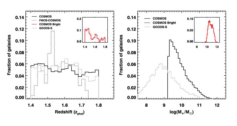
Figure 1: Properties of the photometric samples. Left: The solid black and grey histograms show the photometric redshift distributions of the SFGs we selected in COSMOS and GOODS-S, respectively. The black dotted histogram shows the FMOS-COSMOS spectroscopic redshift distribution of H$\alpha$ emitters. The histograms are normalized to the total number of objects in each sample . The red histogram in the inset shows the normalized distribution for a subsample of $750$ galaxies with predicted H$\alpha$ fluxes $\geq 2\times 10^{-16}$ erg cm^-2 s^-1 in COSMOS (Section 4). Right: Stellar mass distributions for the same COSMOS (black) and GOODS-S (grey) samples, and for the subsample of bright H$\alpha$ emitters in COSMOS (red histogram).

2 Data and sample selection

In this section, we introduce the photometric samples of SFGs drawn from the COSMOS and GOODS-S fields. We further present the FMOS-COSMOS spectroscopic survey dataset used to calibrate the predictions of H$\alpha$ fluxes, the latter being based on the star formation rates (SFRs) from SED fitting. Unless specified otherwise, the “COSMOS” and “GOODS-S photometric” samples will be treated separately and compared when possible. We will refer to the calibration dataset as the “FMOS-COSMOS” or the “spectroscopic” sample.

2.1 The COSMOS photometric sample

We selected the target sample from the latest COSMOS photometric catalog by Laigle et al. (2016), including the UltraVISTA-DR2 photometry. We identified star-forming galaxies according to the NUV-r, r-J criterion (Williams et al., 2009; Ilbert et al., 2013), and retained only the objects falling in the photometric redshift range $1.4<z<1.8$, resulting in a sample of $31,193$ galaxies with stellar masses of $M_{\star}\geq 10^{9.2}$ $M_{\odot}$. X-ray detected AGN from Civano et al. (2016) were flagged (PHOTOZ=9.99 in Laigle et al. 2016) and removed from our sample, since we could not reliably predict their line fluxes. We show the photometric redshift and the stellar mass distributions in Figure 1. The distribution of $z_{\rm phot}$ is flat in the redshift range we considered. On the other hand, the $M_{\star}$ distribution shows a substantial drop at $M_{\star}\sim 10^{9.2}$ $M_{\odot}$. The COSMOS sample is formally $\sim 90$% complete down to $M_{\star}\geq 10^{9.8}$ $M_{\odot}$ in this redshift range, corresponding to a cut at $K_{\mathrm{s}}=24$ mag in the shallowest regions covered by UltraVISTA (Laigle et al., 2016). However, Figure 1 shows that the completeness limit can be pushed to a lower value for the sample of SFGs we selected, simply because low mass galaxies are generally blue. In this case, this extended photometric sample allows for putting constraints on the number counts at low fluxes (Section 5), a regime usually inaccessible for purely spectroscopic analyses. Notice that we limit the number counts to a flux of $5\times 10^{-17}$ erg cm^-2 s^-1, above which the sample of H$\alpha$ emitters is virtually flux complete. Seventy-eight percent of the whole sample above this flux threshold have a stellar mass above the mass completeness limit, and this fraction rises to 95% for H$\alpha$ fluxes above $1\times 10^{-16}$ erg cm^-2 s^-1 used as a reference for the differential number counts in Section 5.2. Therefore, the results on the brightest tail of emitters are not affected by the drop of the stellar mass distribution in the sample.

We selected the $1.4<z<1.8$ redshift interval to match the one of the FMOS-COSMOS survey (Section 2.2). We adopted the stellar masses from the catalog by Laigle et al. (2016), computed with LePhare (Ilbert et al., 2006) and assuming Bruzual & Charlot (2003) stellar population synthesis models, a composite star formation history ($\mathrm{SFR}\propto\tau^{-2}te^{-t/\tau}$), solar and half-solar metallicities, and Calzetti et al. (2000) or Arnouts et al. (2013) extinction curves. We homogenized the IMFs applying a 0.23 dex correction to the stellar masses in the catalog, computed with the prescription by Chabrier (2003). We then re-modeled the SED from the rest-frame UV to the Spitzer/IRAC 3.6 $\mu$m band with the code Hyperz (Bolzonella et al., 2000), using the same set of stellar population models and a Calzetti et al. (2000) reddening law, but assuming constant SFRs. We chose the latter since they proved to reconcile the SFR estimates derived independently from different indicators and to consistently represent the main sequence of SFGs (Rodighiero et al., 2014). We checked the resulting SFRs and dust attenuation $A_{\rm V}$ from SED modeling against estimates from the luminosity at 1600 Å only (Kennicutt, 1998) and UV $\beta$-slope (Meurer et al., 1999). In both cases, we obtain consistent results within the scatter and the systematic uncertainties likely dominating these estimates. A tail of $\sim 8$% of the total COSMOS sample shows SFRs(UV)$\sim 0.15$ dex lower than SFR(SED), but at the same time they exhibit $A_{\rm V}$(UV)$\sim 0.1$ mag lower than $A_{\rm V}$(SED). However, these objects do not deviate anyhow appreciably from the distribution of predicted H$\alpha$ fluxes computed in Section 3, nor in stellar masses or photometric redshifts, as confirmed by a Kolmogorov-Smirnov test. We, thus, retain these galaxies in the analysis. SFRs derived from the rest-frame UV range only and dust extinctions from the modeling of the full SED extended to the Spitzer/IRAC $3.6$ $\mu$m band proved to robustly predict H$\alpha$ fluxes, not requiring any secondary corrections. We adopt these estimates in the rest of this work.

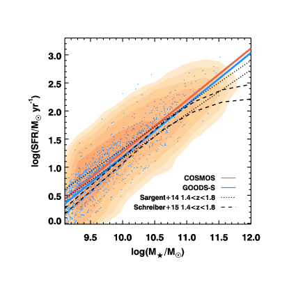
Figure 2: Main sequence of star forming galaxies at $z\sim 1.5$. Orange contours mark density contours of our sample of NUVrJ-selected SFGs at $1.4<z<1.8$ and with $M_{\star}\geq 10^{9.2}$ $M_{\odot}$ from the COSMOS field. Objects similarly selected and modeled in GOODS-S are indicated with blue points (Pannella et al., private communication). Best fit to the COSMOS and GOODS-S data are shown with orange and blue solid lines, respectively. Analytical parametrizations of the MS by Sargent et al. (2014) and Schreiber et al. (2015) for $z=1.4$ and $z=1.8$ are marked by dotted and dashed dark lines, respectively.

2.1.1 A control sample in GOODS-South

We further check the consistency of our compilation of stellar masses and SFRs in COSMOS comparing it with a sample of SFGs in GOODS-S. This field benefits from a deeper coverage of the rest-frame UV range, allowing for a better constraint of the SFRs down to lower levels, and to put constraints on the tail of H$\alpha$ emitters at low fluxes and masses, not recoverable in COSMOS. We, thus, selected a sample of $3,858$ galaxies with $M_{\star}\geq 10^{7.5}$ $M_{\odot}$ at $1.4<z<1.8$ applying the same criteria listed above. The $90$% mass completeness limit is $M_{\star}=10^{9}$ $M_{\odot}$ and $1,813$ galaxies fall above this threshold. We show the normalized redshift and stellar mass distribution of the GOODS-S in Figure 1. A two-tail Kolmogorov-Smirnov test shows that the redshift distributions are compatible. The different mass completeness limits between COSMOS and GOODS-S are evident from the right panel, with a tail of GOODS-S objects extending below $M_{\star}=10^{9}$ $M_{\odot}$. A Kolmogorov-Smirnov test on the raw data shows that the distributions are consistent with the hypotesis of being drawn from the same parent sample, especially when limiting the analysis to the COSMOS mass completeness threshold. We then modeled the SEDs of objects in GOODS-S applying the same recipes we adopted for the COSMOS sample (Pannella et al., private communication). As shown in Figure 2, we consistently recover the MS of galaxies in COSMOS and GOODS-S. We also find a good agreement with the analytical parametrizations of the MS by Sargent et al. (2014) and Schreiber et al. (2015).

2.2 The FMOS-COSMOS survey

The FMOS-COSMOS survey is a near infrared spectroscopic survey designed to detect H$\alpha$ and [N ii]$\lambda\lambda 6549,6584$ Å in galaxies at $1.43<z<1.74$ in the H band with the Fiber Multi-Object Spectrograph (FMOS, Kimura et al., 2010) on the Subaru Telescope. An integration of five hours allows for the identification of emission lines of total flux down to $4\times 10^{-17}$ erg cm^-2 s^-1 at $5\sigma$ with the H-long grism ($R\sim 2600$). Galaxies with positive H$\alpha$ detections have been re-imaged with the J-long grism ($R\sim 2200$) to detect [O iii]$\lambda\lambda 4959,5007$ Å and H$\beta$ emission lines to characterize the properties of the ionized interstellar medium (ISM, Zahid et al., 2014; Kashino et al., 2017a). For a detailed description of the target selection, observations, data reduction, and the creation of the spectroscopic catalog, we refer the reader to Silverman et al. (2015). For the scope of this work, i.e., the calibration of the H$\alpha$ fluxes predictions from the photometry, we selected only the objects with a signal-to-noise ratio $\geq 5$ on the observed H$\alpha$ flux. Their spectroscopic redshifts distribution is consistent with the one of photometric redshifts of the COSMOS sample discussed in Section 2.1 (Figure 1). We mention here that the primary selection relies on H$\alpha$ flux predictions based on continuum emission similar to the ones reported in the next section. This strategy might result in a bias against starbursting sources with anomalously large line EWs, strongly deviating from the average stellar mass, SFR, and extinction trends. While this is unlikely to affect the most massive galaxies, given their large dust content, we could miss starbursting galaxies at the low mass end ($M_{\star}\lesssim 10^{9.5}$ $M_{\odot}$), where the survey is not complete (Section 6.3). Moreover, since we preferentially targeted massive galaxies and J-band observations aimed at identifying the [O iii] emission followed a positive H$\alpha$ detection, we lack direct observational probe of sources with large [O iii]/H$\alpha$ ratios at low masses and H$\alpha$ fluxes. However, as we further discuss in Section 3.3, this potential bias is likely mitigated by the extrapolation of the analytical form we adopt to model the line ratios and predict [O iii] fluxes.

Note that $\sim 44$% of the initial FMOS-COSMOS targets were eventually assigned a spectroscopic redshift (Silverman et al., 2015). The success rate when predicting line fluxes and redshifts is likely higher considering that $\sim 25$% of the wavelength range is removed by the FMOS OH-blocking filter. The remaining failures can be ascribed to bad weather observing conditions; telescope tracking issues and fiber flux losses; high instrumental noise in the outer-part of the spectral range; errors on photometric redshifts (11% of objects are missed due to stochastic errors); the uncertainties on the dust content of galaxies; significant intra-population surface brightness variations. We also note that the misidentification of fake signal and/or non-H$\alpha$ line may occur in $\sim 10$% of the all line detections (Kashino et al., 2017b). The latter is a rough estimate based on $4$ discordant spectroscopic redshift between the FMOS-COSMOS and the zCOSMOS(-deep) surveys (Lilly et al., 2007) out of $28$ galaxies in common, assuming that the zCOSMOS determinations are correct. This line misidentification fraction may be overestimated, given the small sampling rate of zCOSMOS-deep at the range of the FMOS-COSMOS survey. Since we use the spectroscopic observations mainly to calibrate the flux predictions from photometry (Section 3), line misidentification does not strongly affect our results. In fact, either they cause flux predictions to be widely different from observations and, thus, they are excluded from the calibration sample (Figure 3); or, if by a lucky coincidence, the predicted H$\alpha$ fluxes fall close to the observed values of a different line, they spread the distribution of the observed-to-predicted flux ratios (Figure 3), naturally contributing to the final error budget we discuss later on. Notice also that the success rate increases up to $\sim 60$% for predicted H$\alpha$ fluxes $\geq 2\times 10^{-16}$ erg cm^-2 s^-1, a relevant flux regime further discussed in detail in the rest of the article.

3 Prediction of line fluxes from photometry

In this section we introduce the method we applied to predict the nebular line emission from the photometry of the samples presented above. The expected line fluxes are released in a publicly available catalog.

3.1 H$\alpha$ fluxes

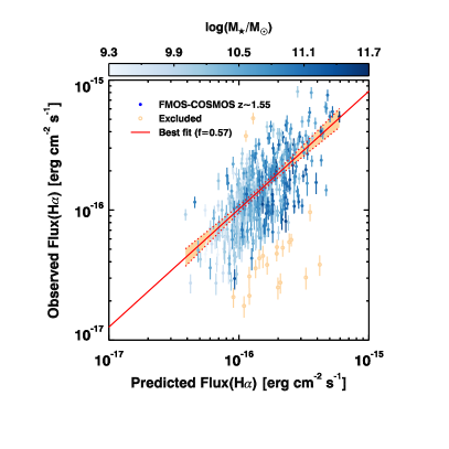
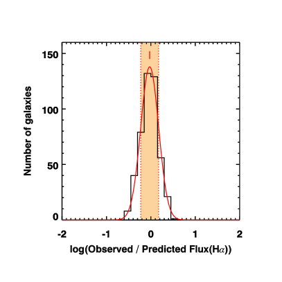
Figure 3: Prediction of total H$\alpha$ fluxes for star-forming galaxies in COSMOS. Left: Predicted and observed total, aperture corrected, H$\alpha$ fluxes for $486$ sources detected at $\geq 5\sigma$ in the spectroscopic follow-up with FMOS. Blue circles mark the $440$ sources used to optimize the $f$ value. Blue colors scale as the stellar mass. Orange empty circles represent sources with widely different predictions and observations, excluded from the calculation of the $f$ factor. The red solid and dotted lines represent the best fit to the logarithmic data and the associated $95$% confidence interval. Right: The black line shows the distribution of the observed-to-predicted H$\alpha$ flux ratios in logarithmic scale. The best gaussian fitting is overplot in red. The red tick and the orange shaded area mark the mean and the $1\sigma$ standard deviation of the best gaussian fit.

For each source in the photometric sample we computed the expected total observed H$\alpha$ flux based on SFRs and dust attenuation estimated in Section 2.1. We converted the SFR into H$\alpha$ flux following Kennicutt (1998), and we applied a reddening correction converting the $E_{\mathrm{star}}(B-V)$ for the stellar component into $E_{\mathrm{neb}}(B-V)$ for the nebular emission by dividing by $f=E_{\mathrm{star}}(B-V)/E_{\mathrm{neb}}(B-V)$. We computed $f$ minimizing a posteriori the difference between the observed and expected total H$\alpha$ fluxes from the FMOS-COSMOS survey presented in Kashino et al. (2017a). Therefore, here $f$ assumes the role of a fudge factor to empirically predict H$\alpha$ fluxes as close as possible to observations. Assigning a physical meaning to $f$ is prone to several uncertainties (Puglisi et al., 2016), and it is beyond the scope of this work. The minimization is based on $486$ galaxies in the spectroscopic sample with an observed H$\alpha$ flux $\gtrsim 2\times 10^{-17}$ erg cm^-2 s^-1 detected at $\geq 5\sigma$ (Figure 3). We verified that the value of $f$ is not biased by low SN detections or by a small subset of very bright sources, excluding objects in the 10^th and 90^th percentiles of the distribution of predicted H$\alpha$ fluxes. Moreover, the results do not change imposing $FLAG\geq 2$ and a lower signal-to-noise cut of $3$ on the observed H$\alpha$ fluxes from FMOS spectroscopy. Sources with divergent predictions and observations were excluded by applying a $2.5\sigma$ clipping on the ratios between observed and predicted H$\alpha$ fluxes, leaving $440$ galaxies available for the minimization procedure. These ratios are log-normally distributed, with a standard deviation of $0.19$ dex (Figure 3). The dispersion is widely dominated by the $\sim 50$% fiber losses and the ensuing uncertainties on the aperture corrections for the FMOS observations (Silverman et al., 2015). A $0.17$ dex dispersion is ascribable to this effect, while the remaining $0.1$ dex is partly intrinsic, due to the different star formation timescales traced by UV and H$\alpha$ light, and partly owing to the systematic uncertainties of the SED modeling.

Applying this technique, we obtain $f=0.57\pm 0.01$, with a scatter of 0.23. A consistent result is retrieved comparing the observed SFR(UV) and SFR(H$\alpha$) (Kashino et al., 2013). The value of $f$ is higher than the one normally applied for local galaxies ($f=0.44\pm 0.03$, Calzetti et al., 2000), consistently with recent results for high-redshift galaxies (Kashino et al., 2013; Pannella et al., 2015; Puglisi et al., 2016). Note that we estimated $E_{\mathrm{star}}(B-V)$ using the Calzetti et al. (2000) reddening law, while we adopted the Cardelli et al. (1989) prescription with $R_{\rm V}=3.1$ to compute $E_{\mathrm{neb}}(B-V)$, analogously to what reported in the original work by Calzetti et al. (2000), where they used the similar law by Fitzpatrick (1999). Using the Calzetti et al. (2000) reddening curve to compute both the stellar and nebular extinction would result in higher values of $f$ for local ($f=0.58$) and $z\sim 1.55$ galaxies ($f=0.76\pm 0.01$).

Adopting $f=0.57$, the best fit to the logarithmic data is $\rm{log(H\alpha_{obs})}=(0.91\pm 0.01)\,\rm{log(H\alpha_{pred})}+(-1.48\pm 0.19)$ with a correlation coefficient $\rho=0.9998$. The uncertainties represent the statistical error in the fitting procedure, while the scatter of the relation is $\sigma=0.19$ dex (Figure 3). Assuming a fixed slope of 1, the best fit is $\rm{log(H\alpha_{obs})}=\rm{log(H\alpha_{pred})}+(-0.009\pm 0.002)$. Secondary corrections as a function of $M_{\star}$ or $E(B-V)$ are not necessary, since the $\rm{log(H\alpha_{obs}/H\alpha_{pred})}$ ratio is constant and consistent with 0 over the ranges probed by the FMOS-COSMOS detections ($10^{9.3}\leq M_{\star}\leq 10^{11.7}$ $M_{\odot}$, $E(B-V)\leq 0.84$ mag). Eventually, we adopted $f=0.57$ to predict the H$\alpha$ and other line fluxes (see below) both in COSMOS and GOODS-S, assuming its validity over the entire stellar mass and reddening ranges covered by these samples. We also assume that the uncertainties on the predicted H$\alpha$ fluxes derived for the FMOS-COSMOS sample are applicable for galaxies in GOODS-S. In Figure 4 we show the correlations among the predicted H$\alpha$ fluxes and the SED-derived stellar masses, SFRs, and reddening $E(B-V)$ for the COSMOS and GOODS-S photometric samples. We also plot the spectroscopically confirmed objects from the FMOS-COSMOS survey. The large $E(B-V)$ at high stellar masses compensates the increase of the SFR on the Main Sequence, so that the $M_{\star}$ - observed H$\alpha$ flux relation is flat above $M_{\star}\sim 10^{10}$ $M_{\odot}$, ensuring high stellar mass completeness above this threshold when observing down to H$\alpha$ fluxes of $1\times 10^{-17}$ erg cm^-2 s^-1. Notice that the FMOS-COSMOS observations are biased towards the lower $E(B-V)$, as expected from the initial selection (Section 2.2) and the fact that less dusty objects are naturally easier to detect. Finally, the uncertainties on $E(B-V)$ are included in the correlation of SFR into observed H$\alpha$ fluxes shown in the central panel.

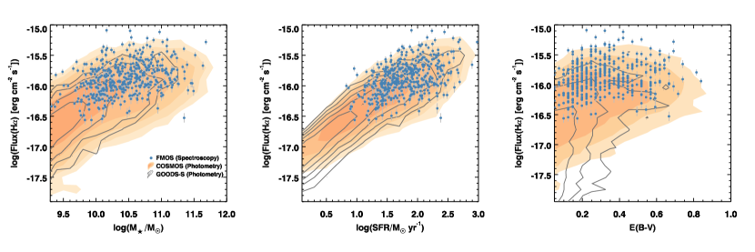
Figure 4: Predicted H$\alpha$ fluxes as a function of SED derived quantities. The orange and grey contours show the density contours of the COSMOS and GOODS-S photometric samples, respectively. The blue points mark the position of spectroscopically confirmed objects in the FMOS-COSMOS survey. The H$\alpha$ fluxes are integrated and not corrected for reddening. Left: Stellar mass vs H$\alpha$ fluxes. Centre: SFR vs H$\alpha$ fluxes. Right: $E(B-V)$ vs H$\alpha$ fluxes.

3.2 H$\beta$ fluxes

We computed H$\beta$ fluxes rescaling the H$\alpha$ values for the different extinction coefficients $k_{\lambda}$ and assuming the intrinsic ratio $\rm{H}\beta=\rm{H}\alpha/2.86$ (Osterbrock & Ferland, 2006). Note that the stellar Balmer absorption might impact the final observed H$\beta$ flux. We, thus, compute a stellar mass dependent correction following Kashino et al. (2017a):

$$f_{\mathrm{corr}}=\mathrm{max}[1,1.02+0.30\,\mathrm{log}(M_{\star}/10^{10}\,M_{\odot})]$$ (1)

where $f_{\mathrm{corr}}$ corresponds to a correction up to $50$%. We report this term in the released catalog for completeness so to compute the observed, Balmer-absorbed fluxes, if needed. However, the correction is not applied to the total H$\beta$ fluxes shown in the rest of this work.

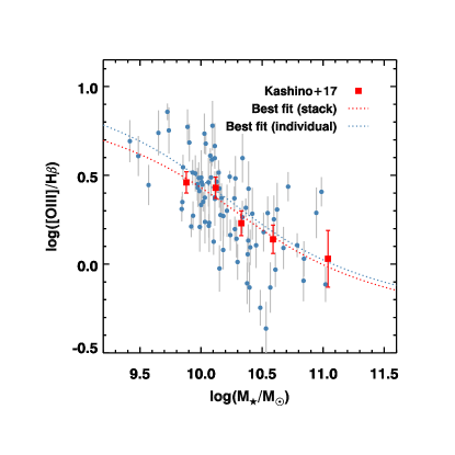
Figure 5: [OIII]/H$\beta$ ratio as a function stellar mass for the FMOS-COSMOS survey at $z\sim 1.5$. Blue points mark the observed galaxies in the FMOS-COSMOS survey with $3\sigma$ detections of both the [O iii] and H$\beta$ lines. Grey error bars represent the $1\sigma$ uncertainties on the ratio estimates. Red squares mark the average values for SFGs in the FMOS-COSMOS survey as derived in Kashino et al. 2017a. The red and blue lines indicate the best fit to the stacked values and individual sources, respectively.

3.3 [OIII] fluxes

We predict [O iii] fluxes adopting a purely empirical approach calibrated against the average spectra of the FMOS-COSMOS SFGs described in Kashino et al. (2017a). The observed $\rm{log}$([O iii]$/$H$\beta$) ratio anticorrelates with $\rm{log}(M_{\star})$, as shown in Figure 5 (Mass-Excitation diagram, Juneau et al., 2011). Being close in wavelength, this line ratio is not deeply affected by reddening corrections. Here we predict [O iii] fluxes from H$\beta$ forcing the line ratio to follow a simple arctangent model fitting the stacked values. The best fit model is: $\rm{log}$([O iii]$/$H$\beta$$)=(0.30\pm 0.37)+(0.48\pm 0.12)\,\mathrm{arctan}\{-[\mathrm{log}(M_{\star}/M_{\odot})-(10.28\pm 0.84)]\}$. Fitting the individual sources does not impact the main conclusions of this work. Note that these predictions are valid only for the redshift window $1.4<z<1.8$, where a significant evolution of the [O iii]/H$\beta$ ratio is not expected (Cullen et al., 2016). Notice also that the number of secure individual $3\sigma$ detections of both [O iii] and H$\beta$ is restrained ($84$ galaxies) and that the line ratio suffers from a significant scatter.

The comparison between predicted and observed [O iii] fluxes is shown in Figure 6. The best fit to the logarithmic data is $\rm{log(}$[O iii]${}_{\mathrm{obs}})=(1.00\pm 0.03)\,$ $\rm{log(}$[O iii]${}_{\mathrm{pred}})+(0.08\pm 0.45)$ with a correlation coefficient $\rho=0.99995$. The best model is derived from $181$ galaxies with a $\geq 3\sigma$ detection of [O iii] from our FMOS-COSMOS sample, after applying a $2\sigma$ clipping to remove $22$ strong outliers. Note that the flux range covered by FMOS [O iii] observations is more limited than for H$\alpha$. The distribution of observed-to-predicted [O iii] fluxes has a width of $\sigma=0.25$ dex, dominated by the uncertainties on FMOS aperture corrections, as for the H$\alpha$ line. Figure 7 shows that we underpredict the [O iii] flux by up to $\sim 0.1$ dex for galaxies with low SFR ($\lesssim 30$ $M_{\odot}$ yr^-1) and low $A_{\rm V}$ ($\lesssim 0.8$ mag) from the SED fitting, but we do not find any evident dependence on stellar mass, even if FMOS-COSMOS [O iii] observations probe only the $M_{\star}\gtrsim 10^{9.5}$ $M_{\odot}$ regime. Since we allowed for a lower signal-to-noise ratio to detect [O iii] emission than H$\alpha$ fluxes in order to increase the sample statistics, here we adopted a stricter clipping threshold to eliminate outliers. In particular, AGN contamination likely boosts [O iii] fluxes in the latter, massive objects (median $M_{\star}=10^{10.8}$ $M_{\odot}$), causing systematically larger observed fluxes than predicted for inactive SFGs. We applied the same calibration to the galaxies in GOODS-S, and assumed that the uncertainties derived from the spectroscopic sample in COSMOS applies to GOODS-S, too. Note that the [O iii] flux and the [O iii]/H$\beta$ ratio are sensitive to the presence of AGN. Moreover, the number of bright [O iii] emitters with low masses is significantly larger than for the H$\alpha$ line, since the [O iii]/H$\beta$ increases for decreasing masses. This is particularly relevant for the GOODS-S sample. As mentioned in Section 2.2, the FMOS-COSMOS survey does not probe the low-mass, high [O iii]/H$\beta$ regime, where line ratios up to $0.8-1$ are typically observed (Henry et al., 2013). However, extrapolating the best fit models shown in Figure 5 down to $M_{\star}\sim 10^{8}$ $M_{\odot}$, we cover the range of observed ratios, likely mitigating a potential bias against large [O iii] fluxes.

3.4 [OII] fluxes

[O ii] might be used as a SFR tracer (Kennicutt, 1998; Kewley et al., 2004; Talia et al., 2015), even if its calibration depends on secondary parameters such as the metal abundance. Here we simply assume $L($[O ii]$)=L($H$\alpha$$)$ (Kewley et al., 2004) and the extinction coefficient $k($[O ii]$)=4.771$ from the Cardelli et al. (1989) reddening curve ($R_{\rm V}=3.1$). In Figure 6 we show the predicted [O ii] fluxes against a sample of $43$ spectroscopic measurements in COSMOS from Kaasinen et al. (2017) in common with our catalog. After applying a $2\sigma$ clipping to the $\rm{[OII]_{obs}/[OII]_{pred}}$ flux ratios, the best fit to the relation between these two quantities is $\rm{log([OII]_{obs})}=(0.95\pm 0.06)\,\rm{log([OII]_{pred})}+(-0.83\pm 0.92)$, with a correlation coefficient $\rho=0.99996$. The width of the distribution of the ratios $\rm{[OII]_{obs}/[OII]_{pred}}$ is $\sigma\sim 0.22$ dex. We applied the same method to the sample in GOODS-S. Also in this case, the stricter clipping threshold than for H$\alpha$ fluxes (Section 3.1) compensates for the lower signal-to-noise limit allowed for [O ii] detections, so to increase the size of the available sample. Applying a $5\sigma$ detection threshold and a $2.5\sigma$ clipping to [O ii] observed fluxes results in a similar final object selection to the one presented above.

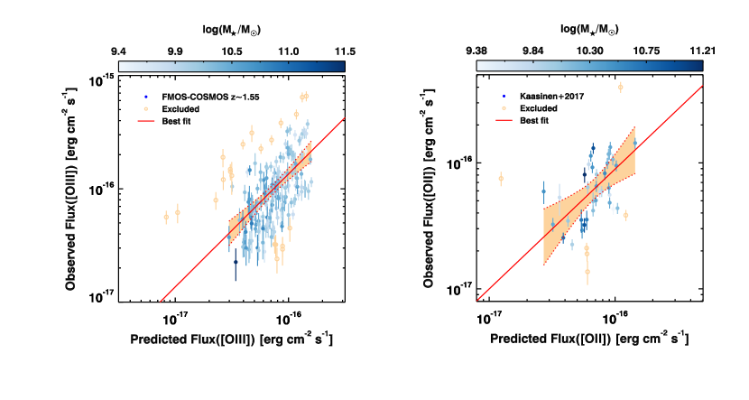
Figure 6: Oxygen lines flux predictions. Left: Blue circles mark predicted and observed [O iii] fluxes from a sample of $159$ galaxies with $3\sigma$ detections in the FMOS-COSMOS survey. Symbols are color coded according to stellar masses. The red solid line and orange shaded area indicate the best fit to the data and its $95$% confidence interval. Orange empty circles have been excluded from the fit. Right: Blue circles mark predicted and observed [O ii] fluxes from a sample of $37$ galaxies with $3\sigma$ detections from Kaasinen et al. 2017. Symbols are color coded according to stellar masses. The red solid line and orange shaded area indicate the best fit to the data and its $95$% confidence interval. Orange empty circles have been excluded from the fit.

We note that a similar approach was applied by Jouvel et al. (2009) to simulate emission lines for a mock sample of objects based on the observed SEDs of galaxies in COSMOS. In their work, Jouvel et al. (2009) based the flux predictions assuming [O ii] as a primary tracer of SFR and on a set of fixed line ratios. However, [O ii] shows secondary dependencies on other parameters such as metallicity, even if in first approximation it traces the current SFR. Moreover, the line ratios significantly change with redshift. Furthermore, a proper treatment of the dust extinction is fundamental to derive reliable nebular line fluxes, introducing a conversion between the absorption of the stellar continuum and of the emission lines. Here we exploited the updated photometry in the same field and GOODS-S, and we tied our predictions to direct spectroscopic observations of a large sample of multiple lines in high-redshift galaxies, the target of future surveys. We primarily estimated the H$\alpha$ fluxes, a line directly tracing hydrogen ionized by young stars and brighter than [O ii], thus accessible for larger samples of galaxies spanning a broader range of SFRs and masses. Predictions for oxygen lines emission were directly compared to observations as well.

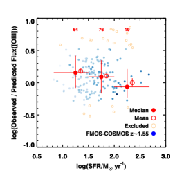
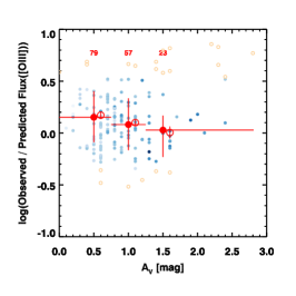
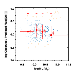
Figure 7: Observed-to-predicted [O iii] flux ratios as a function of SED-derived quantities. In each panel, blue filled circles show the [O iii]_obs/[O iii]_pred ratios against SED-derived SFRs (left), $A_{\rm V}$ (center), and stellar masses $M_{\star}$ (right) for the sample of galaxies with an [O iii] flux measurement from the FMOS-COSMOS survey. Symbols are color coded according to stellar masses as in Figure 6. Orange empty circles have been excluded applying the $2\sigma$-clipping described in Section 3.3. The red filled circles and vertical bars represent the median of [O iii]_obs/[O iii]_pred ratios in subsequent bins and the $\pm 1\sigma$ percentiles ($15.84$, $84.16$%). The horizontal bars show the width of each bin, selected based on the enclosed number of objects (reported in red in the three panels) and the typical systematics affecting SED modeling. Red open circles and bars represent the mean of line ratios in each bin and its standard error ($=\sigma/\sqrt{N}$), where $N$ is the number of objects per bin.

4 A sample of bright H$\alpha$ emitters at z$\,\sim 1.5$

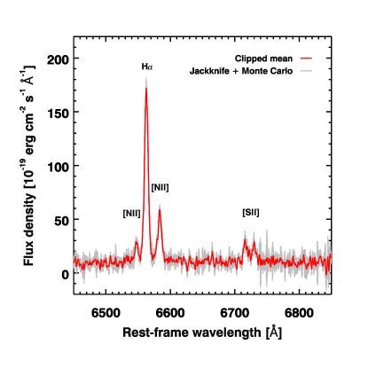
Figure 8: Average spectrum of bright H$\alpha$ emitters from the FMOS-COSMOS survey. The red line marks the clipped average spectrum of $135$ individual line emitters with aperture corrected, observed H$\alpha$ fluxes $\geq 2\times 10^{-16}$ erg cm^-2 s^-1from the catalog by Kashino et al. (2017a). The grey line shows the associated uncertainty estimated with Monte Carlo and Jackknife techniques.

The sensitivity to emission lines achieved by the FMOS-COSMOS and similar spectroscopic surveys is an order-of-magnitude deeper than what expected for forthcoming large surveys (i.e., Euclid wide survey: $\geq 2\times 10^{-16}$ erg cm^-2 s^-1, $3.5\sigma$; WFIRST: $\geq 0.5-1\times 10^{-16}$ erg cm^-2 s^-1 for extended sources, $3\sigma$, Figure 2-15 of Spergel et al. 2015). Therefore, the physical characterization of the population of bright H$\alpha$ emitters is a key feature in the current phase of preparation for these missions. Here we have the opportunity to achieve this goal for a fairly large sample of galaxies, exploiting both photometric and spectroscopic data.

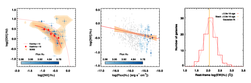
Figure 9: Spectroscopic properties of bright H$\alpha$ emitters at $z\sim 1.5$. Left: BPT diagram for spectroscopically confirmed emitters with H$\alpha$ flux $\geq 2\times 10^{-16}$ erg cm^-2 s^-1 from the FMOS-COSMOS survey. The blue solid circles mark bright emitters. The color intensity scales as the H$\alpha$ flux in units of $10^{-16}$ erg cm^-2 s^-1 reported in the color bar. The red diamonds and solid line mark the average location of the FMOS-COSMOS sample of SFGs with total H$\alpha$ flux $\geq 4\times 10^{-17}$ erg cm^-2 s^-1 and the best fit by Kashino et al. (2017a). The red dotted line indicates the limiting curve dividing SFGs and AGN at $z=1.55$ as parametrized in Kewley et al. (2013). The orange shaded area marks the location of SDSS galaxies with an intrinsic H$\alpha$ luminosity corresponding to a total H$\alpha$ flux of $\geq 4\times 10^{-17}$ erg cm^-2 s^-1 at $z=1.55$. Centre: [N ii]/H$\alpha$ ratios as a function of the total observed H$\alpha$ flux for the spectroscopic FMOS-COSMOS sample. The blue solid circles mark bright H$\alpha$ emitters in the BPT in the left panel. The color intensity scales as the H$\alpha$ flux in units of $10^{-16}$ erg cm^-2 s^-1 reported in the color bar. Grey dots and arrows mark the position of the rest of the FMOS-COSMOS spectroscopic sample described in Kashino et al. (2017a). The red solid line indicates the best fit to the data. The orange area and the red dotted lines mark the $95$% confidence limits of the fit. Right: The red histogram shows the distribution of rest-frame $\rm{log}[$EW$($H$\alpha)]$ for spectroscopically confirmed emitters with H$\alpha$ flux $\geq 2\times 10^{-16}$ erg cm^-2 s^-1. The red dotted line marks the best Gaussian fit to the distribution. The orange band indicates the $1\sigma$ confidence limit around the value estimated from the stacked spectrum in Figure 8.

4.1 Spectroscopy: line ratios and equivalent widths

The general spectroscopic properties of the FMOS-COSMOS sample are detailed in Kashino et al. (2017a). Here we focus on a subset of $135$ bright sources with total, observed (i.e., corrected for aperture effects, but not for extinction) H$\alpha$ fluxes $\geq 2\times 10^{-16}$ erg cm^-2 s^-1 from their catalog. First, we visually inspected and manually re-fitted the FMOS spectra of these sources. We, then, stacked the individual spectra, applying a $5\sigma$ clipping at each wavelength. The clipping does not introduce evident biases: the resulting spectrum is fully consistent both with an optimally weighted average and a median spectrum. The average spectrum and the associated uncertainty, estimated through Jackknife and Monte Carlo techniques, are shown in Figure 8. From this spectrum we derived H$\alpha$, [N ii], [S ii]$\lambda\lambda 6717,6731$ Å, and continuum emission fluxes for the population of bright emitters. Note that [S ii] lines are not in the observed wavelength range for galaxies at $1.67<z<1.74$.

The left panel of Figure 9 shows the BPT diagram for a subsample of $39$ bright emitters in the FMOS-COSMOS sample with coverage of H$\beta$ and [O iii]. The bright emitters at lower [N ii]/H$\alpha$ ratios are mainly distributed around the average locus of the FMOS-COSMOS sample down to the detection limit of $\geq 4\times 10^{-17}$ erg cm^-2 s^-1 (Kashino et al., 2017a). At ratios above log([N ii]/H$\alpha$)$\gtrsim-0.5$, bright H$\alpha$ emitters show higher [O iii]/H$\beta$ ratios, possibly due to contamination by AGN, which dominate the line emission in some extreme cases. However, there are not evident trends between the position in the BPT and the H$\alpha$ flux of these bright emitters, as shown by the color bar. The sample is also offset with respect to the average locus of a sample of $6,638$ low-redshift galaxies ($0.04<z<0.2)$ selected from the Sloan Digital Sky Survey DR7 (Abazajian et al., 2009) with well-constrained [O iii]/H$\beta$ and [N ii]/H$\alpha$ ratios (Juneau et al., 2014) and with an intrinsic H$\alpha$ luminosity corresponding to fluxes $\geq 4\times 10^{-17}$ erg cm^-2 s^-1 at $z=1.55$. This shows that the offset in the BPT diagram is not merely due to selection effects (Juneau et al., 2014; Kashino et al., 2017a). Nine out of $39$ emitters ($\sim 23$%) are classified as AGN according to the criterion by Kewley et al. (2013) at $z\sim 1.55$, and this partly results from the selection of Chandra detected sources to complement the main color selection for the FMOS-COSMOS survey (Silverman et al., 2015). In Figure 9 we show how log([N ii]/H$\alpha$) apparently anticorrelates with observed H$\alpha$ fluxes. The best fit is log([N ii]/H$\alpha$)$=(-0.22\pm 0.02)\rm{log(H\alpha)}-(3.90\pm 0.26)$ (correlation coefficient $\rho=0.99983$). However, this correlation is naturally affected by observational biases and disappears when stacking [N ii] non-detections (Kashino et al., 2017a). The mean ratio log([N ii]/H$\alpha$) of the subsample of $91$ sources with [N ii] $3\sigma$ detections is log([N ii]/H$\alpha$)$=-0.47\pm 0.02$, compatible with the value obtained from the stacked spectrum of the whole sample of $135$ bright spectroscopic emitters (log([N ii]/H$\alpha$)$=-0.52\pm 0.01$). Finally, we computed the distribution of rest-frame equivalent widths of H$\alpha$ (EW(H$\alpha$)) and its mean (Figure 9), obtaining log[EW(H$\alpha$)/Å]$=2.08\pm 0.03$, similar to the result from stacking (log[EW(H$\alpha$)/Å]$=2.05\pm 0.01$). Adopting the median, a gaussian model of the distribution, or a $3\sigma$-clipped average does not impact the results. These values are consistent with recent compilations of high-redshift galaxies at similar masses (i.e., Fumagalli et al., 2012; Mármol-Queraltó et al., 2016).

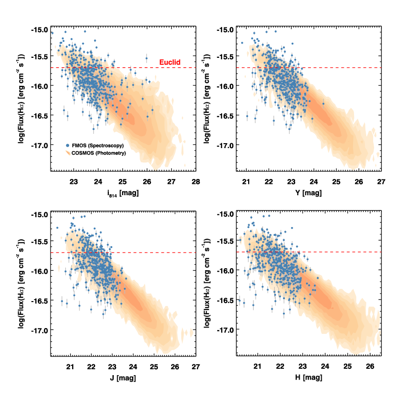
Figure 10: Photometric properties of the COSMOS sample of star-forming galaxies at $z\sim 1.5$. The panels show the relation between the H$\alpha$ fluxes and the HST/ACS i band (top left), Y band (top right), J band (bottom left), and H band (bottom right) magnitudes from UltraVISTA-DR2. Orange contours represent the whole photometric COSMOS sample and the predicted H$\alpha$ fluxes. Blue points indicate the subset of objects confirmed by FMOS and their spectroscopic H$\alpha$ fluxes. Grey bars mark the $1\sigma$ uncertainties on the observed H$\alpha$ fluxes. The red dashed line marks the limit of $2\times 10^{-16}$ erg cm^-2 s^-1 expected for the Euclid wide survey.

4.2 Optical and near-IR photometry

The tail of bright H$\alpha$ emitters from the FMOS-COSMOS sample is fairly bright in the observed optical and near-IR bands. In Figure 10 we show the relation between the H$\alpha$ fluxes and HST/ACS i₈₁₄, and the UltraVISTA-DR2 Y, J, H band MAG_AUTO magnitudes for the COSMOS photometric sample (Laigle et al., 2016) and the subset of objects spectroscopically confirmed with FMOS. For reference, the emitters with expected H$\alpha$ fluxes $\geq 2\times 10^{-16}$ erg cm^-2 s^-1 in the COSMOS field have $H<22.5$ mag. The contours representing the whole photometric sample of SFGs in COSMOS show that our flux predictions capture the scatter of the spectroscopic observations, while correctly reproducing the slope of the relations in each band. Note that, by construction, the FMOS-COSMOS selection prioritizes bright galaxies to ensure a high detection rate of emission lines.

4.3 Rest-frame UV sizes

We further attempted to estimate the typical sizes of bright H$\alpha$ emitters. In order to increase the statistics of bright emitters and not to limit the analysis to spectroscopically confirmed objects, we selected a subsample of $750$ SFGs in COSMOS with predicted H$\alpha$ fluxes $\geq 2\times 10^{-16}$ erg cm^-2 s^-1 ($2$% of the total photometric sample). The insets in Figure 1 show the normalized distributions of photometric redshifts and stellar masses for this subsample. Bright emitters follow the same redshift distribution of the whole population, while being fairly massive ($\langle\rm{log}(M_{\star}/M_{\odot})\rangle=10.7\pm 0.4$). Note that all bright emitters in COSMOS lie well above the stellar mass completeness threshold. This is consistent with the fact that we do not find any SFG on the main sequence in GOODS-S with a predicted H$\alpha$ flux $\geq 2\times 10^{-16}$ erg cm^-2 s^-1 at any mass below our COSMOS completeness limit of $M_{\star}=10^{9.8}$ $M_{\odot}$.

Since we do not have direct access to the spatial distribution of the H$\alpha$ flux, we measured the sizes in the HST/ACS i₈₁₄ band, corresponding to rest-frame $\sim 3100$ Å at $z=1.55$. Note that given the result on $f$, the attenuation of H$\alpha$ and in the i₈₁₄ band are expected to be nearly identical. We present the analysis for the $750$ emitters with predicted H$\alpha$ flux $\geq 2\times 10^{-16}$ erg cm^-2 s^-1, but the results do not change if we consider only the spectroscopic subsample from the FMOS-COSMOS survey. First, we extracted $15"\times 15"$ cutouts from the COSMOS archive and we visually inspected them. Considering that the area covered by the HST/ACS follow-up is smaller than the whole COSMOS field and excluding strongly contaminated sources, we worked with $649$ objects in total. We show a collection of the latter in Appendix A. Given their clumpy morphology, we recentered the cutouts on the barycenter of the light found by SExtractor (Bertin & Arnouts, 1996), allowing for a small fragmentation and smoothing over large scales. The final results do not change if we center the images on the peak of the light distribution. We, then, stacked the cutouts computing their median to minimize the impact of asymmetries and irregularities. We finally measure the effective radius with a curve-of-growth, obtaining $R_{\rm e}=(0.48\pm 0.01)$ arcsec ($\sim 4$ kpc at $z=1.55$, Figure 11). The uncertainty is obtained bootstrapping $1,000$ times the stacking procedure and extracting the curve of growth. To confirm this estimate, we used GALFIT (Peng et al., 2010a) to model the 2D light distribution with a Sersić profile, leaving all the parameters free to vary. To extract a meaningful size directly comparable with the previous estimate, we measured the effective (half-light) radius of the PSF-deconvolved profile, obtaining $R_{\rm GALFIT}=0.46"$. The $R_{\rm e}$ value is comparable with the effective radius of star-forming galaxies on the average mass-size relations in literature (i.e., median circularized $R_{\mathrm{e,circ}}=3.4-3.0$ kpc, semi-major axis $R_{\mathrm{semi-major}}\sim 4.7-4.1$ kpc for late-type galaxies with $\rm{log}(M_{\star}/M_{\odot})=10.75$ at $z=1.25-1.75$, van der Wel et al. 2014).

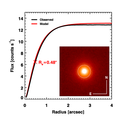
Figure 11: Median HST/ACS $i_{814}$ image of bright H$\alpha$ emitters and its curve of growth. The black line represents the curve-of-growth of the median image of $649$ galaxies from the FMOS-COSMOS survey with predicted H$\alpha$ fluxes $\geq 2\times 10^{-16}$ erg cm^-2 s^-1. The red line shows the result of the 2D light decomposition with GALFIT, including the deconvolution of the PSF. The red cross marks the effective radius. The inset shows the $3.75"\times 3.75"$ median stacked image. The white circle indicates the effective radius $R_{\rm e}=0.48"$. It also roughly corresponds to the “optimal” aperture size maximizing the signal-to-noise ratio for the detection ($R=0.43"$, Section 6.4).

5 Number counts of line emitters

We compute the projected cumulative number counts of line emitters at $z\sim 1.5$ starting from the photometric samples in COSMOS and GOODS-S. We base the counts on the predicted H$\alpha$, [O iii], and [O ii] fluxes as detailed above. Then, we model the evolution of the number counts of H$\alpha$ emitters with cosmic time, a crucial step in preparation of forthcoming large spectroscopic surveys with Euclid (Laureijs, 2009) and WFIRST (Green et al., 2012; Spergel et al., 2015). Our method has the advantage of fully exploiting the large number statistics of current photometric surveys and it complements the classical approach based on a spectroscopic dataset and the modeling of the evolution with redshift of the H$\alpha$ luminosity functions (Geach et al., 2010; Pozzetti et al., 2016). A detailed analysis of the H$\alpha$ LF for the FMOS-COSMOS survey is deferred to future work (Le Fèvre et al. in prep.)

5.1 H$\alpha$ emitters: the FMOS-COSMOS redshift range

First, we computed the cumulative number counts for the redshift range $1.4<z<1.8$ covered by the FMOS-COSMOS survey, starting from the COSMOS and GOODS-S photometric samples spread over an area of $1.57$ deg² and $0.054$ deg², respectively. The cumulative number counts are reported in Table 1 and shown in Figure 12. We computed the uncertainties on the cumulative counts both as Poissonian $68$% confidence intervals and from simulations. In order to capture the sample variance, we bootstrapped 1,000 mock samples of the same size of the observed one, randomly extracting objects from the photometric samples, allowing for any number of duplicates. We, then, recomputed the number counts for each mock sample and estimated the uncertainties as the standard deviation of their distribution for each flux. We further simulated the impact of the cosmic variance on small angular scales counting galaxies in areas of 0.26 deg² ($1/6$ of the total surface covered by the COSMOS photometric sample) and $0.054$ deg², taken randomly in the COSMOS field. We, then, added these contributions in quadrature.

Furthermore, we included the effect of the uncertainties on the predicted H$\alpha$ fluxes on the final estimate of the number counts, as necessary to fairly represent their scatter. These uncertainties naturally spread out the counts in a flux bin to the adjacent ones. In presence of an asymmetric distribution of galaxies in the flux bins, this causes a net diffusion of objects in a specific direction: in this case, from low towards high fluxes. This happens because of the negative, steep slope reached in the brightest flux bins, simply meaning that there are many more emitters at low fluxes than at the high ones. Neglecting the uncertainties on the predicted fluxes would, thus, result in an underestimate of the number counts at high fluxes, since the low-flux population dominates over the bright tail. Note that this is relevant in our calculations, given the relatively large uncertainty also in the brightest flux tail, while this is generally not an issue for well determined total fluxes (i.e., with narrow-band imaging or, in principle, grism spectroscopy, but see Section 6.4). The typical flux error is $\sigma_{\rm pred}=0.1$ dex, obtained subtracting in quadrature the error associated with the total observed H$\alpha$ flux from FMOS-COSMOS ($\sigma_{\rm obs}=0.17$ dex, dominated by aperture corrections) from the dispersion of the distribution of $\rm{H\alpha_{obs}/H\alpha_{pred}}$ flux ratios ($\sigma=0.19$ dex, Figure 3). Uncertainties related to SED modeling and intrinsic scatter both contribute to this dispersion (Section 3.1). To simulate the diffusion of galaxies from low to high fluxes, we convolved the counts per flux bin with a Gaussian curve of fixed width $\sigma_{\rm broad}$ in the logarithmic space, renormalizing for the initial counts per flux bin. Finally, we recomputed the cumulative counts, now broadened by the errors on predicted fluxes. Adopting the most conservative approach, we set $\sigma_{\rm broad}=0.19$ dex, as if all the dispersion of the distribution of $\rm{H\alpha_{obs}/H\alpha_{pred}}$ were due to the uncertainty on $\rm{H\alpha_{pred}}$. This procedures returns a strong upper limit on the cumulative number count estimate, increasing the original values for the COSMOS photometric sample by a factor of $\sim 3$ at H$\alpha$ fluxes of $3\times 10^{-16}$ erg cm^-2 s^-1, as shown in Figure 12. In the same figure we show the results of an identical analysis applied to the GOODS-S photometric sample, along with the modeling of the recent compilation of spectroscopic and narrow-band data and LFs by Pozzetti et al. (2016). All the curves refer to the same redshift range $1.4<z<1.8$. The counts for the COSMOS and GOODS-S samples are fully consistent within the uncertainties down to the COSMOS completeness flux limit of $5\times 10^{-17}$ erg cm^-2 s^-1. The deeper coverage of the rest-frame UV range available for GOODS-S allows us to extend the number counts to H$\alpha$ fluxes of $1\times 10^{-17}$ erg cm^-2 s^-1. Below these limits, the convolved number counts in the two fields are lower than the initial ones due to the incompleteness. The cumulative counts are broadly consistent with the empirical models by Pozzetti et al. (2016), collecting several datasets present in the literature. The agreement is fully reached when considering the effect the uncertainties on the flux predictions. In particular, our results best agree with Models 2 and 3, the latter being derived from high-redshift data only, revising the number counts towards lower values than previously estimated (Geach et al., 2010). Note that our selection includes only color-selected normal SFGs. Other potentially bright H$\alpha$ emitters, such as low-mass starbursting galaxies and AGN, might further enhance the final number counts (Section 6).

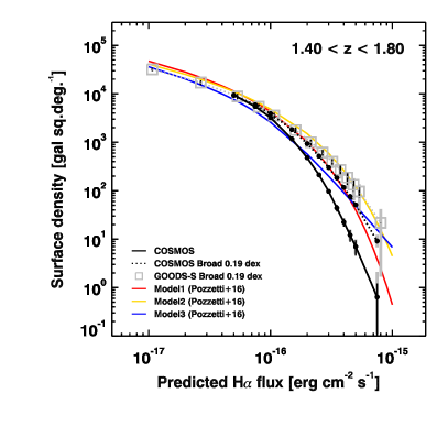
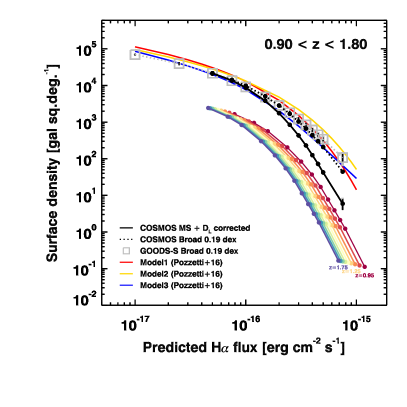
Figure 12: Cumulative H$\alpha$ counts. Left: Cumulative number counts in the redshift range $1.4<z<1.8$. The H$\alpha$ fluxes are predicted from the photometry. The solid black line marks the cumulative counts integrated over the full redshift range. Grey bars indicate the Poissonian $68$% confidence interval. Black bars show the $1\sigma$ uncertainty on cumulative counts from bootstrap and Monte Carlo simulations. The dotted black line marks the upper limit on cumulative counts, including the uncertainty on the predicted fluxes, causing a broadening of the original values. Grey squares and error bars show the upper limit on the cumulative counts for the GOODS-S photometric sample and their $1\sigma$ uncertainties. The red, golden, and blue solid lines mark Model 1, 2, and 3 by Pozzetti et al. (2016). Right: Cumulative number counts in the redshift range $0.9<z<1.8$ covered by the forthcoming Euclid mission. Colored lines mark the cumulative counts in $dz=0.1$ redshift slices (Section 5.2). Other lines and symbols follow the same scheme of the left panel. Note: The lower and upper (convolved, “broad”) counts can be obtained subtracting and adding the absolute error $\sigma_{\rm conv}$ to the “average” counts in Table 1.

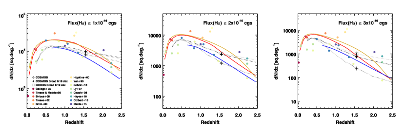
Figure 13: Differential H$\alpha$ counts. The dark grey empty star mark the differential counts $dN/dz$ from the photometric sample in COSMOS. The black filled star corresponds to the upper limit on the counts, including the uncertainty on the predicted fluxes. The light grey empty square indicates the upper limit on the counts for the GOODS-S sample. Grey vertical bars indicate the Poissonian $68$% confidence interval. Black bars show the $1\sigma$ uncertainty on cumulative counts from bootstrap and Monte Carlo simulations. The dark grey dotted line represents the $dN/dz$ counts for the COSMOS sample. The black and light grey dotted lines show the upper limits on the $dN/dz$ counts for the COSMOS and GOODS-S samples, respectively. The red, golden, and blue solid lines mark Model 1, 2, and 3 by Pozzetti et al. (2016). Individual points from the literature in the compilation by Pozzetti et al. (2016) are displayed as filled circles. Differential counts for predicted H$\alpha$ fluxes $\geq 1\times 10^{-16}$, $\geq 2\times 10^{-16}$, and $\geq 3\times 10^{-16}$ erg cm^-2 s^-1 are shown in the left, central, and right panels, respectively.

5.2 H$\alpha$ emitters: redshift evolution

In order to compare our results with similar existing and forthcoming surveys covering different redshift ranges, we modeled the time evolution of expected H$\alpha$ fluxes and counts. Our parametrization includes two main effects regulating the H$\alpha$ flux emerging from star formation in galaxies:

• the increasing normalization of the Main Sequence with redshift as $(1+z)^{2.8}$ (Sargent et al., 2014): high-redshift sources are intrinsically brighter in H$\alpha$ due to higher SFRs at fixed stellar mass

• fluxes decrease as the luminosity distance $D_{\mathrm{L}}^{2}(z)$

The mass-metallicity relation also evolves with redshift, but its effects on the dust content of galaxies are compensated by the increase of the gas fraction, so that the mass-extinction relation mildly depends on redshift (Pannella et al., 2015). Moreover, the stellar mass function of SFGs is roughly constant from $z\sim 2$ (i.e., Peng et al., 2010b; Ilbert et al., 2013). Therefore, these contributions and other secondary effects (i.e., a redshift-dependent initial mass functions) are not included in the calculation.

For reference, we computed the cumulative number counts integrated on the redshift range $0.9<z<1.8$ that will be probed by the Euclid mission. First, we assigned the cumulative H$\alpha$ counts from the COSMOS photometric sample to the redshift slice $1.5<z<1.6$, enclosing the average redshift probed by the survey $\langle z\rangle=1.55$, and we rescaled them for the volume difference. Then, we split the calculation in redshift steps of $dz=0.1$, rescaling the H$\alpha$ fluxes for each redshift slice by $(1+z)^{2.8}/D_{\mathrm{L}}^{2}(z)$ and for the volume enclosed. Note that rescaling the H$\alpha$ fluxes effectively corresponds to a shift on the horizontal axis of Figure 12, while the volume term acts as a vertical shift. To compute the counts over the full redshift range, we interpolated the values in the $dz=0.1$ slices on a common flux grid and added them. We notice that modeling the evolution of the total H$\alpha$ fluxes with redshift increases by a factor of $\sim 1.5$ the cumulative counts for fluxes above $\geq 2\times 10^{-16}$ erg cm^-2 s^-1 obtained simply rescaling for the volume difference the results for the COSMOS photometric sample to the redshift range $0.9<z<1.8$. However, this increase might be partially balanced by an increasing fraction of massive galaxies becoming quiescent. Finally, we convolved the integrated counts with a $0.19$ dex wide Gaussian to account for the uncertainty on the predicted H$\alpha$ fluxes (assumed to be comparable with the one derived at $1.4<z<1.8$), obtaining an upper limit of the number counts. We calculated uncertainties as Poissonian $68$% confidence intervals and with bootstrap and Monte Carlo techniques as detailed in Section 5.1. We show the results of our modeling in Figure 12, along with the empirical curves by Pozzetti et al. (2016) and the number counts for the GOODS-S photometric sample, obtained applying the same redshift rescaling as in COSMOS. When accounting for the uncertainties on H$\alpha$ fluxes, calculations for both COSMOS and GOODS-S photometric samples are in agreement with the models by Pozzetti et al. (2016) predicting the lowest counts over the $0.9<z<1.8$ redshift range. In this interval, we expect $\sim 2,300$ galaxies deg^-2 for H$\alpha$ fluxes $\geq 2\times 10^{-16}$ erg cm^-2 s^-1, the nominal limit for the Euclid wide survey, and $8,500-9,300$ galaxies deg^-2 from the GOODS-S and COSMOS field, respectively, at a limit of $\geq 1\times 10^{-16}$ erg cm^-2 s^-1, the baseline depth for WFIRST. Integrating over $1.1<z<1.9$, similar to the formal limits of the WFIRST H$\alpha$ survey, we expect $\sim 6,200-6,800$ galaxies deg^-2 above $\geq 1\times 10^{-16}$ erg cm^-2 s^-1 for the GOODS-S and COSMOS fields, respectively, in agreement with previous estimates (Spergel et al., 2015) within the uncertainties.

The consistency with empirical models and datasets in literature and the importance of including the uncertainties of the predicted H$\alpha$ fluxes are further confirmed by computing the differential counts $dN/dz$, shown in Figure 13. These estimates are relevant for the forthcoming redshift surveys and complement the cumulative counts shown in Figure 12 and reported in Table 1. The three panels show the broad agreement between the evolution of number counts we predict based on the simple modeling of the MS and the public data at different H$\alpha$ fluxes. For these plots, we extended our calculations to the redshift interval $0.2<z<2.5$. At lower redshift a large number of the most massive and brighest H$\alpha$ emitters are likely to quench with time, causing an overestimate of counts. On the other hand, the uncertainties on the evolution of the $f$ factor with time and the increasing contribution of dust obscured SFGs to the overall formation of new stars at $z>2.5$ limit the analysis above this threshold. However, the evolution of the normalization of the MS is enough to reproduce the growth and drop of the expected H$\alpha$ counts over several Gyrs of cosmic time. Notice that we calculated the upper limits in each redshift slice convolving with a Gaussian curves of fixed width of $0.19$ dex as detailed in the previous section.

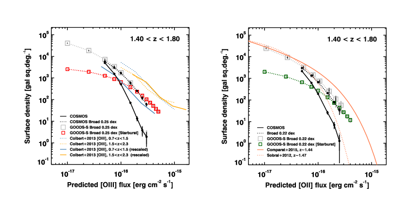
Figure 14: Oxygen line emitters number counts. Left: Cumulative number counts of [O iii] emitters in the redshift range $1.4<z<1.8$. The solid and dotted black lines mark the COSMOS cumulative counts and the upper limits keeping into account the uncertainties on predicted fluxes. Grey squares indicate the upper limit on counts in GOODS-S. Red squares represent the upper limit on counts of simulated starbursting galaxies in GOODS-S. Grey bars indicate the Poissonian $68$% confidence interval. Black bars show the $1\sigma$ uncertainty on cumulative counts from bootstrap and Monte Carlo simulations. Yellow and blue dotted lines show the [O iii] counts from the WISP survey by Colbert et al. 2013. Yellow and blue solid tracks show the same counts, but properly rescaled to match the cosmic volume within $1.4<z<1.8$ and the luminosity distance at $z\sim 1.55$. Right: Cumulative number counts of [O ii] emitters in the redshift range $1.4<z<1.8$. The solid and dotted black lines mark the COSMOS cumulative counts and the upper limits keeping into account the uncertainties on predicted fluxes. Grey squares indicate the upper limits counts in GOODS-S. Green squares represent the upper limit on counts of simulated starbursting galaxies in GOODS-S. Error bars are coded as in the left panel. The orange solid and dotted lines indicate the estimate derived integrating the luminosity functions in Comparat et al. 2015 and Sobral et al. 2012 at $z\sim 1.45$ and assuming their validity over the redshift range $1.4<z<1.8$. Note: The lower and upper (convolved, “broad”) counts can be obtained subtracting and adding the absolute error $\sigma_{\rm conv}$ to the “average” counts in Table 2.

5.3 [OII] and [OIII] number counts at $1.4<z<1.8$

We computed the number counts of oxygen line emitters based on the [O ii] and [O iii] flux predictions in the redshift range $1.4<z<1.8$. We applied the same method described in Section 5.1, keeping into account the uncertainties on the predicted fluxes convolving the number counts with Gaussian curves of fixed width. Results are shown in Figure 14 and reported in Table 2. The [O iii] number counts are roughly consistent with the results from the WISP survey presented in Colbert et al. (2013), once (i) rescaling for the volume and the luminosity distance is properly taken into account, and (ii) low mass galaxies are included in the calculation. Our estimates fall between the WISP counts in the $0.7<z<1.5$ and $1.5<z<2.3$ intervals. Given how we predict [O iii] fluxes (Section 3.3), the increase of the average [O iii]/H$\beta$ ratios and of the MS normalization with redshift can explain the offset between our estimates and Colbert’s et al. (2013). Moreover, low mass galaxies play a critical role, since they have intrinsically higher [O iii]/H$\beta$ ratios. In fact, bright [O iii] emitters in the WISP survey are generally low mass ($M_{\star}\sim 10^{8.5}-10^{9.5}$ $M_{\odot}$, Atek et al. 2011; Henry et al. 2013). The low mass regime is also sensitive to the presence of high sSFR, unobscured, starbursting galaxies, thus we expect them to be relevant for the [O iii] number counts. We simulated their impact on the counts from the GOODS-S sample as detailed in Section 6.3, and we found a substantial extension of counts above $1.5\times 10^{-16}$ erg cm^-2 s^-1, the limit we reach when counting normal Main-Sequence galaxies (Figure 14). Starbursting galaxies are expected to reach [O iii] fluxes of $3\times 10^{-16}$ erg cm^-2 s^-1. In the interval $1.4<z<1.8$, we expect $\sim 1,100$ and $\sim 150$ galaxies deg^-2 above $\geq 1\times 10^{-16}$ and $\geq 2\times 10^{-16}$ erg cm^-2 s^-1, averaging the results for the COSMOS and GOODS-S fields. Including the effect of low-mass starburst, we expect $\sim 1,700$ galaxies deg^-2 for [O iii] fluxes above $\geq 1\times 10^{-16}$.

For what concerns the number counts of [O ii] emitters, the contribution of low mass galaxies and the different mass completeness limits explain the difference between the COSMOS and GOODS-S samples. The number counts we derived fall in the range of recent estimates at $z\sim 1.45$ by Sobral et al. (2012) and Comparat et al. (2015). We derived these counts integrating their LFs assuming their validity over the redshift range $1.4<z<1.8$ and for fluxes up to $3\times 10^{-16}$ erg cm^-2 s^-1, the limit of our estimates. We divided the counts by Comparat et al. (2015) by ln$(10)$ to account for the different normalizations of the two LFs. Our calculations are in agreement with the estimates by Sobral et al. (2012) up to $\sim 1\times 10^{-16}$ erg cm^-2 s^-1, while we find higher counts above this threshold (a factor $2-3.5\times$ at $\sim 2\times 10^{-16}$ erg cm^-2 s^-1 considering our “average” estimate reported in Table 2 for COSMOS and GOODS-S, respectively). On the other hand, we systematically find less counts than in Comparat et al. (2015), a factor $4.5-4\times$ ($3-2.5\times$) at $\sim 1\times 10^{-16}$ erg cm^-2 s^-1 and $11-6.5\times$ ($6-4.5\times$) at $\sim 2\times 10^{-16}$ erg cm^-2 s^-1 considering the “average” estimates (the broadened counts) for COSMOS and GOODS-S, respectively. We note that the LF by Comparat et al. (2015) probes only the tail of the brightest emitters, finding a larger number of them than what extrapolated by a fit at lower fluxes by Sobral et al. (2012) (see Figure 13 in Comparat et al. 2015). Part of the discrepancy we find is due to the correction for the extinction of the Galaxy that Comparat et al. (2015) applied, while we report purely observed and dust reddened fluxes. Moreover, the different sample sizes of Sobral et al. (2012), Comparat et al. (2015), and our work might affect the results in the poorly populated tail of bright emitters. Over the redshift range $1.4<z<1.8$, we expect $2,600$ ($2,700$) and $\sim 400$ ($\sim 500$) galaxies deg^-2 based on the COSMOS (GOODS-S) field “average” estimate for [O ii] fluxes of $\geq 5\times 10^{-17}$ and $\geq 1\times 10^{-16}$ erg cm^-2 s^-1 (Table 2). These fluxes correspond to $\sim 8\sigma$ and $\sim 15\sigma$ detection thresholds expected for the Prime Focus Spectrograph survey in the same redshift range (Takada et al., 2014). When including the effect of low-mass, starbursting galaxies (Section 6.3), we, thus, expect $\sim 3400$ and $\sim 700$ galaxies deg^-2 at fluxes of $\geq 5\times 10^{-17}$ and $\geq 1\times 10^{-16}$ erg cm^-2 s^-1, as derived from the average counts in GOODS-S in the range $1.4<z<1.8$.

6 Discussion

In the previous sections we showed how it is possible to estimate number counts of line emitters using solely the photometric information and a calibration sample of spectroscopically confirmed objects, reaching a precision at least comparable with the one achieved with standard approaches, generally based on small spectroscopic samples and extrapolations of the LFs. We computed the number counts for the redshift slice $1.4<z<1.8$ covered by our calibration sample from the FMOS-COSMOS survey and we extended our calculation for the H$\alpha$ emitters to the $0.9<z<1.8$ interval probed by the Euclid mission, as a reference. We now envisage possible caveats and developments of this work.

6.1 The effect of [N II] lines on low resolution spectroscopy

In Section 5, we computed the galaxy number counts based on the aperture-corrected H$\alpha$ fluxes only. However, future slitless spectroscopy will not be able to resolve the [N ii]-H$\alpha$ complex, resulting in a boost of galaxy number counts when the [N ii] flux is high. In Section 4.1 we found an average line ratio of $\rm{log}($[N ii]/H$\alpha)\sim-0.5$ for the bright emitters observable by Euclid, and we provided a simple parametrization of the relation between log([N ii]/H$\alpha$) and the total observed H$\alpha$ fluxes (Figure 9). This relation can be extended at higher redshift, but it must be taken with caution, being naturally affected by observational biases (Kashino et al., 2017a). We, thus, model the effect of the [N ii] flux boost fitting a first-order polynomial relation to the FMOS-COSMOS observed $\mathrm{log}(M_{\star}/M_{\odot})$ - $\mathrm{log}($[N ii]$/$H$\alpha$$)$ relation (Sample-1, Table 2, Figure 14 in Kashino et al., 2017a) and applying a mass-dependent correction to each source. We show the results on the number counts in Figure 15. We extended the number counts to the $0.9<z<1.8$ interval assuming the same correction. Note that the redshift evolution of the mass-metallicity relation (i.e., Steidel et al., 2014; Sanders et al., 2015) might impact this correction.

We report in Table 3 the counts for H$\alpha$$+$[N ii] emitters. The flux boost due to unresolved [N ii] emission increases by a factor of $\sim 1.8\times$ ($\sim 1.6\times$) the H$\alpha$ number counts above $2\times 10^{-16}$ erg cm^-2 s^-1 in the range $1.4<z<1.8$ ($0.9<z<1.8$), as derived from the average counts both in the COSMOS and GOODS-S fields.

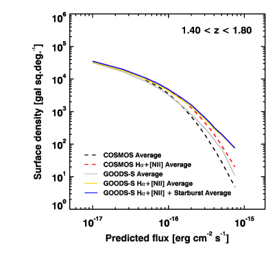
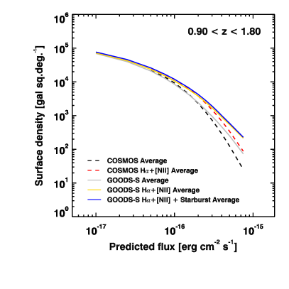
Figure 15: Effect of unresolved [N ii] emission and starbursting galaxies on H$\alpha$ counts. The dashed black and red lines mark the H$\alpha$ and H$\alpha$+[N ii] counts average estimate in the COSMOS field, respectively (Tables 1 and 3). The solid grey and yellow lines mark the H$\alpha$ and H$\alpha$+[N ii] counts in the GOODS-S field. The solid blue line indicates the H$\alpha$+[N ii] counts in the GOODS-S field, including the effect of starbursting galaxies (Table 4). Left: FMOS-COSMOS redshift range of $1.4<z<1.8$. Right: Full redshift range of $0.9<z<1.8$ covered by the forthcoming Euclid mission.

6.2 The AGN contribution

Strong line emitters such as AGN or starbursting galaxies might increase the number counts as well. We flagged and excluded from our COSMOS sample known Chandra detected sources in the catalog by Civano et al. (2016), since we could not reliably predict H$\alpha$ fluxes based on their photometry. However, considering only the Chandra sources with an estimate of the photometric redshift by Salvato et al. (in prep.), $\sim 17$% of the X-ray detected sample by Civano et al. (2016) (671/4016 galaxies) lie at $1.4<z<1.8$, corresponding to 471 objects per deg² in this redshift range. This represents a minimal fraction of the overall population of SFGs composing our COSMOS photometric sample ($31,193$ objects in total). On the other hand, the color-selection we adopted does not prevent low luminosity or obscured AGN to be included in the final sample. Moreover, the FMOS-COSMOS selection function did include some X-ray detected AGN (Silverman et al., 2015). However, only $11$ galaxies in the Chandra catalog by Civano et al. (2016) are detected as H$\alpha$ emitters with fluxes $\geq 2\times 10^{-16}$ erg cm^-2 s^-1, representing a fraction of $8$% of the overall bright FMOS-COSMOS sample. Therefore, X-ray AGN should not provide a significant contribution to the H$\alpha$ number counts at high fluxes in the redshift range $1.4<z<1.8$.

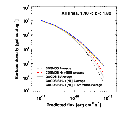
Figure 16: Total cumulative number counts of line emitters at $1.4<z<1.8$. The black dashed line indicates the cumulative number counts obtained adding the average estimates of the H$\alpha$, [O ii], and [O iii] emitter counts in the COSMOS field (Table 1 and 2). The red dashed line shows the counts in COSMOS when taking into account the [N ii] unresolved emission (“average” estimates in Table 3). The grey, gold, and blue solid lines mark the cumulative counts for emitters in GOODS-S considering (i) H$\alpha$, [O ii], and [O iii] emitters; (ii) including the effect of [N ii] unresolved emission as for the COSMOS field; (iii) finally adding the population of low-mass starbursting galaxies (Table 4).

6.3 Starbursting galaxies

Given the large dust attenuation, only few H$\alpha$ photons are expected to escape from massive starbursting galaxies (i.e, lying several times above the main sequence at fixed redshift). However, at moderate stellar masses ($M_{\star}\lesssim 10^{9}-10^{10}$ $M_{\odot}$) galaxies showing high specific SFR (sSFR) and extreme line EWs might contribute to the number counts (Atek et al., 2011). To assess this effect on the cumulative counts of H$\alpha$ emitters, we simulated a population of starbursting galaxies at $M_{\star}<10^{10}$ $M_{\odot}$ artificially increasing their SFRs by a factor of $\times 4$ and considering a volume number density equal to $4$% of the one of main sequence SFGs (Rodighiero et al., 2011). Note that the choice of a mass limit of $10^{10}$ $M_{\odot}$ to simulate starburst is conservative, as extreme sSFR and EW in existing slitless spectroscopic surveys occur at $M_{\star}\sim 10^{8.5}-10^{9.5}$ $M_{\odot}$(Atek et al., 2011). Since more reliable SFRs are available at low stellar masses in GOODS-S than in COSMOS, we used the GOODS-S for the experiment. We, then, recalculated the H$\alpha$ fluxes and the number densities for the starburst population as in Sections 3.1 and 5. We show the results in Figure 15 and report the counts for stabursting galaxies in Table 4. The increase of the H$\alpha$ cumulative number counts due to the low mass, starbursting population is of $\sim 15$% and $20$% at $1\times 10^{-16}$ erg cm^-2 s^-1 and $2\times 10^{-16}$ erg cm^-2 s^-1, respectively, at both $1.4<z<1.8$ and $0.9<z<1.8$. Therefore, our best estimates for H$\alpha$ number counts including the starbursting population are $\sim 3,800$ and $\sim 1,000$ ($\sim 9,700$ and $\sim 2,900$) galaxies deg^-2 in the redshift interval $1.4<z<1.8$ ($0.9<z<1.8$) for H$\alpha$ fluxes $\geq 1\times 10^{-16}$ erg cm^-2 s^-1 and $\geq 2\times 10^{-16}$ erg cm^-2 s^-1, respectively, as evaluated from the average counts in GOODS-S (Tables 1 and 4).

The impact of low-mass starburst on the number counts of [O ii] and [O iii] emitters is relevant (Figure 14, Table 4, and Section 5.3). In the redshift range $1.4<z<1.8$, these galaxies increase by $\sim 50$% the number counts derived from Main-Sequence objects at fluxes $\geq 1\times 10^{-16}$ erg cm^-2 s^-1.

Finally, we underline that, in order to reach their main scientific goals in cosmology, future spectroscopic surveys need to map the highest possible number of spectroscopic redshifts, irrespectively of which lines are detected. We, thus, collected the cumulative number counts of H$\alpha$, [O ii], and [O iii] emitters in the redshift range $1.4<z<1.8$ at which we calibrated the predicted fluxes. The results are shown in Figure 16, where we also included the effect of a possible flux boost due to unresolved [N ii] emission and the impact of starbursting galaxies as detailed above. We did not attempt to extend these predictions to different redshift ranges given the uncertainty of the extrapolations of the recipes we adopted to estimate the oxygen emission lines.

6.4 Estimating a survey effective depth and return

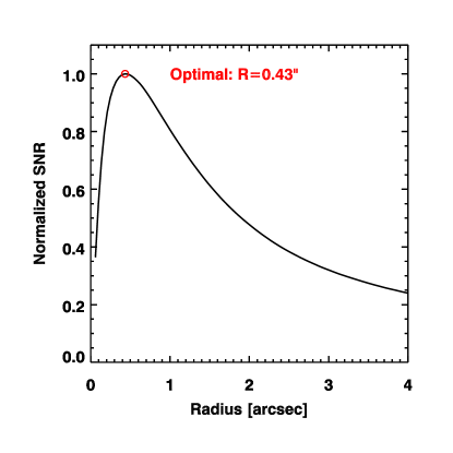
Figure 17: Signal-to-noise ratio in circular aperture photometry of bright H$\alpha$ emitters. The black line represents the signal-to-noise ratio in circular apertures as a function of their radius for the median HST/$i_{814}$ image of bright H$\alpha$ emitters in Figure 11. We normalized the curve to its peak. The red circle marks the radius maximizing the signal-to-noise ratio.

In order to optimize the detectability and, thus, the number of detections for extended objects like galaxies, one has to reach a compromise between (i) recovering as much as possible of galaxies’ flux, which requires large apertures; and (ii) limiting the noise associated with the measurement, obtained minimizing the apertures. This leads to a situation in which the optimal aperture is driven by the galaxy surface brightness profile, as discussed in the previous sections. Moreover, flux measurements are necessarily performed in some apertures, and the ensuing flux losses must be taken into account when analyzing the performances of a survey. For example, spectroscopic surveys with multi-object longslits or fibers with fixed diameters will be affected by losses outside the physically pre-defined apertures. Aperture corrections introduce further uncertainties on the total flux estimates, thus the effective depth of a survey is shallower in terms of total galaxy flux than what computed inside the aperture. A similar effect also influences slitless spectroscopy: despite providing a high-fidelity 2D map of each emission line in galaxies and allowing for recovering the full flux under ideal circumstances, sources must be first robustly identified before emission line fluxes can be measured. The advantage of slitless spectroscopy is that the size and shape of apertures might in principle be adjusted to the size of each object, not being physically limited by a fiber or slit.

Based on the stacked image of the H$\alpha$ emitters with fluxes $\geq 2\times 10^{-16}$ erg cm^-2 s^-1 shown in Figure 11, we estimated the optimal radius for the circular aperture that maximizes its signal-to-noise ratio (Figure 17). This radius is $0.43$” ($\sim 0.9$ $R_{\rm e}$), causing an aperture loss of a factor of $\sim 2.2\times$. The flux losses ensuing any aperture measurement imply a higher “effective” flux limit of a survey – defined as the minimum total emission line flux recoverable above a given signal-to-noise detection threshold – than the “nominal” limit defined in a specific aperture. For example, observations designed to provide secure detections down to a line flux $F_{\rm ap}$ within an aperture of radius $R=R_{\rm e}\sim 0.5"$ (i.e., the “nominal” depth) would set an “effective” depth of $F_{\rm eff}=2F_{\rm ap}$. This effective depth can be used to assess the “return” of the survey, i.e., the number of recoverable spectroscopic redshifts, by comparing with the cumulative number counts of galaxies above $F_{\rm eff}$ as in Figures 12 and 14, and Tables 1 and 2. In fact, as common practice, we derived the line fluxes in Section 3 from integrated, observed SED properties, thus not taking into account the size of the galaxies. If neglected, aperture losses cause an increase of the effective flux limit with respect to the nominal one and a decrease of the return at any flux. However, given the shape of the number counts, this effect is more pronounced at high than at low fluxes. For reference, the total number of detections for a nominal sensitivity $F_{\rm ap}\geq 2\times 10^{-16}$ erg cm^-2 s^-1 inside a 0.5” circular aperture would correspond to a decrease by a factor of $\sim 10$ of the return when considering the effective depth $F_{\rm eff}=2F_{\rm ap}\geq 4\times 10^{-16}$, considering the case of H$\alpha$ emitters in the COSMOS field (Table 1). On the other hand, for $F_{\rm ap}\geq 5\times 10^{-17}$ erg cm^-2 s^-1, the return drops by a factor of $\sim 3$ when estimating it at the corresponding effective depth $F_{\rm eff}\geq 1\times 10^{-16}$ erg cm^-2 s^-1. The smaller factor at lower fluxes is due to the flattening of the counts and it could be overestimated, since such weaker emitters likely have typical sizes smaller than we estimated in Section 4.3, resulting in lower flux losses. Note that, when computing counts within fixed apertures, we kept into account the evolution of the intrinsic sizes of SFGs ($R_{\rm e}\propto(1+z)^{-0.8}$, van der Wel et al. 2014; Straatman et al. 2015) when assessing the effect for redshift intervals larger than $1.4<z<1.8$. Moreover, the effect of the PSF of HST/ACS is negligible on the estimate of the optimal aperture, while it may play a role for ground based and seeing-limited observations.

Adopting apertures larger than the optimal one, the flux losses and the difference between nominal and effective depths are reduced. For example, considering circular apertures of $2"$ diameter or, equivalently, rectangular apertures of $1"\times 3.4"$ ($\sim 2R_{\rm e}\times 7R_{\rm e}$) would reduce the aperture losses to only a factor of $\sim 1.2$, the pseudo-slit mimicking the longslit spectroscopic case and a possible choice for the extraction of slitless spectra. In this case, the effective depth would be only $1.2\times$ shallower than the nominal depth, and the implied change in return would also be fairly limited (a factor of $1.2-1.6$ at $5\times 10^{-17}$ and $2\times 10^{-16}$ erg cm^-2 s^-1, respectively), if aperture losses are neglected. Note, however, that at fixed integration time, using apertures of any shape, but larger - or smaller - than the optimal one decreases the achievable nominal signal-to-noise ratio, further reducing the return with respect to the optimal case presented above. Doubling the aperture area does not come for free, as it requires a $4\times$ higher integration time to reach the same flux limit with the same signal-to-noise ratio. Hence, adopting larger apertures for line detection to reduce aperture losses, without adjusting accordingly the exposure time, is not a way to boost the return of a survey, as it instead reduces the return with respect to the optimal case. Following the definitions of “effective” and “nominal” depths, any possible combination of flux losses and corresponding survey returns can be estimated using the profile given in Figure 11 and the cumulative number counts for total fluxes in Figure 12, 14, 15, and 16 and Tables 1-4, according to the specific apertures set in each survey. We emphasize that the optimal aperture suggested here ($R\sim 0.5^{\prime\prime}$) is rather large by space standards, corresponding to $\sim 5\times$ the full width half maximum of HST/ACS point spread function.

We warn the reader that several other effects might reduce the possible impact of these findings. First, our sizes are not directly measured on H$\alpha$ emission line maps, but based on the UV rest-frame proxy, and it is perhaps a surprising finding that aperture losses are so large even with a $R\sim 0.5"$ aperture on images with the typical HST spatial resolution. We cannot rule out that individual bright emitters might be more compact than the median we show in Figure 11, although the attenuation of UV continuum light is expected to be fully comparable to that of H$\alpha$, and both are tracing SFRs. Then, for low spectral resolution observations, line blending (i.e., [N ii]+H$\alpha$) will boost the number counts. On the other hand, resolving the emission lines, as it might be expected for longslit or fiber spectroscopy from the ground, would cause the opposite effect, reducing the signal-to-noise per resolution element. Finally, AGN and starbursting galaxies can further increase the number counts in the brightest tail, considering their expected compact emission and high EW. We caution the reader that this is a simple experiment based on a specific class of bright H$\alpha$ emitters, with an average radially symmetric shape, a disk-like light profile, and a typical HST/ACS point spread function. The effect of seeing and the exact PSF shape of each set of observations can be modeled convolving the profile in Figure 11, assessing its effect on the optimal aperture. Future simulations might address several open issues with detailed descriptions of the specific characteristics of each survey, which is beyond the scope of this work.

7 Conclusions

We have shown that fluxes of rest-frame optical emission lines can be reliably estimated for thousands of galaxies on the basis of good quality multicolor photometry. We have further explored one of the possible applications of having this information for large samples of galaxies, namely to establish number counts and to investigate the observable and physical properties of line emitters that will be observed by cosmological surveys. In particular:

• We accurately predicted H$\alpha$ fluxes for a sample of color-selected SFGs in COSMOS and GOODS-S at redshift $1.4<z<1.8$ based on their SFRs and dust attenuation estimates from SED modeling. These galaxies fairly represent the normal main sequence population at this redshift. We calibrated the predicted fluxes against spectroscopic observations from the FMOS-COSMOS survey. The statistical uncertainty on the final predicted fluxes is $\sigma_{\rm Pred}\sim 0.1-0.2$ dex (Figure 3).

• We predicted the fluxes of the H$\beta$, [O ii], and [O iii] lines applying simple empirical recipes and calibrating with spectroscopically confirmed galaxies from the FMOS-COSMOS survey and data publicly available.

• We computed the cumulative number counts of H$\alpha$ emitters in the redshift range $1.4<z<1.8$, finding a broad agreement with existing data in literature and the empirical curves by Pozzetti et al. (2016) modeling the evolution of the H$\alpha$ luminosity function with redshift (Figure 12). We obtain fully consistent results when we properly take into account the uncertainty on the predicted H$\alpha$ fluxes, effectively enhancing the number counts at large fluxes.

• We extended the H$\alpha$ number counts to the redshift range $0.9<z<1.8$ covered by future surveys such as Euclid and WFIRST. We adopted a physically motivated approach, modeling the evolution of the main sequence of galaxies with redshift and including the effect of the luminosity distance on the observed fluxes. This method provides results consistent with models and datasets in literature, while returning $\sim 1.5\times$ higher counts for fluxes up to $\geq 2\times 10^{-16}$ erg cm^-2 s^-1 than a simple volume rescaling.

• We argue that the evolution of the MS of galaxies is enough to reproduce the time evolution of the differential number counts $dN/dz$ in the range $0.2<z<2.5$, in good agreement with the current data (Figure 13).

• We computed the number counts for [O ii] and [O iii] emitters in the redshift range $1.4<z<1.8$, extending the predictions to lower fluxes (Figure 14). Our estimates of [O iii] counts are in agreement with previous works once the effect of low-mass galaxies is taken into account. On the other hand, we revise towards lower values the tail of the brightest [O ii] emitters at high redshift.

• We investigated the properties of the typical H$\alpha$ emitters visibile in future wide spectroscopic surveys with observed H$\alpha$ fluxes $\geq 2\times 10^{-16}$ erg cm^-2 s^-1. We find them massive ($\rm{log}(M_{\star}/M_{\odot})\rangle=10.7\pm 0.4$), luminous in observed optical and near-IR bands, and with extended UV sizes ($R_{\rm e}\sim 0.48"=4.4$ kpc at $z\sim 1.5$). We estimate average [N ii]/H$\alpha$ ratio and rest-frame EW(H$\alpha$) of log([N ii]/H$\alpha$)$=-0.52\pm 0.01$ and log[EW(H$\alpha$)]$=2.05\pm 0.01$, respectively.

• We examine caveats and possible extensions of this work, including potential counts boosting or decrease by several factors. Failing at resolving the [N ii] emission or the inclusion of AGN and low mass, unobscured, starbursting galaxies with large sSFR and EW might enhance the counts of bright emitters. The impact of low-mass, high-sSFR galaxies is particularly strong on the number counts of oxygen emitters ($\sim 50$% increase for fluxes $\geq 1\times 10^{-16}$ erg cm^-2 s^-1).

• We further discuss the possible optimization of sources detection and explore the relation between the “nominal” and “effective” depths of a set of observations. We show how the latter is relevant to estimate the “return” of a survey in terms of recoverable spectroscopic redshifts. We find that an “optimal” circular aperture of $R\sim 0.5$” maximizes the signal-to-noise, causing a factor of $\sim 2\times$ flux losses that can correspond to a drop of the return, if neglected.

• We release a catalog containing all the relevant photometric properties and the line fluxes used in this work.

Table 1: Cumulative number counts of H$\alpha$ emitters from the COSMOS and GOODS-S photometric samples.

Flux limit

COSMOS

GOODS-S

[$10^{-16}$ erg cm-2 s-1]

$1.4<z<1.8$

$0.9<z<1.8$

$1.4<z<1.8$

$0.9<z<1.8$

Averagea

$\sigma_{\rm conv}$b

$\sigma_{\rm P,68}$c

$\sigma_{\rm MC}$d

Average

$\sigma_{\rm conv}$

$\sigma_{\rm P,68}$

$\sigma_{\rm MC}$

Average

$\sigma_{\rm conv}$

$\sigma_{\rm P,68}$

$\sigma_{\rm MC}$

Average

$\sigma_{\rm conv}$

$\sigma_{\rm P,68}$

$\sigma_{\rm MC}$

[deg-2]

[deg-2]

[deg-2]

[deg-2]

[deg-2]

[deg-2]

[deg-2]

[deg-2]

[deg-2]

[deg-2]

[deg-2]

[deg-2]

[deg-2]

[deg-2]

[deg-2]

[deg-2]

$\geq 0.10$

–

–

–

–

–

–

–

–

$31635$

$\pm 195$

$\pm 776$

$\pm 2485$

$69400$

$\pm 449$

$\pm 1140$

$\pm 5053$

$\geq 0.25$

–

–

–

–

–

–

–

–

$16936$

$\pm 99$

$\pm 573$

$\pm 2024$

$39661$

$\pm 18$

$\pm 869$

$\pm 4239$

$\geq 0.50$

$9318$

$\pm 78$

$\pm 78$

$\pm 250$

$21422$

$\pm 357$

$\pm 118$

$\pm 576$

$8467$

$\pm 344$

$\pm 404$

$\pm 1207$

$20999$

$\pm 582$

$\pm 629$

$\pm 2776$

$\geq 0.75$

$5671$

$\pm 231$

$\pm 59$

$\pm 132$

$13994$

$\pm 310$

$\pm 93$

$\pm 342$

$5107$

$\pm 270$

$\pm 316$

$\pm 675$

$12809$

$\pm 745$

$\pm 488$

$\pm 1709$

$\geq 1.0$

$3555$

$\pm 324$

$\pm 46$

$\pm 86$

$9328$

$\pm 594$

$\pm 75$

$\pm 216$

$3225$

$\pm 326$

$\pm 249$

$\pm 425$

$8487$

$\pm 702$

$\pm 396$

$\pm 1094$

$\geq 1.5$

$1490$

$\pm 327$

$\pm 28$

$\pm 50$

$4468$

$\pm 643$

$\pm 50$

$\pm 118$

$1524$

$\pm 250$

$\pm 172$

$\pm 216$

$4283$

$\pm 552$

$\pm 280$

$\pm 554$

$\geq 2.0$

$706$

$\pm 228$

$\pm 18$

$\pm 26$

$2301$

$\pm 545$

$\pm 34$

$\pm 68$

$823$

$\pm 177$

$\pm 128$

$\pm 104$

$2421$

$\pm 429$

$\pm 210$

$\pm 296$

$\geq 2.5$

$364$

$\pm 152$

$\pm 12$

$\pm 15$

$1262$

$\pm 419$

$\pm 24$

$\pm 40$

$481$

$\pm 131$

$\pm 100$

$\pm 63$

$1471$

$\pm 337$

$\pm 163$

$\pm 165$

$\geq 3.0$

$199$

$\pm 102$

$\pm 8$

$\pm 10$

$737$

$\pm 304$

$\pm 17$

$\pm 24$

$309$

$\pm 88$

$\pm 84$

$\pm 38$

$958$

$\pm 253$

$\pm 133$

$\pm 100$

$\geq 3.5$

$114$

$\pm 70$

$\pm 6$

$\pm 7$

$449$

$\pm 219$

$\pm 13$

$\pm 16$

$208$

$\pm 60$

$\pm 72$

$\pm 25$

$655$

$\pm 190$

$\pm 112$

$\pm 64$

$\geq 4.0$

$69$

$\pm 47$

$\pm 4$

$\pm 4$

$284$

$\pm 159$

$\pm 10$

$\pm 11$

$140$

$\pm 47$

$\pm 62$

$\pm 18$

$460$

$\pm 148$

$\pm 95$

$\pm 43$

$\geq 4.5$

$44$

$\pm 32$

$\pm 3$

$\pm 3$

$187$

$\pm 114$

$\pm 7$

$\pm 8$

$94$

$\pm 39$

$\pm 54$

$\pm 13$

$336$

$\pm 114$

$\pm 84$

$\pm 32$

$\geq 5.0$

$29$

$\pm 22$

$\pm 3$

$\pm 2$

$126$

$\pm 84$

$\pm 6$

$\pm 6$

$76$

$\pm 20$

$\pm 54$

$\pm 8$

$254$

$\pm 87$

$\pm 76$

$\pm 25$

$\geq 7.5$

$5$

$\pm 4$

$\pm 1$

$\pm 1$

$25$

$\pm 19$

$\pm 3$

$\pm 2$

$11$

$\pm 11$

–

–

$73$

$\pm 34$

$\pm 27$

$\pm 5$

• Mean of the convolved and unconvolved number counts (Section 5.1). Note: The lower and upper (convolved, “broad”) counts shown in Figure 12 can be obtained subtracting and adding the absolute error $\sigma_{\rm conv}$ to the counts reported in this column.

• Absolute error associated with the convolution of the lower counts with a Gaussian curve $0.19$ dex wide ($\rm{[convolved\,counts-unconvolved\,counts]/2}$, Section 5.1).

• Poissonian $68$% confidence interval of the unconvolved counts. The naturally asymmetric Poissonian uncertainties have been round up to the highest value between the lower and upper limits.

• Monte Carlo bootstrap uncertainties on the unconvolved counts.

Table 2: Cumulative number counts of [O ii] and [O iii] emitters from the COSMOS and GOODS-S photometric samples in the redshift range $1.4<z<1.8$.

Flux limit

COSMOS

GOODS-S

[$10^{-16}$ erg cm-2 s-1]

[O ii]$\lambda\,3727$ Å

[O iii]$\lambda\,5007$ Å

[O ii]$\lambda\,3727$ Å

[O iii]$\lambda\,5007$ Å

Averagea

$\sigma_{\rm conv}$b

$\sigma_{\rm P,68}$c

$\sigma_{\rm MC}$d

Average

$\sigma_{\rm conv}$

$\sigma_{\rm P,68}$

$\sigma_{\rm MC}$

Average

$\sigma_{\rm conv}$

$\sigma_{\rm P,68}$

$\sigma_{\rm MC}$

Average

$\sigma_{\rm conv}$

$\sigma_{\rm P,68}$

$\sigma_{\rm MC}$

[deg-2]

[deg-2]

[deg-2]

[deg-2]

[deg-2]

[deg-2]

[deg-2]

[deg-2]

[deg-2]

[deg-2]

[deg-2]

[deg-2]

[deg-2]

[deg-2]

[deg-2]

[deg-2]

$\geq 0.10$

–

–

–

–

–

–

–

–

$23727$

$\pm 317$

$\pm 672$

$\pm 2016$

$41401$

$\pm 968$

$\pm 898$

$\pm 2415$

$\geq 0.25$

–

–

–

–

–

–

–

–

$8705$

$\pm 527$

$\pm 405$

$\pm 1071$

$17874$

$\pm 668$

$\pm 579$

$\pm 1653$

$\geq 0.50$

$2573$

$\pm 426$

$\pm 37$

$\pm 77$

$5342$

$\pm 388$

$\pm 57$

$\pm 129$

$2729$

$\pm 495$

$\pm 221$

$\pm 386$

$6084$

$\pm 1062$

$\pm 322$

$\pm 676$

$\geq 0.75$

$981$

$\pm 362$

$\pm 20$

$\pm 28$

$2272$

$\pm 711$

$\pm 32$

$\pm 40$

$1093$

$\pm 354$

$\pm 135$

$\pm 137$

$2385$

$\pm 963$

$\pm 180$

$\pm 271$

$\geq 1.0$

$431$

$\pm 239$

$\pm 12$

$\pm 16$

$1083$

$\pm 574$

$\pm 19$

$\pm 25$

$482$

$\pm 261$

$\pm 84$

$\pm 74$

$1079$

$\pm 673$

$\pm 106$

$\pm 133$

$\geq 1.5$

$116$

$\pm 90$

$\pm 5$

$\pm 5$

$334$

$\pm 262$

$\pm 7$

$\pm 9$

$163$

$\pm 90$

$\pm 58$

$\pm 22$

$332$

$\pm 259$

$\pm 58$

$\pm 41$

$\geq 2.0$

$42$

$\pm 35$

$\pm 3$

$\pm 2$

$132$

$\pm 118$

$\pm 4$

$\pm 3$

$73$

$\pm 37$

$\pm 48$

$\pm 9$

–

–

–

–

$\geq 2.5$

$17$

$\pm 16$

$\pm 2$

$\pm 1$

$60$

$\pm 57$

$\pm 2$

$\pm 2$

$38$

$\pm 19$

$\pm 42$

$\pm 1$

–

–

–

–

$\geq 3.0$

–

–

–

–

$31$

$\pm 29$

$\pm 2$

$\pm 1$

–

–

–

–

–

–

–

–

• Mean of the convolved and unconvolved number counts (Section 5.1). Note: The lower and upper (convolved, “broad”) counts shown in Figure 14 can be obtained subtracting and adding the absolute error $\sigma_{\rm conv}$ to the counts reported in this column.

• Absolute error associated with the convolution of the lower counts with Gaussian curves $0.22$ dex and $0.25$ dex wide for [O ii] and [O iii], respectively ($\rm{[convolved\,counts-unconvolved\,counts]/2}$, Section 5.1).

• Poissonian $68$% confidence interval of the lower counts. The naturally asymmetric Poissonian uncertainties have been round up to the highest value between the lower and upper limits.

• Monte Carlo bootstrap uncertainties on the lower counts.

Table 3: Cumulative number counts of H$\alpha$$+$[N ii] emitters from the COSMOS and GOODS-S photometric samples.

Flux limit

COSMOS

GOODS-S

[$10^{-16}$ erg cm-2 s-1]

$1.4<z<1.8$

$0.9<z<1.8$

$1.4<z<1.8$

$0.9<z<1.8$

H$\alpha$+[N ii]a

$\sigma_{\rm conv}$b

$\sigma_{\rm P,68}$c

H$\alpha$+[N ii]

$\sigma_{\rm conv}$

$\sigma_{\rm P,68}$

H$\alpha$+[N ii]

$\sigma_{\rm conv}$

$\sigma_{\rm P,68}$

H$\alpha$+[N ii]

$\sigma_{\rm conv}$

$\sigma_{\rm P,68}$

[deg-2]

[deg-2]

[deg-2]

[deg-2]

[deg-2]

[deg-2]

[deg-2]

[deg-2]

[deg-2]

[deg-2]

[deg-2]

[deg-2]

$\geq 0.10$

–

–

–

–

–

–

$33024$

$\pm 144$

$\pm 793$

$72042$

$\pm 397$

$\pm 1162$

$\geq 0.25$

–

–

–

–

–

–

$18304$

$\pm 120$

$\pm 595$

$42435$

$\pm 30$

$\pm 898$

$\geq 0.50$

$10568$

$\pm 122$

$\pm 83$

$23705$

$\pm 408$

$\pm 124$

$9767$

$\pm 333$

$\pm 434$

$23649$

$\pm 571$

$\pm 668$

$\geq 0.75$

$7019$

$\pm 157$

$\pm 66$

$16620$

$\pm 171$

$\pm 102$

$6276$

$\pm 257$

$\pm 350$

$15250$

$\pm 715$

$\pm 534$

$\geq 1.0$

$4813$

$\pm 250$

$\pm 54$

$11904$

$\pm 441$

$\pm 86$

$4271$

$\pm 301$

$\pm 288$

$10700$

$\pm 660$

$\pm 447$

$\geq 1.5$

$2408$

$\pm 304$

$\pm 37$

$6530$

$\pm 563$

$\pm 62$

$2300$

$\pm 251$

$\pm 212$

$6027$

$\pm 530$

$\pm 336$

$\geq 2.0$

$1308$

$\pm 262$

$\pm 26$

$3796$

$\pm 559$

$\pm 46$

$1428$

$\pm 154$

$\pm 172$

$3789$

$\pm 406$

$\pm 267$

$\geq 2.5$

$762$

$\pm 204$

$\pm 19$

$2320$

$\pm 491$

$\pm 35$

$875$

$\pm 173$

$\pm 133$

$2490$

$\pm 366$

$\pm 216$

$\geq 3.0$

$468$

$\pm 154$

$\pm 15$

$1488$

$\pm 398$

$\pm 27$

$595$

$\pm 133$

$\pm 111$

$1717$

$\pm 313$

$\pm 179$

$\geq 3.5$

$301$

$\pm 114$

$\pm 11$

$992$

$\pm 315$

$\pm 21$

$419$

$\pm 106$

$\pm 96$

$1224$

$\pm 268$

$\pm 151$

$\geq 4.0$

$198$

$\pm 88$

$\pm 9$

$680$

$\pm 249$

$\pm 17$

$297$

$\pm 94$

$\pm 81$

$898$

$\pm 230$

$\pm 130$

$\geq 4.5$

$136$

$\pm 65$

$\pm 7$

$480$

$\pm 196$

$\pm 14$

$233$

$\pm 67$

$\pm 75$

$690$

$\pm 182$

$\pm 116$

$\geq 5.0$

$93$

$\pm 52$

$\pm 6$

$346$

$\pm 155$

$\pm 12$

$191$

$\pm 44$

$\pm 72$

$547$

$\pm 142$

$\pm 106$

$\geq 7.5$

$20$

$\pm 15$

$\pm 3$

$88$

$\pm 52$

$\pm 5$

$73$

$\pm 18$

$\pm 32$

$215$

$\pm 54$

$\pm 55$

• Mean of the convolved and unconvolved number counts of H$\alpha$+[N ii] emitters (Section 6.1).

• Absolute error associated with the convolution of the lower counts with a Gaussian curve $0.19$ dex wide ($\rm{[convolved\,counts-unconvolved\,counts]/2}$, Section 5.1).

• Poissonian $68$% confidence interval of the lower counts. The naturally asymmetric Poissonian uncertainties have been round up to the highest value between the lower and upper limits.

Table 4: Cumulative number counts of starbursting emitters from the GOODS-S photometric sample.

Flux limit

GOODS-S Starburst

[$10^{-16}$ erg cm-2 s-1]

$1.4<z<1.8$

$0.9<z<1.8$

H$\alpha$a

$\sigma_{\rm conv}$b

$\sigma_{\rm P,68}$c

[O ii]d

$\sigma_{\rm conv}$e

$\sigma_{\rm P,68}$

[O iii]f

$\sigma_{\rm conv}$g

$\sigma_{\rm P,68}$

H$\alpha$

$\sigma_{\rm conv}$

$\sigma_{\rm P,68}$

[deg-2]

[deg-2]

[deg-2]

[deg-2]

[deg-2]

[deg-2]

[deg-2]

[deg-2]

[deg-2]

[deg-2]

[deg-2]

[deg-2]

$\geq 0.10$

$2273$

$\pm 18$

$\pm 42$

$2040$

$\pm 30$

$\pm 40$

$2606$

$\pm 59$

$\pm 45$

$4758$

$\pm 40$

$\pm 60$

$\geq 0.25$

$1592$

$\pm 14$

$\pm 35$

$1212$

$\pm 3$

$\pm 31$

$1968$

$\pm 48$

$\pm 39$

$3469$

$\pm 35$

$\pm 51$

$\geq 0.50$

$1025$

$\pm 5$

$\pm 28$

$636$

$\pm 23$

$\pm 22$

$1271$

$\pm 2$

$\pm 31$

$2324$

$\pm 1$

$\pm 42$

$\geq 0.75$

$718$

$\pm 13$

$\pm 23$

$379$

$\pm 28$

$\pm 17$

$861$

$\pm 29$

$\pm 25$

$1667$

$\pm 28$

$\pm 35$

$\geq 1.0$

$529$

$\pm 12$

$\pm 20$

$236$

$\pm 34$

$\pm 13$

$602$

$\pm 47$

$\pm 21$

$1256$

$\pm 31$

$\pm 31$

$\geq 1.5$

$294$

$\pm 24$

$\pm 15$

$107$

$\pm 26$

$\pm 8$

$327$

$\pm 48$

$\pm 15$

$756$

$\pm 40$

$\pm 24$

$\geq 2.0$

$177$

$\pm 22$

$\pm 11$

$55$

$\pm 19$

$\pm 6$

$184$

$\pm 48$

$\pm 11$

$476$

$\pm 45$

$\pm 18$

$\geq 2.5$

$109$

$\pm 20$

$\pm 9$

$30$

$\pm 14$

$\pm 4$

$110$

$\pm 42$

$\pm 8$

$311$

$\pm 44$

$\pm 15$

$\geq 3.0$

$71$

$\pm 16$

$\pm 7$

$18$

$\pm 9$

$\pm 3$

$70$

$\pm 33$

$\pm 6$

$210$

$\pm 39$

$\pm 12$

$\geq 3.5$

$44$

$\pm 16$

$\pm 5$

$11$

$\pm 7$

$\pm 2$

$44$

$\pm 27$

$\pm 4$

$142$

$\pm 36$

$\pm 10$

$\geq 4.0$

$28$

$\pm 14$

$\pm 4$

$6$

$\pm 6$

$\pm 2$

$31$

$\pm 20$

$\pm 4$

$98$

$\pm 32$

$\pm 8$

$\geq 4.5$

$19$

$\pm 11$

$\pm 3$

–

–

–

$21$

$\pm 17$

$\pm 2$

$70$

$\pm 27$

$\pm 6$

$\geq 5.0$

$14$

$\pm 8$

$\pm 3$

–

–

–

$15$

$\pm 13$

$\pm 2$

$51$

$\pm 22$

$\pm 5$

$\geq 7.5$

$3$

$\pm 2$

$\pm 1$

–

–

–

–

–

–

$13$

$\pm 8$

$\pm 2$

• Mean of the convolved and unconvolved number counts of H$\alpha$ starbursting emitters (Section 6.3).

• Absolute error associated with the convolution of the H$\alpha$ unconvolved counts with a Gaussian curve $0.19$ dex wide ($\rm{[convolved\,counts-unconvolved\,counts]/2}$, Section 5.1).

• Poissonian $68$% confidence interval of the lower counts. The naturally asymmetric Poissonian uncertainties have been round up to the highest value between the lower and upper limits.

• Mean of the convolved and unconvolved number counts of [O ii] starbursting emitters.

• Absolute error associated with the convolution of the [O ii] lower counts with a Gaussian curve $0.22$ dex wide.

• Mean of the convolved and unconvolved number counts of [O iii] starbursting emitters.

• Absolute error associated with the convolution of the [O iii] lower counts with a Gaussian curve $0.25$ dex wide.

Appendix A Individual bright H$\alpha$ emitters

We show in Figure 18 a random selection of H$\alpha$ emitters with predicted H$\alpha$ fluxes $\geq 2\times 10^{-16}$ erg cm^-2 s^-1. The images are in the HST/$i_{814}$ band.

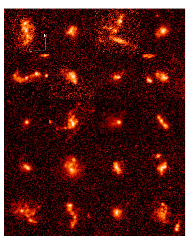
Figure 18: HST/$i_{814}$ cutouts of bright H$\alpha$ emitters in COSMOS. The cutouts show a random sample of emitters with predicted H$\alpha$ fluxes $\geq 2\times 10^{-16}$ erg cm^-2 s^-1 at $1.4<z<1.8$. The size is $3.75"\times 3.75"$. The images are aligned North-East and they are scaled to the same background level. The white bar shown in the top-left panel is 1” long.

Appendix B Catalog of line fluxes predictions

Table 5: Catalog of relevant SED-derived quantities and emission line flux predictions for the COSMOS sample (a machine-readable version is available online).

IDa	RA	DEC	log${}_{10}(M_{\star})$	log${}_{10}(\rm{SFR})$	$z_{\rm phot}$	$A_{\rm V}$	H$\alpha$	[O ii]	[O iii]	H$\beta$	$f_{\rm H\beta}$b
	[deg]	[deg]	[$M_{\odot}$]	[$M_{\odot}$ yr-1]		[mag]	[$10^{-16}$ erg cm-2 s-1]	[$10^{-16}$ erg cm-2 s-1]	[$10^{-16}$ erg cm-2 s-1]	[$10^{-16}$ erg cm-2 s-1]
219860	150.322350	1.61483180	9.69	0.92	1.64	0.70	0.29	0.16	0.27	0.08	1.00
219985	149.984920	1.61497840	9.46	0.58	1.62	0.20	0.23	0.19	0.31	0.07	1.00
220037	149.890400	1.61494710	9.63	0.94	1.63	0.70	0.31	0.17	0.30	0.08	1.00
220136	150.353750	1.61500880	10.45	1.88	1.60	2.00	0.76	0.13	0.19	0.11	1.15
220152	149.759090	1.61519360	9.67	0.78	1.51	0.80	0.24	0.12	0.22	0.06	1.00
…	…	…	…	…	…	…	…	…	…	…	…

• Galaxy ID from (Laigle et al., 2016).

• Stellar absorption correction factor (Section 3.2).

Table 6: Catalog of relevant SED-derived quantities and emission line flux predictions for the GOODS-S sample (a machine-readable version is available online).

ID	RA	DEC	log${}_{10}(M_{\star})$	log${}_{10}(\rm{SFR})$	$z_{\rm phot}$	$A_{\rm V}$	H$\alpha$	[O ii]	[O iii]	H$\beta$	$f_{\rm H\beta}$a
	[deg]	[deg]	[$M_{\odot}$]	[$M_{\odot}$ yr-1]		[mag]	[$10^{-16}$ erg cm-2 s-1]	[$10^{-16}$ erg cm-2 s-1]	[$10^{-16}$ erg cm-2 s-1]	[$10^{-16}$ erg cm-2 s-1]
1	53.08488800	-27.95581300	9.51	1.40	1.59	1.00	0.71	0.29	0.66	0.16	1.00
2	53.09927000	-27.95315400	9.51	0.55	1.70	0.40	0.15	0.11	0.19	0.05	1.00
3	53.07999000	-27.95205100	10.13	1.02	1.47	1.60	0.20	0.05	0.08	0.03	1.06
4	53.10614800	-27.95160700	9.34	0.96	1.66	0.20	0.52	0.43	0.76	0.17	1.00
5	53.10593400	-27.95165800	9.54	1.14	1.73	0.40	0.58	0.40	0.69	0.17	1.00
6	53.09929700	-27.94932000	8.74	0.17	1.55	0.60	0.07	0.04	0.11	0.02	1.00
…	…	…	…	…	…	…	…	…	…	…	…

• Stellar absorption correction factor (Section 3.2).

References

- Abazajian et al. (2009) Abazajian K. N., et al., 2009, ApJS, 182, 543
- Arnouts et al. (2013) Arnouts S., et al., 2013, A&A, 558, A67
- Atek et al. (2011) Atek H., et al., 2011, ApJ, 743, 121
- Bertin & Arnouts (1996) Bertin E., Arnouts S., 1996, A&AS, 117, 393
- Blake et al. (2011) Blake C., et al., 2011, MNRAS, 418, 1707
- Bolzonella et al. (2000) Bolzonella M., Miralles J.-M., Pelló R., 2000, A&A, 363, 476
- Bruzual & Charlot (2003) Bruzual G., Charlot S., 2003, MNRAS, 344, 1000
- Calzetti et al. (2000) Calzetti D., Armus L., Bohlin R. C., Kinney A. L., Koornneef J., Storchi-Bergmann T., 2000, ApJ, 533, 682
- Cardelli et al. (1989) Cardelli J. A., Clayton G. C., Mathis J. S., 1989, ApJ, 345, 245
- Chabrier (2003) Chabrier G., 2003, PASP, 115, 763
- Cirasuolo et al. (2014) Cirasuolo M., et al., 2014, in Ground-based and Airborne Instrumentation for Astronomy V. p. 91470N, doi:10.1117/12.2056012
- Civano et al. (2016) Civano F., et al., 2016, ApJ, 819, 62
- Colbert et al. (2013) Colbert J. W., et al., 2013, ApJ, 779, 34
- Comparat et al. (2015) Comparat J., et al., 2015, A&A, 575, A40
- Cullen et al. (2016) Cullen F., Cirasuolo M., Kewley L. J., McLure R. J., Dunlop J. S., Bowler R. A. A., 2016, MNRAS, 460, 3002
- Daddi et al. (2007) Daddi E., et al., 2007, ApJ, 670, 156
- Dawson et al. (2013) Dawson K. S., et al., 2013, AJ, 145, 10
- Fitzpatrick (1999) Fitzpatrick E. L., 1999, PASP, 111, 63
- Fumagalli et al. (2012) Fumagalli M., et al., 2012, ApJ, 757, L22
- Geach et al. (2010) Geach J. E., et al., 2010, MNRAS, 402, 1330
- Green et al. (2012) Green J., et al., 2012, preprint, (arXiv:1208.4012)
- Henry et al. (2013) Henry A., et al., 2013, ApJ, 776, L27
- Ilbert et al. (2006) Ilbert O., et al., 2006, A&A, 457, 841
- Ilbert et al. (2013) Ilbert O., et al., 2013, A&A, 556, A55
- Jouvel et al. (2009) Jouvel S., et al., 2009, A&A, 504, 359
- Juneau et al. (2011) Juneau S., Dickinson M., Alexander D. M., Salim S., 2011, ApJ, 736, 104
- Juneau et al. (2014) Juneau S., et al., 2014, ApJ, 788, 88
- Kaasinen et al. (2017) Kaasinen M., Bian F., Groves B., Kewley L. J., Gupta A., 2017, MNRAS, 465, 3220
- Kashino et al. (2013) Kashino D., et al., 2013, ApJ, 777, L8
- Kashino et al. (2017a) Kashino D., et al., 2017a, ApJ, 835, 88
- Kashino et al. (2017b) Kashino D., et al., 2017b, ApJ, 843, 138
- Kennicutt (1998) Kennicutt Jr. R. C., 1998, ARA&A, 36, 189
- Kewley et al. (2004) Kewley L. J., Geller M. J., Jansen R. A., 2004, AJ, 127, 2002
- Kewley et al. (2013) Kewley L. J., Dopita M. A., Leitherer C., Davé R., Yuan T., Allen M., Groves B., Sutherland R., 2013, ApJ, 774, 100
- Kimura et al. (2010) Kimura M., et al., 2010, PASJ, 62, 1135
- Laigle et al. (2016) Laigle C., et al., 2016, ApJS, 224, 24
- Laureijs (2009) Laureijs R., 2009, preprint, (arXiv:0912.0914)
- Levi et al. (2013) Levi M., et al., 2013, preprint, (arXiv:1308.0847)
- Lilly et al. (2007) Lilly S. J., et al., 2007, ApJS, 172, 70
- Mármol-Queraltó et al. (2016) Mármol-Queraltó E., McLure R. J., Cullen F., Dunlop J. S., Fontana A., McLeod D. J., 2016, MNRAS, 460, 3587
- Mehta et al. (2015) Mehta V., et al., 2015, ApJ, 811, 141
- Meurer et al. (1999) Meurer G. R., Heckman T. M., Calzetti D., 1999, ApJ, 521, 64
- Noeske et al. (2007) Noeske K. G., et al., 2007, ApJ, 660, L43
- Osterbrock & Ferland (2006) Osterbrock D. E., Ferland G. J., 2006, Astrophysics of gaseous nebulae and active galactic nuclei
- Pannella et al. (2015) Pannella M., et al., 2015, ApJ, 807, 141
- Peng et al. (2010a) Peng C. Y., Ho L. C., Impey C. D., Rix H.-W., 2010a, AJ, 139, 2097
- Peng et al. (2010b) Peng Y.-j., et al., 2010b, ApJ, 721, 193
- Perlmutter et al. (1999) Perlmutter S., et al., 1999, ApJ, 517, 565
- Pozzetti et al. (2016) Pozzetti L., et al., 2016, A&A, 590, A3
- Puglisi et al. (2016) Puglisi A., et al., 2016, A&A, 586, A83
- Riess et al. (1998) Riess A. G., et al., 1998, AJ, 116, 1009
- Rodighiero et al. (2011) Rodighiero G., et al., 2011, ApJ, 739, L40
- Rodighiero et al. (2014) Rodighiero G., et al., 2014, MNRAS, 443, 19
- Salpeter (1955) Salpeter E. E., 1955, ApJ, 121, 161
- Sanders et al. (2015) Sanders R. L., et al., 2015, ApJ, 799, 138
- Sargent et al. (2014) Sargent M. T., et al., 2014, ApJ, 793, 19
- Schmidt et al. (1998) Schmidt B. P., et al., 1998, ApJ, 507, 46
- Schreiber et al. (2015) Schreiber C., et al., 2015, A&A, 575, A74
- Silverman et al. (2015) Silverman J. D., et al., 2015, ApJS, 220, 12
- Sobral et al. (2012) Sobral D., Best P. N., Matsuda Y., Smail I., Geach J. E., Cirasuolo M., 2012, MNRAS, 420, 1926
- Sobral et al. (2015) Sobral D., et al., 2015, MNRAS, 451, 2303
- Spergel et al. (2015) Spergel D., et al., 2015, preprint, (arXiv:1503.03757)
- Steidel et al. (2014) Steidel C. C., et al., 2014, ApJ, 795, 165
- Straatman et al. (2015) Straatman C. M. S., et al., 2015, ApJ, 808, L29
- Takada et al. (2014) Takada M., et al., 2014, PASJ, 66, R1
- Talia et al. (2015) Talia M., et al., 2015, A&A, 582, A80
- Williams et al. (2009) Williams R. J., Quadri R. F., Franx M., van Dokkum P., Labbé I., 2009, ApJ, 691, 1879
- Zahid et al. (2014) Zahid H. J., et al., 2014, ApJ, 792, 75
- van der Wel et al. (2014) van der Wel A., et al., 2014, ApJ, 788, 28