The SAMI Galaxy Survey: understanding observations of large-scale outflows at low redshift with EAGLE simulations

Abstract

This work presents a study of galactic outflows driven by stellar feedback. We extract main sequence disc galaxies with stellar mass $10^{9}\leq$ M${}_{\star}/$M${}_{\odot}\leq 5.7\times 10^{10}$ at redshift $z=0$ from the highest resolution cosmological simulation of the Evolution and Assembly of GaLaxies and their Environments (EAGLE) set. Synthetic gas rotation velocity and velocity dispersion ($\sigma$) maps are created and compared to observations of disc galaxies obtained with the Sydney-AAO Multi-object Integral field spectrograph (SAMI), where $\sigma$-values greater than $150$ km s^-1 are most naturally explained by bipolar outflows powered by starburst activity. We find that the extension of the simulated edge-on (pixelated) velocity dispersion probability distribution depends on stellar mass and star formation rate surface density ($\Sigma_{\rm SFR}$), with low-M${}_{\star}/$low-$\Sigma_{\rm SFR}$ galaxies showing a narrow peak at low $\sigma$ ($\sim 30$ km s^-1) and more active, high-M${}_{\star}/$high-$\Sigma_{\rm SFR}$ galaxies reaching $\sigma>150$ km s^-1. Although supernova-driven galactic winds in the EAGLE simulations may not entrain enough gas with T $<10^{5}$ K compared to observed galaxies, we find that gas temperature is a good proxy for the presence of outflows. There is a direct correlation between the thermal state of the gas and its state of motion as described by the $\sigma$-distribution. The following equivalence relations hold in EAGLE: $i)$ low-$\sigma$ peak $\,\Leftrightarrow\,$ disc of the galaxy $\,\Leftrightarrow\,$ gas with T $<10^{5}$ K; $ii)$ high-$\sigma$ tail $\,\Leftrightarrow\,$ galactic winds $\,\Leftrightarrow\,$ gas with T $\geq 10^{5}$ K.

1 Introduction

In the last few years, low redshift galaxy surveys have been transformed by the advent of integral field spectroscopy (IFS). IFS enables astronomers to obtain spatially resolved spectroscopic information across different regions of the same object. This technological progress has considerably improved our understanding of various galactic properties (previously estimated using only a single aperture measurement per target) and changed the way we study and classify galaxies (see the review by Cappellari, 2016).

A number of IFS surveys have already been carried out and others are currently ongoing, e.g. DiskMass (Bershady et al., 2010), ATLAS^3D (Cappellari et al., 2011), CALIFA (Sánchez et al., 2012) and MaNGA (Bundy et al., 2015). In this work, we utilize the results of the SAMI Galaxy Survey (Bryant et al., 2015). SAMI is the Sydney-AAO (Australian Astronomical Observatory) Multi-object Integral field spectrograph, mounted at the prime focus of the Anglo-Australian Telescope (AAT) and attached to the AAOmega spectrograph (Sharp et al., 2006). It allows for the simultaneous observations of $12$ objects and one calibration star by means of fibre hexabundles (Bland-Hawthorn et al., 2011; Bryant et al., 2014), each composed of $61$ optical fibres fused together for a field of view of $15$ arcsec (Croom et al., 2012). The aim of the survey is to observe $\sim 3400$ galaxies in a wide range of stellar masses and environments within the redshift interval $0.004<z<0.095$. The interested reader can find a discussion of the SAMI data reduction in Sharp et al. (2015), the early data release in Allen et al. (2015) and the data release one details in Green et al. (2017). One of the key scientific drivers is the study of feedback processes related to star formation activity.

Galactic winds affect galaxies and their surrounding environments, by regulating the star formation rate (SFR) and therefore shaping the luminosity function, and by enriching the intergalactic medium (see the reviews by Veilleux et al., 2005; Bland-Hawthorn et al., 2007). Bipolar stellar$/$supernova (SN) driven outflows appear to be ubiquitous at high redshift (Shapley, 2011), while at low $z$ they are readily detected only in starburst galaxies (Heckman et al., 2015). Considerable observational effort has been spent to constrain the thermodynamic and kinematic properties of galactic winds (e.g. Steidel et al., 2010; Nestor et al., 2011; Martin et al., 2012; Leitherer et al., 2013; Rubin et al., 2014; Kacprzak et al., 2015; Zhu et al., 2015; Cicone et al., 2016; Chisholm et al., 2016a, b; Pereira-Santaella et al., 2016; Leslie et al., 2017). Despite the plethora of data available, a completely consistent picture of stellar feedback remains elusive. For example, the interplay between different energy and momentum injection mechanisms (e.g. radiation pressure $-$ Murray et al. 2011, thermal runaway $-$ Li et al. 2015, cosmic rays $-$ Salem & Bryan 2014; Wiener et al. 2017) is still poorly understood. Moreover, observations of cold and neutral gas clouds entrained in hot, ionised outflows (e.g. Sarzi et al., 2016) are difficult to address theoretically (Scannapieco & Brüggen, 2015; Thompson et al., 2016; Brüggen & Scannapieco, 2016; Zhang et al., 2017).

Analytical and numerical models are essential to explore the physics of galactic winds and to interpret observed data (see the recent works of Barai et al., 2013; Barai et al., 2015; Rosdahl et al., 2015; Keller et al., 2015; Muratov et al., 2015; Ceverino et al., 2016; Bustard et al., 2016; Christensen et al., 2016; Girichidis et al., 2016; Martizzi et al., 2016; Meiksin, 2016; Tanner et al., 2016, 2017; Ruszkowski et al., 2017; Hayward & Hopkins, 2017; Schneider & Robertson, 2017; Kim et al., 2017; Anglés-Alcázar et al., 2017; Li et al., 2017; Zhang & Davis, 2017). Properly describing the variety of scales (from star forming molecular clouds to the intergalactic medium) and complexity of processes involved is a challenging task, especially in cosmological simulations aimed at reproducing representative volumes of the Universe. For this reason, phenomenological sub-resolution prescriptions are usually adopted in simulations of galaxy formation and evolution. Major progress has been made in this field during the last five years (cf. the reviews by Dale, 2015; Somerville & Davé, 2015, and references therein). In the future, increasingly detailed observations will call for more sophisticated codes that include additional physics implemented using advanced numerical techniques. In particular, IFS data promise to play a critical role in the investigation of galactic winds (Sharp & Bland-Hawthorn, 2010).

The potential of SAMI for this fundamental scientific research was confirmed in the first commissioning run, when Fogarty et al. (2012) serendipitously discovered a spiral galaxy (ESO $185$-G$031$ at $z=0.016$) showing diffuse emission along the minor axis consistent with starburst-driven galactic winds. Later, Ho et al. (2014) investigated an isolated disc galaxy (SDSS J$090005.05$+$000446.7$ at $z=0.05386$) that exhibits emission line profiles differently skewed in different regions. Accurate modeling revealed the presence of major outflows affecting the velocity dispersion ($\sigma$) distribution of gas by introducing shock excitation on top of stellar photoionisation. Based on this pilot study, Ho et al. (2016b) developed an empirical method to identify wind-dominated galaxies and applied this to a sample of $40$ edge-on main sequence SAMI galaxies. The method quantifies the asymmetry of the extraplanar gas and the relative importance of its velocity dispersion over the maximum rotation velocity of the disc.

In this work, we repeat the analyses of Ho et al. (2014) and Ho et al. (2016b) on synthetic disc galaxies extracted from state-of-the-art cosmological smoothed particle hydrodynamics (SPH) simulations. Note that we use the terms galactic winds and outflows as synonyms to identify gas that is moving away from the plane of our galaxies. This includes both material that is in the process of leaving the galaxy and gas that will eventually stop and fall back (i.e. galactic fountains). We adopt a different approach with respect to other theoretical investigations designed to mimic the observations of current IFS surveys and based on hydrodynamic simulations. In particular, Naab et al. (2014) for ATLAS^3D and Guidi et al. (2016a) for CALIFA use “zoom-in” simulations of individual galaxies, while our synthetic sample is extracted from a large cosmological box. Guidi et al. (2016a) also include radiative transfer processes, while we estimate the kinematic state of the gas directly from the SPH scheme. Differently from these two works, the main goal of our analysis is reproducing the kinematic features seen in the outflows of SAMI disc galaxies, rather than the exact setup of the observations.

The paper is organized as follows. In Section 2 we present the simulations used for this work, our sample of synthetic galaxies and the methodology adopted. In Sections 3 and 4 we study the impact of various galactic properties on the velocity dispersion distribution, and compare with SAMI observations of galaxies with outflows. In Section 5 we apply the empirical identification of wind-dominated SAMI galaxies of Ho et al. (2016b) to our simulated sample. We discuss our results and conclude in Section 6. Finally, in Appendices A and B we present resolution tests and verify our analysis using idealized simulations of disc galaxies.

2 EAGLE simulations

The simulations used in this work are part of the Virgo Consortium’s Evolution and Assembly of GaLaxies and their Environments (EAGLE) project (Schaye et al., 2015; Crain et al., 2015). The EAGLE set includes hydrodynamic high resolution$/$large box size cosmological simulations, run with a modified version of the SPH code GADGET-3 (Springel, 2005). The adopted cosmology is a standard $\Lambda$CDM model calibrated according to Planck Collaboration et al. (2014) data ($\Omega_{\rm\Lambda}=0.693$, $\Omega_{\rm m}=0.307$, $\Omega_{\rm b}=0.04825$, $h=0.6777$, $\sigma_{8}=0.8288$ and $n_{\rm s}=0.9611$). Parallel friends-of-friends and SUBFIND algorithms (Springel et al., 2001; Dolag et al., 2009) identify collapsed dark matter haloes and populate them with galaxies$/$substructures.

2.1 Star formation and feedback

Among the technical improvements implemented in EAGLE (e.g. the new ANARCHY formulation of SPH described in Schaller et al., 2015), the subgrid model for feedback associated with star formation is particularly important for this study. Each star particle represents a simple stellar population of stars with mass in the range $0.1-100$ M_⊙, distributed according to a Chabrier (2003) initial mass function (IMF). Metallicity dependent lifetimes are used to identify which stars reach the end of the main sequence phase as the simulation evolves. Then, the fraction of mass lost through core collapse & type Ia supernovae and winds from asymptotic giant branch & massive stars is calculated for each element that is important for radiative cooling (Wiersma et al., 2009a; Wiersma et al., 2009b).

SNe and stellar winds deposit energy, momentum and radiation into the interstellar medium (ISM). When the star formation rate is high enough, the associated feedback can expel considerable quantities of gas from the ISM generating large-scale galactic winds. In EAGLE, stellar feedback is implemented thermally without shutting off radiative cooling or decoupling particles from the hydrodynamic scheme. As a result, galactic outflows develop via pressure gradients established by the heating, without the need to specify wind velocities, directions or mass loading factors. To avoid a rapid dissipation of the injected SN energy due to efficient cooling, the temperature increment of heated resolution elements is imposed to be $\Delta$T${}_{\rm SF}=10^{7.5}$ K (Dalla Vecchia & Schaye, 2012). The efficiency of feedback scales negatively with metallicity and positively with gas density and was calibrated to reproduce the observed galaxy stellar mass function (GSMF) and mass-size relation of disc galaxies at $z=0.1$ (Trayford et al., 2015; Furlong et al., 2017). The interested reader can find an extensive discussion of the subgrid physics in Schaye et al. (2015) and of the feedback calibration in Crain et al. (2015).

In this work, we use a single simulation snapshot at $z=0$. When considering a static distribution of particles and their properties, EAGLE’s feedback scheme makes it harder to identify and track wind particles outflowing from galaxies, with respect to simulations based on GADGET-3 where stellar feedback is implemented kinetically (rather than thermally) and wind particles are $a$) allowed to leave the galaxy by temporarily disabling the hydrodynamic interactions (Springel & Hernquist, 2003) and $b$) tagged during the time they spend decoupled from the hydrodynamics (see e.g. the Angus project, Tescari et al., 2014). As mentioned above, EAGLE simulations develop mass loading by heating relatively few ISM particles and allowing winds to form via pressure gradients, rather than directly ejecting a number of particles specified by the subgrid scheme. This leads to entrainment: most outflowing gas was never heated directly by the subgrid scheme, but was heated by shocks$/$compression resulting from the initial energy injection (Bahé et al., 2016). At the relatively low masses considered in this work (M${}_{\star}\leq 5.7\times 10^{10}$ M_⊙, see below), young stars and supernovae in EAGLE drive high entropy winds that are more buoyant than any tenuous galaxy’s corona: the majority of gas leaves in a hot (T $>10^{5}$ K), diffuse form rather than through ballistic winds (Bower et al., 2017). There are pros and cons. Advantages: gas temperature is a good first order proxy for the presence or absence of galactic winds (Section 4.2). Disadvantages: as noted by Turner et al. (2016), outflows driven by stellar feedback may not entrain enough gas with T $<10^{5}$ K (Sections 3.1 and 3.2).

Note that, following Schaye & Dalla Vecchia (2008), in EAGLE the star formation rate depends on pressure (rather than density) through an equation of state P $=$ P${}_{\rm eos}(\rho_{\rm gas})$. Since the simulations do not have enough resolution to model the interstellar, cold gas where star formation occurs, a temperature floor (normalized to T${}_{\rm eos}=8000$ K at $n_{\rm H}=0.1$ cm^-3, which is typical of the warm ISM) is imposed. We stress that the temperature of star forming gas in EAGLE cannot be interpreted as a measure of the gas kinetic energy, but simply reflects the effective pressure imposed on the unresolved, multiphase ISM (Schaye & Dalla Vecchia, 2008; Schaye et al., 2015). SFR in galaxies correlates with the emission of H$\alpha$ radiation at T $\sim 10^{4}$ K (Kennicutt, 1998). In our post-process analysis, we assume that any gas particle with SFR $>0$ has T $=10^{4}$ K and use EAGLE star forming gas as a proxy for gas that would be detected in H$\alpha$ (see also Section 2.4).

2.2 Recal-L025N0752

High spatial$/$mass resolution is crucial to robustly sample both the gas distribution in galaxies and, especially, the relatively small fraction of gas outflowing from them. Hence, for this work we used the highest resolution configuration available in the EAGLE set: L025N0752. As the name suggests, a cubic volume of linear size L $=25$ comoving Mpc (cMpc) is sampled with N $=2\times 752^{3}$ dark matter (DM) + gas particles with initial mass $1.21\times 10^{6}$ M_⊙ and $2.26\times 10^{5}$ M_⊙, respectively. The comoving Plummer-equivalent gravitational softening length is $1.33$ ckpc and the maximum proper softening length is $0.35$ kpc.

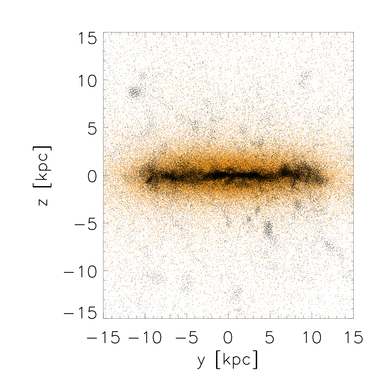
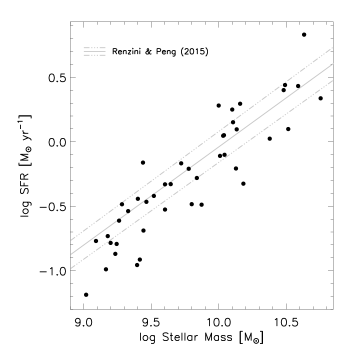
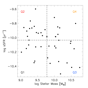
Figure 1: Top row: Positions in physical kpc of gas (black dots) and star (orange dots) particles for the galaxy of the simulated sample with the highest SFR. This object has total (i.e. as determined by SUBFIND) M${}_{\star}=4.30\times 10^{10}$ M_⊙, M${}_{\rm gas}=1.94\times 10^{11}$ M_⊙, M${}_{\rm tot}=1.89\times 10^{12}$ M_⊙, SFR $=6.77$ M_⊙ yr^-1 and $\log\big{(}$sSFR$/$yr${}^{-1}\big{)}=-9.80$. The stellar and gas mass inside the ($30$ kpc)³ cube are, respectively, M${}_{\rm\star,c}=3.51\times 10^{10}$ M_⊙ and M${}_{\rm gas,c}=1.19\times 10^{10}$ M_⊙. Left panel: xz edge-on projection. Middle panel: xy face-on projection. Right panel: yz edge-on projection. Bottom left panel: SFR$-$M_⋆ relation for our simulated galaxies. The grey solid (+ triple dot-dashed) line is the best fit SFR$-$M_⋆ relation for star forming local galaxies of Renzini & Peng (2015). The synthetic sample represents disc galaxies on the main sequence. Bottom right panel: simulated specific SFR$-$M_⋆ relation. The vertical and horizontal dashed lines mark, respectively, the median M_⋆ and sSFR of the final sample: $\log(\tilde{{\rm M}}_{\star}/$M${}_{\odot})=9.78$, $\log(\tilde{\rm sSFR}/$yr${}^{-1})=-10.04$. To facilitate the subsequent analysis, we divided the plot in four quadrants: Q$1$ = low M${}_{\star}-$ low sSFR, Q$2$ = low M${}_{\star}-$ high sSFR, Q$3$ = high M${}_{\star}-$ low sSFR and Q$4$ = high M${}_{\star}-$ high sSFR (see text).

This configuration comes in two different setups: Ref-L025N0752 and Recal-L025N0752. The first one is the initial reference setup, while in the second the subgrid stellar and AGN feedback parameter values were re-calibrated to better match the observed low redshift GSMF (Schaye et al., 2015). In practice, the main difference is that feedback is slightly more effective in Recal. This prevents overcooling problems and leads to more realistic gas and stellar distributions in galaxies. For this reason, we used Recal-L025N0752 for the analysis presented in this paper.

2.3 Galaxy Sample

For this project, we have developed a pipeline to optimise the analysis of EAGLE simulations. The pipeline first (and only once) loads the original EAGLE snapshot and reads the output of SUBFIND (i.e. the catalogue of substructures within DM haloes). Then it extracts and saves only the information needed by the user (e.g. only galaxies with stellar mass, M_⋆, and$/$or specific star formation rate, sSFR $\equiv$ SFR/M_⋆, in a given range, et cetera). Since the original snapshot can be several gigabytes in size, this procedure drastically reduces both memory and time access requirements, speeding up considerably the subsequent analysis.

We used the pipeline to extract cubes of size $30$ physical kpc around all the galaxies with M${}_{\star}\geq 10^{9}$ M_⊙ from Recal-L025N0752 at $z=0$ (taking into account periodic boundary conditions and a buffer of extra $70$ kpc per side for SPH interpolation, see Section 2.4). Each cube is a GADGET format file containing a new header and the following information for gas ($g$) and star ($s$) particles: position ($g$+$s$), velocity ($g$+$s$), mass ($g$+$s$), temperature ($g$), density ($g$), smoothing length ($g$), SFR ($g$), metallicity ($g$+$s$) and age ($s$). The initial sample included $266$ galaxies.

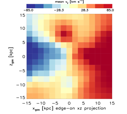
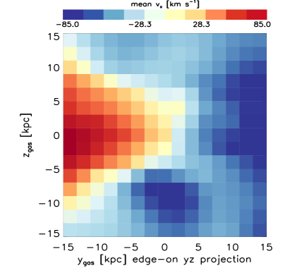
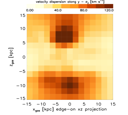
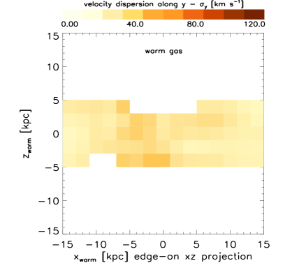
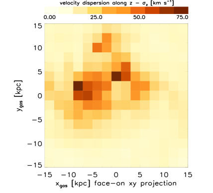
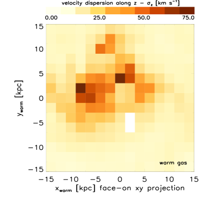
Figure 2: Top row: examples of mean (rotation) velocity maps created using all the gas in the cube. Left panel: edge-on xz projection $-$ mean $v_{\rm y}$. Right panel: edge-on yz projection $-$ mean $v_{\rm x}$. Middle row: gas velocity dispersion maps in the edge-on xz projection $-$ $\sigma_{\rm y}$. Left panel: all gas. Right panel: warm gas, that is only pixels where $3.8\leq\log\big{(}\langle$T${}_{\rm gas}\rangle/$K$\big{)}\leq 4.2$ (see Section 2.4). Warm gas is clearly associated with the galactic disc and virtually absent when moving away from the galaxy plane, where the all gas $\sigma_{\rm y}$-map peaks. Bottom row: gas velocity dispersion maps in the face-on xy projection $-$ $\sigma_{\rm z}$. Left panel: all gas. Right panel: warm gas. Now, all the lines-of-sight pierce the disc (where warm gas dominates) and the two maps are almost identical.

We then rotated the particle distribution ($g$+$s$) around the gravitational potential minimum (using the angular momentum per unit mass of star particles), in order to place each galaxy face-on in the xy plane and edge-on in the xz and yz planes. Accordingly, we rotated the velocity vector of each particle in the cube and used the velocity of the (rotated) stellar centre of mass as the velocity reference frame. At this point, we visually inspected the sample and only selected unperturbed galaxies with a prominent disc structure in both gas and stars, a number of gas particles (N_gas) inside the $30$+$70$ kpc cube sufficient to make our analysis robust, and fairly regular$/$symmetric gas rotation velocity maps (constructed as explained in Section 2.4). The final sample includes $43$ galaxies with $9.02\leq\log($M${}_{\star}/$M${}_{\odot})\leq 10.76$ and $7.8\times 10^{3}\lesssim$ N${}_{\rm gas}\lesssim 9.4\times 10^{4}$ ($\langle$N${}_{\rm gas}\rangle\approx 3.8\times 10^{4}$). In the top row of Fig. 1 we plot positions of gas (black dots) and star (orange dots) particles for the galaxy with the highest SFR. The left and right panels show the edge-on xz and yz projections: the galactic disc is clearly visible in both star and gas components. The middle panel shows the face-on xy projection. The gas distribution is arranged in a complex clumpy structure as a result of the interplay between star formation and associated feedback processes.

The bottom left panel of Fig. 1 shows the distribution in the SFR$-$M_⋆ plane of our final sample of $43$ galaxies. The minimum and maximum star formation rates are $0.065$ and $6.77$ M_⊙ yr^-1. The grey solid (+ triple dot-dashed) line is the best fit SFR$-$M_⋆ relation for star forming local galaxies of Renzini & Peng (2015): $\log\big{(}$SFR$/[$M_⊙ yr${}^{-1}]\big{)}=(0.76\pm 0.01)\log($M${}_{\star}/$M${}_{\odot})-7.64\pm 0.02$. The final sample represents disc galaxies on the main sequence. We plot the simulated specific SFR$-$M_⋆ relation in the bottom right panel of Fig. 1. The vertical and horizontal dashed lines mark, respectively, the median stellar mass, $\log(\tilde{{\rm M}}_{\star}/$M${}_{\odot})=9.78$, and median specific star formation rate, $\log(\tilde{\rm sSFR}/$yr${}^{-1})=-10.04$. In the following sections we will study how the gas velocity dispersion distribution varies as a function of M_⋆ and sSFR. For this reason, we split the plot in four quadrants: Q$1$ = low M${}_{\star}-$ low sSFR, Q$2$ = low M${}_{\star}-$ high sSFR, Q$3$ = high M${}_{\star}-$ low sSFR and Q$4$ = high M${}_{\star}-$ high sSFR. Q$1$ and Q$4$ contain, respectively, $7$ and $8$ galaxies, while both Q$2$ and Q$3$ contain $14$ objects.

2.4 Binning and warm gas

We binned the gas particles in each galactic cube on a $2$D spatial (+ $1$D depth) grid of pixels with linear size $2$ kpc ($15$ pixels per cubic side), which is comparable to the effective resolution of SAMI after accounting for a typical AAT seeing of $2.1$ arcsec. To obtain SPH quantities on the grid, we followed the procedure described in Section 4 of Altay & Theuns (2013). We started by extracting a buffer of additional $70$ kpc per side around the central cube of volume $(30$ kpc$)^{3}$, to ensure that all the gas particles in the simulation whose $3$D SPH kernels intercept one or more pixels of the grid in the $2$ spatial directions and the cube margins in the line-of-sight direction were taken into account. Then, we assigned a truncated Gaussian kernel to each gas particle (Eqs. 8 and 9 of Altay & Theuns 2013) and integrated it over the square pixels. Using this procedure, we calculated the density weighted (mean) velocity, velocity dispersion and temperature along the line-of-sight in all the pixels.

We considered different projections. In the edge-on xz (yz) projection, the line-of-sight direction is the direction y (x) perpendicular to the xz (yz) plane. The corresponding mean velocity and velocity dispersion are, respectively, $v_{\rm y}$ and $\sigma_{\rm y}$ for the xz projection and $v_{\rm x}$ and $\sigma_{\rm x}$ for the yz projection. The velocity dispersion for the face-on projection xy is $\sigma_{\rm z}$. The two top panels of Fig. 2 show examples of mean (rotation) velocity maps in the two edge-on projections created using all the gas in the cube.

SAMI observations of low-redshift galaxies with outflows are largely based on the detection of H$\alpha$ emitting gas at T $\sim 10^{4}$ K. From now on, to better compare with these observations we will distinguish between all gas and warm gas. In an SPH simulation, the fluid conditions at any point are defined by integrating over all particles, weighted by their kernel. Selecting only a subset of them (e.g. only star forming or cold$/$hot gas) would break mass$/$momentum$/$energy conservation laws. Therefore, we define

Warm gas: pixels in a velocity$/$velocity dispersion$/$temperature map where the density weighted gas temperature (calculated using all the particles) is in the range $3.8\leq\log\big{(}\langle$T${}_{\rm gas}\rangle/$K$\big{)}\leq 4.2$.

Gas with temperature around $10^{4}$ K is usually referred to as warm to distinguish it from cold gas in molecular clouds (T $<100$ K) and hot gas in the halo or in supernova bubbles (T $>10^{5}$ K), based on the model of a three-phase ISM medium (McKee & Ostriker, 1977). H$\alpha$ emission in real galaxies is mostly from H ii regions, and hence correlates strongly with star formation rate (Kennicutt, 1998). To a good approximation, in our analysis warm pixels trace pixels with density weighted SFR greater than zero. We introduced this temperature cut to qualitatively compare with the kinematic signatures seen in SAMI observations, without having to model complicated and uncertain radiative transfer effects.

In the middle row of Fig. 2 we plot edge-on velocity dispersion maps (xz $-$ $\sigma_{\rm y}$) for $a$) all gas (left panel) and $b$) warm gas (right panel). In $a$) the velocity dispersion increases when moving away from the disc of the galaxy (in both vertical directions) and peaks at abs(z_gas) $\sim 9$ kpc. On the other hand, in $b$) the high-$\sigma$ part is completely suppressed and warm gas is mainly associated with the galactic disc. This has important consequences for our analysis. We will explore them in Sections 3.1 and 3.2.

The situation is different in the bottom two panels of Fig. 2, which show face-on velocity dispersion maps (xy $-$ $\sigma_{\rm z}$) for all gas (left panel) and warm gas (right panel). This time the two maps are almost identical (except for two pixels). This is due to the fact that now all the lines-of-sight pierce the disc, where warm gas dominates. The $\sigma$-maps in Fig. 2 are the base of all our analyses and we will discuss them more in the next sections.

3 Signatures of outflows: the velocity dispersion distribution

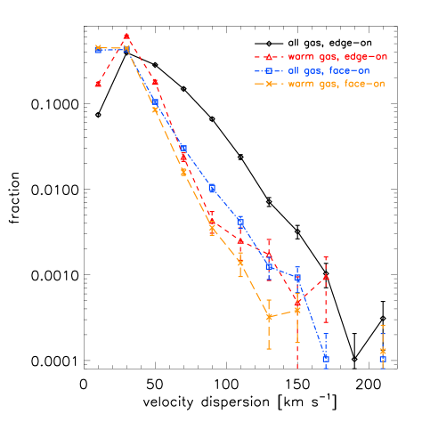
Figure 3: Pixelated velocity dispersion probability distributions (i.e. the fraction of pixels $-$ with pixel size $=2$ kpc $-$ per velocity dispersion bin) calculated using all gas and warm gas in different projections. The bin size is $20$ km s^-1. Black diamonds + solid line and red triangles + short dashed line: all gas and warm gas, respectively, in the edge-on xz projection $-$ $\sigma_{\rm y}$. Blue squares + dot-dashed line and orange crosses + long dashed line: all gas and warm gas, respectively, in the face-on xy projection $-$ $\sigma_{\rm z}$. Each line was created by stacking the histograms of all the $43$ galaxies in the simulated sample. Errors are Poissonian. Since in the face-on projection the lines-of-sight in different pixels always pierce the galactic disc, where warm gas dominate, the all gas and warm gas $\sigma_{\rm z}$-distributions are very similar (see the bottom panels of Fig. 2). In the edge-on projection, the $\sigma_{\rm y}$-distribution for all gas is shifted to higher velocity dispersions than the warm gas distribution, which is associated with the galactic disc and therefore has a more prominent peak at low $\sigma_{\rm y}=30$ km s^-1 (cf. the two middle panels of Fig. 2).

The aim of this work is to determine whether or not current and upcoming IFS surveys can succesfully identify large-scale outflows and provide meaningful constraints on the physical processes driving gas out of galaxies. For this reason, we apply observationally-based analysis techniques to the simulations. In particular, in the next sections we compare with the observational investigations of SAMI galaxies with outflows presented by Ho et al. (2014) and Ho et al. (2016b). We stress that observational and numerical analyses estimate the kinematic state of the gas in two different ways. We track the motion of particles as sampled by the SPH scheme in the simulation, without including any radiative transfer effects. Instead, Ho et al. (2014, 2016b) extract kinematic information from emission line spectra of galaxies. Thus, while observations only probe ionised gas, simulations take into account all the gas in the galactic halo. To facilitate the comparison, we therefore introduced in the previous section the definition of warm gas that we will use throughout the paper.

Ho et al. (2014) studied the nature of a prototypical low redshift isolated disc galaxy with outflows: SDSS J$090005.05$+$000446.7$ (SDSS J$0900$, $z=0.05386$). Its emission line spectrum was decomposed using the spectral fitting pipeline LZIFU (Ho et al., 2016a), a likelihood ratio test and visual inspection. Emission lines were modelled as Gaussians composed of up to three kinematic components with small, intermediate and high velocity dispersion relative to each other (i.e from narrow to broad features). Fig. 6 of Ho et al. (2014) shows the velocity dispersion distribution of SDSS J$0900$. The statistically prominent narrow component peaks at $\sim 40$ km s^-1 and is associated with the (rotationally supported) disc of the galaxy. More interestingly, the $\sigma$-distribution extends to very high values ($450$ km s^-1) with the broad kinematic component peaking at $\sim 300$ km s^-1. The authors argue that this high-$\sigma$ component traces shock excited emission in biconical outflows, likely driven by starburst activity.

3.1 All gas vs warm gas

Following Ho et al. (2014), we begin our analysis by investigating the velocity dispersion distribution of the simulated galaxies. Throughout the paper, we adopt the following procedure. Using $\sigma$-maps like those shown in the bottom four panels of Fig. 2, we first calculate the histogram of the pixelated velocity dispersion for each galaxy (i.e. the fraction of pixels per velocity dispersion bin), where the pixel size is $2$ kpc, the upper limit is the maximum $\sigma$ of the entire sample (that changes depending on the projection and if all gas or warm gas is considered) and the bin size is always $20$ km s^-1. Then, we stack these histograms and normalize by the number of galaxies to obtain the final pixelated velocity dispersion (probability) distribution and its associated Poissonian errors.

In Fig. 3 we examine the differences between the pixelated velocity dispersions calculated using all gas and warm gas in different projections for all the $43$ simulated galaxies. In the face-on (xy view) projection, the $\sigma_{\rm z}$-distributions of all gas (blue squares and dot-dashed line) and warm gas (orange crosses and long dashed line) are very similar, with the highest fractions at low $\sigma_{\rm z}$ and a declining trend at larger velocity dispersions, and share the same $\max(\sigma_{\rm z})=201.31$ km s^-1. The only difference is that the all gas distribution shows slightly larger statistics at high $\sigma_{\rm z}$. According to the bottom panels of Fig. 2, this is not surpising. When the lines-of-sight in different pixels pass through the galactic disc, particles in the warm gas regime are the majority and dominate the $\sigma_{\rm z}$-maps.

On the other hand, the edge-on (xz view) $\sigma_{\rm y}$-distribution for all gas (black diamonds and solid line, $\sigma_{\rm y,\max}=211.08$ km s^-1) is shifted to higher velocity dispersions than the warm gas distribution (red triangles and short dashed line, $\sigma_{\rm y,\max}=169.29$ km s^-1), which has a more prominent peak at $30$ km s^-1 and then rapidly drops to lower fractions at high $\sigma_{\rm y}$. The reasons for this are mentioned in Section 2.1 and highlighted by the two middle panels of Fig. 2. In our simulated disc galaxies, warm gas traces the disc and is virtually absent when moving away from the galaxy plane. In Section 3.3, we will show how the extraplanar velocity dispersion is dominated by outflowing gas. Therefore, the lack of warm gas outside the disc is a direct consequence of the thermal stellar feedback implemented in EAGLE that heats outflowing particles up to a temperature higher than the warm range (T $\sim 10^{4}$ K). Galactic winds in our simulations are mostly hot (T $>10^{5}$ K) and, compared to observed galaxies, may entrain insufficient gas with T $<10^{5}$ K. Note that such high-temperature gas would not be visible in SAMI observations.

This issue with EAGLE was already noted by Turner et al. (2016) in a study of the $z\approx 3.5$ intergalactic medium and has important implications for our work too. A direct comparison with H$\alpha$-based SAMI observations should be done using warm gas (since H$\alpha$ emitting gas has a temperature T $\sim 10^{4}$ K). However, the paucity of such gas in the outflows of our simulated galaxies could lead to misleading results. Specifically, in edge-on projections: underestimation of the outflowing gas mass$/$incidence of galactic winds (that may be there but just too hot to be detected in H$\alpha$) and poor sampling of the extraplanar gas. In the next section we will show an example of this problem.

3.2 Disc component and off-plane gas

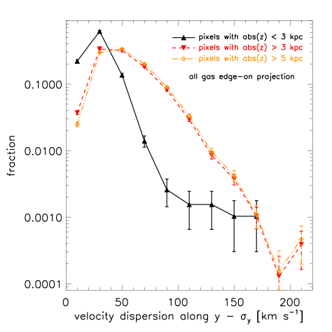
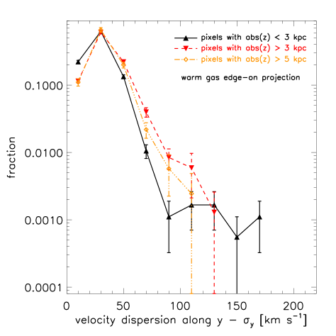
Figure 4: Pixelated velocity dispersion probability distributions (cf. Fig. 3 and the beginning of Section 3.1) calculated by assuming different cuts in the z direction of the edge-on (xz view) $\sigma_{\rm y}$-maps (with pixel size $=2$ kpc) to separate the galactic disc component from the extraplanar one. Left panel: all gas. Right panel: warm gas. Black filled triangles and solid line, (internal) pixels with abs(z) $<$ $3$ kpc. Red filled inverted triangles and dashed line, (external) pixels with abs(z) $>$ $3$ kpc. Orange diamonds and triple dot-dashed line, (external) pixels with abs(z) $>$ $5$ kpc. Errors are Poissonian. In the all gas case, excluding the galactic disc shifts the $\sigma_{\rm y}$-distribution to larger velocity dispersions. In the warm gas case, the off-plane distributions are poorly sampled and only marginally different from the disc one due to the scarcity of extraplanar gas at T $\sim 10^{4}$ K.

We focus on the difference between gas in the disc and extraplanar gas. To do so, we take the edge-on $\sigma_{\rm y}$-maps (xz view) and restrict the number of pixels in the direction perpendicular to the disc plane by applying various vertical cuts. The resulting pixelated velocity dispersion distributions (including Poissonian errors) are shown in Fig. 4. The two panels refer to all gas (left) and warm gas (right).

In the left panel, when all gas and only pixels with abs(z) $<$ $3$ kpc (black filled triangles and solid line) are included, the distribution shows a sizeable peak at $\sigma_{\rm y}=30$ km s^-1 and then quickly declines to low fractions. With this pixel selection, we are targeting only a thin layer of gas in the edge-on galactic discs. Red filled inverted triangles and the dashed line represent the complementary distribution calculated using only pixels with abs(z) $>$ $3$ kpc. In this case, the distribution is shifted to larger $\sigma$-values than before, while the low-$\sigma$ part is greatly reduced. This demonstrates that the low-$\sigma$ peak is indeed associated mainly with the galactic disc, in qualitative agreement with Ho et al. (2014). In the left panel of Fig. 4 we also show the velocity dispersion distribution (for all gas) calculated using only pixels with abs(z) $>$ $5$ kpc (orange diamonds and triple dot-dashed lines). The low-$\sigma$ peak and high-$\sigma$ tail become, respectively, slightly less and more important when moving further away from the galactic disc, supporting our previous conclusion.

The right panel of Fig. 4 illustrates how using only warm gas can be misleading, in the framework of EAGLE simulations. All three distributions are very similar (despite the fact that they probe rather different environments) and more noisy at $\sigma_{\rm y}>50$ km s^-1 than the corresponding distributions for all gas. In the edge-on warm $\sigma_{\rm y}$-maps there are only a few pixels with abs(z) $>$ $3$ and (especially) $5$ kpc, therefore poor sampling affects the results in these two cases. Considering only warm gas in EAGLE would lead to the wrong conclusion that planar and extraplanar gas components are kinematically similar. This is a consequence of the thermal implementation of stellar feedback that produces hot outflows. When all gas (warm & hot) is considered, the extraplanar (mainly hot) gas is kinematically clearly distinct from the (mainly warm) disc (left panel of Fig. 4).

In the rest of the paper, whenever possible and appropriate (e.g. to study face-on velocity dispersion distributions or the impact of general galactic properties like M_⋆ and sSFR) we will show results obtained using warm gas. However, including all gas will be necessary to ensure a robust description of galactic winds and outflow signatures (see e.g. Section 5).

3.3 Outflows

In the previous section we have demonstrated how the low-$\sigma$ part of the edge-on velocity dispersion distribution is associated with the galactic disc. Now, we study the origin of the high-$\sigma$ tail. In the xz edge-on projection, we consider a pixel of the $\sigma$-map as outflow dominated if the density weighted vertical velocity of its gas particles, $\langle v_{\rm z}\rangle$, is positive in the semi-plane with z${}_{\rm gas}>0$ kpc or negative in the negative z_gas semi-plane (i.e. if the gas particles contributing to the pixel are predominantly moving away from the galactic plane). Otherwise, a pixel is flagged as non-outflow dominated. The corresponding $\sigma_{\rm y}$-distributions are shown in Fig. 5. Errors are Poissonian.

The non-outflow dominated $\sigma$-distribution (black diamonds and solid line) resembles the abs(z) $<$ $3$ kpc distribution (i.e. associated with the galactic disc) visible in the left panel of Fig. 4 (black filled triangles and solid line). With respect to these two diagrams, the outflow dominated $\sigma$-distribution of Fig. 5 (red triangles and dashed line) is shifted to higher velocity dispersions and has a more statistically prominent high-$\sigma$ tail (in agreement with the abs(z) $>$ $3$ and $5$ kpc distributions of Fig. 4). When only extraplanar gas is considered (i.e. pixels with abs(z) $>$ $3$ kpc), we find that in $42$ out of $43$ simulated galaxies, the number of outflow dominated pixels is greater than the number of non-outflow dominated pixels. On average, this excess is a factor of $\sim 3.2$ times and can be up to $>15$ times.

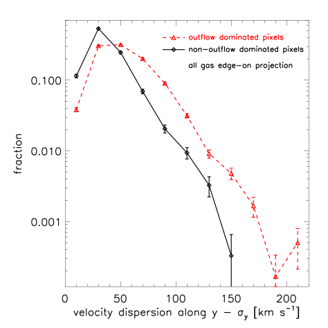
Figure 5: Pixelated velocity dispersion probability distributions (cf. Fig. 3 and the beginning of Section 3.1) for outflow dominated (red triangles and dashed line) and non-outflow dominated (black diamonds and solid line) pixels. Errors are Poissonian and we consider all gas in the edge-on xz projection $-$ $\sigma_{\rm y}$. The velocity dispersion distribution based on outflow dominated pixels is more prominent at high-$\sigma$.

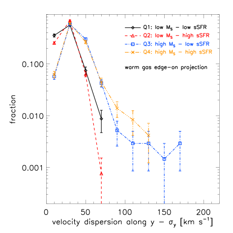
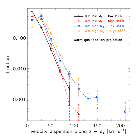
Figure 6: Pixelated velocity dispersion probability distributions (cf. Fig. 3 and the beginning of Section 3.1) for galaxies in the four M${}_{\star}-$sSFR quadrants defined in the bottom right panel of Fig. 1: Q$1$ = low M${}_{\star}-$ low sSFR, Q$2$ = low M${}_{\star}-$ high sSFR, Q$3$ = high M${}_{\star}-$ low sSFR and Q$4$ = high M${}_{\star}-$ high sSFR. Left panel: edge-on xz projection $-$ $\sigma_{\rm y}$. Right panel: face-on xy projection $-$ $\sigma_{\rm z}$. Errors are Poissonian and we consider only warm gas. In general, galaxies with higher M_⋆ present a more extended $\sigma$-distribution, while the sSFR has a secondary effect with respect to stellar mass.

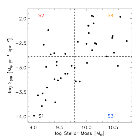
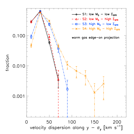
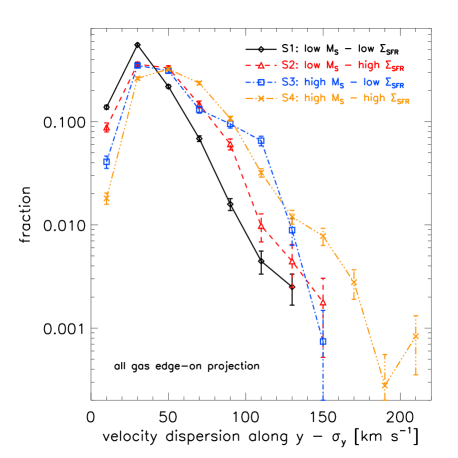
Figure 7: Top panel: relation between star formation rate surface density, $\Sigma_{\rm SFR}$, and M_⋆ for our simulated galaxies. $\Sigma_{\rm SFR}={\rm SFR}/(2\pi r_{50}^{2})$, where SFR is the total star formation rate and $r_{50}$ is the radius within which half of the galaxy stellar mass is included. The plot is divided in four sectors: S$1$ = low M${}_{\star}-$ low $\Sigma_{\rm SFR}$, S$2$ = low M${}_{\star}-$ high $\Sigma_{\rm SFR}$, S$3$ = high M${}_{\star}-$ low $\Sigma_{\rm SFR}$ and S$4$ = high M${}_{\star}-$ high $\Sigma_{\rm SFR}$ (see Section 4.1). Bottom panels: pixelated velocity dispersion probability distributions (cf. Fig. 3 and the beginning of Section 3.1) for galaxies in the four sectors defined in the top panel. Errors are Poissonian. We only consider the edge-on xz projection $-$ $\sigma_{\rm y}$. Left panel: warm gas. As in the previous section, a trend with stellar mass is visible. Right panel: all gas. At fixed M_⋆, galaxies with high $\Sigma_{\rm SFR}$ give rise to a $\sigma$-distribution shifted to larger velocity dispersions compared to galaxies with low $\Sigma_{\rm SFR}$.

Our results are qualitatively consistent with the observations of Ho et al. (2014): in low redshift disc galaxies, the low-$\sigma$ component of the velocity dispersion distribution is associated with the (rotationally supported) disc, while the high-$\sigma$ component mainly traces extraplanar, outflowing gas. In the case of strong disc-halo interactions through galactic winds, the velocity dispersion of the extraplanar gas is broadened (up to $300$ km s^-1 in the extreme case of M82) by both the turbulent motion of the outflowing gas and line splitting caused by emissions from the approaching and receding sides of the outflow cones (Ho et al., 2016b, and references therein).

There is an important caveat to consider here. In this work, outflowing material includes both particles that are actually leaving their host galaxy and particles that will eventually stop and fall back to the disc. At this stage, our numerical analysis is not able to differentiate between these two components (but this also applies to observations). Theoretical predictions on how much gas actually escapes from galaxies are crucial, since the escaping mass is very hard to measure observationally (Bland-Hawthorn & Cohen, 2003; Bland-Hawthorn et al., 2007). Recent simulations run by different groups indicate that wind recycling becomes particularly important at $z<1$ and galaxies of all masses reaccrete more than $50$% of the expelled gas (e.g. Oppenheimer et al., 2010; Nelson et al., 2015; Christensen et al., 2016; Anglés-Alcázar et al., 2017). This point will be addressed in an upcoming paper (Crain et al. in prep). Note that the thermal$/$buoyant winds in our EAGLE discs will allow particles without enough velocity$/$thermal energy to escape to float up to the top of the galactic halo (Bower et al., 2017).

4 Impact of stellar mass, specific SFR, SFR surface density and gas temperature

In this section, we study the impact of different galactic properties on the overall shape of the velocity dispersion distribution. Since we do not focus primarily on the high-$\sigma$ tail associated with outflows, results are presented for warm gas to better compare with the observational analysis of Ho et al. (2014, 2016b). We begin with stellar mass and the specific star formation rate. Fig. 6 shows the result: the edge-on xz projection $-$ $\sigma_{\rm y}$ in the left panel and the face-on xy projection $-$ $\sigma_{\rm z}$ in the right panel (errors are Poissonian). We divided our galaxies according to the four M${}_{\star}-$sSFR quadrants in the bottom right panel of Fig. 1 (the same colour code applies).

A clear trend with stellar mass is visible in both panels, while the sSFR appears to have a secondary effect. It is interesting to note how, especially in the edge-on projection (left panel), the velocity dispersion distribution of low mass galaxies (black diamonds + solid line and red triangles + dashed line, respectively associated with Q$1$ and Q$2$) declines shortly after the peak at $30$ km s^-1 (associated with the disc) and drops to zero already at $70$ km s^-1. The predominance of the disc component in Q$1$ and Q$2$ is present also when all gas distributions (not shown here) are used. The $\sigma$-distributions of galaxies with high-M_⋆ (blue squares + dot-dashed line and orange crosses + triple dot-dashed line, respectively associated with Q$3$ and Q$4$) are more extended, and prominent at high-$\sigma$, than those of low mass galaxies (regardless of the range in sSFR). At $\sigma<100$ km s^-1, this is due to the fact that in the synthetic sample warm gas mainly traces the galactic disc and objects in Q$3$ and Q$4$ are generally bigger. Due to the SFR$-$M_⋆ relation and the fact that in EAGLE there is a direct connection between SFR and stellar feedback, these objects also have higher outflowing activities than galaxies in Q$1$ and Q$2$. Despite the lack of warm gas in EAGLE’s galactic winds, this causes the broadening of the $\sigma$-distributions to higher velocity dispersion.

Our simulated face-on distributions, with $\max(\sigma_{\rm z})=201.31$ km s^-1, do not extend as far as the velocity dispersion diagram of the SDSS J$0900$ galaxy in Ho et al. (2014), with $\max(\sigma_{\rm z})\sim 450$ km s^-1. This might be in part due to the fact that SDSS J$0900$ is more massive, $\log($M${}_{\star}/$M${}_{\odot})=10.8$, and has a higher SFR ($\sim 5-15$ M_⊙ yr^-1, depending on the adopted SFR indicator) than objects in our synthetic sample, but could also indicate that the effect of EAGLE stellar feedback on gas kinematics is too weak. Simulated galaxies in Q$2$, Q$3$ and Q$4$ have distributions that reach $\sigma_{\rm z}>100$ km s^-1, which is the starting point of the broad kinematic component associated with outflowing gas in SDSS J$0900$.

4.1 SFR surface density

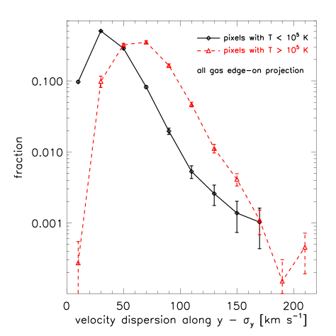
Figure 8: Left panel: average temperature distribution of gas particles inside cubes of linear size $30$ kpc centred on each simulated galaxy. Two distinct regions are visible in the gas temperature histogram: the bulk of particles with T $<10^{5}$ K, and a tail of particles with T $\geq 10^{5}$ K. Right panel: effect of gas temperature on the pixelated velocity dispersion probability distribution (cf. Fig. 3 and the beginning of Section 3.1) of galaxies. Black diamonds and solid line: pixels where the density weighted gas temperature is T $<10^{5}$ K. Red triangles and dashed line: pixels with T $\geq 10^{5}$ K. Errors are Poissonian and we only consider the edge-on xz projection $-$ $\sigma_{\rm y}$. Pixels with temperature T $<10^{5}$ K trace the galactic disc (low-$\sigma$), while those with T $\geq 10^{5}$ K are associated with higher-$\sigma$ (i.e. extraplanar, outflowing gas).

Ho et al. (2016b) found that, on average, wind galaxies have higher star formation rate surface densities than those without strong wind signatures. We checked this result with our simulated sample in Fig. 7. Following Ho et al. (2016b), the star formation rate surface density is defined as $\Sigma_{\rm SFR}=$ SFR$/(2\pi r_{50}^{2})$, where SFR is the total star formation rate of the object as determined by SUBFIND and $r_{50}$ is the radius within which half of the galaxy stellar mass is included. The top panel of Fig. 7 shows the $\Sigma_{\rm SFR}-$M_⋆ relation of EAGLE galaxies. As for SFR and M_⋆, the two quantities are positively correlated. The vertical and horizontal dashed lines mark, respectively, the median stellar mass, $\log(\tilde{{\rm M}}_{\star}/$M${}_{\odot})=9.78$, and median star formation rate surface density, $\log\big{(}\tilde{\rm\Sigma}_{\rm SFR}/[$M_⊙ yr^-1 kpc${}^{-2}]\big{)}=-2.77$. We divided the plot in four sectors: S$1$ = low M${}_{\star}-$ low $\Sigma_{\rm SFR}$ (16 objects), S$2$ = low M${}_{\star}-$ high $\Sigma_{\rm SFR}$ (5 objects), S$3$ = high M${}_{\star}-$ low $\Sigma_{\rm SFR}$ (6 objects) and S$4$ = high M${}_{\star}-$ high $\Sigma_{\rm SFR}$ (16 objects). The corresponding velocity dispersion distributions are shown in the bottom panels of Fig. 7: warm gas on the left and all gas on the right (we only consider the edge-on xz projection $-$ $\sigma_{\rm y}$).

We start by considering the warm gas case (left panel of Fig. 7). Trends are similar to those of the left panel of Fig. 6. At low masses (S$1$ and S$2$), the velocity dispersion distributions of galaxies with low and high $\Sigma_{\rm SFR}$ are almost identical (black diamonds + solid line and red triangles + dashed line), with a narrow peak at $30$ km s^-1. These galaxies have relatively low SFRs and weak outflowing activities, therefore warm gas mainly traces their galactic discs (of similar size). The probability distributions of high-mass galaxies (blue squares + dot-dashed line and orange crosses + triple dot-dashed line, respectively associated with S$3$ and S$4$) are shifted to larger values than those of low-mass galaxies. As discussed in the previous section, part of the shift is driven by the increase in stellar mass, but a correlation with the SFR surface density is now visible (a more extended high-$\sigma$ tail for objects in S$4$ with high $\Sigma_{\rm SFR}$).

Patterns are different in the all gas case (right panel of Fig. 7). A trend with stellar mass is still present (black & red vs blue & orange points and lines), but, at fixed M_⋆, galaxies with high $\Sigma_{\rm SFR}$ give rise to a $\sigma$-distribution shifted to larger velocity dispersions compared to galaxies with low $\Sigma_{\rm SFR}$ (red & orange vs black & blue points and lines). As in the observations of Ho et al. (2016b), this result, only partially visible before due to the lack of warm gas in the outflows of EAGLE galaxies, indicates that the star formation rate surface density correlates with the outflowing activity even when $\Sigma_{\rm SFR}$ is rather low, as it is the case of our simulated galaxies (we will explore the correlation in more detail in Section 5). According to Heckman (2002), starburst-driven winds are observed to be ubiquitous in galaxies with $\log\big{(}\Sigma_{\rm SFR}/[$M_⊙ yr^-1 kpc${}^{-2}]\big{)}>-1$ (see also the results of Sharma et al., 2017). In our sample, $\log\big{(}\Sigma_{\rm SFR,\max}/[$M_⊙ yr^-1 kpc${}^{-2}]\big{)}=-1.95$, almost a dex lower.

4.2 The role of gas temperature

Since the predictive power of realistic numerical simulations allows us to study the effect of additional galactic properties, which are usually hard to measure observationally, we looked for a way to better relate the shape of the velocity dispersion distribution to feedback processes. In EAGLE, stellar feedback is implemented thermally, and we found that temperature is a good proxy to distinguish low- and high-$\sigma$ parts in our simulated galaxies. The average temperature histogram of gas particles inside cubes of volume ($30$ kpc)³ centred on each simulated galaxy splits into two regions: the bulk of particles with T $<10^{5}$ K, and a tail of particles with T $\geq 10^{5}$ K (see the left panel of Fig. 8). For this reason, we divided pixels in the velocity dispersion distribution where the density weighted gas temperature is above and below $10^{5}$ K. The result is visible in the right panel of Fig. 8 (we consider all gas in the edge-on xz projection $-$ $\sigma_{\rm y}$, errors are Poissonian). The condition on temperature produces two very different probability distributions. When pixels with T $<10^{5}$ K are selected (black diamonds and solid line), the distribution peaks at $\sigma_{\rm y}=30$ km s^-1, then quickly drops to low fractions. On the other hand, pixels with T $\geq 10^{5}$ K give rise to a distribution shifted to larger velocity dispersions and where the low-$\sigma$ section is less prominent (red triangles and dashed line). These trends, which we find are also visible in the face-on xy projection $-$ $\sigma_{\rm z}$, support the results of the previous sections (see in particular the left panel of Fig. 4 and Fig. 5).

Thus, EAGLE simulations of low redshift disc galaxies indicate a direct correlation between the thermal state of the gas and its state of motion as described by the velocity dispersion distribution:

• Low-$\sigma$ peak $\,\,\Leftrightarrow\,$ galactic disc$/$gas with T $<10^{5}$ K;

• High-$\sigma$ tail $\,\Leftrightarrow\,$ outflows$/$gas with T $\geq 10^{5}$ K.

The real picture is certainly more complicated than this. For example, blobs of cold gas at relatively high density could be entrained in hot, diffuse winds (Veilleux et al., 2005; Cooper et al., 2008, 2009). Despite the simplifications made in our analysis, the predicted correlation between EAGLE’s thermal$/$buoyant outflows and high temperature gas can be very useful to guide and interpret real observations.

5 SIGNATURES OF WINDS: GAS KINEMATICS IN EAGLE AND SAMI GALAXIES

Ho et al. (2016b) proposed an empirical identification of wind-dominated SAMI galaxies. In this section, we apply the same methodology to our simulated sample. The authors defined two dimensionless quantities to measure the (ionised gas) extraplanar velocity dispersion and asymmetry of the velocity field. The first quantity is the velocity dispersion to rotation ratio parameter:

$$\eta_{50}=\sigma_{50}/v_{\rm rot},$$ (1)

where $\sigma_{50}$ is the median velocity dispersion of all pixels outside $\tilde{r}_{\rm e}$ (the $r$-band effective radius increased by approximately 1 arcsec to reduce the effect of beam smearing) with signal-to-noise in H$\alpha$ $-$ S$/$N(H$\alpha$) $-$ greater than $5$. $v_{\rm rot}$ is the maximum rotation velocity measured from the pixels along the optical major axis (for galaxies without sufficient spatial coverage, they used the stellar mass Tully-Fisher relation to infer $v_{\rm rot}$). The second quantity is the asymmetry parameter:

$$\xi={\rm std}\,\bigg{(}\frac{v_{\rm gas}-v_{\rm gas,flipped}}{\sqrt{{\rm Err}(v_{\rm gas})^{2}+{\rm Err}(v_{\rm gas,flipped})^{2}}}\bigg{)},$$ (2)

where ${\rm std}=$ standard deviation. To obtain $\xi$, the authors first flipped the line-of-sight velocity map over the galaxy major axis, $v_{\rm gas,flipped}$, and then subtracted the flipped map from the original one, $v_{\rm gas}$. ${\rm Err}(v_{\rm gas})$ and ${\rm Err}(v_{\rm gas,flipped})$ are the corresponding $1\sigma$ error maps from LZIFU. The standard deviation is again calculated taking into account only pixels outside $\tilde{r}_{\rm e}$ with S$/$N(H$\alpha$) $>5$.

Ho et al. (2016b) used $\eta_{50}$ and $\xi$ to quantify the strength of disc-halo interactions and to distinguish galactic winds from extended diffuse ionised gas (eDIG) in a sample of $40$ low redshift disc galaxies. Since galactic winds both perturb the symmetry of the extraplanar gas velocity and increase the extraplanar emission line widths, they should show high $\xi$ and high $\eta_{50}$. On the other hand, eDIG is more closely tied to the velocity field of the galaxy and therefore should result in low $\xi$ and low $\eta_{50}$.

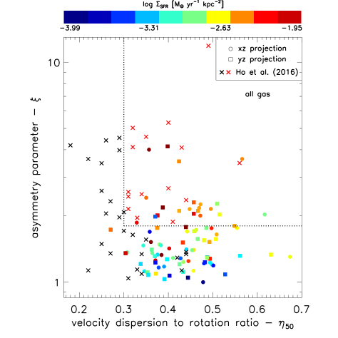
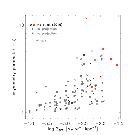
Figure 9: Left panel: asymmetry parameter $\xi$ vs velocity dispersion to rotation ratio parameter $\eta_{50}$. Dots: simulated edge-on xz projection. Squares: simulated edge-on yz projection. Synthetic data are colour coded according to the SFR surface density of the parent galaxy, $\Sigma_{\rm SFR}={\rm SFR}/(2\pi r_{50}^{2})$. The vertical and horizontal dotted lines mark the observational limits above which galaxies show strong disc-halo interactions according to Ho et al. (2016b), $\eta_{50}>0.3$ and $\xi>1.8$. Crosses: observational SAMI data, where red x symbols represent wind-dominated galaxies and black x symbols represent galaxies without strong wind signatures. Right panel: correlation between the asymmetry parameter $\xi$ and $\Sigma_{\rm SFR}$. Grey dots and squares: simulated galaxies in the edge-on xz and yz projections, respectively. Crosses: observational data from Ho et al. (2016b). In both panels, the range of the simulated parameters (determined using all gas) is broadly consistent with the observations. A clear positive $\xi-\Sigma_{\rm SFR}$ correlation is visible in both EAGLE and SAMI data.

We calculated $\eta_{50}$ and $\xi$ for our simulated galaxies and plot them (dots and squares) along with the observational data (black$/$red crosses) in Fig. 9. We remind the reader that there are some differences between the two analyses. The underlying assumptions are the same (i.e. regular, not warped discs and rotation maps, exclusion of mergers and systems undergoing major interactions) but, for example, ${\rm Err}(v_{\rm gas})$ and ${\rm Err}(v_{\rm gas,flipped})$ in Eq. 2 are undefined in our analysis of EAGLE galaxies, since we rely on the SPH scheme to directly determine the kinematic state of the gas, without performing any emission line fitting. Instead, to obtain an estimate of the noise consistent with SAMI data, we fit a polynomial to Ho et al. (2016b)’s ${\rm Err_{\rm obs}}(v_{\rm gas})-$z [kpc] scatter plot and then add the observational noise to the simulated velocity maps. Note that the error on $v_{\rm gas}$ increases with the distance from the galaxy plane because the S$/$N of extraplanar H$\alpha$ emission is lower than that of H$\alpha$ gas in the disc. Furthermore, observations only consider ionised gas, while we take into account all (warm + hot) gas in the galactic cubelet to better sample any outflowing activity (see Sections 3.1 and 3.2). Despite these differences, the range in $\eta_{50}$ and $\xi$ is similar in simulations and observations.

Ho et al. (2016b) empirically defined as wind-dominated those galaxies with $\eta_{50}>0.3$ and $\xi>1.8$. These limits are visible in the left panel of Fig. 9 as the vertical and horizontal black dotted lines. Accordingly, red x symbols in the figure represent wind-dominated SAMI galaxies ($15$ out of $40$), while black x symbols are associated with ($25$) observed objects without strong wind signatures. Among the EAGLE galaxies, just one object has $\eta_{50}<0.3$ (and only in the yz projection value). Although this would be consistent with a wind-dominated galaxy sample, the range in $\xi$ does not support this conclusion. The mean asymmetry parameter is $1.63$ (below the threshold of Ho et al. 2016b) and only five discs have $\xi>1.8$ in both projections.

We are interested in studying the interdependency between $\eta_{50}$, $\xi$ and relevant galactic properties. As for the observational sample, the Spearman rank correlation test indicates no significant correlation between the two parameters: $\rho=0.12$ with a significance of $0.27$. Ho et al. (2016b) argue that if winds are the only mechanism disturbing the extraplanar gas, then a trend between $\eta_{50}$ and $\xi$ should be expected. The fact that both works fail to find a significant correlation suggests that, when applied to current data and simulations, the $\xi-\eta_{50}$ plot might not be accurate enough for the identification of wind-dominated galaxies. Ho et al. (2016b) speculate that gas accreted on to galaxies through satellite accretion would cause a large velocity asymmetry of the extraplanar gas without affecting much the off-plane velocity dispersion (i.e. large $\xi$ and small $\eta_{50}$), and therefore complicate the interpretation of the $\xi-\eta_{50}$ plot in terms of galactic winds and eDIG. We saw in Section 3.3 how the extraplanar gas distribution of EAGLE objects is dominated by outflows (the ratio of outflow to non-outflow dominated pixels is on average $\sim 3.2$). Unfortunately, this does not lead to a significant $\xi-\eta_{50}$ correlation in the simulated sample.

However, Fig. 9 highlights a different trend within EAGLE and SAMI data. In the left panel, simulations are colour coded according to the SFR surface density of the parent galaxy, $\Sigma_{\rm SFR}={\rm SFR}/(2\pi r_{50}^{2})$. In general, objects with low$/$high $\xi$ have low$/$high $\Sigma_{\rm SFR}$ (i.e. bluish points are below reddish points). This positive correlation is even more visible in the right panel of Fig. 9, where we plot $\xi$ as a function of $\Sigma_{\rm SFR}$. The Spearman rank correlation test indicates a significant correlation between the two parameters both in simulations (grey dots and squares, $\rho=0.67$ with a significance of $\sim 10^{-6}$) and observations (black$/$red crosses, $\rho=0.56$ with a significance of $1.6\times 10^{-4}$). Since the asymmetry parameter marks the incidence of galactic winds in disc galaxies, this result is in qualitative agreement with Section 4.1 and the conclusions of Ho et al. (2016b): the star formation rate surface density correlates with outflowing activity.

At this point, it is important to remark that numerical results could be affected by statistical noise in various ways. For example, in low mass, small galaxies high asymmetry could be due to poor sampling of the extraplanar gas distribution, rather than galactic winds. Moreover, since our discs are fairly regular, the two sets of $\eta_{50}$ and $\xi$ parameters associated with the edge-on xz and yz projections should contain the same information, and therefore be statistically similar. However, the analysis is limited by the small size of the synthetic sample ($43$ galaxies), which is due to the small box size of the cosmological simulation used ($25$ cMpc). In principle, increasing resolution and box size of the simulations will alleviate the impact of statistical noise.

Note that the position of SAMI galaxies in the $\xi-\eta_{50}$ plot can also be biased in different ways. For example, see the discussion in Ho et al. (2016b) on how, for galaxies without a direct measurement of $v_{\rm rot}$, the lack of correlation between $\xi$ and $\eta_{50}$ is partially due to the scatter in the Tully-Fisher relation. Furthermore, the high asymmetry seen in some of the observed galaxies might be accentuated by inclination effects (while all the simulated galaxies are perfectly edge-on).

In summary, according to our analysis, the $\xi-\eta_{50}$ plot does not seem to provide a clear, unambiguous tool to identify wind-dominated galaxies. Although using simulations with higher resolution (and better quality observational data) could improve the results, different observables (e.g. the velocity dispersion distribution) appear to estimate the outflowing activity of star forming galaxies more accurately than $\xi$ and $\eta_{50}$.

6 Conclusions

In this paper we have presented an analysis of stellar feedback-driven galactic outflows based on the comparison between hydrodynamic simulations and IFS observations from the SAMI survey (Bryant et al., 2015). We have extracted cubes of $30$ physical kpc around unperturbed disc galaxies from the highest resolution cosmological simulation of the EAGLE set (Schaye et al., 2015). Our final sample includes $43$ main sequence objects with $9.02\leq\log($M${}_{\star}/$M${}_{\odot})\leq 10.76$ and $\log(\tilde{\rm sSFR}/$yr${}^{-1})=-10.04$ (Fig. 1). We have divided each cubelet into a grid of pixel size $2$ kpc (which is comparable to the effective resolution of SAMI) and created gas rotation velocity and velocity dispersion maps (Fig. 2). In our study the terms galactic winds and outflows are synonyms that we have used to identify both gas in the process of leaving a galaxy and gas that will eventually stop and fall back to the disc.

This work is the theoretical counterpart of the observational analyses on SAMI galaxies with outflows presented in Ho et al. (2014) and Ho et al. (2016b). In the first part of the paper, we have focussed on the pixelated velocity dispersion (probability) distribution as a tracer of galactic wind signatures. To better compare with SAMI observations that mainly target H$\alpha$ emitting gas at T $\sim 10^{4}$ K, we have distinguished between all gas and warm gas. The latter identifies pixels in a velocity$/$velocity dispersion$/$temperature map where the density weighted gas temperature (calculated using all the particles) is in the range $3.8\leq\log\big{(}\langle$T${}_{\rm gas}\rangle/$K$\big{)}\leq 4.2$. We have found that, in EAGLE galaxies, warm gas traces the disc and is virtually absent when moving away from the galaxy plane (middle two panels of Fig. 2). For this reason, the edge-on velocity dispersion for warm gas has a less prominent high-$\sigma$ tail (that is mostly associated with outflows) and a lower $\sigma_{\max}$ than the all gas distribution, while the two face-on distributions are very similar (Fig. 3). The lack of warm gas outside the disc is a direct consequence of the thermal stellar feedback implemented in EAGLE. Galactic winds in our simulations are mostly hot (with a T $>10^{5}$ K they would not be seen in SAMI observations), buoyant (rather than ballistic, cf. Bower et al., 2017) and, compared to observed galaxies, may entrain insufficient gas with T $<10^{5}$ K (as pointed out also by Turner et al., 2016). Throughout the paper, whenever possible and appropriate we have performed our analysis using warm gas. However, when studying outflowing material and galactic wind signatures we have included all gas to obtain more reliable results.

We have targeted the galactic disc by taking into account only pixels with abs(z) $<$ $3$ kpc in the edge-on xz projection (with the disc lying in the xy plane). The $\sigma$-distribution peaks at $30$ km s^-1 and then quickly declines to low fractions. The complementary distributions (pixels with abs(z) $>$ $3$, $5$ kpc) extend to progressively larger values and have a less prominent low-$\sigma$ peak (Fig. 4). This demonstrates that the low-$\sigma$ part of the velocity dispersion distribution is associated mainly with the galactic disc. On the other hand, (extraplanar) outflowing gas dominates the high-$\sigma$ tail (Fig. 5). Both these results are in qualitative agreement with the observations of Ho et al. (2014).

In general, galaxies with higher stellar mass present a more extended $\sigma$-distribution (in both the edge-on and face-on projections), while the specific star formation rate has a secondary effect with respect to M_⋆ (Fig. 6). At fixed stellar mass and when all gas is used, the edge-on probability distribution of galaxies with high $\Sigma_{\rm SFR}=$ SFR$/(2\pi r_{50}^{2})$ (where $r_{50}$ is the radius within which half of the galaxy stellar mass is included) is shifted towards larger velocity dispersions (and more extended) than the low-$\Sigma_{\rm SFR}$ one (Fig. 7). As in the SAMI observations of Ho et al. (2016b), this indicates that the star formation rate surface density correlates with the outflowing activity even at the low $\Sigma_{\rm SFR}$ seen in our simulated galaxies: $\log\big{(}\Sigma_{\rm SFR}/[$M_⊙ yr^-1 kpc${}^{-2}]\big{)}\leq-1.95$.

We have studied the impact of temperature on the velocity dispersion distribution and found that there is a direct correlation between the thermal state of the gas and its state of motion. Gas with temperature T $<10^{5}$ K traces the low-$\sigma$ galactic disc, while gas with T $\geq 10^{5}$ K is mainly associated with higher-$\sigma$ (i.e. extraplanar, outflowing gas, Fig. 8). Our results imply the following relations for low redshift disc galaxies in EAGLE:

• Low-$\sigma$ peak $\,\,\Leftrightarrow\,\,$ galactic disc $\,\,\Leftrightarrow\,\,$ gas with T $<10^{5}$ K;

• High-$\sigma$ tail $\,\,\Leftrightarrow\,\,$ galactic winds $\,\,\Leftrightarrow\,\,$ gas with T $\geq 10^{5}$ K.

We have applied the empirical identification of wind-dominated SAMI galaxies proposed by Ho et al. (2016b) to the simulated sample. The ranges of the two parameters used to measure the strength of disc-halo interactions, $\eta_{50}$ (velocity dispersion to rotation ratio) and $\xi$ (asymmetry of the extraplanar gas), are similar in simulations and observations, and most of EAGLE galaxies have $\eta_{50}>0.3$ (one of the thresholds introduced by Ho et al. 2016b to define when outflows become important, the other being $\xi>1.8$). Although this would be consistent with a wind-dominated synthetic sample, the range in $\xi$ does not support this conclusion: only five discs have $\xi>1.8$. Moreover, the lack of a significant correlation between $\eta_{50}$ and $\xi$ suggests that the $\xi-\eta_{50}$ plot is currently not accurate enough to provide a clear, unambiguous way to identify wind-dominated galaxies (left panel of Fig. 9). However, we have found a significant correlation between the asymmetry parameter $\xi$ and the SFR surface density of the parent galaxy (right panel of Fig. 9) that qualitatively confirms our result that $\Sigma_{\rm SFR}$ correlates with the outflowing activity.

In Appendix A we have tested the impact of different cube sizes and grid resolutions. Increasing the pixel size from $2$ to $3$ kpc has a minimum impact on the $\sigma$-distribution, while changing the cube size from $30$ to $60$ kpc reduces the statistical relevance of the high-$\sigma$ tail (Fig. 10). Finally, in Appendix B we have tested our analysis on idealized simulations of isolated disc galaxies (Fig. 11). Results support the picture emerging from the analysis of EAGLE galaxies, where outflows are responsible for the high-$\sigma$ tail of the velocity dispersion distribution (Fig. 12).

In summary, the velocity dispersion distribution has the potential to provide valuable information on the outflowing activity in galaxies. Notably, shape and extension of the high-$\sigma$ tail correlate with the strength of galactic winds. The comparison with SAMI observations has highlighted a limitation of EAGLE’s stellar feedback: there is a dearth of cold and warm gas in the (mostly hot) simulated galactic outflows. Our results emphasise the double benefit of comparing simulations and observations: simulations are a valuable tool to interpret IFS data, and detailed observations guide the development of more realistic simulations. The next steps are to calculate how much gas actually escapes from galaxies and probe star formation activity and galactic winds in the time domain, following thermodynamic and kinematic changes as they happen. This is where the predictive power of simulations can play a pivotal role. As pointed out by Guidi et al. (2016b), it will be important moving towards an unbiased, consistent comparison between simulated and real galaxies.

The work presented in this paper extends the investigation of Ho et al. (2014, 2016b) and contributes to placing SAMI observations of wind-dominated galaxies in a physical context. Together, these studies provide important constraints for ongoing IFS surveys and, in the longer term, will help with planning for the next generation multi-object integral field units including HECTOR, the successor of SAMI (Lawrence et al., 2012; Bland-Hawthorn, 2015; Bryant et al., 2016).

Appendix A variations of cube size and grid resolution

Our galactic cubelets have a linear dimension of $30$ kpc and the pixel size of the velocity dispersion maps is $2$ kpc. In this appendix, we investigate the effect of different cube sizes and grid resolutions on our analysis. The result is shown in Fig. 10. Black circles and solid line represent the pixelated velocity dispersion distribution for the fiducial choice of parameters metioned above (we consider all gas in the edge-on xz projection $-$ $\sigma_{\rm y}$).

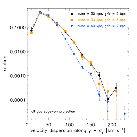
Figure 10: Pixelated velocity dispersion probability distribution (cf. Fig. 3 and the beginning of Section 3.1) of galaxies: resolution tests. Black circles and solid line: fiducial model with cube size = $30$ kpc and pixel size = $2$ kpc. Orange squares and triple dot-dashed line: cube size = $30$ kpc, pixel size = $3$ kpc. Blue inverted triangles and dot-dashed line: cube size = $60$ kpc, pixel size = $2$ kpc. Errors are Poissonian. We consider all gas in the edge-on xz projection $-$ $\sigma_{\rm y}$. Decreasing the resolution of the grid does not affect the $\sigma$-distribution, while changing the cube size from $30$ to $60$ kpc reduces the statistical relevance of the high-$\sigma$ tail.

To obtain the distribution described by the orange squares and triple dot-dashed line, we kept fixed the cube size to $30$ kpc and increased the pixel size to $3$ kpc. From Fig. 10, it is clear that the decrement in grid resolution does not affect much the new $\sigma$-distribution, which is essentially a smoothed version of the fiducial model.

On the other hand, changing the cube size from $30$ to $60$ kpc (while keeping the grid resolution fixed to $2$ kpc) has a large impact (blue inverted triangles and dot-dashed line). The new velocity dispersion distribution has a similar low-$\sigma$ part as the previous two, but declines more rapidly at $\sigma_{\rm y}>70$ km s^-1. This is due to the fact that the larger cubes include gas in the outskirts of galaxies, where the velocity dispersion is generally small. The additional pixels contribute mostly to the low-$\sigma$ part, while the increased total number of bins reduces the statistical relevance of the high-$\sigma$ tail.

Appendix B testing the methodology with idealized simulations of disc galaxies

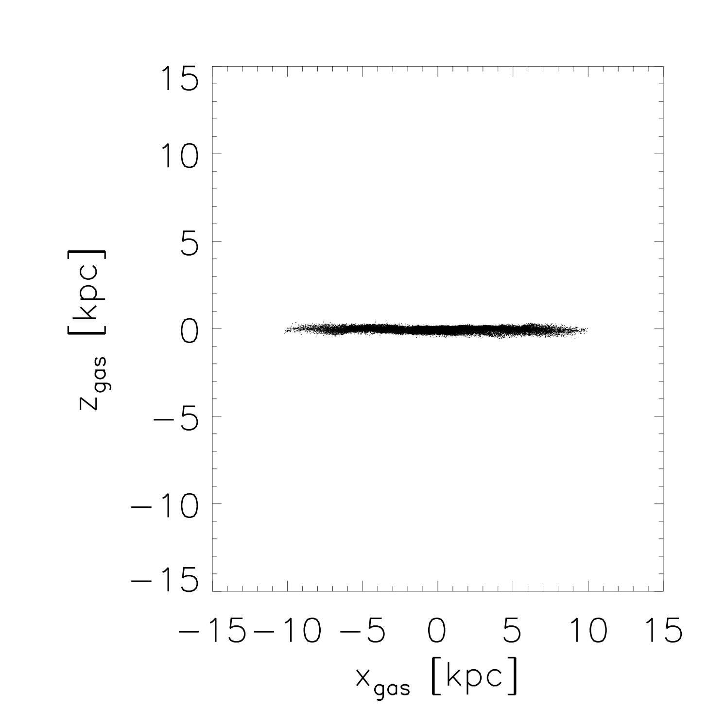
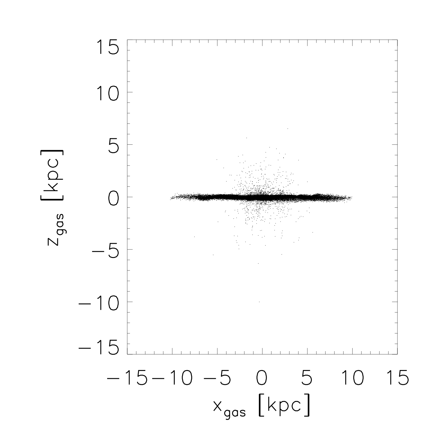
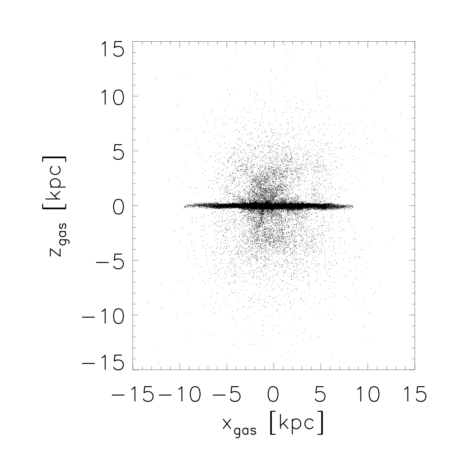
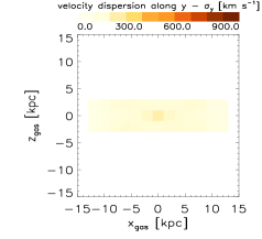
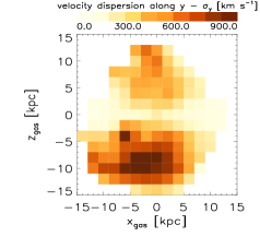
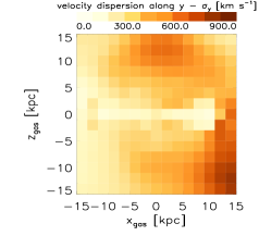
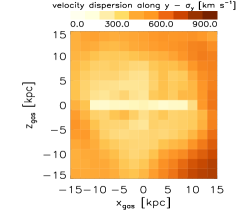
Figure 11: First row: positions in physical kpc of gas particles for our constrained disc galaxies. Second row: corresponding gas velocity dispersion maps. From left to right: the first column shows the no feedback run; second column $-$ weak feedback run; third column $-$ fiducial model; fourth column $-$ strong feedback run. In each panel, we consider all gas in the edge-on xz projection $-$ $\sigma_{\rm y}$.

Throughout this work, we have analysed galaxies extracted from one particular run of the EAGLE simulations: Recal-L025N0752. As discussed in Section 2.2, the L025N0752 configuration has the highest resolution of the set, and therefore comes in only two slightly different setups: Ref and Recal. Fully exploring the parameter space around the fiducial model would have been numerically too demanding, and was done instead using configurations with lower resolution (L050N0752 and L025N0376, see Crain et al., 2015). Consequently, we have not been able to study the impact of variations in the feedback strength, which are important for interpreting real data and also validating our previous results.

For this reason, we ran four simulations of an isolated disc galaxy. We used a different version of the GADGET-3 code that includes smoothed particle hydrodynamics with a higher order dissipation switch (SPHS) than classic SPH. The main advantage of SPHS is that it suppresses spurious numerical errors in the calculation of fluid quantities before they can propagate (Hobbs et al., 2013; Power et al., 2014). At temperatures T${}_{\rm gas}\geq 10^{4}$ K, the gas is assumed to be of primordial composition and cools radiatively following Katz et al. (1996). At T${}_{\rm floor}=100$ K $\leq$ T${}_{\rm gas}<10^{4}$ K, the gas cools following the prescription of Mashchenko et al. (2008) for gas of solar abundance. Gas is also prevented from cooling to the point at which the Jeans mass for gravitational collapse becomes unresolved. Gas above a fixed density threshold forms stars with a star formation efficiency of $10$% (Power & Robotham, 2016). The subgrid model for star formation is calibrated to follow the Kennicutt-Schmidt law (Kennicutt, 1998).

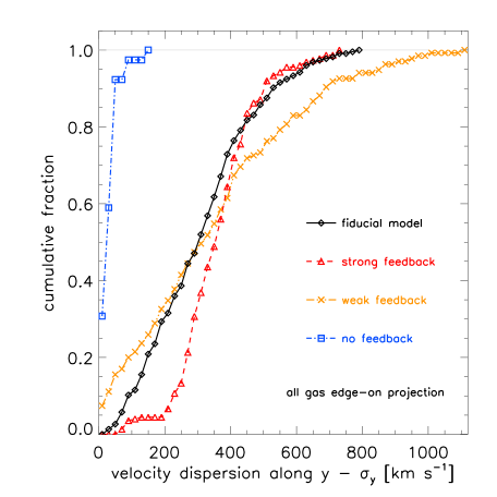
Figure 12: Cumulative fraction of the pixelated velocity dispersion probability distribution (cf. Fig. 3 and the beginning of Section 3.1) for our constrained disc galaxies. Black diamonds and solid line: fiducial model. Red triangles and dashed line: strong feedback. Orange crosses and triple dot-dashed line: weak feedback. Blue squares and dot-dashed line: no feedback. The thin grey horizontal line marks the saturation point of each distribution (cumulative fraction $=1$). We consider all gas in the edge-on xz projection $-$ $\sigma_{\rm y}$. As soon as feedback is introduced, the distributions shift to larger velocity dispersions.

The four constrained discs are identical in all but the strength of stellar feedback. The latter is quantified by the feedback factor $f_{\rm f}$, which simply (linearly) scales the amount of thermal energy deposited by supernovae into neighbouring gas particles. To calculate the energy released by SNe at any given time (where only SNe II are considered and $E_{\rm SN}=10^{51}$ erg), the code integrates over a Salpeter (1955) IMF in the range $8-100$ M_⊙ (to determine the number of SNe II) and adopts an approximate main-sequence time of $t_{\rm MS}\approx 11.8$ Myr. At $t_{\rm MS}$ after the formation of the star particle, the energy injection is implemented as a delta function in time (Hobbs et al., 2013). We varied the feedback factor from zero to strong feedback ($f_{\rm f}=1.50$), the fiducial model being the one with $f_{\rm f}=1.00$ (see Table 1). Each galaxy is composed of a (gas + stellar) disc of radius $10$ kpc and a stellar bulge embedded in a DM halo (with a NFW $-$ Navarro et al. 1996 $-$ concentration parameter $c=10$), sampled with $308,012$ total particles (of which N${}_{\rm DM}=100,000$). The mass and spatial resolutions are $1.6\times 10^{5}$ M_⊙ and $0.01$ kpc, respectively. All systems rotate (the DM halo spin parameter is $0.04$) and have the same total mass M${}_{\rm tot}=2.57\times 10^{12}$ M_⊙. Gas and stellar masses change according to $f_{\rm f}$ (as well as N_gas and N_⋆), with $\langle$M${}_{\star}\rangle=7.42\times 10^{10}$ M_⊙. We stress that these discs are not meant to faithfully reproduce physical and morphological properties of the EAGLE galaxies previously used. Our main goal here is testing the methodology.

Run	Feedback	$\max(\sigma_{\rm y})$
	factor ($f_{\rm f}$)	[km s-1]
strong feedback	1.50	738.74
fiducial model	1.00	786.67
weak feedback	0.75	1117.06
no feedback	0.00	157.30

Table 1: Run name, feedback factor $f_{\rm f}$ (that regulates the amount of thermal energy injected by SNe into nearby gas particles) and gas maximum velocity dispersion $\sigma_{\rm y}$ for the edge-on projection of our idealized disc galaxies.

In the first row of Fig. 11 we plot positions of gas particles for each single disc. From left to right, the following runs are shown: no feedback, weak feedback, fiducial model and strong feedback. We consider all gas in the edge-on xz projection. All systems are plotted at the same evolutionary stage of $t\sim 50$ Myr. As expected, the gas disc becomes more and more perturbed and the amount of outflowing material increases when moving from the no feedback to the strong feedback case. This trend is partially visible also in the second row of Fig. 11, where we show the corresponding gas velocity dispersion maps. It is interesting to note how the weak feedback run produces the largest velocity dispersions, $\max(\sigma_{\rm y})\approx 1120$ km s^-1 (see Table 1). This somewhat counterintuitive result is due to the fact that, compared to the fiducial and strong feedback simulations, only a few gas particles left the disc at the evolutionary stage considered and therefore the weak feedback $\sigma$-map is subjected to large statistical fluctuations.

In Fig. 12 the cumulative pixelated velocity dispersion probability distributions of the constrained discs are visible. We consider all gas in the edge-on xz projection $-$ $\sigma_{\rm y}$. The no feedback run quickly saturates to one at $\sigma_{\rm y}=150$ km s^-1. In this case, only the disc component is present (according to the leftmost panel in the second row of Fig. 11). This $\sigma$-distribution is statistically different from the other three. As soon as feedback is introduced, the distributions shift to progressively larger velocity dispersions following the increase in feedback strength. This is particularly visible up to $\sigma_{\rm y}\sim 400$ km s^-1, where there is a crossover between the weak feedback (orange crosses and triple dot-dashed line) and the strong feedback (red triangles and dashed line) runs for the reason explained in the previous paragraph.

These trends fully support the low-$\sigma$ $\Leftrightarrow$ disc + high-$\sigma$ $\Leftrightarrow$ outflows correlations emerging from the analysis of EAGLE galaxies presented in the paper. We refrained from calculating the $\xi$ and $\eta_{50}$ parameters for the constrained discs because the results would be completely dominated by statistical noise$/$fluctuations.

References

- Allen et al. (2015) Allen J. T., et al., 2015, MNRAS, 446, 1567
- Altay & Theuns (2013) Altay G., Theuns T., 2013, MNRAS, 434, 748
- Anglés-Alcázar et al. (2017) Anglés-Alcázar D., Faucher-Giguère C.-A., Kereš D., Hopkins P. F., Quataert E., Murray N., 2017, MNRAS, 470, 4698
- Bahé et al. (2016) Bahé Y. M., et al., 2016, MNRAS, 456, 1115
- Barai et al. (2013) Barai P., et al., 2013, MNRAS, 430, 3213
- Barai et al. (2015) Barai P., Monaco P., Murante G., Ragagnin A., Viel M., 2015, MNRAS, 447, 266
- Bershady et al. (2010) Bershady M. A., Verheijen M. A. W., Swaters R. A., Andersen D. R., Westfall K. B., Martinsson T., 2010, ApJ, 716, 198
- Bland-Hawthorn (2015) Bland-Hawthorn J., 2015, in Ziegler B. L., Combes F., Dannerbauer H., Verdugo M., eds, IAU Symposium Vol. 309, Galaxies in 3D across the Universe. pp 21–28 (arXiv:1410.3838), doi:10.1017/S1743921314009247
- Bland-Hawthorn & Cohen (2003) Bland-Hawthorn J., Cohen M., 2003, ApJ, 582, 246
- Bland-Hawthorn et al. (2007) Bland-Hawthorn J., Veilleux S., Cecil G., 2007, Ap&SS, 311, 87
- Bland-Hawthorn et al. (2011) Bland-Hawthorn J., et al., 2011, Optics Express, 19, 2649
- Bower et al. (2017) Bower R. G., Schaye J., Frenk C. S., Theuns T., Schaller M., Crain R. A., McAlpine S., 2017, MNRAS, 465, 32
- Brüggen & Scannapieco (2016) Brüggen M., Scannapieco E., 2016, ApJ, 822, 31
- Bryant et al. (2014) Bryant J. J., Bland-Hawthorn J., Fogarty L. M. R., Lawrence J. S., Croom S. M., 2014, MNRAS, 438, 869
- Bryant et al. (2015) Bryant J. J., et al., 2015, MNRAS, 447, 2857
- Bryant et al. (2016) Bryant J. J., et al., 2016, in Ground-based and Airborne Instrumentation for Astronomy VI. p. 99081F (arXiv:1608.03921), doi:10.1117/12.2230740
- Bundy et al. (2015) Bundy K., et al., 2015, ApJ, 798, 7
- Bustard et al. (2016) Bustard C., Zweibel E. G., D’Onghia E., 2016, ApJ, 819, 29
- Cappellari (2016) Cappellari M., 2016, ARA&A, 54, 597
- Cappellari et al. (2011) Cappellari M., et al., 2011, MNRAS, 413, 813
- Ceverino et al. (2016) Ceverino D., Arribas S., Colina L., Rodríguez Del Pino B., Dekel A., Primack J., 2016, MNRAS, 460, 2731
- Chabrier (2003) Chabrier G., 2003, PASP, 115, 763
- Chisholm et al. (2016a) Chisholm J., Tremonti C. A., Leitherer C., Chen Y., Wofford A., 2016a, MNRAS, 457, 3133
- Chisholm et al. (2016b) Chisholm J., Tremonti Christy A., Leitherer C., Chen Y., 2016b, MNRAS, 463, 541
- Christensen et al. (2016) Christensen C. R., Davé R., Governato F., Pontzen A., Brooks A., Munshi F., Quinn T., Wadsley J., 2016, ApJ, 824, 57
- Cicone et al. (2016) Cicone C., Maiolino R., Marconi A., 2016, A&A, 588, A41
- Cooper et al. (2008) Cooper J. L., Bicknell G. V., Sutherland R. S., Bland-Hawthorn J., 2008, ApJ, 674, 157
- Cooper et al. (2009) Cooper J. L., Bicknell G. V., Sutherland R. S., Bland-Hawthorn J., 2009, ApJ, 703, 330
- Crain et al. (2015) Crain R. A., et al., 2015, MNRAS, 450, 1937
- Croom et al. (2012) Croom S. M., et al., 2012, MNRAS, 421, 872
- Dale (2015) Dale J. E., 2015, New Astron. Rev., 68, 1
- Dalla Vecchia & Schaye (2012) Dalla Vecchia C., Schaye J., 2012, MNRAS, 426, 140
- Dolag et al. (2009) Dolag K., Borgani S., Murante G., Springel V., 2009, MNRAS, 399, 497
- Fogarty et al. (2012) Fogarty L. M. R., et al., 2012, ApJ, 761, 169
- Furlong et al. (2017) Furlong M., et al., 2017, MNRAS, 465, 722
- Girichidis et al. (2016) Girichidis P., et al., 2016, MNRAS, 456, 3432
- Green et al. (2017) Green A. W., et al., 2017, preprint, (arXiv:1707.08402)
- Guidi et al. (2016a) Guidi G., Casado J., Ascasibar Y., Galbany L., Sánchez-Blázquez P., Sánchez S. F., Fabián Rosales-Ortega F., Scannapieco C., 2016a, preprint, (arXiv:1610.07620)
- Guidi et al. (2016b) Guidi G., Scannapieco C., Walcher J., Gallazzi A., 2016b, MNRAS, 462, 2046
- Hayward & Hopkins (2017) Hayward C. C., Hopkins P. F., 2017, MNRAS, 465, 1682
- Heckman (2002) Heckman T. M., 2002, in Mulchaey J. S., Stocke J. T., eds, Astronomical Society of the Pacific Conference Series Vol. 254, Extragalactic Gas at Low Redshift. p. 292 (arXiv:astro-ph/0107438)
- Heckman et al. (2015) Heckman T. M., Alexandroff R. M., Borthakur S., Overzier R., Leitherer C., 2015, ApJ, 809, 147
- Ho et al. (2014) Ho I.-T., et al., 2014, MNRAS, 444, 3894
- Ho et al. (2016a) Ho I.-T., et al., 2016a, Ap&SS, 361, 280
- Ho et al. (2016b) Ho I.-T., et al., 2016b, MNRAS, 457, 1257
- Hobbs et al. (2013) Hobbs A., Read J., Power C., Cole D., 2013, MNRAS, 434, 1849
- Kacprzak et al. (2015) Kacprzak G. G., Muzahid S., Churchill C. W., Nielsen N. M., Charlton J. C., 2015, ApJ, 815, 22
- Katz et al. (1996) Katz N., Weinberg D. H., Hernquist L., 1996, ApJS, 105, 19
- Keller et al. (2015) Keller B. W., Wadsley J., Couchman H. M. P., 2015, MNRAS, 453, 3499
- Kennicutt (1998) Kennicutt Jr. R. C., 1998, ARA&A, 36, 189
- Kim et al. (2017) Kim C.-G., Ostriker E. C., Raileanu R., 2017, ApJ, 834, 25
- Lawrence et al. (2012) Lawrence J., et al., 2012, in Ground-based and Airborne Instrumentation for Astronomy IV. p. 844653, doi:10.1117/12.925260
- Leitherer et al. (2013) Leitherer C., Chandar R., Tremonti C. A., Wofford A., Schaerer D., 2013, ApJ, 772, 120
- Leslie et al. (2017) Leslie S. K., et al., 2017, preprint, (arXiv:1707.03879)
- Li et al. (2015) Li M., Ostriker J. P., Cen R., Bryan G. L., Naab T., 2015, ApJ, 814, 4
- Li et al. (2017) Li M., Bryan G. L., Ostriker J. P., 2017, ApJ, 841, 101
- Martin et al. (2012) Martin C. L., Shapley A. E., Coil A. L., Kornei K. A., Bundy K., Weiner B. J., Noeske K. G., Schiminovich D., 2012, ApJ, 760, 127
- Martizzi et al. (2016) Martizzi D., Fielding D., Faucher-Giguère C.-A., Quataert E., 2016, MNRAS, 459, 2311
- Mashchenko et al. (2008) Mashchenko S., Wadsley J., Couchman H. M. P., 2008, Science, 319, 174
- McKee & Ostriker (1977) McKee C. F., Ostriker J. P., 1977, ApJ, 218, 148
- Meiksin (2016) Meiksin A., 2016, MNRAS, 461, 2762
- Muratov et al. (2015) Muratov A. L., Kereš D., Faucher-Giguère C.-A., Hopkins P. F., Quataert E., Murray N., 2015, MNRAS, 454, 2691
- Murray et al. (2011) Murray N., Ménard B., Thompson T. A., 2011, ApJ, 735, 66
- Naab et al. (2014) Naab T., et al., 2014, MNRAS, 444, 3357
- Navarro et al. (1996) Navarro J. F., Frenk C. S., White S. D. M., 1996, ApJ, 462, 563
- Nelson et al. (2015) Nelson D., Genel S., Vogelsberger M., Springel V., Sijacki D., Torrey P., Hernquist L., 2015, MNRAS, 448, 59
- Nestor et al. (2011) Nestor D. B., Johnson B. D., Wild V., Ménard B., Turnshek D. A., Rao S., Pettini M., 2011, MNRAS, 412, 1559
- Oppenheimer et al. (2010) Oppenheimer B. D., Davé R., Kereš D., Fardal M., Katz N., Kollmeier J. A., Weinberg D. H., 2010, MNRAS, 406, 2325
- Pereira-Santaella et al. (2016) Pereira-Santaella M., et al., 2016, A&A, 594, A81
- Planck Collaboration et al. (2014) Planck Collaboration et al., 2014, A&A, 571, A1
- Power & Robotham (2016) Power C., Robotham A. S. G., 2016, ApJ, 825, 31
- Power et al. (2014) Power C., Read J. I., Hobbs A., 2014, MNRAS, 440, 3243
- Renzini & Peng (2015) Renzini A., Peng Y.-j., 2015, ApJ, 801, L29
- Rosdahl et al. (2015) Rosdahl J., Schaye J., Teyssier R., Agertz O., 2015, MNRAS, 451, 34
- Rubin et al. (2014) Rubin K. H. R., Prochaska J. X., Koo D. C., Phillips A. C., Martin C. L., Winstrom L. O., 2014, ApJ, 794, 156
- Ruszkowski et al. (2017) Ruszkowski M., Yang H.-Y. K., Zweibel E., 2017, ApJ, 834, 208
- Salem & Bryan (2014) Salem M., Bryan G. L., 2014, MNRAS, 437, 3312
- Salpeter (1955) Salpeter E. E., 1955, ApJ, 121, 161
- Sánchez et al. (2012) Sánchez S. F., et al., 2012, A&A, 538, A8
- Sarzi et al. (2016) Sarzi M., Kaviraj S., Nedelchev B., Tiffany J., Shabala S. S., Deller A. T., Middelberg E., 2016, MNRAS, 456, L25
- Scannapieco & Brüggen (2015) Scannapieco E., Brüggen M., 2015, ApJ, 805, 158
- Schaller et al. (2015) Schaller M., Dalla Vecchia C., Schaye J., Bower R. G., Theuns T., Crain R. A., Furlong M., McCarthy I. G., 2015, MNRAS, 454, 2277
- Schaye & Dalla Vecchia (2008) Schaye J., Dalla Vecchia C., 2008, MNRAS, 383, 1210
- Schaye et al. (2015) Schaye J., et al., 2015, MNRAS, 446, 521
- Schneider & Robertson (2017) Schneider E. E., Robertson B. E., 2017, ApJ, 834, 144
- Shapley (2011) Shapley A. E., 2011, ARA&A, 49, 525
- Sharma et al. (2017) Sharma M., Theuns T., Frenk C., Bower R. G., Crain R. A., Schaller M., Schaye J., 2017, MNRAS, 468, 2176
- Sharp & Bland-Hawthorn (2010) Sharp R. G., Bland-Hawthorn J., 2010, ApJ, 711, 818
- Sharp et al. (2006) Sharp R., et al., 2006, in Society of Photo-Optical Instrumentation Engineers (SPIE) Conference Series. p. 62690G (arXiv:astro-ph/0606137), doi:10.1117/12.671022
- Sharp et al. (2015) Sharp R., et al., 2015, MNRAS, 446, 1551
- Somerville & Davé (2015) Somerville R. S., Davé R., 2015, ARA&A, 53, 51
- Springel (2005) Springel V., 2005, MNRAS, 364, 1105
- Springel & Hernquist (2003) Springel V., Hernquist L., 2003, MNRAS, 339, 289
- Springel et al. (2001) Springel V., White S. D. M., Tormen G., Kauffmann G., 2001, MNRAS, 328, 726
- Steidel et al. (2010) Steidel C. C., Erb D. K., Shapley A. E., Pettini M., Reddy N., Bogosavljević M., Rudie G. C., Rakic O., 2010, ApJ, 717, 289
- Tanner et al. (2016) Tanner R., Cecil G., Heitsch F., 2016, ApJ, 821, 7
- Tanner et al. (2017) Tanner R., Cecil G., Heitsch F., 2017, ApJ, 843, 137
- Tescari et al. (2014) Tescari E., Katsianis A., Wyithe J. S. B., Dolag K., Tornatore L., Barai P., Viel M., Borgani S., 2014, MNRAS, 438, 3490
- Thompson et al. (2016) Thompson T. A., Quataert E., Zhang D., Weinberg D. H., 2016, MNRAS, 455, 1830
- Trayford et al. (2015) Trayford J. W., et al., 2015, MNRAS, 452, 2879
- Turner et al. (2016) Turner M. L., Schaye J., Crain R. A., Theuns T., Wendt M., 2016, MNRAS, 462, 2440
- Veilleux et al. (2005) Veilleux S., Cecil G., Bland-Hawthorn J., 2005, ARA&A, 43, 769
- Wiener et al. (2017) Wiener J., Pfrommer C., Oh S. P., 2017, MNRAS, 467, 906
- Wiersma et al. (2009a) Wiersma R. P. C., Schaye J., Smith B. D., 2009a, MNRAS, 393, 99
- Wiersma et al. (2009b) Wiersma R. P. C., Schaye J., Theuns T., Dalla Vecchia C., Tornatore L., 2009b, MNRAS, 399, 574
- Zhang & Davis (2017) Zhang D., Davis S. W., 2017, ApJ, 839, 54
- Zhang et al. (2017) Zhang D., Thompson T. A., Quataert E., Murray N., 2017, MNRAS, 468, 4801
- Zhu et al. (2015) Zhu G. B., et al., 2015, ApJ, 815, 48